Embed Size (px)
DESCRIPTION
aspenONE
Citation preview
Aspen Polymers Plus
Examples & Applications

Version Number: 2006 October 2006
Copyright (c) 2006 by Aspen Technology, Inc. All rights reserved.
Aspen Polymers Plus, aspenONE, the aspen leaf logo and Plantelligence and Enterprise Optimization are trademarks or registered trademarks of Aspen Technology, Inc., Cambridge, MA.
All other brand and product names are trademarks or registered trademarks of their respective companies.
This document is intended as a guide to using AspenTech's software. This documentation contains AspenTech proprietary and confidential information and may not be disclosed, used, or copied without the prior consent of AspenTech or as set forth in the applicable license agreement. Users are solely responsible for the proper use of the software and the application of the results obtained.
Although AspenTech has tested the software and reviewed the documentation, the sole warranty for the software may be found in the applicable license agreement between AspenTech and the user. ASPENTECH MAKES NO WARRANTY OR REPRESENTATION, EITHER EXPRESSED OR IMPLIED, WITH RESPECT TO THIS DOCUMENTATION, ITS QUALITY, PERFORMANCE, MERCHANTABILITY, OR FITNESS FOR A PARTICULAR PURPOSE.
Aspen Technology, Inc. Ten Canal Park Cambridge, MA 02141-2201 USA Phone: (1) (617) 949-1000 Toll Free: (1) (888) 996-7001 Fax: (1) (617) 949-1030 URL: http://www.aspentech.com
Contents iii
Contents
Introducing Aspen Polymers Plus ...........................................................................1 About This Manual.......................................................................................... 1 Related Documentation................................................................................... 3 Technical Support .......................................................................................... 3
A1 Creating a Simulation Model..............................................................................5 Creating a New Run........................................................................................ 5 Creating the Process Flowsheet ........................................................................ 6
Placing Blocks and Streams ................................................................... 6 Renaming Blocks and Streams ............................................................... 7
Specifying Setup and Global Options................................................................. 7 Entering a Simulation Title..................................................................... 8 Defining Unit-Sets ................................................................................ 8 Entering a Simulation Description ........................................................... 8 Defining Report Options ........................................................................ 9 Specifying Other Simulation Options ....................................................... 9
Specifying Components................................................................................... 9 Characterizing Polymers.................................................................................10 Specifying Physical Properties .........................................................................11 Specifying Feed Streams ................................................................................12 Specifying Kinetics ........................................................................................13
Modifying Reactions.............................................................................13 Specifying Gel Effect............................................................................15
Defining the Unit Operation Block ....................................................................16 Entering Block Specifications.................................................................16 Improving Convergence .......................................................................17 Overriding Global Values ......................................................................17 Entering Mixer Specifications ................................................................17
Running the Simulation..................................................................................18 Examining Simulation Results .........................................................................18
Input Summary ..................................................................................19 Plotting Distributions .....................................................................................22 Creating Live Distribution Plots........................................................................23
Viewing Plots for Multiple Simulations.....................................................24 Pasting and Linking Between Aspen Polymers Plus and Excel ...............................26 Saving the Run and Exiting.............................................................................27
A2 Predicting Physical Properties.........................................................................28 Defining the Simulation..................................................................................29
Creating a New Run.............................................................................29 Specifying Setup and Global Options ......................................................30 Specifying and Characterizing Components .............................................30
iv Contents
Specifying Physical Properties ...............................................................31 Defining Molecular Structure .................................................................32 Specifying Mass Fraction Crystallinity .....................................................33 Creating Property Sets .........................................................................33 Creating Property Tables ......................................................................34
Running the Simulation and Examining the Results ............................................35 Input Summary ..................................................................................37
References ...................................................................................................38
A3 Regressing Property Parameters.....................................................................39 Defining the Simulation..................................................................................40
Creating a New Run.............................................................................40 Specifying Setup and Global Options ......................................................40 Specifying and Characterizing Components .............................................41 Specifying Physical Property Method ......................................................42 Entering Experimental Data ..................................................................42 Specifying a Regression Case................................................................45 Specifying Physical Property Parameters.................................................46
Running the Simulation and Examining the Results ............................................47 Input Summary ..................................................................................48
References ...................................................................................................50
A4 Fitting Kinetic Parameters...............................................................................51 Defining the Simulation..................................................................................52
Creating a New Run.............................................................................52 Creating the Process Flowsheet .............................................................52 Specifying Setup and Global Options ......................................................54 Specifying and Characterizing Components .............................................55 Specifying Physical Properties ...............................................................56 Specifying Polymerization Kinetics .........................................................57 Supplying Process Information ..............................................................59 Specifying Data Regression...................................................................61
Running the Simulation and Examining the Results ............................................65 Input Summary ..................................................................................66
A5 Fractionating Oligomers..................................................................................69 Defining the Simulation..................................................................................69
Creating a New Run.............................................................................70 Creating the Process Flowsheet .............................................................70 Specifying Setup and Global Options ......................................................71 Specifying and Characterizing Components .............................................72 Specifying Physical Properties ...............................................................73 Supplying Process Information ..............................................................76
Running the Simulation and Examining the Results ............................................77 Input Summary ..................................................................................79
References ...................................................................................................81
A6 Calculating End-Use Properties .......................................................................82 Defining the Simulation..................................................................................82
Creating a New Run.............................................................................83 Creating the Process Flowsheet .............................................................83
Contents v
Specifying Setup and Global Options ......................................................84 Specifying and Characterizing Components .............................................84 Specifying Physical Properties ...............................................................85 Supplying Process Information ..............................................................86 Creating a Sensitivity Table ..................................................................87
Running the Simulation and Examining the Results ............................................89 Input Summary ..................................................................................89
References ...................................................................................................91
Section B - User Models.........................................................................................92 Installing Polymer User Model Library...............................................................92
B1 Polymer Fractionation Algorithm.....................................................................94 Installing the Polymer Fractionation Examples ...................................................95
Creating a Working Directory ................................................................95 Developing a Proprietary Model .......................................................................95
Opening the Model ..............................................................................95 Specifying Pseudo-Componenets ...........................................................95 Running the Example...........................................................................96
Example Polymer Fractionation Model - PolFrac1................................................96 Input Summary ..................................................................................97 Stream Report ..................................................................................100
Example Polymer Fractionation Model - PolFrac2..............................................103 Input Summary ................................................................................106 Stream Report ..................................................................................108
References .................................................................................................109
B2 Aspen Polymers Plus-Predici Interface .........................................................110 Developing a Proprietary Model .....................................................................110
Opening the Model ............................................................................110 Mapping the Components ...................................................................111 Specifying Stream Flash .....................................................................113 Running the Example.........................................................................114
Example Predici Four CSTR Model..................................................................114 Results ............................................................................................115 Input Summary ................................................................................116 Stream Report ..................................................................................118
C1 Polystyrene Bulk Polymerization by Thermal Initiation.................................121 About This Process ......................................................................................121 Process Definition........................................................................................121
Process Conditions ............................................................................122 Physical Property Models and Data.......................................................123 Reactors / Kinetics ............................................................................123 Process Studies.................................................................................124
Selected Simulation Results..........................................................................128 Simulation Stream Summary ..............................................................130
References .................................................................................................132
vi Contents
C2 Polystyrene with Styrene Monomer Distillation.............................................133 About This Process ......................................................................................133 Process Definition........................................................................................133
Process Conditions ............................................................................134 Polymers and Segments .....................................................................135 Physical Property Models and Data.......................................................135 Reactors / Kinetics ............................................................................136 Inhibitor ..........................................................................................136 Process Studies.................................................................................136
Selected Simulation Results..........................................................................141 Simulation Stream Summary ..............................................................143
References .................................................................................................146
C3 Expanded Polystyrene Suspension Polymerization........................................147 About This Process ......................................................................................147 Process Definition........................................................................................148
Process Conditions ............................................................................149 Physical Property Models and Data.......................................................150 Reactors / Kinetics ............................................................................150 Process Studies.................................................................................151
Selected Simulation Results..........................................................................154 References .................................................................................................156
C4 Styrene Ethyl Acrylate Free-Radical Copolymerization Process .....................157 About This Process ......................................................................................157 Process Definition........................................................................................157
Process Conditions ............................................................................158 Reactors / Kinetics ............................................................................158 Parameter Regression ........................................................................160 Process Studies.................................................................................163
Selected Simulation Results..........................................................................167 References .................................................................................................171
C5 Styrene Butadiene Emulsion Copolymerization Process ................................172 About This Process ......................................................................................172 Process Definition........................................................................................173
Process Conditions ............................................................................173 Physical Property Models and Data.......................................................175 Reactors / Kinetics ............................................................................175 Process Studies.................................................................................176
Selected Simulation Results..........................................................................180 References .................................................................................................183
C6 Styrene Butadiene Ionic Polymerization Processes .......................................184 About This Process ......................................................................................184 Process Definition........................................................................................185
Process Conditions ............................................................................186 Kinetics ...........................................................................................186 Process Studies.................................................................................187
Selected Simulation Results..........................................................................189
Contents vii
C7 High-Density Polyethylene High Temperature Solution Process ....................192 About This Process ......................................................................................192 Process Definition........................................................................................193
Process Conditions ............................................................................193 Reactors / Kinetics ............................................................................194 Process Studies.................................................................................194
Selected Simulation Results..........................................................................200 Simulation Stream Summary ..............................................................205
References .................................................................................................210
C8 Low-Density Polyethylene High Pressure Process .........................................211 About This Process ......................................................................................211 Process Definition........................................................................................211
Process Conditions ............................................................................213 Physical Property Models and Data.......................................................214 Process Studies.................................................................................215
Selected Simulation Results..........................................................................219 Simulation Stream Summary ..............................................................222
References .................................................................................................228
C9 Nylon 6 Caprolactam Polymerization Process................................................230 About This Process ......................................................................................230 Process Definition........................................................................................231
Process Conditions ............................................................................232 Physical Property Models and Data.......................................................233 Reaction Kinetics...............................................................................233 Process Studies.................................................................................239
Selected Simulation Results..........................................................................244 Simulation Stream Summary ..............................................................245
References .................................................................................................248
C10 Methyl Methacrylate Polymerization in Ethyl Acetate ..................................249 About This Process ......................................................................................249 Process Definition........................................................................................249
Process Conditions ............................................................................250 Reactors / Kinetics ............................................................................251 Process Studies.................................................................................251
Selected Simulation Results..........................................................................253 References .................................................................................................258
C11 Polypropylene Gas Phase Polymerization Processes ...................................259 About This Process ......................................................................................259 Process Definition........................................................................................260
Process Conditions ............................................................................261 Physical Property Models and Data.......................................................263 Reactors / Kinetics ............................................................................263 Process Studies.................................................................................264
Selected Simulation Results..........................................................................269 Simulation Stream Summary ..............................................................269
References .................................................................................................277
viii Contents
Index ..................................................................................................................278
Introducing Aspen Polymers Plus 1
Introducing Aspen Polymers Plus
Aspen Polymers Plus is a general-purpose process modeling system for the simulation of polymer manufacturing processes. The modeling system includes modules for the estimation of thermophysical properties, and for performing polymerization kinetic calculations and associated mass and energy balances.
Also included in Aspen Polymers Plus are modules for:
• Characterizing polymer molecular structure
• Calculating rheological and mechanical properties
• Tracking these properties throughout a flowsheet
There are also many additional features that permit the simulation of the entire manufacturing processes. This casebook is a compilation of simulation examples, user models, and industrial application examples.
Note: Some of the simulations described in this book require Fortran files. These are found in the same location as the simulation files (\xmp or \app sub-directory of the GUI installation directory). You must compile the accompanying Fortran before running the files.
About This Manual The Aspen Polymers Plus Examples & Applications Casebook is divided into three sections:
• Section A – Simulation Examples provides step-by-step instructions for using Aspen Polymers Plus® to build and use a polymer process simulation model. Topics include:
o Creating a simulation model
o Predicting physical properties
o Regressing property parameters
o Fitting kinetic parameters
o Fractionating oligomers
o Calculating end-use properties
2 Introducing Aspen Polymers Plus
• Section B – User Models provides step-by–step instructions for using and customizing currently available User2 models. Topics include: o Four-phase equilibrium TP-Flash
o Polymer fractionation algorithm
o User-specified molecular weight distribution for feed streams
o Aspen Polymers Plus – Predici interface
• Section C – Application Examples presents common industrial processes and describes how to simulate the reactor section of specific polymer production processes. A few of the application examples describe a complete plant flowsheet, and others focus on physical property representation. Topics include: o Polystyrene bulk polymerization by thermal initiation
o Polystyrene with styrene monomer distillation
o Expanded polystyrene suspension polymerization
o Styrene ethyl acrylate free-radical copolymerization process
o Styrene butadiene emulsion copolymerization process
o Styrene butadiene ionic polymerization processes
o High-density polyethylene high temperature solution process
o Low-density polyethylene high pressure process
o Nylon 6 caprolactam polymerization process
o Methyl methacrylate polymerization in ethyl acetate
o Polypropylene gas phase polymerization processes
Note: Dynamic process applications are available in the Aspen Dynamics™ Examples documentation set.
Introducing Aspen Polymers Plus 3
Related Documentation
In addition to this document, a number of other documents are provided to help users learn and use Aspen Polymers Plus applications. The documentation set consists of the following:
Installation Guides
Aspen Engineering Suite Installation Guide
Aspen Polymers Plus Guides
Aspen Polymers Plus User Guide, Volume 1
Aspen Polymers Plus User Guide, Volume 2 (Physical Property Methods & Models)
Aspen Plus Guides
Aspen Plus User Guide
Aspen Plus Getting Started Guides
Aspen Dynamics Guides
Aspen Dynamics Examples
Aspen Dynamics User Guide
Aspen Dynamics Reference Guide
Technical Support AspenTech customers with a valid license and software maintenance agreement can register to access the online AspenTech Support Center at:
http://support.aspentech.com
This Web support site allows you to:
• Access current product documentation
• Search for tech tips, solutions and frequently asked questions (FAQs)
• Search for and download application examples
• Search for and download service packs and product updates
• Submit and track technical issues
• Send suggestions
• Report product defects
• Review lists of known deficiencies and defects

4 Introducing Aspen Polymers Plus
Registered users can also subscribe to our Technical Support e-Bulletins. These e-Bulletins are used to alert users to important technical support information such as:
• Technical advisories
• Product updates and releases
Customer support is also available by phone, fax, and email. The most up-to-date contact information is available at the AspenTech Support Center at http://support.aspentech.com.
A1 Creating a Simulation Model 5
A1 Creating a Simulation Model
This example describes how to construct a polymer simulation model. It provides an overview of Aspen Polymers Plus features.
The steps covered include:
• Creating a New Run
• Creating the Process Flowsheet
• Specifying Setup and Global Options
• Specifying Components
• Characterizing Polymers
• Specifying Physical Properties
• Specifying Feed Streams
• Specifying Kinetics
• Defining the Unit Operation Block
• Running the Simulation
• Examining Simulation Results
• Plotting Distributions
• Creating Live Distribution Plots
• Pasting and Linking Between Aspen Polymers Plus and Excel
• Saving the Run and Exiting
The process in this example uses two CSTR reactors and a mixer. The free-radical kinetics occur in the reactors.
Creating a New Run To construct the simulation model you need to start Aspen Polymers Plus.
To start Aspen Polymers Plus:
1 Start Aspen Plus from the Start Menu or by double clicking the Aspen Plus icon on your desktop.
The Aspen Plus Startup dialog box appears.
6 A1 Creating a Simulation Model
2 On the Aspen Plus Startup dialog box, click the Template option. Click OK.
The New dialog box appears. You use this dialog box to specify the simulation template and Run Type for the new run. Aspen Plus uses the Simulation Template you choose to automatically set various defaults appropriate to your application.
3 For this example, click Polymers with Metric Units for your template. The default Run type, Flowsheet, is appropriate. Click OK.
The Aspen Plus main window is now active.
Creating the Process Flowsheet In a flowsheet you can:
• Place (or delete) blocks
• Place (or delete) streams
• Rename blocks and streams
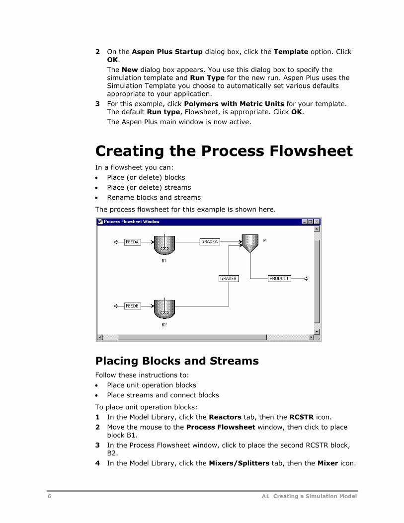
The process flowsheet for this example is shown here.
Placing Blocks and Streams Follow these instructions to:
• Place unit operation blocks
• Place streams and connect blocks
To place unit operation blocks:
1 In the Model Library, click the Reactors tab, then the RCSTR icon.
2 Move the mouse to the Process Flowsheet window, then click to place block B1.
3 In the Process Flowsheet window, click to place the second RCSTR block, B2.
4 In the Model Library, click the Mixers/Splitters tab, then the Mixer icon.
A1 Creating a Simulation Model 7
If you want to select different Mixer model icons, click the down-arrow on the icon.
To place streams:
1 Click the Material STREAMS icon on the left corner of the Model Library and move the mouse to the Process Flowsheet window.
Red and blue arrows appear on the unit operation blocks. These arrows indicate the location of the required (red) and optional (blue) stream connection ports.
2 Place the “+” cursor on the red feed arrow of B1 and click to make the connection. Move the mouse away from the block and click again to place stream 1 (FEEDA).
3 Place the “+” cursor on the red product arrow of B1 and click to make the connection. Move the mouse to the red feed arrow of B3 (M) and click again to connect the two blocks. Refer to the process flowsheet for the location of these streams.
4 Repeat these steps to create a feed stream for B2, connect B2 and B3 (M), and create a product stream for B3 (M).
5 After placing all streams, turn off the insert mode by clicking the Select
Mode button in the upper left corner of the Model Library.
Renaming Blocks and Streams To rename blocks and streams:
1 Click the block to be renamed, such as B3, and click the right mouse button to display the menu.
2 Click Rename Block.
3 Enter the Block ID as “M” and click OK.
4 Click the stream to be renamed, such as 1, and click the right mouse button to display the menu.
5 Click Rename Stream.
6 Enter the Stream ID as “FEEDA” and click OK.
7 Repeat these steps to rename the other streams.
You are now ready to enter input data for your simulation.
Specifying Setup and Global Options To enter process and model specifications into Aspen Polymers Plus, you can
use the Next button or the Data Browser Menu Tree. In this example, you enter data using the Menu Tree.
Use the Setup folder to:
• Enter a simulation title
• Define unit-sets
8 A1 Creating a Simulation Model
• Review and specify global options set by the simulation template you selected
Entering a Simulation Title To enter a title:
1 From the Data menu, click Setup.
The Setup Specifications - Data Browser appears.
2 On the Global sheet, type the title of your simulation run as: Creating an Aspen Polymers Plus Simulation Model
Defining Unit-Sets This example requires a user defined unit-set for input data and output results.
To define a unit-set:
1 From the Setup folder in the Menu Tree, double-click the Units-Sets sub-folder.
2 Click New to create a new set.
3 Enter an ID (for example, SET1) and click OK.
A dialog box appears requesting approval to make SET1 the global unit set, click Yes.
4 Confirm that SI is entered in the Copy from field. If it is not selected, select SI from the pulldown list. This means the simulation will use SI units as the basis for your new unit set.
5 Set the following options: o Mass Flow = kg/hr
o Mole Flow = kmol/hr
o Temperature = C
o Pressure = atm
Entering a Simulation Description A Description sheet is available to enter a more detailed description of the simulation.
To enter the description for this example:
1 From the Setup folder in the Menu Tree, click the Specifications form.
2 Click the Description tab.
You can either retain or delete the default information displayed, but type the following description: This example describes how to put together a polymer simulation model.
A1 Creating a Simulation Model 9
Defining Report Options Since you chose the Polymers with Metric Units simulation template when you started this example, Aspen Plus has set defaults for calculating and reporting stream properties:
• No mole flow
• Mass flow
To enter a user defined stream report format:
1 From the Setup folder in the Menu Tree, click the Report Options form.
2 Click the Stream tab.
3 In addition to the default options, click Mole for the Flow basis frame and Mass for the Fraction basis frame.
Specifying Other Simulation Options To enter other simulation options for this example:
1 From the Setup folder in the Menu Tree, click the Simulation Options form.
2 Click the Limits tab.
3 Enter 1000 in the Simulation time limit in CPU seconds field.
4 Click the System tab, and click the Print Fortran tracebacks when a Fortran error occurs option.
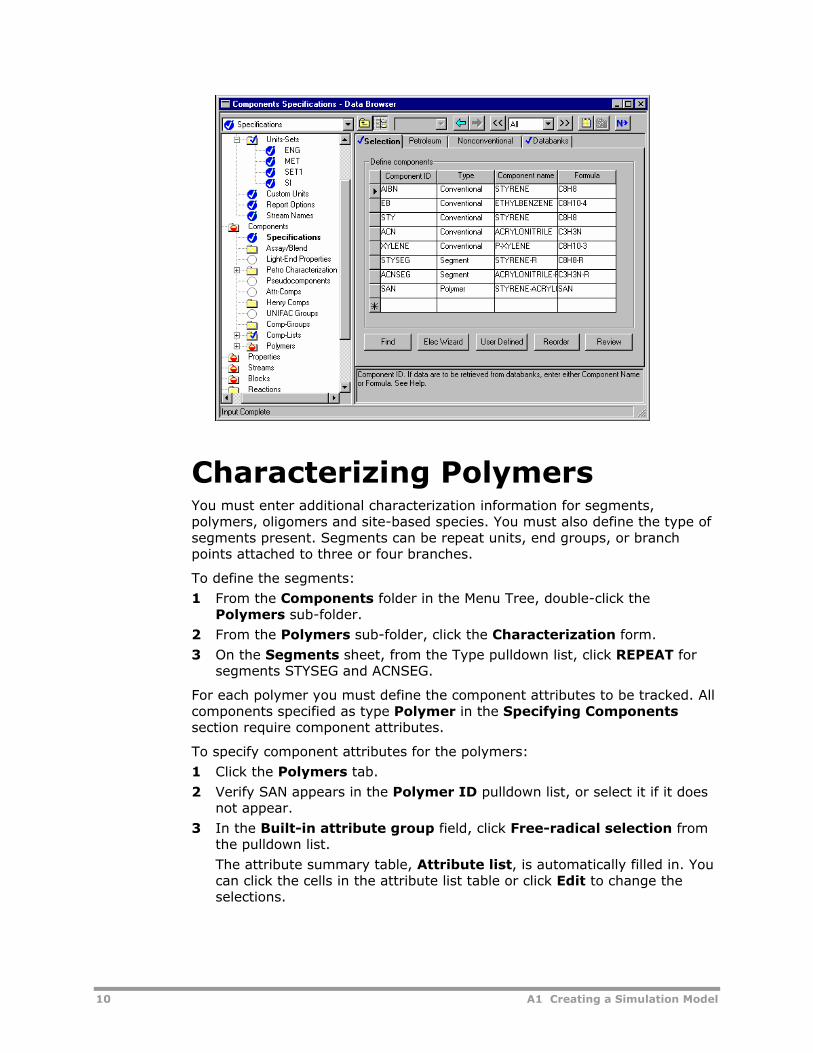
Specifying Components You use Components forms to select chemical components for your simulation and specify component types (for example, conventional, solid, assay, blend, polymer, segment, oligomer, and pseudocomponent).
To select components:
1 From the Data menu, click Components.
2 On the Selection sheet, enter the components as shown:
10 A1 Creating a Simulation Model
Characterizing Polymers You must enter additional characterization information for segments, polymers, oligomers and site-based species. You must also define the type of segments present. Segments can be repeat units, end groups, or branch points attached to three or four branches.
To define the segments:
1 From the Components folder in the Menu Tree, double-click the Polymers sub-folder.
2 From the Polymers sub-folder, click the Characterization form.
3 On the Segments sheet, from the Type pulldown list, click REPEAT for segments STYSEG and ACNSEG.
For each polymer you must define the component attributes to be tracked. All components specified as type Polymer in the Specifying Components section require component attributes.
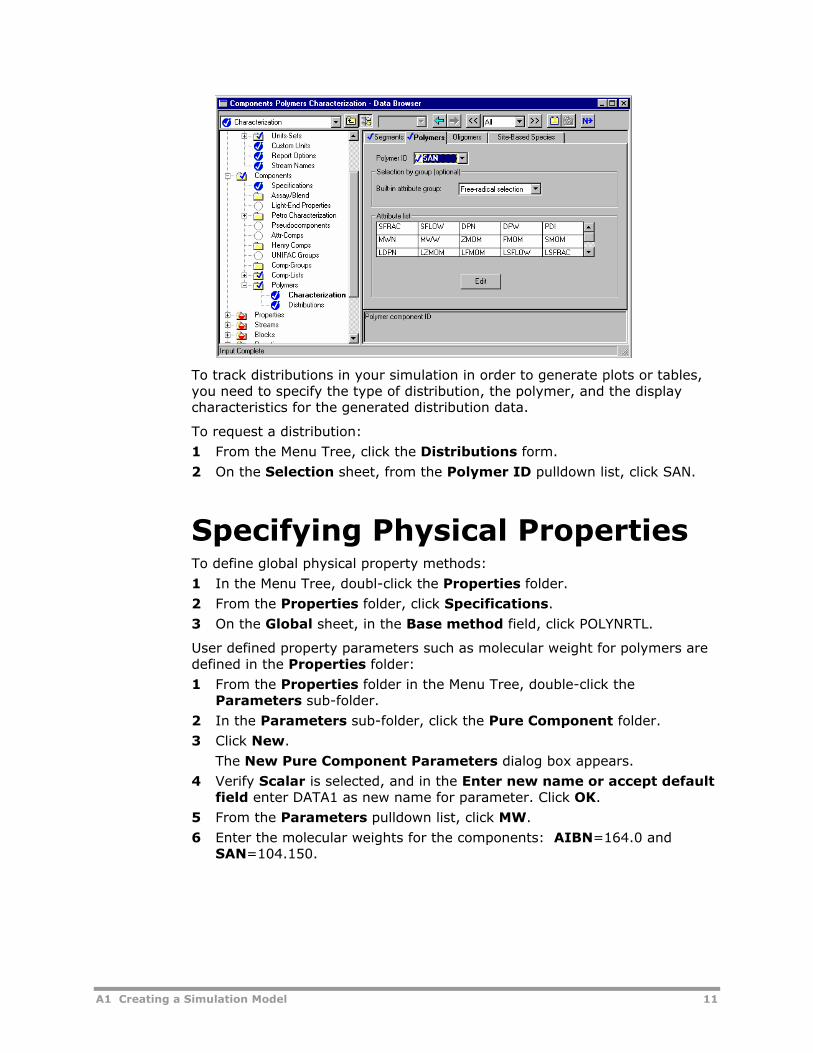
To specify component attributes for the polymers:
1 Click the Polymers tab.
2 Verify SAN appears in the Polymer ID pulldown list, or select it if it does not appear.
3 In the Built-in attribute group field, click Free-radical selection from the pulldown list.
The attribute summary table, Attribute list, is automatically filled in. You can click the cells in the attribute list table or click Edit to change the selections.
A1 Creating a Simulation Model 11
To track distributions in your simulation in order to generate plots or tables, you need to specify the type of distribution, the polymer, and the display characteristics for the generated distribution data.
To request a distribution:
1 From the Menu Tree, click the Distributions form.
2 On the Selection sheet, from the Polymer ID pulldown list, click SAN.
Specifying Physical Properties To define global physical property methods:
1 In the Menu Tree, doubl-click the Properties folder.
2 From the Properties folder, click Specifications.
3 On the Global sheet, in the Base method field, click POLYNRTL.
User defined property parameters such as molecular weight for polymers are defined in the Properties folder:
1 From the Properties folder in the Menu Tree, double-click the Parameters sub-folder.
2 In the Parameters sub-folder, click the Pure Component folder.
3 Click New.
The New Pure Component Parameters dialog box appears.
4 Verify Scalar is selected, and in the Enter new name or accept default field enter DATA1 as new name for parameter. Click OK.
5 From the Parameters pulldown list, click MW.
6 Enter the molecular weights for the components: AIBN=164.0 and SAN=104.150.
12 A1 Creating a Simulation Model
Specifying Feed Streams To enter stream specifications, you either open input forms from the Data Browser Menu Tree, or select a stream on the Process Flowsheet window and use the right mouse button to open the stream menu, where you click Input to open the input form. Here, you use the Menu Tree.
To enter feed stream specifications:
1 From the Menu Tree, double-click the Streams folder.
2 From the Streams folder, double-click the FEEDA sub-folder.
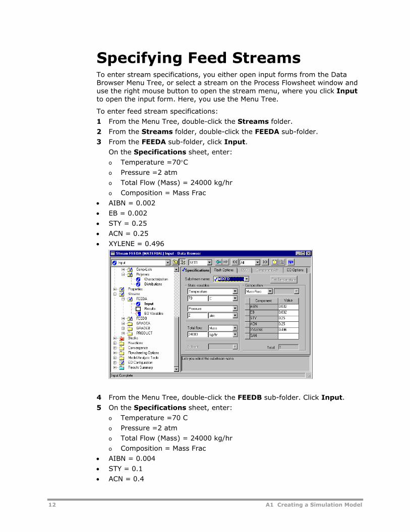
3 From the FEEDA sub-folder, click Input. On the Specifications sheet, enter:
o Temperature =70°C
o Pressure =2 atm
o Total Flow (Mass) = 24000 kg/hr
o Composition = Mass Frac
• AIBN = 0.002
• EB = 0.002
• STY = 0.25
• ACN = 0.25
• XYLENE = 0.496
4 From the Menu Tree, double-click the FEEDB sub-folder. Click Input.
5 On the Specifications sheet, enter: o Temperature =70 C
o Pressure =2 atm
o Total Flow (Mass) = 24000 kg/hr
o Composition = Mass Frac
• AIBN = 0.004
• STY = 0.1
• ACN = 0.4
A1 Creating a Simulation Model 13
• XYLENE = 0.496
Specifying Kinetics Kinetic inputs are specified in the Reactions folder. This example uses the free-radical kinetics model.
To specify the free-radical polymerization inputs:
1 From the Menu Tree, double-click the Reactions folder.
2 From the Reactions folder, click the Reactions sub-folder.
3 Click New to create a new reaction.
4 In the Enter ID field, type R1, in the Select type field, select FREE-RAD. Click OK.
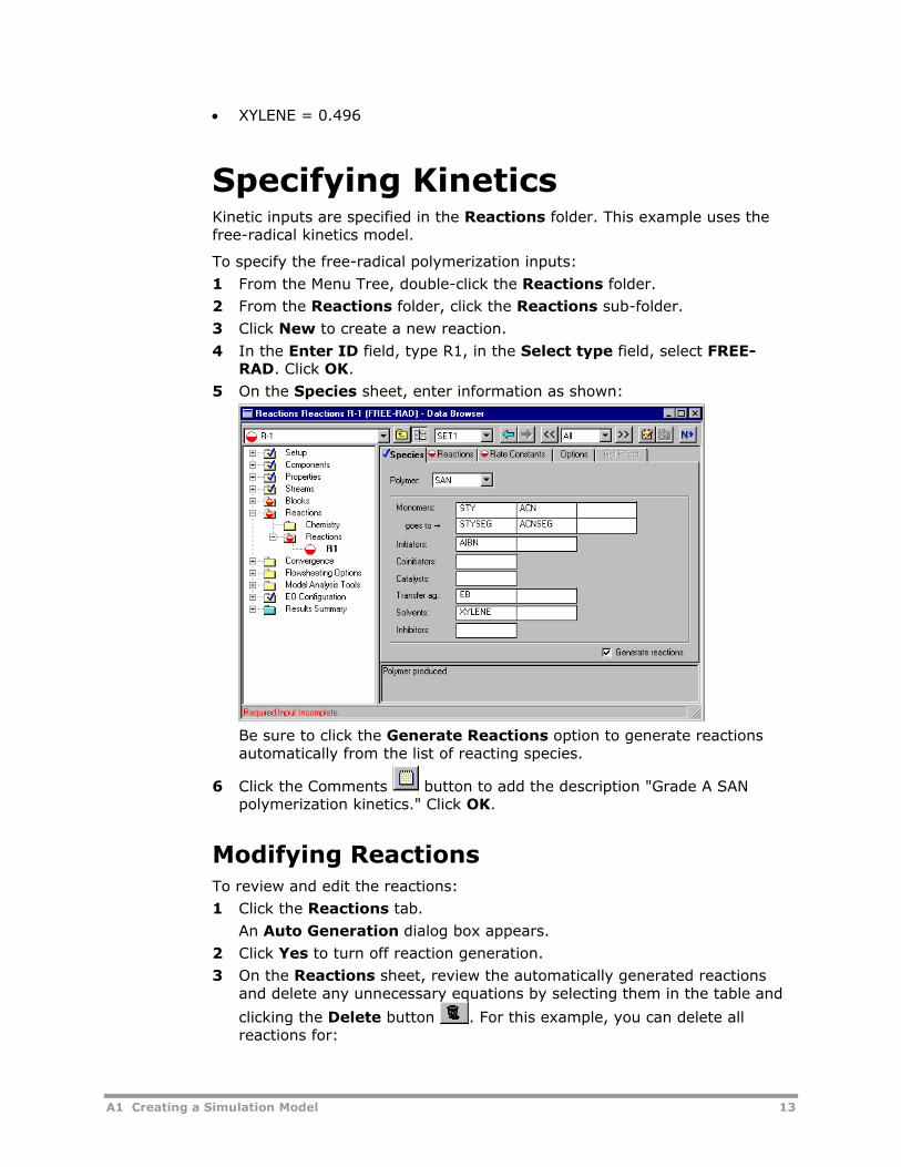
5 On the Species sheet, enter information as shown:
Be sure to click the Generate Reactions option to generate reactions automatically from the list of reacting species.
6 Click the Comments button to add the description "Grade A SAN polymerization kinetics." Click OK.
Modifying Reactions To review and edit the reactions:
1 Click the Reactions tab.
An Auto Generation dialog box appears.
2 Click Yes to turn off reaction generation.
3 On the Reactions sheet, review the automatically generated reactions and delete any unnecessary equations by selecting them in the table and
clicking the Delete button . For this example, you can delete all reactions for:
14 A1 Creating a Simulation Model
o Chat-agent
o Chat-sol
o Term-dis
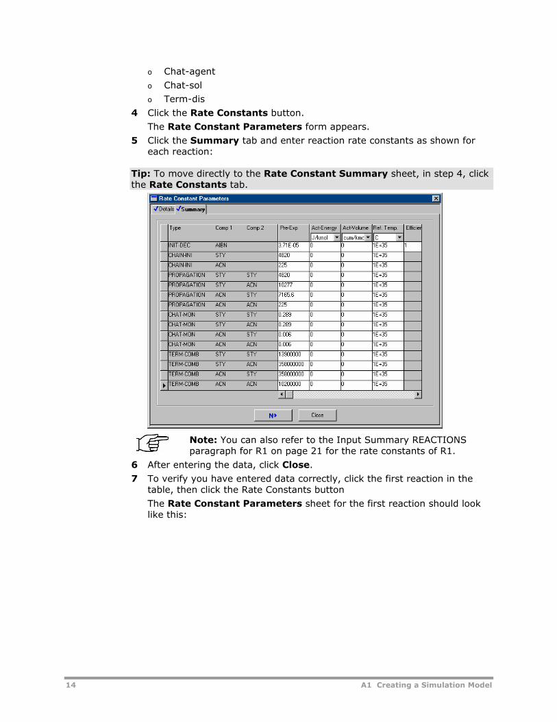
4 Click the Rate Constants button.
The Rate Constant Parameters form appears.
5 Click the Summary tab and enter reaction rate constants as shown for each reaction:
Tip: To move directly to the Rate Constant Summary sheet, in step 4, click the Rate Constants tab.
Note: You can also refer to the Input Summary REACTIONS paragraph for R1 on page 21 for the rate constants of R1.
6 After entering the data, click Close.
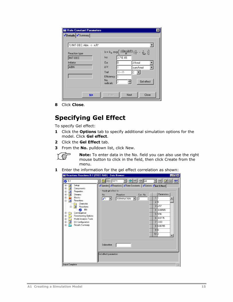
7 To verify you have entered data correctly, click the first reaction in the table, then click the Rate Constants button
The Rate Constant Parameters sheet for the first reaction should look like this:
A1 Creating a Simulation Model 15
8 Click Close.
Specifying Gel Effect To specify Gel effect:
1 Click the Options tab to specify additional simulation options for the model. Click Gel effect.
2 Click the Gel Effect tab.
3 From the No. pulldown list, click New.
Note: To enter data in the No. field you can also use the right mouse button to click in the field, then click Create from the menu.
1 Enter the information for the gel effect correlation as shown:
16 A1 Creating a Simulation Model
Repeat the above procedures for Specifying Kinetics, Modifying Reactions, and Specifying Gel Effect to specify the kinetics for R2. Refer to the Input Summary REACTIONS paragraph for R2 on page 21 for the appropriate comment, reactions, rate constants, and gel-effect correlations.
Defining the Unit Operation Block You must define the operating conditions for unit operations.
Entering Block Specifications To enter block specifications for the CSTR reactors:
1 From the Menu Tree, double-click the Blocks folder.
2 From the Blocks folder, double-click the B1 sub-folder.
3 Click Setup, and on the Specifications sheet enter:
o Pressure =2 atm
o Temperature =70 C
o Valid Phases = Liquid-Only
o Reactor Volume = 10 cum
4 Click the Reactions tab.
5 Click R1, then the button to move it from the Available Reaction Sets to the Selected Reaction Sets frame.
This defines R1 as the reaction set that describes the chemical reactions occurring in B1.
6 Click the Component Attr. tab and set: o Substream ID = MIXED
o Component ID = SAN
7 Enter a series of Attribute ID and Component Attribute values as below:
o Attribute ID = LPFRAC Component Attribute value = 1E-005
o Attribute ID = LEFRAC Component Attribute values = 0.5, 0.5
o Attribute ID = LSFRAC Component Attribute values = 0.5, 0.5
o Attribute ID = LDPN Component Attribute value = 500
o Attribute ID = SFRAC Component Attribute values = 0.5, 0.5
o Attribute ID = PDI Component Attribute value = 1.5
o Attribute ID = DPN Component Attribute value = 1000

A1 Creating a Simulation Model 17
Improving Convergence Polymer reaction kinetics present very difficult convergence problems, so the standard convergence options are frequently insufficient. To resolve this problem, we use the RCSTR block Convergence form. To do this:
1 From Blocks folder, B1 sub-folder in the Menu Tree, click the Convergence form.
2 Click the Parameters tab and change the Solver to Newton.
3 Click Newton Parameters and change the Stabilization Strategy to Line-Search. Click Close.
Note: This combination of parameters (step 2 and step 3) is recommended for all addition polymerization kinetics.
4 From the Parameters sheet, click Advanced Parameters and change the Scaling method to Component-based.
Note: Component-based scaling is recommended for all Aspen Polymers Plus simulations.
5 Click the Initialize using integration option.
When this option is selected, CSTR uses an integrator to provide an initial guess to the simultaneous equation solver.
Overriding Global Values Block Options forms can be used to override global values for physical properties, simulation options, diagnostic message levels and report options. For B1 the control panel diagnostic message level is set higher than the global default value 4. To override values:
1 From Blocks folder, BI sub-folder in the Menu Tree, click the Block Options form.
2 Click the Diagnostics tab, and set the On Screen slider bar to level 7.
Repeat the above procedures for Entering Block Specifications, Improving Convergence, and Overriding Global Values to define the unit operation block B2. Refer to the Input Summary BLOCKS B2 paragraph on page 20. Note that only the Convergence component values differ from Block B1.
Entering Mixer Specifications To enter Mixer specifications:
1 From the Blocks folder in Menu Tree, double-click the M sub-folder.
2 From the M sub-folder, click Input. 3 On the Flash Options sheet enter:
o Pressure = 1 atm
o Valid phases = Liquid-Only
18 A1 Creating a Simulation Model
Running the Simulation To run a simulation:
1 Click the button to confirm that you have finished entering all required input.
The Required Input Complete dialog box appears.
2 Click OK. A Control Panel appears, and shows the run progress.
Note: You can also open a control panel from the Aspen Plus toolbar, by
clicking the button, then the button.
As the run proceeds, status messages appear in the Control Panel. When the calculations are complete, the message Results Available appears in the status bar at the right corner of the Aspen Plus main window.
Examining Simulation Results When the message Results Available appears in the status bar you can examine your simulation results.
To examine the results:
1 From the Menu Tree, double-click the Results Summary folder.
2 In the Results Summary folder, click Run Status.
The Summary sheet appears.
The Aspen Plus version, run starting time and run status are summarized on this sheet.
3 From the Results Summary folder, click Streams.
The Material sheet appears with the stream results.
Since you selected the Polymers with Metric Units Simulation Template, POLY_M is used as the stream result format and reports stream Temperature, Pressure, Average MW, and other results. Mass Flow, and Mass Fraction are reported based on the selections made in the Specifying Setup and Global Options section on page 7. You can click the scroll bar to review the stream results that are off the screen.
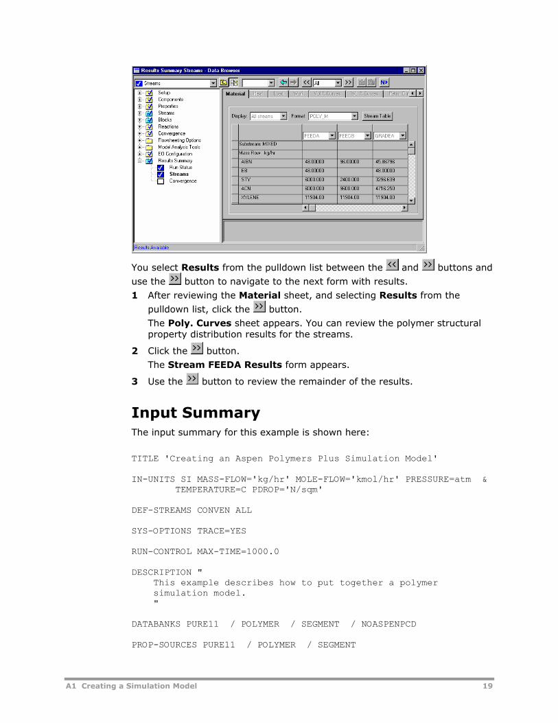
A1 Creating a Simulation Model 19
You select Results from the pulldown list between the and buttons and
use the button to navigate to the next form with results.
1 After reviewing the Material sheet, and selecting Results from the
pulldown list, click the button.
The Poly. Curves sheet appears. You can review the polymer structural property distribution results for the streams.
2 Click the button.
The Stream FEEDA Results form appears.
3 Use the button to review the remainder of the results.
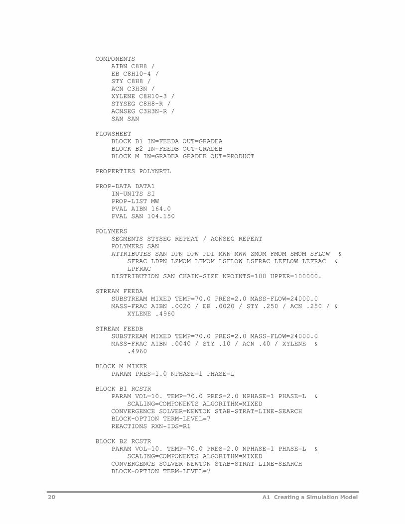
Input Summary The input summary for this example is shown here:
TITLE 'Creating an Aspen Polymers Plus Simulation Model' IN-UNITS SI MASS-FLOW='kg/hr' MOLE-FLOW='kmol/hr' PRESSURE=atm & TEMPERATURE=C PDROP='N/sqm' DEF-STREAMS CONVEN ALL SYS-OPTIONS TRACE=YES RUN-CONTROL MAX-TIME=1000.0 DESCRIPTION " This example describes how to put together a polymer simulation model. " DATABANKS PURE11 / POLYMER / SEGMENT / NOASPENPCD PROP-SOURCES PURE11 / POLYMER / SEGMENT
20 A1 Creating a Simulation Model
COMPONENTS AIBN C8H8 / EB C8H10-4 / STY C8H8 / ACN C3H3N / XYLENE C8H10-3 / STYSEG C8H8-R / ACNSEG C3H3N-R / SAN SAN FLOWSHEET BLOCK B1 IN=FEEDA OUT=GRADEA BLOCK B2 IN=FEEDB OUT=GRADEB BLOCK M IN=GRADEA GRADEB OUT=PRODUCT PROPERTIES POLYNRTL PROP-DATA DATA1 IN-UNITS SI PROP-LIST MW PVAL AIBN 164.0 PVAL SAN 104.150 POLYMERS SEGMENTS STYSEG REPEAT / ACNSEG REPEAT POLYMERS SAN ATTRIBUTES SAN DPN DPW PDI MWN MWW ZMOM FMOM SMOM SFLOW & SFRAC LDPN LZMOM LFMOM LSFLOW LSFRAC LEFLOW LEFRAC & LPFRAC DISTRIBUTION SAN CHAIN-SIZE NPOINTS=100 UPPER=100000. STREAM FEEDA SUBSTREAM MIXED TEMP=70.0 PRES=2.0 MASS-FLOW=24000.0 MASS-FRAC AIBN .0020 / EB .0020 / STY .250 / ACN .250 / & XYLENE .4960 STREAM FEEDB SUBSTREAM MIXED TEMP=70.0 PRES=2.0 MASS-FLOW=24000.0 MASS-FRAC AIBN .0040 / STY .10 / ACN .40 / XYLENE & .4960 BLOCK M MIXER PARAM PRES=1.0 NPHASE=1 PHASE=L BLOCK B1 RCSTR PARAM VOL=10. TEMP=70.0 PRES=2.0 NPHASE=1 PHASE=L & SCALING=COMPONENTS ALGORITHM=MIXED CONVERGENCE SOLVER=NEWTON STAB-STRAT=LINE-SEARCH BLOCK-OPTION TERM-LEVEL=7 REACTIONS RXN-IDS=R1 BLOCK B2 RCSTR PARAM VOL=10. TEMP=70.0 PRES=2.0 NPHASE=1 PHASE=L & SCALING=COMPONENTS ALGORITHM=MIXED CONVERGENCE SOLVER=NEWTON STAB-STRAT=LINE-SEARCH BLOCK-OPTION TERM-LEVEL=7
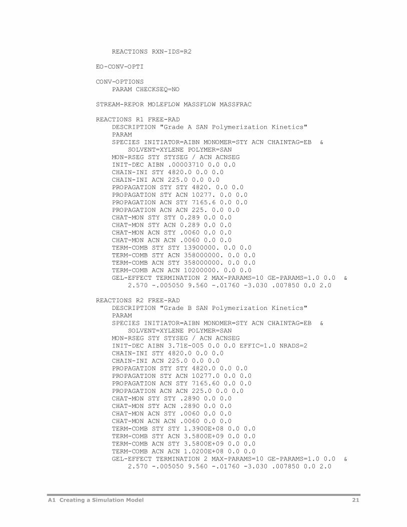
A1 Creating a Simulation Model 21
REACTIONS RXN-IDS=R2 EO-CONV-OPTI CONV-OPTIONS PARAM CHECKSEQ=NO STREAM-REPOR MOLEFLOW MASSFLOW MASSFRAC REACTIONS R1 FREE-RAD DESCRIPTION "Grade A SAN Polymerization Kinetics" PARAM SPECIES INITIATOR=AIBN MONOMER=STY ACN CHAINTAG=EB & SOLVENT=XYLENE POLYMER=SAN MON-RSEG STY STYSEG / ACN ACNSEG INIT-DEC AIBN .00003710 0.0 0.0 CHAIN-INI STY 4820.0 0.0 0.0 CHAIN-INI ACN 225.0 0.0 0.0 PROPAGATION STY STY 4820. 0.0 0.0 PROPAGATION STY ACN 10277. 0.0 0.0 PROPAGATION ACN STY 7165.6 0.0 0.0 PROPAGATION ACN ACN 225. 0.0 0.0 CHAT-MON STY STY 0.289 0.0 0.0 CHAT-MON STY ACN 0.289 0.0 0.0 CHAT-MON ACN STY .0060 0.0 0.0 CHAT-MON ACN ACN .0060 0.0 0.0 TERM-COMB STY STY 13900000. 0.0 0.0 TERM-COMB STY ACN 358000000. 0.0 0.0 TERM-COMB ACN STY 358000000. 0.0 0.0 TERM-COMB ACN ACN 10200000. 0.0 0.0 GEL-EFFECT TERMINATION 2 MAX-PARAMS=10 GE-PARAMS=1.0 0.0 & 2.570 -.005050 9.560 -.01760 -3.030 .007850 0.0 2.0 REACTIONS R2 FREE-RAD DESCRIPTION "Grade B SAN Polymerization Kinetics" PARAM SPECIES INITIATOR=AIBN MONOMER=STY ACN CHAINTAG=EB & SOLVENT=XYLENE POLYMER=SAN MON-RSEG STY STYSEG / ACN ACNSEG INIT-DEC AIBN 3.71E-005 0.0 0.0 EFFIC=1.0 NRADS=2 CHAIN-INI STY 4820.0 0.0 0.0 CHAIN-INI ACN 225.0 0.0 0.0 PROPAGATION STY STY 4820.0 0.0 0.0 PROPAGATION STY ACN 10277.0 0.0 0.0 PROPAGATION ACN STY 7165.60 0.0 0.0 PROPAGATION ACN ACN 225.0 0.0 0.0 CHAT-MON STY STY .2890 0.0 0.0 CHAT-MON STY ACN .2890 0.0 0.0 CHAT-MON ACN STY .0060 0.0 0.0 CHAT-MON ACN ACN .0060 0.0 0.0 TERM-COMB STY STY 1.3900E+08 0.0 0.0 TERM-COMB STY ACN 3.5800E+09 0.0 0.0 TERM-COMB ACN STY 3.5800E+09 0.0 0.0 TERM-COMB ACN ACN 1.0200E+08 0.0 0.0 GEL-EFFECT TERMINATION 2 MAX-PARAMS=10 GE-PARAMS=1.0 0.0 & 2.570 -.005050 9.560 -.01760 -3.030 .007850 0.0 2.0
22 A1 Creating a Simulation Model
Plotting Distributions Follow these instructions to:
• Display and plot the distribution data for a polymerization reactor
• Display a distribution table for a stream or an entire flowsheet
To display and plot the distribution data for a polymerization reactor:
1 From the Blocks folder B1 sub-folder in the Menu Tree, click the Results form.
2 Click the Distributions tab.
3 From the Aspen Plus menu bar, click Plot, then Plot Wizard.
The Aspen Plus Plot Wizard appears.
4 Click Next, then the icon for Chain Size Distr. plot type.
5 Click Next. If you want to review further plot options, click Next, or proceed directly to the next step.
6 Click Finish.
The plot is displayed.
Note: You can modify the plot by using the right mouse button to click the objects in the plot window. From the menu, click Edit, Properties, or Modify to make necessary changes.
To display a distribution table for a stream or for the entire flowsheet:
1 From the Menu Tree, double-click the Results Summary folder.
2 Click the Streams form.
3 Click the Poly. Curves tab. You may need to use the scroll arrows to locate the tab.
4 From the Aspen Plus menu bar, click Plot, then Plot Wizard.
5 Click Next, then the icon for Chain Size Distr. plot type.
6 Click Next.
7 Click the stream(s) you want to plot from the Available box and click the button to move them to the Selected box. In this example, all
streams are selected. If you want to review further plot options, click Next, or proceed directly to the next step.
8 Click Finish.
The plot appears.
A1 Creating a Simulation Model 23
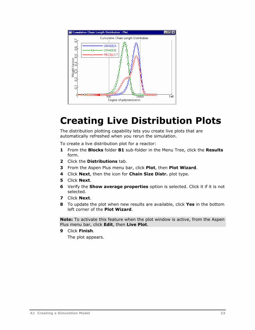
Creating Live Distribution Plots The distribution plotting capability lets you create live plots that are automatically refreshed when you rerun the simulation.
To create a live distribution plot for a reactor:
1 From the Blocks folder B1 sub-folder in the Menu Tree, click the Results form.
2 Click the Distributions tab.
3 From the Aspen Plus menu bar, click Plot, then Plot Wizard.
4 Click Next, then the icon for Chain Size Distr. plot type.
5 Click Next. 6 Verify the Show average properties option is selected. Click it if it is not
selected.
7 Click Next.
8 To update the plot when new results are available, click Yes in the bottom left corner of the Plot Wizard.
Note: To activate this feature when the plot window is active, from the Aspen Plus menu bar, click Edit, then Live Plot. 9 Click Finish.
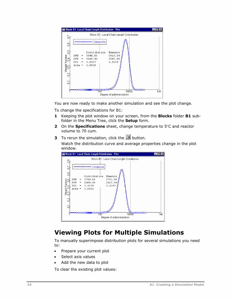
The plot appears.
24 A1 Creating a Simulation Model
You are now ready to make another simulation and see the plot change.
To change the specifications for B1:
1 Keeping the plot window on your screen, from the Blocks folder B1 sub-folder in the Menu Tree, click the Setup form.
2 On the Specifications sheet, change temperature to 5°C and reactor volume to 70 cum.
3 To rerun the simulation, click the button.
Watch the distribution curve and average properties change in the plot window.
Viewing Plots for Multiple Simulations To manually superimpose distribution plots for several simulations you need to:
• Prepare your current plot
• Select axis values
• Add the new data to plot
To clear the existing plot values:
A1 Creating a Simulation Model 25
1 Click to make the plot window active. From the Aspen Plus menu bar, click Edit, then Live Plot. This turns off the feature.
2 Click the average property text (DPN, DPW, PDI) on the plot, click the right mouse button, then Delete. Click OK.
3 From the Blocks folder B1 sub-folder in the Menu Tree, click the Setup form.
4 On the Specifications sheet, change temperature back to 70°C and reactor volume to 10 cum.
5 To run the simulation, click the button. This time the plot does not change.
To manually select x-axis and y-axis values for the plot:
1 From the Blocks folder B1 sub-folder in the Menu Tree, click the Results form.
2 Click the Distributions tab.
3 You are going to manually select the x-axis values and y-axis values for the new plot. Click DPn to select the degree of polymerization column as the x-axis.
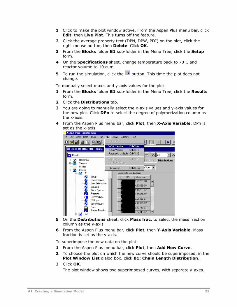
4 From the Aspen Plus menu bar, click Plot, then X-Axis Variable. DPn is set as the x-axis.
5 On the Distributions sheet, click Mass frac. to select the mass fraction
column as the y-axis.
6 From the Aspen Plus menu bar, click Plot, then Y-Axis Variable. Mass fraction is set as the y-axis.
To superimpose the new data on the plot:
1 From the Aspen Plus menu bar, click Plot, then Add New Curve.
2 To choose the plot on which the new curve should be superimposed, in the Plot Window List dialog box, click B1: Chain Length Distribution.
3 Click OK.
The plot window shows two superimposed curves, with separate y-axes.
26 A1 Creating a Simulation Model
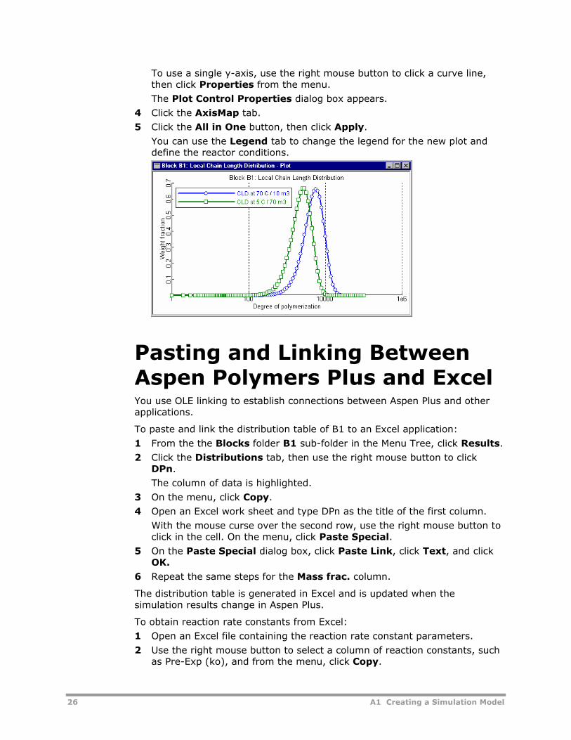
To use a single y-axis, use the right mouse button to click a curve line, then click Properties from the menu.
The Plot Control Properties dialog box appears.
4 Click the AxisMap tab.
5 Click the All in One button, then click Apply.
You can use the Legend tab to change the legend for the new plot and define the reactor conditions.
Pasting and Linking Between Aspen Polymers Plus and Excel You use OLE linking to establish connections between Aspen Plus and other applications.
To paste and link the distribution table of B1 to an Excel application:
1 From the the Blocks folder B1 sub-folder in the Menu Tree, click Results.
2 Click the Distributions tab, then use the right mouse button to click DPn.
The column of data is highlighted.
3 On the menu, click Copy.
4 Open an Excel work sheet and type DPn as the title of the first column.
With the mouse curse over the second row, use the right mouse button to click in the cell. On the menu, click Paste Special.
5 On the Paste Special dialog box, click Paste Link, click Text, and click OK.
6 Repeat the same steps for the Mass frac. column.
The distribution table is generated in Excel and is updated when the simulation results change in Aspen Plus.
To obtain reaction rate constants from Excel:
1 Open an Excel file containing the reaction rate constant parameters.
2 Use the right mouse button to select a column of reaction constants, such as Pre-Exp (ko), and from the menu, click Copy.
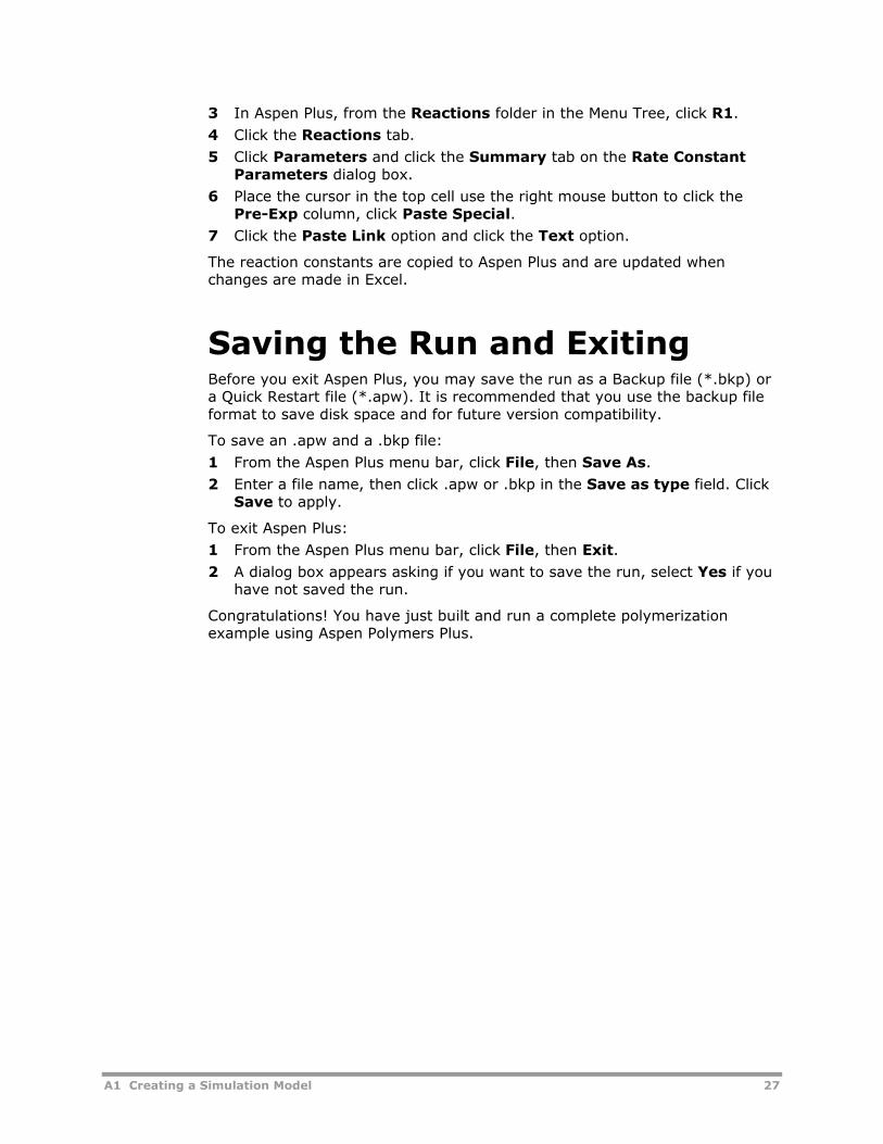
A1 Creating a Simulation Model 27
3 In Aspen Plus, from the Reactions folder in the Menu Tree, click R1.
4 Click the Reactions tab.
5 Click Parameters and click the Summary tab on the Rate Constant Parameters dialog box.
6 Place the cursor in the top cell use the right mouse button to click the Pre-Exp column, click Paste Special.
7 Click the Paste Link option and click the Text option.
The reaction constants are copied to Aspen Plus and are updated when changes are made in Excel.
Saving the Run and Exiting Before you exit Aspen Plus, you may save the run as a Backup file (*.bkp) or a Quick Restart file (*.apw). It is recommended that you use the backup file format to save disk space and for future version compatibility.
To save an .apw and a .bkp file:
1 From the Aspen Plus menu bar, click File, then Save As.
2 Enter a file name, then click .apw or .bkp in the Save as type field. Click Save to apply.
To exit Aspen Plus:
1 From the Aspen Plus menu bar, click File, then Exit.
2 A dialog box appears asking if you want to save the run, select Yes if you have not saved the run.
Congratulations! You have just built and run a complete polymerization example using Aspen Polymers Plus.

28 A2 Predicting Physical Properties
A2 Predicting Physical Properties
This example demonstrates how to use Aspen Polymers Plus to predict pure component properties of polymers using the Van Krevelen group contribution method.
The steps covered include:
• Defining the Simulation
• Creating a New Run
• Specifying Setup and Global Options
• Specifying and Characterizing Components
• Specifying Physical Properties
• Defining Molecular Structure
• Specifying Mass Fraction Crystallinity
• Creating Property Sets
• Creating Property Tables
• Running the Simulation and Examining the Results
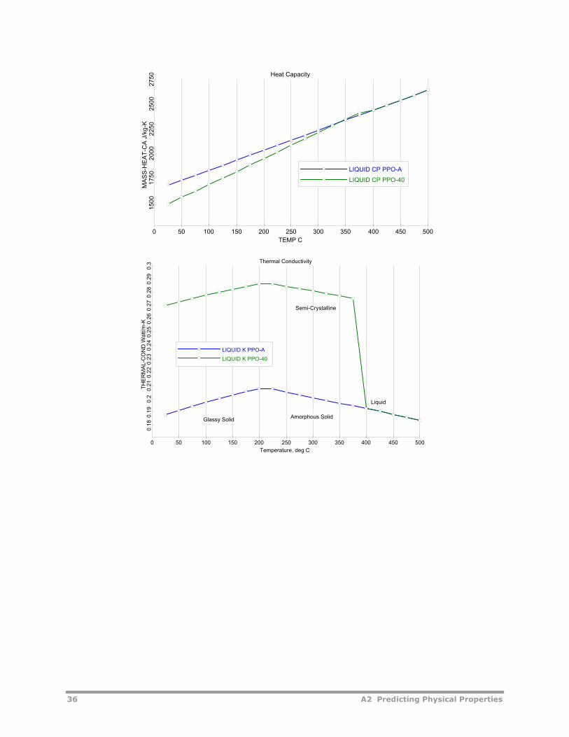
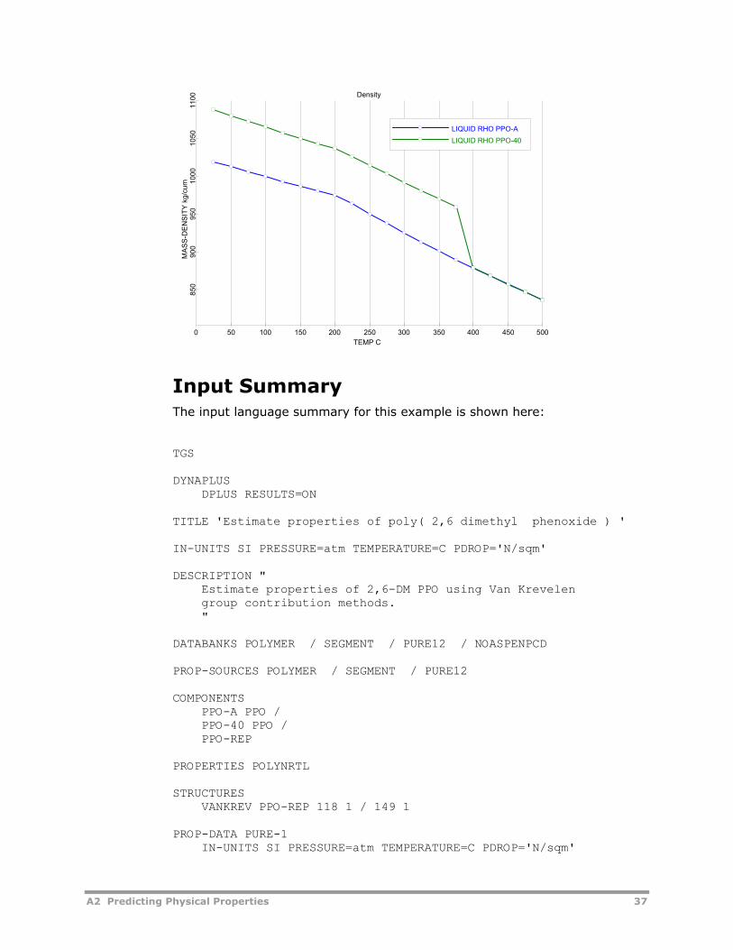
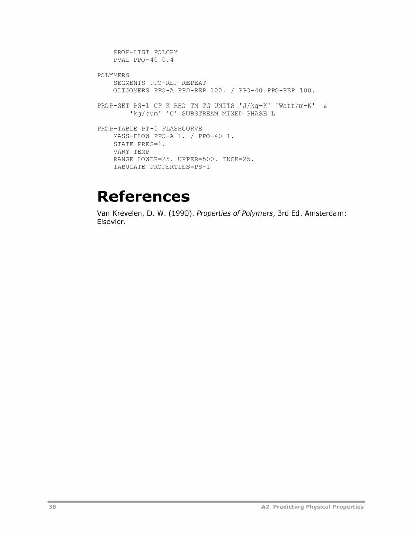
The Van Krevelen method is based on the chemical structure of the polymers (Van Krevelen, 1990) . It uses additive molar functions based on group contribution. Using this technique a variety of polymer properties can be predicted. In Aspen Polymers Plus, the Van Krevelen method is used to estimate heat capacity of both liquid and solid polymers, liquid viscosity and thermal conductivity for both polymer melt and polymer solution, and density. In this example, heat capacity, thermal conductivity, and density are predicted at atmospheric pressure in the temperature range of 20 to 500°C for poly (2,6 dimethyl phenylene oxide). Since this temperature range crosses the glass point and melting point of the polymer we will see predictions for liquid and solid polymer.
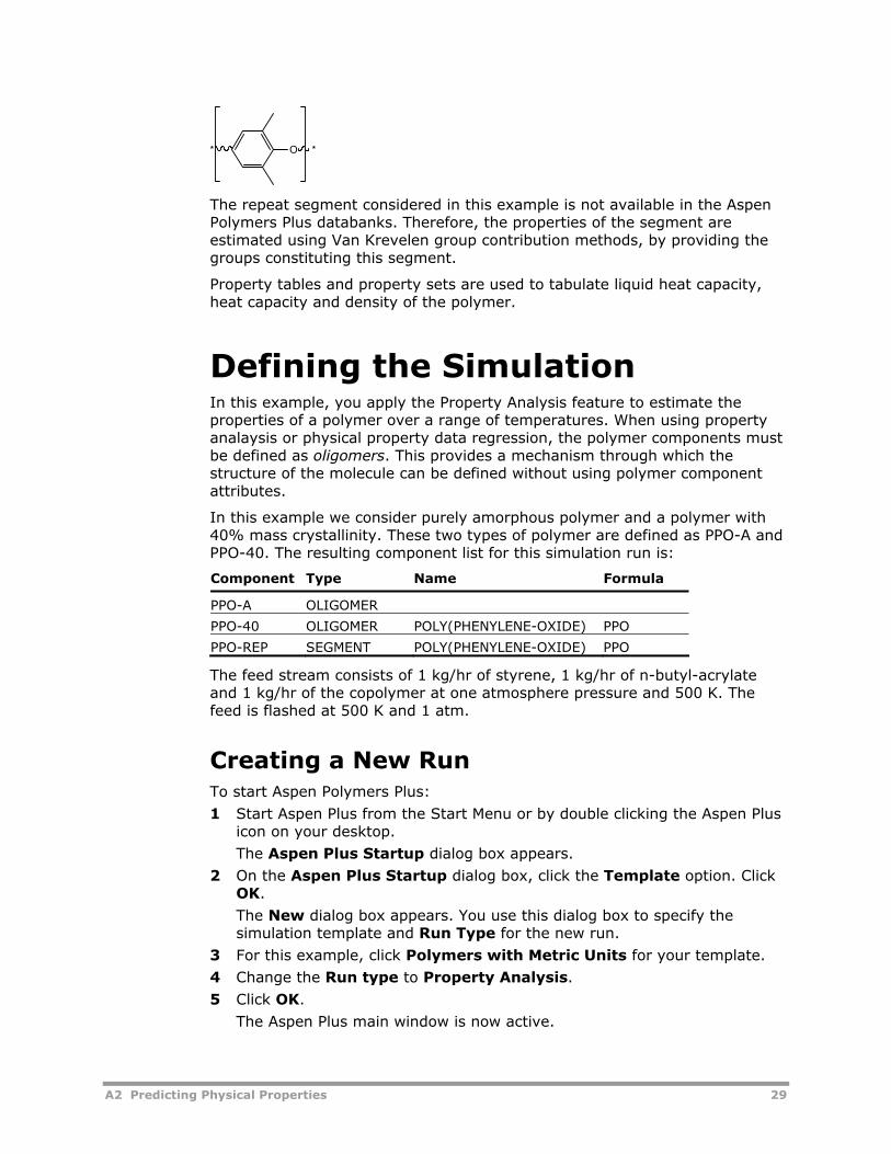
In this example, we consider the polymer of 2,6 dimethyl phenol, which can polymerize through an oxidative coupling reaction to form a type of poly(phenylene oxide), an aromatic polyether.
The structure of the repeat unit of this polymer is:
A2 Predicting Physical Properties 29
* O *
The repeat segment considered in this example is not available in the Aspen Polymers Plus databanks. Therefore, the properties of the segment are estimated using Van Krevelen group contribution methods, by providing the groups constituting this segment.
Property tables and property sets are used to tabulate liquid heat capacity, heat capacity and density of the polymer.
Defining the Simulation In this example, you apply the Property Analysis feature to estimate the properties of a polymer over a range of temperatures. When using property analaysis or physical property data regression, the polymer components must be defined as oligomers. This provides a mechanism through which the structure of the molecule can be defined without using polymer component attributes.
In this example we consider purely amorphous polymer and a polymer with 40% mass crystallinity. These two types of polymer are defined as PPO-A and PPO-40. The resulting component list for this simulation run is:
Component Type Name Formula
PPO-A OLIGOMER
PPO-40 OLIGOMER POLY(PHENYLENE-OXIDE) PPO
PPO-REP SEGMENT POLY(PHENYLENE-OXIDE) PPO
The feed stream consists of 1 kg/hr of styrene, 1 kg/hr of n-butyl-acrylate and 1 kg/hr of the copolymer at one atmosphere pressure and 500 K. The feed is flashed at 500 K and 1 atm.
Creating a New Run To start Aspen Polymers Plus:
1 Start Aspen Plus from the Start Menu or by double clicking the Aspen Plus icon on your desktop.
The Aspen Plus Startup dialog box appears.
2 On the Aspen Plus Startup dialog box, click the Template option. Click OK.
The New dialog box appears. You use this dialog box to specify the simulation template and Run Type for the new run.
3 For this example, click Polymers with Metric Units for your template.
4 Change the Run type to Property Analysis.
5 Click OK.
The Aspen Plus main window is now active.
30 A2 Predicting Physical Properties
Note: For convenience, you may wish to change the default units set to use temperature in degree C.
You are now ready to enter input data for your simulation.
Specifying Setup and Global Options To enter process and model specifications into Aspen Polymers Plus, you can
use the Next button or the Data Browser Menu Tree. In this example, you
enter data using button.
To enter a title and description for the simulation:
1 From the Aspen Plus toolbar, click the button.
The Setup Specifications - Data Browser appears.
2 On the Global sheet, type the title of your simulation run as: Estimate properties of poly(2,6 dimethyl phenoxide)
3 Click the Description tab.
You can either retain or delete the default information displayed, but type the following description: Estimate properties of 2,6-DM PPO using Van Krevelen group contribution methods.
4 Click .
A Component Specifications Selection sheet appears.
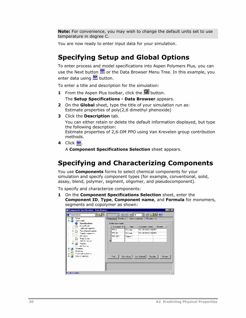
Specifying and Characterizing Components You use Components forms to select chemical components for your simulation and specify component types (for example, conventional, solid, assay, blend, polymer, segment, oligomer, and pseudocomponent).
To specify and characterize components:
1 On the Component Specifications Selection sheet, enter the Component ID, Type, Component name, and Formula for monomers, segments and copolymer as shown:
A2 Predicting Physical Properties 31
Note: For the segment PPO-REP, the name and formula slots are left empty because as part of this exercise you will provide molecular structure for this segment.
2 Click .
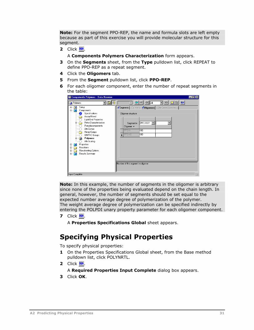
A Components Polymers Characterization form appears.
3 On the Segments sheet, from the Type pulldown list, click REPEAT to define PPO-REP as a repeat segment.
4 Click the Oligomers tab.
5 From the Segment pulldown list, click PPO-REP.
6 For each oligomer component, enter the number of repeat segments in the table:
Note: In this example, the number of segments in the oligomer is arbitrary since none of the properties being evaluated depend on the chain length. In general, however, the number of segments should be set equal to the expected number average degree of polymerization of the polymer. The weight average degree of polymerization can be specified indirectly by entering the POLPDI unary property parameter for each oligomer component.
7 Click .
A Properties Specifications Global sheet appears.
Specifying Physical Properties To specify physical properties:
1 On the Properties Specifications Global sheet, from the Base method pulldown list, click POLYNRTL.
2 Click .
A Required Properties Input Complete dialog box appears.
3 Click OK.
32 A2 Predicting Physical Properties
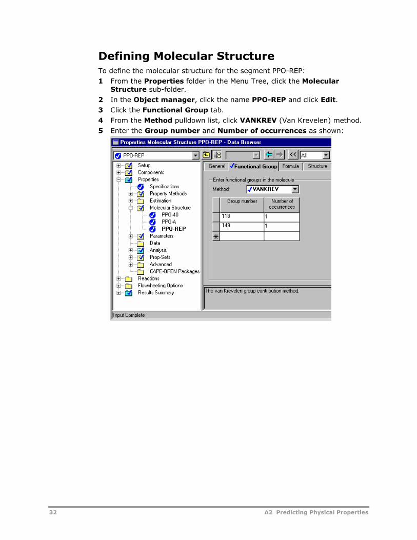
Defining Molecular Structure To define the molecular structure for the segment PPO-REP:
1 From the Properties folder in the Menu Tree, click the Molecular Structure sub-folder.
2 In the Object manager, click the name PPO-REP and click Edit. 3 Click the Functional Group tab.
4 From the Method pulldown list, click VANKREV (Van Krevelen) method.
5 Enter the Group number and Number of occurrences as shown:
A2 Predicting Physical Properties 33
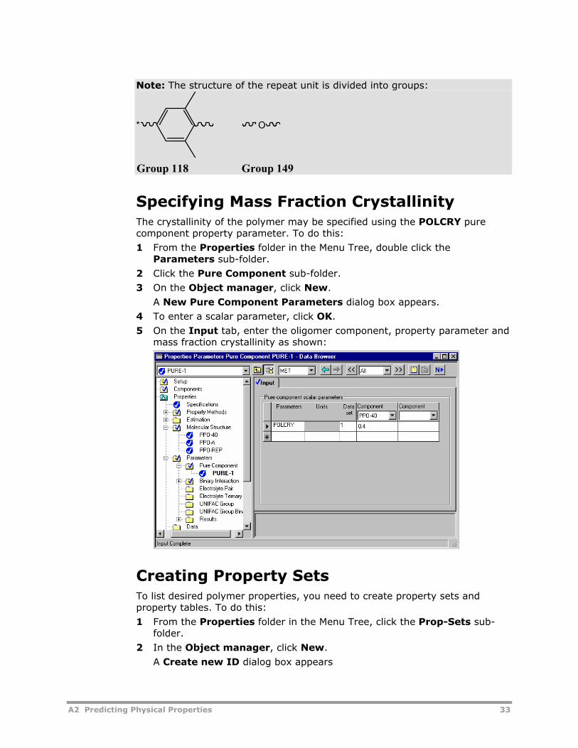
Note: The structure of the repeat unit is divided into groups:
* O
Group 118 Group 149
Specifying Mass Fraction Crystallinity The crystallinity of the polymer may be specified using the POLCRY pure component property parameter. To do this:
1 From the Properties folder in the Menu Tree, double click the Parameters sub-folder.
2 Click the Pure Component sub-folder.
3 On the Object manager, click New.
A New Pure Component Parameters dialog box appears.
4 To enter a scalar parameter, click OK.
5 On the Input tab, enter the oligomer component, property parameter and mass fraction crystallinity as shown:
Creating Property Sets To list desired polymer properties, you need to create property sets and property tables. To do this:
1 From the Properties folder in the Menu Tree, click the Prop-Sets sub-folder.
2 In the Object manager, click New.
A Create new ID dialog box appears
34 A2 Predicting Physical Properties
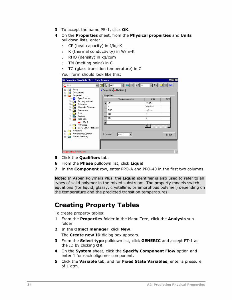
3 To accept the name PS-1, click OK.
4 On the Properties sheet, from the Physical properties and Units pulldown lists, enter:
o CP (heat capacity) in J/kg-K
o K (thermal conductivity) in W/m-K
o RHO (density) in kg/cum
o TM (melting point) in C
o TG (glass transition temperature) in C
Your form should look like this:
5 Click the Qualifiers tab.
6 From the Phase pulldown list, click Liquid
7 In the Component row, enter PPO-A and PPO-40 in the first two columns.
Note: In Aspen Polymers Plus, the Liquid identifier is also used to refer to all types of solid polymer in the mixed substream. The property models switch equations (for liquid, glassy, crystalline, or amorphous polymer) depending on the temperature and the predicted transition temperatures.
Creating Property Tables To create property tables:
1 From the Properties folder in the Menu Tree, click the Analysis sub-folder.
2 In the Object manager, click New.
The Create new ID dialog box appears.
3 From the Select type pulldown list, click GENERIC and accept PT-1 as the ID by clicking OK.
4 On the System sheet, click the Specify Component Flow option and enter 1 for each oligomer component.
5 Click the Variable tab, and for Fixed State Variables, enter a pressure of 1 atm.
A2 Predicting Physical Properties 35
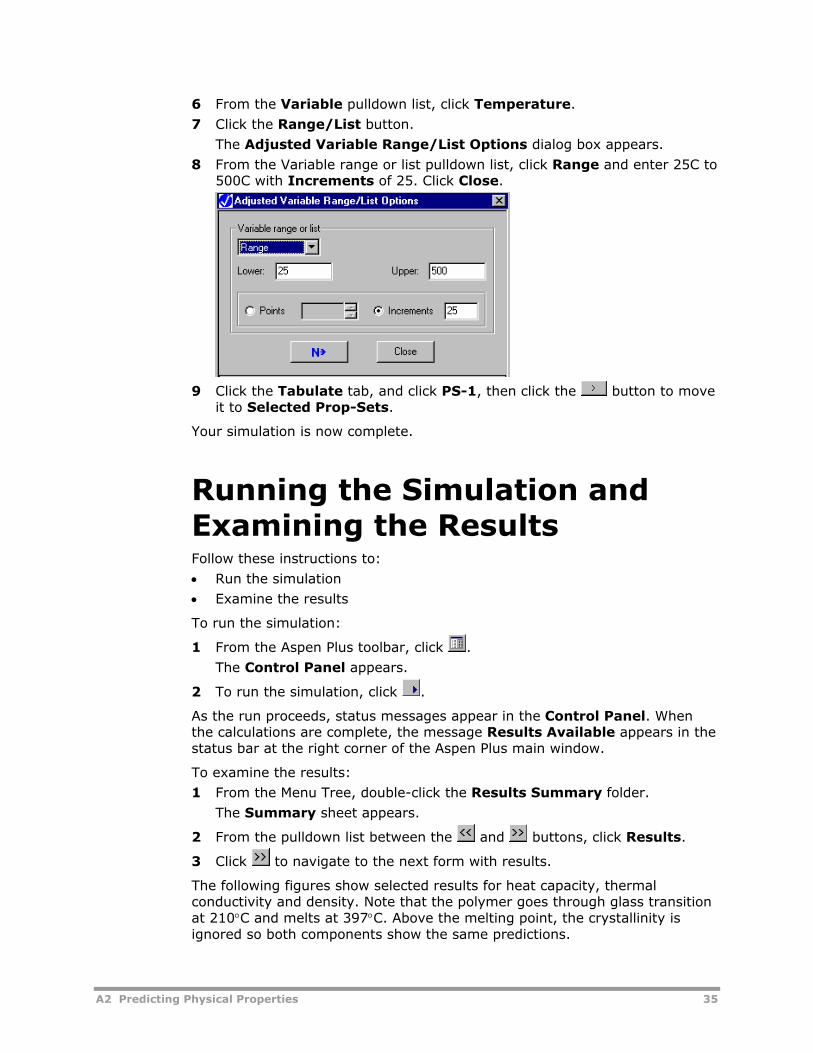
6 From the Variable pulldown list, click Temperature.
7 Click the Range/List button.
The Adjusted Variable Range/List Options dialog box appears.
8 From the Variable range or list pulldown list, click Range and enter 25C to 500C with Increments of 25. Click Close.
9 Click the Tabulate tab, and click PS-1, then click the button to move
it to Selected Prop-Sets.
Your simulation is now complete.
Running the Simulation and Examining the Results Follow these instructions to:
• Run the simulation
• Examine the results
To run the simulation:
1 From the Aspen Plus toolbar, click .
The Control Panel appears.
2 To run the simulation, click .
As the run proceeds, status messages appear in the Control Panel. When the calculations are complete, the message Results Available appears in the status bar at the right corner of the Aspen Plus main window.
To examine the results:
1 From the Menu Tree, double-click the Results Summary folder.
The Summary sheet appears.
2 From the pulldown list between the and buttons, click Results.
3 Click to navigate to the next form with results.
The following figures show selected results for heat capacity, thermal conductivity and density. Note that the polymer goes through glass transition at 210°C and melts at 397°C. Above the melting point, the crystallinity is ignored so both components show the same predictions.
36 A2 Predicting Physical Properties
Heat Capacity
TEMP C
MA
SS
-HE
AT-
CA
J/k
g-K
0 50 100 150 200 250 300 350 400 450 500
1500
1750
2000
2250
2500
2750
LIQUID CP PPO-A
LIQUID CP PPO-40
Thermal Conductivity
Temperature, deg C
THE
RM
AL-
CO
ND
Wat
t/m-K
0 50 100 150 200 250 300 350 400 450 500
0.18
0.19
0.2
0.21
0.22
0.23
0.24
0.25
0.26
0.27
0.28
0.29
0.3
LIQUID K PPO-ALIQUID K PPO-40
Liquid
Amorphous SolidGlassy Solid
Semi-Crystalline
A2 Predicting Physical Properties 37
Density
TEMP C
MA
SS
-DE
NS
ITY
kg/
cum
0 50 100 150 200 250 300 350 400 450 500
850
900
950
1000
1050
1100
LIQUID RHO PPO-ALIQUID RHO PPO-40
Input Summary The input language summary for this example is shown here:
TGS DYNAPLUS DPLUS RESULTS=ON TITLE 'Estimate properties of poly( 2,6 dimethyl phenoxide ) ' IN-UNITS SI PRESSURE=atm TEMPERATURE=C PDROP='N/sqm' DESCRIPTION " Estimate properties of 2,6-DM PPO using Van Krevelen group contribution methods. " DATABANKS POLYMER / SEGMENT / PURE12 / NOASPENPCD PROP-SOURCES POLYMER / SEGMENT / PURE12 COMPONENTS PPO-A PPO / PPO-40 PPO / PPO-REP PROPERTIES POLYNRTL STRUCTURES VANKREV PPO-REP 118 1 / 149 1 PROP-DATA PURE-1 IN-UNITS SI PRESSURE=atm TEMPERATURE=C PDROP='N/sqm'
38 A2 Predicting Physical Properties
PROP-LIST POLCRY PVAL PPO-40 0.4 POLYMERS SEGMENTS PPO-REP REPEAT OLIGOMERS PPO-A PPO-REP 100. / PPO-40 PPO-REP 100. PROP-SET PS-1 CP K RHO TM TG UNITS='J/kg-K' 'Watt/m-K' & 'kg/cum' 'C' SUBSTREAM=MIXED PHASE=L PROP-TABLE PT-1 FLASHCURVE MASS-FLOW PPO-A 1. / PPO-40 1. STATE PRES=1. VARY TEMP RANGE LOWER=25. UPPER=500. INCR=25. TABULATE PROPERTIES=PS-1
References Van Krevelen, D. W. (1990). Properties of Polymers, 3rd Ed. Amsterdam: Elsevier.
A3 Regressing Property Parameters 39
A3 Regressing Property Parameters
This example demonstrates how to use the data regression (DRS) capabilities to fit the mixture parameters of an equation of state (EOS) model to binary vapor-liquid equilibrium (VLE) data.
The steps covered include:
• Defining the Simulation
• Creating a New Run
• Specifying Setup and Global Options
• Specifying and Characterizing Components
• Specifying Physical Property Method
• Entering Experimental Data
• Specifying a Regression Case
• Specifying Physical Property Parameters
• Running the Simulation and Examining the Results
Correlative models used to describe thermodynamic properties of mixtures often contain binary interaction parameters. These parameters account for mixture non-idealities, and are necessary for accurate representation of the mixture behavior. For each constituent pair of a multicomponent mixture, these parameters are obtained by regressing some form of binary experimental information.
In this example, binary VLE data of ethylene-polyethylene mixture is regressed to obtain the two binary interaction parameters of the Sanchez-Lacombe EOS, and . You can find the details of this model in Volume 2
of the Aspen Polymers Plus User Guide. Ethylene-polyethylene binary mixture is encountered in polyolefin production, and at high pressures the thermodynamic behavior of this mixture can be described by an EOS such as the Sanchez-Lacombe model.
40 A3 Regressing Property Parameters
Defining the Simulation In this example, you create an Aspen Polymers Plus data regression (DRS) session, run the DRS, and examine the results.
Creating a New Run To start Aspen Polymers Plus:
1 Start Aspen Plus from the Start Menu or by double clicking the Aspen Plus icon on your desktop.
The Aspen Plus Startup dialog box appears.
2 On the Aspen Plus Startup dialog box, click the Template option. Click OK.
The New dialog box appears. You use this dialog box to specify the simulation template and Run Type for the new run. Aspen Plus uses the Simulation Template you choose to automatically set various defaults appropriate to your application.
3 For this example, click Polymers with Metric Units for your template.
4 From the Run type pulldown list, click Data Regression
5 Click OK.
The Aspen Plus main window is now active.
Specifying Setup and Global Options To enter process and model specifications into Aspen Polymers Plus, you can
use the Next button or the Data Browser Menu Tree. In this example, you
enter data using button.
User the Setup folder to:
• Enter simulation title and description
• Define unit-sets
Entering a Simulation Title and Description To enter a title and description for the simulation:
1 From the Aspen Plus toolbar, click .
The Setup Specifications - Data Browser appears.
2 On the Global sheet, type the title of your simulation run as: Regression of binary parameters for the POLYSL model
3 In the Units of measurement field, for Input data and Output results, click SI.
4 Click the Description tab.
You can either retain or delete the default information displayed, but type the following description: The objective of this example is to demonstrate how to use the data
A3 Regressing Property Parameters 41
regression capabilities to fit the mixture parameters of an EOS model to binary VLE data.
Defining Unit-Sets To define a unit-set:
1 From the Setup folder in the Menu Tree, click the Units-Sets sub-folder.
2 Click New.
3 To accept US-1 as the unit set ID, click OK.
A dialog box appears requesting approval to make US-1 the global unit set
4 Click No.
5 On the Standard sheet, from the Copy from pulldown list, click Eng.
6 Set the following options:
o Temperature = K
o Pressure = bar
7 Click the Transport tab
8 From the Density pulldown list, click kg/cum.
9 Repeat these steps to create unit set US-3 (step 3) in which:
o Copy from=SI (step 5)
o Pressure=bar (step 6)
o Delta P=bar (step 6)
10 Click .
A Component Specifications Selection sheet appears.
Specifying and Characterizing Components The component information necessary for this DRS run is:
Component ID
Type Component Name Formula
PE Oligomer POLY(ETHYLENE) PE
ETHYLENE Conventional ETHYLENE C2H4
C2H4-R Segment ETHYLENE-R C2H4-R
In this example, the polymer is identified as oligomer. This is required for property data regresssion and property analysis runs. By defining the polymer as an oligomer, the need to enter any attribute information is eliminated.
The composition (segment fractions) and the number-average chain length and moleuclar weight of the polymer are determined from the structure defined in the oligomer form. To avoid a warning message, you need to supply the true molecular weight of the oligomer as described in the Specifying Physical Property Parameters section on page 46. However, the results of the DRS run are not affected by the reference molecular weight specified in the property parameters section.
To supply the component information for this example:
42 A3 Regressing Property Parameters
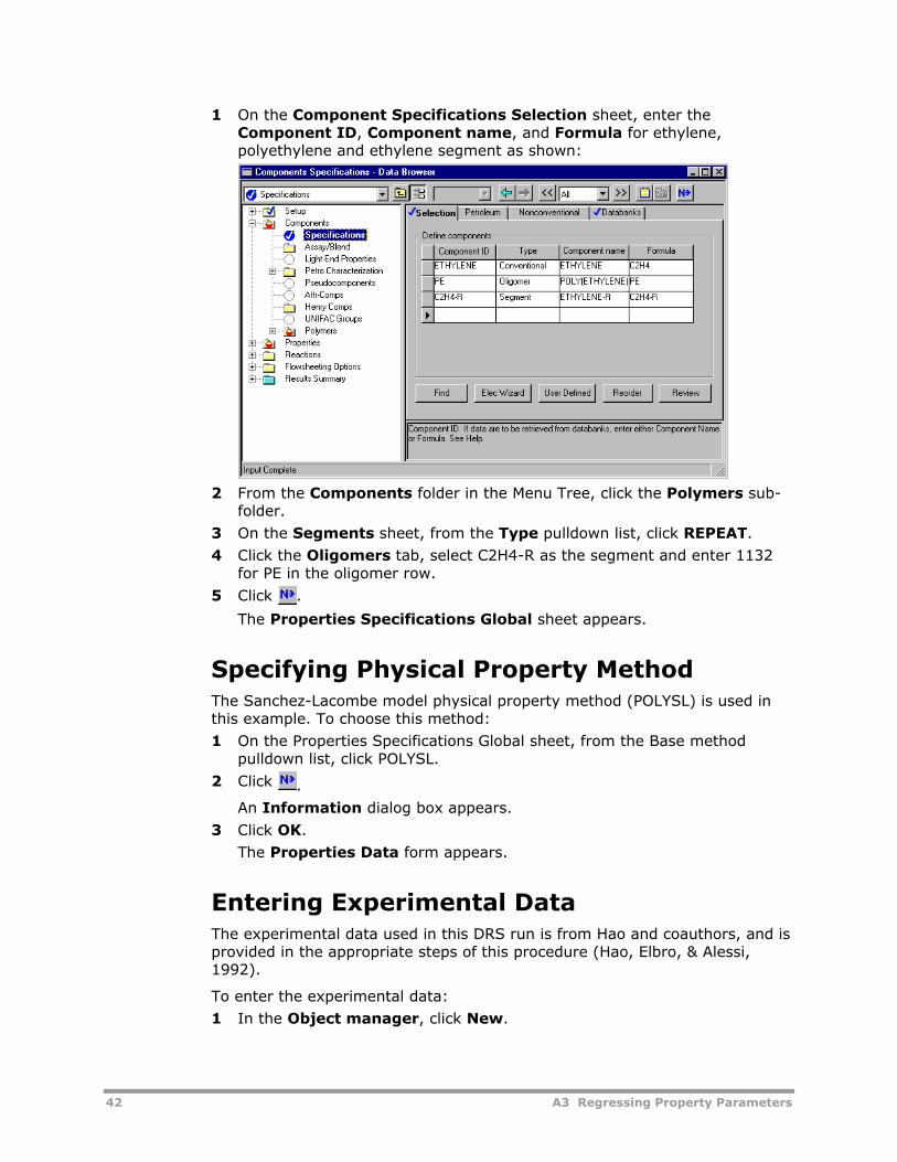
1 On the Component Specifications Selection sheet, enter the Component ID, Component name, and Formula for ethylene, polyethylene and ethylene segment as shown:
2 From the Components folder in the Menu Tree, click the Polymers sub-
folder.
3 On the Segments sheet, from the Type pulldown list, click REPEAT.
4 Click the Oligomers tab, select C2H4-R as the segment and enter 1132 for PE in the oligomer row.
5 Click .
The Properties Specifications Global sheet appears.
Specifying Physical Property Method The Sanchez-Lacombe model physical property method (POLYSL) is used in this example. To choose this method:
1 On the Properties Specifications Global sheet, from the Base method pulldown list, click POLYSL.
2 Click .
An Information dialog box appears.
3 Click OK.
The Properties Data form appears.
Entering Experimental Data The experimental data used in this DRS run is from Hao and coauthors, and is provided in the appropriate steps of this procedure (Hao, Elbro, & Alessi, 1992).
To enter the experimental data:
1 In the Object manager, click New.
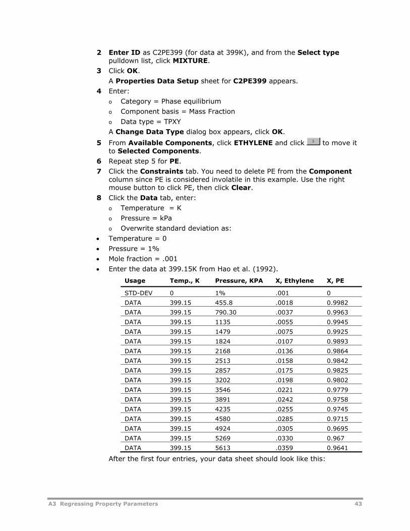
A3 Regressing Property Parameters 43
2 Enter ID as C2PE399 (for data at 399K), and from the Select type pulldown list, click MIXTURE.
3 Click OK.
A Properties Data Setup sheet for C2PE399 appears.
4 Enter:
o Category = Phase equilibrium
o Component basis = Mass Fraction
o Data type = TPXY
A Change Data Type dialog box appears, click OK.
5 From Available Components, click ETHYLENE and click to move it to Selected Components.
6 Repeat step 5 for PE.
7 Click the Constraints tab. You need to delete PE from the Component column since PE is considered involatile in this example. Use the right mouse button to click PE, then click Clear.
8 Click the Data tab, enter: o Temperature = K
o Pressure = kPa
o Overwrite standard deviation as:
• Temperature = 0
• Pressure = 1%
• Mole fraction = .001
• Enter the data at 399.15K from Hao et al. (1992).
Usage Temp., K Pressure, KPA X, Ethylene X, PE
STD-DEV 0 1% .001 0
DATA 399.15 455.8 .0018 0.9982
DATA 399.15 790.30 .0037 0.9963
DATA 399.15 1135 .0055 0.9945
DATA 399.15 1479 .0075 0.9925
DATA 399.15 1824 .0107 0.9893
DATA 399.15 2168 .0136 0.9864
DATA 399.15 2513 .0158 0.9842
DATA 399.15 2857 .0175 0.9825
DATA 399.15 3202 .0198 0.9802
DATA 399.15 3546 .0221 0.9779
DATA 399.15 3891 .0242 0.9758
DATA 399.15 4235 .0255 0.9745
DATA 399.15 4580 .0285 0.9715
DATA 399.15 4924 .0305 0.9695
DATA 399.15 5269 .0330 0.967
DATA 399.15 5613 .0359 0.9641
After the first four entries, your data sheet should look like this:
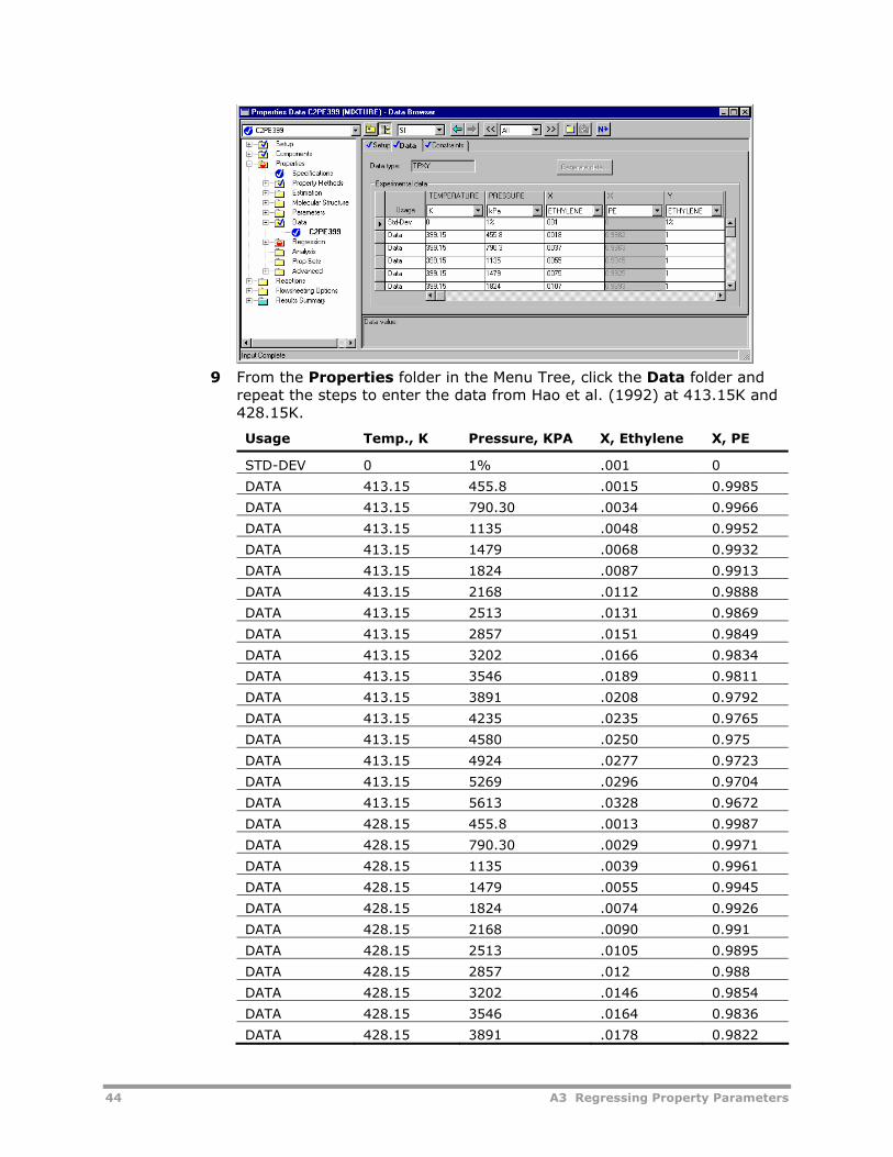
44 A3 Regressing Property Parameters
9 From the Properties folder in the Menu Tree, click the Data folder and
repeat the steps to enter the data from Hao et al. (1992) at 413.15K and 428.15K.
Usage Temp., K Pressure, KPA X, Ethylene X, PE
STD-DEV 0 1% .001 0
DATA 413.15 455.8 .0015 0.9985
DATA 413.15 790.30 .0034 0.9966
DATA 413.15 1135 .0048 0.9952
DATA 413.15 1479 .0068 0.9932
DATA 413.15 1824 .0087 0.9913
DATA 413.15 2168 .0112 0.9888
DATA 413.15 2513 .0131 0.9869
DATA 413.15 2857 .0151 0.9849
DATA 413.15 3202 .0166 0.9834
DATA 413.15 3546 .0189 0.9811
DATA 413.15 3891 .0208 0.9792
DATA 413.15 4235 .0235 0.9765
DATA 413.15 4580 .0250 0.975
DATA 413.15 4924 .0277 0.9723
DATA 413.15 5269 .0296 0.9704
DATA 413.15 5613 .0328 0.9672
DATA 428.15 455.8 .0013 0.9987
DATA 428.15 790.30 .0029 0.9971
DATA 428.15 1135 .0039 0.9961
DATA 428.15 1479 .0055 0.9945
DATA 428.15 1824 .0074 0.9926
DATA 428.15 2168 .0090 0.991
DATA 428.15 2513 .0105 0.9895
DATA 428.15 2857 .012 0.988
DATA 428.15 3202 .0146 0.9854
DATA 428.15 3546 .0164 0.9836
DATA 428.15 3891 .0178 0.9822
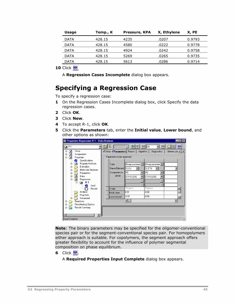
A3 Regressing Property Parameters 45
Usage Temp., K Pressure, KPA X, Ethylene X, PE
DATA 428.15 4235 .0207 0.9793
DATA 428.15 4580 .0222 0.9778
DATA 428.15 4924 .0242 0.9758
DATA 428.15 5269 .0265 0.9735
DATA 428.15 5613 .0286 0.9714
10 Click .
A Regression Cases Incomplete dialog box appears.
Specifying a Regression Case To specify a regression case:
1 On the Regression Cases Incomplete dialog box, click Specify the data regression cases.
2 Click OK.
3 Click New.
4 To accept R-1, click OK.
5 Click the Parameters tab, enter the Initial value, Lower bound, and other options as shown:
Note: The binary parameters may be specified for the oligomer-conventional species pair or for the segment-conventional species pair. For homopolymers either approach is suitable. For copolymers, the segment approach offers greater flexibility to account for the influence of polymer segmental composition on phase equilibrium.
6 Click .
A Required Properties Input Complete dialog box appears.
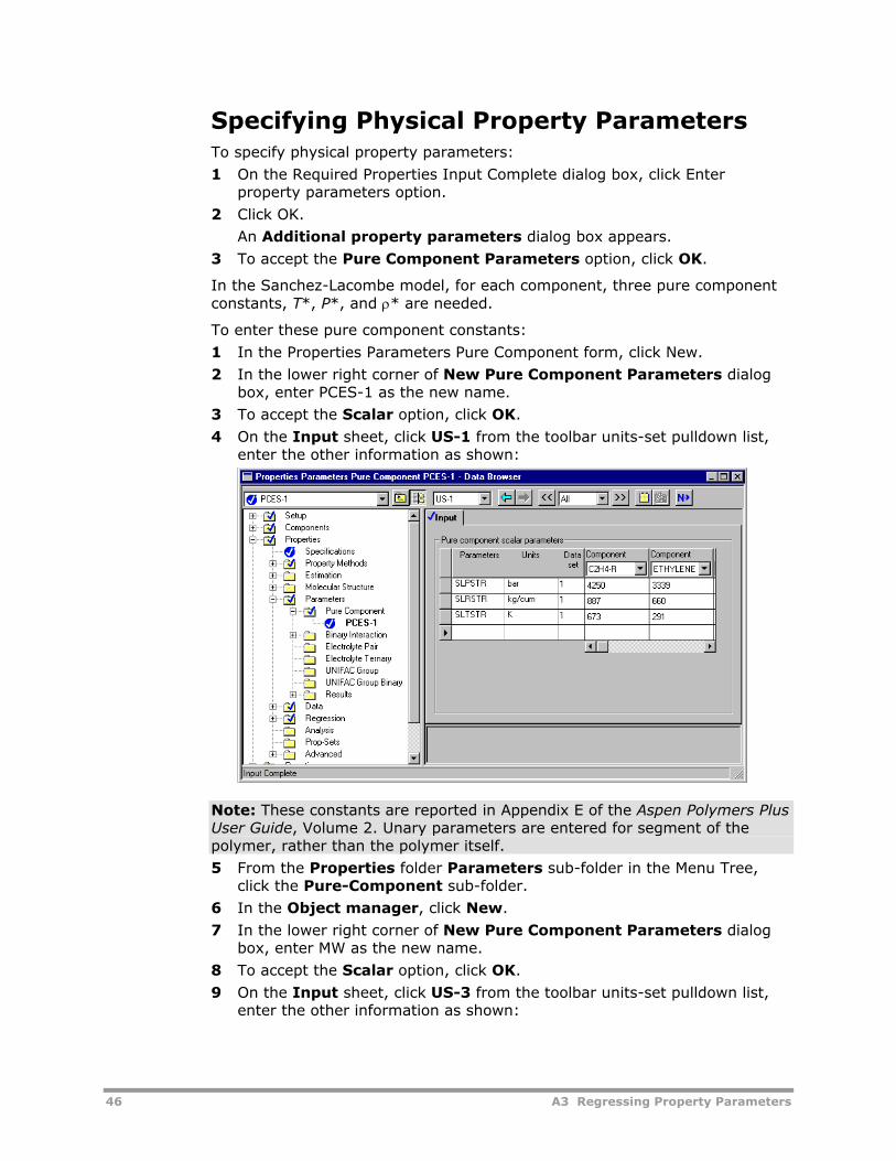
46 A3 Regressing Property Parameters
Specifying Physical Property Parameters To specify physical property parameters:
1 On the Required Properties Input Complete dialog box, click Enter property parameters option.
2 Click OK.
An Additional property parameters dialog box appears.
3 To accept the Pure Component Parameters option, click OK.
In the Sanchez-Lacombe model, for each component, three pure component constants, T*, P*, and ρ* are needed.
To enter these pure component constants:
1 In the Properties Parameters Pure Component form, click New.
2 In the lower right corner of New Pure Component Parameters dialog box, enter PCES-1 as the new name.
3 To accept the Scalar option, click OK.
4 On the Input sheet, click US-1 from the toolbar units-set pulldown list, enter the other information as shown:
Note: These constants are reported in Appendix E of the Aspen Polymers Plus User Guide, Volume 2. Unary parameters are entered for segment of the polymer, rather than the polymer itself.
5 From the Properties folder Parameters sub-folder in the Menu Tree, click the Pure-Component sub-folder.
6 In the Object manager, click New.
7 In the lower right corner of New Pure Component Parameters dialog box, enter MW as the new name.
8 To accept the Scalar option, click OK.
9 On the Input sheet, click US-3 from the toolbar units-set pulldown list, enter the other information as shown:
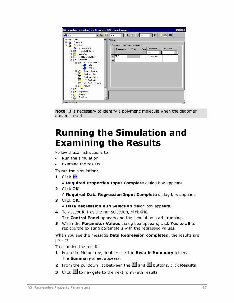
A3 Regressing Property Parameters 47
Note: It is necessary to identify a polymeric molecule when the oligomer option is used.
Running the Simulation and Examining the Results Follow these instructions to:
• Run the simulation
• Examine the results
To run the simulation:
1 Click .
A Required Properties Input Complete dialog box appears.
2 Click OK.
A Required Data Regression Input Complete dialog box appears.
3 Click OK.
A Data Regression Run Selection dialog box appears.
4 To accept R-1 as the run selection, click OK.
The Control Panel appears and the simulation starts running.
5 When the Parameter Values dialog box appears, click Yes to all to replace the existing parameters with the regressed values.
When you see the message Data Regression completed, the results are present.
To examine the results:
1 From the Menu Tree, double-click the Results Summary folder.
The Summary sheet appears.
2 From the pulldown list between the and buttons, click Results.
3 Click to navigate to the next form with results.
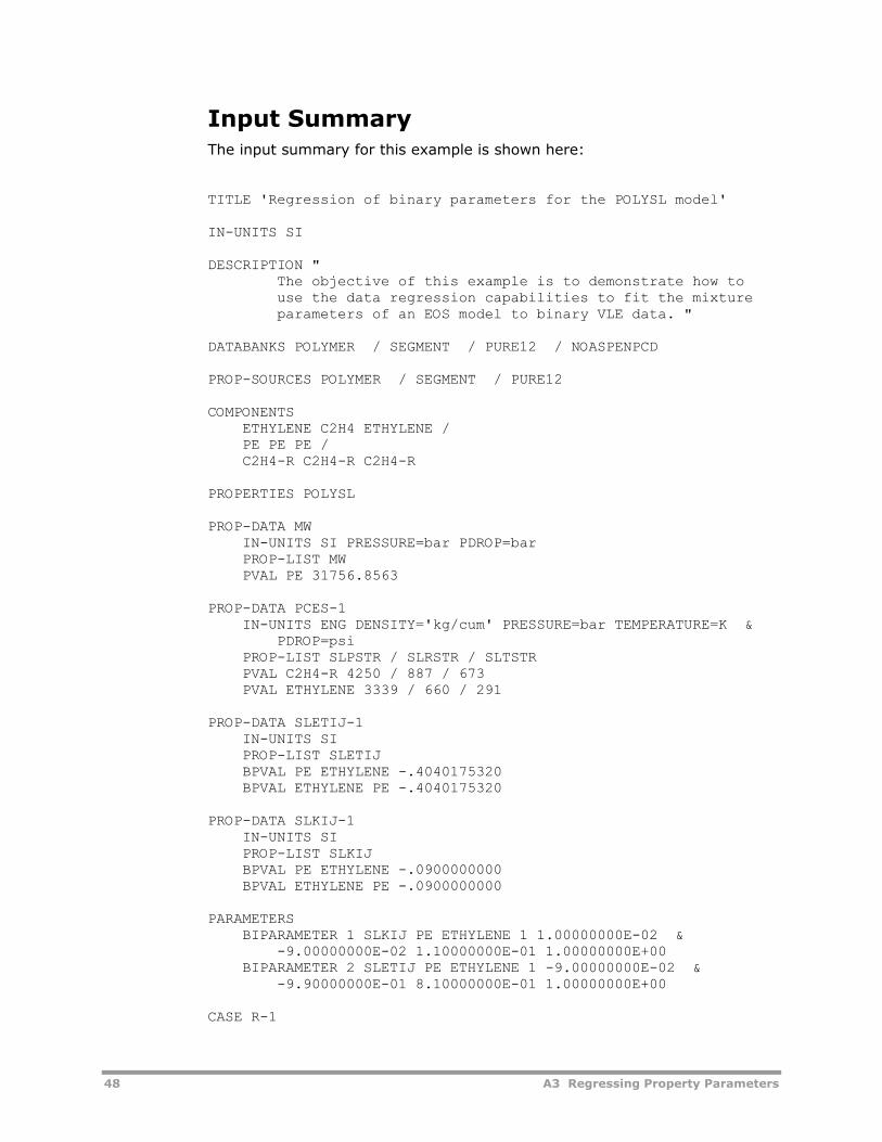
48 A3 Regressing Property Parameters
Input Summary The input summary for this example is shown here:
TITLE 'Regression of binary parameters for the POLYSL model' IN-UNITS SI DESCRIPTION " The objective of this example is to demonstrate how to use the data regression capabilities to fit the mixture parameters of an EOS model to binary VLE data. " DATABANKS POLYMER / SEGMENT / PURE12 / NOASPENPCD PROP-SOURCES POLYMER / SEGMENT / PURE12 COMPONENTS ETHYLENE C2H4 ETHYLENE / PE PE PE / C2H4-R C2H4-R C2H4-R PROPERTIES POLYSL PROP-DATA MW IN-UNITS SI PRESSURE=bar PDROP=bar PROP-LIST MW PVAL PE 31756.8563 PROP-DATA PCES-1 IN-UNITS ENG DENSITY='kg/cum' PRESSURE=bar TEMPERATURE=K & PDROP=psi PROP-LIST SLPSTR / SLRSTR / SLTSTR PVAL C2H4-R 4250 / 887 / 673 PVAL ETHYLENE 3339 / 660 / 291 PROP-DATA SLETIJ-1 IN-UNITS SI PROP-LIST SLETIJ BPVAL PE ETHYLENE -.4040175320 BPVAL ETHYLENE PE -.4040175320 PROP-DATA SLKIJ-1 IN-UNITS SI PROP-LIST SLKIJ BPVAL PE ETHYLENE -.0900000000 BPVAL ETHYLENE PE -.0900000000 PARAMETERS BIPARAMETER 1 SLKIJ PE ETHYLENE 1 1.00000000E-02 & -9.00000000E-02 1.10000000E-01 1.00000000E+00 BIPARAMETER 2 SLETIJ PE ETHYLENE 1 -9.00000000E-02 & -9.90000000E-01 8.10000000E-01 1.00000000E+00 CASE R-1
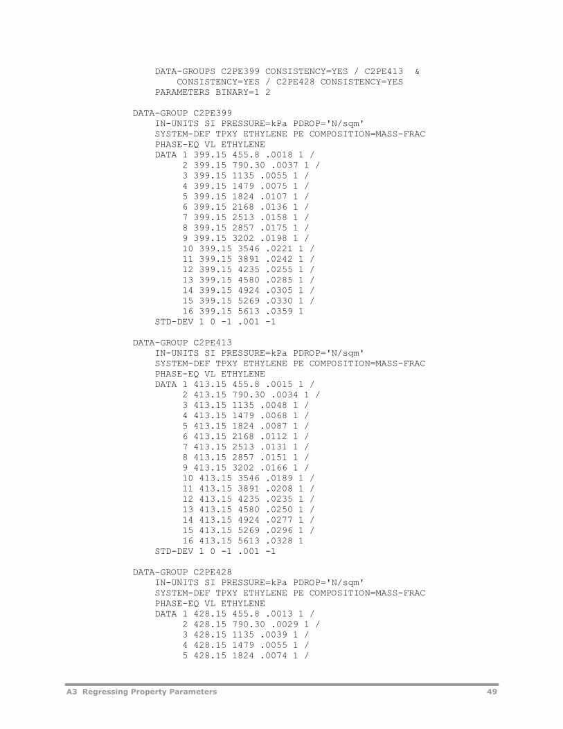
A3 Regressing Property Parameters 49
DATA-GROUPS C2PE399 CONSISTENCY=YES / C2PE413 & CONSISTENCY=YES / C2PE428 CONSISTENCY=YES PARAMETERS BINARY=1 2 DATA-GROUP C2PE399 IN-UNITS SI PRESSURE=kPa PDROP='N/sqm' SYSTEM-DEF TPXY ETHYLENE PE COMPOSITION=MASS-FRAC PHASE-EQ VL ETHYLENE DATA 1 399.15 455.8 .0018 1 / 2 399.15 790.30 .0037 1 / 3 399.15 1135 .0055 1 / 4 399.15 1479 .0075 1 / 5 399.15 1824 .0107 1 / 6 399.15 2168 .0136 1 / 7 399.15 2513 .0158 1 / 8 399.15 2857 .0175 1 / 9 399.15 3202 .0198 1 / 10 399.15 3546 .0221 1 / 11 399.15 3891 .0242 1 / 12 399.15 4235 .0255 1 / 13 399.15 4580 .0285 1 / 14 399.15 4924 .0305 1 / 15 399.15 5269 .0330 1 / 16 399.15 5613 .0359 1 STD-DEV 1 0 -1 .001 -1 DATA-GROUP C2PE413 IN-UNITS SI PRESSURE=kPa PDROP='N/sqm' SYSTEM-DEF TPXY ETHYLENE PE COMPOSITION=MASS-FRAC PHASE-EQ VL ETHYLENE DATA 1 413.15 455.8 .0015 1 / 2 413.15 790.30 .0034 1 / 3 413.15 1135 .0048 1 / 4 413.15 1479 .0068 1 / 5 413.15 1824 .0087 1 / 6 413.15 2168 .0112 1 / 7 413.15 2513 .0131 1 / 8 413.15 2857 .0151 1 / 9 413.15 3202 .0166 1 / 10 413.15 3546 .0189 1 / 11 413.15 3891 .0208 1 / 12 413.15 4235 .0235 1 / 13 413.15 4580 .0250 1 / 14 413.15 4924 .0277 1 / 15 413.15 5269 .0296 1 / 16 413.15 5613 .0328 1 STD-DEV 1 0 -1 .001 -1 DATA-GROUP C2PE428 IN-UNITS SI PRESSURE=kPa PDROP='N/sqm' SYSTEM-DEF TPXY ETHYLENE PE COMPOSITION=MASS-FRAC PHASE-EQ VL ETHYLENE DATA 1 428.15 455.8 .0013 1 / 2 428.15 790.30 .0029 1 / 3 428.15 1135 .0039 1 / 4 428.15 1479 .0055 1 / 5 428.15 1824 .0074 1 /
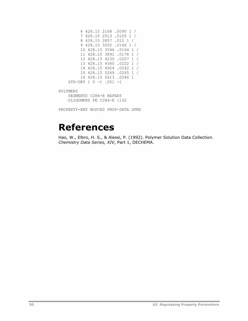
50 A3 Regressing Property Parameters
6 428.15 2168 .0090 1 / 7 428.15 2513 .0105 1 / 8 428.15 2857 .012 1 / 9 428.15 3202 .0146 1 / 10 428.15 3546 .0164 1 / 11 428.15 3891 .0178 1 / 12 428.15 4235 .0207 1 / 13 428.15 4580 .0222 1 / 14 428.15 4924 .0242 1 / 15 428.15 5269 .0265 1 / 16 428.15 5613 .0286 1 STD-DEV 1 0 -1 .001 -1 POLYMERS SEGMENTS C2H4-R REPEAT OLIGOMERS PE C2H4-R 1132 PROPERTY-REP NOPCES PROP-DATA DFMS
References Hao, W., Elbro, H. S., & Alessi, P. (1992). Polymer Solution Data Collection. Chemistry Data Series, XIV, Part 1, DECHEMA.
A4 Fitting Kinetic Parameters 51
A4 Fitting Kinetic Parameters
This example demonstrates how to fit kinetic rate constant parameters to available data for a single reactor flowsheet. This example describes the basic procedure for developing a simulation to fit kinetic parameters.
The steps covered include:
• Defining the Simulation
• Creating a New Run
• Creating the Process Flowsheet
• Specifying Setup and Global Options
• Specifying and Characterizing Components
• Specifying Physical Properties
• Specifying Polymerization Kinetics
• Supplying Process Information
• Specifying Data Regression
• Running the Simulation and Examining the Results
The Styrene Ethyl Acrylate Free-Radical Copolymerization Process application example in Section C provides strategies for fitting parameters for complex systems.
In this process, vinyl acetate is polymerized in solution in a batch reactor with methanol as a solvent and methyl peroxide as the initiator. The reactor is operated isothermally with the polymerization temperature maintained at the boiling point of methanol, 64.7°C, 1 atm.
The reactor is considered liquid filled. Therefore, vapor-liquid equilibrium calculations are not accounted for in this simulation. In practice, there is usually some vapor space in the reactor and reflux condenser. This has some effect on the concentration in the liquid phase. However, the effect is not considered significant for this homopolymerization example. The simulation can be modified to include VLE calculations if necessary.
The component information is:
Component ID Type Component Name Formula
MPO Conventional VINYL-ACETATE C4H6O2-1
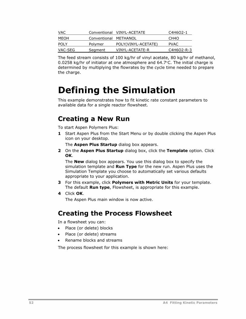
52 A4 Fitting Kinetic Parameters
VAC Conventional VINYL-ACETATE C4H6O2-1
MEOH Conventional METHANOL CH4O
POLY Polymer POLY(VINYL-ACETATE) PVAC
VAC-SEG Segment VINYL-ACETATE-R C4H6O2-R-3
The feed stream consists of 100 kg/hr of vinyl acetate, 80 kg/hr of methanol, 0.0258 kg/hr of initiator at one atmosphere and 64.7°C. The initial charge is determined by multiplying the flowrates by the cycle time needed to prepare the charge.
Defining the Simulation This example demonstrates how to fit kinetic rate constant parameters to available data for a single reactor flowsheet.
Creating a New Run To start Aspen Polymers Plus:
1 Start Aspen Plus from the Start Menu or by double clicking the Aspen Plus icon on your desktop.
The Aspen Plus Startup dialog box appears.
2 On the Aspen Plus Startup dialog box, click the Template option. Click OK.
The New dialog box appears. You use this dialog box to specify the simulation template and Run Type for the new run. Aspen Plus uses the Simulation Template you choose to automatically set various defaults appropriate to your application.
3 For this example, click Polymers with Metric Units for your template. The default Run type, Flowsheet, is appropriate for this example.
4 Click OK.
The Aspen Plus main window is now active.
Creating the Process Flowsheet In a flowsheet you can:
• Place (or delete) blocks
• Place (or delete) streams
• Rename blocks and streams
The process flowsheet for this example is shown here:
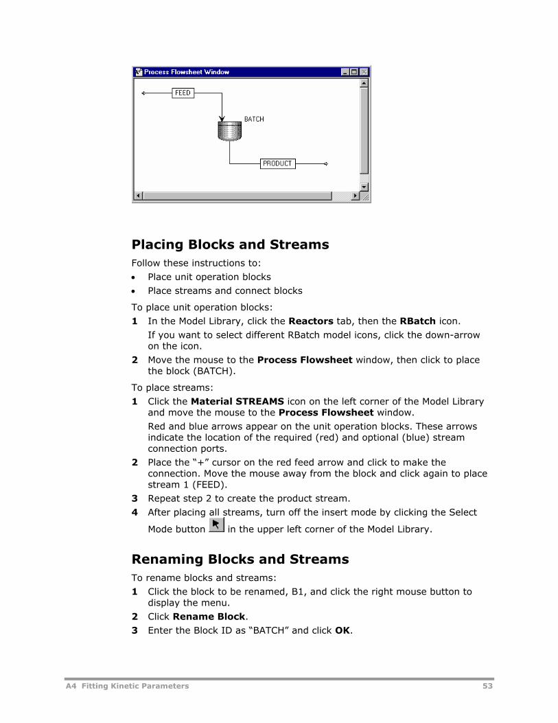
A4 Fitting Kinetic Parameters 53
Placing Blocks and Streams Follow these instructions to:
• Place unit operation blocks
• Place streams and connect blocks
To place unit operation blocks:
1 In the Model Library, click the Reactors tab, then the RBatch icon.
If you want to select different RBatch model icons, click the down-arrow on the icon.
2 Move the mouse to the Process Flowsheet window, then click to place the block (BATCH).
To place streams:
1 Click the Material STREAMS icon on the left corner of the Model Library and move the mouse to the Process Flowsheet window.
Red and blue arrows appear on the unit operation blocks. These arrows indicate the location of the required (red) and optional (blue) stream connection ports.
2 Place the “+” cursor on the red feed arrow and click to make the connection. Move the mouse away from the block and click again to place stream 1 (FEED).
3 Repeat step 2 to create the product stream.
4 After placing all streams, turn off the insert mode by clicking the Select
Mode button in the upper left corner of the Model Library.
Renaming Blocks and Streams To rename blocks and streams:
1 Click the block to be renamed, B1, and click the right mouse button to display the menu.
2 Click Rename Block.
3 Enter the Block ID as “BATCH” and click OK.
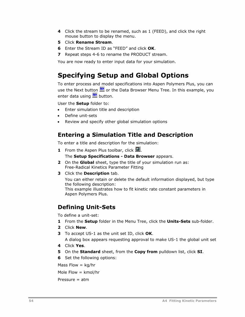
54 A4 Fitting Kinetic Parameters
4 Click the stream to be renamed, such as 1 (FEED), and click the right mouse button to display the menu.
5 Click Rename Stream.
6 Enter the Stream ID as “FEED” and click OK.
7 Repeat steps 4-6 to rename the PRODUCT stream.
You are now ready to enter input data for your simulation.
Specifying Setup and Global Options To enter process and model specifications into Aspen Polymers Plus, you can
use the Next button or the Data Browser Menu Tree. In this example, you
enter data using button.
User the Setup folder to:
• Enter simulation title and description
• Define unit-sets
• Review and specify other global simulation options
Entering a Simulation Title and Description To enter a title and description for the simulation:
1 From the Aspen Plus toolbar, click .
The Setup Specifications - Data Browser appears.
2 On the Global sheet, type the title of your simulation run as: Free-Radical Kinetics Parameter Fitting
3 Click the Description tab.
You can either retain or delete the default information displayed, but type the following description: This example illustrates how to fit kinetic rate constant parameters in Aspen Polymers Plus.
Defining Unit-Sets To define a unit-set:
1 From the Setup folder in the Menu Tree, click the Units-Sets sub-folder.
2 Click New.
3 To accept US-1 as the unit set ID, click OK.
A dialog box appears requesting approval to make US-1 the global unit set
4 Click Yes.
5 On the Standard sheet, from the Copy from pulldown list, click SI.
6 Set the following options:
Mass Flow = kg/hr
Mole Flow = kmol/hr
Pressure = atm
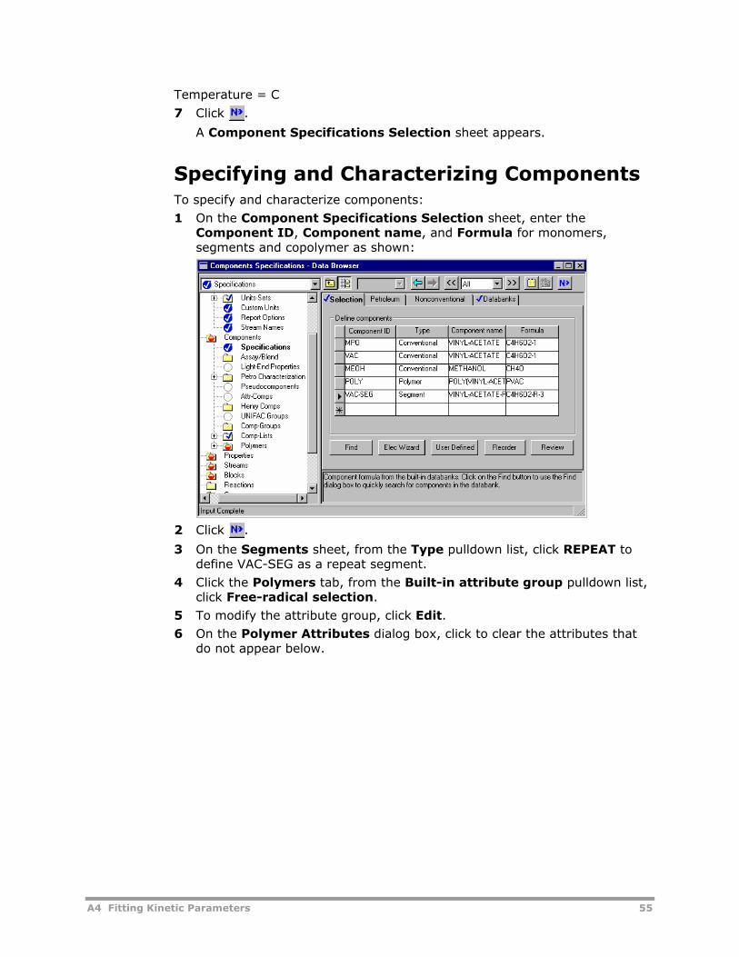
A4 Fitting Kinetic Parameters 55
Temperature = C
7 Click .
A Component Specifications Selection sheet appears.
Specifying and Characterizing Components To specify and characterize components:
1 On the Component Specifications Selection sheet, enter the Component ID, Component name, and Formula for monomers, segments and copolymer as shown:
2 Click .
3 On the Segments sheet, from the Type pulldown list, click REPEAT to define VAC-SEG as a repeat segment.
4 Click the Polymers tab, from the Built-in attribute group pulldown list, click Free-radical selection.
5 To modify the attribute group, click Edit. 6 On the Polymer Attributes dialog box, click to clear the attributes that
do not appear below.
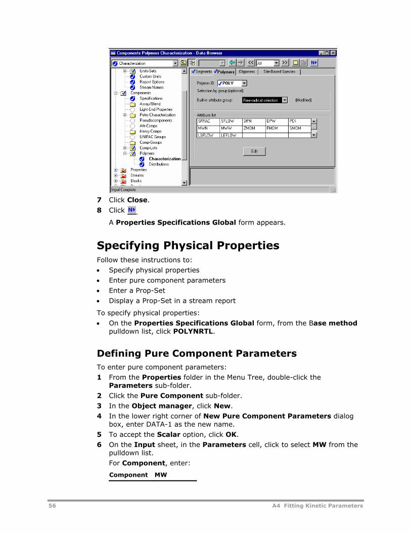
56 A4 Fitting Kinetic Parameters
7 Click Close.
8 Click .
A Properties Specifications Global form appears.
Specifying Physical Properties Follow these instructions to:
• Specify physical properties
• Enter pure component parameters
• Enter a Prop-Set
• Display a Prop-Set in a stream report
To specify physical properties:
• On the Properties Specifications Global form, from the Base method pulldown list, click POLYNRTL.
Defining Pure Component Parameters To enter pure component parameters:
1 From the Properties folder in the Menu Tree, double-click the Parameters sub-folder.
2 Click the Pure Component sub-folder.
3 In the Object manager, click New.
4 In the lower right corner of New Pure Component Parameters dialog box, enter DATA-1 as the new name.
5 To accept the Scalar option, click OK.
6 On the Input sheet, in the Parameters cell, click to select MW from the pulldown list.
For Component, enter:
Component MW
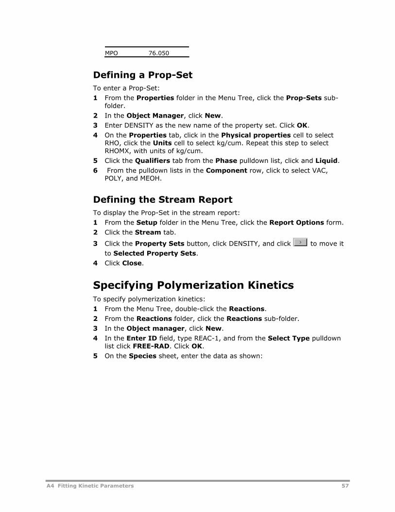
A4 Fitting Kinetic Parameters 57
MPO 76.050
Defining a Prop-Set To enter a Prop-Set:
1 From the Properties folder in the Menu Tree, click the Prop-Sets sub-folder.
2 In the Object Manager, click New.
3 Enter DENSITY as the new name of the property set. Click OK.
4 On the Properties tab, click in the Physical properties cell to select RHO, click the Units cell to select kg/cum. Repeat this step to select RHOMX, with units of kg/cum.
5 Click the Qualifiers tab from the Phase pulldown list, click and Liquid.
6 From the pulldown lists in the Component row, click to select VAC, POLY, and MEOH.
Defining the Stream Report To display the Prop-Set in the stream report:
1 From the Setup folder in the Menu Tree, click the Report Options form.
2 Click the Stream tab.
3 Click the Property Sets button, click DENSITY, and click to move it to Selected Property Sets.
4 Click Close.
Specifying Polymerization Kinetics To specify polymerization kinetics:
1 From the Menu Tree, double-click the Reactions.
2 From the Reactions folder, click the Reactions sub-folder.
3 In the Object manager, click New.
4 In the Enter ID field, type REAC-1, and from the Select Type pulldown list click FREE-RAD. Click OK.
5 On the Species sheet, enter the data as shown:
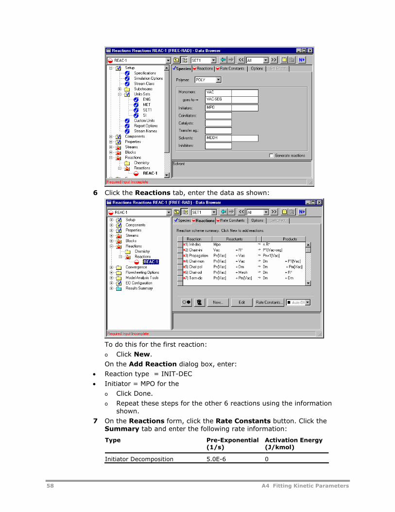
58 A4 Fitting Kinetic Parameters
6 Click the Reactions tab, enter the data as shown:
To do this for the first reaction:
o Click New.
On the Add Reaction dialog box, enter:
• Reaction type = INIT-DEC
• Initiator = MPO for the
o Click Done.
o Repeat these steps for the other 6 reactions using the information shown.
7 On the Reactions form, click the Rate Constants button. Click the Summary tab and enter the following rate information:
Type Pre-Exponential (1/s)
Activation Energy (J/kmol)
Initiator Decomposition 5.0E-6 0
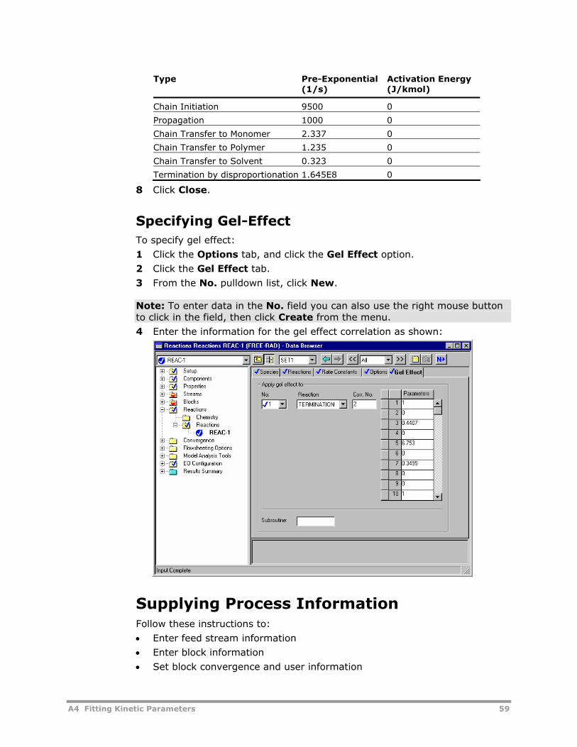
A4 Fitting Kinetic Parameters 59
Type Pre-Exponential (1/s)
Activation Energy (J/kmol)
Chain Initiation 9500 0
Propagation 1000 0
Chain Transfer to Monomer 2.337 0
Chain Transfer to Polymer 1.235 0
Chain Transfer to Solvent 0.323 0
Termination by disproportionation 1.645E8 0
8 Click Close.
Specifying Gel-Effect To specify gel effect:
1 Click the Options tab, and click the Gel Effect option.
2 Click the Gel Effect tab.
3 From the No. pulldown list, click New.
Note: To enter data in the No. field you can also use the right mouse button to click in the field, then click Create from the menu.
4 Enter the information for the gel effect correlation as shown:
Supplying Process Information Follow these instructions to:
• Enter feed stream information
• Enter block information
• Set block convergence and user information
60 A4 Fitting Kinetic Parameters
Specifying Stream Conditions To enter feed stream information:
1 From the Menu Tree, double-click the Streams folder.
2 From the Streams folder, click the FEED sub-folder.
3 On the Specifications sheet, enter the stream conditions as:
o Temperature = 64.7°C
o Pressure = 1 atm
o MPO = 0.028 kg/hr
o VAC = 100 kg/hr
o MEOH = 80 kg/hr
4 Click .
Specifying Block Conditions To enter block information:
1 On the Specifications sheet, from the Reactor operating specification pulldown list, click Constant temperature.
2 Enter:
o Temperature = 64.7°C
o Pressure = 1 atm
The Reactor field already displays Liquid-only.
3 Click the Reactions tab, click REAC-1, and click to move it to the Selected reaction sets frame.
4 Click the Stop Criteria tab, enter: o Criterion No. =1
o Location = Reactor
o Variable type = Time
o Stop value = 5
5 Click the Operation Times tab, enter:
o Total cycle time =1 hr
o Maximum calculation time = 5 hr.
o Time interval between profile points = 0.5 hr
o Maximum number of profile points = 52
Defining Block Convergence To set convergence and user information for the block:
1 From the Menu Tree Blocks folder BATCH sub-folder, click the Convergence form.
2 Click the Integration Loop tab, enter: o Integration convergence tolerance = 1E-6
o Initial step size of integration variable = 1E-7
o Maximum step size of integration variable = 0.1 hr.
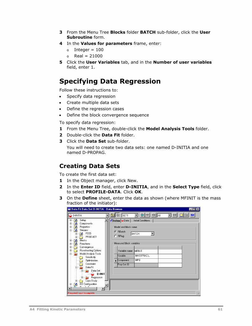
A4 Fitting Kinetic Parameters 61
3 From the Menu Tree Blocks folder BATCH sub-folder, click the User Subroutine form.
4 In the Values for parameters frame, enter:
o Integer = 100
o Real = 21000
5 Click the User Variables tab, and in the Number of user variables field, enter 1.
Specifying Data Regression Follow these instructions to:
• Specify data regression
• Create multiple data sets
• Define the regression cases
• Define the block convergence sequence
To specify data regression:
1 From the Menu Tree, double-click the Model Analysis Tools folder.
2 Double-click the Data Fit folder.
3 Click the Data Set sub-folder.
You will need to create two data sets: one named D-INITIA and one named D-PROPAG.
Creating Data Sets To create the first data set:
1 In the Object manager, click New.
2 In the Enter ID field, enter D-INITIA, and in the Select Type field, click to select PROFILE-DATA. Click OK.
3 On the Define sheet, enter the data as shown (where MFINIT is the mass fraction of the initiator):
62 A4 Fitting Kinetic Parameters
4 Click the Data tab, enter a Std-Dev of 1.0 and from the Time pulldown list, click hr.
5 Enter the time and mass fraction data as shown:
Data Point
Time (hr) Mass Fraction of Initiator
1 0.0 1.554E-4
2 0.5 1.551E-4
3 1.0 1.546E-4
4 1.5 1.542E-4
5 2.0 1.538E-4
6 2.5 1.532E-4
7 3.0 1.526E-4
8 3.5 1.522E-4
9 4.0 1.518E-4
10 4.5 1.513E-4
11 5.0 1.509E-4
6 Click the Initial Conditions tab, enter:
o Temperature = 65°C
o Pressure = 1 atm
The Reactor type and Block name fields already display RBATCH and BATCH respectively.
To create the second data set:
1 From the Menu Tree Model Analysis Tools folder Data Fit sub-folder, click the Data Set sub-folder.
2 In the Object manager, click New.
3 In the Enter ID field, enter D-PROPAG, and in the Select Type field, click to select PROFILE-DATA. Click OK.
4 On the Define sheet, enter: o Variable name = DUTY
o Variable = DUTY
o Model and block name = BATCH
RBATCH is already selected as the Block name.
5 Click the Data tab, enter a Std-Dev of 5.0.
Enter the time and heat release data shown:
Data Point
Time (hr) Instantaneous Heat Release (Watt)
2 0.5 -3750.0
3 1.0 -3700.0
4 1.5 -3300.0
5 2.0 -3250.0
6 2.5 -3100.0
7 3.0 -3000.0
8 3.5 -2800.0
9 4.0 -2650.0
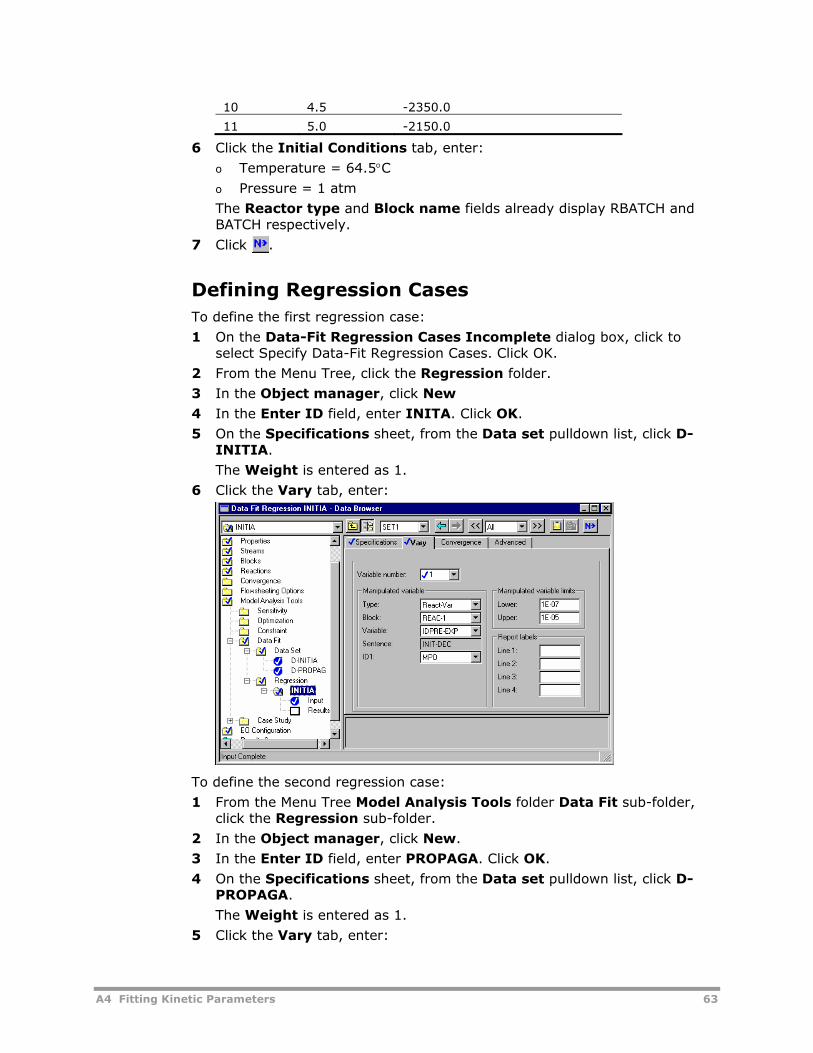
A4 Fitting Kinetic Parameters 63
10 4.5 -2350.0
11 5.0 -2150.0
6 Click the Initial Conditions tab, enter:
o Temperature = 64.5°C
o Pressure = 1 atm
The Reactor type and Block name fields already display RBATCH and BATCH respectively.
7 Click .
Defining Regression Cases To define the first regression case:
1 On the Data-Fit Regression Cases Incomplete dialog box, click to select Specify Data-Fit Regression Cases. Click OK.
2 From the Menu Tree, click the Regression folder.
3 In the Object manager, click New
4 In the Enter ID field, enter INITA. Click OK.
5 On the Specifications sheet, from the Data set pulldown list, click D-INITIA.
The Weight is entered as 1.
6 Click the Vary tab, enter:
To define the second regression case:
1 From the Menu Tree Model Analysis Tools folder Data Fit sub-folder, click the Regression sub-folder.
2 In the Object manager, click New.
3 In the Enter ID field, enter PROPAGA. Click OK.
4 On the Specifications sheet, from the Data set pulldown list, click D-PROPAGA.
The Weight is entered as 1.
5 Click the Vary tab, enter:
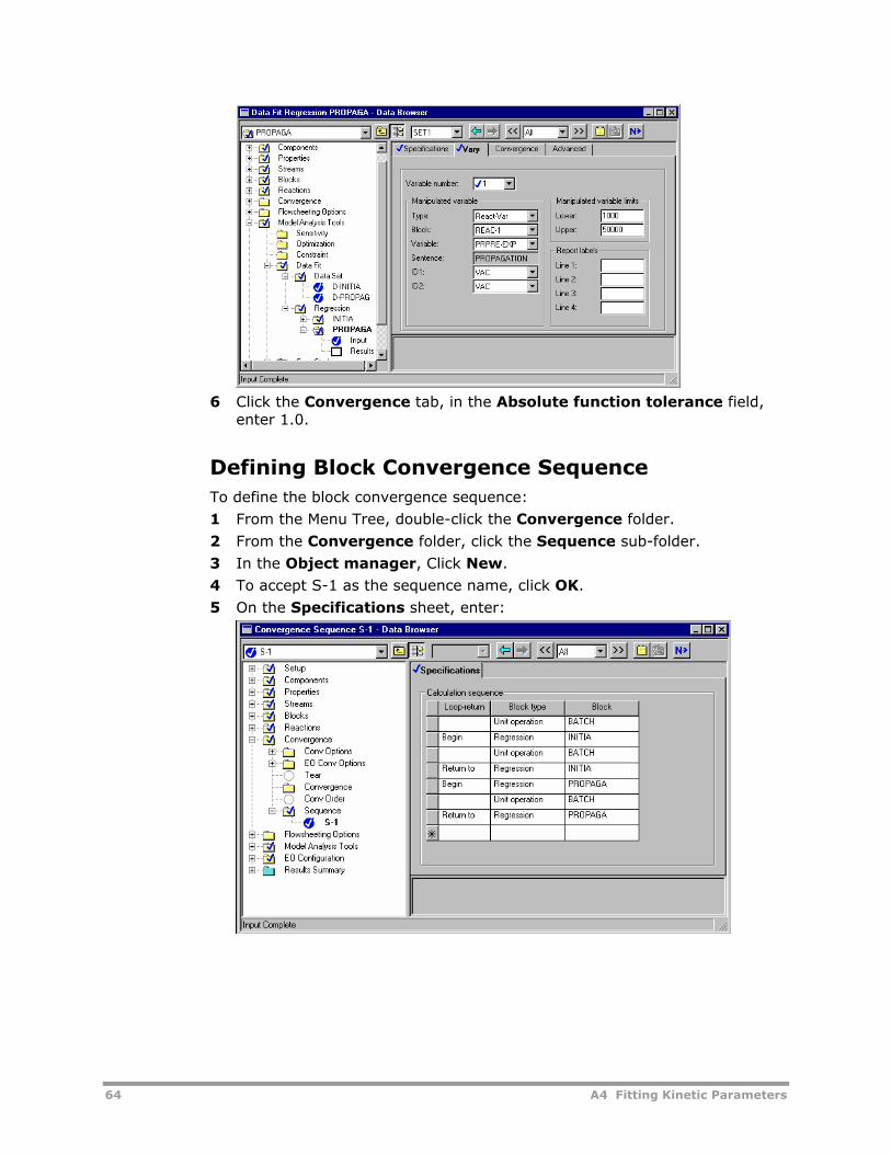
64 A4 Fitting Kinetic Parameters
6 Click the Convergence tab, in the Absolute function tolerance field,
enter 1.0.
Defining Block Convergence Sequence To define the block convergence sequence:
1 From the Menu Tree, double-click the Convergence folder.
2 From the Convergence folder, click the Sequence sub-folder.
3 In the Object manager, Click New.
4 To accept S-1 as the sequence name, click OK.
5 On the Specifications sheet, enter:
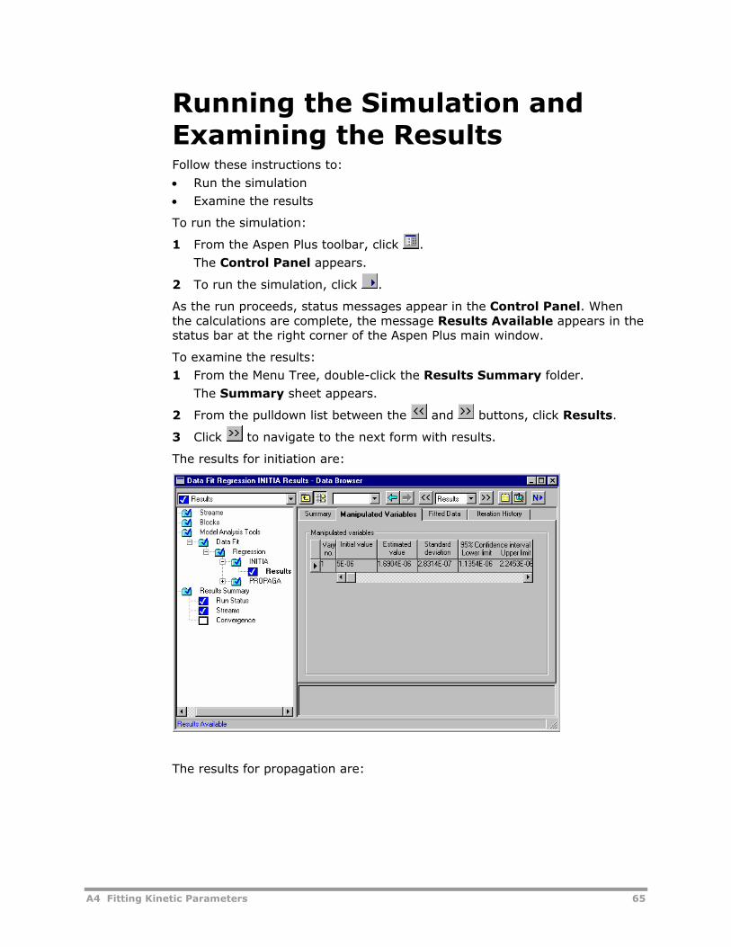
A4 Fitting Kinetic Parameters 65
Running the Simulation and Examining the Results Follow these instructions to:
• Run the simulation
• Examine the results
To run the simulation:
1 From the Aspen Plus toolbar, click .
The Control Panel appears.
2 To run the simulation, click .
As the run proceeds, status messages appear in the Control Panel. When the calculations are complete, the message Results Available appears in the status bar at the right corner of the Aspen Plus main window.
To examine the results:
1 From the Menu Tree, double-click the Results Summary folder.
The Summary sheet appears.
2 From the pulldown list between the and buttons, click Results.
3 Click to navigate to the next form with results.
The results for initiation are:
The results for propagation are:
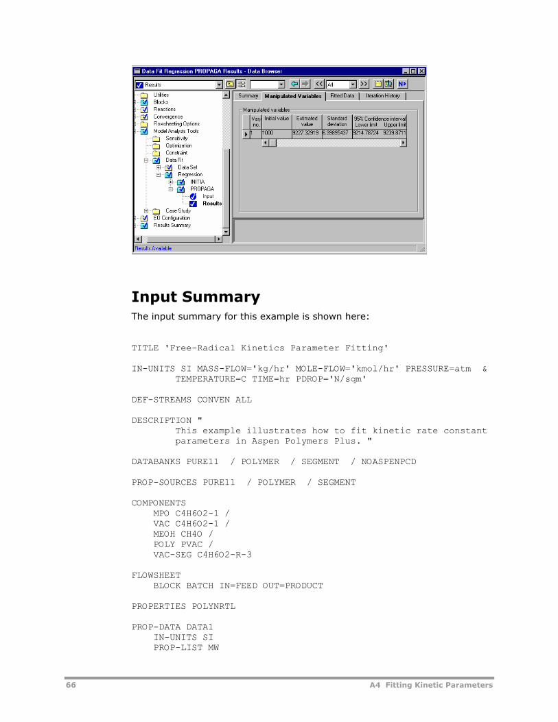
66 A4 Fitting Kinetic Parameters
Input Summary The input summary for this example is shown here:
TITLE 'Free-Radical Kinetics Parameter Fitting' IN-UNITS SI MASS-FLOW='kg/hr' MOLE-FLOW='kmol/hr' PRESSURE=atm & TEMPERATURE=C TIME=hr PDROP='N/sqm' DEF-STREAMS CONVEN ALL DESCRIPTION " This example illustrates how to fit kinetic rate constant parameters in Aspen Polymers Plus. " DATABANKS PURE11 / POLYMER / SEGMENT / NOASPENPCD PROP-SOURCES PURE11 / POLYMER / SEGMENT COMPONENTS MPO C4H6O2-1 / VAC C4H6O2-1 / MEOH CH4O / POLY PVAC / VAC-SEG C4H6O2-R-3 FLOWSHEET BLOCK BATCH IN=FEED OUT=PRODUCT PROPERTIES POLYNRTL PROP-DATA DATA1 IN-UNITS SI PROP-LIST MW
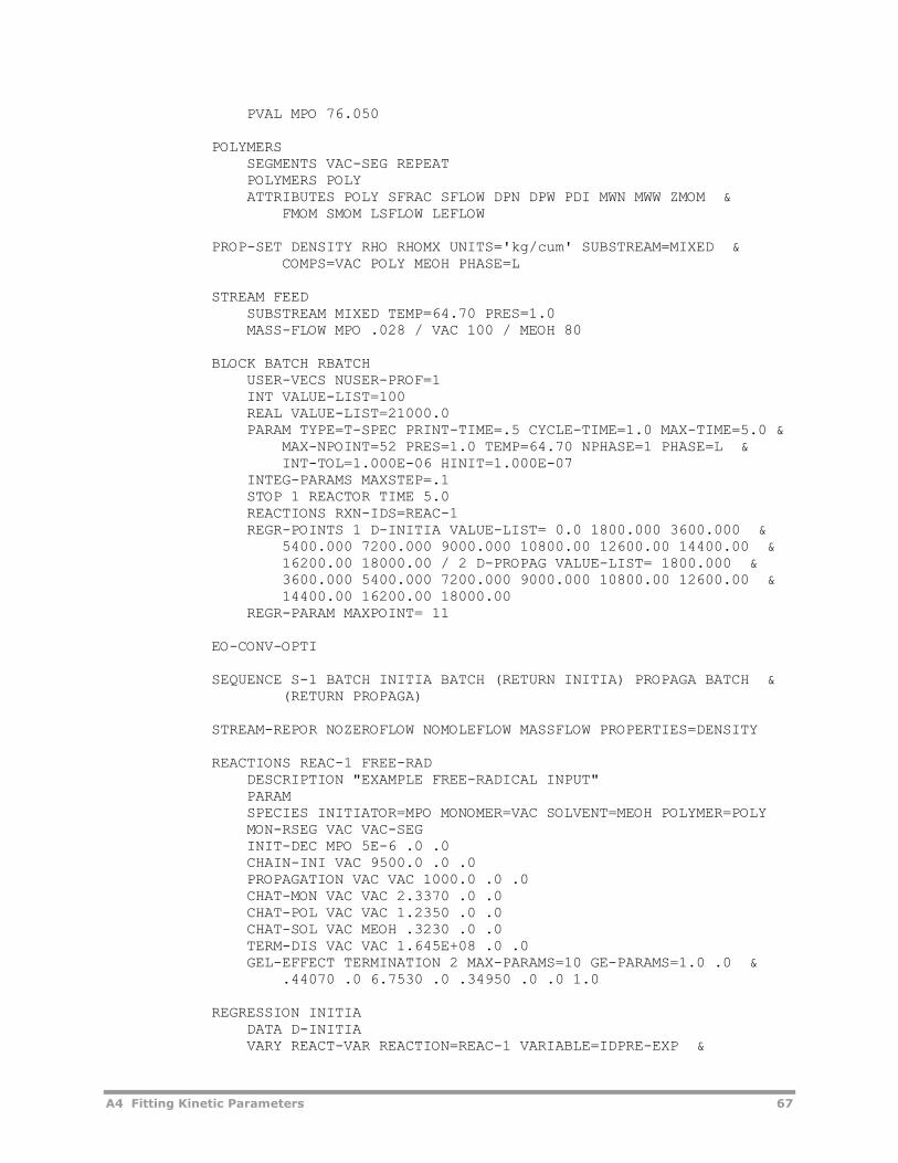
A4 Fitting Kinetic Parameters 67
PVAL MPO 76.050 POLYMERS SEGMENTS VAC-SEG REPEAT POLYMERS POLY ATTRIBUTES POLY SFRAC SFLOW DPN DPW PDI MWN MWW ZMOM & FMOM SMOM LSFLOW LEFLOW PROP-SET DENSITY RHO RHOMX UNITS='kg/cum' SUBSTREAM=MIXED & COMPS=VAC POLY MEOH PHASE=L STREAM FEED SUBSTREAM MIXED TEMP=64.70 PRES=1.0 MASS-FLOW MPO .028 / VAC 100 / MEOH 80 BLOCK BATCH RBATCH USER-VECS NUSER-PROF=1 INT VALUE-LIST=100 REAL VALUE-LIST=21000.0 PARAM TYPE=T-SPEC PRINT-TIME=.5 CYCLE-TIME=1.0 MAX-TIME=5.0 & MAX-NPOINT=52 PRES=1.0 TEMP=64.70 NPHASE=1 PHASE=L & INT-TOL=1.000E-06 HINIT=1.000E-07 INTEG-PARAMS MAXSTEP=.1 STOP 1 REACTOR TIME 5.0 REACTIONS RXN-IDS=REAC-1 REGR-POINTS 1 D-INITIA VALUE-LIST= 0.0 1800.000 3600.000 & 5400.000 7200.000 9000.000 10800.00 12600.00 14400.00 & 16200.00 18000.00 / 2 D-PROPAG VALUE-LIST= 1800.000 & 3600.000 5400.000 7200.000 9000.000 10800.00 12600.00 & 14400.00 16200.00 18000.00 REGR-PARAM MAXPOINT= 11 EO-CONV-OPTI SEQUENCE S-1 BATCH INITIA BATCH (RETURN INITIA) PROPAGA BATCH & (RETURN PROPAGA) STREAM-REPOR NOZEROFLOW NOMOLEFLOW MASSFLOW PROPERTIES=DENSITY REACTIONS REAC-1 FREE-RAD DESCRIPTION "EXAMPLE FREE-RADICAL INPUT" PARAM SPECIES INITIATOR=MPO MONOMER=VAC SOLVENT=MEOH POLYMER=POLY MON-RSEG VAC VAC-SEG INIT-DEC MPO 5E-6 .0 .0 CHAIN-INI VAC 9500.0 .0 .0 PROPAGATION VAC VAC 1000.0 .0 .0 CHAT-MON VAC VAC 2.3370 .0 .0 CHAT-POL VAC VAC 1.2350 .0 .0 CHAT-SOL VAC MEOH .3230 .0 .0 TERM-DIS VAC VAC 1.645E+08 .0 .0 GEL-EFFECT TERMINATION 2 MAX-PARAMS=10 GE-PARAMS=1.0 .0 & .44070 .0 6.7530 .0 .34950 .0 .0 1.0 REGRESSION INITIA DATA D-INITIA VARY REACT-VAR REACTION=REAC-1 VARIABLE=IDPRE-EXP &
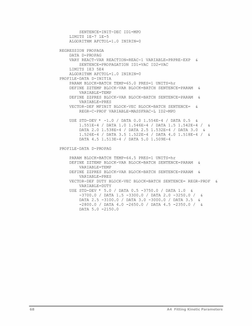
68 A4 Fitting Kinetic Parameters
SENTENCE=INIT-DEC ID1=MPO LIMITS 1E-7 1E-5 ALGORITHM AFCTOL=1.0 INIRIN=0 REGRESSION PROPAGA DATA D-PROPAG VARY REACT-VAR REACTION=REAC-1 VARIABLE=PRPRE-EXP & SENTENCE=PROPAGATION ID1=VAC ID2=VAC LIMITS 1E3 5E4 ALGORITHM AFCTOL=1.0 INIRIN=0 PROFILE-DATA D-INITIA PARAM BLOCK=BATCH TEMP=65.0 PRES=1 UNITS=hr DEFINE ZZTEMP BLOCK-VAR BLOCK=BATCH SENTENCE=PARAM & VARIABLE=TEMP DEFINE ZZPRES BLOCK-VAR BLOCK=BATCH SENTENCE=PARAM & VARIABLE=PRES VECTOR-DEF MFINIT BLOCK-VEC BLOCK=BATCH SENTENCE= & REGR-C-PROF VARIABLE=MASSFRAC-L ID2=MPO USE STD-DEV * -1.0 / DATA 0.0 1.554E-4 / DATA 0.5 & 1.551E-4 / DATA 1.0 1.546E-4 / DATA 1.5 1.542E-4 / & DATA 2.0 1.538E-4 / DATA 2.5 1.532E-4 / DATA 3.0 & 1.526E-4 / DATA 3.5 1.522E-4 / DATA 4.0 1.518E-4 / & DATA 4.5 1.513E-4 / DATA 5.0 1.509E-4 PROFILE-DATA D-PROPAG PARAM BLOCK=BATCH TEMP=64.5 PRES=1 UNITS=hr DEFINE ZZTEMP BLOCK-VAR BLOCK=BATCH SENTENCE=PARAM & VARIABLE=TEMP DEFINE ZZPRES BLOCK-VAR BLOCK=BATCH SENTENCE=PARAM & VARIABLE=PRES VECTOR-DEF DUTY BLOCK-VEC BLOCK=BATCH SENTENCE= REGR-PROF & VARIABLE=DUTY USE STD-DEV * 5.0 / DATA 0.5 -3750.0 / DATA 1.0 & -3700.0 / DATA 1.5 -3300.0 / DATA 2.0 -3250.0 / & DATA 2.5 -3100.0 / DATA 3.0 -3000.0 / DATA 3.5 & -2800.0 / DATA 4.0 -2650.0 / DATA 4.5 -2350.0 / & DATA 5.0 -2150.0
A5 Fractionating Oligomers 69
A5 Fractionating Oligomers
This example illustrates the use of Aspen Polymers Plus for modeling a polymer/oligomer fractionation process.
The steps covered include:
• Defining the Simulation
• Creating a New Run
• Creating the Process Flowsheet
• Specifying Setup and Global Options
• Specifying and Characterizing Components
• Specifying Physical Properties
• Supplying Process Information
• Running the Simulation and Examining the Results
One typical fractionation method is to dissolve the polymer in a good solvent and then add small amounts of antisolvent to it. At the phase equilibria, the high-molecular weight polymer precipitates in the solvent phase, while the lower-molecular weight polymer dissolves in the antisolvent phase. By continuing addition of antisolvent, progressively lower molecular-weight polymer precipitates.
The system in this example contains benzene (1, solvent), ethanol (2, antisolvent) and polystyrene (3, polymer). A pseudo-component approach is used to represent the polydispersity of polystyrene. In the pseudo-component approach, a series of oligomers with different degree of polymerization (DP) is defined. The mass distribution of the oligomers in the feed is approximately a Gamma distribution. The Flory-Huggins model of polymer solution is used to calculate the liquid-liquid phase equilibria in this quasi-ternary mixture. The Flory-Huggins binary interaction parameters χ are obtained from Wu and Prausnitz (Wu & Prausnitz, 1990).
Defining the Simulation In this example you create an Aspen Polymers Plus process model to fractionate polystyrene using benzene and ethanol, run the simulation, and examine the results.
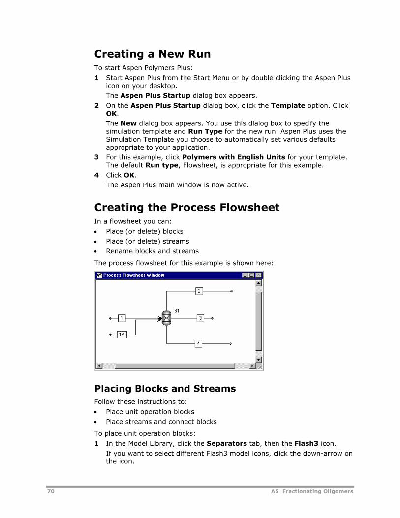
70 A5 Fractionating Oligomers
Creating a New Run To start Aspen Polymers Plus:
1 Start Aspen Plus from the Start Menu or by double clicking the Aspen Plus icon on your desktop.
The Aspen Plus Startup dialog box appears.
2 On the Aspen Plus Startup dialog box, click the Template option. Click OK.
The New dialog box appears. You use this dialog box to specify the simulation template and Run Type for the new run. Aspen Plus uses the Simulation Template you choose to automatically set various defaults appropriate to your application.
3 For this example, click Polymers with English Units for your template. The default Run type, Flowsheet, is appropriate for this example.
4 Click OK.
The Aspen Plus main window is now active.
Creating the Process Flowsheet In a flowsheet you can:
• Place (or delete) blocks
• Place (or delete) streams
• Rename blocks and streams
The process flowsheet for this example is shown here:
Placing Blocks and Streams Follow these instructions to:
• Place unit operation blocks
• Place streams and connect blocks
To place unit operation blocks:
1 In the Model Library, click the Separators tab, then the Flash3 icon.
If you want to select different Flash3 model icons, click the down-arrow on the icon.
A5 Fractionating Oligomers 71
2 Move the mouse to the Process Flowsheet window, then click to place the block (B1).
To place streams:
1 Click the Material STREAMS icon on the left corner of the Model Library and move the mouse to the Process Flowsheet window.
Red and blue arrows appear on the unit operation blocks. These arrows indicate the location of the required (red) and optional (blue) stream connection ports.
2 Place the “+” cursor on the red feed arrow and click to make the connection. Move the mouse away from the block and click again to place stream 1.
3 Repeat step 2 to create the other streams.
4 After placing all streams, turn off the insert mode by clicking the Select
Mode button in the upper left corner of the Model Library.
Renaming Streams To rename streams:
1 Click the stream to be renamed, such as 5, and click the right mouse button to display the menu.
2 Click Rename Stream.
3 Enter the Stream ID as “1P” and click OK.
You are now ready to enter input data for your simulation.
Specifying Setup and Global Options To enter process and model specifications into Aspen Polymers Plus, you can
use the Next button or the Data Browser Menu Tree. In this example, you enter data using the Menu Tree.
Use the Setup folder to:
• Enter a simulation title
• Define unit-sets
• Specify report options
Entering a Simulation Title and Description To enter a title and description for the simulation:
1 From the Data menu, click Setup.
The Setup Specifications - Data Browser appears.
2 On the Global sheet, type the title of your simulation run as: Polystyrene Oligomer Fractionation
3 Click the Description tab.
You can either retain or delete the default information displayed, but type the following description:
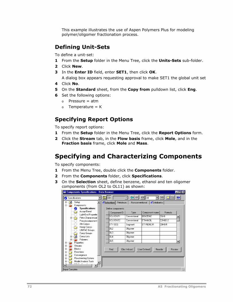
72 A5 Fractionating Oligomers
This example illustrates the use of Aspen Polymers Plus for modeling polymer/oligomer fractionation process.
Defining Unit-Sets To define a unit-set:
1 From the Setup folder in the Menu Tree, click the Units-Sets sub-folder.
2 Click New.
3 In the Enter ID field, enter SET1, then click OK.
A dialog box appears requesting approval to make SET1 the global unit set
4 Click No.
5 On the Standard sheet, from the Copy from pulldown list, click Eng.
6 Set the following options:
o Pressure = atm
o Temperature = K
Specifying Report Options To specify report options:
1 From the Setup folder in the Menu Tree, click the Report Options form.
2 Click the Stream tab, in the Flow basis frame, click Mole, and in the Fraction basis frame, click Mole and Mass.
Specifying and Characterizing Components To specify components:
1 From the Menu Tree, double click the Components folder.
2 From the Components folder, click Specifications.
3 On the Selection sheet, define benzene, ethanol and ten oligomer components (from OL2 to OL11) as shown:
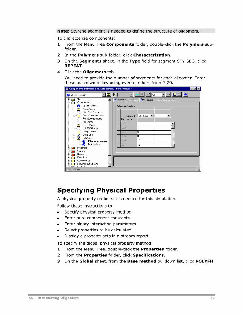
A5 Fractionating Oligomers 73
Note: Styrene segment is needed to define the structure of oligomers.
To characterize components:
1 From the Menu Tree Components folder, double-click the Polymers sub-folder.
2 In the Polymers sub-folder, click Characterization.
3 On the Segments sheet, in the Type field for segment STY-SEG, click REPEAT.
4 Click the Oligomers tab.
You need to provide the number of segments for each oligomer. Enter these as shown below using even numbers from 2-20.
Specifying Physical Properties A physical property option set is needed for this simulation.
Follow these instructions to:
• Specify physical property method
• Enter pure component constants
• Enter binary interaction parameters
• Select properties to be calculated
• Display a property sets in a stream report
To specify the global physical property method:
1 From the Menu Tree, double-click the Properties folder.
2 From the Properties folder, click Specifications.
3 On the Global sheet, from the Base method pulldown list, click POLYFH.
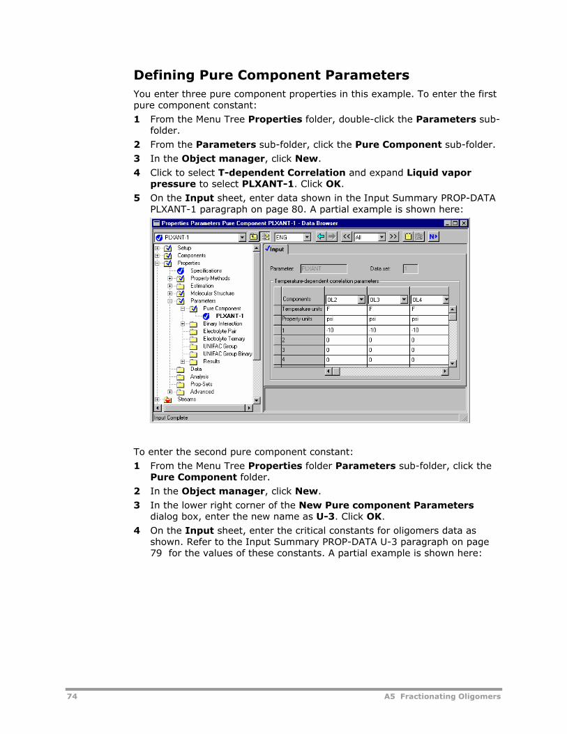
74 A5 Fractionating Oligomers
Defining Pure Component Parameters You enter three pure component properties in this example. To enter the first pure component constant:
1 From the Menu Tree Properties folder, double-click the Parameters sub-folder.
2 From the Parameters sub-folder, click the Pure Component sub-folder.
3 In the Object manager, click New.
4 Click to select T-dependent Correlation and expand Liquid vapor pressure to select PLXANT-1. Click OK.
5 On the Input sheet, enter data shown in the Input Summary PROP-DATA PLXANT-1 paragraph on page 80. A partial example is shown here:
To enter the second pure component constant:
1 From the Menu Tree Properties folder Parameters sub-folder, click the Pure Component folder.
2 In the Object manager, click New.
3 In the lower right corner of the New Pure component Parameters dialog box, enter the new name as U-3. Click OK.
4 On the Input sheet, enter the critical constants for oligomers data as shown. Refer to the Input Summary PROP-DATA U-3 paragraph on page 79 for the values of these constants. A partial example is shown here:
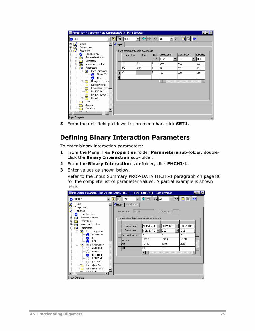
A5 Fractionating Oligomers 75
5 From the unit field pulldown list on menu bar, click SET1.
Defining Binary Interaction Parameters To enter binary interaction parameters:
1 From the Menu Tree Properties folder Parameters sub-folder, double-click the Binary Interaction sub-folder.
2 From the Binary Interaction sub-folder, click FHCHI-1.
3 Enter values as shown below.
Refer to the Input Summary PROP-DATA FHCHI-1 paragraph on page 80 for the complete list of parameter values. A partial example is shown here:
76 A5 Fractionating Oligomers
Defining Properties to be Calculated To select the properties to be calculated:
1 From the Menu Tree Properties folder, click the Prop-Sets sub-folder.
2 In the Object manager, click New.
3 To accept PS-1 as the new name, Click OK.
4 On the Properties sheet, in the Physical properties field, click GAMMA.
5 Click the Qualifiers tab, from the Phase pulldown list, click Liquid.
Defining the Stream Report To display the property set in the stream report:
1 From the Setup folder in the Menu Tree, click the Report Options form.
2 Click the Stream tab, and click the Property Sets button.
3 Click PS-1, then click to move it to the Selected property sets frame. Click Close.
Supplying Process Information Follow these instructions to specify:
• Stream conditions
• Block specifications
Specifying Stream Conditions To specify the stream condition for the oligomer and non-solvent streams:
1 From the Menu Tree, double-click the Streams folder.
2 From the Streams folder, click the 1 folder.
3 On the Specifications sheet, enter the mass flow and feed condition as follows:
o Temperature = 101.5 F
o Pressure = 14.7 psi
o Total flow (Mass) = 2.1 lb/hr
o Solvent 2 = 2.1 lb/hr
4 From Streams folder in the Menu Tree, click the 1P sub-folder.
5 On the Specifications sheet, enter the data as shown:
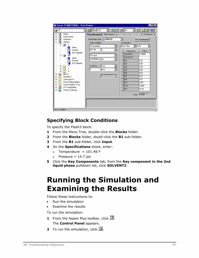
A5 Fractionating Oligomers 77
Specifying Block Conditions To specify the Flash3 block:
1 From the Menu Tree, double-click the Blocks folder.
2 From the Blocks folder, doubl-click the B1 sub-folder.
3 From the B1 sub-folder, click Input.
4 On the Specifications sheet, enter:
o Temperature = 101.48 F
o Pressure = 14.7 psi
5 Click the Key Components tab, from the Key component in the 2nd liquid phase pulldown list, click SOLVENT2.
Running the Simulation and Examining the Results Follow these instructions to:
• Run the simulation
• Examine the results
To run the simulation:
1 From the Aspen Plus toolbar, click .
The Control Panel appears.
2 To run the simulation, click .
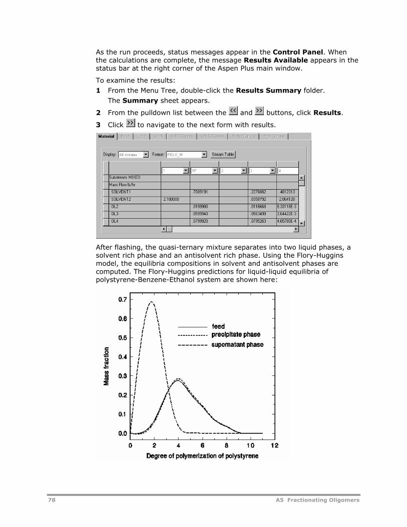
78 A5 Fractionating Oligomers
As the run proceeds, status messages appear in the Control Panel. When the calculations are complete, the message Results Available appears in the status bar at the right corner of the Aspen Plus main window.
To examine the results:
1 From the Menu Tree, double-click the Results Summary folder.
The Summary sheet appears.
2 From the pulldown list between the and buttons, click Results.
3 Click to navigate to the next form with results.
After flashing, the quasi-ternary mixture separates into two liquid phases, a solvent rich phase and an antisolvent rich phase. Using the Flory-Huggins model, the equilibria compositions in solvent and antisolvent phases are computed. The Flory-Huggins predictions for liquid-liquid equilibria of polystyrene-Benzene-Ethanol system are shown here:
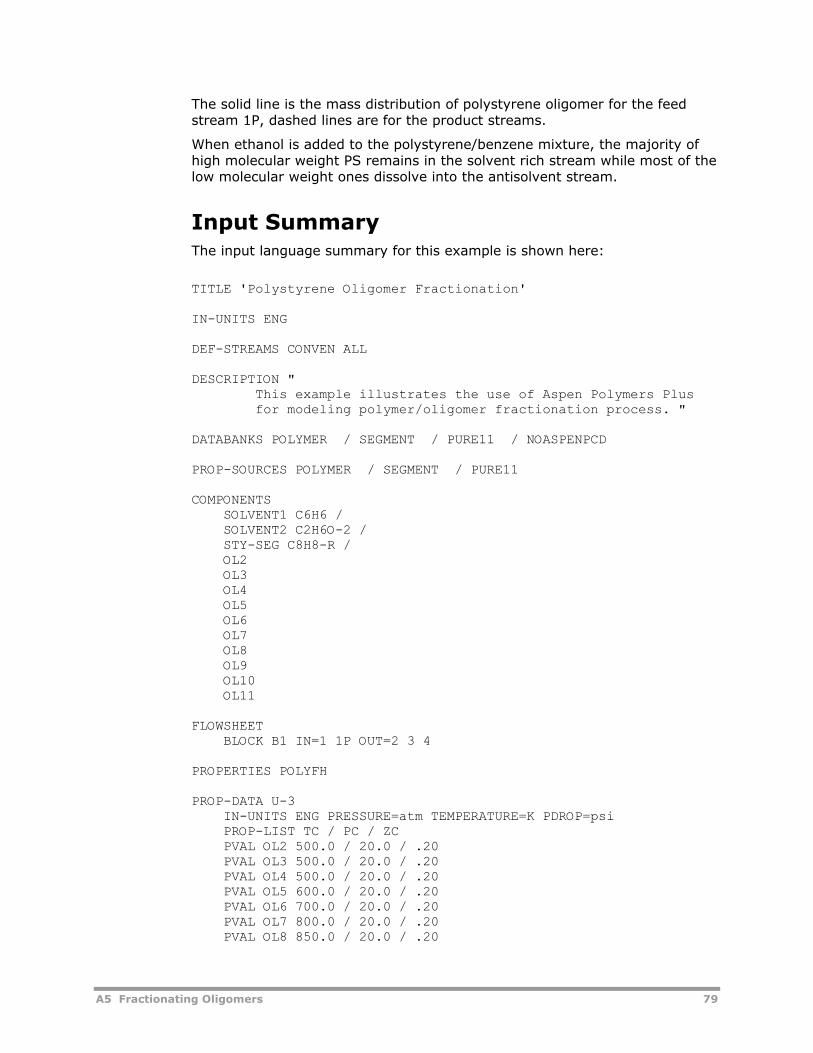
A5 Fractionating Oligomers 79
The solid line is the mass distribution of polystyrene oligomer for the feed stream 1P, dashed lines are for the product streams.
When ethanol is added to the polystyrene/benzene mixture, the majority of high molecular weight PS remains in the solvent rich stream while most of the low molecular weight ones dissolve into the antisolvent stream.
Input Summary The input language summary for this example is shown here:
TITLE 'Polystyrene Oligomer Fractionation' IN-UNITS ENG DEF-STREAMS CONVEN ALL DESCRIPTION " This example illustrates the use of Aspen Polymers Plus for modeling polymer/oligomer fractionation process. " DATABANKS POLYMER / SEGMENT / PURE11 / NOASPENPCD PROP-SOURCES POLYMER / SEGMENT / PURE11 COMPONENTS SOLVENT1 C6H6 / SOLVENT2 C2H6O-2 / STY-SEG C8H8-R / OL2 OL3 OL4 OL5 OL6 OL7 OL8 OL9 OL10 OL11 FLOWSHEET BLOCK B1 IN=1 1P OUT=2 3 4 PROPERTIES POLYFH PROP-DATA U-3 IN-UNITS ENG PRESSURE=atm TEMPERATURE=K PDROP=psi PROP-LIST TC / PC / ZC PVAL OL2 500.0 / 20.0 / .20 PVAL OL3 500.0 / 20.0 / .20 PVAL OL4 500.0 / 20.0 / .20 PVAL OL5 600.0 / 20.0 / .20 PVAL OL6 700.0 / 20.0 / .20 PVAL OL7 800.0 / 20.0 / .20 PVAL OL8 850.0 / 20.0 / .20
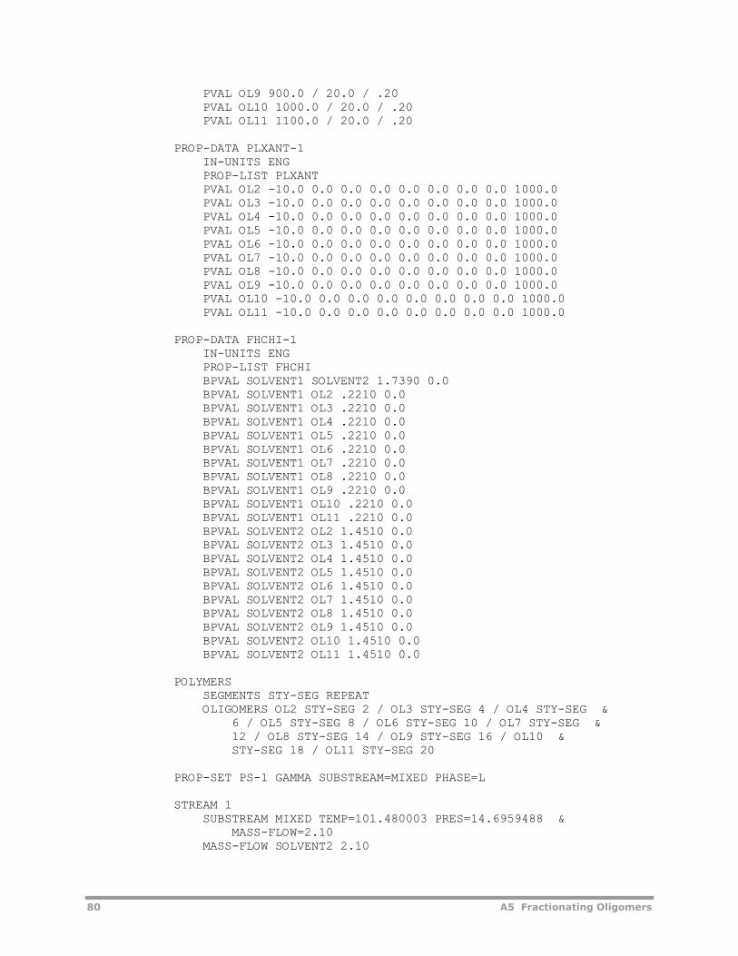
80 A5 Fractionating Oligomers
PVAL OL9 900.0 / 20.0 / .20 PVAL OL10 1000.0 / 20.0 / .20 PVAL OL11 1100.0 / 20.0 / .20 PROP-DATA PLXANT-1 IN-UNITS ENG PROP-LIST PLXANT PVAL OL2 -10.0 0.0 0.0 0.0 0.0 0.0 0.0 0.0 1000.0 PVAL OL3 -10.0 0.0 0.0 0.0 0.0 0.0 0.0 0.0 1000.0 PVAL OL4 -10.0 0.0 0.0 0.0 0.0 0.0 0.0 0.0 1000.0 PVAL OL5 -10.0 0.0 0.0 0.0 0.0 0.0 0.0 0.0 1000.0 PVAL OL6 -10.0 0.0 0.0 0.0 0.0 0.0 0.0 0.0 1000.0 PVAL OL7 -10.0 0.0 0.0 0.0 0.0 0.0 0.0 0.0 1000.0 PVAL OL8 -10.0 0.0 0.0 0.0 0.0 0.0 0.0 0.0 1000.0 PVAL OL9 -10.0 0.0 0.0 0.0 0.0 0.0 0.0 0.0 1000.0 PVAL OL10 -10.0 0.0 0.0 0.0 0.0 0.0 0.0 0.0 1000.0 PVAL OL11 -10.0 0.0 0.0 0.0 0.0 0.0 0.0 0.0 1000.0 PROP-DATA FHCHI-1 IN-UNITS ENG PROP-LIST FHCHI BPVAL SOLVENT1 SOLVENT2 1.7390 0.0 BPVAL SOLVENT1 OL2 .2210 0.0 BPVAL SOLVENT1 OL3 .2210 0.0 BPVAL SOLVENT1 OL4 .2210 0.0 BPVAL SOLVENT1 OL5 .2210 0.0 BPVAL SOLVENT1 OL6 .2210 0.0 BPVAL SOLVENT1 OL7 .2210 0.0 BPVAL SOLVENT1 OL8 .2210 0.0 BPVAL SOLVENT1 OL9 .2210 0.0 BPVAL SOLVENT1 OL10 .2210 0.0 BPVAL SOLVENT1 OL11 .2210 0.0 BPVAL SOLVENT2 OL2 1.4510 0.0 BPVAL SOLVENT2 OL3 1.4510 0.0 BPVAL SOLVENT2 OL4 1.4510 0.0 BPVAL SOLVENT2 OL5 1.4510 0.0 BPVAL SOLVENT2 OL6 1.4510 0.0 BPVAL SOLVENT2 OL7 1.4510 0.0 BPVAL SOLVENT2 OL8 1.4510 0.0 BPVAL SOLVENT2 OL9 1.4510 0.0 BPVAL SOLVENT2 OL10 1.4510 0.0 BPVAL SOLVENT2 OL11 1.4510 0.0 POLYMERS SEGMENTS STY-SEG REPEAT OLIGOMERS OL2 STY-SEG 2 / OL3 STY-SEG 4 / OL4 STY-SEG & 6 / OL5 STY-SEG 8 / OL6 STY-SEG 10 / OL7 STY-SEG & 12 / OL8 STY-SEG 14 / OL9 STY-SEG 16 / OL10 & STY-SEG 18 / OL11 STY-SEG 20 PROP-SET PS-1 GAMMA SUBSTREAM=MIXED PHASE=L STREAM 1 SUBSTREAM MIXED TEMP=101.480003 PRES=14.6959488 & MASS-FLOW=2.10 MASS-FLOW SOLVENT2 2.10
A5 Fractionating Oligomers 81
STREAM 1P SUBSTREAM MIXED TEMP=101.480 PRES=14.6959488 MASS-FLOW=1.0 MASS-FRAC SOLVENT1 .708990 / OL2 .020 / OL3 .060 / OL4 & .080 / OL5 .060 / OL6 .040 / OL7 .020 / OL8 .010 & / OL9 .0010 / OL10 .00010 / OL11 .000010 BLOCK B1 FLASH3 PARAM TEMP=101.480003 PRES=14.6959488 L2-COMP=SOLVENT2 STREAM-REPOR MOLEFLOW MASSFLOW MOLEFRAC MASSFRAC PROPERTIES=PS-1
References Wu, A. H., & Prausnitz, J. M. (1990). J. Appl. Pol. Sci., 39, pp. 629-637.
82 A6 Calculating End-Use Properties
A6 Calculating End-Use Properties
This example demonstrates how to use Aspen Polymers Plus to predict important end-use properties including melt-index, intrinsic viscosity and zero-shear viscosity for high-density polyethylene and other polyolefins using user-defined Prop-Set.
The steps covered include:
• Defining the Simulation
• Creating a New Run
• Creating the Process Flowsheet
• Specifying Setup and Global Options
• Specifying and Characterizing Components
• Specifying Physical Properties
• Supplying Process Information
• Creating a Sensitivity Table
• Running the Simulation and Examining the Results
The industry uses a number of empirical correlative models to predict melt index of polyethylene product. End-use properties such as melt index are best implemented as a property set (Prop-Set). A number of built-in Prop-Sets are available in Aspen Plus. In addition, Prop-Sets let you specify a property set with add-on user correlations. When doing this, a user-supplied Fortran subroutine is required to perform the calculations.
Aspen Polymers Plus supplies a user Prop-Set and the corresponding Fortran subroutine for melt index based on the correlations of Karol, Sinclair, and colleagues, (See the End-Use Properties section in Chapter 2 of the Aspen Polymers Plus User Guide, Volume 1) as well as the intrinsic and zero-shear viscosities (Karol, Brown, & Davison, 1973; Sinclair, 1983).
Defining the Simulation In this example you create an Aspen Polymers Plus process model to predict end-use properties, run the simulation, and examine the results.
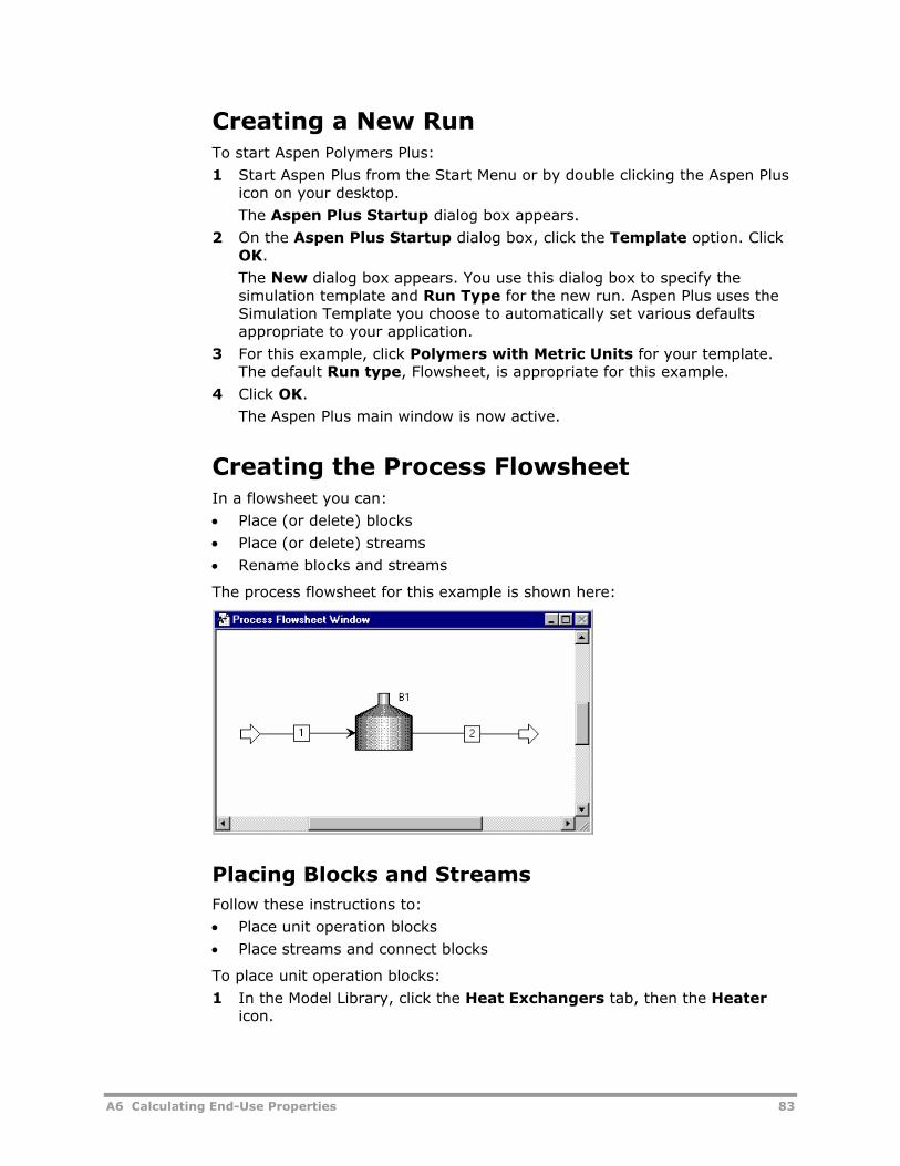
A6 Calculating End-Use Properties 83
Creating a New Run To start Aspen Polymers Plus:
1 Start Aspen Plus from the Start Menu or by double clicking the Aspen Plus icon on your desktop.
The Aspen Plus Startup dialog box appears.
2 On the Aspen Plus Startup dialog box, click the Template option. Click OK.
The New dialog box appears. You use this dialog box to specify the simulation template and Run Type for the new run. Aspen Plus uses the Simulation Template you choose to automatically set various defaults appropriate to your application.
3 For this example, click Polymers with Metric Units for your template. The default Run type, Flowsheet, is appropriate for this example.
4 Click OK.
The Aspen Plus main window is now active.
Creating the Process Flowsheet In a flowsheet you can:
• Place (or delete) blocks
• Place (or delete) streams
• Rename blocks and streams
The process flowsheet for this example is shown here:
Placing Blocks and Streams Follow these instructions to:
• Place unit operation blocks
• Place streams and connect blocks
To place unit operation blocks:
1 In the Model Library, click the Heat Exchangers tab, then the Heater icon.
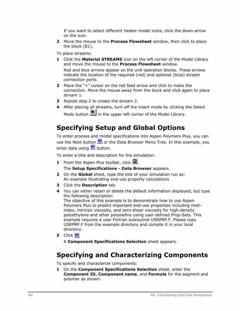
84 A6 Calculating End-Use Properties
If you want to select different Heater model icons, click the down-arrow on the icon.
2 Move the mouse to the Process Flowsheet window, then click to place the block (B1).
To place streams:
1 Click the Material STREAMS icon on the left corner of the Model Library and move the mouse to the Process Flowsheet window.
Red and blue arrows appear on the unit operation blocks. These arrows indicate the location of the required (red) and optional (blue) stream connection ports.
2 Place the “+” cursor on the red feed arrow and click to make the connection. Move the mouse away from the block and click again to place stream 1.
3 Repeat step 2 to create the stream 2.
4 After placing all streams, turn off the insert mode by clicking the Select
Mode button in the upper left corner of the Model Library.
Specifying Setup and Global Options To enter process and model specifications into Aspen Polymers Plus, you can
use the Next button or the Data Browser Menu Tree. In this example, you
enter data using button.
To enter a title and description for the simulation:
1 From the Aspen Plus toolbar, click .
The Setup Specifications - Data Browser appears.
2 On the Global sheet, type the title of your simulation run as: An example illustrating end-use property calculations
3 Click the Description tab.
4 You can either retain or delete the default information displayed, but type the following description: The objective of this example is to demonstrate how to use Aspen Polymers Plus to predict important end-use properties including melt-index, intrinsic viscosity, and zero-shear viscosity for high-density polyethylene and other polyolefins using user-defined Prop-Sets. This example requires a user Fortran subroutine USRPRP.F. Please copy USRPRP.F from the example directory and compile it in your local directory.
5 Click .
A Component Specifications Selection sheet appears.
Specifying and Characterizing Components To specify and characterize components:
1 On the Component Specifications Selection sheet, enter the Component ID, Component name, and Formula for the segment and polymer as shown:
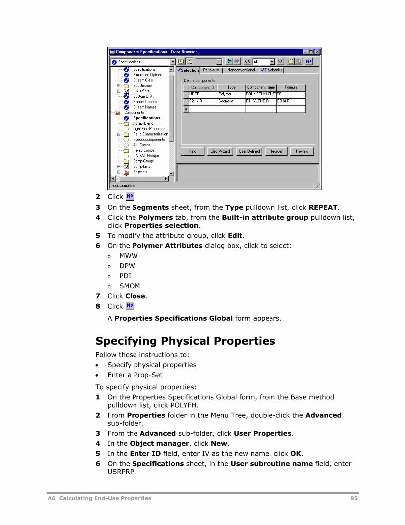
A6 Calculating End-Use Properties 85
2 Click .
3 On the Segments sheet, from the Type pulldown list, click REPEAT.
4 Click the Polymers tab, from the Built-in attribute group pulldown list, click Properties selection.
5 To modify the attribute group, click Edit. 6 On the Polymer Attributes dialog box, click to select:
o MWW
o DPW
o PDI
o SMOM
7 Click Close.
8 Click .
A Properties Specifications Global form appears.
Specifying Physical Properties Follow these instructions to:
• Specify physical properties
• Enter a Prop-Set
To specify physical properties:
1 On the Properties Specifications Global form, from the Base method pulldown list, click POLYFH.
2 From Properties folder in the Menu Tree, double-click the Advanced sub-folder.
3 From the Advanced sub-folder, click User Properties.
4 In the Object manager, click New.
5 In the Enter ID field, enter IV as the new name, click OK.
6 On the Specifications sheet, in the User subroutine name field, enter USRPRP.
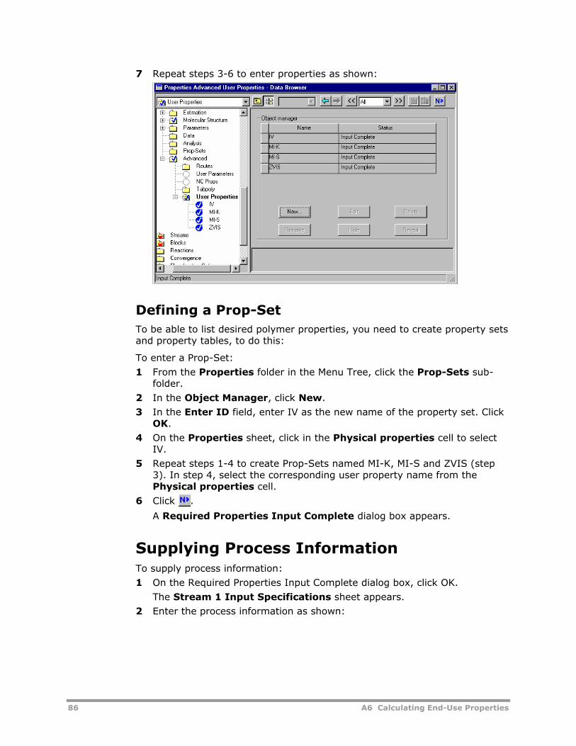
86 A6 Calculating End-Use Properties
7 Repeat steps 3-6 to enter properties as shown:
Defining a Prop-Set To be able to list desired polymer properties, you need to create property sets and property tables, to do this:
To enter a Prop-Set:
1 From the Properties folder in the Menu Tree, click the Prop-Sets sub-folder.
2 In the Object Manager, click New.
3 In the Enter ID field, enter IV as the new name of the property set. Click OK.
4 On the Properties sheet, click in the Physical properties cell to select IV.
5 Repeat steps 1-4 to create Prop-Sets named MI-K, MI-S and ZVIS (step 3). In step 4, select the corresponding user property name from the Physical properties cell.
6 Click .
A Required Properties Input Complete dialog box appears.
Supplying Process Information To supply process information:
1 On the Required Properties Input Complete dialog box, click OK.
The Stream 1 Input Specifications sheet appears.
2 Enter the process information as shown:
A6 Calculating End-Use Properties 87
3 Click .
The Component Attr. Sheet appears.
4 From the Attribute ID pulldown menu, click DPN, in the Value cell, enter 1000.
5 From the Attribute ID pulldown menu, click SFRAC, in the Value cell, enter 1.
6 From the Attribute ID pulldown menu, click PDI, in the Value cell, enter 3.61
7 Click .
The BLOCK B1 Input Specifications sheet appears.
8 Enter:
o Temperature = 420K
o Pressure = 1 atm
Creating a Sensitivity Table To create a sensitivity table:
1 In the Menu Tree, double-click the Model Analysis Tools folder.
2 Click the Sensitivity sub-folder.
3 In the Object manager, click New.
4 In the Enter ID field, enter END-USE as the ID. Click OK.
5 On the Define sheet, click New.
6 In the Enter Variable name field, enter IV. Click OK.
7 In the Variable Definition dialog box, select:
o Category = Streams
o Reference Type = Stream-Prop
o Stream = 2
o Prop-Set = IV
8 Click Close.
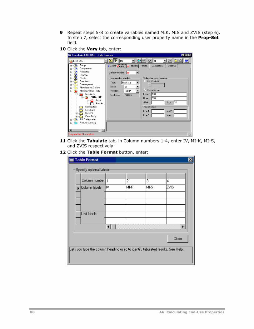
88 A6 Calculating End-Use Properties
9 Repeat steps 5-8 to create variables named MIK, MIS and ZVIS (step 6). In step 7, select the corresponding user property name in the Prop-Set field.
10 Click the Vary tab, enter:
11 Click the Tabulate tab, in Column numbers 1-4, enter IV, MI-K, MI-S,
and ZVIS respectively.
12 Click the Table Format button, enter:
A6 Calculating End-Use Properties 89
Running the Simulation and Examining the Results Note: This example requires a user subroutine, USRPRP.f. You need to copy the Fortran subroutine USRPRP.F from the Aspen Polymers Plus application folder to your working directory. You then need to compile the subroutine before running this example. Alternately, you can copy the files USERFORT.DLL and USERFORT.DLOPT from the Aspen Polymers Plus application folder (app) to your working directory. Then, from the Aspen Plus menu bar, chose Run | Settings | Engine Files and enter USERFORT.DLOPT in the Linker Options box before running the simulation.
Follow these instructions to:
• Run the simulation
• Examine the results
To run the simulation:
1 From the Aspen Plus toolbar, click .
The Control Panel appears.
2 To run the simulation, click .
As the run proceeds, status messages appear in the Control Panel. When the calculations are complete, the message Results Available appears in the status bar at the right corner of the Aspen Plus main window.
To examine the results:
1 From the Menu Tree, double-click the Results Summary folder.
The Summary sheet appears.
2 From the pulldown list between the and buttons, click Results.
3 Click to navigate to the next form with results.
Input Summary The input language summary for this example is shown here:
TITLE 'An example illustrating end-use property calculations' IN-UNITS MET DEF-STREAMS CONVEN ALL DESCRIPTION "The objective of this example is to demonstrate how to use Aspen Polymers Plus to predict important end-use properties including melt-index, intrinsic viscosity, and zero-shear viscosity for high-density polyethylene and other polyolefins using user-defined PROP-SETS. This example requires a user Fortran subroutine USRPRP.F.
90 A6 Calculating End-Use Properties
Please copy USRPRP.F from the example directory and compile it in your local directory." DATABANKS POLYMER / SEGMENT / PURE11 / NOASPENPCD PROP-SOURCES POLYMER / SEGMENT / PURE11 COMPONENTS HDPE PE / C2H4-R C2H4-R FLOWSHEET BLOCK B1 IN=1 OUT=2 PROPERTIES POLYFH POLYMERS SEGMENTS C2H4-R REPEAT POLYMERS HDPE ATTRIBUTES HDPE SFRAC SFLOW DPN DPW PDI MWN MWW ZMOM & FMOM SMOM USER-PROPERT IV SUBROUTINE=USRPRP USER-PROPERT MI-K SUBROUTINE=USRPRP USER-PROPERT MI-S SUBROUTINE=USRPRP USER-PROPERT ZVIS SUBROUTINE=USRPRP PROP-SET IV IV SUBSTREAM=MIXED PROP-SET MI-K MI-K SUBSTREAM=MIXED PROP-SET MI-S MI-S SUBSTREAM=MIXED PROP-SET ZVIS ZVIS SUBSTREAM=MIXED STREAM 1 SUBSTREAM MIXED TEMP=420. <K> PRES=1. MASS-FLOW HDPE 1000. COMP-ATTR HDPE SFRAC ( 1. ) COMP-ATTR HDPE DPN ( 1000. ) COMP-ATTR HDPE PDI ( 3.61 ) BLOCK B1 HEATER PARAM TEMP=420. <K> PRES=1. EO-CONV-OPTI SENSITIVITY END-USE DEFINE IV STREAM-PROP STREAM=2 PROPERTY=IV DEFINE MIK STREAM-PROP STREAM=2 PROPERTY=MI-K DEFINE MIS STREAM-PROP STREAM=2 PROPERTY=MI-S DEFINE ZVIS STREAM-PROP STREAM=2 PROPERTY=ZVIS TABULATE 1 "IV" COL-LABEL="IV" TABULATE 2 "MI-K" COL-LABEL="MI-K"
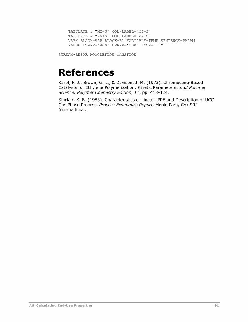
A6 Calculating End-Use Properties 91
TABULATE 3 "MI-S" COL-LABEL="MI-S" TABULATE 4 "ZVIS" COL-LABEL="ZVIS" VARY BLOCK-VAR BLOCK=B1 VARIABLE=TEMP SENTENCE=PARAM RANGE LOWER="400" UPPER="500" INCR="10" STREAM-REPOR NOMOLEFLOW MASSFLOW
References Karol, F. J., Brown, G. L., & Davison, J. M. (1973). Chromocene-Based Catalysts for Ethylene Polymerization: Kinetic Parameters. J. of Polymer Science: Polymer Chemistry Edition, 11, pp. 413-424.
Sinclair, K. B. (1983). Characteristics of Linear LPPE and Description of UCC Gas Phase Process. Process Economics Report. Menlo Park, CA: SRI International.
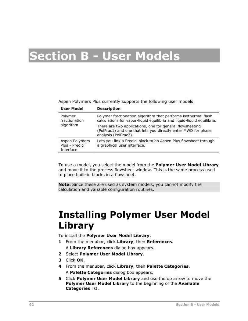
92 Section B - User Models
Section B - User Models
Aspen Polymers Plus currently supports the following user models:
User Model Description
Polymer fractionation algorithm
Polymer fractionation algorithm that performs isothermal flash calculations for vapor-liquid equilibria and liquid-liquid equilibria.
There are two applications, one for general flowsheeting (PolFrac1) and one that lets you directly enter MWD for phase analysis (PolFrac2).
Aspen Polymers Plus - Predici Interface
Lets you link a Predici block to an Aspen Plus flowsheet through a graphical user interface.
To use a model, you select the model from the Polymer User Model Library and move it to the process flowsheet window. This is the same process used to place built-in blocks in a flowsheet.
Note: Since these are used as system models, you cannot modify the calculation and variable configuration routines.
Installing Polymer User Model Library To install the Polymer User Model Library:
1 From the menubar, click Library, then References.
A Library References dialog box appears.
2 Select Polymer User Model Library.
3 Click OK.
4 From the menubar, click Library, then Palette Categories.
A Palette Categories dialog box appears.
5 Click Polymer User Model Library and use the up arrow to move the Polymer User Model Library to the beginning of the Available Categories list.
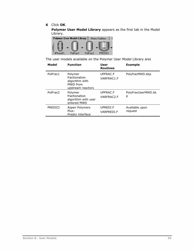
Section B - User Models 93
6 Click OK.
Polymer User Model Library appears as the first tab in the Model Library.
The user models available on the Polymer User Model Library are:
Model Function User Routines
Example
PolFrac1 Polymer fractionation algorithm with MWD from upstream reactors
UPFRAC.F
VARFRAC1.F
PolyfracMWD.bkp
PolFrac2 Polymer fractionation algorithm with user entered MWD
UPFRAC.F
VARFRAC2.F
PolyFracUserMWD.bkp
PREDICI Aspen Polymers Plus– Predici interface
UPREDI.F
VARPREDI.F
Available upon request
94 B1 Polymer Fractionation Algorithm
B1 Polymer Fractionation Algorithm
The polymer fractionation algorithm (PolyFrac) is a polymer flash algorithm based on PolyMix, which was originally developed by the research group of Professor Wolfgang Arlt at the Technology University of Berlin (Behme et al., 2003). PolyFrac performs phase equilibrium calculations for streams containing solvents and polymers. Most importantly, PolyFrac allows a polymer component to possess a molecular weight distribution (MWD), that is, the polydispersity.
The topics covered include:
• Installing the Polymer Fractionation Examples
• Developing a Proprietary Model
• Example Polymer Fractionation Model - PolFrac1
• Example Polymer Fractionation Model - PolFrac2
PolyFrac is implemented as a User2 model in Aspen Polymers Plus and performs isothermal flash calculations for vapor-liquid equilibria and liquid-liquid equilibria using a pseudo-component approach. The algorithm is able to:
• Decompose feed polymer molecular weight distribution curves into a set of pseudo-components
• Perform efficient flash calculations based on these pseudo-components
• Reconstruct the polymer molecular weight distribution curves from pseudo-components for polymers in different phases
There are some restrictions for the model, namely the:
• System can only handle one polymer
• Maximum limit of components is 50 (not including segments)
• Maximum MWD points are 1000
The computation time is practically independent of the number of pseudo-components used to mimic the molecular weight distribution. The model currently supports both the SAFT and PC-SAFT equations-of-state and provides two types of applications in Aspen Polymers Plus, PolFrac1 and PolFrac2. PolFrac1 is for general flowsheeting. PolFrac2 provides an interface that lets you directly enter MWD for phase analysis.
B1 Polymer Fractionation Algorithm 95
Installing the Polymer Fractionation Examples The following files support the polymer fractionation user models:
File Name File Type
polyfracMWD.bkp Template backup file using MWD generated by upstream reactors
PolyfracUserMWD.bkp Template backup file using user-entered MWD
Polymer User Model Library.apm Polymer User Model Library/Model Library file
PolyUserModelLib.dll Polymer User Model Library/User DLL file
Polfrac2.ocx Polymer User Model Library/Customized GUI
Creating a Working Directory To install the model:
1 Create a clean user working directory, such as:
c:\polyfrac
2 Find the folder: Program Files\Aspentech\Aspen Plus 2004.1\GUI\xmp\Aspen Polymers Plus
3 From this folder, copy the two backup files listed in the table above to the working directory you created in step 1.
Developing a Proprietary Model In this example, a template file is created for the polymer fractionation model. You can open the template file to do a test run and replace the existing flowsheet, component, and streams with your own.
Opening the Model To start the model:
1 Go to your working directory, for example c:\polyfrac.
2 Double-click the polyfracMWD.bkp (or polyfracUSerMWD.bkp) file.
The Aspen Plus main window is now active.
Specifying Pseudo-Componenets To change the number of pseudo-components:
1 From the Data Browser, double-click the Components folder, then the Polymers sub-folder.
2 Click the Distributions form.
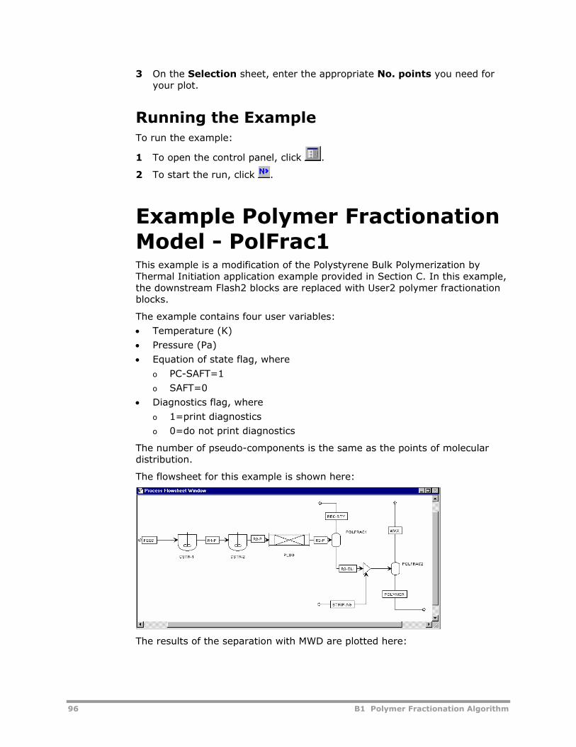
96 B1 Polymer Fractionation Algorithm
3 On the Selection sheet, enter the appropriate No. points you need for your plot.
Running the Example To run the example:
1 To open the control panel, click .
2 To start the run, click .
Example Polymer Fractionation Model - PolFrac1 This example is a modification of the Polystyrene Bulk Polymerization by Thermal Initiation application example provided in Section C. In this example, the downstream Flash2 blocks are replaced with User2 polymer fractionation blocks.
The example contains four user variables:
• Temperature (K)
• Pressure (Pa)
• Equation of state flag, where
o PC-SAFT=1
o SAFT=0
• Diagnostics flag, where
o 1=print diagnostics
o 0=do not print diagnostics
The number of pseudo-components is the same as the points of molecular distribution.
The flowsheet for this example is shown here:
The results of the separation with MWD are plotted here:
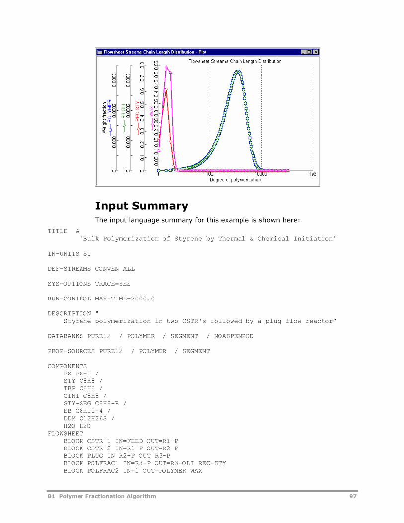
B1 Polymer Fractionation Algorithm 97
Input Summary The input language summary for this example is shown here:
TITLE & 'Bulk Polymerization of Styrene by Thermal & Chemical Initiation' IN-UNITS SI DEF-STREAMS CONVEN ALL SYS-OPTIONS TRACE=YES RUN-CONTROL MAX-TIME=2000.0 DESCRIPTION " Styrene polymerization in two CSTR's followed by a plug flow reactor” DATABANKS PURE12 / POLYMER / SEGMENT / NOASPENPCD PROP-SOURCES PURE12 / POLYMER / SEGMENT COMPONENTS PS PS-1 / STY C8H8 / TBP C8H8 / CINI C8H8 / STY-SEG C8H8-R / EB C8H10-4 / DDM C12H26S / H2O H2O FLOWSHEET BLOCK CSTR-1 IN=FEED OUT=R1-P BLOCK CSTR-2 IN=R1-P OUT=R2-P BLOCK PLUG IN=R2-P OUT=R3-P BLOCK POLFRAC1 IN=R3-P OUT=R3-OLI REC-STY BLOCK POLFRAC2 IN=1 OUT=POLYMER WAX
98 B1 Polymer Fractionation Algorithm
BLOCK MIXER IN=STRIP-AG R3-OLI OUT=1 PROPERTIES POLYPCSF PROPERTIES POLYPCSF / POLYNRTL / POLYSAFT PROP-DATA DATA1 IN-UNITS SI PROP-LIST MW / TB PVAL TBP 216.320 / 2000.0 PVAL DDM 330.0 / 2000.0 PROP-DATA PCSAFT IN-UNITS SI PROP-LIST PCSFTM / PCSFTU / PCSFTV PVAL STY 3.0 / 285 / 3.75 PVAL TBP 3.0 / 285 / 3.75 PVAL CINI 3.0 / 285 / 3.75 PVAL EB 3.0 / 285 / 3.75 PVAL DDM 3.0 / 285 / 3.75 PVAL H2O 3.0 / 285 / 3.75 PROP-LIST PCSFTU / PCSFTV / PCSFTR PVAL PS 267 / 4.1071 / 0.0190 PROP-DATA PURE-1 IN-UNITS SI PROP-LIST SAFTM / SAFTU / SAFTV PVAL STY 4.7 / 245 / .013 PVAL EB 4.719 / 248.79 / .01268 PVAL PS 1000 / 210 / .012 PVAL TBP 5 / 300 / .05 PVAL CINI 3 / 300 / .03 PVAL DDM 3 / 300 / .03 PVAL H2O 1 / 400 / .018 PROP-DATA PLXANT-1 IN-UNITS SI PROP-LIST PLXANT PVAL TBP -30.0 0.0 0.0 0.0 0.0 0.0 0.0 0.0 1000.0 PVAL DDM -30.0 0.0 0.0 0.0 0.0 0.0 0.0 0.0 1000.0 PROP-DATA PCSKIJ-1 IN-UNITS SI PROP-LIST PCSKIJ BPVAL PS STY 0.05 POLYMERS SEGMENTS STY-SEG REPEAT POLYMERS PS ATTRIBUTES PS SFRAC SFLOW DPN DPW PDI MWN MWW ZMOM FMOM & SMOM LDPN LZMOM LFMOM LSFLOW LSFRAC LEFLOW LEFRAC & LPFRAC DISTRIBUTION PS CHAIN-SIZE NPOINTS=200 FUNCLOG=NO & UPPER=100000. STREAM FEED SUBSTREAM MIXED TEMP=298.150 PRES=101325.0 MASS-FLOW=1.94440 & NPHASE=1 PHASE=L MASS-FRAC STY .980 / TBP .000250 / EB .019370 / DDM &
B1 Polymer Fractionation Algorithm 99
.00060 STREAM STRIP-AG SUBSTREAM MIXED TEMP=298.150 PRES=202650.0 MASS-FLOW=.040 & NPHASE=1 PHASE=L MASS-FLOW H2O .040 BLOCK MIXER MIXER PARAM PRES=1. <atm> NPHASE=1 PHASE=L PROPERTIES POLYPCSF BLOCK-OPTION FREE-WATER=NO BLOCK CSTR-1 RCSTR PARAM VOL=20.0 TEMP=393.150 PRES=101325.0 NPHASE=1 PHASE=L & MB-MAXIT=200 MB-TOL=.000010 REACTIONS RXN-IDS=R1 BLOCK CSTR-2 RCSTR PARAM VOL=20.0 TEMP=433.150 PRES=101325.0 NPHASE=1 PHASE=L & MB-MAXIT=400 MB-TOL=.000010 REACTIONS RXN-IDS=R1 BLOCK PLUG RPLUG PARAM TYPE=T-SPEC LENGTH=80.0 DIAM=.40 PHASE=L & PRES=101325.0 NPOINT=100 HINIT=1.0000E-07 INT-TOL=.0010 & CORR-METHOD=DIRECT T-SPEC 0.0 433.150 / 1.0 473.150 REACTIONS RXN-IDS=R1 BLOCK POLFRAC1 USER2 SUBROUTINE UPFRAC PARAM NINT=2 NREAL=2 NCHAR=2 INT VALUE-LIST=1 1 REAL VALUE-LIST=493.15 101325. CHAR & CHAR-LIST="INT: (0) SAFT (1) PCSAFT-----REAL: TEMPERATURE IN DEG K" & "INT: (1) PRINT DIAGNOSTICS----REAL: PRESSURE IN PASCAL" PROPERTIES POLYPCSF / POLYPCSF BLOCK POLFRAC2 USER2 SUBROUTINE UPFRAC PARAM NINT=2 NREAL=2 NCHAR=2 INT VALUE-LIST=1 1 REAL VALUE-LIST=493.15 70000. CHAR & CHAR-LIST="INT: (0) SAFT (1) PCSAFT-----REAL: TEMPERATURE IN DEG K" & "INT: (1) PRINT DIAGNOSTICS----REAL: PRESSURE IN PASCAL" PROPERTIES POLYPCSF / POLYPCSF EO-CONV-OPTI CONV-OPTIONS PARAM CHECKSEQ=NO STREAM-REPOR MOLEFLOW MASSFLOW MASSFRAC REACTIONS R1 FREE-RAD DESCRIPTION "Free-Radical Kinetic Scheme"
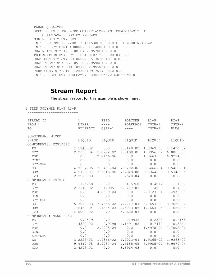
100 B1 Polymer Fractionation Algorithm
PARAM QSSA=YES SPECIES INITIATOR=TBP COINITIATOR=CINI MONOMER=STY & CHAINTAG=EB DDM POLYMER=PS MON-RSEG STY STY-SEG INIT-DEC TBP 1.6220E+11 1.1530E+08 0.0 EFFIC=.80 NRADS=2 INIT-SP STY CINI 438000.0 1.1480E+08 0.0 CHAIN-INI STY 1.0510E+07 2.9570E+07 0.0 PROPAGATION STY STY 1.0510E+07 2.9570E+07 0.0 CHAT-MON STY STY 3310000.0 5.3020E+07 0.0 CHAT-AGENT STY EB 1051.0 2.9590E+07 0.0 CHAT-AGENT STY DDM 1051.0 2.9590E+07 0.0 TERM-COMB STY STY 1.2550E+09 7017000.0 0.0 INIT-SP-EFF STY COEFFA=0.0 COEFFB=3.0 COEFFC=0.0
Stream Report The stream report for this example is shown here:
1 FEED POLYMER R1-P R2-P ------------------------ STREAM ID 1 FEED POLYMER R1-P R2-P FROM : MIXER ---- POLFRAC2 CSTR-1 CSTR-2 TO : POLFRAC2 CSTR-1 ---- CSTR-2 PLUG SUBSTREAM: MIXED PHASE: LIQUID LIQUID LIQUID LIQUID LIQUID COMPONENTS: KMOL/SEC PS 1.5140-02 0.0 1.5140-02 4.3369-03 1.1490-02 STY 2.2965-04 1.8292-02 1.7490-05 1.3956-02 6.8065-03 TBP 0.0 2.2466-06 0.0 1.3463-06 6.9214-08 CINI 0.0 0.0 0.0 0.0 0.0 STY-SEG 0.0 0.0 0.0 0.0 0.0 EB 4.9967-05 3.5467-04 7.3202-06 3.5466-04 3.5463-04 DDM 4.9795-07 3.5345-06 7.2949-08 3.5344-06 3.5340-06 H2O 2.2203-03 0.0 3.2528-04 0.0 0.0 COMPONENTS: KG/SEC PS 1.5768 0.0 1.5768 0.4517 1.1967 STY 2.3918-02 1.9051 1.8217-03 1.4536 0.7089 TBP 0.0 4.8599-04 0.0 2.9123-04 1.4972-05 CINI 0.0 0.0 0.0 0.0 0.0 STY-SEG 0.0 0.0 0.0 0.0 0.0 EB 5.3049-03 3.7655-02 7.7717-04 3.7654-02 3.7650-02 DDM 1.6432-04 1.1664-03 2.4073-05 1.1663-03 1.1662-03 H2O 4.0000-02 0.0 5.8600-03 0.0 0.0 COMPONENTS: MASS FRAC PS 0.9579 0.0 0.9946 0.2323 0.6154 STY 1.4529-02 0.9798 1.1491-03 0.7476 0.3646 TBP 0.0 2.4995-04 0.0 1.4978-04 7.7002-06 CINI 0.0 0.0 0.0 0.0 0.0 STY-SEG 0.0 0.0 0.0 0.0 0.0 EB 3.2225-03 1.9366-02 4.9023-04 1.9365-02 1.9363-02 DDM 9.9819-05 5.9987-04 1.5185-05 5.9985-04 5.9979-04 H2O 2.4298-02 0.0 3.6964-03 0.0 0.0
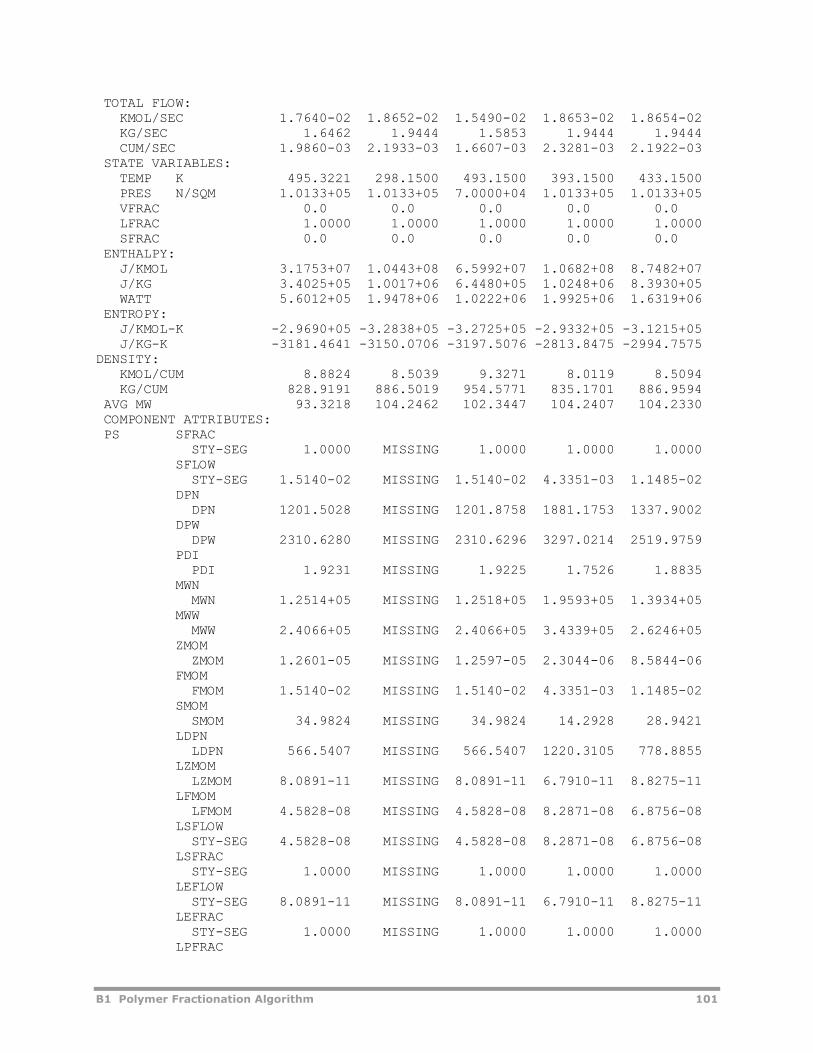
B1 Polymer Fractionation Algorithm 101
TOTAL FLOW: KMOL/SEC 1.7640-02 1.8652-02 1.5490-02 1.8653-02 1.8654-02 KG/SEC 1.6462 1.9444 1.5853 1.9444 1.9444 CUM/SEC 1.9860-03 2.1933-03 1.6607-03 2.3281-03 2.1922-03 STATE VARIABLES: TEMP K 495.3221 298.1500 493.1500 393.1500 433.1500 PRES N/SQM 1.0133+05 1.0133+05 7.0000+04 1.0133+05 1.0133+05 VFRAC 0.0 0.0 0.0 0.0 0.0 LFRAC 1.0000 1.0000 1.0000 1.0000 1.0000 SFRAC 0.0 0.0 0.0 0.0 0.0 ENTHALPY: J/KMOL 3.1753+07 1.0443+08 6.5992+07 1.0682+08 8.7482+07 J/KG 3.4025+05 1.0017+06 6.4480+05 1.0248+06 8.3930+05 WATT 5.6012+05 1.9478+06 1.0222+06 1.9925+06 1.6319+06 ENTROPY: J/KMOL-K -2.9690+05 -3.2838+05 -3.2725+05 -2.9332+05 -3.1215+05 J/KG-K -3181.4641 -3150.0706 -3197.5076 -2813.8475 -2994.7575 DENSITY: KMOL/CUM 8.8824 8.5039 9.3271 8.0119 8.5094 KG/CUM 828.9191 886.5019 954.5771 835.1701 886.9594 AVG MW 93.3218 104.2462 102.3447 104.2407 104.2330 COMPONENT ATTRIBUTES: PS SFRAC STY-SEG 1.0000 MISSING 1.0000 1.0000 1.0000 SFLOW STY-SEG 1.5140-02 MISSING 1.5140-02 4.3351-03 1.1485-02 DPN DPN 1201.5028 MISSING 1201.8758 1881.1753 1337.9002 DPW DPW 2310.6280 MISSING 2310.6296 3297.0214 2519.9759 PDI PDI 1.9231 MISSING 1.9225 1.7526 1.8835 MWN MWN 1.2514+05 MISSING 1.2518+05 1.9593+05 1.3934+05 MWW MWW 2.4066+05 MISSING 2.4066+05 3.4339+05 2.6246+05 ZMOM ZMOM 1.2601-05 MISSING 1.2597-05 2.3044-06 8.5844-06 FMOM FMOM 1.5140-02 MISSING 1.5140-02 4.3351-03 1.1485-02 SMOM SMOM 34.9824 MISSING 34.9824 14.2928 28.9421 LDPN LDPN 566.5407 MISSING 566.5407 1220.3105 778.8855 LZMOM LZMOM 8.0891-11 MISSING 8.0891-11 6.7910-11 8.8275-11 LFMOM LFMOM 4.5828-08 MISSING 4.5828-08 8.2871-08 6.8756-08 LSFLOW STY-SEG 4.5828-08 MISSING 4.5828-08 8.2871-08 6.8756-08 LSFRAC STY-SEG 1.0000 MISSING 1.0000 1.0000 1.0000 LEFLOW STY-SEG 8.0891-11 MISSING 8.0891-11 6.7910-11 8.8275-11 LEFRAC STY-SEG 1.0000 MISSING 1.0000 1.0000 1.0000 LPFRAC
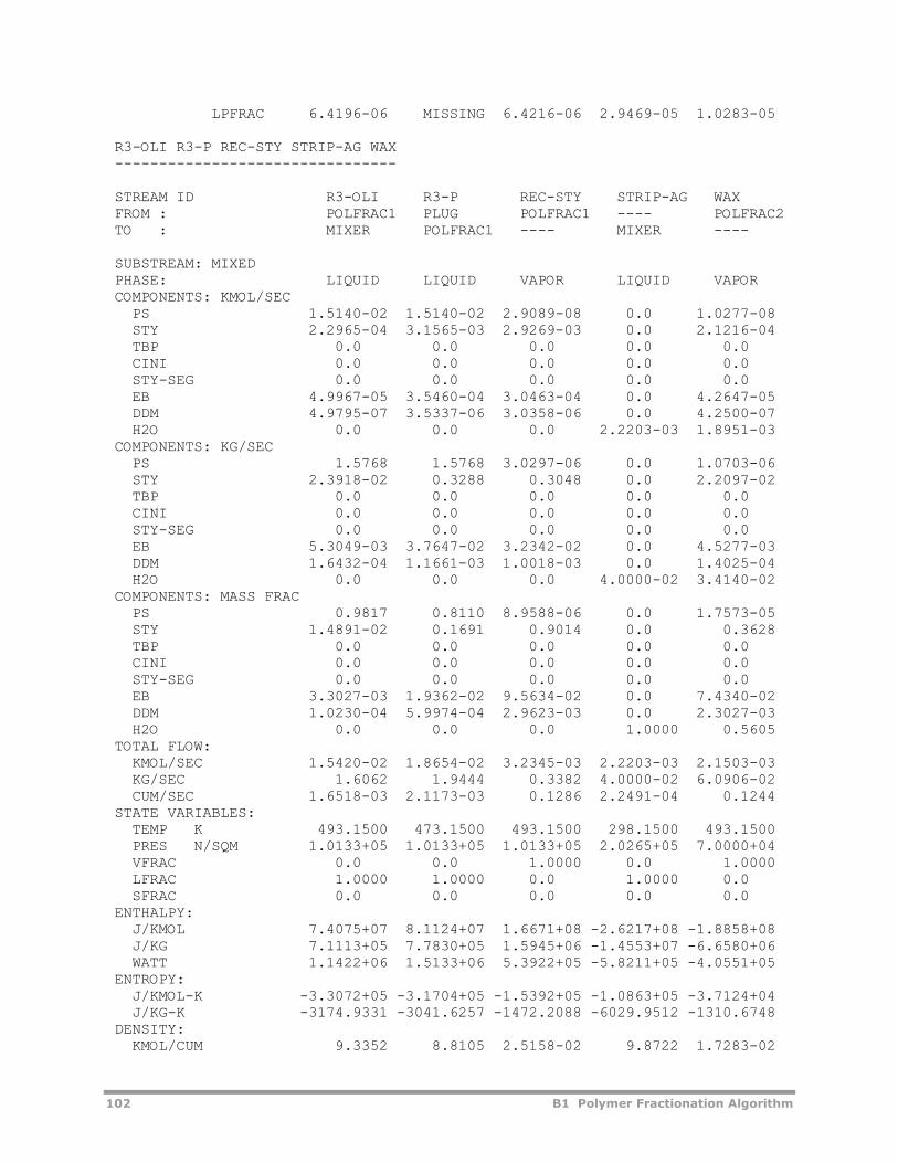
102 B1 Polymer Fractionation Algorithm
LPFRAC 6.4196-06 MISSING 6.4216-06 2.9469-05 1.0283-05 R3-OLI R3-P REC-STY STRIP-AG WAX -------------------------------- STREAM ID R3-OLI R3-P REC-STY STRIP-AG WAX FROM : POLFRAC1 PLUG POLFRAC1 ---- POLFRAC2 TO : MIXER POLFRAC1 ---- MIXER ---- SUBSTREAM: MIXED PHASE: LIQUID LIQUID VAPOR LIQUID VAPOR COMPONENTS: KMOL/SEC PS 1.5140-02 1.5140-02 2.9089-08 0.0 1.0277-08 STY 2.2965-04 3.1565-03 2.9269-03 0.0 2.1216-04 TBP 0.0 0.0 0.0 0.0 0.0 CINI 0.0 0.0 0.0 0.0 0.0 STY-SEG 0.0 0.0 0.0 0.0 0.0 EB 4.9967-05 3.5460-04 3.0463-04 0.0 4.2647-05 DDM 4.9795-07 3.5337-06 3.0358-06 0.0 4.2500-07 H2O 0.0 0.0 0.0 2.2203-03 1.8951-03 COMPONENTS: KG/SEC PS 1.5768 1.5768 3.0297-06 0.0 1.0703-06 STY 2.3918-02 0.3288 0.3048 0.0 2.2097-02 TBP 0.0 0.0 0.0 0.0 0.0 CINI 0.0 0.0 0.0 0.0 0.0 STY-SEG 0.0 0.0 0.0 0.0 0.0 EB 5.3049-03 3.7647-02 3.2342-02 0.0 4.5277-03 DDM 1.6432-04 1.1661-03 1.0018-03 0.0 1.4025-04 H2O 0.0 0.0 0.0 4.0000-02 3.4140-02 COMPONENTS: MASS FRAC PS 0.9817 0.8110 8.9588-06 0.0 1.7573-05 STY 1.4891-02 0.1691 0.9014 0.0 0.3628 TBP 0.0 0.0 0.0 0.0 0.0 CINI 0.0 0.0 0.0 0.0 0.0 STY-SEG 0.0 0.0 0.0 0.0 0.0 EB 3.3027-03 1.9362-02 9.5634-02 0.0 7.4340-02 DDM 1.0230-04 5.9974-04 2.9623-03 0.0 2.3027-03 H2O 0.0 0.0 0.0 1.0000 0.5605 TOTAL FLOW: KMOL/SEC 1.5420-02 1.8654-02 3.2345-03 2.2203-03 2.1503-03 KG/SEC 1.6062 1.9444 0.3382 4.0000-02 6.0906-02 CUM/SEC 1.6518-03 2.1173-03 0.1286 2.2491-04 0.1244 STATE VARIABLES: TEMP K 493.1500 473.1500 493.1500 298.1500 493.1500 PRES N/SQM 1.0133+05 1.0133+05 1.0133+05 2.0265+05 7.0000+04 VFRAC 0.0 0.0 1.0000 0.0 1.0000 LFRAC 1.0000 1.0000 0.0 1.0000 0.0 SFRAC 0.0 0.0 0.0 0.0 0.0 ENTHALPY: J/KMOL 7.4075+07 8.1124+07 1.6671+08 -2.6217+08 -1.8858+08 J/KG 7.1113+05 7.7830+05 1.5945+06 -1.4553+07 -6.6580+06 WATT 1.1422+06 1.5133+06 5.3922+05 -5.8211+05 -4.0551+05 ENTROPY: J/KMOL-K -3.3072+05 -3.1704+05 -1.5392+05 -1.0863+05 -3.7124+04 J/KG-K -3174.9331 -3041.6257 -1472.2088 -6029.9512 -1310.6748 DENSITY: KMOL/CUM 9.3352 8.8105 2.5158-02 9.8722 1.7283-02
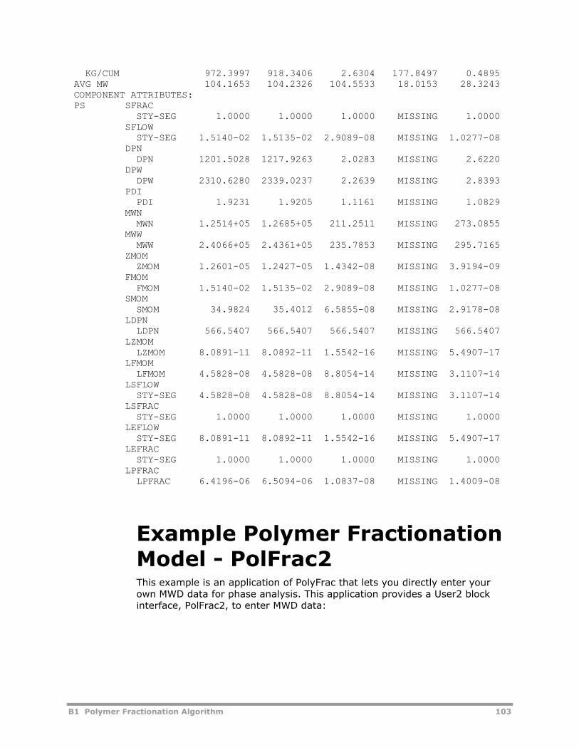
B1 Polymer Fractionation Algorithm 103
KG/CUM 972.3997 918.3406 2.6304 177.8497 0.4895 AVG MW 104.1653 104.2326 104.5533 18.0153 28.3243 COMPONENT ATTRIBUTES: PS SFRAC STY-SEG 1.0000 1.0000 1.0000 MISSING 1.0000 SFLOW STY-SEG 1.5140-02 1.5135-02 2.9089-08 MISSING 1.0277-08 DPN DPN 1201.5028 1217.9263 2.0283 MISSING 2.6220 DPW DPW 2310.6280 2339.0237 2.2639 MISSING 2.8393 PDI PDI 1.9231 1.9205 1.1161 MISSING 1.0829 MWN MWN 1.2514+05 1.2685+05 211.2511 MISSING 273.0855 MWW MWW 2.4066+05 2.4361+05 235.7853 MISSING 295.7165 ZMOM ZMOM 1.2601-05 1.2427-05 1.4342-08 MISSING 3.9194-09 FMOM FMOM 1.5140-02 1.5135-02 2.9089-08 MISSING 1.0277-08 SMOM SMOM 34.9824 35.4012 6.5855-08 MISSING 2.9178-08 LDPN LDPN 566.5407 566.5407 566.5407 MISSING 566.5407 LZMOM LZMOM 8.0891-11 8.0892-11 1.5542-16 MISSING 5.4907-17 LFMOM LFMOM 4.5828-08 4.5828-08 8.8054-14 MISSING 3.1107-14 LSFLOW STY-SEG 4.5828-08 4.5828-08 8.8054-14 MISSING 3.1107-14 LSFRAC STY-SEG 1.0000 1.0000 1.0000 MISSING 1.0000 LEFLOW STY-SEG 8.0891-11 8.0892-11 1.5542-16 MISSING 5.4907-17 LEFRAC STY-SEG 1.0000 1.0000 1.0000 MISSING 1.0000 LPFRAC LPFRAC 6.4196-06 6.5094-06 1.0837-08 MISSING 1.4009-08
Example Polymer Fractionation Model - PolFrac2 This example is an application of PolyFrac that lets you directly enter your own MWD data for phase analysis. This application provides a User2 block interface, PolFrac2, to enter MWD data:
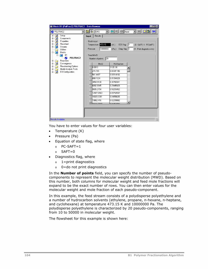
104 B1 Polymer Fractionation Algorithm
You have to enter values for four user variables:
• Temperature (K)
• Pressure (Pa)
• Equation of state flag, where o PC-SAFT=1
o SAFT=0
• Diagnostics flag, where
o 1=print diagnostics
o 0=do not print diagnostics
In the Number of points field, you can specify the number of pseudo-components to represent the molecular weight distribution (MWD). Based on this number, both columns for molecular weight and feed mole fractions will expand to be the exact number of rows. You can then enter values for the molecular weight and mole fraction of each pseudo-component.
In this example, the feed stream consists of a polydisperse polyethylene and a number of hydrocarbon solvents (ethylene, propane, n-hexane, n-heptane, and cyclohexane) at temperature 473.15 K and 10000000 Pa. The polydisperse polyethylene is characterized by 20 pseudo-components, ranging from 10 to 50000 in molecular weight.
The flowsheet for this example is shown here:
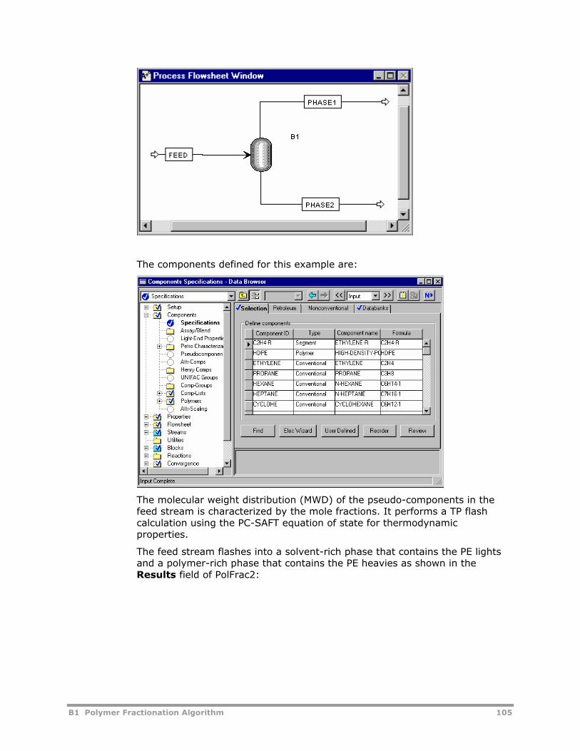
B1 Polymer Fractionation Algorithm 105
The components defined for this example are:
The molecular weight distribution (MWD) of the pseudo-components in the feed stream is characterized by the mole fractions. It performs a TP flash calculation using the PC-SAFT equation of state for thermodynamic properties.
The feed stream flashes into a solvent-rich phase that contains the PE lights and a polymer-rich phase that contains the PE heavies as shown in the Results field of PolFrac2:
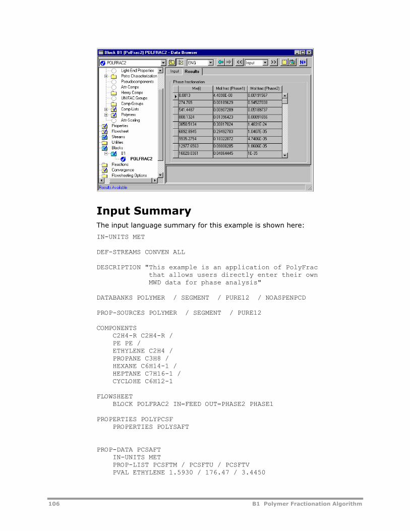
106 B1 Polymer Fractionation Algorithm
Input Summary The input language summary for this example is shown here:
IN-UNITS MET DEF-STREAMS CONVEN ALL DESCRIPTION "This example is an application of PolyFrac that allows users directly enter their own MWD data for phase analysis" DATABANKS POLYMER / SEGMENT / PURE12 / NOASPENPCD PROP-SOURCES POLYMER / SEGMENT / PURE12 COMPONENTS C2H4-R C2H4-R / PE PE / ETHYLENE C2H4 / PROPANE C3H8 / HEXANE C6H14-1 / HEPTANE C7H16-1 / CYCLOHE C6H12-1 FLOWSHEET BLOCK POLFRAC2 IN=FEED OUT=PHASE2 PHASE1 PROPERTIES POLYPCSF PROPERTIES POLYSAFT PROP-DATA PCSAFT IN-UNITS MET PROP-LIST PCSFTM / PCSFTU / PCSFTV PVAL ETHYLENE 1.5930 / 176.47 / 3.4450
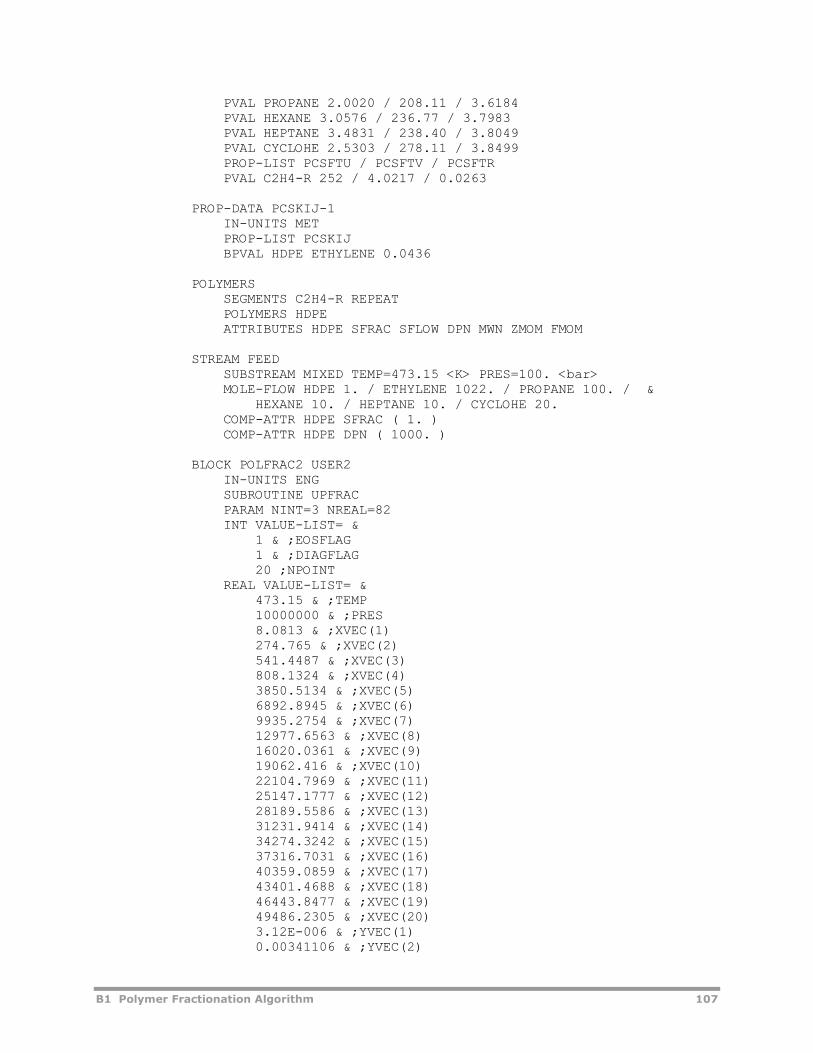
B1 Polymer Fractionation Algorithm 107
PVAL PROPANE 2.0020 / 208.11 / 3.6184 PVAL HEXANE 3.0576 / 236.77 / 3.7983 PVAL HEPTANE 3.4831 / 238.40 / 3.8049 PVAL CYCLOHE 2.5303 / 278.11 / 3.8499 PROP-LIST PCSFTU / PCSFTV / PCSFTR PVAL C2H4-R 252 / 4.0217 / 0.0263 PROP-DATA PCSKIJ-1 IN-UNITS MET PROP-LIST PCSKIJ BPVAL HDPE ETHYLENE 0.0436 POLYMERS SEGMENTS C2H4-R REPEAT POLYMERS HDPE ATTRIBUTES HDPE SFRAC SFLOW DPN MWN ZMOM FMOM STREAM FEED SUBSTREAM MIXED TEMP=473.15 <K> PRES=100. <bar> MOLE-FLOW HDPE 1. / ETHYLENE 1022. / PROPANE 100. / & HEXANE 10. / HEPTANE 10. / CYCLOHE 20. COMP-ATTR HDPE SFRAC ( 1. ) COMP-ATTR HDPE DPN ( 1000. ) BLOCK POLFRAC2 USER2 IN-UNITS ENG SUBROUTINE UPFRAC PARAM NINT=3 NREAL=82 INT VALUE-LIST= & 1 & ;EOSFLAG 1 & ;DIAGFLAG 20 ;NPOINT REAL VALUE-LIST= & 473.15 & ;TEMP 10000000 & ;PRES 8.0813 & ;XVEC(1) 274.765 & ;XVEC(2) 541.4487 & ;XVEC(3) 808.1324 & ;XVEC(4) 3850.5134 & ;XVEC(5) 6892.8945 & ;XVEC(6) 9935.2754 & ;XVEC(7) 12977.6563 & ;XVEC(8) 16020.0361 & ;XVEC(9) 19062.416 & ;XVEC(10) 22104.7969 & ;XVEC(11) 25147.1777 & ;XVEC(12) 28189.5586 & ;XVEC(13) 31231.9414 & ;XVEC(14) 34274.3242 & ;XVEC(15) 37316.7031 & ;XVEC(16) 40359.0859 & ;XVEC(17) 43401.4688 & ;XVEC(18) 46443.8477 & ;XVEC(19) 49486.2305 & ;XVEC(20) 3.12E-006 & ;YVEC(1) 0.00341106 & ;YVEC(2)
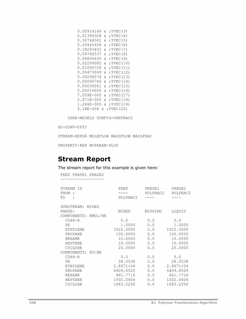
108 B1 Polymer Fractionation Algorithm
0.00914166 & ;YVEC(3) 0.01394328 & ;YVEC(4) 0.30768341 & ;YVEC(5) 0.29445428 & ;YVEC(6) 0.18293452 & ;YVEC(7) 0.09792537 & ;YVEC(8) 0.04856635 & ;YVEC(9) 0.02299082 & ;YVEC(10) 0.01054726 & ;YVEC(11) 0.00473049 & ;YVEC(12) 0.00208576 & ;YVEC(13) 0.00090746 & ;YVEC(14) 0.00039061 & ;YVEC(15) 0.00016666 & ;YVEC(16) 7.059E-005 & ;YVEC(17) 2.971E-005 & ;YVEC(18) 1.244E-005 & ;YVEC(19) 5.18E-006 & ;YVEC(20) USER-MODELS CONFIG=VARFRAC2 EO-CONV-OPTI STREAM-REPOR MOLEFLOW MASSFLOW MASSFRAC PROPERTY-REP NOPARAM-PLUS
Stream Report The stream report for this example is given here:
FEED PHASE1 PHASE2 ------------------ STREAM ID FEED PHASE1 PHASE2 FROM : ---- POLFRAC2 POLFRAC2 TO : POLFRAC2 ---- ---- SUBSTREAM: MIXED PHASE: MIXED MISSING LIQUID COMPONENTS: KMOL/HR C2H4-R 0.0 0.0 0.0 PE 1.0000 0.0 1.0000 ETHYLENE 1022.0000 0.0 1022.0000 PROPANE 100.0000 0.0 100.0000 HEXANE 10.0000 0.0 10.0000 HEPTANE 10.0000 0.0 10.0000 CYCLOHE 20.0000 0.0 20.0000 COMPONENTS: KG/HR C2H4-R 0.0 0.0 0.0 PE 28.0538 0.0 28.0538 ETHYLENE 2.8671+04 0.0 2.8671+04 PROPANE 4409.6520 0.0 4409.6520 HEXANE 861.7716 0.0 861.7716 HEPTANE 1002.0404 0.0 1002.0404 CYCLOHE 1683.2256 0.0 1683.2256
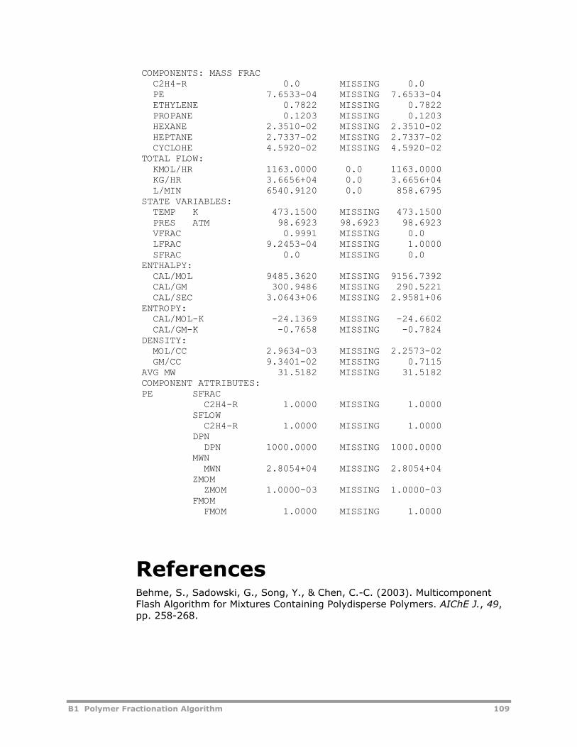
B1 Polymer Fractionation Algorithm 109
COMPONENTS: MASS FRAC C2H4-R 0.0 MISSING 0.0 PE 7.6533-04 MISSING 7.6533-04 ETHYLENE 0.7822 MISSING 0.7822 PROPANE 0.1203 MISSING 0.1203 HEXANE 2.3510-02 MISSING 2.3510-02 HEPTANE 2.7337-02 MISSING 2.7337-02 CYCLOHE 4.5920-02 MISSING 4.5920-02 TOTAL FLOW: KMOL/HR 1163.0000 0.0 1163.0000 KG/HR 3.6656+04 0.0 3.6656+04 L/MIN 6540.9120 0.0 858.6795 STATE VARIABLES: TEMP K 473.1500 MISSING 473.1500 PRES ATM 98.6923 98.6923 98.6923 VFRAC 0.9991 MISSING 0.0 LFRAC 9.2453-04 MISSING 1.0000 SFRAC 0.0 MISSING 0.0 ENTHALPY: CAL/MOL 9485.3620 MISSING 9156.7392 CAL/GM 300.9486 MISSING 290.5221 CAL/SEC 3.0643+06 MISSING 2.9581+06 ENTROPY: CAL/MOL-K -24.1369 MISSING -24.6602 CAL/GM-K -0.7658 MISSING -0.7824 DENSITY: MOL/CC 2.9634-03 MISSING 2.2573-02 GM/CC 9.3401-02 MISSING 0.7115 AVG MW 31.5182 MISSING 31.5182 COMPONENT ATTRIBUTES: PE SFRAC C2H4-R 1.0000 MISSING 1.0000 SFLOW C2H4-R 1.0000 MISSING 1.0000 DPN DPN 1000.0000 MISSING 1000.0000 MWN MWN 2.8054+04 MISSING 2.8054+04 ZMOM ZMOM 1.0000-03 MISSING 1.0000-03 FMOM FMOM 1.0000 MISSING 1.0000
References Behme, S., Sadowski, G., Song, Y., & Chen, C.-C. (2003). Multicomponent Flash Algorithm for Mixtures Containing Polydisperse Polymers. AIChE J., 49, pp. 258-268.
110 B2 Aspen Polymers Plus-Predici Interface
B2 Aspen Polymers Plus-Predici Interface
Modeling of complex polymerization processes requires a detailed description of the thermophysical properties, chemical kinetics, unit operation models, and flowsheeting capabilities of a simulator. Aspen Polymers Plus provides these features, while Predici provides useful descriptions of kinetics and polymer molecular weight distribution. The Aspen Polymers Plus-Predici interface lets you combine the strengths of both packages.
The Aspen Polymers Plus-Predici interface lets you enter the Predici model name, working directory, connections between Aspen stream and Predici reactors, and mapping between Aspen component name and Predici alias name. It also supports data transfer between Aspen and Predici through COM technology.
This example demonstrates how to integrate a Predici model in Aspen Plus as a flowsheet reactor block.
The topics covered include:
• Developing a Proprietary Model
• Example Predici Four CSTR Model
Developing a Proprietary Model The Aspen Polymers Plus-Predici interface is included in the Polymer User Model Library as the PREDICI model.
Opening the Model To start the Aspen Polymers Plus-Predici model:
1 From the menubar, click Library, then References.
A Library References dialog box appears.
2 Select Polymer User Model Library.
3 Click OK.
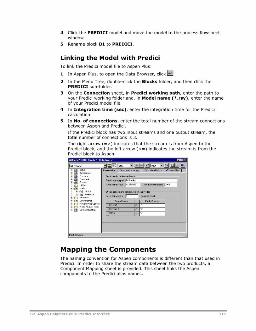
B2 Aspen Polymers Plus-Predici Interface 111
4 Click the PREDICI model and move the model to the process flowsheet window.
5 Rename block B1 to PREDICI.
Linking the Model with Predici To link the Predici model file to Aspen Plus:
1 In Aspen Plus, to open the Data Browser, click .
2 In the Menu Tree, double-click the Blocks folder, and then click the PREDICI sub-folder.
3 On the Connection sheet, in Predici working path, enter the path to your Predici working folder and, in Model name (*.rsy), enter the name of your Predici model file.
4 In Integration time (sec), enter the integration time for the Predici calculation.
5 In No. of connections, enter the total number of the stream connections between Aspen and Predici.
If the Predici block has two input streams and one output stream, the total number of connections is 3.
The right arrow (=>) indicates that the stream is from Aspen to the Predici block, and the left arrow (<=) indicates the stream is from the Predici block to Aspen.
Mapping the Components The naming convention for Aspen components is different than that used in Predici. In order to share the stream data between the two products, a Component Mapping sheet is provided. This sheet links the Aspen components to the Predici alias names.
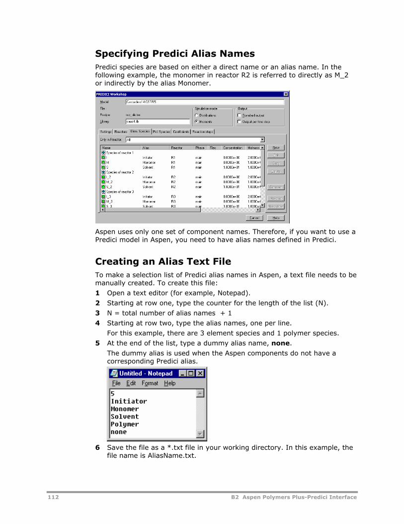
112 B2 Aspen Polymers Plus-Predici Interface
Specifying Predici Alias Names Predici species are based on either a direct name or an alias name. In the following example, the monomer in reactor R2 is referred to directly as M_2 or indirectly by the alias Monomer.
Aspen uses only one set of component names. Therefore, if you want to use a Predici model in Aspen, you need to have alias names defined in Predici.
Creating an Alias Text File To make a selection list of Predici alias names in Aspen, a text file needs to be manually created. To create this file:
1 Open a text editor (for example, Notepad).
2 Starting at row one, type the counter for the length of the list (N).
3 N = total number of alias names + 1
4 Starting at row two, type the alias names, one per line.
For this example, there are 3 element species and 1 polymer species.
5 At the end of the list, type a dummy alias name, none.
The dummy alias is used when the Aspen components do not have a corresponding Predici alias.
6 Save the file as a *.txt file in your working directory. In this example, the
file name is AliasName.txt.
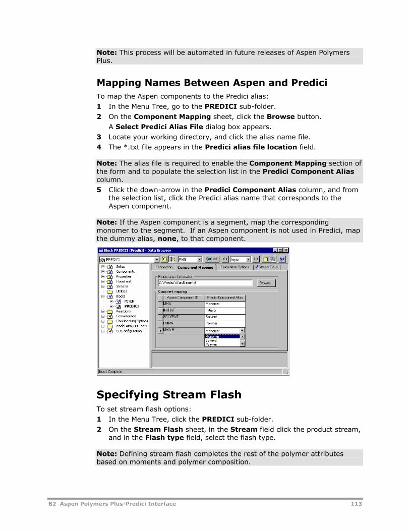
B2 Aspen Polymers Plus-Predici Interface 113
Note: This process will be automated in future releases of Aspen Polymers Plus.
Mapping Names Between Aspen and Predici To map the Aspen components to the Predici alias:
1 In the Menu Tree, go to the PREDICI sub-folder.
2 On the Component Mapping sheet, click the Browse button.
A Select Predici Alias File dialog box appears.
3 Locate your working directory, and click the alias name file.
4 The *.txt file appears in the Predici alias file location field.
Note: The alias file is required to enable the Component Mapping section of the form and to populate the selection list in the Predici Component Alias column.
5 Click the down-arrow in the Predici Component Alias column, and from the selection list, click the Predici alias name that corresponds to the Aspen component.
Note: If the Aspen component is a segment, map the corresponding monomer to the segment. If an Aspen component is not used in Predici, map the dummy alias, none, to that component.
Specifying Stream Flash To set stream flash options:
1 In the Menu Tree, click the PREDICI sub-folder.
2 On the Stream Flash sheet, in the Stream field click the product stream, and in the Flash type field, select the flash type.
Note: Defining stream flash completes the rest of the polymer attributes based on moments and polymer composition.
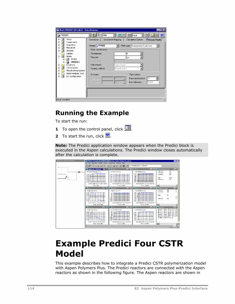
114 B2 Aspen Polymers Plus-Predici Interface
Running the Example To start the run:
1 To open the control panel, click .
2 To start the run, click .
Note: The Predici application window appears when the Predici block is executed in the Aspen calculations. The Predici window closes automatically after the calculation is complete.
Example Predici Four CSTR Model This example describes how to integrate a Predici CSTR polymerization model with Aspen Polymers Plus. The Predici reactors are connected with the Aspen reactors as shown in the following figure. The Aspen reactors are shown in
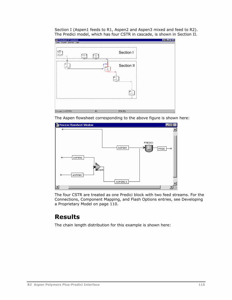
B2 Aspen Polymers Plus-Predici Interface 115
Section I (Aspen1 feeds to R1, Aspen2 and Aspen3 mixed and feed to R2). The Predici model, which has four CSTR in cascade, is shown in Section II.
The Aspen flowsheet corresponding to the above figure is shown here:
The four CSTR are treated as one Predici block with two feed streams. For the Connections, Component Mapping, and Flash Options entries, see Developing a Proprietary Model on page 110.
Results The chain length distribution for this example is shown here:
Section I
Section II
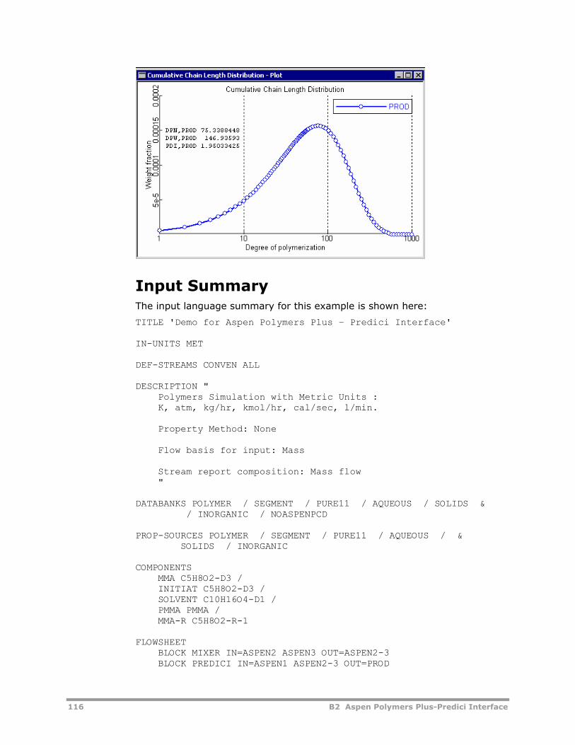
116 B2 Aspen Polymers Plus-Predici Interface
Input Summary The input language summary for this example is shown here:
TITLE 'Demo for Aspen Polymers Plus – Predici Interface' IN-UNITS MET DEF-STREAMS CONVEN ALL DESCRIPTION " Polymers Simulation with Metric Units : K, atm, kg/hr, kmol/hr, cal/sec, l/min. Property Method: None Flow basis for input: Mass Stream report composition: Mass flow " DATABANKS POLYMER / SEGMENT / PURE11 / AQUEOUS / SOLIDS & / INORGANIC / NOASPENPCD PROP-SOURCES POLYMER / SEGMENT / PURE11 / AQUEOUS / & SOLIDS / INORGANIC COMPONENTS MMA C5H8O2-D3 / INITIAT C5H8O2-D3 / SOLVENT C10H16O4-D1 / PMMA PMMA / MMA-R C5H8O2-R-1 FLOWSHEET BLOCK MIXER IN=ASPEN2 ASPEN3 OUT=ASPEN2-3 BLOCK PREDICI IN=ASPEN1 ASPEN2-3 OUT=PROD
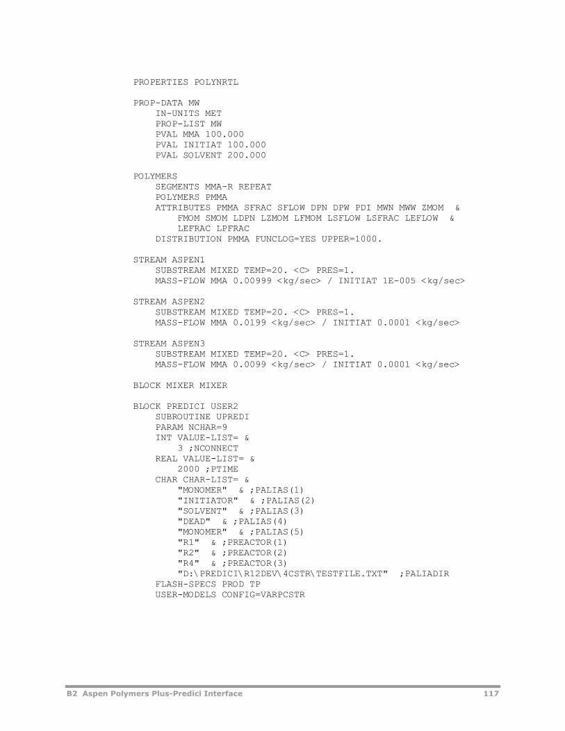
B2 Aspen Polymers Plus-Predici Interface 117
PROPERTIES POLYNRTL PROP-DATA MW IN-UNITS MET PROP-LIST MW PVAL MMA 100.000 PVAL INITIAT 100.000 PVAL SOLVENT 200.000 POLYMERS SEGMENTS MMA-R REPEAT POLYMERS PMMA ATTRIBUTES PMMA SFRAC SFLOW DPN DPW PDI MWN MWW ZMOM & FMOM SMOM LDPN LZMOM LFMOM LSFLOW LSFRAC LEFLOW & LEFRAC LPFRAC DISTRIBUTION PMMA FUNCLOG=YES UPPER=1000. STREAM ASPEN1 SUBSTREAM MIXED TEMP=20. <C> PRES=1. MASS-FLOW MMA 0.00999 <kg/sec> / INITIAT 1E-005 <kg/sec> STREAM ASPEN2 SUBSTREAM MIXED TEMP=20. <C> PRES=1. MASS-FLOW MMA 0.0199 <kg/sec> / INITIAT 0.0001 <kg/sec> STREAM ASPEN3 SUBSTREAM MIXED TEMP=20. <C> PRES=1. MASS-FLOW MMA 0.0099 <kg/sec> / INITIAT 0.0001 <kg/sec> BLOCK MIXER MIXER BLOCK PREDICI USER2 SUBROUTINE UPREDI PARAM NCHAR=9 INT VALUE-LIST= & 3 ;NCONNECT REAL VALUE-LIST= & 2000 ;PTIME CHAR CHAR-LIST= & "MONOMER" & ;PALIAS(1) "INITIATOR" & ;PALIAS(2) "SOLVENT" & ;PALIAS(3) "DEAD" & ;PALIAS(4) "MONOMER" & ;PALIAS(5) "R1" & ;PREACTOR(1) "R2" & ;PREACTOR(2) "R4" & ;PREACTOR(3) "D:\PREDICI\R12DEV\4CSTR\TESTFILE.TXT" ;PALIADIR FLASH-SPECS PROD TP USER-MODELS CONFIG=VARPCSTR
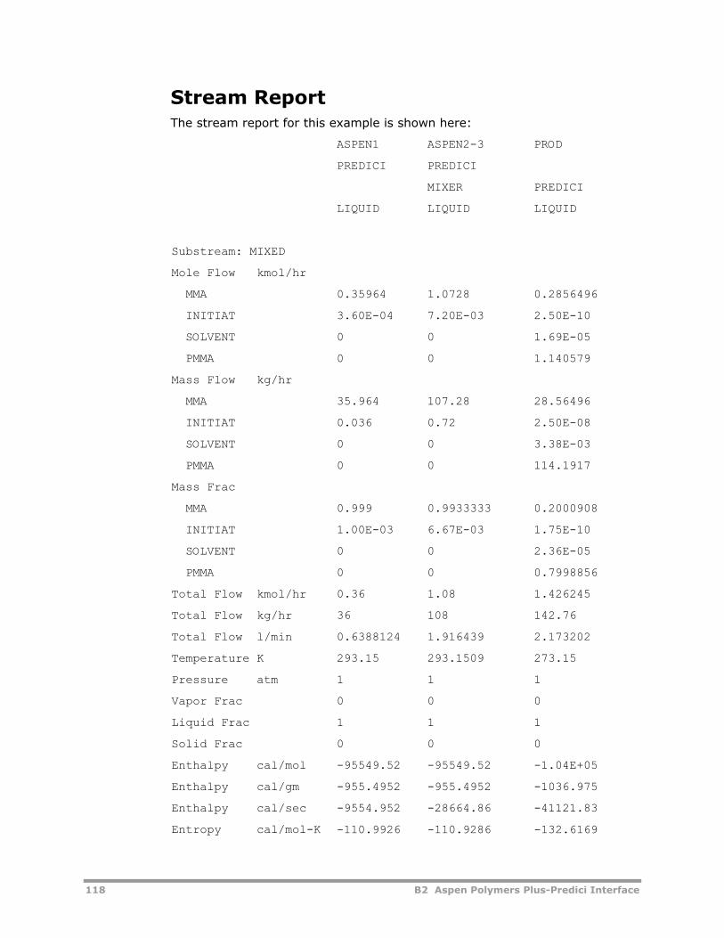
118 B2 Aspen Polymers Plus-Predici Interface
Stream Report The stream report for this example is shown here:
ASPEN1 ASPEN2-3 PROD
PREDICI PREDICI
MIXER PREDICI
LIQUID LIQUID LIQUID
Substream: MIXED
Mole Flow kmol/hr
MMA 0.35964 1.0728 0.2856496
INITIAT 3.60E-04 7.20E-03 2.50E-10
SOLVENT 0 0 1.69E-05
PMMA 0 0 1.140579
Mass Flow kg/hr
MMA 35.964 107.28 28.56496
INITIAT 0.036 0.72 2.50E-08
SOLVENT 0 0 3.38E-03
PMMA 0 0 114.1917
Mass Frac
MMA 0.999 0.9933333 0.2000908
INITIAT 1.00E-03 6.67E-03 1.75E-10
SOLVENT 0 0 2.36E-05
PMMA 0 0 0.7998856
Total Flow kmol/hr 0.36 1.08 1.426245
Total Flow kg/hr 36 108 142.76
Total Flow l/min 0.6388124 1.916439 2.173202
Temperature K 293.15 293.1509 273.15
Pressure atm 1 1 1
Vapor Frac 0 0 0
Liquid Frac 1 1 1
Solid Frac 0 0 0
Enthalpy cal/mol -95549.52 -95549.52 -1.04E+05
Enthalpy cal/gm -955.4952 -955.4952 -1036.975
Enthalpy cal/sec -9554.952 -28664.86 -41121.83
Entropy cal/mol-K -110.9926 -110.9286 -132.6169
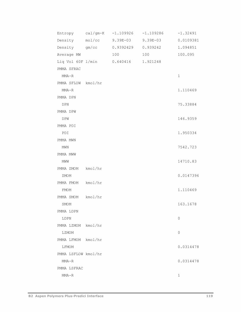
B2 Aspen Polymers Plus-Predici Interface 119
Entropy cal/gm-K -1.109926 -1.109286 -1.32491
Density mol/cc 9.39E-03 9.39E-03 0.0109381
Density gm/cc 0.9392429 0.939242 1.094851
Average MW 100 100 100.095
Liq Vol 60F l/min 0.640416 1.921248
PMMA SFRAC
MMA-R 1
PMMA SFLOW kmol/hr
MMA-R 1.110469
PMMA DPN
DPN 75.33884
PMMA DPW
DPW 146.9359
PMMA PDI
PDI 1.950334
PMMA MWN
MWN 7542.723
PMMA MWW
MWW 14710.83
PMMA ZMOM kmol/hr
ZMOM 0.0147396
PMMA FMOM kmol/hr
FMOM 1.110469
PMMA SMOM kmol/hr
SMOM 163.1678
PMMA LDPN
LDPN 0
PMMA LZMOM kmol/hr
LZMOM 0
PMMA LFMOM kmol/hr
LFMOM 0.0314478
PMMA LSFLOW kmol/hr
MMA-R 0.0314478
PMMA LSFRAC
MMA-R 1

120 B2 Aspen Polymers Plus-Predici Interface
C1 Polystyrene Bulk Polymerization by Thermal Initiation
The polystyrene bulk polymerization by thermal initiation model illustrates the use of Aspen Polymers Plus for modeling free-radical bulk polymerization of styrene with thermal and peroxide initiation. The part of the process modeled is the polymerization stage and subsequent devolatilization. This model is used to study the effect of feed flow rate on styrene conversion, polymer properties, and recycle flowrate.
About This Process Typically in free-radical polymerization, an initiator decomposes to form free radicals that initiate chain growth. Propagation reactions add successive monomer molecules to a growing polymer chain to increase its chain length. A growing polymer chain terminates by either chain transfer or termination reactions to form dead polymer chains.
Styrene monomer, when heated to polymerization temperatures above 120°C, can generate enough free-radicals to produce high conversion and high molecular weight polymer. Styrene reacts via a Diels-Alder-type mechanism to form dimers that react with an additional styrene molecule to produce free-radicals. The thermal initiation rate has been reported to be third-order in styrene concentration (Hui & Hamielec, 1972).
Process Definition Styrene is polymerized in a reactor train consisting of two CSTRs followed by a plug flow reactor. All of the reactors are considered liquid filled, and are therefore modeled without taking into account vapor-liquid equilibrium. Unreacted monomer is flashed in a devolatilizer to be modeled as an ideal flash unit.
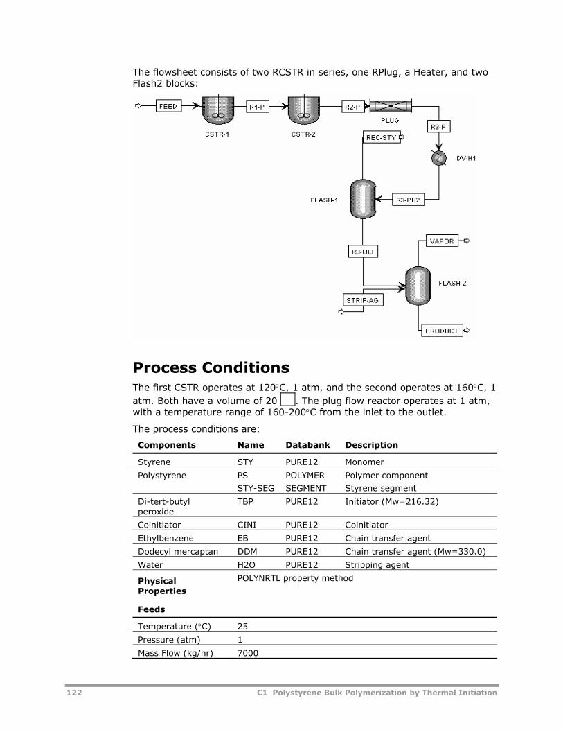
122 C1 Polystyrene Bulk Polymerization by Thermal Initiation
The flowsheet consists of two RCSTR in series, one RPlug, a Heater, and two Flash2 blocks:
Process Conditions The first CSTR operates at 120°C, 1 atm, and the second operates at 160°C, 1 atm. Both have a volume of 20 . The plug flow reactor operates at 1 atm, with a temperature range of 160-200°C from the inlet to the outlet.
The process conditions are:
Components Name Databank Description
Styrene STY PURE12 Monomer
Polystyrene PS
STY-SEG
POLYMER
SEGMENT
Polymer component
Styrene segment
Di-tert-butyl peroxide
TBP PURE12 Initiator (Mw=216.32)
Coinitiator CINI PURE12 Coinitiator
Ethylbenzene EB PURE12 Chain transfer agent
Dodecyl mercaptan DDM PURE12 Chain transfer agent (Mw=330.0)
Water H2O PURE12 Stripping agent
Physical Properties
POLYNRTL property method
Feeds
Temperature (°C) 25
Pressure (atm) 1
Mass Flow (kg/hr) 7000
Mass fraction of styrene
.98
Mass fraction of polystyrene
0.0
Mass fraction of coinitiator
0.0
Mass fraction of ethylbenzene
0.019
Mass fraction of DDM 0.0007
Mass fraction of TBP 0.0003
Kinetics FREE-RAD model
Operating Conditions
Block Temp (°C) Pres (atm) Size
CSTR-1 120 1 20 m3
CSTR-2 160 1 20 m3
PLUG 160-200 1 80 m length by 0.40 m diam
DV-H1 220 1
FLASH-1 220 1
FLASH-2 220 1
Physical Property Models and Data The Polymer Non-Random Two Liquid activity coefficient model physical property method (POLYNRTL) is used. As no parameters are provided, the thermophysical properties (density, heat capacity, etc.) of styrene, ethylbenzene, dodecyl mercaptan, di-tert-butyl peroxide, and water are calculated using parameters from the Pure Component Databank. Note that the coinitiator is given the properties of styrene. However, as this component is used only as a dummy component for the thermal initiation reaction, results are not affected. The polymer thermophysical properties are calculated using the van Krevelen group contribution method.
Reactors / Kinetics The kinetics of bulk and solution polymerization of styrene have been studied extensively. It has been reported (Albright, 1985) that chain transfer to the monomer and the Diels-Alder dimers primarily controls the molecular weight of polystyrene. Furthermore, based on chemical evidence and kinetic modeling, it has been reported that termination of the growing chains occurs principally by combination over disproportionation.
The reactions included from the built-in free-radical kinetics are:
Description Reaction
Initiator decomposition •→ RI
Thermal initiation
124 C1 Polystyrene Bulk Polymerization by Thermal Initiation
Chain initiation
Propagation
Chain transfer to monomer
Chain transfer to EB •+→+ RDEBP nn
Chain transfer to DDM •+→+ RDDDMP nn
Termination by combination
The unit for the rate constant for the thermal initiation reaction is while the unit for the rate constant for initiator decomposition
reaction is 1/s. The units for the rate constants for the other reactions are .
The induced initiation reaction is configured for thermal initiation by setting the power to be third-order with respect to monomer. A coinitiator, which is required for the induced initiation reaction, is included in the list of components, but its power and feed rate are set to zero so that it will not influence the rate for the thermal initiation reaction.
Process Studies The model is used to study the effect of feed flow rate on styrene conversion, polymer properties, and recycle styrene flowrate. In order to determine the effect of feed flowrate on styrene conversion, polymer properties, and recycle flowrate, a sensitivity study is carried out with feed mass flow as the varied parameter.
Input Summary An input language summary for this example is shown here:
; Free radical bulk polymerization of styrene by thermal and chemical ; initiation ; QSSA case ; DYNAPLUS DPLUS RESULTS=ON TITLE & 'Bulk Polymerization of Styrene by Thermal & Chemical Initiation' IN-UNITS MET ENTHALPY-FLO='kcal/hr' PRESSURE=bar TEMPERATURE=C & DELTA-T=C MOLE-ENTHALP='kcal/kmol' MASS-ENTHALP='kcal/kg' & HEAT=kcal PDROP=bar INVERSE-PRES='1/bar' DEF-STREAMS CONVEN ALL SYS-OPTIONS TRACE=YES RUN-CONTROL MAX-TIME=2000.0
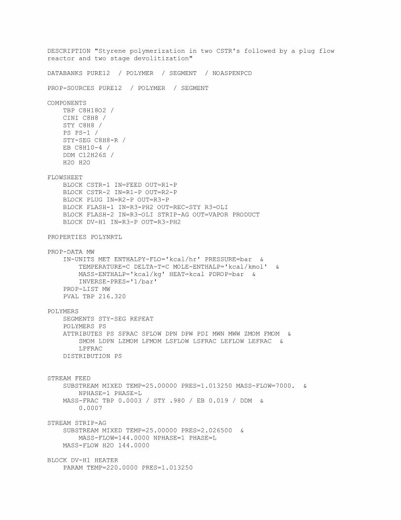
DESCRIPTION "Styrene polymerization in two CSTR's followed by a plug flow reactor and two stage devolitization" DATABANKS PURE12 / POLYMER / SEGMENT / NOASPENPCD PROP-SOURCES PURE12 / POLYMER / SEGMENT COMPONENTS TBP C8H18O2 / CINI C8H8 / STY C8H8 / PS PS-1 / STY-SEG C8H8-R / EB C8H10-4 / DDM C12H26S / H2O H2O FLOWSHEET BLOCK CSTR-1 IN=FEED OUT=R1-P BLOCK CSTR-2 IN=R1-P OUT=R2-P BLOCK PLUG IN=R2-P OUT=R3-P BLOCK FLASH-1 IN=R3-PH2 OUT=REC-STY R3-OLI BLOCK FLASH-2 IN=R3-OLI STRIP-AG OUT=VAPOR PRODUCT BLOCK DV-H1 IN=R3-P OUT=R3-PH2 PROPERTIES POLYNRTL PROP-DATA MW IN-UNITS MET ENTHALPY-FLO='kcal/hr' PRESSURE=bar & TEMPERATURE=C DELTA-T=C MOLE-ENTHALP='kcal/kmol' & MASS-ENTHALP='kcal/kg' HEAT=kcal PDROP=bar & INVERSE-PRES='1/bar' PROP-LIST MW PVAL TBP 216.320 POLYMERS SEGMENTS STY-SEG REPEAT POLYMERS PS ATTRIBUTES PS SFRAC SFLOW DPN DPW PDI MWN MWW ZMOM FMOM & SMOM LDPN LZMOM LFMOM LSFLOW LSFRAC LEFLOW LEFRAC & LPFRAC DISTRIBUTION PS STREAM FEED SUBSTREAM MIXED TEMP=25.00000 PRES=1.013250 MASS-FLOW=7000. & NPHASE=1 PHASE=L MASS-FRAC TBP 0.0003 / STY .980 / EB 0.019 / DDM & 0.0007 STREAM STRIP-AG SUBSTREAM MIXED TEMP=25.00000 PRES=2.026500 & MASS-FLOW=144.0000 NPHASE=1 PHASE=L MASS-FLOW H2O 144.0000 BLOCK DV-H1 HEATER PARAM TEMP=220.0000 PRES=1.013250
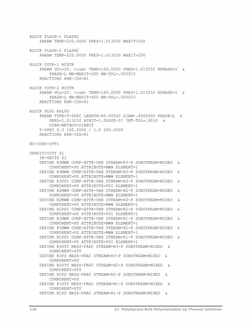
126 C1 Polystyrene Bulk Polymerization by Thermal Initiation
BLOCK FLASH-1 FLASH2 PARAM TEMP=220.0000 PRES=1.013250 MAXIT=200 BLOCK FLASH-2 FLASH2 PARAM TEMP=220.0000 PRES=1.013250 MAXIT=200 BLOCK CSTR-1 RCSTR PARAM VOL=20. <cum> TEMP=120.0000 PRES=1.013250 NPHASE=1 & PHASE=L MB-MAXIT=200 MB-TOL=.000010 REACTIONS RXN-IDS=R1 BLOCK CSTR-2 RCSTR PARAM VOL=20. <cum> TEMP=160.0000 PRES=1.013250 NPHASE=1 & PHASE=L MB-MAXIT=400 MB-TOL=.000010 REACTIONS RXN-IDS=R1 BLOCK PLUG RPLUG PARAM TYPE=T-SPEC LENGTH=80.00000 DIAM=.4000000 PHASE=L & PRES=1.013250 HINIT=1.0000E-07 INT-TOL=.0010 & CORR-METHOD=DIRECT T-SPEC 0.0 160.0000 / 1.0 200.0000 REACTIONS RXN-IDS=R1 EO-CONV-OPTI SENSITIVITY S1 IN-UNITS SI DEFINE R3MWN COMP-ATTR-VAR STREAM=R3-P SUBSTREAM=MIXED & COMPONENT=PS ATTRIBUTE=MWN ELEMENT=1 DEFINE R3MWW COMP-ATTR-VAR STREAM=R3-P SUBSTREAM=MIXED & COMPONENT=PS ATTRIBUTE=MWW ELEMENT=1 DEFINE R3PDI COMP-ATTR-VAR STREAM=R3-P SUBSTREAM=MIXED & COMPONENT=PS ATTRIBUTE=PDI ELEMENT=1 DEFINE R2MWN COMP-ATTR-VAR STREAM=R2-P SUBSTREAM=MIXED & COMPONENT=PS ATTRIBUTE=MWN ELEMENT=1 DEFINE R2MWW COMP-ATTR-VAR STREAM=R2-P SUBSTREAM=MIXED & COMPONENT=PS ATTRIBUTE=MWW ELEMENT=1 DEFINE R2PDI COMP-ATTR-VAR STREAM=R2-P SUBSTREAM=MIXED & COMPONENT=PS ATTRIBUTE=PDI ELEMENT=1 DEFINE R1MWN COMP-ATTR-VAR STREAM=R1-P SUBSTREAM=MIXED & COMPONENT=PS ATTRIBUTE=MWN ELEMENT=1 DEFINE R1MWW COMP-ATTR-VAR STREAM=R1-P SUBSTREAM=MIXED & COMPONENT=PS ATTRIBUTE=MWW ELEMENT=1 DEFINE R1PDI COMP-ATTR-VAR STREAM=R1-P SUBSTREAM=MIXED & COMPONENT=PS ATTRIBUTE=PDI ELEMENT=1 DEFINE R3STY MASS-FRAC STREAM=R3-P SUBSTREAM=MIXED & COMPONENT=STY DEFINE R3PS MASS-FRAC STREAM=R3-P SUBSTREAM=MIXED & COMPONENT=PS DEFINE R2STY MASS-FRAC STREAM=R2-P SUBSTREAM=MIXED & COMPONENT=STY DEFINE R2PS MASS-FRAC STREAM=R2-P SUBSTREAM=MIXED & COMPONENT=PS DEFINE R1STY MASS-FRAC STREAM=R1-P SUBSTREAM=MIXED & COMPONENT=STY DEFINE R1PS MASS-FRAC STREAM=R1-P SUBSTREAM=MIXED &
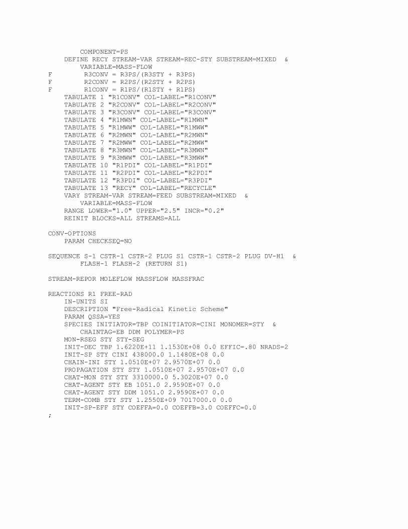
COMPONENT=PS DEFINE RECY STREAM-VAR STREAM=REC-STY SUBSTREAM=MIXED & VARIABLE=MASS-FLOW F R3CONV = R3PS/(R3STY + R3PS) F R2CONV = R2PS/(R2STY + R2PS) F R1CONV = R1PS/(R1STY + R1PS) TABULATE 1 "R1CONV" COL-LABEL="R1CONV" TABULATE 2 "R2CONV" COL-LABEL="R2CONV" TABULATE 3 "R3CONV" COL-LABEL="R3CONV" TABULATE 4 "R1MWN" COL-LABEL="R1MWN" TABULATE 5 "R1MWW" COL-LABEL="R1MWW" TABULATE 6 "R2MWN" COL-LABEL="R2MWN" TABULATE 7 "R2MWW" COL-LABEL="R2MWW" TABULATE 8 "R3MWN" COL-LABEL="R3MWN" TABULATE 9 "R3MWW" COL-LABEL="R3MWW" TABULATE 10 "R1PDI" COL-LABEL="R1PDI" TABULATE 11 "R2PDI" COL-LABEL="R2PDI" TABULATE 12 "R3PDI" COL-LABEL="R3PDI" TABULATE 13 "RECY" COL-LABEL="RECYCLE" VARY STREAM-VAR STREAM=FEED SUBSTREAM=MIXED & VARIABLE=MASS-FLOW RANGE LOWER="1.0" UPPER="2.5" INCR="0.2" REINIT BLOCKS=ALL STREAMS=ALL CONV-OPTIONS PARAM CHECKSEQ=NO SEQUENCE S-1 CSTR-1 CSTR-2 PLUG S1 CSTR-1 CSTR-2 PLUG DV-H1 & FLASH-1 FLASH-2 (RETURN S1) STREAM-REPOR MOLEFLOW MASSFLOW MASSFRAC REACTIONS R1 FREE-RAD IN-UNITS SI DESCRIPTION "Free-Radical Kinetic Scheme" PARAM QSSA=YES SPECIES INITIATOR=TBP COINITIATOR=CINI MONOMER=STY & CHAINTAG=EB DDM POLYMER=PS MON-RSEG STY STY-SEG INIT-DEC TBP 1.6220E+11 1.1530E+08 0.0 EFFIC=.80 NRADS=2 INIT-SP STY CINI 438000.0 1.1480E+08 0.0 CHAIN-INI STY 1.0510E+07 2.9570E+07 0.0 PROPAGATION STY STY 1.0510E+07 2.9570E+07 0.0 CHAT-MON STY STY 3310000.0 5.3020E+07 0.0 CHAT-AGENT STY EB 1051.0 2.9590E+07 0.0 CHAT-AGENT STY DDM 1051.0 2.9590E+07 0.0 TERM-COMB STY STY 1.2550E+09 7017000.0 0.0 INIT-SP-EFF STY COEFFA=0.0 COEFFB=3.0 COEFFC=0.0 ;
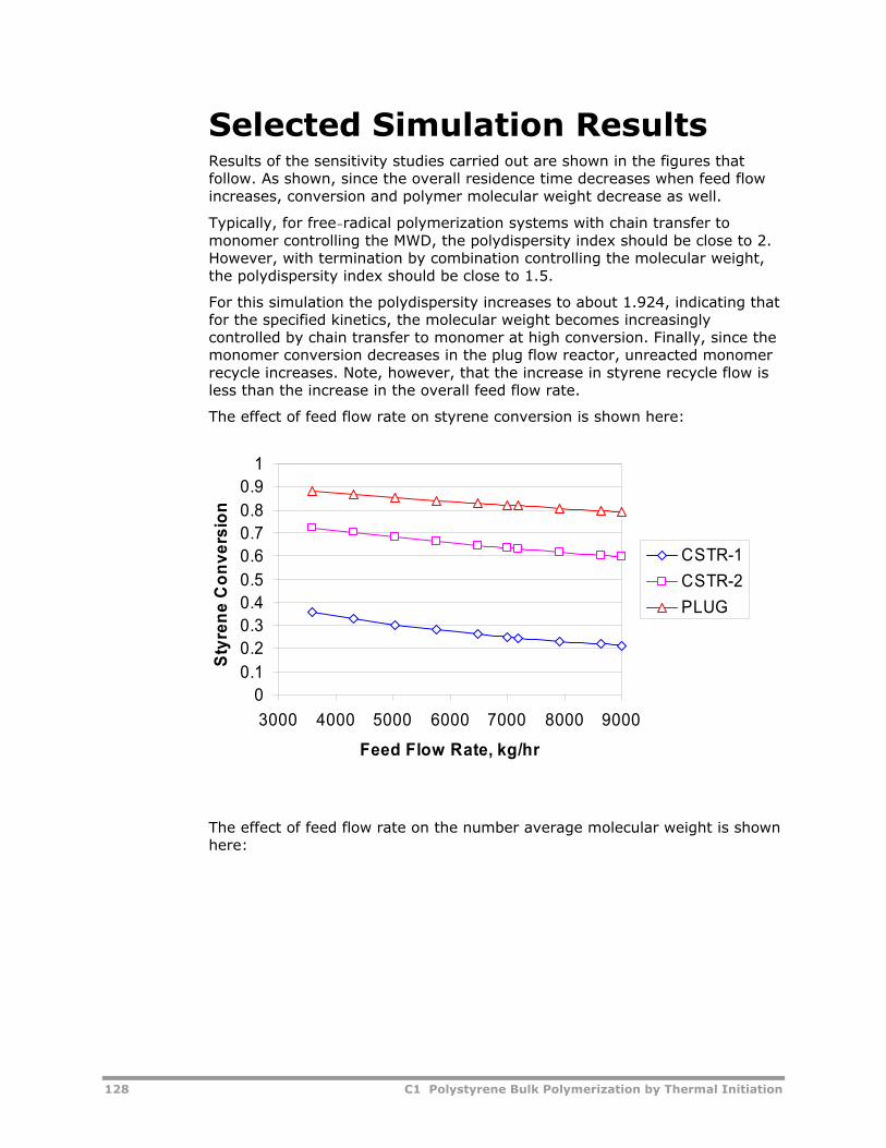
128 C1 Polystyrene Bulk Polymerization by Thermal Initiation
Selected Simulation Results Results of the sensitivity studies carried out are shown in the figures that follow. As shown, since the overall residence time decreases when feed flow increases, conversion and polymer molecular weight decrease as well.
Typically, for free-radical polymerization systems with chain transfer to monomer controlling the MWD, the polydispersity index should be close to 2. However, with termination by combination controlling the molecular weight, the polydispersity index should be close to 1.5.
For this simulation the polydispersity increases to about 1.924, indicating that for the specified kinetics, the molecular weight becomes increasingly controlled by chain transfer to monomer at high conversion. Finally, since the monomer conversion decreases in the plug flow reactor, unreacted monomer recycle increases. Note, however, that the increase in styrene recycle flow is less than the increase in the overall feed flow rate.
The effect of feed flow rate on styrene conversion is shown here:
00.10.20.30.40.50.60.70.80.9
1
3000 4000 5000 6000 7000 8000 9000
Feed Flow Rate, kg/hr
Styr
ene
Con
vers
ion
CSTR-1CSTR-2PLUG
The effect of feed flow rate on the number average molecular weight is shown here:
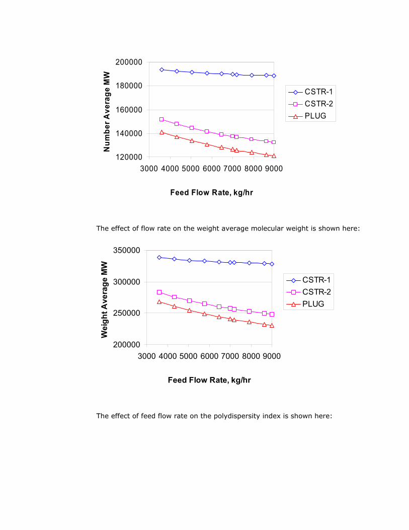
120000
140000
160000
180000
200000
3000 4000 5000 6000 7000 8000 9000
Feed Flow Rate, kg/hr
Num
ber A
vera
ge M
W
CSTR-1CSTR-2PLUG
The effect of flow rate on the weight average molecular weight is shown here:
200000
250000
300000
350000
3000 4000 5000 6000 7000 8000 9000
Feed Flow Rate, kg/hr
Wei
ght A
vera
ge M
W
CSTR-1CSTR-2PLUG
The effect of feed flow rate on the polydispersity index is shown here:
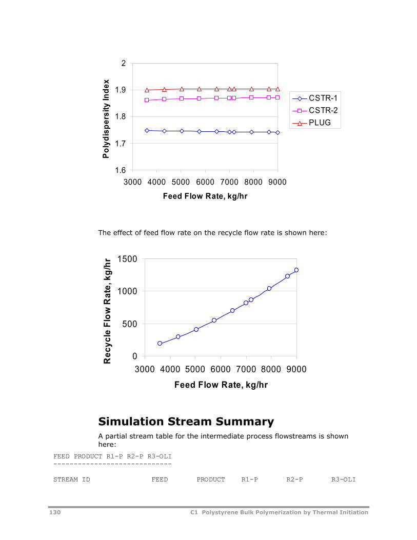
130 C1 Polystyrene Bulk Polymerization by Thermal Initiation
1.6
1.7
1.8
1.9
2
3000 4000 5000 6000 7000 8000 9000
Feed Flow Rate, kg/hr
Poly
disp
ersi
ty In
dex
CSTR-1CSTR-2PLUG
The effect of feed flow rate on the recycle flow rate is shown here:
0
500
1000
1500
3000 4000 5000 6000 7000 8000 9000
Feed Flow Rate, kg/hr
Rec
ycle
Flo
w R
ate,
kg/
hr
Simulation Stream Summary A partial stream table for the intermediate process flowstreams is shown here:
FEED PRODUCT R1-P R2-P R3-OLI ----------------------------- STREAM ID FEED PRODUCT R1-P R2-P R3-OLI
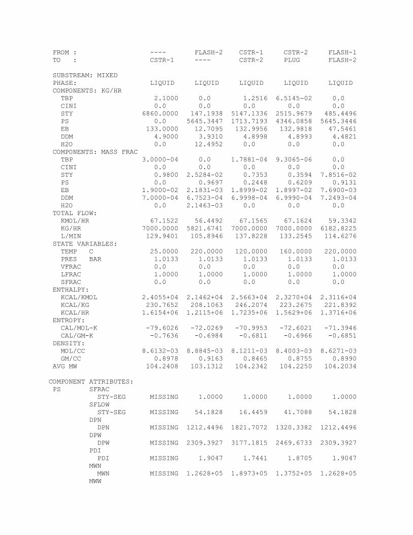
FROM : ---- FLASH-2 CSTR-1 CSTR-2 FLASH-1 TO : CSTR-1 ---- CSTR-2 PLUG FLASH-2 SUBSTREAM: MIXED PHASE: LIQUID LIQUID LIQUID LIQUID LIQUID COMPONENTS: KG/HR TBP 2.1000 0.0 1.2516 6.5145-02 0.0 CINI 0.0 0.0 0.0 0.0 0.0 STY 6860.0000 147.1938 5147.1336 2515.9679 485.4496 PS 0.0 5645.3447 1713.7193 4346.0858 5645.3446 EB 133.0000 12.7095 132.9956 132.9818 47.5461 DDM 4.9000 3.9310 4.8998 4.8993 4.4821 H2O 0.0 12.4952 0.0 0.0 0.0 COMPONENTS: MASS FRAC TBP 3.0000-04 0.0 1.7881-04 9.3065-06 0.0 CINI 0.0 0.0 0.0 0.0 0.0 STY 0.9800 2.5284-02 0.7353 0.3594 7.8516-02 PS 0.0 0.9697 0.2448 0.6209 0.9131 EB 1.9000-02 2.1831-03 1.8999-02 1.8997-02 7.6900-03 DDM 7.0000-04 6.7523-04 6.9998-04 6.9990-04 7.2493-04 H2O 0.0 2.1463-03 0.0 0.0 0.0 TOTAL FLOW: KMOL/HR 67.1522 56.4492 67.1565 67.1624 59.3342 KG/HR 7000.0000 5821.6741 7000.0000 7000.0000 6182.8225 L/MIN 129.9401 105.8946 137.8228 133.2545 114.6276 STATE VARIABLES: TEMP C 25.0000 220.0000 120.0000 160.0000 220.0000 PRES BAR 1.0133 1.0133 1.0133 1.0133 1.0133 VFRAC 0.0 0.0 0.0 0.0 0.0 LFRAC 1.0000 1.0000 1.0000 1.0000 1.0000 SFRAC 0.0 0.0 0.0 0.0 0.0 ENTHALPY: KCAL/KMOL 2.4055+04 2.1462+04 2.5663+04 2.3270+04 2.3116+04 KCAL/KG 230.7652 208.1063 246.2074 223.2675 221.8392 KCAL/HR 1.6154+06 1.2115+06 1.7235+06 1.5629+06 1.3716+06 ENTROPY: CAL/MOL-K -79.6026 -72.0269 -70.9953 -72.6021 -71.3946 CAL/GM-K -0.7636 -0.6984 -0.6811 -0.6966 -0.6851 DENSITY: MOL/CC 8.6132-03 8.8845-03 8.1211-03 8.4003-03 8.6271-03 GM/CC 0.8978 0.9163 0.8465 0.8755 0.8990 AVG MW 104.2408 103.1312 104.2342 104.2250 104.2034 COMPONENT ATTRIBUTES: PS SFRAC STY-SEG MISSING 1.0000 1.0000 1.0000 1.0000 SFLOW STY-SEG MISSING 54.1828 16.4459 41.7088 54.1828 DPN DPN MISSING 1212.4496 1821.7072 1320.3382 1212.4496 DPW DPW MISSING 2309.3927 3177.1815 2469.6733 2309.3927 PDI PDI MISSING 1.9047 1.7441 1.8705 1.9047 MWN MWN MISSING 1.2628+05 1.8973+05 1.3752+05 1.2628+05 MWW

132 C1 Polystyrene Bulk Polymerization by Thermal Initiation
MWW MISSING 2.4053+05 3.3091+05 2.5722+05 2.4053+05 ZMOM ZMOM MISSING 4.4689-02 9.0277-03 3.1589-02 4.4689-02 FMOM FMOM MISSING 54.1828 16.4459 41.7088 54.1828 SMOM SMOM MISSING 1.2513+05 5.2252+04 1.0301+05 1.2513+05 LDPN LDPN MISSING 568.1677 1170.7394 761.3834 568.1677 LZMOM LZMOM MISSING 2.9792-07 2.5496-07 3.2470-07 2.9792-07 LFMOM LFMOM MISSING 1.6927-04 2.9850-04 2.4722-04 1.6927-04 LSFLOW STY-SEG MISSING 1.6927-04 2.9850-04 2.4722-04 1.6927-04 LSFRAC STY-SEG MISSING 1.0000 1.0000 1.0000 1.0000 LEFLOW STY-SEG MISSING 2.9792-07 2.5496-07 3.2470-07 2.9792-07 LEFRAC STY-SEG MISSING 1.0000 1.0000 1.0000 1.0000 LPFRAC LPFRAC MISSING 6.6666-06 2.8242-05 1.0279-05 6.6666-06
References Albright, L.F. (1985). Processes for Major Addition-Type Plastics and Their Monomers. Krieger Publishing Co.
Brandrup, J., & Immergut, E. H. (1989). Polymer Handbook, 3rd Ed. Wiley Intersciences, 57-82.
Friis, N., & Hamielec, A. E. (1976). Gel-Effect in Emulsion Polymerization of Vinyl Monomers. ACS Symp. Ser., 24.
Gaur, U., & Wunderlich, B. (1982). J. Phys. Chem. Ref. Data, 11, (2), p. 313.
Hui, A. W., & Hamielec, A. E. (1972). Thermal Polymerization of Styrene at High Conversions and Temperatures. An Experimental Study. J. of Applied Polymer Science, 16, pp. 9-769.
Van Krevelen, D. W. (1990). Properties of Polymers, Their Correlation With Chemical Structure; Their Numerical Estimation and Prediction from Additive Group Contributions. New York: Elsevier.
Van Krevelen, D. W. (1990). Properties of Polymers, 3rd Ed., Amsterdam: Elsevier.
C2 Polystyrene with Styrene Monomer Distillation
The polystyrene with styrene monomer distillation model illustrates the use of Aspen Polymers Plus to model and predict the extent of polymer formation during styrene distillation. The model examines the optimum level of inhibitor to minimize polymer formation.
About This Process Product from a styrene plant consists of 63% styrene, 32% ethyl benzene and small amounts of toluene and benzene. Styrene is purified in a series of distillation columns. During distillation styrene polymerization occurs and the extent of polymerization depends on the time and temperature. To reduce polymer formation inhibitor is commonly used in the feed. The amount of inhibitor needs to be optimized since too little will produce more polymer waste and too high concentration of inhibitor will be expensive. The purpose of this example is to find an optimum level of inhibitor needed to minimize polymer formation and to maximize the process profitability.
Process Definition The process consists of three columns in series:
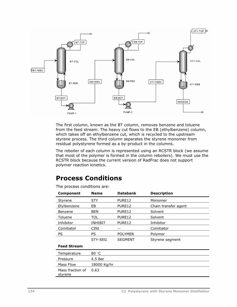
134 C2 Polystyrene with Styrene Monomer Distillation
The first column, known as the BT column, removes benzene and toluene from the feed stream. The heavy cut flows to the EB (ethylbenzene) column, which takes off an ethylbenzene cut, which is recycled to the upstream styrene process. The third column separates the styrene monomer from residual polystyrene formed as a by-product in the columns.
The reboiler of each column is represented using an RCSTR block (we assume that most of the polymer is formed in the column reboilers). We must use the RCSTR block because the current version of RadFrac does not support polymer reaction kinetics.
Process Conditions The process conditions are:
Component Name Databank Description
Styrene STY PURE12 Monomer
Etylbenzene EB PURE12 Chain transfer agent
Benzene BEN PURE12 Solvent
Toluene TOL PURE12 Solvent
Inhibitor INHIBIT PURE12 Inhibitor
Coinitiator CINI -- Coinitiator
PS PS POLYMER Polymer
STY-SEG SEGMENT Styrene segment
Feed Stream
Temperature 80 °C
Pressure 4.5 Bar
Mass Flow 18000 Kg/hr
Mass fraction of styrene
0.63

Mass fraction of ethyl benzene
0.318
Mass fraction of toluene
0.032
Mass fraction of benzene
0.02
Mass fraction of inhibitor
0.00
Operating Conditions
Block Temp (C)
Pres (Bar) Top/Bottom
Specifications
BT-COL 0.24 / 0.4 30 ideal stages + condenser
RR = 6.5
Feed - stage 20
BT-REB 109 0.4 Liquid holdup 22.5 m3
EB-COL 0.055 / 0.36 60 ideal stages + condenser
RR = 10
Feed - stage 33
EB-REB 113 0.36 Liquid holdup 18.5 m3
STY-COL 0.05 / 0.092 10 ideal stages + condenser
RR = 2.7
Feed - stage 2
STY-REB 100 0.092 Liquid holup 15 m3
Polymers and Segments Polystyrene is a homopolymer and the styrene segment is the only repeat unit. The set of component attributes required for free-radical polymerization is used for PS.
Physical Property Models and Data The Polymer Non-Random Two Liquid activity coefficient model (POLYNRTL) is used as the physical property method. Binary parameters for monomer/monomer pairs are drawn from Aspen’s binary databases. The monomer/styrene segment parameters are set equal to the equivalent parameters for monomer/sytrene pairs.
The thermophysical properties (density, heat capacity, etc.) of styrene, ethyl benzene, benzene, toluene and inhibitor are obtained from the Aspen Plus Pure Component Databank. Note that inhibitors are given the properties of styrene with the exception of molecular weight. The polymer thermophysical properties are calculated using the Van Krevelen group contribution method.
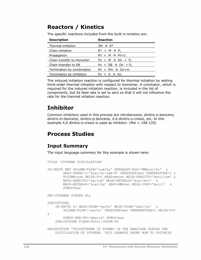
136 C2 Polystyrene with Styrene Monomer Distillation
Reactors / Kinetics The specific reactions included from the built-in kinetics are:
Description Reaction
Thermal initiation 3M R*
Chain initiation R* + M P1
Propagation Pn + M Pn+1
Chain transfer to monomer Pn + M Dn + P1
Chain thansfer to EB Pn + EB Dn + P1
Termination by combination Pn + Pm Dn+m
Termination by inhibition Pn + X Dn
The induced initiation reaction is configured for thermal initiation by setting third-order thermal initiation with respect to monomer. A coinitiator, which is required for the induced initiation reaction, is included in the list of components, but its feed rate is set to zero so that it will not influence the rate for the thermal initation reaction.
Inhibitor Common inhibitors used in this process are nitrobenzene, dinitro-o-bencene, dinitro-m-bencene, dinitro-p-bencene, 4,6 dinitro-o-cresol, etc. In this example 4,6 dinitro-o-cresol is used as inhibitor. (Mw = 198.135)
Process Studies
Input Summary The input language summary for this example is shown here:
TITLE 'STYRENE DISTILLATION' IN-UNITS MET VOLUME-FLOW='cum/hr' ENTHALPY-FLO='MMkcal/hr' & HEAT-TRANS-C='kcal/hr-sqm-K' PRESSURE=bar TEMPERATURE=C & VOLUME=cum DELTA-T=C HEAD=meter MOLE-DENSITY='kmol/cum' & MASS-DENSITY='kg/cum' MOLE-ENTHALP='kcal/mol' & MASS-ENTHALP='kcal/kg' HEAT=MMkcal MOLE-CONC='mol/l' & PDROP=bar DEF-STREAMS CONVEN ALL SIM-OPTIONS IN-UNITS SI MASS-FLOW='kg/hr' MOLE-FLOW='kmol/hr' & VOLUME-FLOW='cum/hr' PRESSURE=bar TEMPERATURE=C DELTA-T=C & PDROP-PER-HT='mbar/m' PDROP=bar SIM-OPTIONS FLASH-TOL=1.0000E-06 DESCRIPTION “POLYSTYRENE IS FORMED IN THE REBOILER DURING THE DISTILLATION OF STYRENE. THIS EXAMPLE SHOWS HOW TO OPTIMIZE
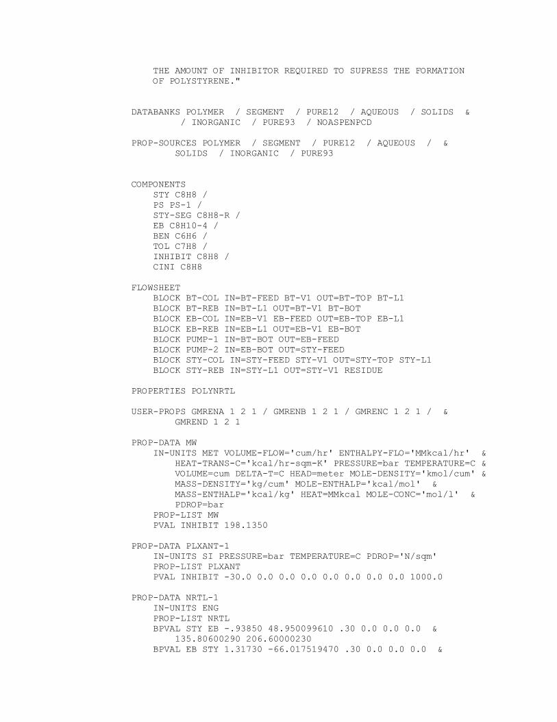
THE AMOUNT OF INHIBITOR REQUIRED TO SUPRESS THE FORMATION OF POLYSTYRENE." DATABANKS POLYMER / SEGMENT / PURE12 / AQUEOUS / SOLIDS & / INORGANIC / PURE93 / NOASPENPCD PROP-SOURCES POLYMER / SEGMENT / PURE12 / AQUEOUS / & SOLIDS / INORGANIC / PURE93 COMPONENTS STY C8H8 / PS PS-1 / STY-SEG C8H8-R / EB C8H10-4 / BEN C6H6 / TOL C7H8 / INHIBIT C8H8 / CINI C8H8 FLOWSHEET BLOCK BT-COL IN=BT-FEED BT-V1 OUT=BT-TOP BT-L1 BLOCK BT-REB IN=BT-L1 OUT=BT-V1 BT-BOT BLOCK EB-COL IN=EB-V1 EB-FEED OUT=EB-TOP EB-L1 BLOCK EB-REB IN=EB-L1 OUT=EB-V1 EB-BOT BLOCK PUMP-1 IN=BT-BOT OUT=EB-FEED BLOCK PUMP-2 IN=EB-BOT OUT=STY-FEED BLOCK STY-COL IN=STY-FEED STY-V1 OUT=STY-TOP STY-L1 BLOCK STY-REB IN=STY-L1 OUT=STY-V1 RESIDUE PROPERTIES POLYNRTL USER-PROPS GMRENA 1 2 1 / GMRENB 1 2 1 / GMRENC 1 2 1 / & GMREND 1 2 1 PROP-DATA MW IN-UNITS MET VOLUME-FLOW='cum/hr' ENTHALPY-FLO='MMkcal/hr' & HEAT-TRANS-C='kcal/hr-sqm-K' PRESSURE=bar TEMPERATURE=C & VOLUME=cum DELTA-T=C HEAD=meter MOLE-DENSITY='kmol/cum' & MASS-DENSITY='kg/cum' MOLE-ENTHALP='kcal/mol' & MASS-ENTHALP='kcal/kg' HEAT=MMkcal MOLE-CONC='mol/l' & PDROP=bar PROP-LIST MW PVAL INHIBIT 198.1350 PROP-DATA PLXANT-1 IN-UNITS SI PRESSURE=bar TEMPERATURE=C PDROP='N/sqm' PROP-LIST PLXANT PVAL INHIBIT -30.0 0.0 0.0 0.0 0.0 0.0 0.0 0.0 1000.0 PROP-DATA NRTL-1 IN-UNITS ENG PROP-LIST NRTL BPVAL STY EB -.93850 48.950099610 .30 0.0 0.0 0.0 & 135.80600290 206.60000230 BPVAL EB STY 1.31730 -66.017519470 .30 0.0 0.0 0.0 &
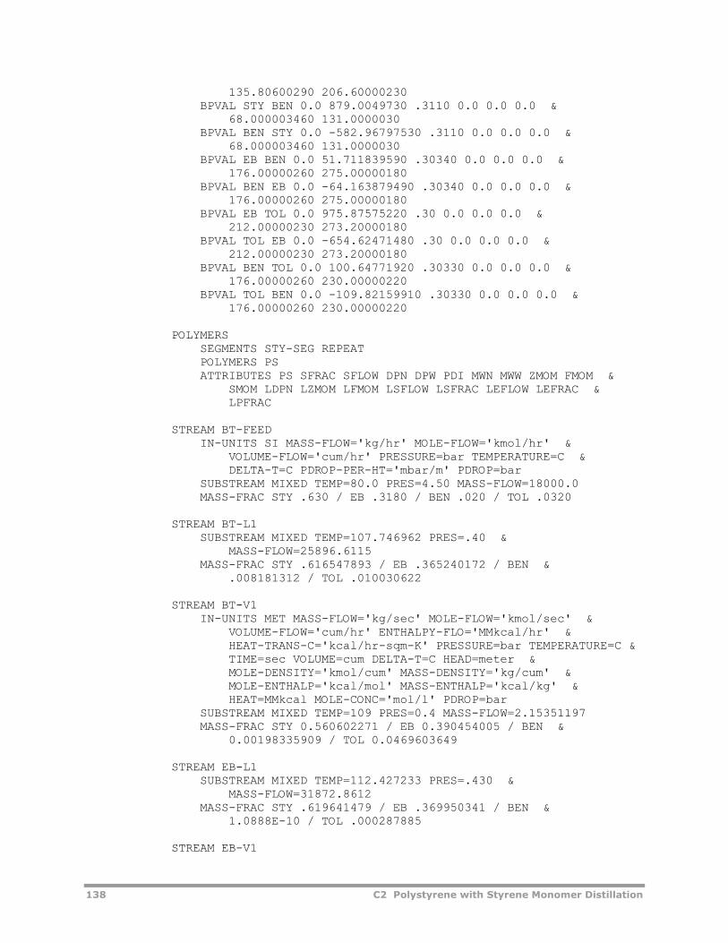
138 C2 Polystyrene with Styrene Monomer Distillation
135.80600290 206.60000230 BPVAL STY BEN 0.0 879.0049730 .3110 0.0 0.0 0.0 & 68.000003460 131.0000030 BPVAL BEN STY 0.0 -582.96797530 .3110 0.0 0.0 0.0 & 68.000003460 131.0000030 BPVAL EB BEN 0.0 51.711839590 .30340 0.0 0.0 0.0 & 176.00000260 275.00000180 BPVAL BEN EB 0.0 -64.163879490 .30340 0.0 0.0 0.0 & 176.00000260 275.00000180 BPVAL EB TOL 0.0 975.87575220 .30 0.0 0.0 0.0 & 212.00000230 273.20000180 BPVAL TOL EB 0.0 -654.62471480 .30 0.0 0.0 0.0 & 212.00000230 273.20000180 BPVAL BEN TOL 0.0 100.64771920 .30330 0.0 0.0 0.0 & 176.00000260 230.00000220 BPVAL TOL BEN 0.0 -109.82159910 .30330 0.0 0.0 0.0 & 176.00000260 230.00000220 POLYMERS SEGMENTS STY-SEG REPEAT POLYMERS PS ATTRIBUTES PS SFRAC SFLOW DPN DPW PDI MWN MWW ZMOM FMOM & SMOM LDPN LZMOM LFMOM LSFLOW LSFRAC LEFLOW LEFRAC & LPFRAC STREAM BT-FEED IN-UNITS SI MASS-FLOW='kg/hr' MOLE-FLOW='kmol/hr' & VOLUME-FLOW='cum/hr' PRESSURE=bar TEMPERATURE=C & DELTA-T=C PDROP-PER-HT='mbar/m' PDROP=bar SUBSTREAM MIXED TEMP=80.0 PRES=4.50 MASS-FLOW=18000.0 MASS-FRAC STY .630 / EB .3180 / BEN .020 / TOL .0320 STREAM BT-L1 SUBSTREAM MIXED TEMP=107.746962 PRES=.40 & MASS-FLOW=25896.6115 MASS-FRAC STY .616547893 / EB .365240172 / BEN & .008181312 / TOL .010030622 STREAM BT-V1 IN-UNITS MET MASS-FLOW='kg/sec' MOLE-FLOW='kmol/sec' & VOLUME-FLOW='cum/hr' ENTHALPY-FLO='MMkcal/hr' & HEAT-TRANS-C='kcal/hr-sqm-K' PRESSURE=bar TEMPERATURE=C & TIME=sec VOLUME=cum DELTA-T=C HEAD=meter & MOLE-DENSITY='kmol/cum' MASS-DENSITY='kg/cum' & MOLE-ENTHALP='kcal/mol' MASS-ENTHALP='kcal/kg' & HEAT=MMkcal MOLE-CONC='mol/l' PDROP=bar SUBSTREAM MIXED TEMP=109 PRES=0.4 MASS-FLOW=2.15351197 MASS-FRAC STY 0.560602271 / EB 0.390454005 / BEN & 0.00198335909 / TOL 0.0469603649 STREAM EB-L1 SUBSTREAM MIXED TEMP=112.427233 PRES=.430 & MASS-FLOW=31872.8612 MASS-FRAC STY .619641479 / EB .369950341 / BEN & 1.0888E-10 / TOL .000287885 STREAM EB-V1
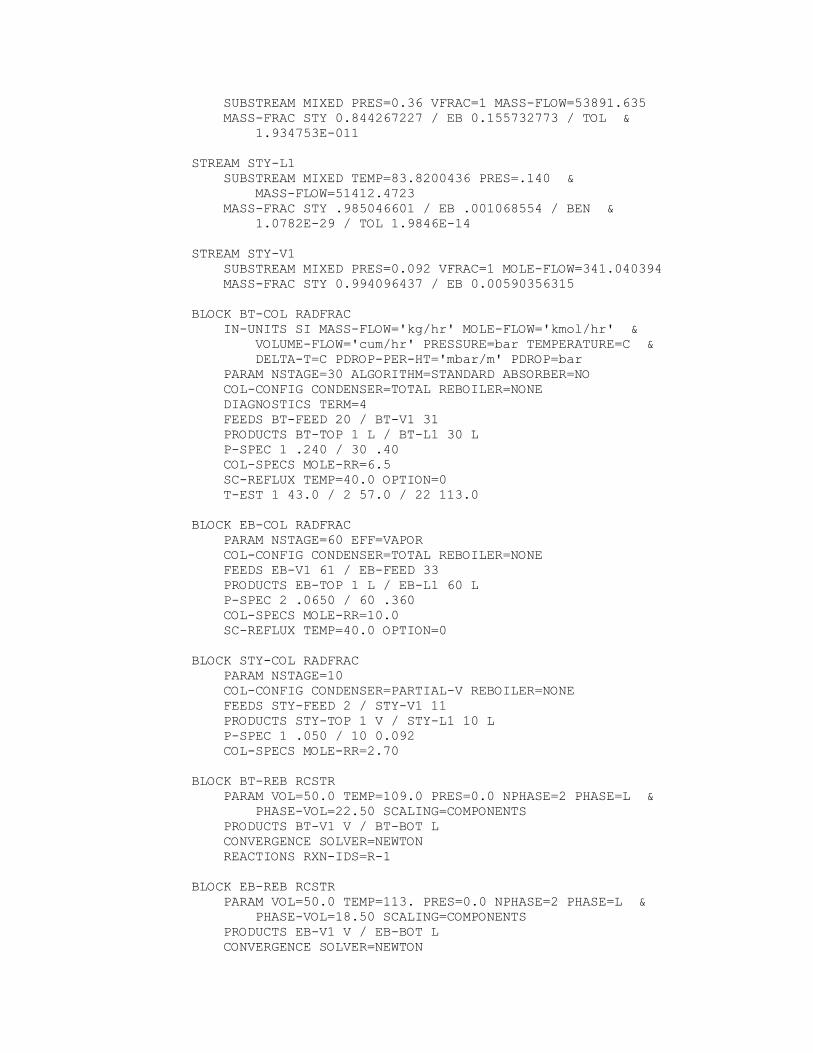
SUBSTREAM MIXED PRES=0.36 VFRAC=1 MASS-FLOW=53891.635 MASS-FRAC STY 0.844267227 / EB 0.155732773 / TOL & 1.934753E-011 STREAM STY-L1 SUBSTREAM MIXED TEMP=83.8200436 PRES=.140 & MASS-FLOW=51412.4723 MASS-FRAC STY .985046601 / EB .001068554 / BEN & 1.0782E-29 / TOL 1.9846E-14 STREAM STY-V1 SUBSTREAM MIXED PRES=0.092 VFRAC=1 MOLE-FLOW=341.040394 MASS-FRAC STY 0.994096437 / EB 0.00590356315 BLOCK BT-COL RADFRAC IN-UNITS SI MASS-FLOW='kg/hr' MOLE-FLOW='kmol/hr' & VOLUME-FLOW='cum/hr' PRESSURE=bar TEMPERATURE=C & DELTA-T=C PDROP-PER-HT='mbar/m' PDROP=bar PARAM NSTAGE=30 ALGORITHM=STANDARD ABSORBER=NO COL-CONFIG CONDENSER=TOTAL REBOILER=NONE DIAGNOSTICS TERM=4 FEEDS BT-FEED 20 / BT-V1 31 PRODUCTS BT-TOP 1 L / BT-L1 30 L P-SPEC 1 .240 / 30 .40 COL-SPECS MOLE-RR=6.5 SC-REFLUX TEMP=40.0 OPTION=0 T-EST 1 43.0 / 2 57.0 / 22 113.0 BLOCK EB-COL RADFRAC PARAM NSTAGE=60 EFF=VAPOR COL-CONFIG CONDENSER=TOTAL REBOILER=NONE FEEDS EB-V1 61 / EB-FEED 33 PRODUCTS EB-TOP 1 L / EB-L1 60 L P-SPEC 2 .0650 / 60 .360 COL-SPECS MOLE-RR=10.0 SC-REFLUX TEMP=40.0 OPTION=0 BLOCK STY-COL RADFRAC PARAM NSTAGE=10 COL-CONFIG CONDENSER=PARTIAL-V REBOILER=NONE FEEDS STY-FEED 2 / STY-V1 11 PRODUCTS STY-TOP 1 V / STY-L1 10 L P-SPEC 1 .050 / 10 0.092 COL-SPECS MOLE-RR=2.70 BLOCK BT-REB RCSTR PARAM VOL=50.0 TEMP=109.0 PRES=0.0 NPHASE=2 PHASE=L & PHASE-VOL=22.50 SCALING=COMPONENTS PRODUCTS BT-V1 V / BT-BOT L CONVERGENCE SOLVER=NEWTON REACTIONS RXN-IDS=R-1 BLOCK EB-REB RCSTR PARAM VOL=50.0 TEMP=113. PRES=0.0 NPHASE=2 PHASE=L & PHASE-VOL=18.50 SCALING=COMPONENTS PRODUCTS EB-V1 V / EB-BOT L CONVERGENCE SOLVER=NEWTON
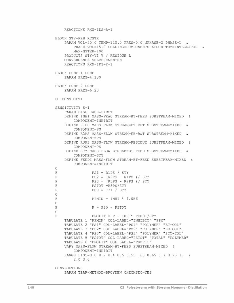
140 C2 Polystyrene with Styrene Monomer Distillation
REACTIONS RXN-IDS=R-1 BLOCK STY-REB RCSTR PARAM VOL=50.0 TEMP=120.0 PRES=0.0 NPHASE=2 PHASE=L & PHASE-VOL=15.0 SCALING=COMPONENTS ALGORITHM=INTEGRATOR & MAX-NSTEP=100 PRODUCTS STY-V1 V / RESIDUE L CONVERGENCE SOLVER=NEWTON REACTIONS RXN-IDS=R-1 BLOCK PUMP-1 PUMP PARAM PRES=4.130 BLOCK PUMP-2 PUMP PARAM PRES=6.20 EO-CONV-OPTI SENSITIVITY S-1 PARAM BASE-CASE=FIRST DEFINE INHI MASS-FRAC STREAM=BT-FEED SUBSTREAM=MIXED & COMPONENT=INHIBIT DEFINE R1PS MASS-FLOW STREAM=BT-BOT SUBSTREAM=MIXED & COMPONENT=PS DEFINE R2PS MASS-FLOW STREAM=EB-BOT SUBSTREAM=MIXED & COMPONENT=PS DEFINE R3PS MASS-FLOW STREAM=RESIDUE SUBSTREAM=MIXED & COMPONENT=PS DEFINE STY MASS-FLOW STREAM=BT-FEED SUBSTREAM=MIXED & COMPONENT=STY DEFINE FEEDI MASS-FLOW STREAM=BT-FEED SUBSTREAM=MIXED & COMPONENT=INHIBIT C F PS1 = R1PS / STY F PS2 = (R2PS - R1PS )/ STY F PS3 = (R3PS - R2PS )/ STY F PSTOT =R3PS/STY F PS0 = 731 / STY C F PPMIN = INHI * 1.0E6 C F P = PS0 - PSTOT C F PROFIT = P - 100 * FEEDI/STY TABULATE 1 "PPMIN" COL-LABEL="INHIBIT" "PPM" TABULATE 2 "PS1" COL-LABEL="PS1" "POLYMER" "BT-COL" TABULATE 3 "PS2" COL-LABEL="PS2" "POLYMER" "EB-COL" TABULATE 4 "PS3" COL-LABEL="PS3" "POLYMER" "STY-COL" TABULATE 5 "PSTOT" COL-LABEL="PSTOT" "TOTAL" "POLYMER" TABULATE 6 "PROFIT" COL-LABEL="PROFIT" VARY MASS-FLOW STREAM=BT-FEED SUBSTREAM=MIXED & COMPONENT=INHIBIT RANGE LIST=0.0 0.2 0.4 0.5 0.55 .60 0.65 0.7 0.75 1. & 2.0 3.0 CONV-OPTIONS PARAM TEAR-METHOD=BROYDEN CHECKSEQ=YES
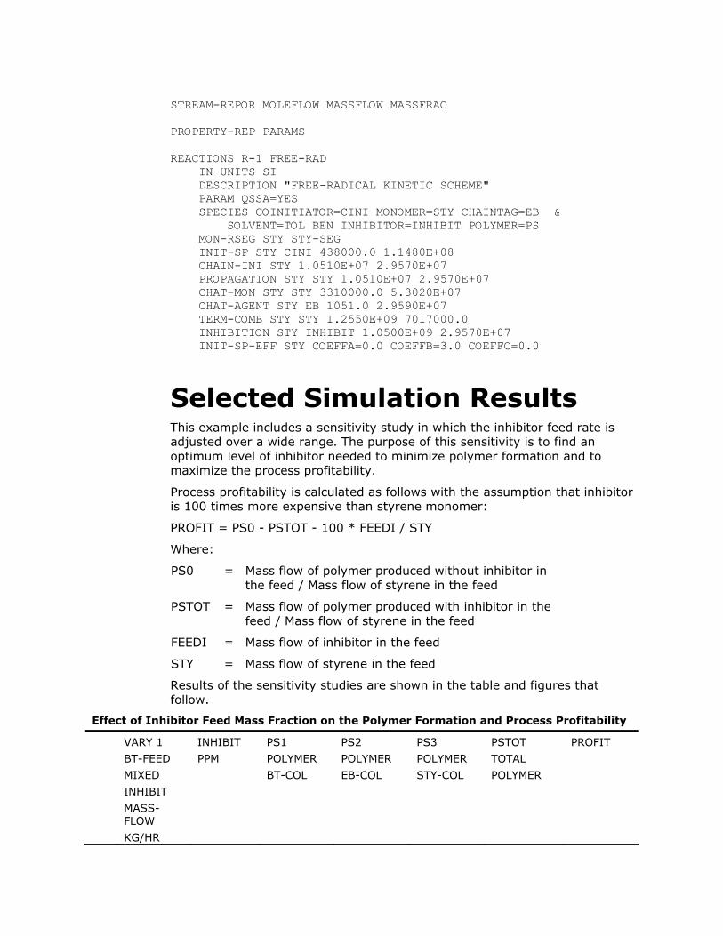
STREAM-REPOR MOLEFLOW MASSFLOW MASSFRAC PROPERTY-REP PARAMS REACTIONS R-1 FREE-RAD IN-UNITS SI DESCRIPTION "FREE-RADICAL KINETIC SCHEME" PARAM QSSA=YES SPECIES COINITIATOR=CINI MONOMER=STY CHAINTAG=EB & SOLVENT=TOL BEN INHIBITOR=INHIBIT POLYMER=PS MON-RSEG STY STY-SEG INIT-SP STY CINI 438000.0 1.1480E+08 CHAIN-INI STY 1.0510E+07 2.9570E+07 PROPAGATION STY STY 1.0510E+07 2.9570E+07 CHAT-MON STY STY 3310000.0 5.3020E+07 CHAT-AGENT STY EB 1051.0 2.9590E+07 TERM-COMB STY STY 1.2550E+09 7017000.0 INHIBITION STY INHIBIT 1.0500E+09 2.9570E+07 INIT-SP-EFF STY COEFFA=0.0 COEFFB=3.0 COEFFC=0.0
Selected Simulation Results This example includes a sensitivity study in which the inhibitor feed rate is adjusted over a wide range. The purpose of this sensitivity is to find an optimum level of inhibitor needed to minimize polymer formation and to maximize the process profitability.
Process profitability is calculated as follows with the assumption that inhibitor is 100 times more expensive than styrene monomer:
PROFIT = PS0 - PSTOT - 100 * FEEDI / STY
Where:
PS0 = Mass flow of polymer produced without inhibitor in the feed / Mass flow of styrene in the feed
PSTOT = Mass flow of polymer produced with inhibitor in the feed / Mass flow of styrene in the feed
FEEDI = Mass flow of inhibitor in the feed
STY = Mass flow of styrene in the feed
Results of the sensitivity studies are shown in the table and figures that follow.
Effect of Inhibitor Feed Mass Fraction on the Polymer Formation and Process Profitability
VARY 1
BT-FEED
MIXED
INHIBIT
MASS-FLOW
KG/HR
INHIBIT
PPM
PS1
POLYMER
BT-COL
PS2
POLYMER
EB-COL
PS3
POLYMER
STY-COL
PSTOT
TOTAL
POLYMER
PROFIT
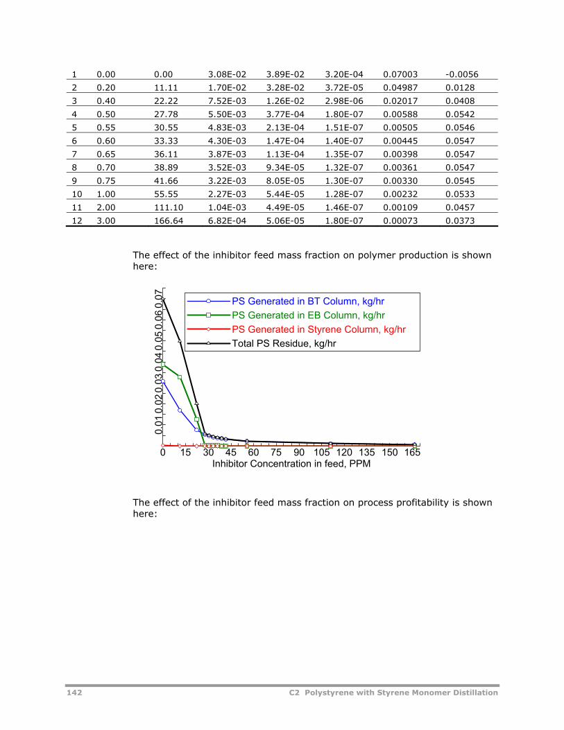
142 C2 Polystyrene with Styrene Monomer Distillation
1 0.00 0.00 3.08E-02 3.89E-02 3.20E-04 0.07003 -0.0056
2 0.20 11.11 1.70E-02 3.28E-02 3.72E-05 0.04987 0.0128
3 0.40 22.22 7.52E-03 1.26E-02 2.98E-06 0.02017 0.0408
4 0.50 27.78 5.50E-03 3.77E-04 1.80E-07 0.00588 0.0542
5 0.55 30.55 4.83E-03 2.13E-04 1.51E-07 0.00505 0.0546
6 0.60 33.33 4.30E-03 1.47E-04 1.40E-07 0.00445 0.0547
7 0.65 36.11 3.87E-03 1.13E-04 1.35E-07 0.00398 0.0547
8 0.70 38.89 3.52E-03 9.34E-05 1.32E-07 0.00361 0.0547
9 0.75 41.66 3.22E-03 8.05E-05 1.30E-07 0.00330 0.0545
10 1.00 55.55 2.27E-03 5.44E-05 1.28E-07 0.00232 0.0533
11 2.00 111.10 1.04E-03 4.49E-05 1.46E-07 0.00109 0.0457
12 3.00 166.64 6.82E-04 5.06E-05 1.80E-07 0.00073 0.0373
The effect of the inhibitor feed mass fraction on polymer production is shown here:
Inhibitor Concentration in feed, PPM
0 15 30 45 60 75 90 105 120 135 150 165
0.01
0.02
0.03
0.04
0.05
0.06
0.07 PS Generated in BT Column, kg/hr
PS Generated in EB Column, kg/hrPS Generated in Styrene Column, kg/hr Total PS Residue, kg/hr
The effect of the inhibitor feed mass fraction on process profitability is shown here:
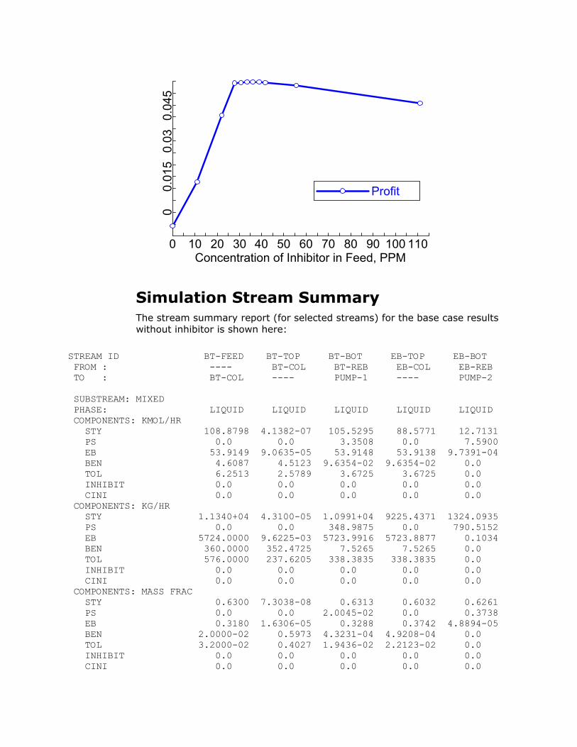
Concentration of Inhibitor in Feed, PPM
0 10 20 30 40 50 60 70 80 90 100 110
00.
015
0.03
0.04
5
Profit
Simulation Stream Summary The stream summary report (for selected streams) for the base case results without inhibitor is shown here:
STREAM ID BT-FEED BT-TOP BT-BOT EB-TOP EB-BOT FROM : ---- BT-COL BT-REB EB-COL EB-REB TO : BT-COL ---- PUMP-1 ---- PUMP-2 SUBSTREAM: MIXED PHASE: LIQUID LIQUID LIQUID LIQUID LIQUID COMPONENTS: KMOL/HR STY 108.8798 4.1382-07 105.5295 88.5771 12.7131 PS 0.0 0.0 3.3508 0.0 7.5900 EB 53.9149 9.0635-05 53.9148 53.9138 9.7391-04 BEN 4.6087 4.5123 9.6354-02 9.6354-02 0.0 TOL 6.2513 2.5789 3.6725 3.6725 0.0 INHIBIT 0.0 0.0 0.0 0.0 0.0 CINI 0.0 0.0 0.0 0.0 0.0 COMPONENTS: KG/HR STY 1.1340+04 4.3100-05 1.0991+04 9225.4371 1324.0935 PS 0.0 0.0 348.9875 0.0 790.5152 EB 5724.0000 9.6225-03 5723.9916 5723.8877 0.1034 BEN 360.0000 352.4725 7.5265 7.5265 0.0 TOL 576.0000 237.6205 338.3835 338.3835 0.0 INHIBIT 0.0 0.0 0.0 0.0 0.0 CINI 0.0 0.0 0.0 0.0 0.0 COMPONENTS: MASS FRAC STY 0.6300 7.3038-08 0.6313 0.6032 0.6261 PS 0.0 0.0 2.0045-02 0.0 0.3738 EB 0.3180 1.6306-05 0.3288 0.3742 4.8894-05 BEN 2.0000-02 0.5973 4.3231-04 4.9208-04 0.0 TOL 3.2000-02 0.4027 1.9436-02 2.2123-02 0.0 INHIBIT 0.0 0.0 0.0 0.0 0.0 CINI 0.0 0.0 0.0 0.0 0.0
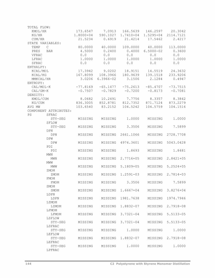
144 C2 Polystyrene with Styrene Monomer Distillation
TOTAL FLOW: KMOL/HR 173.6547 7.0913 166.5639 146.2597 20.3042 KG/HR 1.8000+04 590.1027 1.7410+04 1.5295+04 2114.7121 CUM/HR 21.5234 0.6919 21.4214 17.5462 2.4217 STATE VARIABLES: TEMP C 80.0000 40.0000 109.0000 40.0000 113.0000 PRES BAR 4.5000 0.2400 0.4000 6.5000-02 0.3600 VFRAC 0.0 0.0 0.0 0.0 0.0 LFRAC 1.0000 1.0000 1.0000 1.0000 1.0000 SFRAC 0.0 0.0 0.0 0.0 0.0 ENTHALPY: KCAL/MOL 17.3942 9.0202 18.9151 14.5519 24.3632 KCAL/KG 167.8099 108.3966 180.9639 139.1518 233.9206 MMKCAL/HR 3.0206 6.3966-02 3.1506 2.1284 0.4947 ENTROPY: CAL/MOL-K -77.8169 -65.1477 -75.2613 -85.4707 -73.7515 CAL/GM-K -0.7507 -0.7829 -0.7200 -0.8173 -0.7081 DENSITY: KMOL/CUM 8.0682 10.2491 7.7756 8.3357 8.3842 KG/CUM 836.3005 852.8781 812.7352 871.7124 873.2279 AVG MW 103.6540 83.2152 104.5242 104.5759 104.1516 COMPONENT ATTRIBUTES: PS SFRAC STY-SEG MISSING MISSING 1.0000 MISSING 1.0000 SFLOW STY-SEG MISSING MISSING 3.3506 MISSING 7.5899 DPN DPN MISSING MISSING 2661.1066 MISSING 2728.7708 DPW DPW MISSING MISSING 4974.3601 MISSING 5043.0428 PDI PDI MISSING MISSING 1.8693 MISSING 1.8481 MWN MWN MISSING MISSING 2.7716+05 MISSING 2.8421+05 MWW MWW MISSING MISSING 5.1809+05 MISSING 5.2524+05 ZMOM ZMOM MISSING MISSING 1.2591-03 MISSING 2.7814-03 FMOM FMOM MISSING MISSING 3.3506 MISSING 7.5899 SMOM SMOM MISSING MISSING 1.6667+04 MISSING 3.8276+04 LDPN LDPN MISSING MISSING 1981.7638 MISSING 1974.7946 LZMOM LZMOM MISSING MISSING 1.8832-07 MISSING 2.7918-08 LFMOM LFMOM MISSING MISSING 3.7321-04 MISSING 5.5133-05 LSFLOW STY-SEG MISSING MISSING 3.7321-04 MISSING 5.5133-05 LSFRAC STY-SEG MISSING MISSING 1.0000 MISSING 1.0000 LEFLOW STY-SEG MISSING MISSING 1.8832-07 MISSING 2.7918-08 LEFRAC STY-SEG MISSING MISSING 1.0000 MISSING 1.0000 LPFRAC
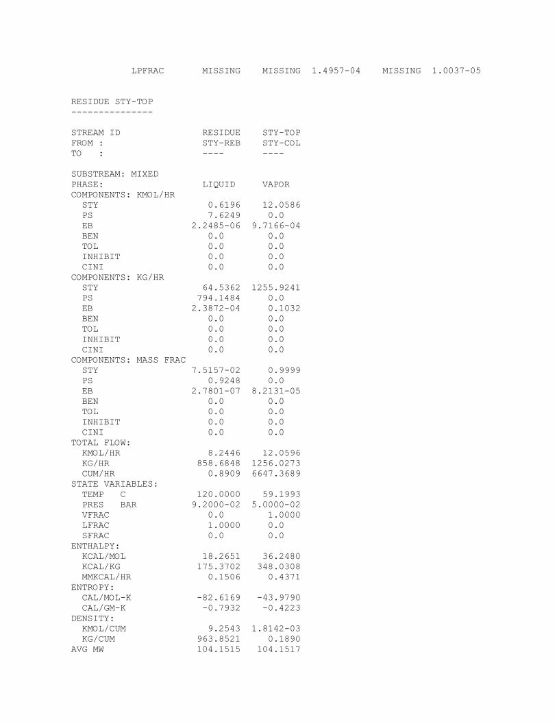
LPFRAC MISSING MISSING 1.4957-04 MISSING 1.0037-05 RESIDUE STY-TOP --------------- STREAM ID RESIDUE STY-TOP FROM : STY-REB STY-COL TO : ---- ---- SUBSTREAM: MIXED PHASE: LIQUID VAPOR COMPONENTS: KMOL/HR STY 0.6196 12.0586 PS 7.6249 0.0 EB 2.2485-06 9.7166-04 BEN 0.0 0.0 TOL 0.0 0.0 INHIBIT 0.0 0.0 CINI 0.0 0.0 COMPONENTS: KG/HR STY 64.5362 1255.9241 PS 794.1484 0.0 EB 2.3872-04 0.1032 BEN 0.0 0.0 TOL 0.0 0.0 INHIBIT 0.0 0.0 CINI 0.0 0.0 COMPONENTS: MASS FRAC STY 7.5157-02 0.9999 PS 0.9248 0.0 EB 2.7801-07 8.2131-05 BEN 0.0 0.0 TOL 0.0 0.0 INHIBIT 0.0 0.0 CINI 0.0 0.0 TOTAL FLOW: KMOL/HR 8.2446 12.0596 KG/HR 858.6848 1256.0273 CUM/HR 0.8909 6647.3689 STATE VARIABLES: TEMP C 120.0000 59.1993 PRES BAR 9.2000-02 5.0000-02 VFRAC 0.0 1.0000 LFRAC 1.0000 0.0 SFRAC 0.0 0.0 ENTHALPY: KCAL/MOL 18.2651 36.2480 KCAL/KG 175.3702 348.0308 MMKCAL/HR 0.1506 0.4371 ENTROPY: CAL/MOL-K -82.6169 -43.9790 CAL/GM-K -0.7932 -0.4223 DENSITY: KMOL/CUM 9.2543 1.8142-03 KG/CUM 963.8521 0.1890 AVG MW 104.1515 104.1517
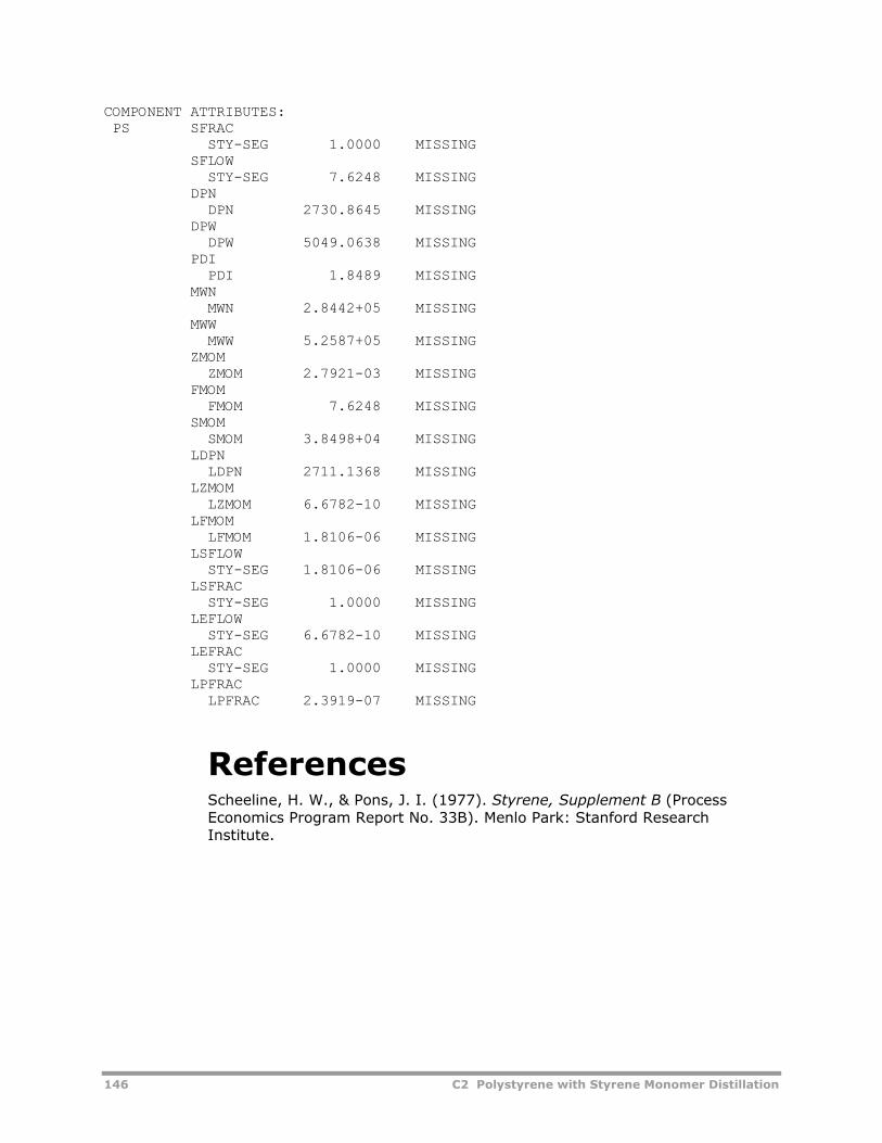
146 C2 Polystyrene with Styrene Monomer Distillation
COMPONENT ATTRIBUTES: PS SFRAC STY-SEG 1.0000 MISSING SFLOW STY-SEG 7.6248 MISSING DPN DPN 2730.8645 MISSING DPW DPW 5049.0638 MISSING PDI PDI 1.8489 MISSING MWN MWN 2.8442+05 MISSING MWW MWW 5.2587+05 MISSING ZMOM ZMOM 2.7921-03 MISSING FMOM FMOM 7.6248 MISSING SMOM SMOM 3.8498+04 MISSING LDPN LDPN 2711.1368 MISSING LZMOM LZMOM 6.6782-10 MISSING LFMOM LFMOM 1.8106-06 MISSING LSFLOW STY-SEG 1.8106-06 MISSING LSFRAC STY-SEG 1.0000 MISSING LEFLOW STY-SEG 6.6782-10 MISSING LEFRAC STY-SEG 1.0000 MISSING LPFRAC LPFRAC 2.3919-07 MISSING
References Scheeline, H. W., & Pons, J. I. (1977). Styrene, Supplement B (Process Economics Program Report No. 33B). Menlo Park: Stanford Research Institute.
C3 Expanded Polystyrene Suspension Polymerization
The expanded polystyrene (EPS) suspension polymerization model illustrates the use of Aspen Polymers Plus for modeling free-radical suspension polymerization of styrene in a batch reactor. The batch reactor model, RBatch, rigorously accounts for two liquid phases and one vapor phase. The reactions take place in the organic (monomer/polymer droplets) phase.
The first polymerization stage of the EPS process and the effect of n-pentane on the conversion and molecular weight profiles are studied. The results reproduce the published work of Villalobos and coworkers (1993). This application example also compares the use of monofunctional and bifunctional initiators. Note that Aspen Polymers Plus currently does not support bifunctional initiators.
About This Process The manufacture of expandable polystyrene involves two stages. During the first stage, suspension polymerization of styrene is carried out in a stirred batch reactor at temperatures between 80 and 90°C with a dispersed phase hold-up (volume of monomer phase over total liquid volume) in the range of 0.4 to 0.6.
Styrene monomer is suspended in the form of droplets in water phase. Polymerization occurs in these droplets until the mixture reaches its glass transition temperature. The mean particle size is determined by the droplet coalescence and the droplet breakage caused by the agitation system. The particle growth is controlled with the aid of suspending agents, which are usually inorganic powders such as tricalcium phosphate.
In the second stage, also known as the impregnation stage, a blowing agent, such as n-pentane, is loaded into the reactor and diffuses into the beads. The residual monomer is polymerized using an initiator with a half-life higher than the one used in the polymerization process. The batch reactor is operated at elevated pressures during this second, impregnation, stage.
A main manufacturing objective is to minimize the long batch times necessary to complete the polymerization. Polymerization at higher temperatures as a
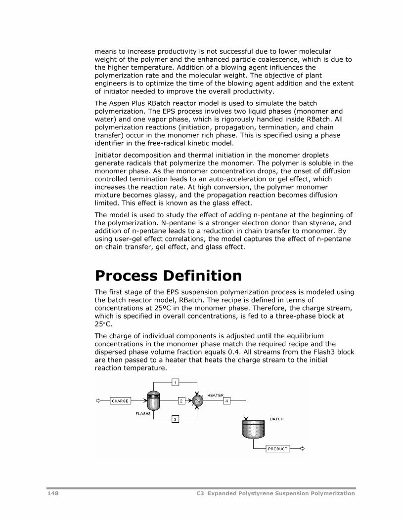
148 C3 Expanded Polystyrene Suspension Polymerization
means to increase productivity is not successful due to lower molecular weight of the polymer and the enhanced particle coalescence, which is due to the higher temperature. Addition of a blowing agent influences the polymerization rate and the molecular weight. The objective of plant engineers is to optimize the time of the blowing agent addition and the extent of initiator needed to improve the overall productivity.
The Aspen Plus RBatch reactor model is used to simulate the batch polymerization. The EPS process involves two liquid phases (monomer and water) and one vapor phase, which is rigorously handled inside RBatch. All polymerization reactions (initiation, propagation, termination, and chain transfer) occur in the monomer rich phase. This is specified using a phase identifier in the free-radical kinetic model.
Initiator decomposition and thermal initiation in the monomer droplets generate radicals that polymerize the monomer. The polymer is soluble in the monomer phase. As the monomer concentration drops, the onset of diffusion controlled termination leads to an auto-acceleration or gel effect, which increases the reaction rate. At high conversion, the polymer monomer mixture becomes glassy, and the propagation reaction becomes diffusion limited. This effect is known as the glass effect.
The model is used to study the effect of adding n-pentane at the beginning of the polymerization. N-pentane is a stronger electron donor than styrene, and addition of n-pentane leads to a reduction in chain transfer to monomer. By using user-gel effect correlations, the model captures the effect of n-pentane on chain transfer, gel effect, and glass effect.
Process Definition The first stage of the EPS suspension polymerization process is modeled using the batch reactor model, RBatch. The recipe is defined in terms of concentrations at 25ºC in the monomer phase. Therefore, the charge stream, which is specified in overall concentrations, is fed to a three-phase block at 25°C.
The charge of individual components is adjusted until the equilibrium concentrations in the monomer phase match the required recipe and the dispersed phase volume fraction equals 0.4. All streams from the Flash3 block are then passed to a heater that heats the charge stream to the initial reaction temperature.
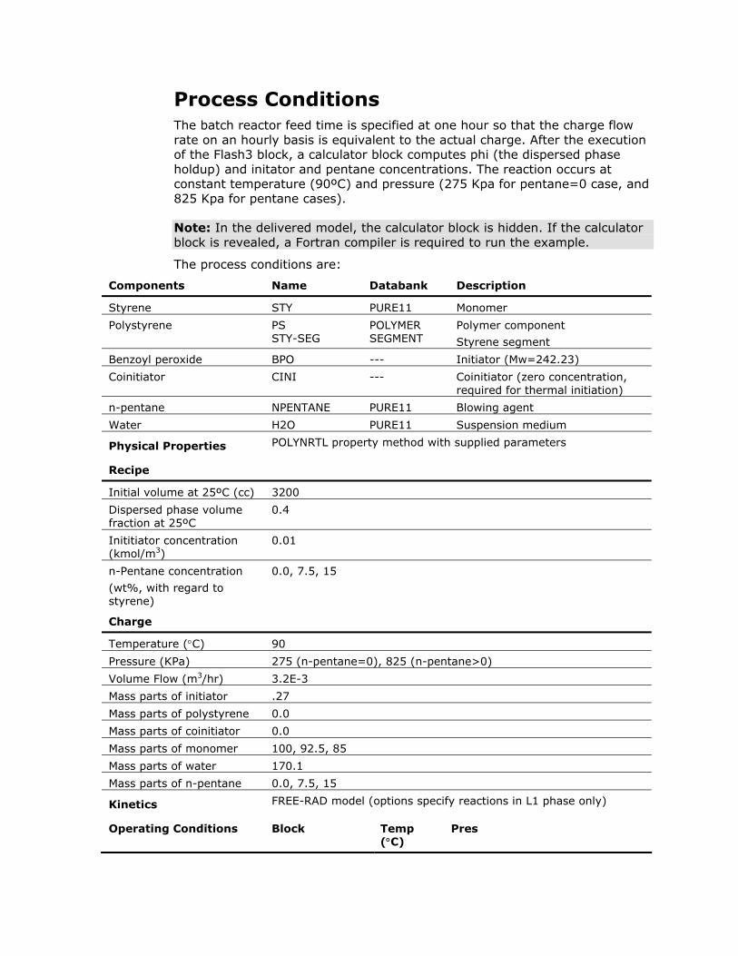
Process Conditions The batch reactor feed time is specified at one hour so that the charge flow rate on an hourly basis is equivalent to the actual charge. After the execution of the Flash3 block, a calculator block computes phi (the dispersed phase holdup) and initator and pentane concentrations. The reaction occurs at constant temperature (90ºC) and pressure (275 Kpa for pentane=0 case, and 825 Kpa for pentane cases).
Note: In the delivered model, the calculator block is hidden. If the calculator block is revealed, a Fortran compiler is required to run the example.
The process conditions are:
Components Name Databank Description
Styrene STY PURE11 Monomer
Polystyrene PS STY-SEG
POLYMER SEGMENT
Polymer component
Styrene segment
Benzoyl peroxide BPO --- Initiator (Mw=242.23)
Coinitiator CINI --- Coinitiator (zero concentration, required for thermal initiation)
n-pentane NPENTANE PURE11 Blowing agent
Water H2O PURE11 Suspension medium
Physical Properties POLYNRTL property method with supplied parameters
Recipe
Initial volume at 25ºC (cc) 3200
Dispersed phase volume fraction at 25ºC
0.4
Inititiator concentration (kmol/m3)
0.01
n-Pentane concentration
(wt%, with regard to styrene)
0.0, 7.5, 15
Charge
Temperature (°C) 90
Pressure (KPa) 275 (n-pentane=0), 825 (n-pentane>0)
Volume Flow (m3/hr) 3.2E-3
Mass parts of initiator .27
Mass parts of polystyrene 0.0
Mass parts of coinitiator 0.0
Mass parts of monomer 100, 92.5, 85
Mass parts of water 170.1
Mass parts of n-pentane 0.0, 7.5, 15
Kinetics FREE-RAD model (options specify reactions in L1 phase only)
Operating Conditions Block Temp (°C)
Pres
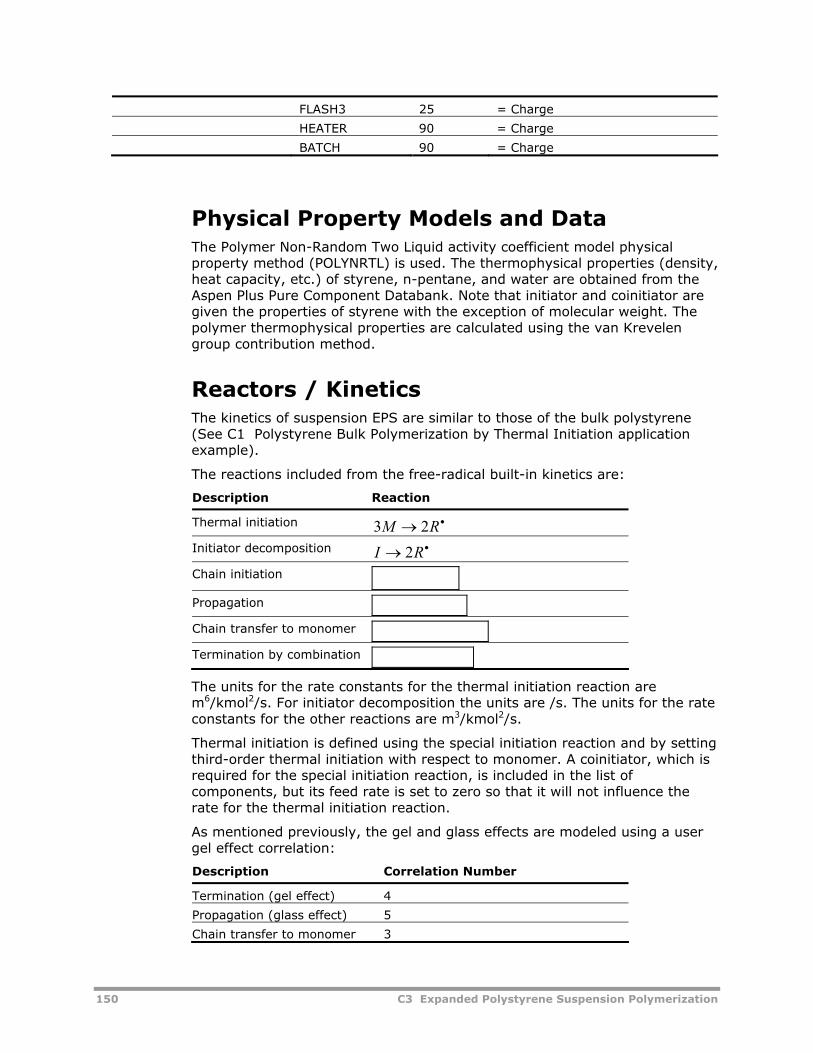
150 C3 Expanded Polystyrene Suspension Polymerization
FLASH3 25 = Charge
HEATER 90 = Charge
BATCH 90 = Charge
Physical Property Models and Data The Polymer Non-Random Two Liquid activity coefficient model physical property method (POLYNRTL) is used. The thermophysical properties (density, heat capacity, etc.) of styrene, n-pentane, and water are obtained from the Aspen Plus Pure Component Databank. Note that initiator and coinitiator are given the properties of styrene with the exception of molecular weight. The polymer thermophysical properties are calculated using the van Krevelen group contribution method.
Reactors / Kinetics The kinetics of suspension EPS are similar to those of the bulk polystyrene (See C1 Polystyrene Bulk Polymerization by Thermal Initiation application example).
The reactions included from the free-radical built-in kinetics are:
Description Reaction
Thermal initiation •→ RM 23
Initiator decomposition •→ RI 2
Chain initiation
Propagation
Chain transfer to monomer
Termination by combination
The units for the rate constants for the thermal initiation reaction are m6/kmol2/s. For initiator decomposition the units are /s. The units for the rate constants for the other reactions are m3/kmol2/s.
Thermal initiation is defined using the special initiation reaction and by setting third-order thermal initiation with respect to monomer. A coinitiator, which is required for the special initiation reaction, is included in the list of components, but its feed rate is set to zero so that it will not influence the rate for the thermal initiation reaction.
As mentioned previously, the gel and glass effects are modeled using a user gel effect correlation:
Description Correlation Number
Termination (gel effect) 4
Propagation (glass effect) 5
Chain transfer to monomer 3
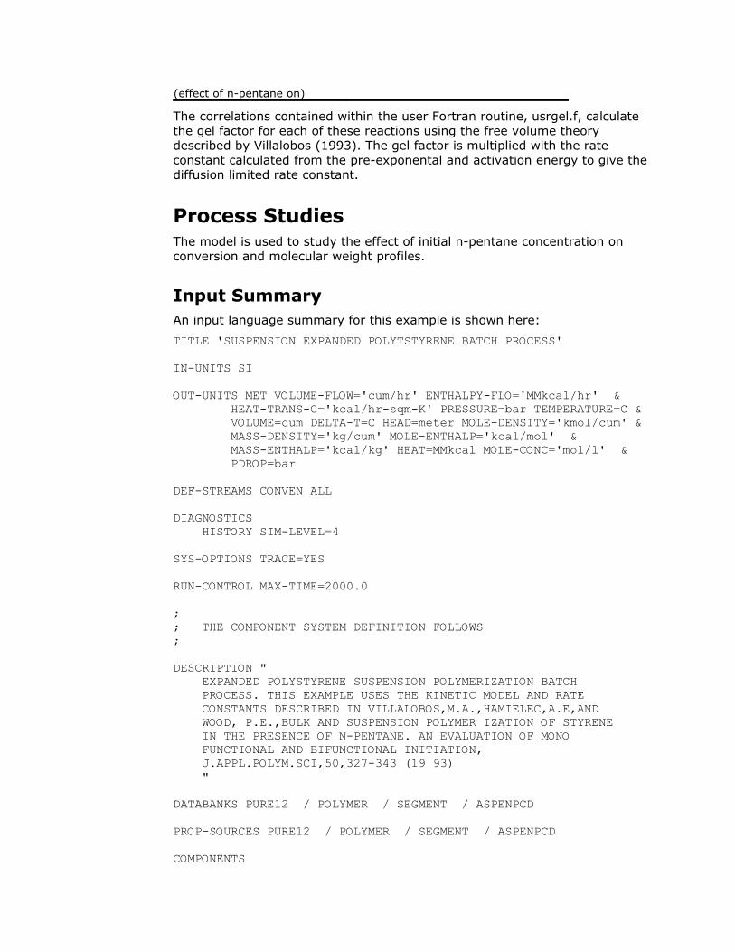
(effect of n-pentane on)
The correlations contained within the user Fortran routine, usrgel.f, calculate the gel factor for each of these reactions using the free volume theory described by Villalobos (1993). The gel factor is multiplied with the rate constant calculated from the pre-exponental and activation energy to give the diffusion limited rate constant.
Process Studies The model is used to study the effect of initial n-pentane concentration on conversion and molecular weight profiles.
Input Summary An input language summary for this example is shown here:
TITLE 'SUSPENSION EXPANDED POLYTSTYRENE BATCH PROCESS' IN-UNITS SI OUT-UNITS MET VOLUME-FLOW='cum/hr' ENTHALPY-FLO='MMkcal/hr' & HEAT-TRANS-C='kcal/hr-sqm-K' PRESSURE=bar TEMPERATURE=C & VOLUME=cum DELTA-T=C HEAD=meter MOLE-DENSITY='kmol/cum' & MASS-DENSITY='kg/cum' MOLE-ENTHALP='kcal/mol' & MASS-ENTHALP='kcal/kg' HEAT=MMkcal MOLE-CONC='mol/l' & PDROP=bar DEF-STREAMS CONVEN ALL DIAGNOSTICS HISTORY SIM-LEVEL=4 SYS-OPTIONS TRACE=YES RUN-CONTROL MAX-TIME=2000.0 ; ; THE COMPONENT SYSTEM DEFINITION FOLLOWS ; DESCRIPTION " EXPANDED POLYSTYRENE SUSPENSION POLYMERIZATION BATCH PROCESS. THIS EXAMPLE USES THE KINETIC MODEL AND RATE CONSTANTS DESCRIBED IN VILLALOBOS,M.A.,HAMIELEC,A.E,AND WOOD, P.E.,BULK AND SUSPENSION POLYMER IZATION OF STYRENE IN THE PRESENCE OF N-PENTANE. AN EVALUATION OF MONO FUNCTIONAL AND BIFUNCTIONAL INITIATION, J.APPL.POLYM.SCI,50,327-343 (19 93) " DATABANKS PURE12 / POLYMER / SEGMENT / ASPENPCD PROP-SOURCES PURE12 / POLYMER / SEGMENT / ASPENPCD COMPONENTS
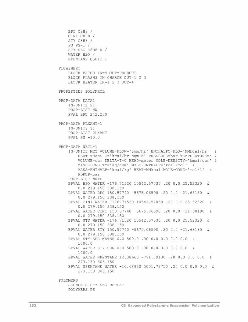
152 C3 Expanded Polystyrene Suspension Polymerization
BPO C8H8 / CINI C8H8 / STY C8H8 / PS PS-1 / STY-SEG C8H8-R / WATER H2O / NPENTANE C5H12-1 FLOWSHEET BLOCK BATCH IN=4 OUT=PRODUCT BLOCK FLASH3 IN=CHARGE OUT=1 2 3 BLOCK HEATER IN=1 2 3 OUT=4 PROPERTIES POLYNRTL PROP-DATA DATA1 IN-UNITS SI PROP-LIST MW PVAL BPO 242.230 PROP-DATA PLXANT-1 IN-UNITS SI PROP-LIST PLXANT PVAL PS -10.0 PROP-DATA NRTL-1 IN-UNITS MET VOLUME-FLOW='cum/hr' ENTHALPY-FLO='MMkcal/hr' & HEAT-TRANS-C='kcal/hr-sqm-K' PRESSURE=bar TEMPERATURE=K & VOLUME=cum DELTA-T=C HEAD=meter MOLE-DENSITY='kmol/cum' & MASS-DENSITY='kg/cum' MOLE-ENTHALP='kcal/mol' & MASS-ENTHALP='kcal/kg' HEAT=MMkcal MOLE-CONC='mol/l' & PDROP=bar PROP-LIST NRTL BPVAL BPO WATER -176.71520 10542.57030 .20 0.0 25.52320 & 0.0 279.150 338.150 BPVAL WATER BPO 150.57740 -5675.06590 .20 0.0 -21.68180 & 0.0 279.150 338.150 BPVAL CINI WATER -176.71520 10542.57030 .20 0.0 25.52320 & 0.0 279.150 338.150 BPVAL WATER CINI 150.57740 -5675.06590 .20 0.0 -21.68180 & 0.0 279.150 338.150 BPVAL STY WATER -176.71520 10542.57030 .20 0.0 25.52320 & 0.0 279.150 338.150 BPVAL WATER STY 150.57740 -5675.06590 .20 0.0 -21.68180 & 0.0 279.150 338.150 BPVAL STY-SEG WATER 0.0 500.0 .30 0.0 0.0 0.0 0.0 & 1000.0 BPVAL WATER STY-SEG 0.0 500.0 .30 0.0 0.0 0.0 0.0 & 1000.0 BPVAL WATER NPENTANE 12.38660 -791.79130 .20 0.0 0.0 0.0 & 273.150 303.150 BPVAL NPENTANE WATER -10.68920 5051.72750 .20 0.0 0.0 0.0 & 273.150 303.150 POLYMERS SEGMENTS STY-SEG REPEAT POLYMERS PS
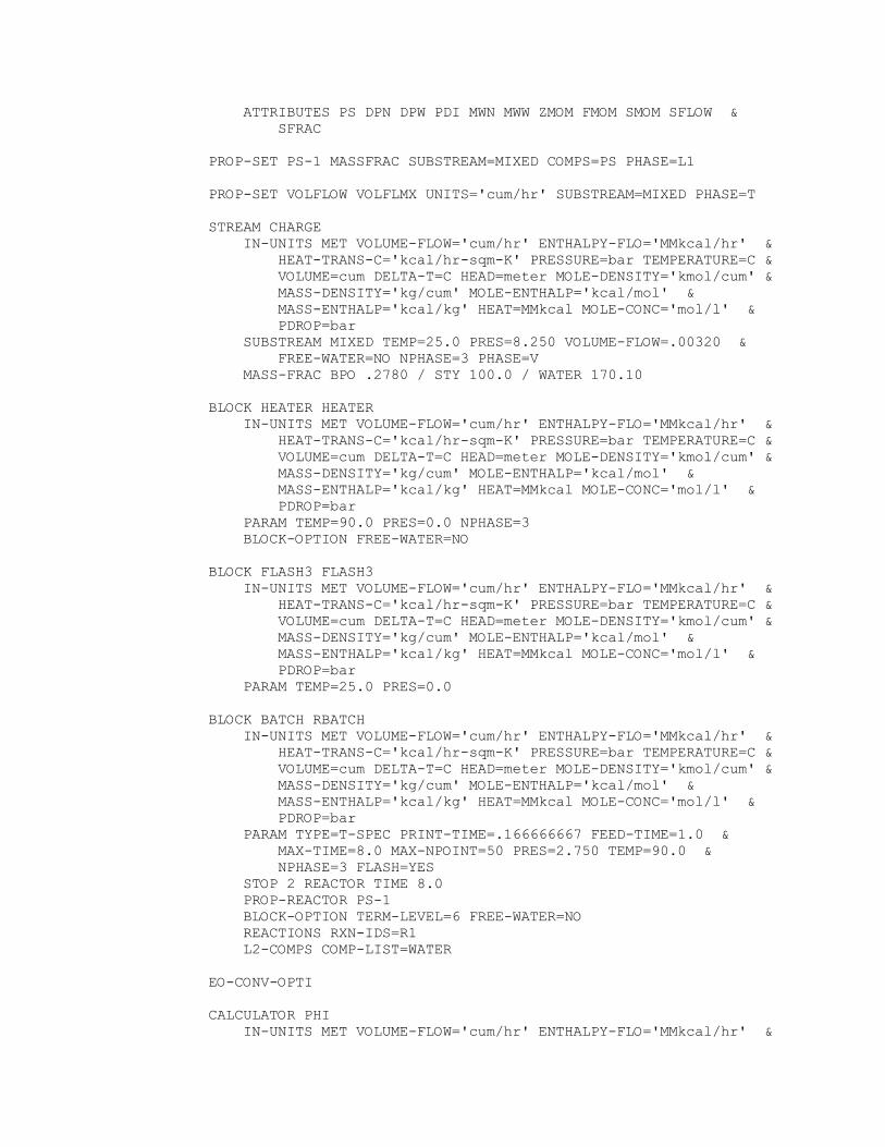
ATTRIBUTES PS DPN DPW PDI MWN MWW ZMOM FMOM SMOM SFLOW & SFRAC PROP-SET PS-1 MASSFRAC SUBSTREAM=MIXED COMPS=PS PHASE=L1 PROP-SET VOLFLOW VOLFLMX UNITS='cum/hr' SUBSTREAM=MIXED PHASE=T STREAM CHARGE IN-UNITS MET VOLUME-FLOW='cum/hr' ENTHALPY-FLO='MMkcal/hr' & HEAT-TRANS-C='kcal/hr-sqm-K' PRESSURE=bar TEMPERATURE=C & VOLUME=cum DELTA-T=C HEAD=meter MOLE-DENSITY='kmol/cum' & MASS-DENSITY='kg/cum' MOLE-ENTHALP='kcal/mol' & MASS-ENTHALP='kcal/kg' HEAT=MMkcal MOLE-CONC='mol/l' & PDROP=bar SUBSTREAM MIXED TEMP=25.0 PRES=8.250 VOLUME-FLOW=.00320 & FREE-WATER=NO NPHASE=3 PHASE=V MASS-FRAC BPO .2780 / STY 100.0 / WATER 170.10 BLOCK HEATER HEATER IN-UNITS MET VOLUME-FLOW='cum/hr' ENTHALPY-FLO='MMkcal/hr' & HEAT-TRANS-C='kcal/hr-sqm-K' PRESSURE=bar TEMPERATURE=C & VOLUME=cum DELTA-T=C HEAD=meter MOLE-DENSITY='kmol/cum' & MASS-DENSITY='kg/cum' MOLE-ENTHALP='kcal/mol' & MASS-ENTHALP='kcal/kg' HEAT=MMkcal MOLE-CONC='mol/l' & PDROP=bar PARAM TEMP=90.0 PRES=0.0 NPHASE=3 BLOCK-OPTION FREE-WATER=NO BLOCK FLASH3 FLASH3 IN-UNITS MET VOLUME-FLOW='cum/hr' ENTHALPY-FLO='MMkcal/hr' & HEAT-TRANS-C='kcal/hr-sqm-K' PRESSURE=bar TEMPERATURE=C & VOLUME=cum DELTA-T=C HEAD=meter MOLE-DENSITY='kmol/cum' & MASS-DENSITY='kg/cum' MOLE-ENTHALP='kcal/mol' & MASS-ENTHALP='kcal/kg' HEAT=MMkcal MOLE-CONC='mol/l' & PDROP=bar PARAM TEMP=25.0 PRES=0.0 BLOCK BATCH RBATCH IN-UNITS MET VOLUME-FLOW='cum/hr' ENTHALPY-FLO='MMkcal/hr' & HEAT-TRANS-C='kcal/hr-sqm-K' PRESSURE=bar TEMPERATURE=C & VOLUME=cum DELTA-T=C HEAD=meter MOLE-DENSITY='kmol/cum' & MASS-DENSITY='kg/cum' MOLE-ENTHALP='kcal/mol' & MASS-ENTHALP='kcal/kg' HEAT=MMkcal MOLE-CONC='mol/l' & PDROP=bar PARAM TYPE=T-SPEC PRINT-TIME=.166666667 FEED-TIME=1.0 & MAX-TIME=8.0 MAX-NPOINT=50 PRES=2.750 TEMP=90.0 & NPHASE=3 FLASH=YES STOP 2 REACTOR TIME 8.0 PROP-REACTOR PS-1 BLOCK-OPTION TERM-LEVEL=6 FREE-WATER=NO REACTIONS RXN-IDS=R1 L2-COMPS COMP-LIST=WATER EO-CONV-OPTI CALCULATOR PHI IN-UNITS MET VOLUME-FLOW='cum/hr' ENTHALPY-FLO='MMkcal/hr' &
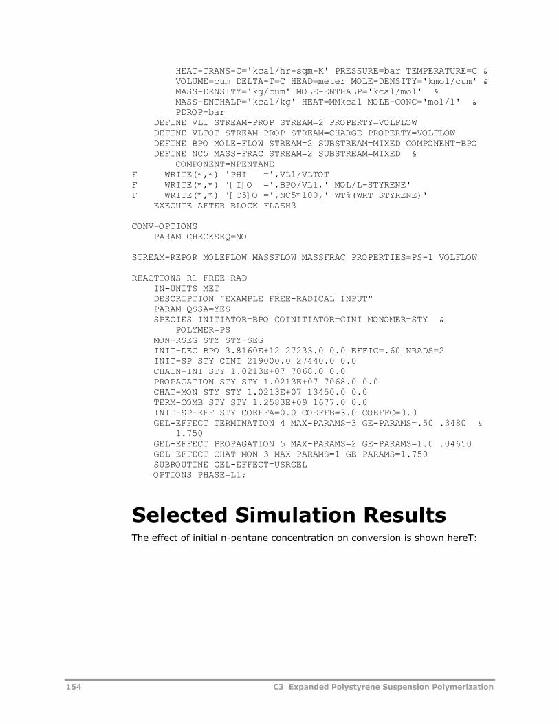
154 C3 Expanded Polystyrene Suspension Polymerization
HEAT-TRANS-C='kcal/hr-sqm-K' PRESSURE=bar TEMPERATURE=C & VOLUME=cum DELTA-T=C HEAD=meter MOLE-DENSITY='kmol/cum' & MASS-DENSITY='kg/cum' MOLE-ENTHALP='kcal/mol' & MASS-ENTHALP='kcal/kg' HEAT=MMkcal MOLE-CONC='mol/l' & PDROP=bar DEFINE VL1 STREAM-PROP STREAM=2 PROPERTY=VOLFLOW DEFINE VLTOT STREAM-PROP STREAM=CHARGE PROPERTY=VOLFLOW DEFINE BPO MOLE-FLOW STREAM=2 SUBSTREAM=MIXED COMPONENT=BPO DEFINE NC5 MASS-FRAC STREAM=2 SUBSTREAM=MIXED & COMPONENT=NPENTANE F WRITE(*,*) 'PHI =',VL1/VLTOT F WRITE(*,*) '[I]O =',BPO/VL1,' MOL/L-STYRENE' F WRITE(*,*) '[C5]O =',NC5*100,' WT%(WRT STYRENE)' EXECUTE AFTER BLOCK FLASH3 CONV-OPTIONS PARAM CHECKSEQ=NO STREAM-REPOR MOLEFLOW MASSFLOW MASSFRAC PROPERTIES=PS-1 VOLFLOW REACTIONS R1 FREE-RAD IN-UNITS MET DESCRIPTION "EXAMPLE FREE-RADICAL INPUT" PARAM QSSA=YES SPECIES INITIATOR=BPO COINITIATOR=CINI MONOMER=STY & POLYMER=PS MON-RSEG STY STY-SEG INIT-DEC BPO 3.8160E+12 27233.0 0.0 EFFIC=.60 NRADS=2 INIT-SP STY CINI 219000.0 27440.0 0.0 CHAIN-INI STY 1.0213E+07 7068.0 0.0 PROPAGATION STY STY 1.0213E+07 7068.0 0.0 CHAT-MON STY STY 1.0213E+07 13450.0 0.0 TERM-COMB STY STY 1.2583E+09 1677.0 0.0 INIT-SP-EFF STY COEFFA=0.0 COEFFB=3.0 COEFFC=0.0 GEL-EFFECT TERMINATION 4 MAX-PARAMS=3 GE-PARAMS=.50 .3480 & 1.750 GEL-EFFECT PROPAGATION 5 MAX-PARAMS=2 GE-PARAMS=1.0 .04650 GEL-EFFECT CHAT-MON 3 MAX-PARAMS=1 GE-PARAMS=1.750 SUBROUTINE GEL-EFFECT=USRGEL OPTIONS PHASE=L1;
Selected Simulation Results The effect of initial n-pentane concentration on conversion is shown hereT:
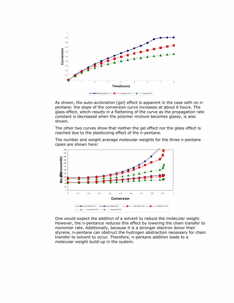
0
0.1
0.2
0.3
0.4
0.5
0.6
0.7
0.8
0.9
1
0 1 2 3 4 5 6 7 8
Time(hours)
Con
vers
ion
n-pentane=0 n-pentane=7.5% n-pentane=15%
As shown, the auto-accleration (gel) effect is apparent in the case with no n-pentane: the slope of the conversion curve increases at about 6 hours. The glass effect, which results in a flattening of the curve as the propagation rate constant is decreased when the polymer mixture becomes glassy, is also shown.
The other two curves show that neither the gel effect nor the glass effect is reached due to the plasticizing effect of the n-pentane.
The number and weight average molecular weights for the three n-pentane cases are shown here:
0
25
50
75
100
125
150
175
200
225
250
275
300
0 0.1 0.2 0.3 0.4 0.5 0.6 0.7 0.8 0.9 1
(Tho
usan
ds)
Conversion
Mn,
Mw
npentane=0 npentane=0 npentane=7.5% npentane=7.5%
n-pentane=15% n-pentane=15%
One would expect the addition of a solvent to reduce the molecular weight. However, the n-pentance reduces this effect by lowering the chain transfer to monomer rate. Additionally, because it is a stronger electron donor than styrene, n-pentane can obstruct the hydrogen abstraction necessary for chain transfer to solvent to occur. Therefore, n-pentane addition leads to a molecular weight build-up in the system.
156 C3 Expanded Polystyrene Suspension Polymerization
References Villalobos, M. A., Hamielec,A. E., & Wood, P. E. (1993). Bulk and Suspension Polymerization of Styrene in the Presence of n-Pentane. An Evaluation of Monofunctional and Bifunctional Initiation. J. Appl. Polym. Sci., 50, 327-343.
C4 Styrene Ethyl Acrylate Free-Radical Copolymerization Process
The styrene ethyl acrylate free-radical copolymerization model illustrates the use of Aspen Polymers Plus to model a styrene ethyl acrylate free-radical process. The process modeled is an experimental system developed by McManus and Penlidis at the University of Waterloo. The model is then used along with the experimental data generated at the University of Waterloo to estimate reaction rate constant parameters.
About This Process The copolymerization of styrene with ethyl acrylate is of considerable interest to the polymer industry. In 1996, McManus and Penlidis from the University of Waterloo reported a detailed study of the copolymerization of styrene and ethyl acrylate, and generated extensive data by varying the initiator concentration, feed composition, and the reactor temperature (McManus & Penlidis, 1996). Similar studies have been done for this system (Fehervari et al., 1981). A number of investigators estimated the kinetic parameters, but there are many discrepancies between kinetic rate constants and the reactivity ratios reported in the literature. McManus and Penlidis reviewed the information available on the kinetic data and estimated the reactivity ratios.
Process Definition The copolymerization of styrene and ethyl acrylate is carried out in a batch reactor. The batch reactor is charged with a pre-mixed stream of styrene, ethyl acrylate, and the initiator azo-bis-isobutyronitrile. The reactor is operated at a constant temperature and pressure. The flowsheet is shown here:
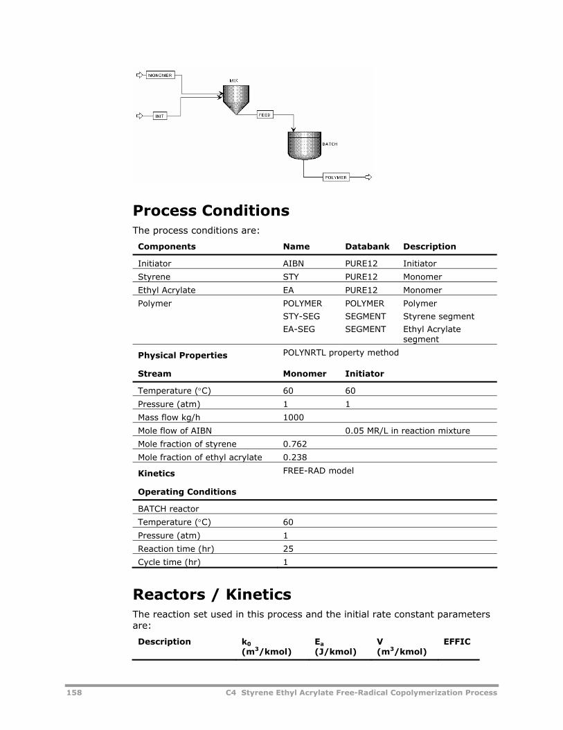
158 C4 Styrene Ethyl Acrylate Free-Radical Copolymerization Process
Process Conditions The process conditions are:
Components Name Databank Description
Initiator AIBN PURE12 Initiator
Styrene STY PURE12 Monomer
Ethyl Acrylate EA PURE12 Monomer
Polymer POLYMER
STY-SEG
EA-SEG
POLYMER
SEGMENT
SEGMENT
Polymer
Styrene segment
Ethyl Acrylate segment
Physical Properties POLYNRTL property method
Stream Monomer Initiator
Temperature (°C) 60 60
Pressure (atm) 1 1
Mass flow kg/h 1000
Mole flow of AIBN 0.05 MR/L in reaction mixture
Mole fraction of styrene 0.762
Mole fraction of ethyl acrylate 0.238
Kinetics FREE-RAD model
Operating Conditions
BATCH reactor
Temperature (°C) 60
Pressure (atm) 1
Reaction time (hr) 25
Cycle time (hr) 1
Reactors / Kinetics The reaction set used in this process and the initial rate constant parameters are:
Description k0 (m3/kmol)
Ea (J/kmol)
V (m3/kmol)
EFFIC
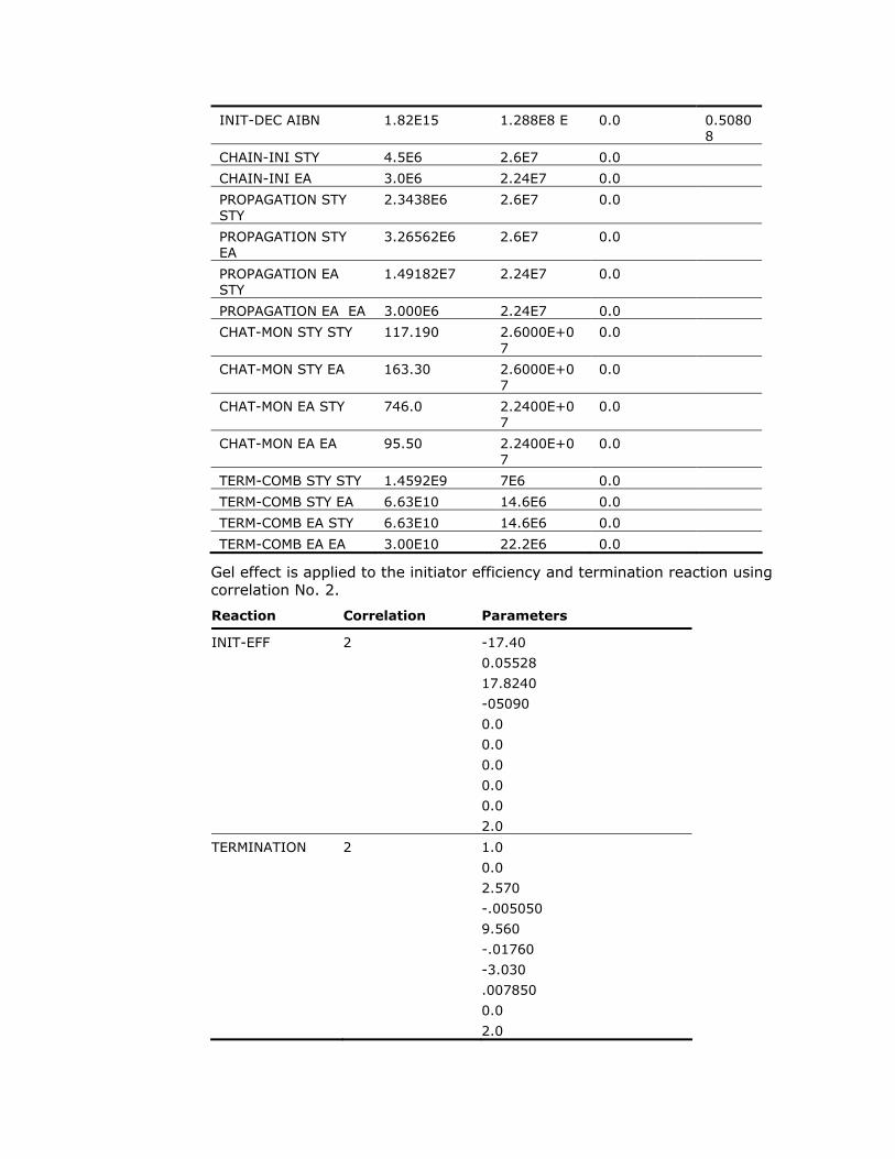
INIT-DEC AIBN 1.82E15 1.288E8 E 0.0 0.50808
CHAIN-INI STY 4.5E6 2.6E7 0.0
CHAIN-INI EA 3.0E6 2.24E7 0.0
PROPAGATION STY STY
2.3438E6 2.6E7 0.0
PROPAGATION STY EA
3.26562E6 2.6E7 0.0
PROPAGATION EA STY
1.49182E7 2.24E7 0.0
PROPAGATION EA EA 3.000E6 2.24E7 0.0
CHAT-MON STY STY 117.190 2.6000E+07
0.0
CHAT-MON STY EA 163.30 2.6000E+07
0.0
CHAT-MON EA STY 746.0 2.2400E+07
0.0
CHAT-MON EA EA 95.50 2.2400E+07
0.0
TERM-COMB STY STY 1.4592E9 7E6 0.0
TERM-COMB STY EA 6.63E10 14.6E6 0.0
TERM-COMB EA STY 6.63E10 14.6E6 0.0
TERM-COMB EA EA 3.00E10 22.2E6 0.0
Gel effect is applied to the initiator efficiency and termination reaction using correlation No. 2.
Reaction Correlation Parameters
INIT-EFF 2 -17.40
0.05528
17.8240
-05090
0.0
0.0
0.0
0.0
0.0
2.0
TERMINATION 2 1.0
0.0
2.570
-.005050
9.560
-.01760
-3.030
.007850
0.0
2.0
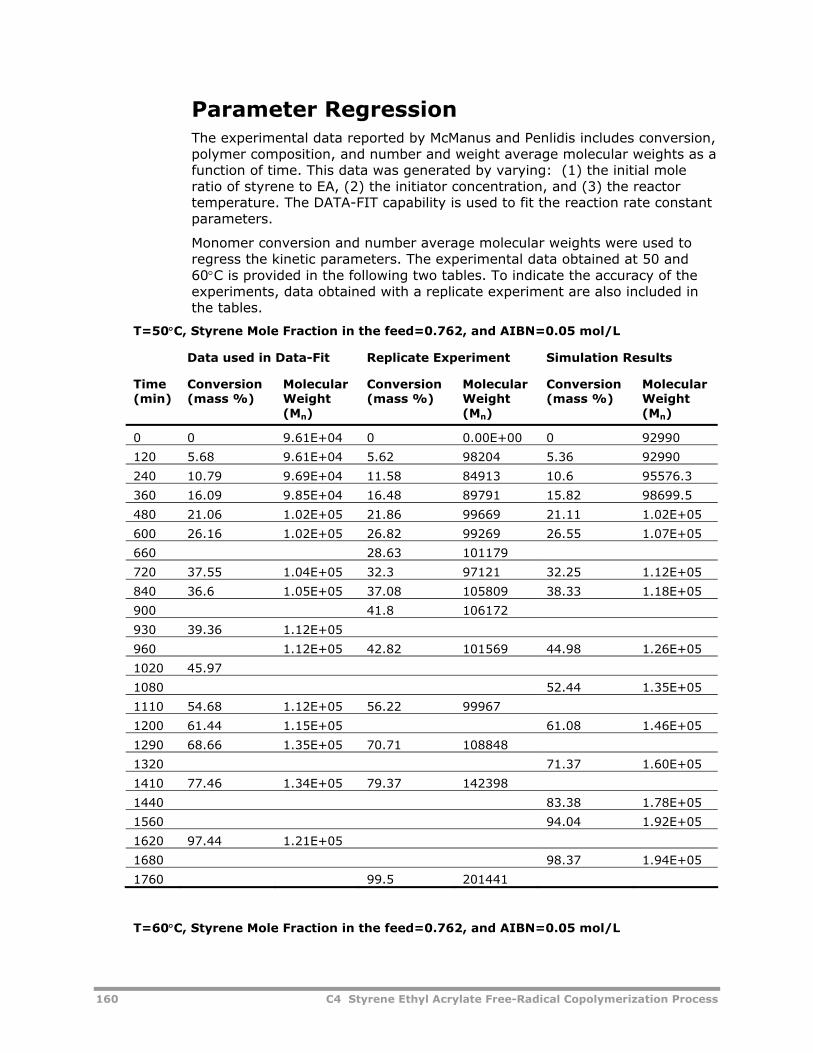
160 C4 Styrene Ethyl Acrylate Free-Radical Copolymerization Process
Parameter Regression The experimental data reported by McManus and Penlidis includes conversion, polymer composition, and number and weight average molecular weights as a function of time. This data was generated by varying: (1) the initial mole ratio of styrene to EA, (2) the initiator concentration, and (3) the reactor temperature. The DATA-FIT capability is used to fit the reaction rate constant parameters.
Monomer conversion and number average molecular weights were used to regress the kinetic parameters. The experimental data obtained at 50 and 60°C is provided in the following two tables. To indicate the accuracy of the experiments, data obtained with a replicate experiment are also included in the tables.
T=50°C, Styrene Mole Fraction in the feed=0.762, and AIBN=0.05 mol/L
Data used in Data-Fit Replicate Experiment Simulation Results
Time (min)
Conversion (mass %)
Molecular Weight (Mn)
Conversion (mass %)
Molecular Weight (Mn)
Conversion (mass %)
Molecular Weight (Mn)
0 0 9.61E+04 0 0.00E+00 0 92990
120 5.68 9.61E+04 5.62 98204 5.36 92990
240 10.79 9.69E+04 11.58 84913 10.6 95576.3
360 16.09 9.85E+04 16.48 89791 15.82 98699.5
480 21.06 1.02E+05 21.86 99669 21.11 1.02E+05
600 26.16 1.02E+05 26.82 99269 26.55 1.07E+05
660 28.63 101179
720 37.55 1.04E+05 32.3 97121 32.25 1.12E+05
840 36.6 1.05E+05 37.08 105809 38.33 1.18E+05
900 41.8 106172
930 39.36 1.12E+05
960 1.12E+05 42.82 101569 44.98 1.26E+05
1020 45.97
1080 52.44 1.35E+05
1110 54.68 1.12E+05 56.22 99967
1200 61.44 1.15E+05 61.08 1.46E+05
1290 68.66 1.35E+05 70.71 108848
1320 71.37 1.60E+05
1410 77.46 1.34E+05 79.37 142398
1440 83.38 1.78E+05
1560 94.04 1.92E+05
1620 97.44 1.21E+05
1680 98.37 1.94E+05
1760 99.5 201441
T=60°C, Styrene Mole Fraction in the feed=0.762, and AIBN=0.05 mol/L
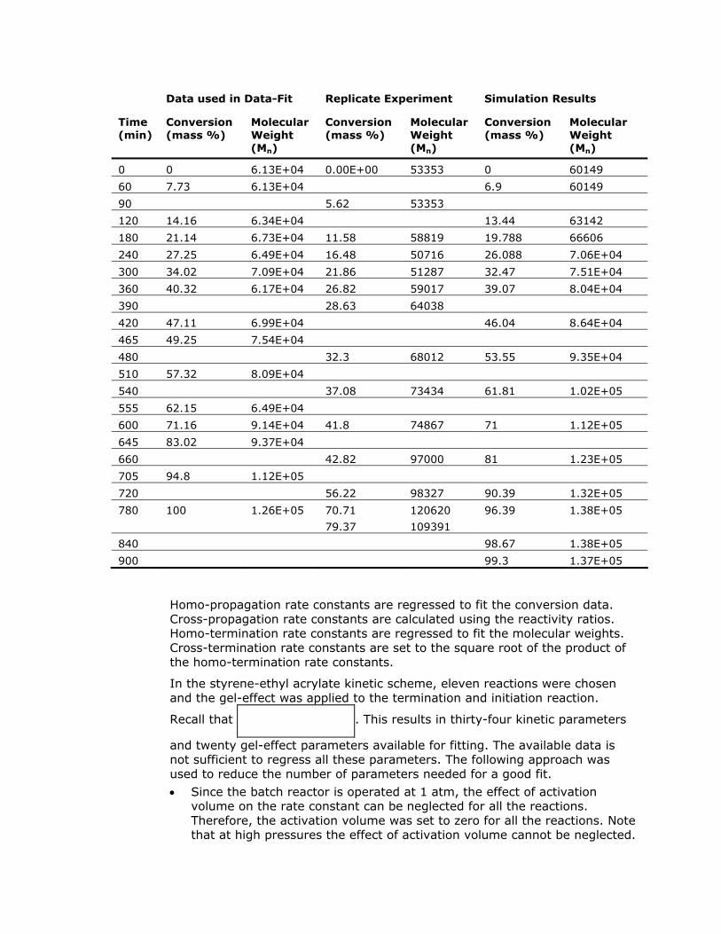
Data used in Data-Fit Replicate Experiment Simulation Results
Time (min)
Conversion (mass %)
Molecular Weight (Mn)
Conversion (mass %)
Molecular Weight (Mn)
Conversion (mass %)
Molecular Weight (Mn)
0 0 6.13E+04 0.00E+00 53353 0 60149
60 7.73 6.13E+04 6.9 60149
90 5.62 53353
120 14.16 6.34E+04 13.44 63142
180 21.14 6.73E+04 11.58 58819 19.788 66606
240 27.25 6.49E+04 16.48 50716 26.088 7.06E+04
300 34.02 7.09E+04 21.86 51287 32.47 7.51E+04
360 40.32 6.17E+04 26.82 59017 39.07 8.04E+04
390 28.63 64038
420 47.11 6.99E+04 46.04 8.64E+04
465 49.25 7.54E+04
480 32.3 68012 53.55 9.35E+04
510 57.32 8.09E+04
540 37.08 73434 61.81 1.02E+05
555 62.15 6.49E+04
600 71.16 9.14E+04 41.8 74867 71 1.12E+05
645 83.02 9.37E+04
660 42.82 97000 81 1.23E+05
705 94.8 1.12E+05
720 56.22 98327 90.39 1.32E+05
780 100 1.26E+05 70.71
79.37
120620
109391
96.39 1.38E+05
840 98.67 1.38E+05
900 99.3 1.37E+05
Homo-propagation rate constants are regressed to fit the conversion data. Cross-propagation rate constants are calculated using the reactivity ratios. Homo-termination rate constants are regressed to fit the molecular weights. Cross-termination rate constants are set to the square root of the product of the homo-termination rate constants.
In the styrene-ethyl acrylate kinetic scheme, eleven reactions were chosen and the gel-effect was applied to the termination and initiation reaction.
Recall that . This results in thirty-four kinetic parameters
and twenty gel-effect parameters available for fitting. The available data is not sufficient to regress all these parameters. The following approach was used to reduce the number of parameters needed for a good fit.
• Since the batch reactor is operated at 1 atm, the effect of activation volume on the rate constant can be neglected for all the reactions. Therefore, the activation volume was set to zero for all the reactions. Note that at high pressures the effect of activation volume cannot be neglected.
162 C4 Styrene Ethyl Acrylate Free-Radical Copolymerization Process
• The initiator decomposition rate constants were known. Typically these can be obtained from a good polymer handbook or from the supplier. They can also be calculated using the half-life data. (See Appendix B of the Aspen Polymers Plus User Guide, Volume 1).
• Chain initiation rate constants are in general faster than the propagation rate constants. Therefore these constants were set to be the same or greater than the propagation rate constants.
• There are two homo-propagation reactions and two cross-propagation reactions in the kinetic scheme. The number of regressable parameters is then eight excluding the activation volume parameters.
• The number of regressable propagation parameters can be reduced if the homo-propagation rate constants and/or the reactivity ratios are known. If the homo-propagation rate constants are known then reactivity ratios can be estimated. If the reactivity ratios are known homo-propagation rate constants can be estimated. In this example, reactivity ratios were given (Fehervari et al., 1981), and the homo-propagation rate constants were regressed. The cross-propagation rate constants were calculated using the following equations:
Where:
STY=1
EA=2
• Four termination reactions are considered in this scheme. Cross-termination reactions involving STY and EA segments were set to have the same rate constant. This reduces specification of the rate constants to three. If the homo-termination rate constants are known, the cross-termination rate constants can be estimated using the following equations:
In this example homo-termination rate constants were regressed using the molecular weight data.
• In the kinetic scheme termination by combination was selected. It is possible that termination by disproportionation can also occur. One needs to know apriori the termination mechanism. As a general rule if polydispersity (PDI) is 1.5 termination by combination is controlling and if PDI is two termination is controlled by the disproportionation reaction.
• At high conversion termination is diffusion controlled. This is modeled using the gel-effect option. Therefore use of low conversion data is recommended for regression of the kinetic parameters without using gel-effect. High conversion data is then used to regress the gel-effect parameters.
• Monomer conversion data was used to regress the initiator efficiency, propagation and the termination rate constants. Molecular weight data was used to regress the propagation and the termination rate constants.
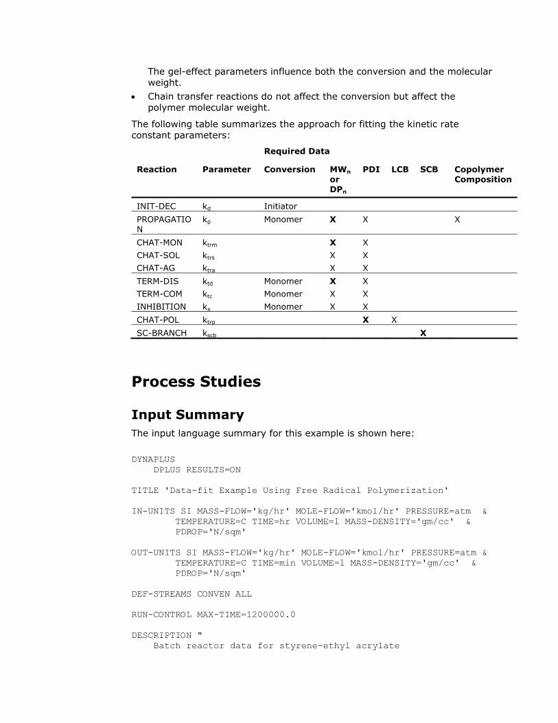
The gel-effect parameters influence both the conversion and the molecular weight.
• Chain transfer reactions do not affect the conversion but affect the polymer molecular weight.
The following table summarizes the approach for fitting the kinetic rate constant parameters:
Required Data
Reaction Parameter Conversion MWn or DPn
PDI LCB SCB Copolymer Composition
INIT-DEC kd Initiator
PROPAGATION
kp Monomer X X X
CHAT-MON
CHAT-SOL
CHAT-AG
ktrm
ktrs
ktra
X
X
X
X
X
X
TERM-DIS
TERM-COM
INHIBITION
ktd
ktc
kx
Monomer
Monomer
Monomer
X
X
X
X
X
X
CHAT-POL ktrp X X
SC-BRANCH kscb X
Process Studies
Input Summary The input language summary for this example is shown here:
DYNAPLUS DPLUS RESULTS=ON TITLE 'Data-fit Example Using Free Radical Polymerization' IN-UNITS SI MASS-FLOW='kg/hr' MOLE-FLOW='kmol/hr' PRESSURE=atm & TEMPERATURE=C TIME=hr VOLUME=l MASS-DENSITY='gm/cc' & PDROP='N/sqm' OUT-UNITS SI MASS-FLOW='kg/hr' MOLE-FLOW='kmol/hr' PRESSURE=atm & TEMPERATURE=C TIME=min VOLUME=l MASS-DENSITY='gm/cc' & PDROP='N/sqm' DEF-STREAMS CONVEN ALL RUN-CONTROL MAX-TIME=1200000.0 DESCRIPTION " Batch reactor data for styrene-ethyl acrylate
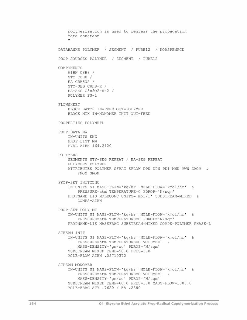
164 C4 Styrene Ethyl Acrylate Free-Radical Copolymerization Process
polymerization is used to regress the propagation rate constant " DATABANKS POLYMER / SEGMENT / PURE12 / NOASPENPCD PROP-SOURCES POLYMER / SEGMENT / PURE12 COMPONENTS AIBN C8H8 / STY C8H8 / EA C5H8O2 / STY-SEG C8H8-R / EA-SEG C5H8O2-R-2 / POLYMER PS-1 FLOWSHEET BLOCK BATCH IN=FEED OUT=POLYMER BLOCK MIX IN=MONOMER INIT OUT=FEED PROPERTIES POLYNRTL PROP-DATA MW IN-UNITS ENG PROP-LIST MW PVAL AIBN 164.2120 POLYMERS SEGMENTS STY-SEG REPEAT / EA-SEG REPEAT POLYMERS POLYMER ATTRIBUTES POLYMER SFRAC SFLOW DPN DPW PDI MWN MWW ZMOM & FMOM SMOM PROP-SET INITCONC IN-UNITS SI MASS-FLOW='kg/hr' MOLE-FLOW='kmol/hr' & PRESSURE=atm TEMPERATURE=C PDROP='N/sqm' PROPNAME-LIS MOLECONC UNITS='mol/l' SUBSTREAM=MIXED & COMPS=AIBN PROP-SET POLY-MF IN-UNITS SI MASS-FLOW='kg/hr' MOLE-FLOW='kmol/hr' & PRESSURE=atm TEMPERATURE=C PDROP='N/sqm' PROPNAME-LIS MASSFRAC SUBSTREAM=MIXED COMPS=POLYMER PHASE=L STREAM INIT IN-UNITS SI MASS-FLOW='kg/hr' MOLE-FLOW='kmol/hr' & PRESSURE=atm TEMPERATURE=C VOLUME=l & MASS-DENSITY='gm/cc' PDROP='N/sqm' SUBSTREAM MIXED TEMP=50.0 PRES=1.0 MOLE-FLOW AIBN .05710370 STREAM MONOMER IN-UNITS SI MASS-FLOW='kg/hr' MOLE-FLOW='kmol/hr' & PRESSURE=atm TEMPERATURE=C VOLUME=l & MASS-DENSITY='gm/cc' PDROP='N/sqm' SUBSTREAM MIXED TEMP=60.0 PRES=1.0 MASS-FLOW=1000.0 MOLE-FRAC STY .7620 / EA .2380
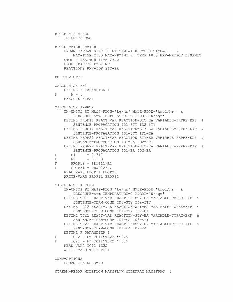
BLOCK MIX MIXER IN-UNITS ENG BLOCK BATCH RBATCH PARAM TYPE=T-SPEC PRINT-TIME=1.0 CYCLE-TIME=1.0 & MAX-TIME=25.0 MAX-NPOINT=27 TEMP=60.0 ERR-METHOD=DYNAMIC STOP 1 REACTOR TIME 25.0 PROP-REACTOR POLY-MF REACTIONS RXN-IDS=STY-EA EO-CONV-OPTI CALCULATOR F-1 DEFINE F PARAMETER 1 F F = 5 EXECUTE FIRST CALCULATOR K-PROP IN-UNITS SI MASS-FLOW='kg/hr' MOLE-FLOW='kmol/hr' & PRESSURE=atm TEMPERATURE=C PDROP='N/sqm' DEFINE PROP11 REACT-VAR REACTION=STY-EA VARIABLE=PRPRE-EXP & SENTENCE=PROPAGATION ID1=STY ID2=STY DEFINE PROP12 REACT-VAR REACTION=STY-EA VARIABLE=PRPRE-EXP & SENTENCE=PROPAGATION ID1=STY ID2=EA DEFINE PROP21 REACT-VAR REACTION=STY-EA VARIABLE=PRPRE-EXP & SENTENCE=PROPAGATION ID1=EA ID2=STY DEFINE PROP22 REACT-VAR REACTION=STY-EA VARIABLE=PRPRE-EXP & SENTENCE=PROPAGATION ID1=EA ID2=EA F R1 = 0.717 F R2 = 0.128 F PROP12 = PROP11/R1 F PROP21 = PROP22/R2 READ-VARS PROP11 PROP22 WRITE-VARS PROP12 PROP21 CALCULATOR K-TERM IN-UNITS SI MASS-FLOW='kg/hr' MOLE-FLOW='kmol/hr' & PRESSURE=atm TEMPERATURE=C PDROP='N/sqm' DEFINE TC11 REACT-VAR REACTION=STY-EA VARIABLE=TCPRE-EXP & SENTENCE=TERM-COMB ID1=STY ID2=STY DEFINE TC12 REACT-VAR REACTION=STY-EA VARIABLE=TCPRE-EXP & SENTENCE=TERM-COMB ID1=STY ID2=EA DEFINE TC21 REACT-VAR REACTION=STY-EA VARIABLE=TCPRE-EXP & SENTENCE=TERM-COMB ID1=EA ID2=STY DEFINE TC22 REACT-VAR REACTION=STY-EA VARIABLE=TCPRE-EXP & SENTENCE=TERM-COMB ID1=EA ID2=EA DEFINE F PARAMETER 1 F TC12 = F*(TC11*TC22)**0.5 F TC21 = F*(TC11*TC22)**0.5 READ-VARS TC11 TC22 WRITE-VARS TC12 TC21 CONV-OPTIONS PARAM CHECKSEQ=NO STREAM-REPOR MOLEFLOW MASSFLOW MOLEFRAC MASSFRAC &
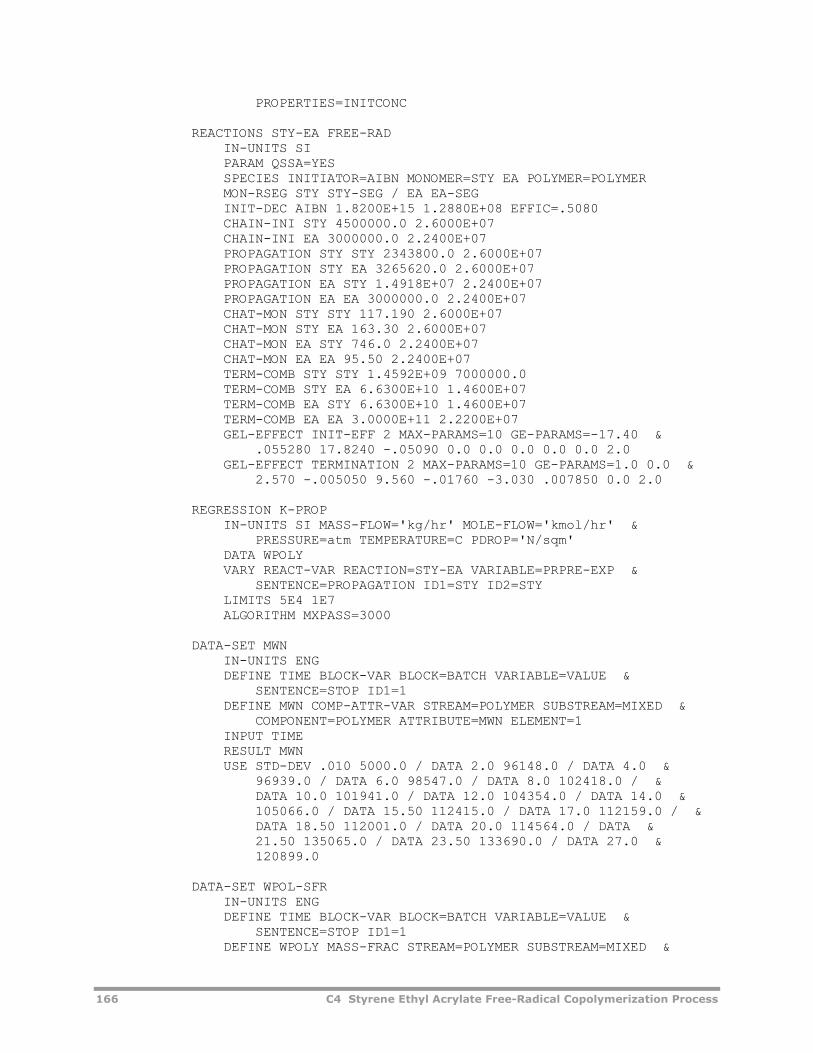
166 C4 Styrene Ethyl Acrylate Free-Radical Copolymerization Process
PROPERTIES=INITCONC REACTIONS STY-EA FREE-RAD IN-UNITS SI PARAM QSSA=YES SPECIES INITIATOR=AIBN MONOMER=STY EA POLYMER=POLYMER MON-RSEG STY STY-SEG / EA EA-SEG INIT-DEC AIBN 1.8200E+15 1.2880E+08 EFFIC=.5080 CHAIN-INI STY 4500000.0 2.6000E+07 CHAIN-INI EA 3000000.0 2.2400E+07 PROPAGATION STY STY 2343800.0 2.6000E+07 PROPAGATION STY EA 3265620.0 2.6000E+07 PROPAGATION EA STY 1.4918E+07 2.2400E+07 PROPAGATION EA EA 3000000.0 2.2400E+07 CHAT-MON STY STY 117.190 2.6000E+07 CHAT-MON STY EA 163.30 2.6000E+07 CHAT-MON EA STY 746.0 2.2400E+07 CHAT-MON EA EA 95.50 2.2400E+07 TERM-COMB STY STY 1.4592E+09 7000000.0 TERM-COMB STY EA 6.6300E+10 1.4600E+07 TERM-COMB EA STY 6.6300E+10 1.4600E+07 TERM-COMB EA EA 3.0000E+11 2.2200E+07 GEL-EFFECT INIT-EFF 2 MAX-PARAMS=10 GE-PARAMS=-17.40 & .055280 17.8240 -.05090 0.0 0.0 0.0 0.0 0.0 2.0 GEL-EFFECT TERMINATION 2 MAX-PARAMS=10 GE-PARAMS=1.0 0.0 & 2.570 -.005050 9.560 -.01760 -3.030 .007850 0.0 2.0 REGRESSION K-PROP IN-UNITS SI MASS-FLOW='kg/hr' MOLE-FLOW='kmol/hr' & PRESSURE=atm TEMPERATURE=C PDROP='N/sqm' DATA WPOLY VARY REACT-VAR REACTION=STY-EA VARIABLE=PRPRE-EXP & SENTENCE=PROPAGATION ID1=STY ID2=STY LIMITS 5E4 1E7 ALGORITHM MXPASS=3000 DATA-SET MWN IN-UNITS ENG DEFINE TIME BLOCK-VAR BLOCK=BATCH VARIABLE=VALUE & SENTENCE=STOP ID1=1 DEFINE MWN COMP-ATTR-VAR STREAM=POLYMER SUBSTREAM=MIXED & COMPONENT=POLYMER ATTRIBUTE=MWN ELEMENT=1 INPUT TIME RESULT MWN USE STD-DEV .010 5000.0 / DATA 2.0 96148.0 / DATA 4.0 & 96939.0 / DATA 6.0 98547.0 / DATA 8.0 102418.0 / & DATA 10.0 101941.0 / DATA 12.0 104354.0 / DATA 14.0 & 105066.0 / DATA 15.50 112415.0 / DATA 17.0 112159.0 / & DATA 18.50 112001.0 / DATA 20.0 114564.0 / DATA & 21.50 135065.0 / DATA 23.50 133690.0 / DATA 27.0 & 120899.0 DATA-SET WPOL-SFR IN-UNITS ENG DEFINE TIME BLOCK-VAR BLOCK=BATCH VARIABLE=VALUE & SENTENCE=STOP ID1=1 DEFINE WPOLY MASS-FRAC STREAM=POLYMER SUBSTREAM=MIXED &
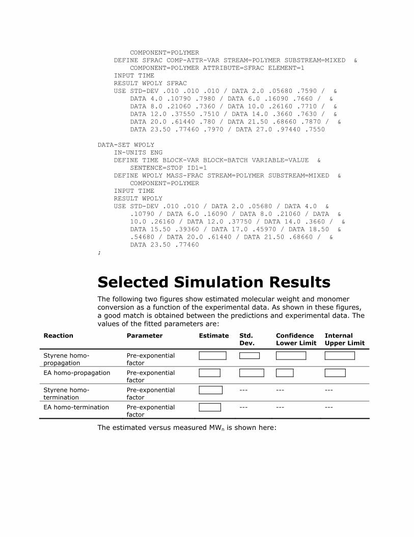
COMPONENT=POLYMER DEFINE SFRAC COMP-ATTR-VAR STREAM=POLYMER SUBSTREAM=MIXED & COMPONENT=POLYMER ATTRIBUTE=SFRAC ELEMENT=1 INPUT TIME RESULT WPOLY SFRAC USE STD-DEV .010 .010 .010 / DATA 2.0 .05680 .7590 / & DATA 4.0 .10790 .7980 / DATA 6.0 .16090 .7660 / & DATA 8.0 .21060 .7360 / DATA 10.0 .26160 .7710 / & DATA 12.0 .37550 .7510 / DATA 14.0 .3660 .7630 / & DATA 20.0 .61440 .780 / DATA 21.50 .68660 .7870 / & DATA 23.50 .77460 .7970 / DATA 27.0 .97440 .7550 DATA-SET WPOLY IN-UNITS ENG DEFINE TIME BLOCK-VAR BLOCK=BATCH VARIABLE=VALUE & SENTENCE=STOP ID1=1 DEFINE WPOLY MASS-FRAC STREAM=POLYMER SUBSTREAM=MIXED & COMPONENT=POLYMER INPUT TIME RESULT WPOLY USE STD-DEV .010 .010 / DATA 2.0 .05680 / DATA 4.0 & .10790 / DATA 6.0 .16090 / DATA 8.0 .21060 / DATA & 10.0 .26160 / DATA 12.0 .37750 / DATA 14.0 .3660 / & DATA 15.50 .39360 / DATA 17.0 .45970 / DATA 18.50 & .54680 / DATA 20.0 .61440 / DATA 21.50 .68660 / & DATA 23.50 .77460 ;
Selected Simulation Results The following two figures show estimated molecular weight and monomer conversion as a function of the experimental data. As shown in these figures, a good match is obtained between the predictions and experimental data. The values of the fitted parameters are:
Reaction Parameter Estimate Std. Dev.
Confidence Lower Limit
Internal Upper Limit
Styrene homo-propagation
Pre-exponential factor
EA homo-propagation Pre-exponential factor
Styrene homo-termination
Pre-exponential factor
--- --- ---
EA homo-termination Pre-exponential factor
--- --- ---
The estimated versus measured MWn is shown here:
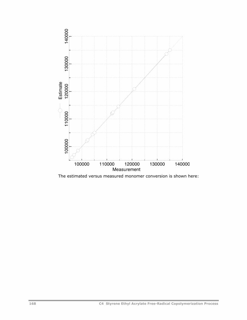
168 C4 Styrene Ethyl Acrylate Free-Radical Copolymerization Process
The estimated versus measured monomer conversion is shown here:
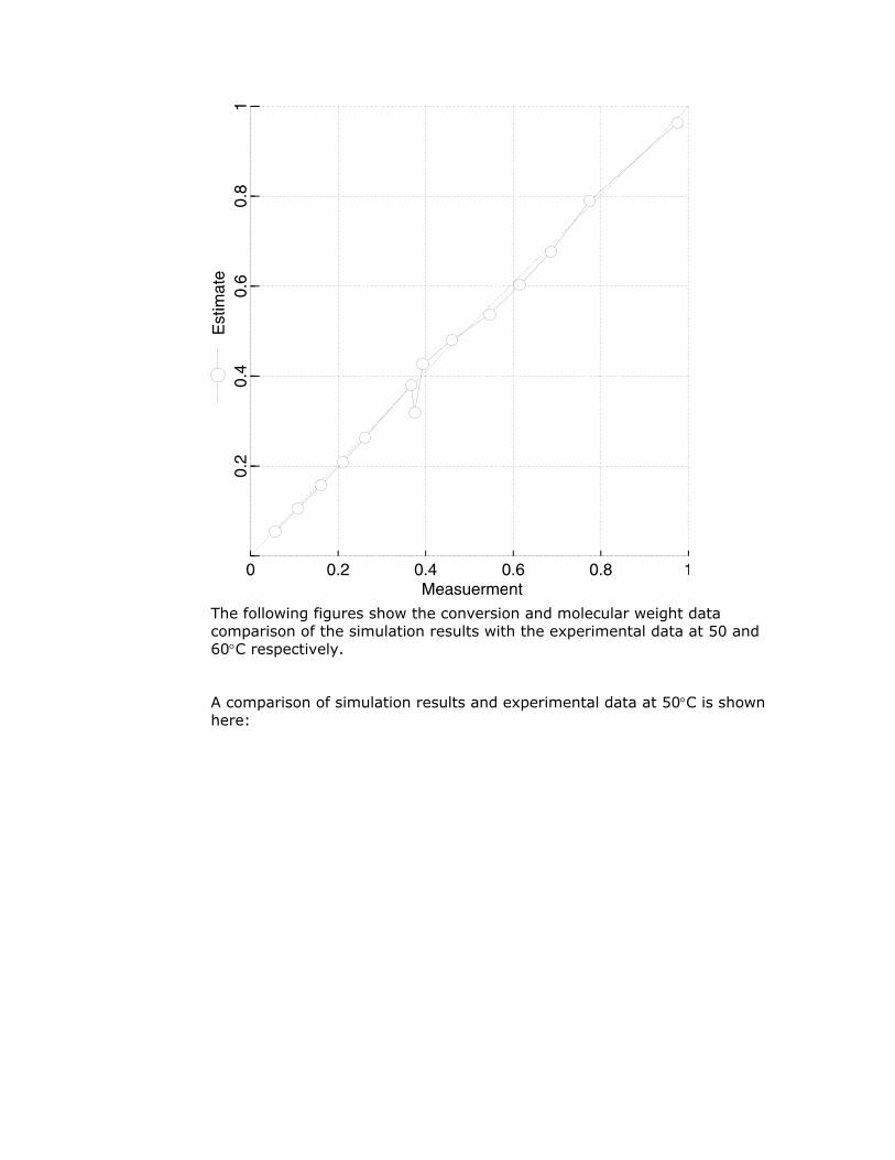
The following figures show the conversion and molecular weight data comparison of the simulation results with the experimental data at 50 and 60°C respectively.
A comparison of simulation results and experimental data at 50°C is shown here:
170 C4 Styrene Ethyl Acrylate Free-Radical Copolymerization Process
A comparison of simulation results and experimental data at 60°C is shown here:
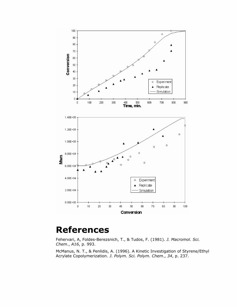
References Fehervari, A, Foldes-Berezsnich, T., & Tudos, F. (1981). J. Macromol. Sci. Chem., A16, p. 993.
McManus, N. T., & Penlidis, A. (1996). A Kinetic Investigation of Styrene/Ethyl Acrylate Copolymerization. J. Polym. Sci. Polym. Chem., 34, p. 237.
172 C5 Styrene Butadiene Emulsion Copolymerization Process
C5 Styrene Butadiene Emulsion Copolymerization Process
The styrene butadiene emulsion copolymerization process model illustrates the use of Aspen Polymers Plus to model the free-radical emulsion polymerization of styrene and butadiene in a semi-batch reactor. The model is used to examine several process parameters as a function of time: average number of radicals per particle, monomer concentration in the various phases, and monomer conversion.
About This Process In this process, the emulsion copolymerization of styrene and butadiene is carried out in a batch reactor using ammonium persulfate (APS) as the initiator, sodium lauryl sulfate (SLS) as the emulsifier and tertiary dodecyl mercaptane (TDM) as a chain transfer agent. Functionalized styrene-butadiene emulsions are used in a variety of applications such as paper coatings, carpet backings, non-wovens, etc. In addition, emulsion polymerization is the major route for the production of synthetic rubber used in the tire industries. Most styrene-butadiene rubber (SBR) latexes are manufactured in semi-batch reactors. SBR production technology is detailed by Blackley (Blackley, 1983).
In a typical semi-batch process employing in-situ seeding, the initial charge is used for the production of seed particles, with the desired particle size and particle size distribution. Usually, anionic emulsifiers and water-soluble persulfate initiators are used for particle nucleation by the micellar mechanism.
When the initial mixture is heated, the radicals generated from the initiator become surface active and enter micelles to form particles. Once the particle specifications are met, monomers and other ingredients, such as chain transfer agent, stabilizers, initiators, are continuously added to the reactor, and the particles are grown to the desired final particle size.
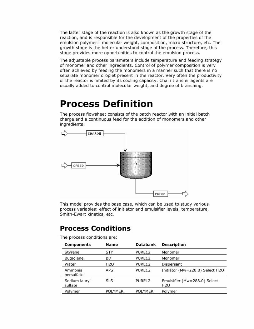
The latter stage of the reaction is also known as the growth stage of the reaction, and is responsible for the development of the properties of the emulsion polymer: molecular weight, composition, micro structure, etc. The growth stage is the better understood stage of the process. Therefore, this stage provides more opportunities to control the emulsion process.
The adjustable process parameters include temperature and feeding strategy of monomer and other ingredients. Control of polymer composition is very often achieved by feeding the monomers in a manner such that there is no separate monomer droplet present in the reactor. Very often the productivity of the reactor is limited by its cooling capacity. Chain transfer agents are usually added to control molecular weight, and degree of branching.
Process Definition The process flowsheet consists of the batch reactor with an initial batch charge and a continuous feed for the addition of monomers and other ingredients:
This model provides the base case, which can be used to study various process variables: effect of initiator and emulsifier levels, temperature, Smith-Ewart kinetics, etc.
Process Conditions The process conditions are:
Components Name Databank Description
Styrene STY PURE12 Monomer
Butadiene BD PURE12 Monomer
Water H2O PURE12 Dispersant
Ammonia persulfate
APS PURE12 Initiator (Mw=220.0) Select H2O
Sodium lauryl sulfate
SLS PURE12 Emulsifier (Mw=288.0) Select H2O
Polymer POLYMER POLYMER Polymer
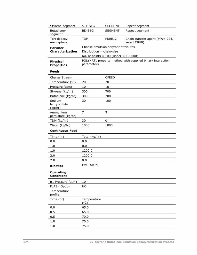
174 C5 Styrene Butadiene Emulsion Copolymerization Process
Styrene-segment STY-SEG SEGMENT Repeat segment
Butadiene-segment
BD-SEG SEGMENT Repeat segment
Tert dodecyl mercaptane
TDM PURE12 Chain transfer agent (MW= 224, select C8H8)
Polymer Characterization
Choose emulsion polymer attributes
Distribution = chain-size
No. of points = 100 (upper = 100000)
Physical Properties
POLYNRTL property method with supplied binary interaction parameters
Feeds
Charge Stream CFEED
Temperature (°C) 20 20
Pressure (atm) 10 10
Styrene (kg/hr) 300 700
Butadiene (kg/hr) 300 700
Sodium laurylsulfate (kg/hr)
30 100
Ammonium persulfate (kg/hr)
7 3
TDM (kg/hr) 30 0
Water (kg/hr) 1000 1000
Continuous Feed
Time (hr) Total (kg/hr)
0.0 0.0
1.0 0.0
1.0 1200.0
2.0 1200.0
2.0 0.0
Kinetics EMULSION
Operating Conditions
B1 Pressure (atm) 10
FLASH Option NO
Temperature profile
Time (hr) Temperature (°C)
0.0 65.0
0.5 65.0
0.5 70.0
1.0 70.0
1.0 75.0
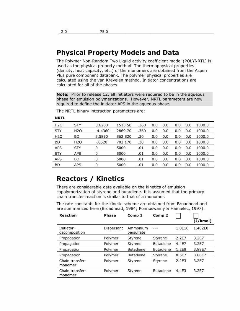
2.0 75.0
Physical Property Models and Data The Polymer Non-Random Two Liquid activity coefficient model (POLYNRTL) is used as the physical property method. The thermophysical properties (density, heat capacity, etc.) of the monomers are obtained from the Aspen Plus pure component databank. The polymer physical properties are calculated using the van Krevelen method. Initiator concentrations are calculated for all of the phases.
Note: Prior to release 12, all initiators were required to be in the aqueous phase for emulsion polymerizations. However, NRTL parameters are now required to define the initiator APS in the aqueous phase.
The NRTL binary interaction parameters are:
NRTL
H2O STY 3.6260 1513.50 .360 0.0 0.0 0.0 0.0 1000.0
STY H2O -4.4360 2869.70 .360 0.0 0.0 0.0 0.0 1000.0
H2O BD 3.5890 862.820 .30 0.0 0.0 0.0 0.0 1000.0
BD H2O -.8520 702.170 .30 0.0 0.0 0.0 0.0 1000.0
APS STY 0 5000 .01 0.0 0.0 0.0 0.0 1000.0
STY APS 0 5000 .01 0.0 0.0 0.0 0.0 1000.0
APS BD 0 5000 .01 0.0 0.0 0.0 0.0 1000.0
BD APS 0 5000 .01 0.0 0.0 0.0 0.0 1000.0
Reactors / Kinetics There are considerable data available on the kinetics of emulsion copolymerization of styrene and butadiene. It is assumed that the primary chain transfer reaction is similar to that of a monomer.
The rate constants for the kinetic scheme are obtained from Broadhead and are summarized here (Broadhead, 1984; Ponnuswamy & Hamielec, 1997):
Reaction Phase Comp 1 Comp 2
(J/kmol)
Initiator decomposition
Dispersant Ammonium persulfate
--- 1.0E16 1.402E8
Propagation Polymer Styrene Styrene 2.2E7 3.2E7
Propagation Polymer Styrene Butadiene 4.4E7 3.2E7
Propagation Polymer Butadiene Butadiene 1.2E8 3.88E7
Propagation Polymer Butadiene Styrene 8.5E7 3.88E7
Chain transfer-monomer
Polymer Styrene Styrene 2.2E3 3.2E7
Chain transfer-monomer
Polymer Styrene Butadiene 4.4E3 3.2E7
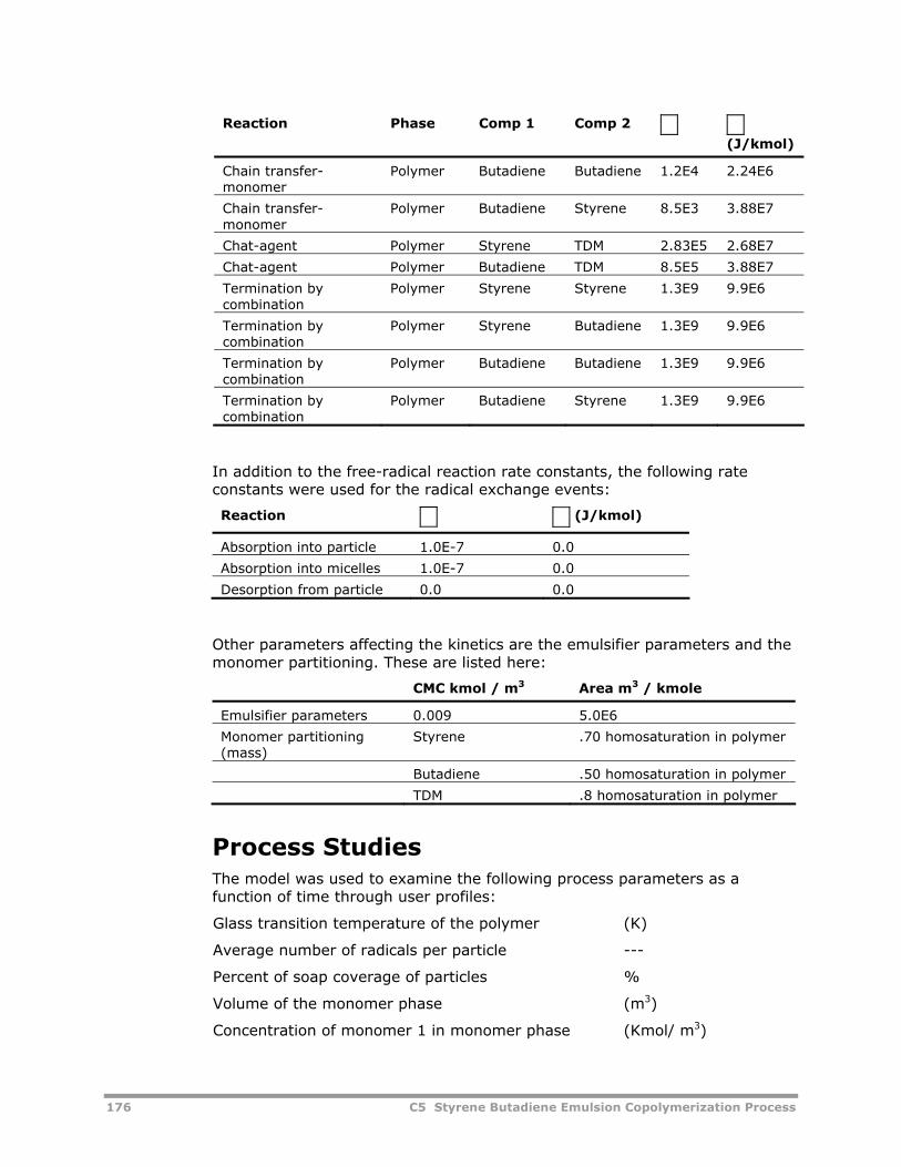
176 C5 Styrene Butadiene Emulsion Copolymerization Process
Reaction Phase Comp 1 Comp 2
(J/kmol)
Chain transfer-monomer
Polymer Butadiene Butadiene 1.2E4 2.24E6
Chain transfer-monomer
Polymer Butadiene Styrene 8.5E3 3.88E7
Chat-agent Polymer Styrene TDM 2.83E5 2.68E7
Chat-agent Polymer Butadiene TDM 8.5E5 3.88E7
Termination by combination
Polymer Styrene Styrene 1.3E9 9.9E6
Termination by combination
Polymer Styrene Butadiene 1.3E9 9.9E6
Termination by combination
Polymer Butadiene Butadiene 1.3E9 9.9E6
Termination by combination
Polymer Butadiene Styrene 1.3E9 9.9E6
In addition to the free-radical reaction rate constants, the following rate constants were used for the radical exchange events:
Reaction (J/kmol)
Absorption into particle 1.0E-7 0.0
Absorption into micelles 1.0E-7 0.0
Desorption from particle 0.0 0.0
Other parameters affecting the kinetics are the emulsifier parameters and the monomer partitioning. These are listed here:
CMC kmol / m3 Area m3 / kmole
Emulsifier parameters 0.009 5.0E6
Monomer partitioning (mass)
Styrene .70 homosaturation in polymer
Butadiene .50 homosaturation in polymer
TDM .8 homosaturation in polymer
Process Studies The model was used to examine the following process parameters as a function of time through user profiles:
Glass transition temperature of the polymer (K)
Average number of radicals per particle ---
Percent of soap coverage of particles %
Volume of the monomer phase (m3)
Concentration of monomer 1 in monomer phase (Kmol/ m3)
Concentration of monomer 2 in monomer phase (Kmol/ m3)
Volume of the aqueous phase (m3)
Concentration of the monomer 1 in aqueous phase (Kmol / m3)
Concentration of the monomer 2 in aqueous phase (Kmol / m3)
Volume of the polymer phase (m3)
Concentration of the monomer 1 in polymer phase (Kmol / m3)
Concentration of the monomer 2 in polymer phase (Kmol / m3)
Total mass conversion of monomer to polymer ---
Input Summary The input language summary for this example is shown here:
TITLE 'EMULSION COPOLYMERIZATION OF STYRENE AND BUTADIENE' IN-UNITS SI MASS-FLOW='kg/hr' PRESSURE=bar TEMPERATURE=C TIME=hr & PDROP='N/sqm' DEF-STREAMS CONVEN ALL SYS-OPTIONS TRACE=YES DESCRIPTION " THIS EXAMPLE ILLUSTRATES THE USE OF ASPEN POLYMERS PLUS TO MODEL THE COPOLYMERIZATION OF STYRENE AND BUTADIENE IN A BATCH REACTOR. " DATABANKS PURE12 / POLYMER / SEGMENT / NOASPENPCD PROP-SOURCES PURE12 / POLYMER / SEGMENT COMPONENTS H2O H2O / STY C8H8 / BD C4H6-4 / POLYMER POLYMER / STY-SEG C8H8-R / BD-SEG C4H6-R-1 / APS H2O / SLS H2O / TDM C8H8 FLOWSHEET BLOCK REACTOR IN=CHARGE CONTFEED OUT=PRODUCT PROPERTIES POLYNRTL
178 C5 Styrene Butadiene Emulsion Copolymerization Process
USER-PROPS GMRENA 1 2 1 / GMRENB 1 2 1 / GMRENC 1 2 1 / & GMREND 1 2 1 PROP-DATA MW IN-UNITS SI MASS-FLOW='kg/hr' PRESSURE=bar TEMPERATURE=C & TIME=hr PDROP='N/sqm' PROP-LIST MW PVAL APS 228.0 PVAL SLS 288.0 PVAL TDM 202.40 PROP-DATA TGVK IN-UNITS SI MASS-FLOW='kg/hr' PRESSURE=bar TEMPERATURE=C & TIME=hr PDROP='N/sqm' PROP-LIST TGVK PVAL STY-SEG 100.0 PVAL BD-SEG -54.0 PROP-DATA NRTL-1 IN-UNITS SI PROP-LIST NRTL BPVAL H2O STY 3.6260 1513.50 .360 0.0 0.0 0.0 0.0 & 1000.0 BPVAL STY H2O -4.4360 2869.70 .360 0.0 0.0 0.0 0.0 & 1000.0 BPVAL H2O BD 3.5890 862.820 .30 0.0 0.0 0.0 0.0 1000.0 BPVAL BD H2O -.8520 702.170 .30 0.0 0.0 0.0 0.0 1000.0 BPVAL APS STY 0 5000 .01 0.0 0.0 0.0 0.0 1000.000 BPVAL STY APS 0.0 5000 .01 0.0 0.0 0.0 0.0 1000.000 BPVAL APS BD 0 5000 .01 0.0 0.0 0.0 0.0 1000.000 BPVAL BD APS 0.0 5000 .01 0.0 0.0 0.0 0.0 1000.000 POLYMERS SEGMENTS STY-SEG REPEAT / BD-SEG REPEAT POLYMERS POLYMER ATTRIBUTES POLYMER SFRAC SFLOW DPN DPW PDI MWN MWW ZMOM & FMOM SMOM PSDZMOM PSDFMOM DIAV DISTRIBUTION POLYMER CHAIN-SIZE CLD NPOINTS=100 FUNCLOG=NO & UPPER=100000.0 PROP-SET PS-1 MASSFRAC SUBSTREAM=MIXED COMPS=POLYMER PHASE=L STREAM CHARGE SUBSTREAM MIXED TEMP=20.0 PRES=10.0 MASS-FLOW H2O 1000.0 / STY 300.0 / BD 300.0 / POLYMER & 0.0 / APS 7.0 / SLS 30.0 / TDM 30.0 STREAM CONTFEED SUBSTREAM MIXED TEMP=20.0 PRES=10.0 MASS-FLOW H2O 1000.0 / STY 700.0 / BD 700.0 / POLYMER & 0.0 / APS 3.0 / SLS 100.0 BLOCK REACTOR RBATCH USER-VECS NUSER-PROF=13 USERPROF ELEMENT=1 LABEL="TGAVG" UNIT-LABEL="DEG K" USERPROF ELEMENT=2 LABEL="NBAR" UNIT-LABEL="#/PARTICLE" USERPROF ELEMENT=3 LABEL="S-COVER" UNIT-LABEL="%"
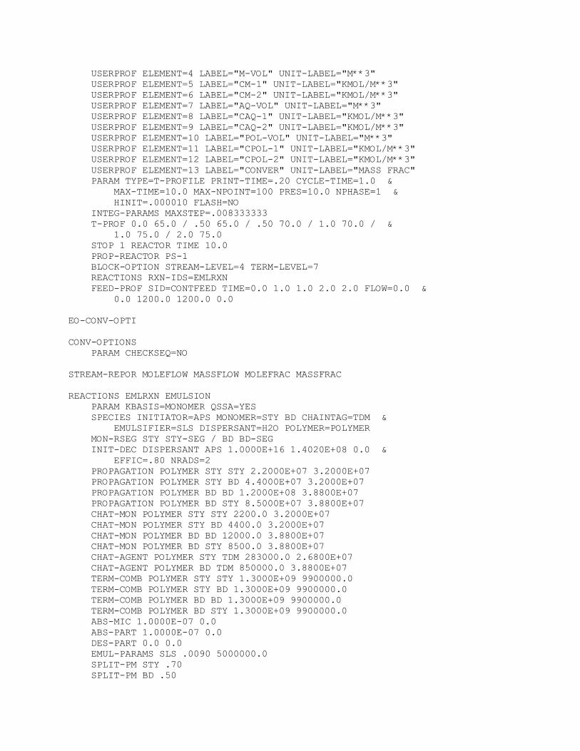
USERPROF ELEMENT=4 LABEL="M-VOL" UNIT-LABEL="M**3" USERPROF ELEMENT=5 LABEL="CM-1" UNIT-LABEL="KMOL/M**3" USERPROF ELEMENT=6 LABEL="CM-2" UNIT-LABEL="KMOL/M**3" USERPROF ELEMENT=7 LABEL="AQ-VOL" UNIT-LABEL="M**3" USERPROF ELEMENT=8 LABEL="CAQ-1" UNIT-LABEL="KMOL/M**3" USERPROF ELEMENT=9 LABEL="CAQ-2" UNIT-LABEL="KMOL/M**3" USERPROF ELEMENT=10 LABEL="POL-VOL" UNIT-LABEL="M**3" USERPROF ELEMENT=11 LABEL="CPOL-1" UNIT-LABEL="KMOL/M**3" USERPROF ELEMENT=12 LABEL="CPOL-2" UNIT-LABEL="KMOL/M**3" USERPROF ELEMENT=13 LABEL="CONVER" UNIT-LABEL="MASS FRAC" PARAM TYPE=T-PROFILE PRINT-TIME=.20 CYCLE-TIME=1.0 & MAX-TIME=10.0 MAX-NPOINT=100 PRES=10.0 NPHASE=1 & HINIT=.000010 FLASH=NO INTEG-PARAMS MAXSTEP=.008333333 T-PROF 0.0 65.0 / .50 65.0 / .50 70.0 / 1.0 70.0 / & 1.0 75.0 / 2.0 75.0 STOP 1 REACTOR TIME 10.0 PROP-REACTOR PS-1 BLOCK-OPTION STREAM-LEVEL=4 TERM-LEVEL=7 REACTIONS RXN-IDS=EMLRXN FEED-PROF SID=CONTFEED TIME=0.0 1.0 1.0 2.0 2.0 FLOW=0.0 & 0.0 1200.0 1200.0 0.0 EO-CONV-OPTI CONV-OPTIONS PARAM CHECKSEQ=NO STREAM-REPOR MOLEFLOW MASSFLOW MOLEFRAC MASSFRAC REACTIONS EMLRXN EMULSION PARAM KBASIS=MONOMER QSSA=YES SPECIES INITIATOR=APS MONOMER=STY BD CHAINTAG=TDM & EMULSIFIER=SLS DISPERSANT=H2O POLYMER=POLYMER MON-RSEG STY STY-SEG / BD BD-SEG INIT-DEC DISPERSANT APS 1.0000E+16 1.4020E+08 0.0 & EFFIC=.80 NRADS=2 PROPAGATION POLYMER STY STY 2.2000E+07 3.2000E+07 PROPAGATION POLYMER STY BD 4.4000E+07 3.2000E+07 PROPAGATION POLYMER BD BD 1.2000E+08 3.8800E+07 PROPAGATION POLYMER BD STY 8.5000E+07 3.8800E+07 CHAT-MON POLYMER STY STY 2200.0 3.2000E+07 CHAT-MON POLYMER STY BD 4400.0 3.2000E+07 CHAT-MON POLYMER BD BD 12000.0 3.8800E+07 CHAT-MON POLYMER BD STY 8500.0 3.8800E+07 CHAT-AGENT POLYMER STY TDM 283000.0 2.6800E+07 CHAT-AGENT POLYMER BD TDM 850000.0 3.8800E+07 TERM-COMB POLYMER STY STY 1.3000E+09 9900000.0 TERM-COMB POLYMER STY BD 1.3000E+09 9900000.0 TERM-COMB POLYMER BD BD 1.3000E+09 9900000.0 TERM-COMB POLYMER BD STY 1.3000E+09 9900000.0 ABS-MIC 1.0000E-07 0.0 ABS-PART 1.0000E-07 0.0 DES-PART 0.0 0.0 EMUL-PARAMS SLS .0090 5000000.0 SPLIT-PM STY .70 SPLIT-PM BD .50
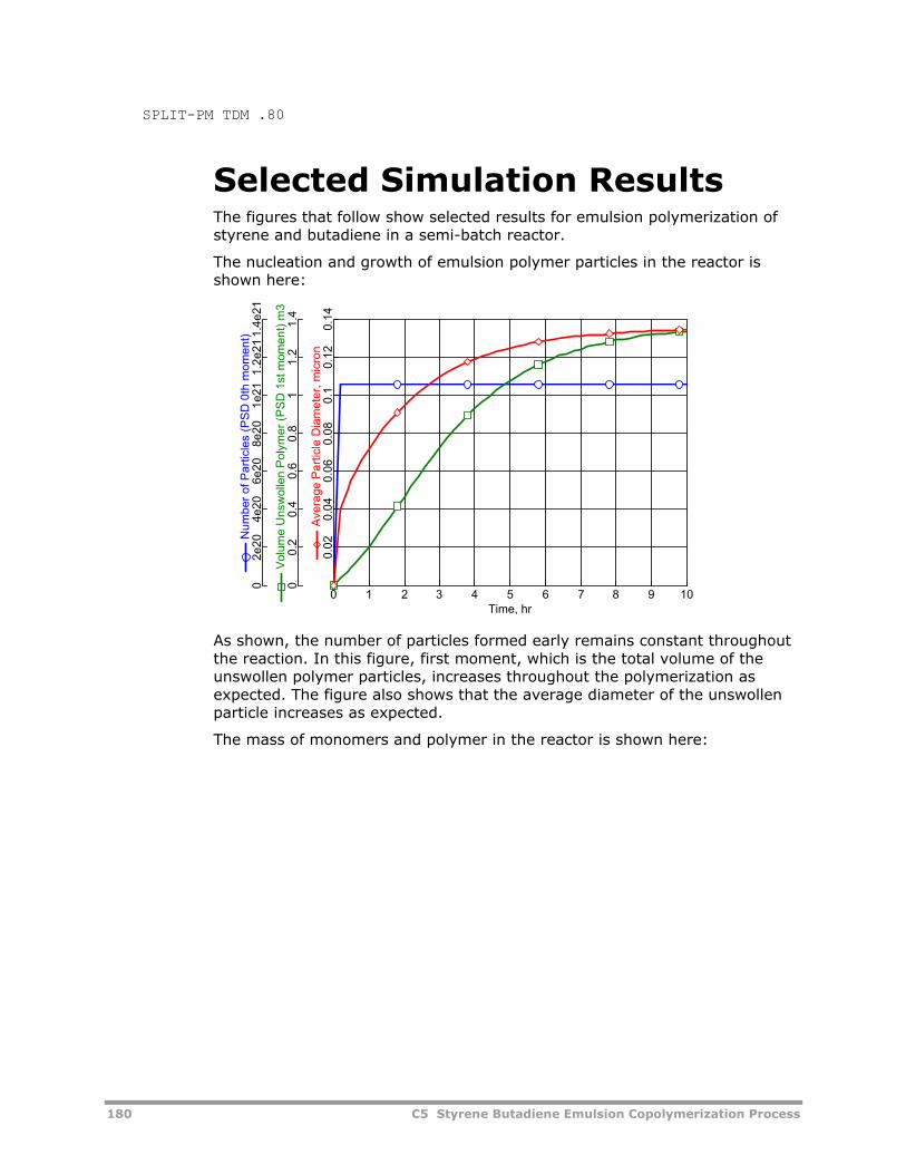
180 C5 Styrene Butadiene Emulsion Copolymerization Process
SPLIT-PM TDM .80
Selected Simulation Results The figures that follow show selected results for emulsion polymerization of styrene and butadiene in a semi-batch reactor.
The nucleation and growth of emulsion polymer particles in the reactor is shown here:
Time, hr
Ave
rage
Par
ticle
Dia
met
er, m
icro
n
Vol
ume
Uns
wol
len
Pol
ymer
(PS
D 1
st m
omen
t) m
3
Num
ber o
f Par
ticle
s (P
SD
0th
mom
ent)
0 1 2 3 4 5 6 7 8 9 10
0.02
0.04
0.06
0.08
0.1
0.12
0.14
00.
20.
40.
60.
81
1.2
1.4
02e
204e
206e
208e
201e
211.
2e21
1.4e
21
As shown, the number of particles formed early remains constant throughout the reaction. In this figure, first moment, which is the total volume of the unswollen polymer particles, increases throughout the polymerization as expected. The figure also shows that the average diameter of the unswollen particle increases as expected.
The mass of monomers and polymer in the reactor is shown here:
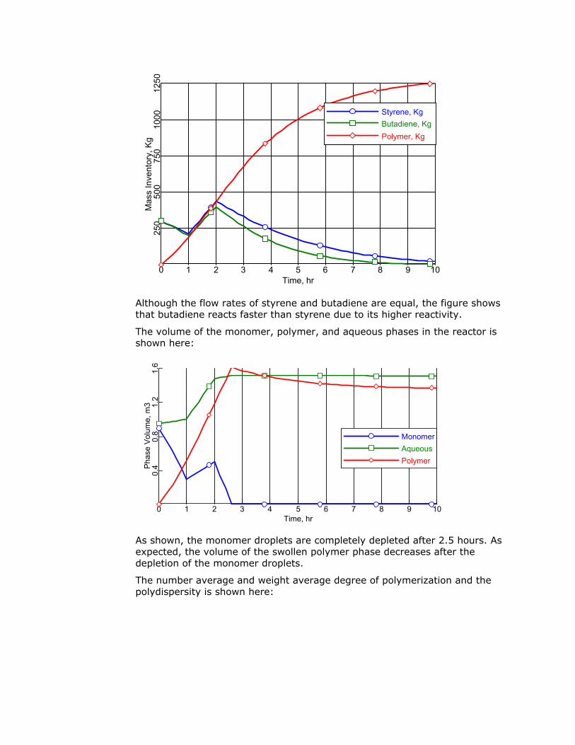
Time, hr
Mas
s In
vent
ory,
Kg
0 1 2 3 4 5 6 7 8 9 10
250
500
750
1000
1250
Styrene, KgButadiene, KgPolymer, Kg
Although the flow rates of styrene and butadiene are equal, the figure shows that butadiene reacts faster than styrene due to its higher reactivity.
The volume of the monomer, polymer, and aqueous phases in the reactor is shown here:
Time, hr
Pha
se V
olum
e, m
3
0 1 2 3 4 5 6 7 8 9 10
0.4
0.8
1.2
1.6
MonomerAqueousPolymer
As shown, the monomer droplets are completely depleted after 2.5 hours. As expected, the volume of the swollen polymer phase decreases after the depletion of the monomer droplets.
The number average and weight average degree of polymerization and the polydispersity is shown here:
182 C5 Styrene Butadiene Emulsion Copolymerization Process
Time, hr
Pol
ydis
pers
ity In
dex
Deg
ree
of P
olym
eriz
atio
n
0 1 2 3 4 5 6 7 8 9 10
22.
53
3.5
4
010
0020
0030
0040
0050
0060
00
DPNDPWPDI
The composition of the polymer is shown here:
Time, hr
Mol
e Fr
actio
n, S
FRA
C
0 1 2 3 4 5 6 7 8 9 10
0.1
0.2
0.3
0.4
0.5
0.6
0.7
0.8
StyreneButadiene
As expected, the composition of the reactive butadiene monomer in the polymer is higher in comparison to styrene.
The chain length distribution is shown here:
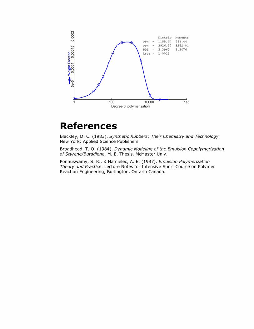
Degree of polymerization
Wei
ght F
ract
ion
1 100 10000 1e6
5e-5
0.00
010.
0001
50.
0002
Distrib MomentsDPN = 1155.97 968.44DPW = 3926.32 3242.01PDI = 3.3965 3.3476Area = 1.0021
References Blackley, D. C. (1983). Synthetic Rubbers: Their Chemistry and Technology. New York: Applied Science Publishers.
Broadhead, T. O. (1984). Dynamic Modeling of the Emulsion Copolymerization of Styrene/Butadiene. M. E. Thesis, McMaster Univ.
Ponnuswamy, S. R., & Hamielec, A. E. (1997). Emulsion Polymerization Theory and Practice. Lecture Notes for Intensive Short Course on Polymer Reaction Engineering, Burlington, Ontario Canada.
184 C6 Styrene Butadiene Ionic Polymerization Processes
C6 Styrene Butadiene Ionic Polymerization Processes
The styrene butadiene rubber (SBR) ionic solution process model illustrates the use of Aspen Polymers Plus to model an anionic polymerization of styrene and butadiene. The model describes the production of tapered block copolymer using a batch reactor.
About This Process Block copolymers of styrene and butadiene are formed by living anionic polymerization initiated by alkyllithiums. These monomers can be polymerized over a wide range of useful temperatures from room temperature to elevated temperatures (100°C). Adding alkyllithium initiator to styrene and butadiene in hydrocarbon solution produces a copolymer containing long polybutadiene and polystyrene blocks (tapered block copolymers).
Although styrene homo-polymerizes more rapidly than butadiene with alkyllithiums in hydrocarbon solution, it does not polymerize first in the mixture. Butadiene is incorporated with a small amount of styrene into the copolymer first, and only then is the residual styrene free to form blocks by homopolymerization onto the polybutadienyllithium. Because of the stability of “living” nature of the allylic lithium end group, butadiene-styrene copolymers of widely different structures and properties can be prepared. The SBR copolymer can either be a random, tapered block, or di/tri-block copolymer.
The solvent influences the reactivity ratios of styrene and butadiene. The solvents change the overall rates while the general shape of the batch polymerization curves remains the same. The reactivity ratios
( ) are a strong function of the solvent. For styrene (s)
and butadiene (b) monomers in cyclohexane solvent, the reactivity ratio, rb, is about 50 times larger than rs, and these rate constants determine what type of copolymer will be formed.
If a mixture of styrene and butadiene is polymerized using alkyllithium initiator and cyclohexane solvent with the above kinetics in a batch reactor,
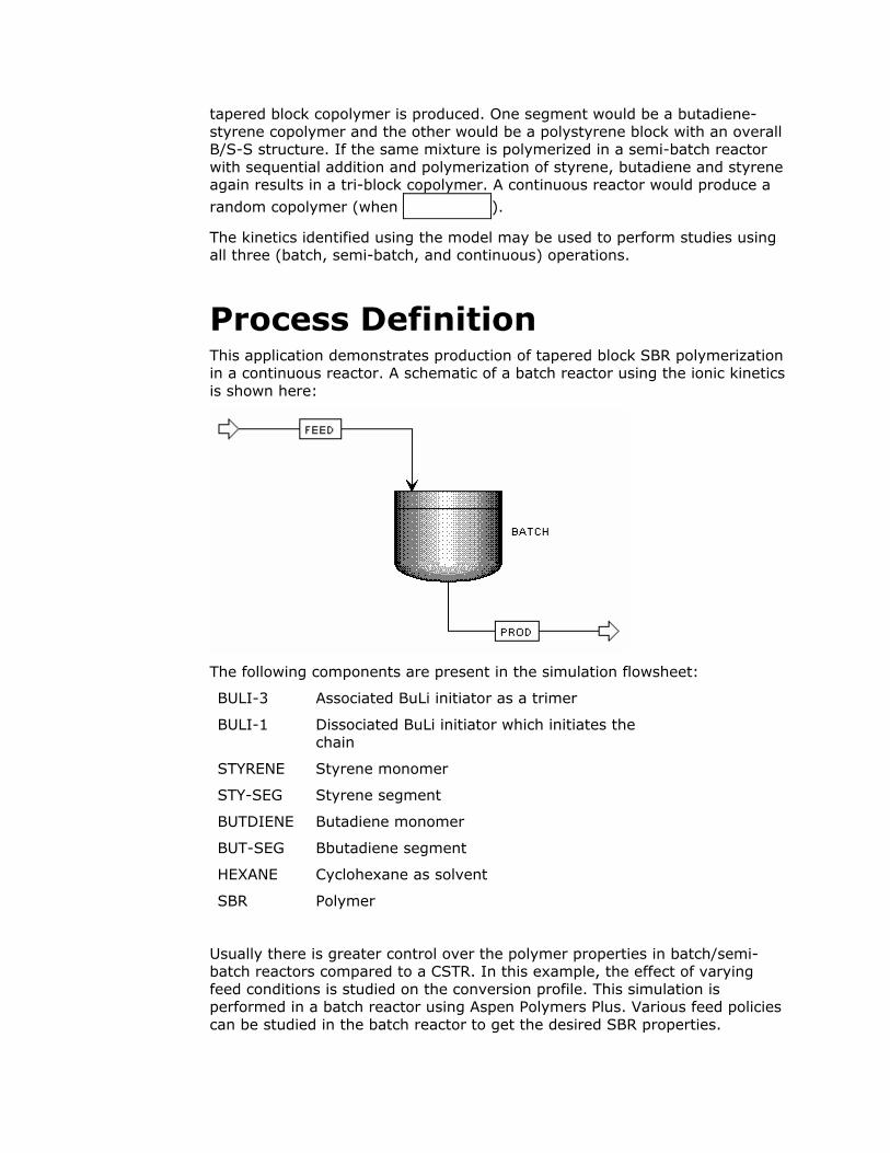
tapered block copolymer is produced. One segment would be a butadiene-styrene copolymer and the other would be a polystyrene block with an overall B/S-S structure. If the same mixture is polymerized in a semi-batch reactor with sequential addition and polymerization of styrene, butadiene and styrene again results in a tri-block copolymer. A continuous reactor would produce a
random copolymer (when ).
The kinetics identified using the model may be used to perform studies using all three (batch, semi-batch, and continuous) operations.
Process Definition This application demonstrates production of tapered block SBR polymerization in a continuous reactor. A schematic of a batch reactor using the ionic kinetics is shown here:
The following components are present in the simulation flowsheet:
BULI-3 Associated BuLi initiator as a trimer
BULI-1 Dissociated BuLi initiator which initiates the chain
STYRENE Styrene monomer
STY-SEG Styrene segment
BUTDIENE Butadiene monomer
BUT-SEG Bbutadiene segment
HEXANE Cyclohexane as solvent
SBR Polymer
Usually there is greater control over the polymer properties in batch/semi-batch reactors compared to a CSTR. In this example, the effect of varying feed conditions is studied on the conversion profile. This simulation is performed in a batch reactor using Aspen Polymers Plus. Various feed policies can be studied in the batch reactor to get the desired SBR properties.
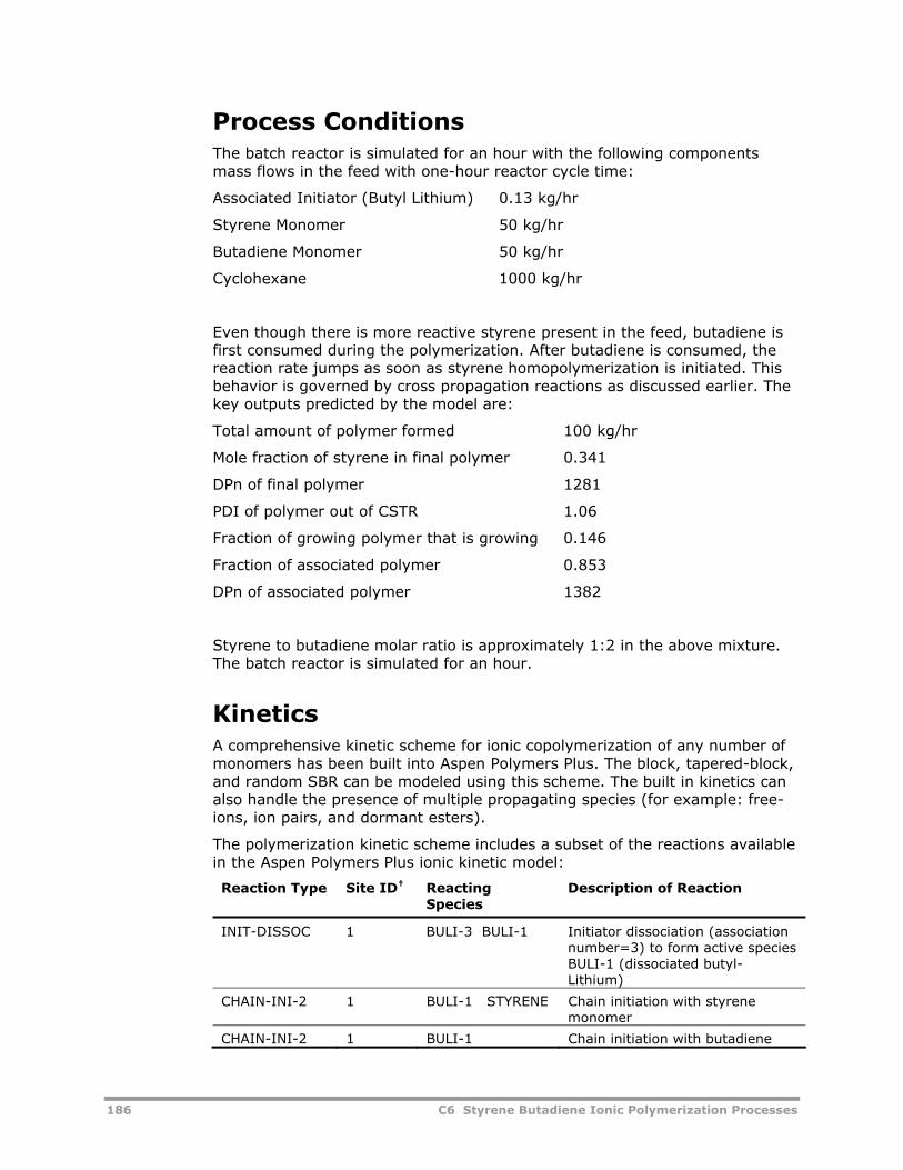
186 C6 Styrene Butadiene Ionic Polymerization Processes
Process Conditions The batch reactor is simulated for an hour with the following components mass flows in the feed with one-hour reactor cycle time:
Associated Initiator (Butyl Lithium) 0.13 kg/hr
Styrene Monomer 50 kg/hr
Butadiene Monomer 50 kg/hr
Cyclohexane 1000 kg/hr
Even though there is more reactive styrene present in the feed, butadiene is first consumed during the polymerization. After butadiene is consumed, the reaction rate jumps as soon as styrene homopolymerization is initiated. This behavior is governed by cross propagation reactions as discussed earlier. The key outputs predicted by the model are:
Total amount of polymer formed 100 kg/hr
Mole fraction of styrene in final polymer 0.341
DPn of final polymer 1281
PDI of polymer out of CSTR 1.06
Fraction of growing polymer that is growing 0.146
Fraction of associated polymer 0.853
DPn of associated polymer 1382
Styrene to butadiene molar ratio is approximately 1:2 in the above mixture. The batch reactor is simulated for an hour.
Kinetics A comprehensive kinetic scheme for ionic copolymerization of any number of monomers has been built into Aspen Polymers Plus. The block, tapered-block, and random SBR can be modeled using this scheme. The built in kinetics can also handle the presence of multiple propagating species (for example: free-ions, ion pairs, and dormant esters).
The polymerization kinetic scheme includes a subset of the reactions available in the Aspen Polymers Plus ionic kinetic model:
Reaction Type Site ID† Reacting Species
Description of Reaction
INIT-DISSOC 1 BULI-3 BULI-1 Initiator dissociation (association number=3) to form active species BULI-1 (dissociated butyl-Lithium)
CHAIN-INI-2 1 BULI-1 STYRENE Chain initiation with styrene monomer
CHAIN-INI-2 1 BULI-1 Chain initiation with butadiene
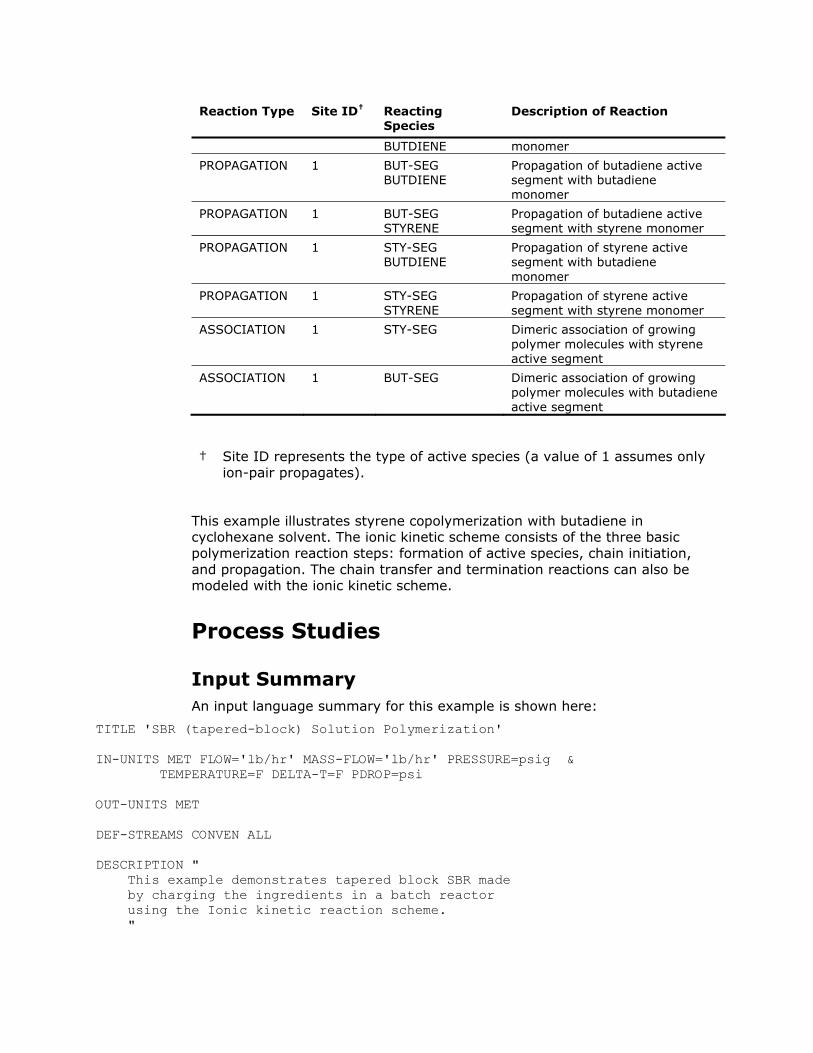
Reaction Type Site ID† Reacting Species
Description of Reaction
BUTDIENE monomer
PROPAGATION 1 BUT-SEG BUTDIENE
Propagation of butadiene active segment with butadiene monomer
PROPAGATION 1 BUT-SEG STYRENE
Propagation of butadiene active segment with styrene monomer
PROPAGATION 1 STY-SEG BUTDIENE
Propagation of styrene active segment with butadiene monomer
PROPAGATION 1 STY-SEG STYRENE
Propagation of styrene active segment with styrene monomer
ASSOCIATION 1 STY-SEG Dimeric association of growing polymer molecules with styrene active segment
ASSOCIATION 1 BUT-SEG Dimeric association of growing polymer molecules with butadiene active segment
† Site ID represents the type of active species (a value of 1 assumes only ion-pair propagates).
This example illustrates styrene copolymerization with butadiene in cyclohexane solvent. The ionic kinetic scheme consists of the three basic polymerization reaction steps: formation of active species, chain initiation, and propagation. The chain transfer and termination reactions can also be modeled with the ionic kinetic scheme.
Process Studies
Input Summary An input language summary for this example is shown here:
TITLE 'SBR (tapered-block) Solution Polymerization' IN-UNITS MET FLOW='lb/hr' MASS-FLOW='lb/hr' PRESSURE=psig & TEMPERATURE=F DELTA-T=F PDROP=psi OUT-UNITS MET DEF-STREAMS CONVEN ALL DESCRIPTION " This example demonstrates tapered block SBR made by charging the ingredients in a batch reactor using the Ionic kinetic reaction scheme. "
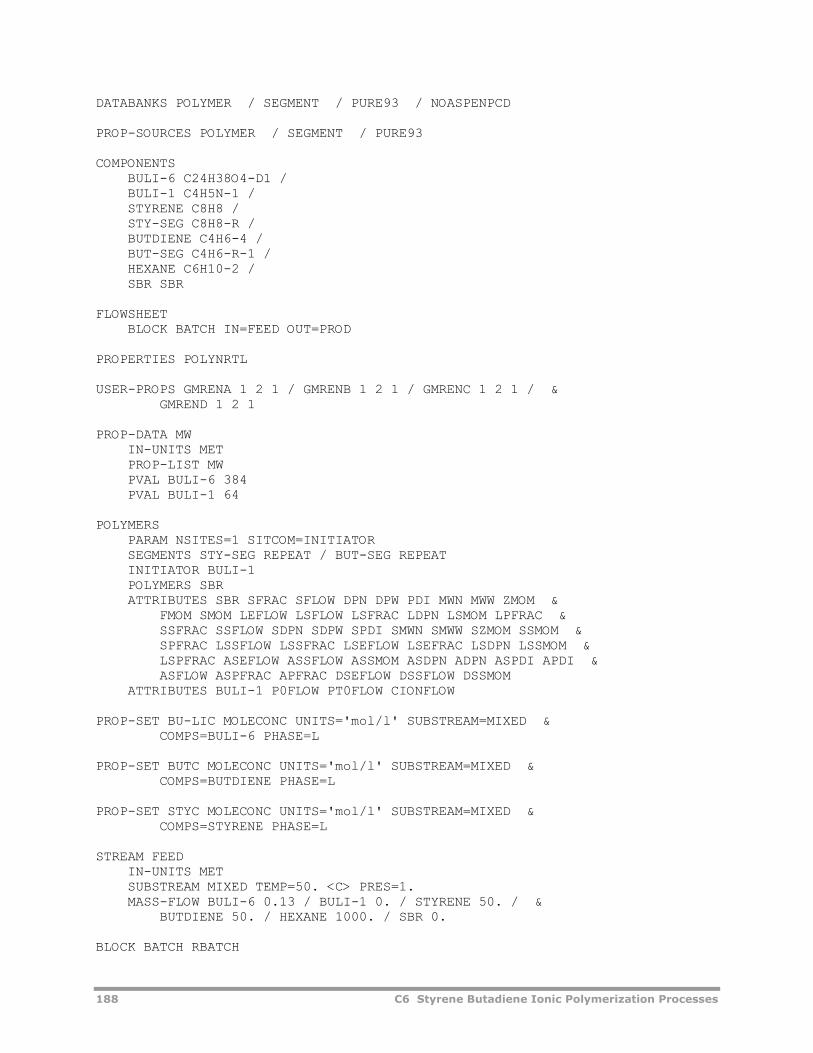
188 C6 Styrene Butadiene Ionic Polymerization Processes
DATABANKS POLYMER / SEGMENT / PURE93 / NOASPENPCD PROP-SOURCES POLYMER / SEGMENT / PURE93 COMPONENTS BULI-6 C24H38O4-D1 / BULI-1 C4H5N-1 / STYRENE C8H8 / STY-SEG C8H8-R / BUTDIENE C4H6-4 / BUT-SEG C4H6-R-1 / HEXANE C6H10-2 / SBR SBR FLOWSHEET BLOCK BATCH IN=FEED OUT=PROD PROPERTIES POLYNRTL USER-PROPS GMRENA 1 2 1 / GMRENB 1 2 1 / GMRENC 1 2 1 / & GMREND 1 2 1 PROP-DATA MW IN-UNITS MET PROP-LIST MW PVAL BULI-6 384 PVAL BULI-1 64 POLYMERS PARAM NSITES=1 SITCOM=INITIATOR SEGMENTS STY-SEG REPEAT / BUT-SEG REPEAT INITIATOR BULI-1 POLYMERS SBR ATTRIBUTES SBR SFRAC SFLOW DPN DPW PDI MWN MWW ZMOM & FMOM SMOM LEFLOW LSFLOW LSFRAC LDPN LSMOM LPFRAC & SSFRAC SSFLOW SDPN SDPW SPDI SMWN SMWW SZMOM SSMOM & SPFRAC LSSFLOW LSSFRAC LSEFLOW LSEFRAC LSDPN LSSMOM & LSPFRAC ASEFLOW ASSFLOW ASSMOM ASDPN ADPN ASPDI APDI & ASFLOW ASPFRAC APFRAC DSEFLOW DSSFLOW DSSMOM ATTRIBUTES BULI-1 P0FLOW PT0FLOW CIONFLOW PROP-SET BU-LIC MOLECONC UNITS='mol/l' SUBSTREAM=MIXED & COMPS=BULI-6 PHASE=L PROP-SET BUTC MOLECONC UNITS='mol/l' SUBSTREAM=MIXED & COMPS=BUTDIENE PHASE=L PROP-SET STYC MOLECONC UNITS='mol/l' SUBSTREAM=MIXED & COMPS=STYRENE PHASE=L STREAM FEED IN-UNITS MET SUBSTREAM MIXED TEMP=50. <C> PRES=1. MASS-FLOW BULI-6 0.13 / BULI-1 0. / STYRENE 50. / & BUTDIENE 50. / HEXANE 1000. / SBR 0. BLOCK BATCH RBATCH
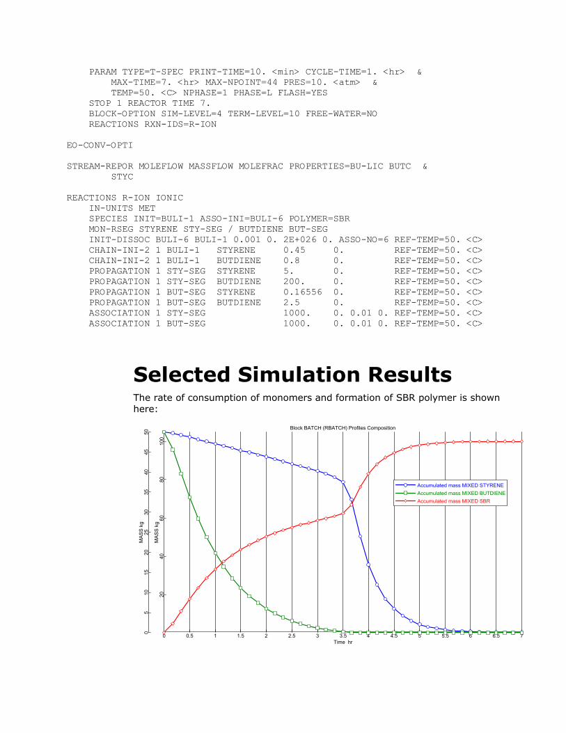
PARAM TYPE=T-SPEC PRINT-TIME=10. <min> CYCLE-TIME=1. <hr> & MAX-TIME=7. <hr> MAX-NPOINT=44 PRES=10. <atm> & TEMP=50. <C> NPHASE=1 PHASE=L FLASH=YES STOP 1 REACTOR TIME 7. BLOCK-OPTION SIM-LEVEL=4 TERM-LEVEL=10 FREE-WATER=NO REACTIONS RXN-IDS=R-ION EO-CONV-OPTI STREAM-REPOR MOLEFLOW MASSFLOW MOLEFRAC PROPERTIES=BU-LIC BUTC & STYC REACTIONS R-ION IONIC IN-UNITS MET SPECIES INIT=BULI-1 ASSO-INI=BULI-6 POLYMER=SBR MON-RSEG STYRENE STY-SEG / BUTDIENE BUT-SEG INIT-DISSOC BULI-6 BULI-1 0.001 0. 2E+026 0. ASSO-NO=6 REF-TEMP=50. <C> CHAIN-INI-2 1 BULI-1 STYRENE 0.45 0. REF-TEMP=50. <C> CHAIN-INI-2 1 BULI-1 BUTDIENE 0.8 0. REF-TEMP=50. <C> PROPAGATION 1 STY-SEG STYRENE 5. 0. REF-TEMP=50. <C> PROPAGATION 1 STY-SEG BUTDIENE 200. 0. REF-TEMP=50. <C> PROPAGATION 1 BUT-SEG STYRENE 0.16556 0. REF-TEMP=50. <C> PROPAGATION 1 BUT-SEG BUTDIENE 2.5 0. REF-TEMP=50. <C> ASSOCIATION 1 STY-SEG 1000. 0. 0.01 0. REF-TEMP=50. <C> ASSOCIATION 1 BUT-SEG 1000. 0. 0.01 0. REF-TEMP=50. <C>
Selected Simulation Results The rate of consumption of monomers and formation of SBR polymer is shown here:
Block BATCH (RBATCH) Profiles Composition
Time hr
MAS
S kg
MAS
S kg
0 0.5 1 1.5 2 2.5 3 3.5 4 4.5 5 5.5 6 6.5 7
2040
6080
100
05
1015
2025
3035
4045
50
Accumulated mass MIXED STYRENEAccumulated mass MIXED BUTDIENEAccumulated mass MIXED SBR
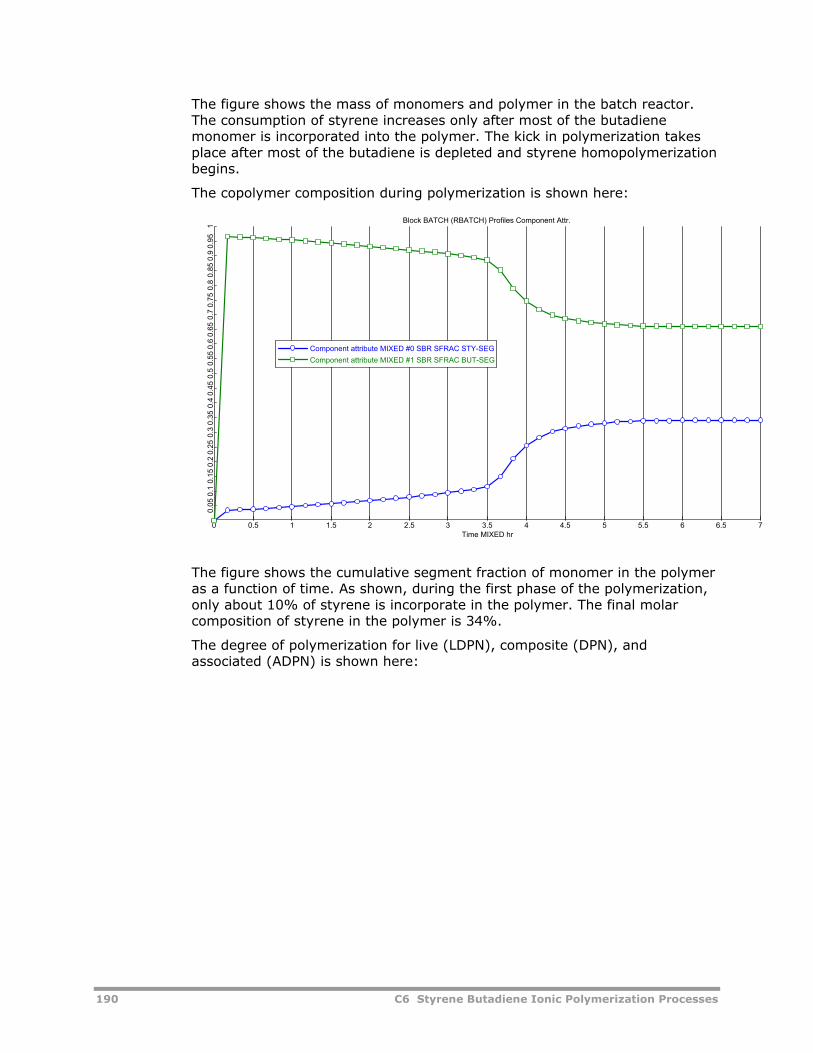
190 C6 Styrene Butadiene Ionic Polymerization Processes
The figure shows the mass of monomers and polymer in the batch reactor. The consumption of styrene increases only after most of the butadiene monomer is incorporated into the polymer. The kick in polymerization takes place after most of the butadiene is depleted and styrene homopolymerization begins.
The copolymer composition during polymerization is shown here:
Block BATCH (RBATCH) Profiles Component Attr.
Time MIXED hr
0 0.5 1 1.5 2 2.5 3 3.5 4 4.5 5 5.5 6 6.5 7
0.05
0.1
0.15
0.2
0.25
0.3
0.35
0.4
0.45
0.5
0.55
0.6
0.65
0.7
0.75
0.8
0.85
0.9
0.95
1
Component attribute MIXED #0 SBR SFRAC STY-SEGComponent attribute MIXED #1 SBR SFRAC BUT-SEG
The figure shows the cumulative segment fraction of monomer in the polymer as a function of time. As shown, during the first phase of the polymerization, only about 10% of styrene is incorporate in the polymer. The final molar composition of styrene in the polymer is 34%.
The degree of polymerization for live (LDPN), composite (DPN), and associated (ADPN) is shown here:
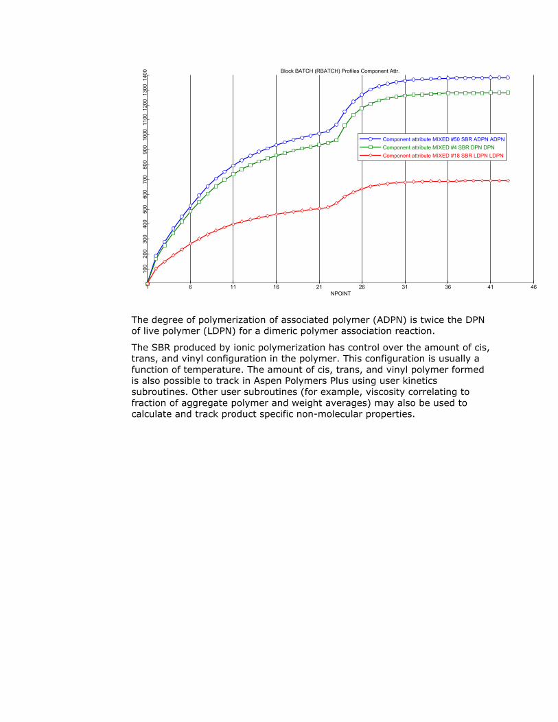
Block BATCH (RBATCH) Profiles Component Attr.
NPOINT
1 6 11 16 21 26 31 36 41 46
100
200
300
400
500
600
700
800
900
1000
1100
1200
1300
1400
Component attribute MIXED #50 SBR ADPN ADPNComponent attribute MIXED #4 SBR DPN DPNComponent attribute MIXED #18 SBR LDPN LDPN
The degree of polymerization of associated polymer (ADPN) is twice the DPN of live polymer (LDPN) for a dimeric polymer association reaction.
The SBR produced by ionic polymerization has control over the amount of cis, trans, and vinyl configuration in the polymer. This configuration is usually a function of temperature. The amount of cis, trans, and vinyl polymer formed is also possible to track in Aspen Polymers Plus using user kinetics subroutines. Other user subroutines (for example, viscosity correlating to fraction of aggregate polymer and weight averages) may also be used to calculate and track product specific non-molecular properties.
192 C7 High-Density Polyethylene High Temperature Solution Process
C7 High-Density Polyethylene High Temperature Solution Process
The HDPE high temperature solution process model illustrates the use of Aspen Polymers Plus to model a Ziegler-Natta solution polymerization of ethylene. The model is used to study the effect of feed flow rate on conversion and polymer properties, and to study the effect of hydrogen concentration on melt index and polydispersity index.
About This Process Polyethylene is the largest synthetic commodity polymer. It is widely used throughout the world due to its versatile physical and chemical properties. The current worldwide capacity for polyethylene is over 30 million tons and the average annual rate of capacity increase is 5-8%. The commercial production of polyethylene is done in continuous processes, gas-phase processes, slurry processes, or solution processes using highly active Ziegler-Natta catalysts such as titanium supported catalysts.
Aspen Polymers Plus has been used to model the high temperature solution process for polyethylene using a Ziegler-Natta catalyst. Ziegler-Natta catalysts are multi-site catalysts containing different site types, with each type having different reactivities. For this reason, each site type produces a polymer with distinct molecular weight. As a result, the composite polymer has a broad molecular weight distribution.
The Ziegler-Natta model in Aspen Polymers Plus takes into account the important reactions found in this chemistry, including site activation, chain initiation, chain propagation, chain transfer, site deactivation, site inhibition, branching reactions, etc. The model is quite flexible and can be configured for homopolymerization or copolymerization with any number of monomers. Users can also specify any number of site types for the catalyst. The model predicts the various polymer properties, such as molecular weight,
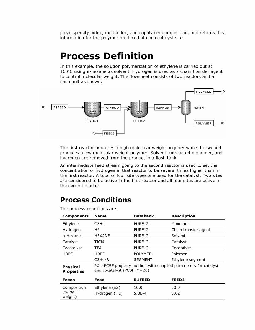
polydispersity index, melt index, and copolymer composition, and returns this information for the polymer produced at each catalyst site.
Process Definition In this example, the solution polymerization of ethylene is carried out at 160°C using n-hexane as solvent. Hydrogen is used as a chain transfer agent to control molecular weight. The flowsheet consists of two reactors and a flash unit as shown:
The first reactor produces a high molecular weight polymer while the second produces a low molecular weight polymer. Solvent, unreacted monomer, and hydrogen are removed from the product in a flash tank.
An intermediate feed stream going to the second reactor is used to set the concentration of hydrogen in that reactor to be several times higher than in the first reactor. A total of four site types are used for the catalyst. Two sites are considered to be active in the first reactor and all four sites are active in the second reactor.
Process Conditions The process conditions are:
Components Name Databank Description
Ethylene C2H4 PURE12 Monomer
Hydrogen H2 PURE12 Chain transfer agent
n-Hexane HEXANE PURE12 Solvent
Catalyst TICl4 PURE12 Catalyst
Cocatalyst TEA PURE12 Cocatalyst
HDPE HDPE
C2H4-R
POLYMER
SEGMENT
Polymer
Ethylene segment
Physical Properties
POLYPCSF property method with supplied parameters for catalyst and cocatalyst (PCSFTM=20)
Feeds Feed R1FEED FEED2
Composition (% by weight)
Ethylene (E2)
Hydrogen (H2)
10.0
5.0E-4
20.0
0.02
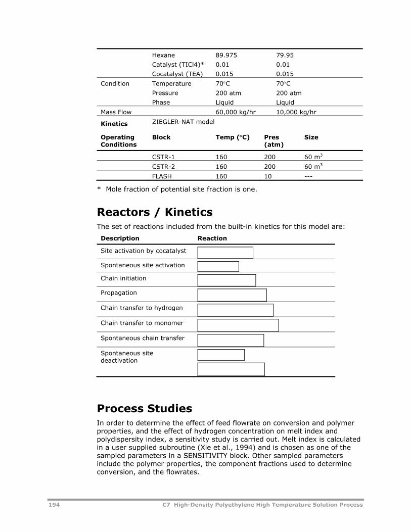
194 C7 High-Density Polyethylene High Temperature Solution Process
Hexane
Catalyst (TICl4)*
Cocatalyst (TEA)
89.975
0.01
0.015
79.95
0.01
0.015
Condition Temperature
Pressure
Phase
70°C
200 atm
Liquid
70°C
200 atm
Liquid
Mass Flow 60,000 kg/hr 10,000 kg/hr
Kinetics ZIEGLER-NAT model
Operating Conditions
Block Temp (°C) Pres (atm)
Size
CSTR-1 160 200 60 m3
CSTR-2 160 200 60 m3
FLASH 160 10 ---
* Mole fraction of potential site fraction is one.
Reactors / Kinetics The set of reactions included from the built-in kinetics for this model are:
Description Reaction
Site activation by cocatalyst
Spontaneous site activation
Chain initiation
Propagation
Chain transfer to hydrogen
Chain transfer to monomer
Spontaneous chain transfer
Spontaneous site deactivation
Process Studies In order to determine the effect of feed flowrate on conversion and polymer properties, and the effect of hydrogen concentration on melt index and polydispersity index, a sensitivity study is carried out. Melt index is calculated in a user supplied subroutine (Xie et al., 1994) and is chosen as one of the sampled parameters in a SENSITIVITY block. Other sampled parameters include the polymer properties, the component fractions used to determine conversion, and the flowrates.
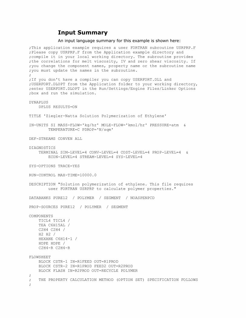
Input Summary An input language summary for this example is shown here:
;This application example requires a user FORTRAN subroutine USRPRP.F ;Please copy USRPRP.F from the Application example directory and ;compile it in your local working directory. The subroutine provides ;the correlations for melt viscosity, IV and zero shear viscosity. If ;you change the component names, property name or the subroutine name ;you must update the names in the subroutine. ; ;If you don't have a compiler you can copy USERFORT.DLL and ;USERFORT.DLOPT from the Application folder to your working directory, ;enter USERFORT.DLOPT in the Run/Settings/Engine Files/Linker Options ;box and run the simulation. DYNAPLUS DPLUS RESULTS=ON TITLE 'Ziegler-Natta Solution Polymerization of Ethylene' IN-UNITS SI MASS-FLOW='kg/hr' MOLE-FLOW='kmol/hr' PRESSURE=atm & TEMPERATURE=C PDROP='N/sqm' DEF-STREAMS CONVEN ALL DIAGNOSTICS TERMINAL SIM-LEVEL=4 CONV-LEVEL=4 COST-LEVEL=4 PROP-LEVEL=4 & ECON-LEVEL=4 STREAM-LEVEL=4 SYS-LEVEL=4 SYS-OPTIONS TRACE=YES RUN-CONTROL MAX-TIME=10000.0 DESCRIPTION "Solution polymerization of ethylene. This file requires user FORTRAN USRPRP to calculate polymer properties." DATABANKS PURE12 / POLYMER / SEGMENT / NOASPENPCD PROP-SOURCES PURE12 / POLYMER / SEGMENT COMPONENTS TICL4 TICL4 / TEA C6H15AL / C2H4 C2H4 / H2 H2 / HEXANE C6H14-1 / HDPE HDPE / C2H4-R C2H4-R FLOWSHEET BLOCK CSTR-1 IN=R1FEED OUT=R1PROD BLOCK CSTR-2 IN=R1PROD FEED2 OUT=R2PROD BLOCK FLASH IN=R2PROD OUT=RECYCLE POLYMER ; ; THE PROPERTY CALCULATION METHOD (OPTION SET) SPECIFICATION FOLLOWS ;
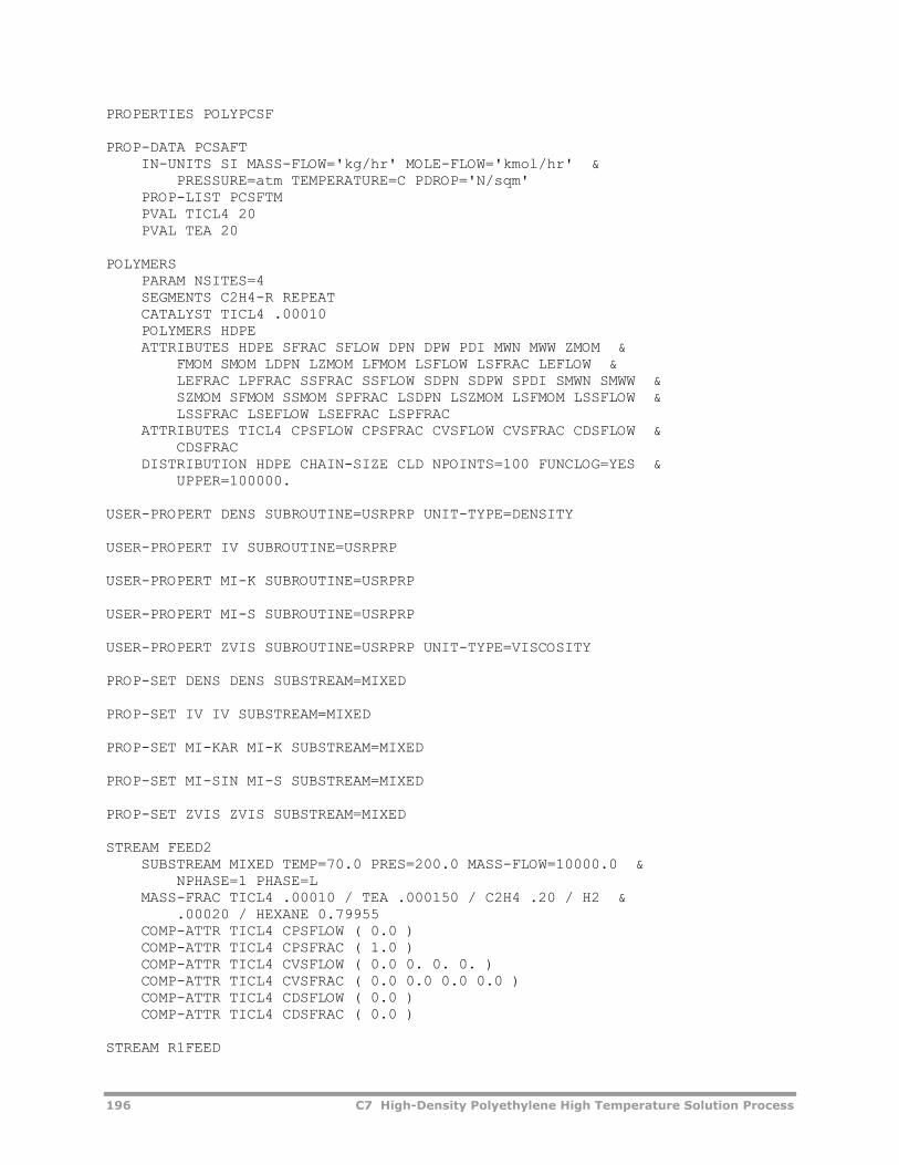
196 C7 High-Density Polyethylene High Temperature Solution Process
PROPERTIES POLYPCSF PROP-DATA PCSAFT IN-UNITS SI MASS-FLOW='kg/hr' MOLE-FLOW='kmol/hr' & PRESSURE=atm TEMPERATURE=C PDROP='N/sqm' PROP-LIST PCSFTM PVAL TICL4 20 PVAL TEA 20 POLYMERS PARAM NSITES=4 SEGMENTS C2H4-R REPEAT CATALYST TICL4 .00010 POLYMERS HDPE ATTRIBUTES HDPE SFRAC SFLOW DPN DPW PDI MWN MWW ZMOM & FMOM SMOM LDPN LZMOM LFMOM LSFLOW LSFRAC LEFLOW & LEFRAC LPFRAC SSFRAC SSFLOW SDPN SDPW SPDI SMWN SMWW & SZMOM SFMOM SSMOM SPFRAC LSDPN LSZMOM LSFMOM LSSFLOW & LSSFRAC LSEFLOW LSEFRAC LSPFRAC ATTRIBUTES TICL4 CPSFLOW CPSFRAC CVSFLOW CVSFRAC CDSFLOW & CDSFRAC DISTRIBUTION HDPE CHAIN-SIZE CLD NPOINTS=100 FUNCLOG=YES & UPPER=100000. USER-PROPERT DENS SUBROUTINE=USRPRP UNIT-TYPE=DENSITY USER-PROPERT IV SUBROUTINE=USRPRP USER-PROPERT MI-K SUBROUTINE=USRPRP USER-PROPERT MI-S SUBROUTINE=USRPRP USER-PROPERT ZVIS SUBROUTINE=USRPRP UNIT-TYPE=VISCOSITY PROP-SET DENS DENS SUBSTREAM=MIXED PROP-SET IV IV SUBSTREAM=MIXED PROP-SET MI-KAR MI-K SUBSTREAM=MIXED PROP-SET MI-SIN MI-S SUBSTREAM=MIXED PROP-SET ZVIS ZVIS SUBSTREAM=MIXED STREAM FEED2 SUBSTREAM MIXED TEMP=70.0 PRES=200.0 MASS-FLOW=10000.0 & NPHASE=1 PHASE=L MASS-FRAC TICL4 .00010 / TEA .000150 / C2H4 .20 / H2 & .00020 / HEXANE 0.79955 COMP-ATTR TICL4 CPSFLOW ( 0.0 ) COMP-ATTR TICL4 CPSFRAC ( 1.0 ) COMP-ATTR TICL4 CVSFLOW ( 0.0 0. 0. 0. ) COMP-ATTR TICL4 CVSFRAC ( 0.0 0.0 0.0 0.0 ) COMP-ATTR TICL4 CDSFLOW ( 0.0 ) COMP-ATTR TICL4 CDSFRAC ( 0.0 ) STREAM R1FEED
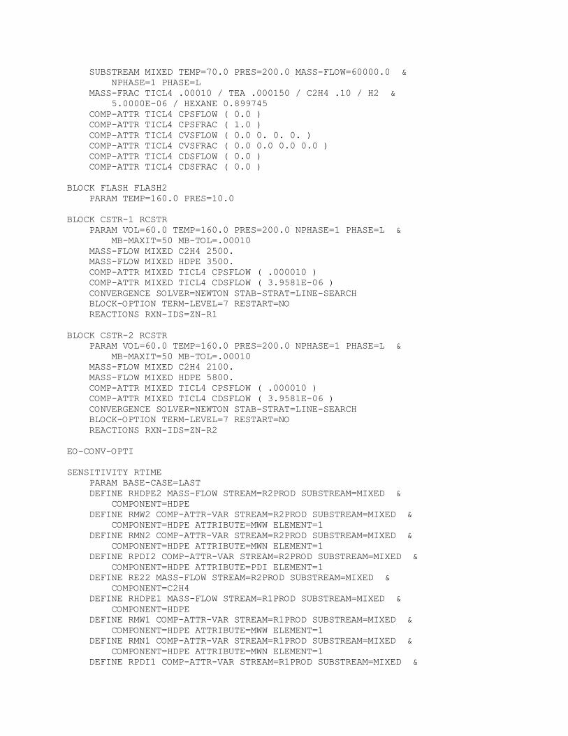
SUBSTREAM MIXED TEMP=70.0 PRES=200.0 MASS-FLOW=60000.0 & NPHASE=1 PHASE=L MASS-FRAC TICL4 .00010 / TEA .000150 / C2H4 .10 / H2 & 5.0000E-06 / HEXANE 0.899745 COMP-ATTR TICL4 CPSFLOW ( 0.0 ) COMP-ATTR TICL4 CPSFRAC ( 1.0 ) COMP-ATTR TICL4 CVSFLOW ( 0.0 0. 0. 0. ) COMP-ATTR TICL4 CVSFRAC ( 0.0 0.0 0.0 0.0 ) COMP-ATTR TICL4 CDSFLOW ( 0.0 ) COMP-ATTR TICL4 CDSFRAC ( 0.0 ) BLOCK FLASH FLASH2 PARAM TEMP=160.0 PRES=10.0 BLOCK CSTR-1 RCSTR PARAM VOL=60.0 TEMP=160.0 PRES=200.0 NPHASE=1 PHASE=L & MB-MAXIT=50 MB-TOL=.00010 MASS-FLOW MIXED C2H4 2500. MASS-FLOW MIXED HDPE 3500. COMP-ATTR MIXED TICL4 CPSFLOW ( .000010 ) COMP-ATTR MIXED TICL4 CDSFLOW ( 3.9581E-06 ) CONVERGENCE SOLVER=NEWTON STAB-STRAT=LINE-SEARCH BLOCK-OPTION TERM-LEVEL=7 RESTART=NO REACTIONS RXN-IDS=ZN-R1 BLOCK CSTR-2 RCSTR PARAM VOL=60.0 TEMP=160.0 PRES=200.0 NPHASE=1 PHASE=L & MB-MAXIT=50 MB-TOL=.00010 MASS-FLOW MIXED C2H4 2100. MASS-FLOW MIXED HDPE 5800. COMP-ATTR MIXED TICL4 CPSFLOW ( .000010 ) COMP-ATTR MIXED TICL4 CDSFLOW ( 3.9581E-06 ) CONVERGENCE SOLVER=NEWTON STAB-STRAT=LINE-SEARCH BLOCK-OPTION TERM-LEVEL=7 RESTART=NO REACTIONS RXN-IDS=ZN-R2 EO-CONV-OPTI SENSITIVITY RTIME PARAM BASE-CASE=LAST DEFINE RHDPE2 MASS-FLOW STREAM=R2PROD SUBSTREAM=MIXED & COMPONENT=HDPE DEFINE RMW2 COMP-ATTR-VAR STREAM=R2PROD SUBSTREAM=MIXED & COMPONENT=HDPE ATTRIBUTE=MWW ELEMENT=1 DEFINE RMN2 COMP-ATTR-VAR STREAM=R2PROD SUBSTREAM=MIXED & COMPONENT=HDPE ATTRIBUTE=MWN ELEMENT=1 DEFINE RPDI2 COMP-ATTR-VAR STREAM=R2PROD SUBSTREAM=MIXED & COMPONENT=HDPE ATTRIBUTE=PDI ELEMENT=1 DEFINE RE22 MASS-FLOW STREAM=R2PROD SUBSTREAM=MIXED & COMPONENT=C2H4 DEFINE RHDPE1 MASS-FLOW STREAM=R1PROD SUBSTREAM=MIXED & COMPONENT=HDPE DEFINE RMW1 COMP-ATTR-VAR STREAM=R1PROD SUBSTREAM=MIXED & COMPONENT=HDPE ATTRIBUTE=MWW ELEMENT=1 DEFINE RMN1 COMP-ATTR-VAR STREAM=R1PROD SUBSTREAM=MIXED & COMPONENT=HDPE ATTRIBUTE=MWN ELEMENT=1 DEFINE RPDI1 COMP-ATTR-VAR STREAM=R1PROD SUBSTREAM=MIXED &
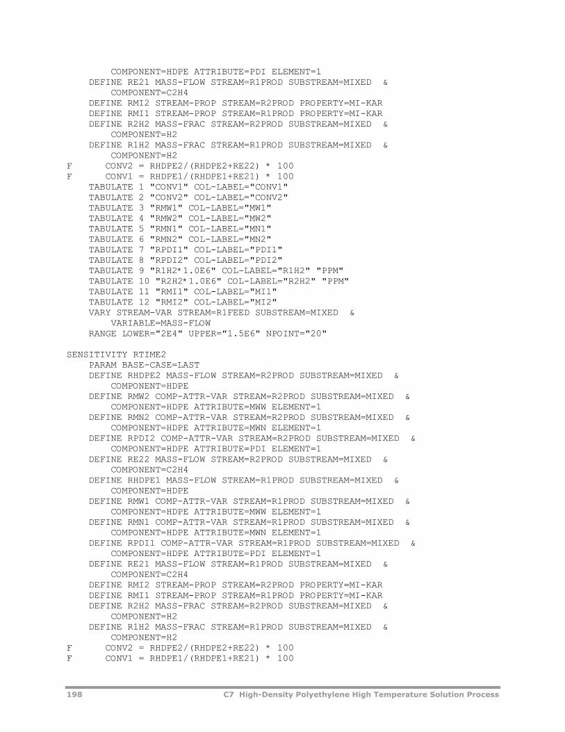
198 C7 High-Density Polyethylene High Temperature Solution Process
COMPONENT=HDPE ATTRIBUTE=PDI ELEMENT=1 DEFINE RE21 MASS-FLOW STREAM=R1PROD SUBSTREAM=MIXED & COMPONENT=C2H4 DEFINE RMI2 STREAM-PROP STREAM=R2PROD PROPERTY=MI-KAR DEFINE RMI1 STREAM-PROP STREAM=R1PROD PROPERTY=MI-KAR DEFINE R2H2 MASS-FRAC STREAM=R2PROD SUBSTREAM=MIXED & COMPONENT=H2 DEFINE R1H2 MASS-FRAC STREAM=R1PROD SUBSTREAM=MIXED & COMPONENT=H2 F CONV2 = RHDPE2/(RHDPE2+RE22) * 100 F CONV1 = RHDPE1/(RHDPE1+RE21) * 100 TABULATE 1 "CONV1" COL-LABEL="CONV1" TABULATE 2 "CONV2" COL-LABEL="CONV2" TABULATE 3 "RMW1" COL-LABEL="MW1" TABULATE 4 "RMW2" COL-LABEL="MW2" TABULATE 5 "RMN1" COL-LABEL="MN1" TABULATE 6 "RMN2" COL-LABEL="MN2" TABULATE 7 "RPDI1" COL-LABEL="PDI1" TABULATE 8 "RPDI2" COL-LABEL="PDI2" TABULATE 9 "R1H2*1.0E6" COL-LABEL="R1H2" "PPM" TABULATE 10 "R2H2*1.0E6" COL-LABEL="R2H2" "PPM" TABULATE 11 "RMI1" COL-LABEL="MI1" TABULATE 12 "RMI2" COL-LABEL="MI2" VARY STREAM-VAR STREAM=R1FEED SUBSTREAM=MIXED & VARIABLE=MASS-FLOW RANGE LOWER="2E4" UPPER="1.5E6" NPOINT="20" SENSITIVITY RTIME2 PARAM BASE-CASE=LAST DEFINE RHDPE2 MASS-FLOW STREAM=R2PROD SUBSTREAM=MIXED & COMPONENT=HDPE DEFINE RMW2 COMP-ATTR-VAR STREAM=R2PROD SUBSTREAM=MIXED & COMPONENT=HDPE ATTRIBUTE=MWW ELEMENT=1 DEFINE RMN2 COMP-ATTR-VAR STREAM=R2PROD SUBSTREAM=MIXED & COMPONENT=HDPE ATTRIBUTE=MWN ELEMENT=1 DEFINE RPDI2 COMP-ATTR-VAR STREAM=R2PROD SUBSTREAM=MIXED & COMPONENT=HDPE ATTRIBUTE=PDI ELEMENT=1 DEFINE RE22 MASS-FLOW STREAM=R2PROD SUBSTREAM=MIXED & COMPONENT=C2H4 DEFINE RHDPE1 MASS-FLOW STREAM=R1PROD SUBSTREAM=MIXED & COMPONENT=HDPE DEFINE RMW1 COMP-ATTR-VAR STREAM=R1PROD SUBSTREAM=MIXED & COMPONENT=HDPE ATTRIBUTE=MWW ELEMENT=1 DEFINE RMN1 COMP-ATTR-VAR STREAM=R1PROD SUBSTREAM=MIXED & COMPONENT=HDPE ATTRIBUTE=MWN ELEMENT=1 DEFINE RPDI1 COMP-ATTR-VAR STREAM=R1PROD SUBSTREAM=MIXED & COMPONENT=HDPE ATTRIBUTE=PDI ELEMENT=1 DEFINE RE21 MASS-FLOW STREAM=R1PROD SUBSTREAM=MIXED & COMPONENT=C2H4 DEFINE RMI2 STREAM-PROP STREAM=R2PROD PROPERTY=MI-KAR DEFINE RMI1 STREAM-PROP STREAM=R1PROD PROPERTY=MI-KAR DEFINE R2H2 MASS-FRAC STREAM=R2PROD SUBSTREAM=MIXED & COMPONENT=H2 DEFINE R1H2 MASS-FRAC STREAM=R1PROD SUBSTREAM=MIXED & COMPONENT=H2 F CONV2 = RHDPE2/(RHDPE2+RE22) * 100 F CONV1 = RHDPE1/(RHDPE1+RE21) * 100
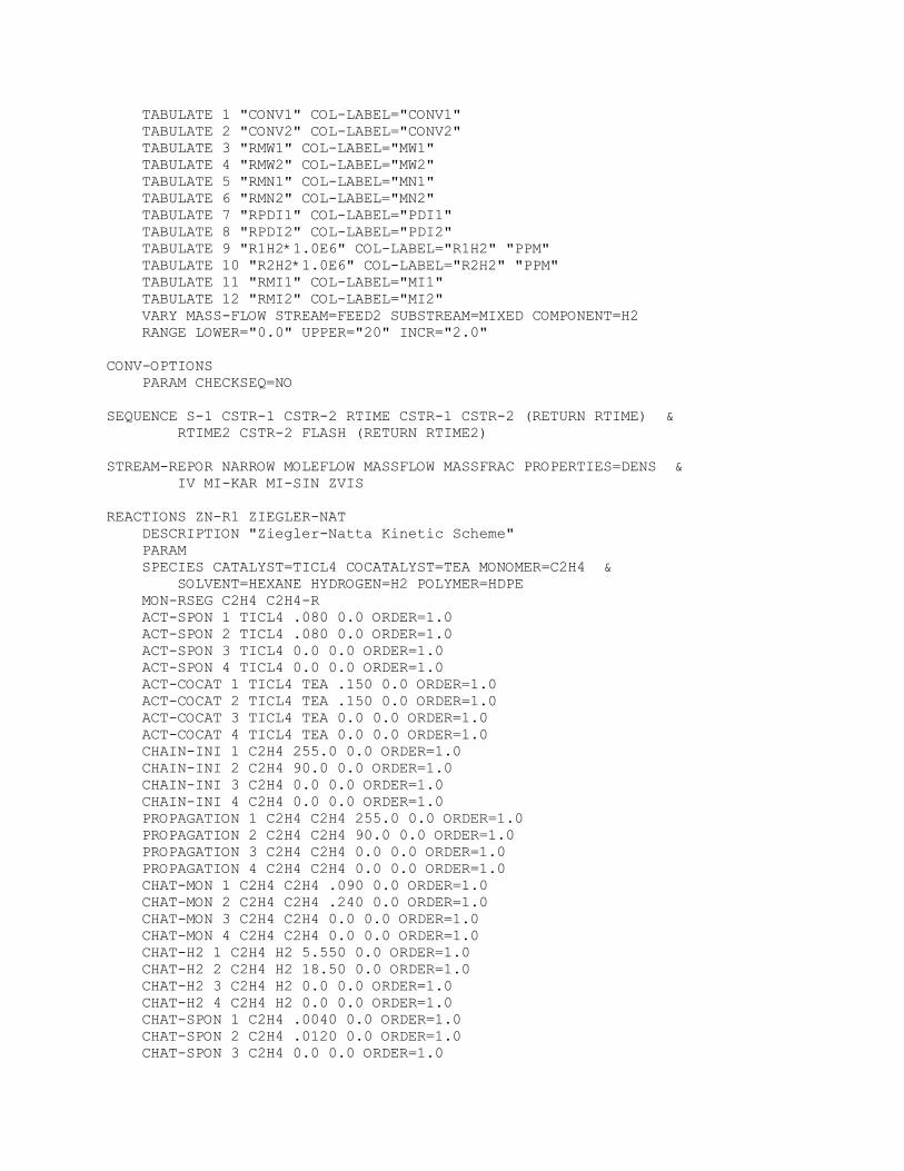
TABULATE 1 "CONV1" COL-LABEL="CONV1" TABULATE 2 "CONV2" COL-LABEL="CONV2" TABULATE 3 "RMW1" COL-LABEL="MW1" TABULATE 4 "RMW2" COL-LABEL="MW2" TABULATE 5 "RMN1" COL-LABEL="MN1" TABULATE 6 "RMN2" COL-LABEL="MN2" TABULATE 7 "RPDI1" COL-LABEL="PDI1" TABULATE 8 "RPDI2" COL-LABEL="PDI2" TABULATE 9 "R1H2*1.0E6" COL-LABEL="R1H2" "PPM" TABULATE 10 "R2H2*1.0E6" COL-LABEL="R2H2" "PPM" TABULATE 11 "RMI1" COL-LABEL="MI1" TABULATE 12 "RMI2" COL-LABEL="MI2" VARY MASS-FLOW STREAM=FEED2 SUBSTREAM=MIXED COMPONENT=H2 RANGE LOWER="0.0" UPPER="20" INCR="2.0" CONV-OPTIONS PARAM CHECKSEQ=NO SEQUENCE S-1 CSTR-1 CSTR-2 RTIME CSTR-1 CSTR-2 (RETURN RTIME) & RTIME2 CSTR-2 FLASH (RETURN RTIME2) STREAM-REPOR NARROW MOLEFLOW MASSFLOW MASSFRAC PROPERTIES=DENS & IV MI-KAR MI-SIN ZVIS REACTIONS ZN-R1 ZIEGLER-NAT DESCRIPTION "Ziegler-Natta Kinetic Scheme" PARAM SPECIES CATALYST=TICL4 COCATALYST=TEA MONOMER=C2H4 & SOLVENT=HEXANE HYDROGEN=H2 POLYMER=HDPE MON-RSEG C2H4 C2H4-R ACT-SPON 1 TICL4 .080 0.0 ORDER=1.0 ACT-SPON 2 TICL4 .080 0.0 ORDER=1.0 ACT-SPON 3 TICL4 0.0 0.0 ORDER=1.0 ACT-SPON 4 TICL4 0.0 0.0 ORDER=1.0 ACT-COCAT 1 TICL4 TEA .150 0.0 ORDER=1.0 ACT-COCAT 2 TICL4 TEA .150 0.0 ORDER=1.0 ACT-COCAT 3 TICL4 TEA 0.0 0.0 ORDER=1.0 ACT-COCAT 4 TICL4 TEA 0.0 0.0 ORDER=1.0 CHAIN-INI 1 C2H4 255.0 0.0 ORDER=1.0 CHAIN-INI 2 C2H4 90.0 0.0 ORDER=1.0 CHAIN-INI 3 C2H4 0.0 0.0 ORDER=1.0 CHAIN-INI 4 C2H4 0.0 0.0 ORDER=1.0 PROPAGATION 1 C2H4 C2H4 255.0 0.0 ORDER=1.0 PROPAGATION 2 C2H4 C2H4 90.0 0.0 ORDER=1.0 PROPAGATION 3 C2H4 C2H4 0.0 0.0 ORDER=1.0 PROPAGATION 4 C2H4 C2H4 0.0 0.0 ORDER=1.0 CHAT-MON 1 C2H4 C2H4 .090 0.0 ORDER=1.0 CHAT-MON 2 C2H4 C2H4 .240 0.0 ORDER=1.0 CHAT-MON 3 C2H4 C2H4 0.0 0.0 ORDER=1.0 CHAT-MON 4 C2H4 C2H4 0.0 0.0 ORDER=1.0 CHAT-H2 1 C2H4 H2 5.550 0.0 ORDER=1.0 CHAT-H2 2 C2H4 H2 18.50 0.0 ORDER=1.0 CHAT-H2 3 C2H4 H2 0.0 0.0 ORDER=1.0 CHAT-H2 4 C2H4 H2 0.0 0.0 ORDER=1.0 CHAT-SPON 1 C2H4 .0040 0.0 ORDER=1.0 CHAT-SPON 2 C2H4 .0120 0.0 ORDER=1.0 CHAT-SPON 3 C2H4 0.0 0.0 ORDER=1.0
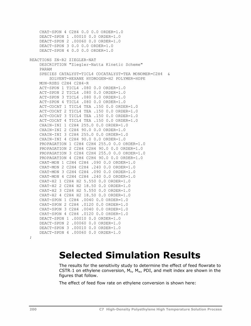
200 C7 High-Density Polyethylene High Temperature Solution Process
CHAT-SPON 4 C2H4 0.0 0.0 ORDER=1.0 DEACT-SPON 1 .00010 0.0 ORDER=1.0 DEACT-SPON 2 .00060 0.0 ORDER=1.0 DEACT-SPON 3 0.0 0.0 ORDER=1.0 DEACT-SPON 4 0.0 0.0 ORDER=1.0 REACTIONS ZN-R2 ZIEGLER-NAT DESCRIPTION "Ziegler-Natta Kinetic Scheme" PARAM SPECIES CATALYST=TICL4 COCATALYST=TEA MONOMER=C2H4 & SOLVENT=HEXANE HYDROGEN=H2 POLYMER=HDPE MON-RSEG C2H4 C2H4-R ACT-SPON 1 TICL4 .080 0.0 ORDER=1.0 ACT-SPON 2 TICL4 .080 0.0 ORDER=1.0 ACT-SPON 3 TICL4 .080 0.0 ORDER=1.0 ACT-SPON 4 TICL4 .080 0.0 ORDER=1.0 ACT-COCAT 1 TICL4 TEA .150 0.0 ORDER=1.0 ACT-COCAT 2 TICL4 TEA .150 0.0 ORDER=1.0 ACT-COCAT 3 TICL4 TEA .150 0.0 ORDER=1.0 ACT-COCAT 4 TICL4 TEA .150 0.0 ORDER=1.0 CHAIN-INI 1 C2H4 255.0 0.0 ORDER=1.0 CHAIN-INI 2 C2H4 90.0 0.0 ORDER=1.0 CHAIN-INI 3 C2H4 255.0 0.0 ORDER=1.0 CHAIN-INI 4 C2H4 90.0 0.0 ORDER=1.0 PROPAGATION 1 C2H4 C2H4 255.0 0.0 ORDER=1.0 PROPAGATION 2 C2H4 C2H4 90.0 0.0 ORDER=1.0 PROPAGATION 3 C2H4 C2H4 255.0 0.0 ORDER=1.0 PROPAGATION 4 C2H4 C2H4 90.0 0.0 ORDER=1.0 CHAT-MON 1 C2H4 C2H4 .090 0.0 ORDER=1.0 CHAT-MON 2 C2H4 C2H4 .240 0.0 ORDER=1.0 CHAT-MON 3 C2H4 C2H4 .090 0.0 ORDER=1.0 CHAT-MON 4 C2H4 C2H4 .240 0.0 ORDER=1.0 CHAT-H2 1 C2H4 H2 5.550 0.0 ORDER=1.0 CHAT-H2 2 C2H4 H2 18.50 0.0 ORDER=1.0 CHAT-H2 3 C2H4 H2 5.550 0.0 ORDER=1.0 CHAT-H2 4 C2H4 H2 18.50 0.0 ORDER=1.0 CHAT-SPON 1 C2H4 .0040 0.0 ORDER=1.0 CHAT-SPON 2 C2H4 .0120 0.0 ORDER=1.0 CHAT-SPON 3 C2H4 .0040 0.0 ORDER=1.0 CHAT-SPON 4 C2H4 .0120 0.0 ORDER=1.0 DEACT-SPON 1 .00010 0.0 ORDER=1.0 DEACT-SPON 2 .00060 0.0 ORDER=1.0 DEACT-SPON 3 .00010 0.0 ORDER=1.0 DEACT-SPON 4 .00060 0.0 ORDER=1.0 ;
Selected Simulation Results The results for the sensitivity study to determine the effect of feed flowrate to CSTR-1 on ethylene conversion, Mn, Mw, PDI, and melt index are shown in the figures that follow.
The effect of feed flow rate on ethylene conversion is shown here:
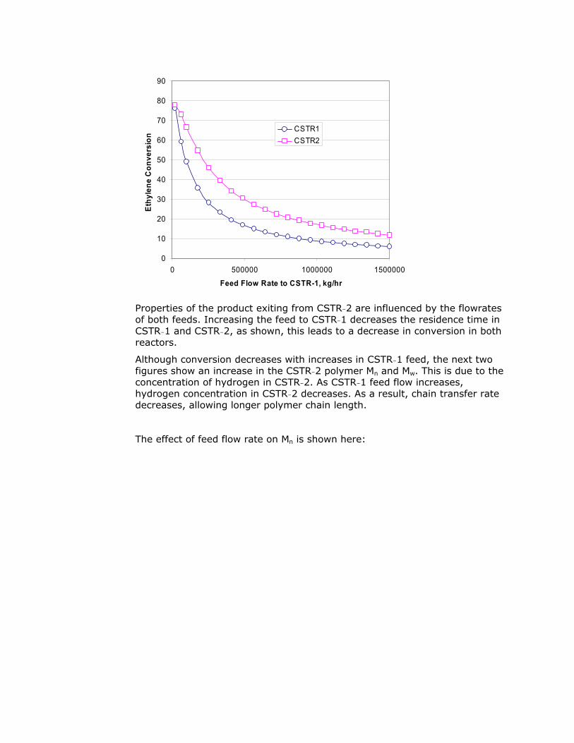
0
10
20
30
40
50
60
70
80
90
0 500000 1000000 1500000
Feed Flow Rate to CSTR-1, kg/hr
Ethy
lene
Con
vers
ion
CSTR1CSTR2
Properties of the product exiting from CSTR-2 are influenced by the flowrates of both feeds. Increasing the feed to CSTR-1 decreases the residence time in CSTR-1 and CSTR-2, as shown, this leads to a decrease in conversion in both reactors.
Although conversion decreases with increases in CSTR-1 feed, the next two figures show an increase in the CSTR-2 polymer Mn and Mw. This is due to the concentration of hydrogen in CSTR-2. As CSTR-1 feed flow increases, hydrogen concentration in CSTR-2 decreases. As a result, chain transfer rate decreases, allowing longer polymer chain length.
The effect of feed flow rate on Mn is shown here:
202 C7 High-Density Polyethylene High Temperature Solution Process
20000
25000
30000
35000
40000
0 500000 1000000 1500000
Feed Flow Rate to CSTR-1, kg/hr
Mn
CSTR1CSTR2
The effect of feed flow rate on Mw is shown here:
80000
85000
90000
95000
100000
105000
110000
115000
120000
0 500000 1000000 1500000
Feed Flow Rate to CSTR-1, kg/hr
Mw
CSTR1CSTR2
The effect of feed flow rate on the hydrogen concentration (PPM) is shown here:
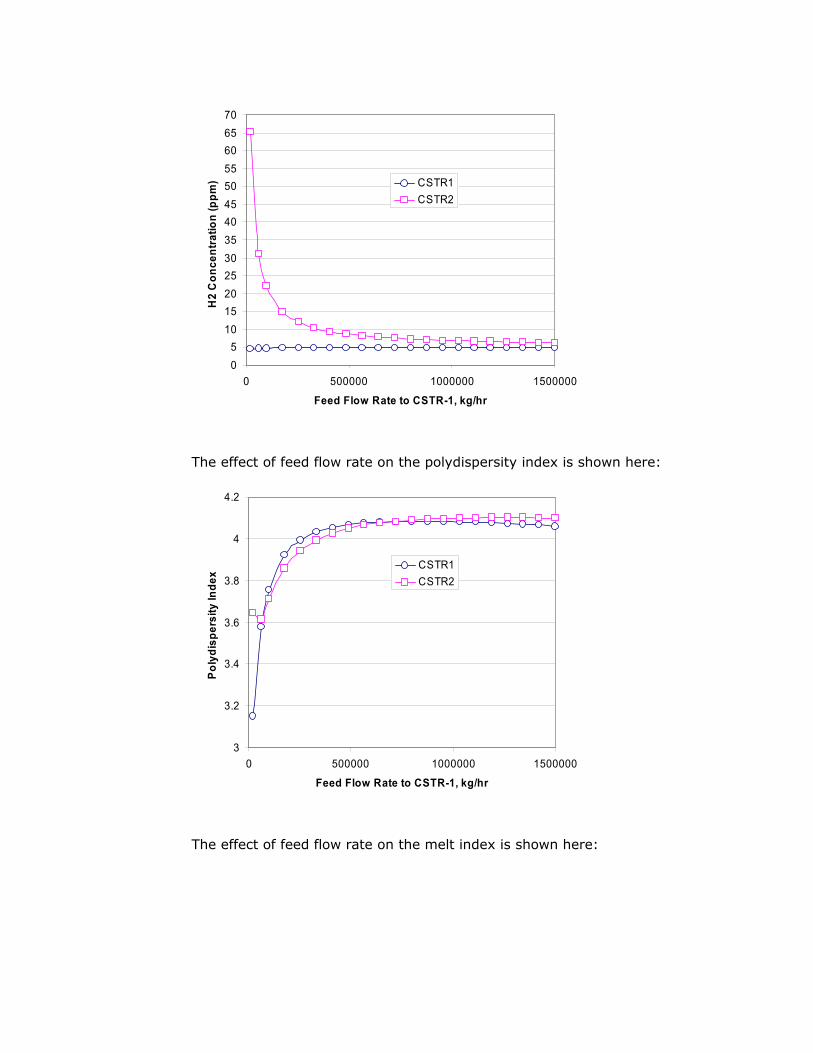
05
10152025303540455055606570
0 500000 1000000 1500000
Feed Flow Rate to CSTR-1, kg/hr
H2
Con
cent
ratio
n (p
pm) CSTR1
CSTR2
The effect of feed flow rate on the polydispersity index is shown here:
3
3.2
3.4
3.6
3.8
4
4.2
0 500000 1000000 1500000
Feed Flow Rate to CSTR-1, kg/hr
Poly
disp
ersi
ty In
dex
CSTR1CSTR2
The effect of feed flow rate on the melt index is shown here:
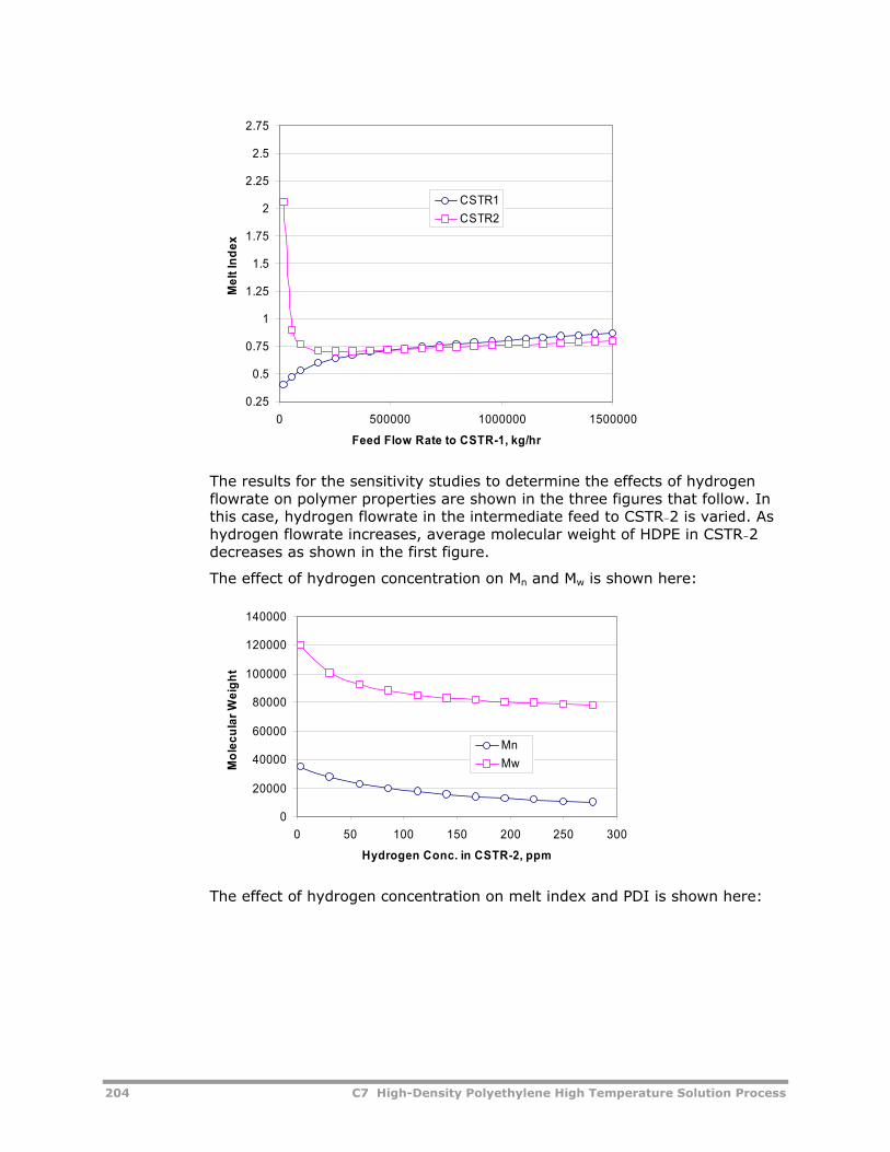
204 C7 High-Density Polyethylene High Temperature Solution Process
0.25
0.5
0.75
1
1.25
1.5
1.75
2
2.25
2.5
2.75
0 500000 1000000 1500000
Feed Flow Rate to CSTR-1, kg/hr
Mel
t Ind
ex
CSTR1CSTR2
The results for the sensitivity studies to determine the effects of hydrogen flowrate on polymer properties are shown in the three figures that follow. In this case, hydrogen flowrate in the intermediate feed to CSTR-2 is varied. As hydrogen flowrate increases, average molecular weight of HDPE in CSTR-2 decreases as shown in the first figure.
The effect of hydrogen concentration on Mn and Mw is shown here:
0
20000
40000
60000
80000
100000
120000
140000
0 50 100 150 200 250 300
Hydrogen Conc. in CSTR-2, ppm
Mol
ecul
ar W
eigh
t
Mn Mw
The effect of hydrogen concentration on melt index and PDI is shown here:
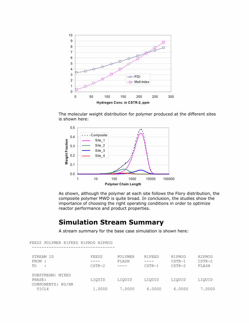
01
2345
678
910
0 50 100 150 200 250 300
Hydrogen Conc. in CSTR-2, ppm
PDIMelt Index
The molecular weight distribution for polymer produced at the different sites is shown here:
0.0
0.1
0.2
0.3
0.4
0.5
1 10 100 1000 10000 100000Polymer Chain Length
Wei
ght F
ract
ion
Composite Site_1 Site_2 Site_3 Site_4
As shown, although the polymer at each site follows the Flory distribution, the composite polymer MWD is quite broad. In conclusion, the studies show the importance of choosing the right operating conditions in order to optimize reactor performance and product properties.
Simulation Stream Summary A stream summary for the base case simulation is shown here:
FEED2 POLYMER R1FEED R1PROD R2PROD ---------------------------------- STREAM ID FEED2 POLYMER R1FEED R1PROD R2PROD FROM : ---- FLASH ---- CSTR-1 CSTR-2 TO : CSTR-2 ---- CSTR-1 CSTR-2 FLASH SUBSTREAM: MIXED PHASE: LIQUID LIQUID LIQUID LIQUID LIQUID COMPONENTS: KG/HR TICL4 1.0000 7.0000 6.0000 6.0000 7.0000
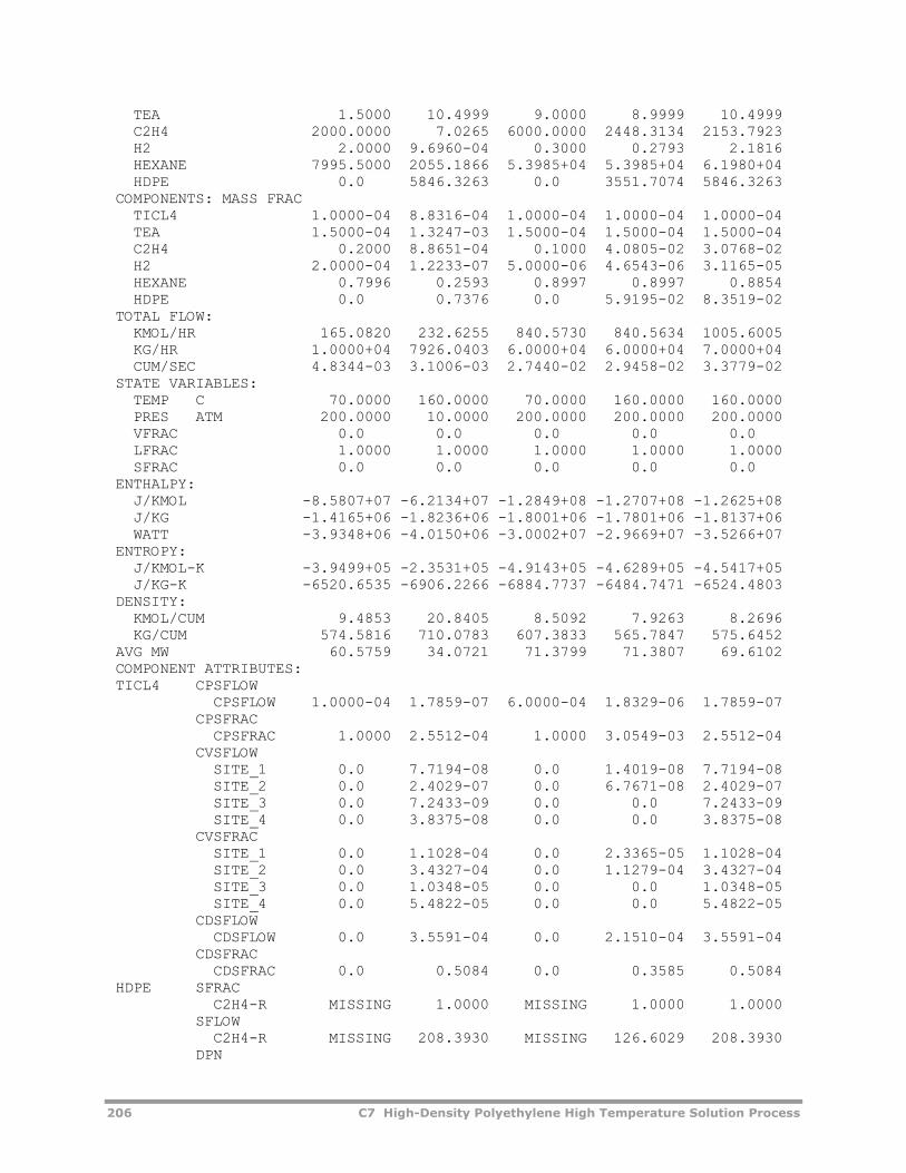
206 C7 High-Density Polyethylene High Temperature Solution Process
TEA 1.5000 10.4999 9.0000 8.9999 10.4999 C2H4 2000.0000 7.0265 6000.0000 2448.3134 2153.7923 H2 2.0000 9.6960-04 0.3000 0.2793 2.1816 HEXANE 7995.5000 2055.1866 5.3985+04 5.3985+04 6.1980+04 HDPE 0.0 5846.3263 0.0 3551.7074 5846.3263 COMPONENTS: MASS FRAC TICL4 1.0000-04 8.8316-04 1.0000-04 1.0000-04 1.0000-04 TEA 1.5000-04 1.3247-03 1.5000-04 1.5000-04 1.5000-04 C2H4 0.2000 8.8651-04 0.1000 4.0805-02 3.0768-02 H2 2.0000-04 1.2233-07 5.0000-06 4.6543-06 3.1165-05 HEXANE 0.7996 0.2593 0.8997 0.8997 0.8854 HDPE 0.0 0.7376 0.0 5.9195-02 8.3519-02 TOTAL FLOW: KMOL/HR 165.0820 232.6255 840.5730 840.5634 1005.6005 KG/HR 1.0000+04 7926.0403 6.0000+04 6.0000+04 7.0000+04 CUM/SEC 4.8344-03 3.1006-03 2.7440-02 2.9458-02 3.3779-02 STATE VARIABLES: TEMP C 70.0000 160.0000 70.0000 160.0000 160.0000 PRES ATM 200.0000 10.0000 200.0000 200.0000 200.0000 VFRAC 0.0 0.0 0.0 0.0 0.0 LFRAC 1.0000 1.0000 1.0000 1.0000 1.0000 SFRAC 0.0 0.0 0.0 0.0 0.0 ENTHALPY: J/KMOL -8.5807+07 -6.2134+07 -1.2849+08 -1.2707+08 -1.2625+08 J/KG -1.4165+06 -1.8236+06 -1.8001+06 -1.7801+06 -1.8137+06 WATT -3.9348+06 -4.0150+06 -3.0002+07 -2.9669+07 -3.5266+07 ENTROPY: J/KMOL-K -3.9499+05 -2.3531+05 -4.9143+05 -4.6289+05 -4.5417+05 J/KG-K -6520.6535 -6906.2266 -6884.7737 -6484.7471 -6524.4803 DENSITY: KMOL/CUM 9.4853 20.8405 8.5092 7.9263 8.2696 KG/CUM 574.5816 710.0783 607.3833 565.7847 575.6452 AVG MW 60.5759 34.0721 71.3799 71.3807 69.6102 COMPONENT ATTRIBUTES: TICL4 CPSFLOW CPSFLOW 1.0000-04 1.7859-07 6.0000-04 1.8329-06 1.7859-07 CPSFRAC CPSFRAC 1.0000 2.5512-04 1.0000 3.0549-03 2.5512-04 CVSFLOW SITE_1 0.0 7.7194-08 0.0 1.4019-08 7.7194-08 SITE_2 0.0 2.4029-07 0.0 6.7671-08 2.4029-07 SITE_3 0.0 7.2433-09 0.0 0.0 7.2433-09 SITE_4 0.0 3.8375-08 0.0 0.0 3.8375-08 CVSFRAC SITE_1 0.0 1.1028-04 0.0 2.3365-05 1.1028-04 SITE_2 0.0 3.4327-04 0.0 1.1279-04 3.4327-04 SITE_3 0.0 1.0348-05 0.0 0.0 1.0348-05 SITE_4 0.0 5.4822-05 0.0 0.0 5.4822-05 CDSFLOW CDSFLOW 0.0 3.5591-04 0.0 2.1510-04 3.5591-04 CDSFRAC CDSFRAC 0.0 0.5084 0.0 0.3585 0.5084 HDPE SFRAC C2H4-R MISSING 1.0000 MISSING 1.0000 1.0000 SFLOW C2H4-R MISSING 208.3930 MISSING 126.6029 208.3930 DPN
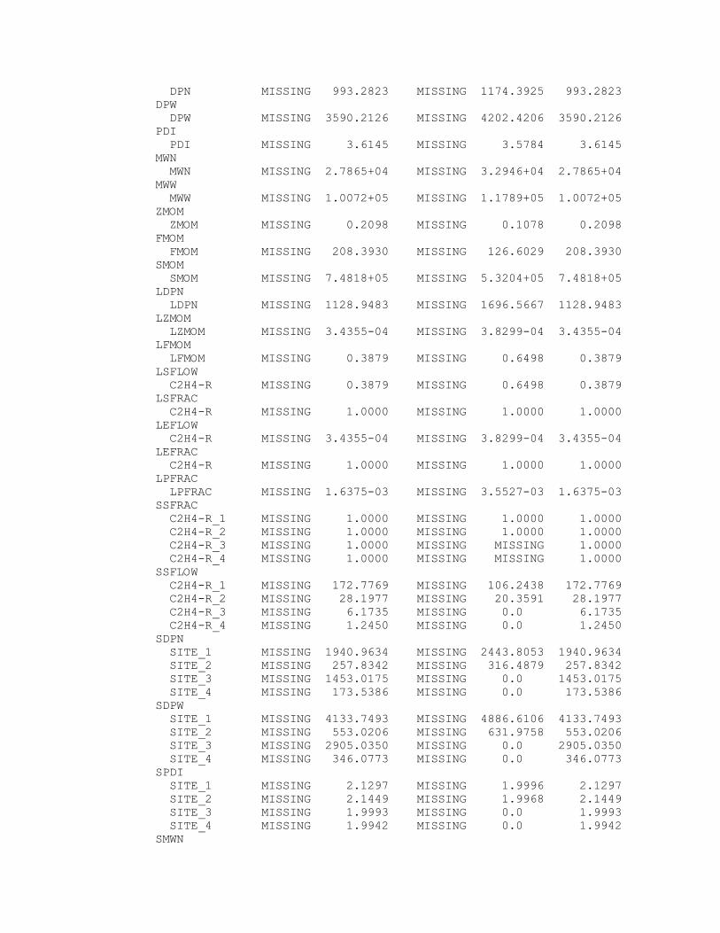
DPN MISSING 993.2823 MISSING 1174.3925 993.2823 DPW DPW MISSING 3590.2126 MISSING 4202.4206 3590.2126 PDI PDI MISSING 3.6145 MISSING 3.5784 3.6145 MWN MWN MISSING 2.7865+04 MISSING 3.2946+04 2.7865+04 MWW MWW MISSING 1.0072+05 MISSING 1.1789+05 1.0072+05 ZMOM ZMOM MISSING 0.2098 MISSING 0.1078 0.2098 FMOM FMOM MISSING 208.3930 MISSING 126.6029 208.3930 SMOM SMOM MISSING 7.4818+05 MISSING 5.3204+05 7.4818+05 LDPN LDPN MISSING 1128.9483 MISSING 1696.5667 1128.9483 LZMOM LZMOM MISSING 3.4355-04 MISSING 3.8299-04 3.4355-04 LFMOM LFMOM MISSING 0.3879 MISSING 0.6498 0.3879 LSFLOW C2H4-R MISSING 0.3879 MISSING 0.6498 0.3879 LSFRAC C2H4-R MISSING 1.0000 MISSING 1.0000 1.0000 LEFLOW C2H4-R MISSING 3.4355-04 MISSING 3.8299-04 3.4355-04 LEFRAC C2H4-R MISSING 1.0000 MISSING 1.0000 1.0000 LPFRAC LPFRAC MISSING 1.6375-03 MISSING 3.5527-03 1.6375-03 SSFRAC C2H4-R_1 MISSING 1.0000 MISSING 1.0000 1.0000 C2H4-R_2 MISSING 1.0000 MISSING 1.0000 1.0000 C2H4-R_3 MISSING 1.0000 MISSING MISSING 1.0000 C2H4-R_4 MISSING 1.0000 MISSING MISSING 1.0000 SSFLOW C2H4-R_1 MISSING 172.7769 MISSING 106.2438 172.7769 C2H4-R_2 MISSING 28.1977 MISSING 20.3591 28.1977 C2H4-R_3 MISSING 6.1735 MISSING 0.0 6.1735 C2H4-R_4 MISSING 1.2450 MISSING 0.0 1.2450 SDPN SITE_1 MISSING 1940.9634 MISSING 2443.8053 1940.9634 SITE_2 MISSING 257.8342 MISSING 316.4879 257.8342 SITE_3 MISSING 1453.0175 MISSING 0.0 1453.0175 SITE_4 MISSING 173.5386 MISSING 0.0 173.5386 SDPW SITE_1 MISSING 4133.7493 MISSING 4886.6106 4133.7493 SITE_2 MISSING 553.0206 MISSING 631.9758 553.0206 SITE_3 MISSING 2905.0350 MISSING 0.0 2905.0350 SITE_4 MISSING 346.0773 MISSING 0.0 346.0773 SPDI SITE_1 MISSING 2.1297 MISSING 1.9996 2.1297 SITE_2 MISSING 2.1449 MISSING 1.9968 2.1449 SITE_3 MISSING 1.9993 MISSING 0.0 1.9993 SITE_4 MISSING 1.9942 MISSING 0.0 1.9942 SMWN
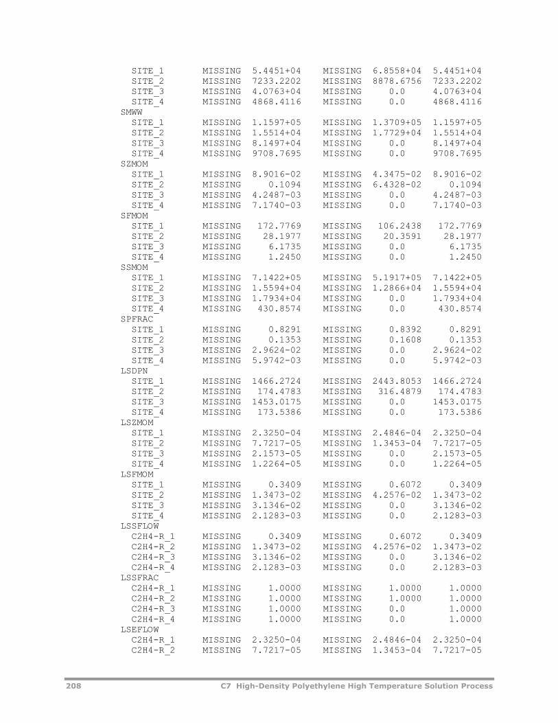
208 C7 High-Density Polyethylene High Temperature Solution Process
SITE_1 MISSING 5.4451+04 MISSING 6.8558+04 5.4451+04 SITE_2 MISSING 7233.2202 MISSING 8878.6756 7233.2202 SITE_3 MISSING 4.0763+04 MISSING 0.0 4.0763+04 SITE_4 MISSING 4868.4116 MISSING 0.0 4868.4116 SMWW SITE_1 MISSING 1.1597+05 MISSING 1.3709+05 1.1597+05 SITE_2 MISSING 1.5514+04 MISSING 1.7729+04 1.5514+04 SITE_3 MISSING 8.1497+04 MISSING 0.0 8.1497+04 SITE_4 MISSING 9708.7695 MISSING 0.0 9708.7695 SZMOM SITE_1 MISSING 8.9016-02 MISSING 4.3475-02 8.9016-02 SITE_2 MISSING 0.1094 MISSING 6.4328-02 0.1094 SITE_3 MISSING 4.2487-03 MISSING 0.0 4.2487-03 SITE_4 MISSING 7.1740-03 MISSING 0.0 7.1740-03 SFMOM SITE_1 MISSING 172.7769 MISSING 106.2438 172.7769 SITE_2 MISSING 28.1977 MISSING 20.3591 28.1977 SITE_3 MISSING 6.1735 MISSING 0.0 6.1735 SITE_4 MISSING 1.2450 MISSING 0.0 1.2450 SSMOM SITE_1 MISSING 7.1422+05 MISSING 5.1917+05 7.1422+05 SITE_2 MISSING 1.5594+04 MISSING 1.2866+04 1.5594+04 SITE_3 MISSING 1.7934+04 MISSING 0.0 1.7934+04 SITE_4 MISSING 430.8574 MISSING 0.0 430.8574 SPFRAC SITE_1 MISSING 0.8291 MISSING 0.8392 0.8291 SITE_2 MISSING 0.1353 MISSING 0.1608 0.1353 SITE_3 MISSING 2.9624-02 MISSING 0.0 2.9624-02 SITE_4 MISSING 5.9742-03 MISSING 0.0 5.9742-03 LSDPN SITE_1 MISSING 1466.2724 MISSING 2443.8053 1466.2724 SITE_2 MISSING 174.4783 MISSING 316.4879 174.4783 SITE_3 MISSING 1453.0175 MISSING 0.0 1453.0175 SITE_4 MISSING 173.5386 MISSING 0.0 173.5386 LSZMOM SITE_1 MISSING 2.3250-04 MISSING 2.4846-04 2.3250-04 SITE_2 MISSING 7.7217-05 MISSING 1.3453-04 7.7217-05 SITE_3 MISSING 2.1573-05 MISSING 0.0 2.1573-05 SITE_4 MISSING 1.2264-05 MISSING 0.0 1.2264-05 LSFMOM SITE_1 MISSING 0.3409 MISSING 0.6072 0.3409 SITE_2 MISSING 1.3473-02 MISSING 4.2576-02 1.3473-02 SITE_3 MISSING 3.1346-02 MISSING 0.0 3.1346-02 SITE_4 MISSING 2.1283-03 MISSING 0.0 2.1283-03 LSSFLOW C2H4-R_1 MISSING 0.3409 MISSING 0.6072 0.3409 C2H4-R_2 MISSING 1.3473-02 MISSING 4.2576-02 1.3473-02 C2H4-R_3 MISSING 3.1346-02 MISSING 0.0 3.1346-02 C2H4-R_4 MISSING 2.1283-03 MISSING 0.0 2.1283-03 LSSFRAC C2H4-R_1 MISSING 1.0000 MISSING 1.0000 1.0000 C2H4-R_2 MISSING 1.0000 MISSING 1.0000 1.0000 C2H4-R_3 MISSING 1.0000 MISSING 0.0 1.0000 C2H4-R_4 MISSING 1.0000 MISSING 0.0 1.0000 LSEFLOW C2H4-R_1 MISSING 2.3250-04 MISSING 2.4846-04 2.3250-04 C2H4-R_2 MISSING 7.7217-05 MISSING 1.3453-04 7.7217-05
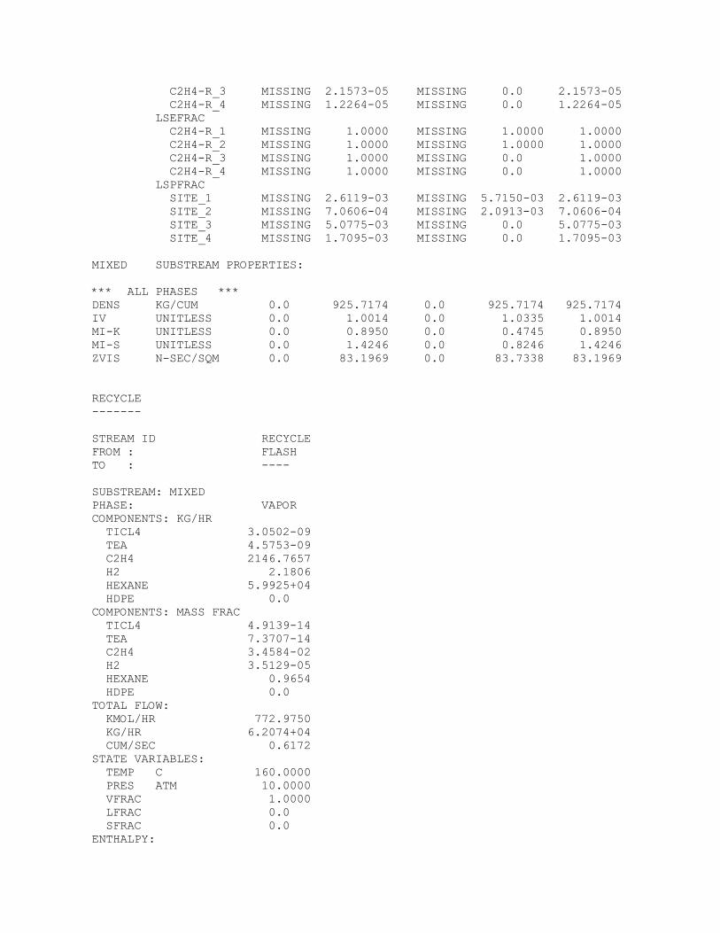
C2H4-R_3 MISSING 2.1573-05 MISSING 0.0 2.1573-05 C2H4-R_4 MISSING 1.2264-05 MISSING 0.0 1.2264-05 LSEFRAC C2H4-R_1 MISSING 1.0000 MISSING 1.0000 1.0000 C2H4-R_2 MISSING 1.0000 MISSING 1.0000 1.0000 C2H4-R_3 MISSING 1.0000 MISSING 0.0 1.0000 C2H4-R_4 MISSING 1.0000 MISSING 0.0 1.0000 LSPFRAC SITE_1 MISSING 2.6119-03 MISSING 5.7150-03 2.6119-03 SITE_2 MISSING 7.0606-04 MISSING 2.0913-03 7.0606-04 SITE_3 MISSING 5.0775-03 MISSING 0.0 5.0775-03 SITE_4 MISSING 1.7095-03 MISSING 0.0 1.7095-03 MIXED SUBSTREAM PROPERTIES: *** ALL PHASES *** DENS KG/CUM 0.0 925.7174 0.0 925.7174 925.7174 IV UNITLESS 0.0 1.0014 0.0 1.0335 1.0014 MI-K UNITLESS 0.0 0.8950 0.0 0.4745 0.8950 MI-S UNITLESS 0.0 1.4246 0.0 0.8246 1.4246 ZVIS N-SEC/SQM 0.0 83.1969 0.0 83.7338 83.1969 RECYCLE ------- STREAM ID RECYCLE FROM : FLASH TO : ---- SUBSTREAM: MIXED PHASE: VAPOR COMPONENTS: KG/HR TICL4 3.0502-09 TEA 4.5753-09 C2H4 2146.7657 H2 2.1806 HEXANE 5.9925+04 HDPE 0.0 COMPONENTS: MASS FRAC TICL4 4.9139-14 TEA 7.3707-14 C2H4 3.4584-02 H2 3.5129-05 HEXANE 0.9654 HDPE 0.0 TOTAL FLOW: KMOL/HR 772.9750 KG/HR 6.2074+04 CUM/SEC 0.6172 STATE VARIABLES: TEMP C 160.0000 PRES ATM 10.0000 VFRAC 1.0000 LFRAC 0.0 SFRAC 0.0 ENTHALPY:
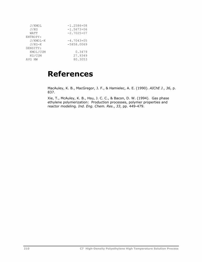
210 C7 High-Density Polyethylene High Temperature Solution Process
J/KMOL -1.2586+08 J/KG -1.5673+06 WATT -2.7025+07 ENTROPY: J/KMOL-K -4.7043+05 J/KG-K -5858.0069 DENSITY: KMOL/CUM 0.3479 KG/CUM 27.9349 AVG MW 80.3053
References
MacAuley, K. B., MacGregor, J. F., & Hamielec, A. E. (1990). AIChE J., 36, p. 837.
Xie, T., McAuley, K. B., Hsu, J. C. C., & Bacon, D. W. (1994). Gas phase ethylene polymerization: Production processes, polymer properties and reactor modeling. Ind. Eng. Chem. Res., 33, pp. 449-479.
C8 Low-Density Polyethylene High Pressure Process
The LDPE high-pressure process model illustrates the use of Aspen Polymers Plus to model a high pressure free-radical process for low-density polyethylene. The model considers the tubular jacketed reactor along with the post-polymerization devolatization. Among the parameters studied in the model are reactor temperature profile, monomer conversion, polymer molecular weight and degree of branching.
About This Process Low density polyethylene (LDPE), is part of the polyolefin family of polymers. This polymer exhibits a number of desirable properties, including strength, flexibility, impact resistance, resistance to solvents, to chemicals, and to oxidating agents. For this reason, it is one of the highest volume polymers in terms of production.
LDPE is produced by free-radical polymerization. It has been produced in batch processes. However, continuous processes are more commonly found, because they allow better control of the polymerization. Polymerization is carried out in tubular and autoclave reactors under high pressure (1300-3400 atm), and high temperatures (150-340°C). At such high compression states, the gaseous ethylene monomer behaves like a liquid. The reactor of choice for the production of LDPE is a tubular reactor. Some processes involve multizone tubular reactors with multiple initiator injection points along the length of the reactor.
Process Definition In this example, polymerization of ethylene is carried out in a jacketed tubular reactor divided into four sections, with two initiator injection points.
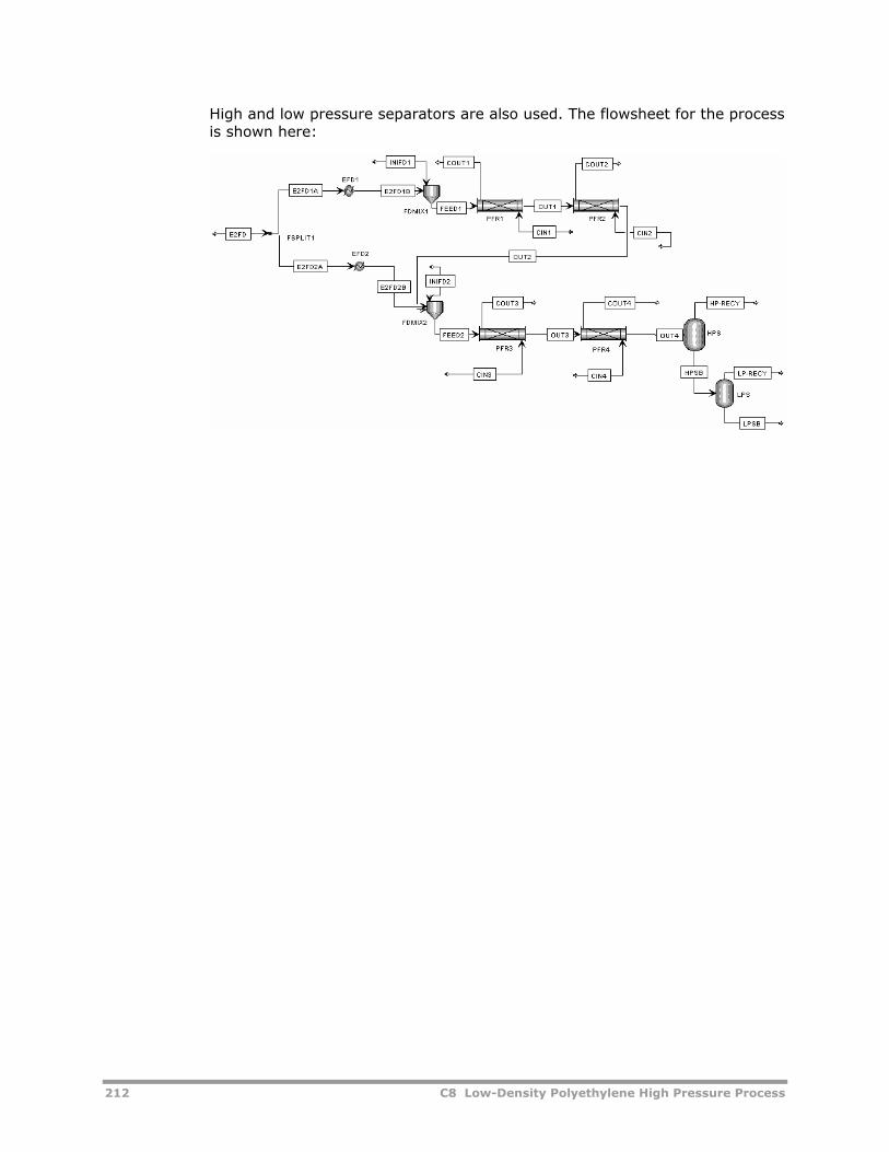
212 C8 Low-Density Polyethylene High Pressure Process
High and low pressure separators are also used. The flowsheet for the process is shown here:
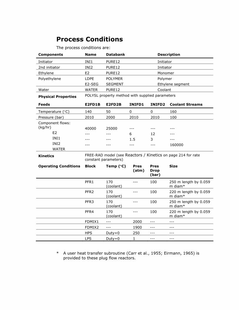
Process Conditions The process conditions are:
Components Name Databank Description
Initiator INI1 PURE12 Initiator
2nd initiator INI2 PURE12 Initiator
Ethylene E2 PURE12 Monomer
Polyethylene LDPE
E2-SEG
POLYMER
SEGMENT
Polymer
Ethylene segment
Water WATER PURE12 Coolant
Physical Properties POLYSL property method with supplied parameters
Feeds E2FD1B E2FD2B INIFD1 INIFD2 Coolant Streams
Temperature (°C) 140 50 0 0 160
Pressure (bar) 2010 2000 2010 2010 100
Component flows: (kg/hr)
E2
INI1
INI2
WATER
40000
---
---
---
25000
---
---
---
---
6
1.5
---
---
12
3
---
---
---
---
160000
Kinetics FREE-RAD model (see Reactors / Kinetics on page 214 for rate constant parameters)
Operating Conditions Block Temp (°C) Pres (atm)
Pres Drop (bar)
Size
PFR1 170 (coolant)
--- 100 250 m length by 0.059 m diam*
PFR2 170 (coolant)
--- 100 220 m length by 0.059 m diam*
PFR3 170 (coolant)
--- 100 250 m length by 0.059 m diam*
PFR4 170 (coolant)
--- 100 220 m length by 0.059 m diam*
FDMIX1 --- 2000 --- ---
FDMIX2 --- 1900 --- ---
HPS Duty=0 250 --- ---
LPS Duty=0 1 --- ---
* A user heat transfer subroutine (Carr et al., 1955; Eirmann, 1965) is provided to these plug flow reactors.
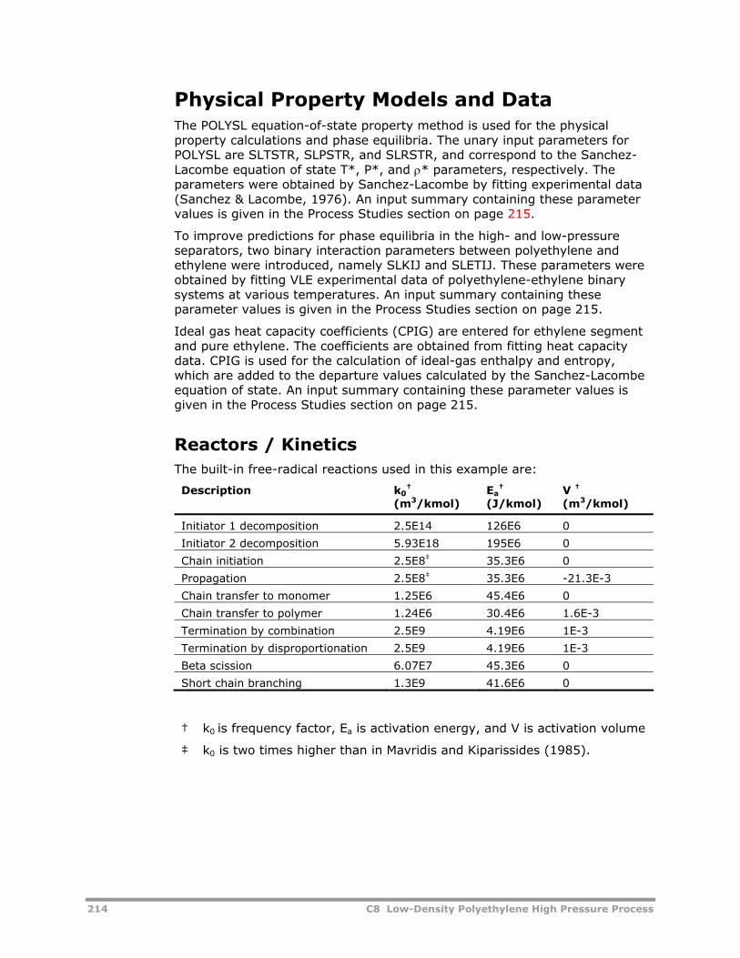
214 C8 Low-Density Polyethylene High Pressure Process
Physical Property Models and Data The POLYSL equation-of-state property method is used for the physical property calculations and phase equilibria. The unary input parameters for POLYSL are SLTSTR, SLPSTR, and SLRSTR, and correspond to the Sanchez-Lacombe equation of state T*, P*, and ρ* parameters, respectively. The parameters were obtained by Sanchez-Lacombe by fitting experimental data (Sanchez & Lacombe, 1976). An input summary containing these parameter values is given in the Process Studies section on page 215.
To improve predictions for phase equilibria in the high- and low-pressure separators, two binary interaction parameters between polyethylene and ethylene were introduced, namely SLKIJ and SLETIJ. These parameters were obtained by fitting VLE experimental data of polyethylene-ethylene binary systems at various temperatures. An input summary containing these parameter values is given in the Process Studies section on page 215.
Ideal gas heat capacity coefficients (CPIG) are entered for ethylene segment and pure ethylene. The coefficients are obtained from fitting heat capacity data. CPIG is used for the calculation of ideal-gas enthalpy and entropy, which are added to the departure values calculated by the Sanchez-Lacombe equation of state. An input summary containing these parameter values is given in the Process Studies section on page 215.
Reactors / Kinetics The built-in free-radical reactions used in this example are:
Description k0†
(m3/kmol) Ea
† (J/kmol)
V † (m3/kmol)
Initiator 1 decomposition 2.5E14 126E6 0
Initiator 2 decomposition 5.93E18 195E6 0
Chain initiation 2.5E8‡ 35.3E6 0
Propagation 2.5E8‡ 35.3E6 -21.3E-3
Chain transfer to monomer 1.25E6 45.4E6 0
Chain transfer to polymer 1.24E6 30.4E6 1.6E-3
Termination by combination 2.5E9 4.19E6 1E-3
Termination by disproportionation 2.5E9 4.19E6 1E-3
Beta scission 6.07E7 45.3E6 0
Short chain branching 1.3E9 41.6E6 0
† k0 is frequency factor, Ea is activation energy, and V is activation volume
‡ k0 is two times higher than in Mavridis and Kiparissides (1985).
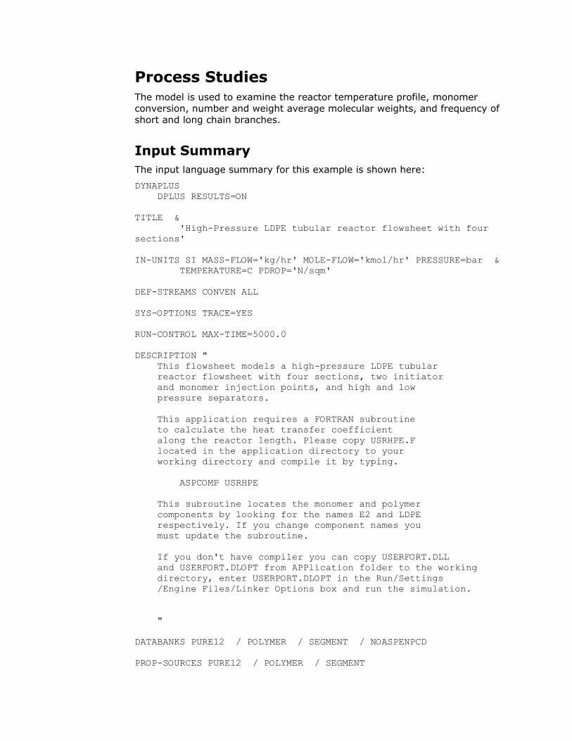
Process Studies The model is used to examine the reactor temperature profile, monomer conversion, number and weight average molecular weights, and frequency of short and long chain branches.
Input Summary The input language summary for this example is shown here:
DYNAPLUS DPLUS RESULTS=ON TITLE & 'High-Pressure LDPE tubular reactor flowsheet with four sections' IN-UNITS SI MASS-FLOW='kg/hr' MOLE-FLOW='kmol/hr' PRESSURE=bar & TEMPERATURE=C PDROP='N/sqm' DEF-STREAMS CONVEN ALL SYS-OPTIONS TRACE=YES RUN-CONTROL MAX-TIME=5000.0 DESCRIPTION " This flowsheet models a high-pressure LDPE tubular reactor flowsheet with four sections, two initiator and monomer injection points, and high and low pressure separators. This application requires a FORTRAN subroutine to calculate the heat transfer coefficient along the reactor length. Please copy USRHPE.F located in the application directory to your working directory and compile it by typing. ASPCOMP USRHPE This subroutine locates the monomer and polymer components by looking for the names E2 and LDPE respectively. If you change component names you must update the subroutine. If you don't have compiler you can copy USERFORT.DLL and USERFORT.DLOPT from APPlication folder to the working directory, enter USERPORT.DLOPT in the Run/Settings /Engine Files/Linker Options box and run the simulation. " DATABANKS PURE12 / POLYMER / SEGMENT / NOASPENPCD PROP-SOURCES PURE12 / POLYMER / SEGMENT
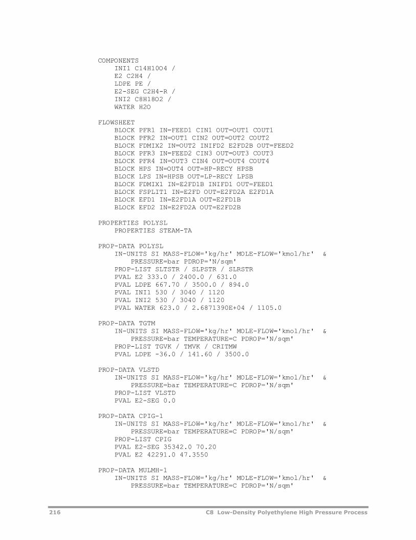
216 C8 Low-Density Polyethylene High Pressure Process
COMPONENTS INI1 C14H10O4 / E2 C2H4 / LDPE PE / E2-SEG C2H4-R / INI2 C8H18O2 / WATER H2O FLOWSHEET BLOCK PFR1 IN=FEED1 CIN1 OUT=OUT1 COUT1 BLOCK PFR2 IN=OUT1 CIN2 OUT=OUT2 COUT2 BLOCK FDMIX2 IN=OUT2 INIFD2 E2FD2B OUT=FEED2 BLOCK PFR3 IN=FEED2 CIN3 OUT=OUT3 COUT3 BLOCK PFR4 IN=OUT3 CIN4 OUT=OUT4 COUT4 BLOCK HPS IN=OUT4 OUT=HP-RECY HPSB BLOCK LPS IN=HPSB OUT=LP-RECY LPSB BLOCK FDMIX1 IN=E2FD1B INIFD1 OUT=FEED1 BLOCK FSPLIT1 IN=E2FD OUT=E2FD2A E2FD1A BLOCK EFD1 IN=E2FD1A OUT=E2FD1B BLOCK EFD2 IN=E2FD2A OUT=E2FD2B PROPERTIES POLYSL PROPERTIES STEAM-TA PROP-DATA POLYSL IN-UNITS SI MASS-FLOW='kg/hr' MOLE-FLOW='kmol/hr' & PRESSURE=bar PDROP='N/sqm' PROP-LIST SLTSTR / SLPSTR / SLRSTR PVAL E2 333.0 / 2400.0 / 631.0 PVAL LDPE 667.70 / 3500.0 / 894.0 PVAL INI1 530 / 3040 / 1120 PVAL INI2 530 / 3040 / 1120 PVAL WATER 623.0 / 2.6871390E+04 / 1105.0 PROP-DATA TGTM IN-UNITS SI MASS-FLOW='kg/hr' MOLE-FLOW='kmol/hr' & PRESSURE=bar TEMPERATURE=C PDROP='N/sqm' PROP-LIST TGVK / TMVK / CRITMW PVAL LDPE -36.0 / 141.60 / 3500.0 PROP-DATA VLSTD IN-UNITS SI MASS-FLOW='kg/hr' MOLE-FLOW='kmol/hr' & PRESSURE=bar TEMPERATURE=C PDROP='N/sqm' PROP-LIST VLSTD PVAL E2-SEG 0.0 PROP-DATA CPIG-1 IN-UNITS SI MASS-FLOW='kg/hr' MOLE-FLOW='kmol/hr' & PRESSURE=bar TEMPERATURE=C PDROP='N/sqm' PROP-LIST CPIG PVAL E2-SEG 35342.0 70.20 PVAL E2 42291.0 47.3550 PROP-DATA MULMH-1 IN-UNITS SI MASS-FLOW='kg/hr' MOLE-FLOW='kmol/hr' & PRESSURE=bar TEMPERATURE=C PDROP='N/sqm'
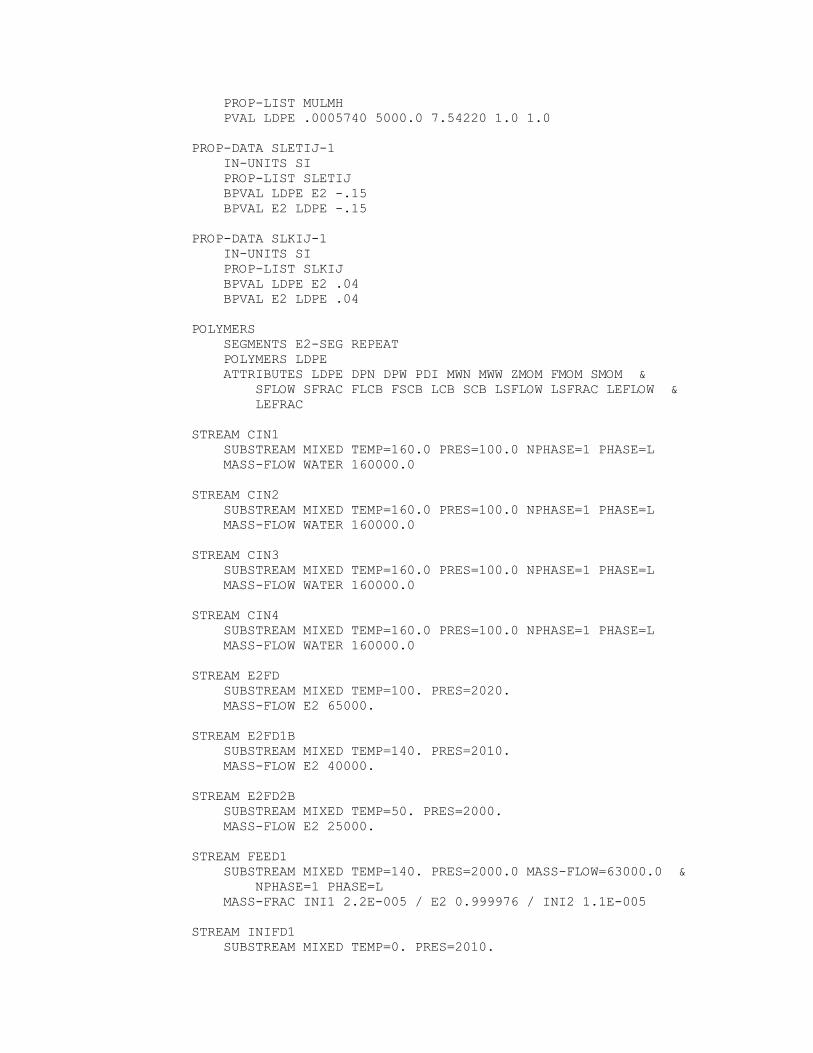
PROP-LIST MULMH PVAL LDPE .0005740 5000.0 7.54220 1.0 1.0 PROP-DATA SLETIJ-1 IN-UNITS SI PROP-LIST SLETIJ BPVAL LDPE E2 -.15 BPVAL E2 LDPE -.15 PROP-DATA SLKIJ-1 IN-UNITS SI PROP-LIST SLKIJ BPVAL LDPE E2 .04 BPVAL E2 LDPE .04 POLYMERS SEGMENTS E2-SEG REPEAT POLYMERS LDPE ATTRIBUTES LDPE DPN DPW PDI MWN MWW ZMOM FMOM SMOM & SFLOW SFRAC FLCB FSCB LCB SCB LSFLOW LSFRAC LEFLOW & LEFRAC STREAM CIN1 SUBSTREAM MIXED TEMP=160.0 PRES=100.0 NPHASE=1 PHASE=L MASS-FLOW WATER 160000.0 STREAM CIN2 SUBSTREAM MIXED TEMP=160.0 PRES=100.0 NPHASE=1 PHASE=L MASS-FLOW WATER 160000.0 STREAM CIN3 SUBSTREAM MIXED TEMP=160.0 PRES=100.0 NPHASE=1 PHASE=L MASS-FLOW WATER 160000.0 STREAM CIN4 SUBSTREAM MIXED TEMP=160.0 PRES=100.0 NPHASE=1 PHASE=L MASS-FLOW WATER 160000.0 STREAM E2FD SUBSTREAM MIXED TEMP=100. PRES=2020. MASS-FLOW E2 65000. STREAM E2FD1B SUBSTREAM MIXED TEMP=140. PRES=2010. MASS-FLOW E2 40000. STREAM E2FD2B SUBSTREAM MIXED TEMP=50. PRES=2000. MASS-FLOW E2 25000. STREAM FEED1 SUBSTREAM MIXED TEMP=140. PRES=2000.0 MASS-FLOW=63000.0 & NPHASE=1 PHASE=L MASS-FRAC INI1 2.2E-005 / E2 0.999976 / INI2 1.1E-005 STREAM INIFD1 SUBSTREAM MIXED TEMP=0. PRES=2010.
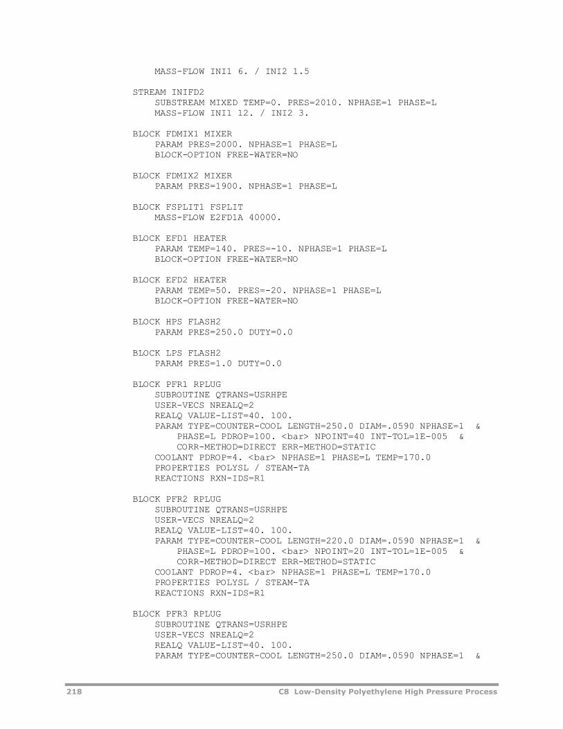
218 C8 Low-Density Polyethylene High Pressure Process
MASS-FLOW INI1 6. / INI2 1.5 STREAM INIFD2 SUBSTREAM MIXED TEMP=0. PRES=2010. NPHASE=1 PHASE=L MASS-FLOW INI1 12. / INI2 3. BLOCK FDMIX1 MIXER PARAM PRES=2000. NPHASE=1 PHASE=L BLOCK-OPTION FREE-WATER=NO BLOCK FDMIX2 MIXER PARAM PRES=1900. NPHASE=1 PHASE=L BLOCK FSPLIT1 FSPLIT MASS-FLOW E2FD1A 40000. BLOCK EFD1 HEATER PARAM TEMP=140. PRES=-10. NPHASE=1 PHASE=L BLOCK-OPTION FREE-WATER=NO BLOCK EFD2 HEATER PARAM TEMP=50. PRES=-20. NPHASE=1 PHASE=L BLOCK-OPTION FREE-WATER=NO BLOCK HPS FLASH2 PARAM PRES=250.0 DUTY=0.0 BLOCK LPS FLASH2 PARAM PRES=1.0 DUTY=0.0 BLOCK PFR1 RPLUG SUBROUTINE QTRANS=USRHPE USER-VECS NREALQ=2 REALQ VALUE-LIST=40. 100. PARAM TYPE=COUNTER-COOL LENGTH=250.0 DIAM=.0590 NPHASE=1 & PHASE=L PDROP=100. <bar> NPOINT=40 INT-TOL=1E-005 & CORR-METHOD=DIRECT ERR-METHOD=STATIC COOLANT PDROP=4. <bar> NPHASE=1 PHASE=L TEMP=170.0 PROPERTIES POLYSL / STEAM-TA REACTIONS RXN-IDS=R1 BLOCK PFR2 RPLUG SUBROUTINE QTRANS=USRHPE USER-VECS NREALQ=2 REALQ VALUE-LIST=40. 100. PARAM TYPE=COUNTER-COOL LENGTH=220.0 DIAM=.0590 NPHASE=1 & PHASE=L PDROP=100. <bar> NPOINT=20 INT-TOL=1E-005 & CORR-METHOD=DIRECT ERR-METHOD=STATIC COOLANT PDROP=4. <bar> NPHASE=1 PHASE=L TEMP=170.0 PROPERTIES POLYSL / STEAM-TA REACTIONS RXN-IDS=R1 BLOCK PFR3 RPLUG SUBROUTINE QTRANS=USRHPE USER-VECS NREALQ=2 REALQ VALUE-LIST=40. 100. PARAM TYPE=COUNTER-COOL LENGTH=250.0 DIAM=.0590 NPHASE=1 &
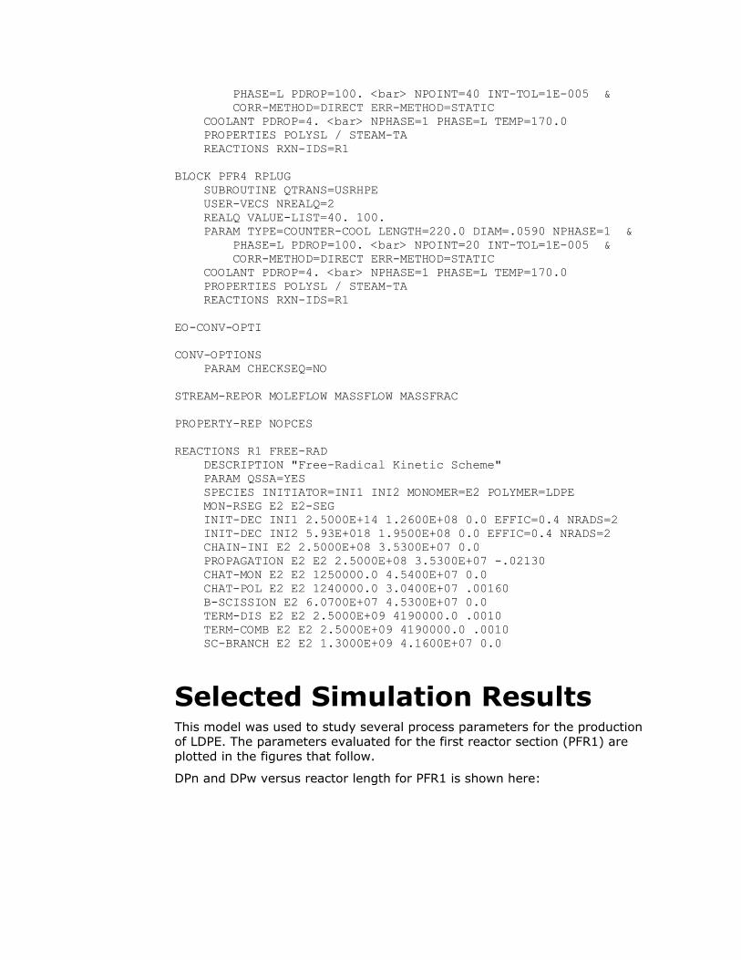
PHASE=L PDROP=100. <bar> NPOINT=40 INT-TOL=1E-005 & CORR-METHOD=DIRECT ERR-METHOD=STATIC COOLANT PDROP=4. <bar> NPHASE=1 PHASE=L TEMP=170.0 PROPERTIES POLYSL / STEAM-TA REACTIONS RXN-IDS=R1 BLOCK PFR4 RPLUG SUBROUTINE QTRANS=USRHPE USER-VECS NREALQ=2 REALQ VALUE-LIST=40. 100. PARAM TYPE=COUNTER-COOL LENGTH=220.0 DIAM=.0590 NPHASE=1 & PHASE=L PDROP=100. <bar> NPOINT=20 INT-TOL=1E-005 & CORR-METHOD=DIRECT ERR-METHOD=STATIC COOLANT PDROP=4. <bar> NPHASE=1 PHASE=L TEMP=170.0 PROPERTIES POLYSL / STEAM-TA REACTIONS RXN-IDS=R1 EO-CONV-OPTI CONV-OPTIONS PARAM CHECKSEQ=NO STREAM-REPOR MOLEFLOW MASSFLOW MASSFRAC PROPERTY-REP NOPCES REACTIONS R1 FREE-RAD DESCRIPTION "Free-Radical Kinetic Scheme" PARAM QSSA=YES SPECIES INITIATOR=INI1 INI2 MONOMER=E2 POLYMER=LDPE MON-RSEG E2 E2-SEG INIT-DEC INI1 2.5000E+14 1.2600E+08 0.0 EFFIC=0.4 NRADS=2 INIT-DEC INI2 5.93E+018 1.9500E+08 0.0 EFFIC=0.4 NRADS=2 CHAIN-INI E2 2.5000E+08 3.5300E+07 0.0 PROPAGATION E2 E2 2.5000E+08 3.5300E+07 -.02130 CHAT-MON E2 E2 1250000.0 4.5400E+07 0.0 CHAT-POL E2 E2 1240000.0 3.0400E+07 .00160 B-SCISSION E2 6.0700E+07 4.5300E+07 0.0 TERM-DIS E2 E2 2.5000E+09 4190000.0 .0010 TERM-COMB E2 E2 2.5000E+09 4190000.0 .0010 SC-BRANCH E2 E2 1.3000E+09 4.1600E+07 0.0
Selected Simulation Results This model was used to study several process parameters for the production of LDPE. The parameters evaluated for the first reactor section (PFR1) are plotted in the figures that follow.
DPn and DPw versus reactor length for PFR1 is shown here:
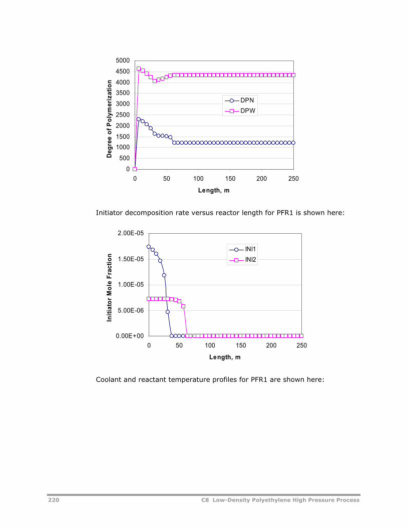
220 C8 Low-Density Polyethylene High Pressure Process
0
500
10001500
2000
2500
3000
35004000
4500
5000
0 50 100 150 200 250
Length, m
Degr
ee o
f Pol
ymer
izat
ion
DPNDPW
Initiator decomposition rate versus reactor length for PFR1 is shown here:
0.00E+00
5.00E-06
1.00E-05
1.50E-05
2.00E-05
0 50 100 150 200 250
Length, m
Initi
ator
Mol
e Fr
actio
n
INI1INI2
Coolant and reactant temperature profiles for PFR1 are shown here:
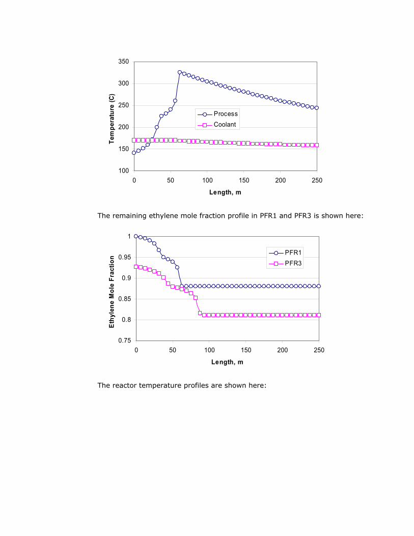
100
150
200
250
300
350
0 50 100 150 200 250
Length, m
Tem
pera
ture
(C)
ProcessCoolant
The remaining ethylene mole fraction profile in PFR1 and PFR3 is shown here:
0.75
0.8
0.85
0.9
0.95
1
0 50 100 150 200 250
Length, m
Ethy
lene
Mol
e Fr
actio
n
PFR1PFR3
The reactor temperature profiles are shown here:
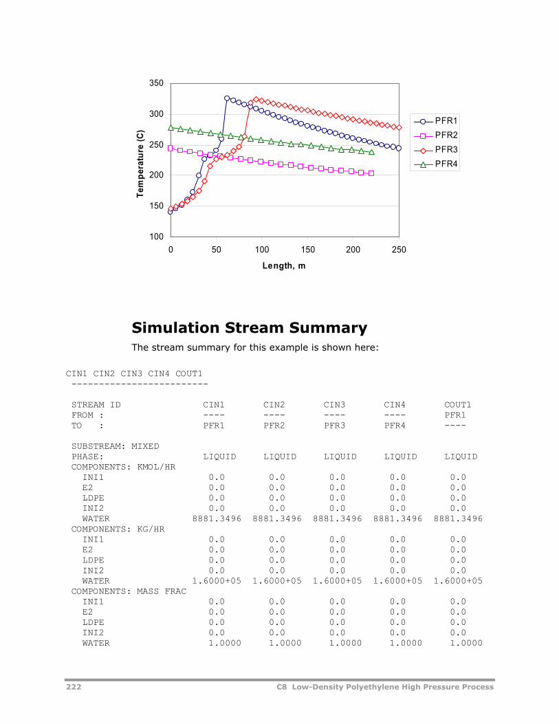
222 C8 Low-Density Polyethylene High Pressure Process
100
150
200
250
300
350
0 50 100 150 200 250
Length, m
Tem
pera
ture
(C)
PFR1PFR2PFR3PFR4
Simulation Stream Summary The stream summary for this example is shown here:
CIN1 CIN2 CIN3 CIN4 COUT1 ------------------------- STREAM ID CIN1 CIN2 CIN3 CIN4 COUT1 FROM : ---- ---- ---- ---- PFR1 TO : PFR1 PFR2 PFR3 PFR4 ---- SUBSTREAM: MIXED PHASE: LIQUID LIQUID LIQUID LIQUID LIQUID COMPONENTS: KMOL/HR INI1 0.0 0.0 0.0 0.0 0.0 E2 0.0 0.0 0.0 0.0 0.0 LDPE 0.0 0.0 0.0 0.0 0.0 INI2 0.0 0.0 0.0 0.0 0.0 WATER 8881.3496 8881.3496 8881.3496 8881.3496 8881.3496 COMPONENTS: KG/HR INI1 0.0 0.0 0.0 0.0 0.0 E2 0.0 0.0 0.0 0.0 0.0 LDPE 0.0 0.0 0.0 0.0 0.0 INI2 0.0 0.0 0.0 0.0 0.0 WATER 1.6000+05 1.6000+05 1.6000+05 1.6000+05 1.6000+05 COMPONENTS: MASS FRAC INI1 0.0 0.0 0.0 0.0 0.0 E2 0.0 0.0 0.0 0.0 0.0 LDPE 0.0 0.0 0.0 0.0 0.0 INI2 0.0 0.0 0.0 0.0 0.0 WATER 1.0000 1.0000 1.0000 1.0000 1.0000
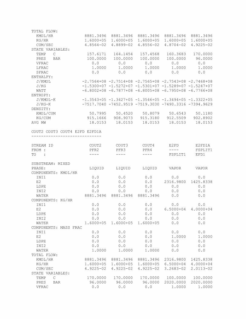
TOTAL FLOW: KMOL/HR 8881.3496 8881.3496 8881.3496 8881.3496 8881.3496 KG/HR 1.6000+05 1.6000+05 1.6000+05 1.6000+05 1.6000+05 CUM/SEC 4.8564-02 4.8899-02 4.8556-02 4.8704-02 4.9225-02 STATE VARIABLES: TEMP C 157.6171 164.1454 157.4568 160.3683 170.0000 PRES BAR 100.0000 100.0000 100.0000 100.0000 96.0000 VFRAC 0.0 0.0 0.0 0.0 0.0 LFRAC 1.0000 1.0000 1.0000 1.0000 1.0000 SFRAC 0.0 0.0 0.0 0.0 0.0 ENTHALPY: J/KMOL -2.7564+08 -2.7514+08 -2.7565+08 -2.7543+08 -2.7468+08 J/KG -1.5300+07 -1.5272+07 -1.5301+07 -1.5289+07 -1.5247+07 WATT -6.8002+08 -6.7877+08 -6.8005+08 -6.7950+08 -6.7766+08 ENTROPY: J/KMOL-K -1.3543+05 -1.3427+05 -1.3546+05 -1.3494+05 -1.3322+05 J/KG-K -7517.7040 -7452.9519 -7519.3030 -7490.3316 -7394.9629 DENSITY: KMOL/CUM 50.7995 50.4520 50.8079 50.6543 50.1180 KG/CUM 915.1666 908.9073 915.3180 912.5509 902.8902 AVG MW 18.0153 18.0153 18.0153 18.0153 18.0153 COUT2 COUT3 COUT4 E2FD E2FD1A ----------------------------- STREAM ID COUT2 COUT3 COUT4 E2FD E2FD1A FROM : PFR2 PFR3 PFR4 ---- FSPLIT1 TO : ---- ---- ---- FSPLIT1 EFD1 SUBSTREAM: MIXED PHASE: LIQUID LIQUID LIQUID VAPOR VAPOR COMPONENTS: KMOL/HR INI1 0.0 0.0 0.0 0.0 0.0 E2 0.0 0.0 0.0 2316.9800 1425.8338 LDPE 0.0 0.0 0.0 0.0 0.0 INI2 0.0 0.0 0.0 0.0 0.0 WATER 8881.3496 8881.3496 8881.3496 0.0 0.0 COMPONENTS: KG/HR INI1 0.0 0.0 0.0 0.0 0.0 E2 0.0 0.0 0.0 6.5000+04 4.0000+04 LDPE 0.0 0.0 0.0 0.0 0.0 INI2 0.0 0.0 0.0 0.0 0.0 WATER 1.6000+05 1.6000+05 1.6000+05 0.0 0.0 COMPONENTS: MASS FRAC INI1 0.0 0.0 0.0 0.0 0.0 E2 0.0 0.0 0.0 1.0000 1.0000 LDPE 0.0 0.0 0.0 0.0 0.0 INI2 0.0 0.0 0.0 0.0 0.0 WATER 1.0000 1.0000 1.0000 0.0 0.0 TOTAL FLOW: KMOL/HR 8881.3496 8881.3496 8881.3496 2316.9800 1425.8338 KG/HR 1.6000+05 1.6000+05 1.6000+05 6.5000+04 4.0000+04 CUM/SEC 4.9225-02 4.9225-02 4.9225-02 3.2683-02 2.0113-02 STATE VARIABLES: TEMP C 170.0000 170.0000 170.0000 100.0000 100.0000 PRES BAR 96.0000 96.0000 96.0000 2020.0000 2020.0000 VFRAC 0.0 0.0 0.0 1.0000 1.0000
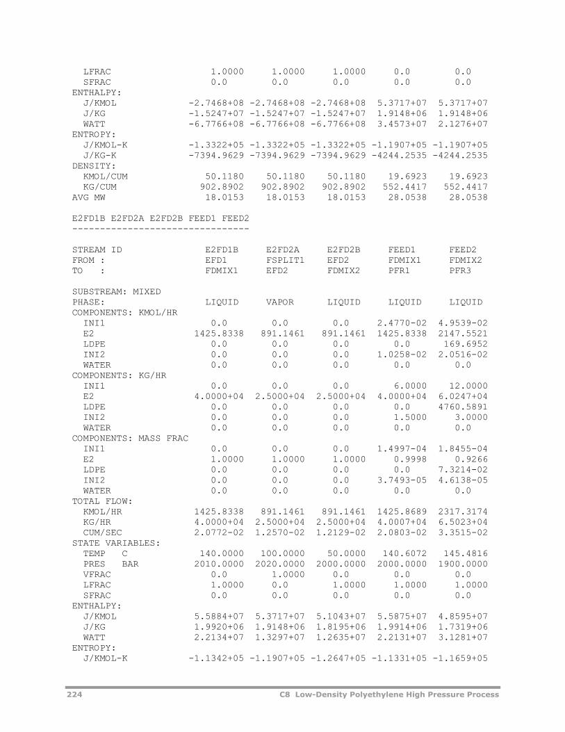
224 C8 Low-Density Polyethylene High Pressure Process
LFRAC 1.0000 1.0000 1.0000 0.0 0.0 SFRAC 0.0 0.0 0.0 0.0 0.0 ENTHALPY: J/KMOL -2.7468+08 -2.7468+08 -2.7468+08 5.3717+07 5.3717+07 J/KG -1.5247+07 -1.5247+07 -1.5247+07 1.9148+06 1.9148+06 WATT -6.7766+08 -6.7766+08 -6.7766+08 3.4573+07 2.1276+07 ENTROPY: J/KMOL-K -1.3322+05 -1.3322+05 -1.3322+05 -1.1907+05 -1.1907+05 J/KG-K -7394.9629 -7394.9629 -7394.9629 -4244.2535 -4244.2535 DENSITY: KMOL/CUM 50.1180 50.1180 50.1180 19.6923 19.6923 KG/CUM 902.8902 902.8902 902.8902 552.4417 552.4417 AVG MW 18.0153 18.0153 18.0153 28.0538 28.0538 E2FD1B E2FD2A E2FD2B FEED1 FEED2 -------------------------------- STREAM ID E2FD1B E2FD2A E2FD2B FEED1 FEED2 FROM : EFD1 FSPLIT1 EFD2 FDMIX1 FDMIX2 TO : FDMIX1 EFD2 FDMIX2 PFR1 PFR3 SUBSTREAM: MIXED PHASE: LIQUID VAPOR LIQUID LIQUID LIQUID COMPONENTS: KMOL/HR INI1 0.0 0.0 0.0 2.4770-02 4.9539-02 E2 1425.8338 891.1461 891.1461 1425.8338 2147.5521 LDPE 0.0 0.0 0.0 0.0 169.6952 INI2 0.0 0.0 0.0 1.0258-02 2.0516-02 WATER 0.0 0.0 0.0 0.0 0.0 COMPONENTS: KG/HR INI1 0.0 0.0 0.0 6.0000 12.0000 E2 4.0000+04 2.5000+04 2.5000+04 4.0000+04 6.0247+04 LDPE 0.0 0.0 0.0 0.0 4760.5891 INI2 0.0 0.0 0.0 1.5000 3.0000 WATER 0.0 0.0 0.0 0.0 0.0 COMPONENTS: MASS FRAC INI1 0.0 0.0 0.0 1.4997-04 1.8455-04 E2 1.0000 1.0000 1.0000 0.9998 0.9266 LDPE 0.0 0.0 0.0 0.0 7.3214-02 INI2 0.0 0.0 0.0 3.7493-05 4.6138-05 WATER 0.0 0.0 0.0 0.0 0.0 TOTAL FLOW: KMOL/HR 1425.8338 891.1461 891.1461 1425.8689 2317.3174 KG/HR 4.0000+04 2.5000+04 2.5000+04 4.0007+04 6.5023+04 CUM/SEC 2.0772-02 1.2570-02 1.2129-02 2.0803-02 3.3515-02 STATE VARIABLES: TEMP C 140.0000 100.0000 50.0000 140.6072 145.4816 PRES BAR 2010.0000 2020.0000 2000.0000 2000.0000 1900.0000 VFRAC 0.0 1.0000 0.0 0.0 0.0 LFRAC 1.0000 0.0 1.0000 1.0000 1.0000 SFRAC 0.0 0.0 0.0 0.0 0.0 ENTHALPY: J/KMOL 5.5884+07 5.3717+07 5.1043+07 5.5875+07 4.8595+07 J/KG 1.9920+06 1.9148+06 1.8195+06 1.9914+06 1.7319+06 WATT 2.2134+07 1.3297+07 1.2635+07 2.2131+07 3.1281+07 ENTROPY: J/KMOL-K -1.1342+05 -1.1907+05 -1.2647+05 -1.1331+05 -1.1659+05
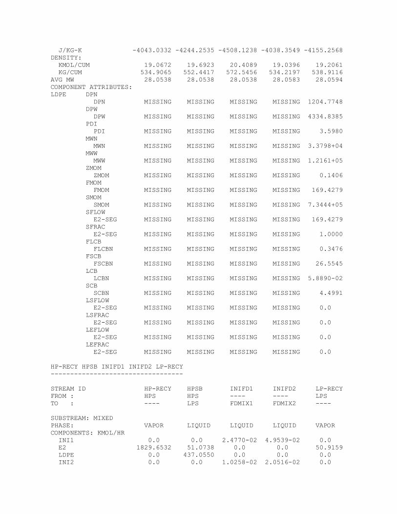
J/KG-K -4043.0332 -4244.2535 -4508.1238 -4038.3549 -4155.2568 DENSITY: KMOL/CUM 19.0672 19.6923 20.4089 19.0396 19.2061 KG/CUM 534.9065 552.4417 572.5456 534.2197 538.9116 AVG MW 28.0538 28.0538 28.0538 28.0583 28.0594 COMPONENT ATTRIBUTES: LDPE DPN DPN MISSING MISSING MISSING MISSING 1204.7748 DPW DPW MISSING MISSING MISSING MISSING 4334.8385 PDI PDI MISSING MISSING MISSING MISSING 3.5980 MWN MWN MISSING MISSING MISSING MISSING 3.3798+04 MWW MWW MISSING MISSING MISSING MISSING 1.2161+05 ZMOM ZMOM MISSING MISSING MISSING MISSING 0.1406 FMOM FMOM MISSING MISSING MISSING MISSING 169.4279 SMOM SMOM MISSING MISSING MISSING MISSING 7.3444+05 SFLOW E2-SEG MISSING MISSING MISSING MISSING 169.4279 SFRAC E2-SEG MISSING MISSING MISSING MISSING 1.0000 FLCB FLCBN MISSING MISSING MISSING MISSING 0.3476 FSCB FSCBN MISSING MISSING MISSING MISSING 26.5545 LCB LCBN MISSING MISSING MISSING MISSING 5.8890-02 SCB SCBN MISSING MISSING MISSING MISSING 4.4991 LSFLOW E2-SEG MISSING MISSING MISSING MISSING 0.0 LSFRAC E2-SEG MISSING MISSING MISSING MISSING 0.0 LEFLOW E2-SEG MISSING MISSING MISSING MISSING 0.0 LEFRAC E2-SEG MISSING MISSING MISSING MISSING 0.0 HP-RECY HPSB INIFD1 INIFD2 LP-RECY ---------------------------------- STREAM ID HP-RECY HPSB INIFD1 INIFD2 LP-RECY FROM : HPS HPS ---- ---- LPS TO : ---- LPS FDMIX1 FDMIX2 ---- SUBSTREAM: MIXED PHASE: VAPOR LIQUID LIQUID LIQUID VAPOR COMPONENTS: KMOL/HR INI1 0.0 0.0 2.4770-02 4.9539-02 0.0 E2 1829.6532 51.0738 0.0 0.0 50.9159 LDPE 0.0 437.0550 0.0 0.0 0.0 INI2 0.0 0.0 1.0258-02 2.0516-02 0.0
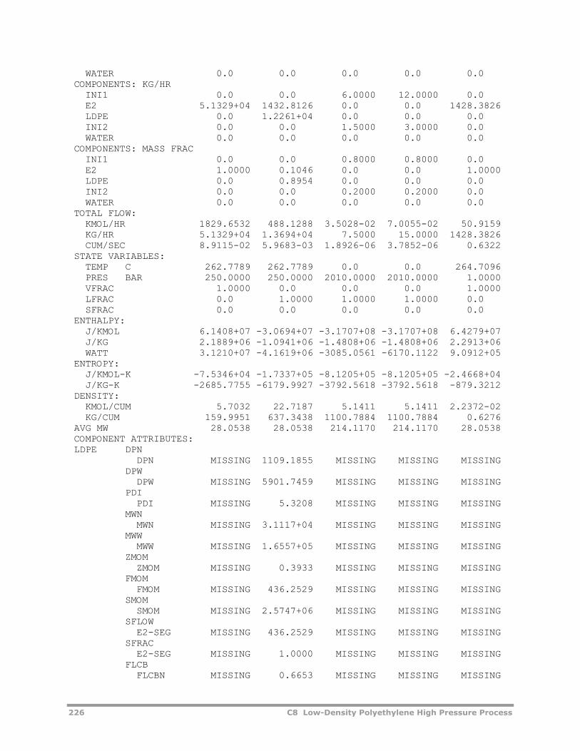
226 C8 Low-Density Polyethylene High Pressure Process
WATER 0.0 0.0 0.0 0.0 0.0 COMPONENTS: KG/HR INI1 0.0 0.0 6.0000 12.0000 0.0 E2 5.1329+04 1432.8126 0.0 0.0 1428.3826 LDPE 0.0 1.2261+04 0.0 0.0 0.0 INI2 0.0 0.0 1.5000 3.0000 0.0 WATER 0.0 0.0 0.0 0.0 0.0 COMPONENTS: MASS FRAC INI1 0.0 0.0 0.8000 0.8000 0.0 E2 1.0000 0.1046 0.0 0.0 1.0000 LDPE 0.0 0.8954 0.0 0.0 0.0 INI2 0.0 0.0 0.2000 0.2000 0.0 WATER 0.0 0.0 0.0 0.0 0.0 TOTAL FLOW: KMOL/HR 1829.6532 488.1288 3.5028-02 7.0055-02 50.9159 KG/HR 5.1329+04 1.3694+04 7.5000 15.0000 1428.3826 CUM/SEC 8.9115-02 5.9683-03 1.8926-06 3.7852-06 0.6322 STATE VARIABLES: TEMP C 262.7789 262.7789 0.0 0.0 264.7096 PRES BAR 250.0000 250.0000 2010.0000 2010.0000 1.0000 VFRAC 1.0000 0.0 0.0 0.0 1.0000 LFRAC 0.0 1.0000 1.0000 1.0000 0.0 SFRAC 0.0 0.0 0.0 0.0 0.0 ENTHALPY: J/KMOL 6.1408+07 -3.0694+07 -3.1707+08 -3.1707+08 6.4279+07 J/KG 2.1889+06 -1.0941+06 -1.4808+06 -1.4808+06 2.2913+06 WATT 3.1210+07 -4.1619+06 -3085.0561 -6170.1122 9.0912+05 ENTROPY: J/KMOL-K -7.5346+04 -1.7337+05 -8.1205+05 -8.1205+05 -2.4668+04 J/KG-K -2685.7755 -6179.9927 -3792.5618 -3792.5618 -879.3212 DENSITY: KMOL/CUM 5.7032 22.7187 5.1411 5.1411 2.2372-02 KG/CUM 159.9951 637.3438 1100.7884 1100.7884 0.6276 AVG MW 28.0538 28.0538 214.1170 214.1170 28.0538 COMPONENT ATTRIBUTES: LDPE DPN DPN MISSING 1109.1855 MISSING MISSING MISSING DPW DPW MISSING 5901.7459 MISSING MISSING MISSING PDI PDI MISSING 5.3208 MISSING MISSING MISSING MWN MWN MISSING 3.1117+04 MISSING MISSING MISSING MWW MWW MISSING 1.6557+05 MISSING MISSING MISSING ZMOM ZMOM MISSING 0.3933 MISSING MISSING MISSING FMOM FMOM MISSING 436.2529 MISSING MISSING MISSING SMOM SMOM MISSING 2.5747+06 MISSING MISSING MISSING SFLOW E2-SEG MISSING 436.2529 MISSING MISSING MISSING SFRAC E2-SEG MISSING 1.0000 MISSING MISSING MISSING FLCB FLCBN MISSING 0.6653 MISSING MISSING MISSING
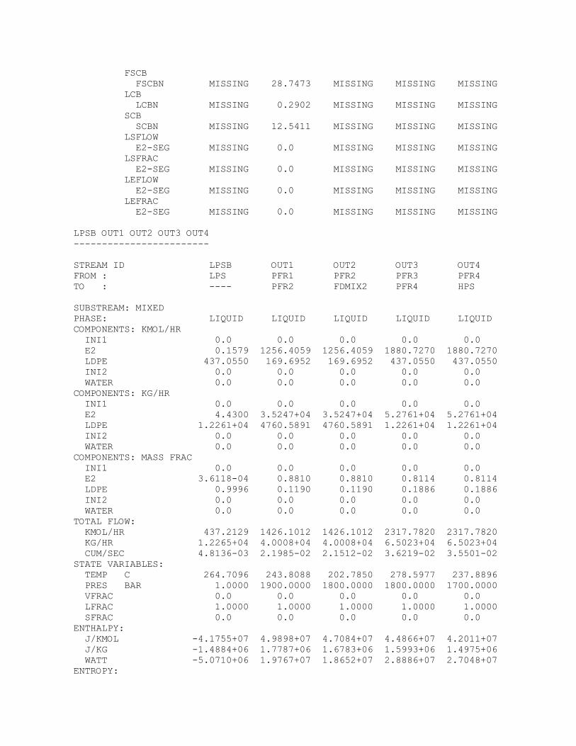
FSCB FSCBN MISSING 28.7473 MISSING MISSING MISSING LCB LCBN MISSING 0.2902 MISSING MISSING MISSING SCB SCBN MISSING 12.5411 MISSING MISSING MISSING LSFLOW E2-SEG MISSING 0.0 MISSING MISSING MISSING LSFRAC E2-SEG MISSING 0.0 MISSING MISSING MISSING LEFLOW E2-SEG MISSING 0.0 MISSING MISSING MISSING LEFRAC E2-SEG MISSING 0.0 MISSING MISSING MISSING LPSB OUT1 OUT2 OUT3 OUT4 ------------------------ STREAM ID LPSB OUT1 OUT2 OUT3 OUT4 FROM : LPS PFR1 PFR2 PFR3 PFR4 TO : ---- PFR2 FDMIX2 PFR4 HPS SUBSTREAM: MIXED PHASE: LIQUID LIQUID LIQUID LIQUID LIQUID COMPONENTS: KMOL/HR INI1 0.0 0.0 0.0 0.0 0.0 E2 0.1579 1256.4059 1256.4059 1880.7270 1880.7270 LDPE 437.0550 169.6952 169.6952 437.0550 437.0550 INI2 0.0 0.0 0.0 0.0 0.0 WATER 0.0 0.0 0.0 0.0 0.0 COMPONENTS: KG/HR INI1 0.0 0.0 0.0 0.0 0.0 E2 4.4300 3.5247+04 3.5247+04 5.2761+04 5.2761+04 LDPE 1.2261+04 4760.5891 4760.5891 1.2261+04 1.2261+04 INI2 0.0 0.0 0.0 0.0 0.0 WATER 0.0 0.0 0.0 0.0 0.0 COMPONENTS: MASS FRAC INI1 0.0 0.0 0.0 0.0 0.0 E2 3.6118-04 0.8810 0.8810 0.8114 0.8114 LDPE 0.9996 0.1190 0.1190 0.1886 0.1886 INI2 0.0 0.0 0.0 0.0 0.0 WATER 0.0 0.0 0.0 0.0 0.0 TOTAL FLOW: KMOL/HR 437.2129 1426.1012 1426.1012 2317.7820 2317.7820 KG/HR 1.2265+04 4.0008+04 4.0008+04 6.5023+04 6.5023+04 CUM/SEC 4.8136-03 2.1985-02 2.1512-02 3.6219-02 3.5501-02 STATE VARIABLES: TEMP C 264.7096 243.8088 202.7850 278.5977 237.8896 PRES BAR 1.0000 1900.0000 1800.0000 1800.0000 1700.0000 VFRAC 0.0 0.0 0.0 0.0 0.0 LFRAC 1.0000 1.0000 1.0000 1.0000 1.0000 SFRAC 0.0 0.0 0.0 0.0 0.0 ENTHALPY: J/KMOL -4.1755+07 4.9898+07 4.7084+07 4.4866+07 4.2011+07 J/KG -1.4884+06 1.7787+06 1.6783+06 1.5993+06 1.4975+06 WATT -5.0710+06 1.9767+07 1.8652+07 2.8886+07 2.7048+07 ENTROPY:
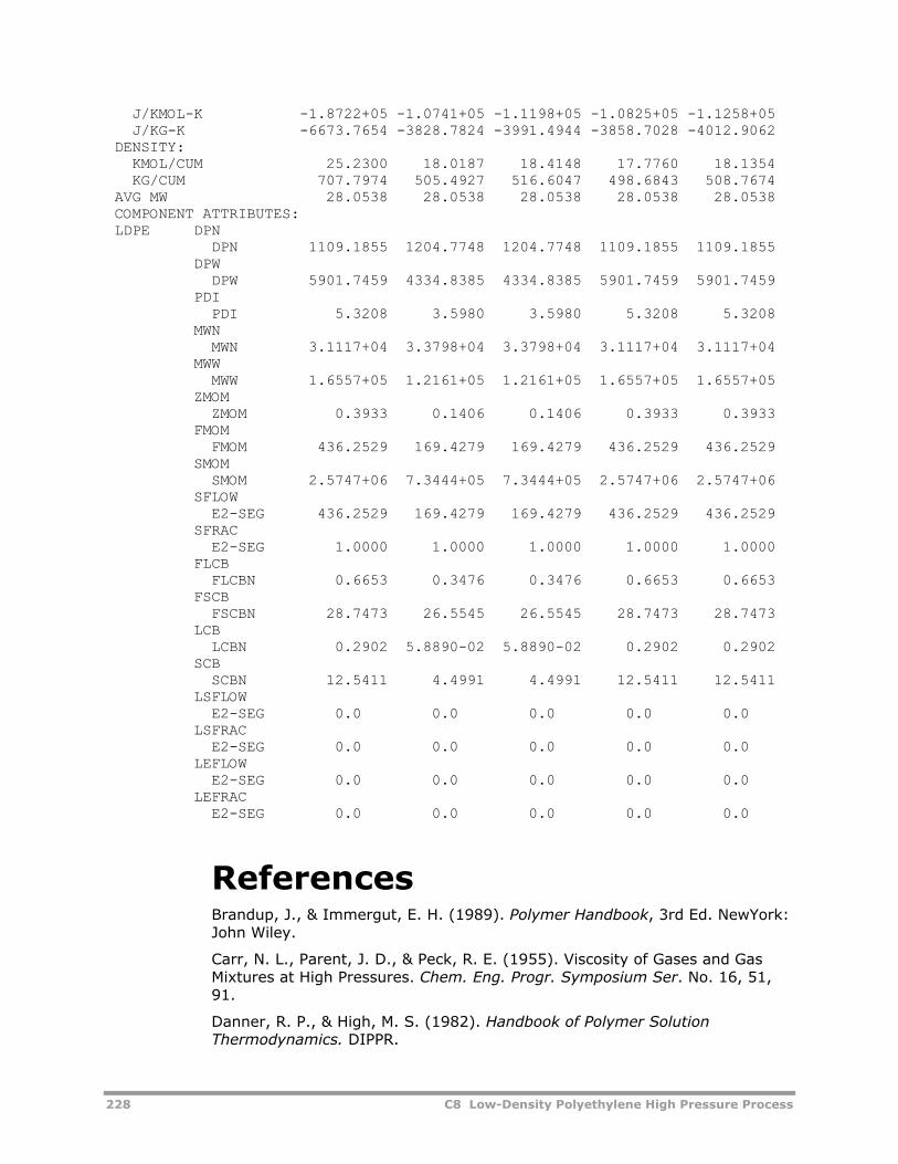
228 C8 Low-Density Polyethylene High Pressure Process
J/KMOL-K -1.8722+05 -1.0741+05 -1.1198+05 -1.0825+05 -1.1258+05 J/KG-K -6673.7654 -3828.7824 -3991.4944 -3858.7028 -4012.9062 DENSITY: KMOL/CUM 25.2300 18.0187 18.4148 17.7760 18.1354 KG/CUM 707.7974 505.4927 516.6047 498.6843 508.7674 AVG MW 28.0538 28.0538 28.0538 28.0538 28.0538 COMPONENT ATTRIBUTES: LDPE DPN DPN 1109.1855 1204.7748 1204.7748 1109.1855 1109.1855 DPW DPW 5901.7459 4334.8385 4334.8385 5901.7459 5901.7459 PDI PDI 5.3208 3.5980 3.5980 5.3208 5.3208 MWN MWN 3.1117+04 3.3798+04 3.3798+04 3.1117+04 3.1117+04 MWW MWW 1.6557+05 1.2161+05 1.2161+05 1.6557+05 1.6557+05 ZMOM ZMOM 0.3933 0.1406 0.1406 0.3933 0.3933 FMOM FMOM 436.2529 169.4279 169.4279 436.2529 436.2529 SMOM SMOM 2.5747+06 7.3444+05 7.3444+05 2.5747+06 2.5747+06 SFLOW E2-SEG 436.2529 169.4279 169.4279 436.2529 436.2529 SFRAC E2-SEG 1.0000 1.0000 1.0000 1.0000 1.0000 FLCB FLCBN 0.6653 0.3476 0.3476 0.6653 0.6653 FSCB FSCBN 28.7473 26.5545 26.5545 28.7473 28.7473 LCB LCBN 0.2902 5.8890-02 5.8890-02 0.2902 0.2902 SCB SCBN 12.5411 4.4991 4.4991 12.5411 12.5411 LSFLOW E2-SEG 0.0 0.0 0.0 0.0 0.0 LSFRAC E2-SEG 0.0 0.0 0.0 0.0 0.0 LEFLOW E2-SEG 0.0 0.0 0.0 0.0 0.0 LEFRAC E2-SEG 0.0 0.0 0.0 0.0 0.0
References Brandup, J., & Immergut, E. H. (1989). Polymer Handbook, 3rd Ed. NewYork: John Wiley.
Carr, N. L., Parent, J. D., & Peck, R. E. (1955). Viscosity of Gases and Gas Mixtures at High Pressures. Chem. Eng. Progr. Symposium Ser. No. 16, 51, 91.
Danner, R. P., & High, M. S. (1982). Handbook of Polymer Solution Thermodynamics. DIPPR.
Eirmann, K. (1965). Modellmässige Deutung de Wärmeleitfahigkeit von Hochpolymeren. Koll. Z., 201, p. 3.
Hellwege, K. H., Knoppf, W., & Wetzel, W. (1962). Spezifische Wäarme von Polyolefinen und einigen anderen Hochpolymeren im Temperaturbereich von 300°C - 180°C. Koll. Z., 180, p. 126.
Mavridis, I., & Kiparissides, C. (1985). Optimization of a High-Pressure Polyethylene Tubular Reactor. Polymer Process Engineering, 3(3), pp. 263-290.
Michels, A., & Geldermans, M. (1942). Isotherms of Ethylene Up to 3,000 Atmospheres Between 0°C and 150°C. Physica, 9, p. 967.
Odian, G. (1991). Principles of Polymerization, 3rd Ed. New York: John Wiley and Sons.
Sanchez, I. C., & Lacombe, R. H. (1976). An Elementary Molecular Theory of Chemical Fluids. Pure Fluids. J. Phys. Chem., 80(21), pp. 2352-2362.
Sanchez, I. C., & Lacombe, R. H. (1978). Statistical Thermodynamics of Polymer Solutions. Macromolecules, 11(6), pp. 1145-1156.
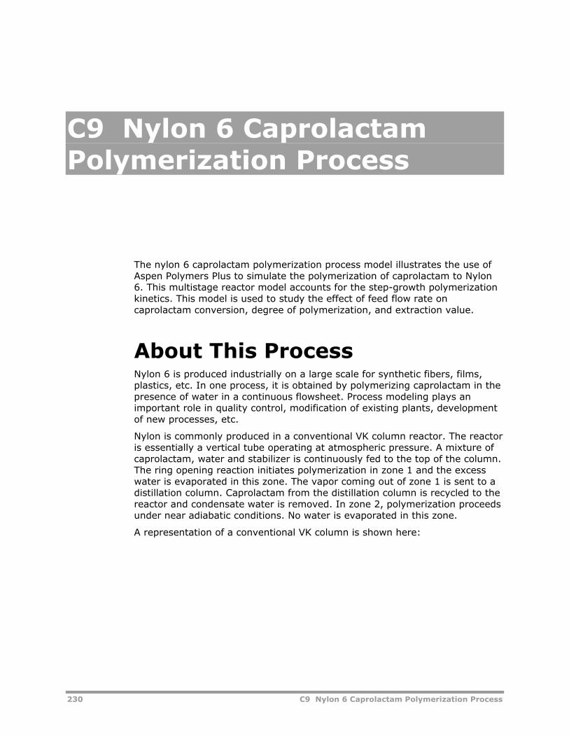
230 C9 Nylon 6 Caprolactam Polymerization Process
C9 Nylon 6 Caprolactam Polymerization Process
The nylon 6 caprolactam polymerization process model illustrates the use of Aspen Polymers Plus to simulate the polymerization of caprolactam to Nylon 6. This multistage reactor model accounts for the step-growth polymerization kinetics. This model is used to study the effect of feed flow rate on caprolactam conversion, degree of polymerization, and extraction value.
About This Process Nylon 6 is produced industrially on a large scale for synthetic fibers, films, plastics, etc. In one process, it is obtained by polymerizing caprolactam in the presence of water in a continuous flowsheet. Process modeling plays an important role in quality control, modification of existing plants, development of new processes, etc.
Nylon is commonly produced in a conventional VK column reactor. The reactor is essentially a vertical tube operating at atmospheric pressure. A mixture of caprolactam, water and stabilizer is continuously fed to the top of the column. The ring opening reaction initiates polymerization in zone 1 and the excess water is evaporated in this zone. The vapor coming out of zone 1 is sent to a distillation column. Caprolactam from the distillation column is recycled to the reactor and condensate water is removed. In zone 2, polymerization proceeds under near adiabatic conditions. No water is evaporated in this zone.
A representation of a conventional VK column is shown here:
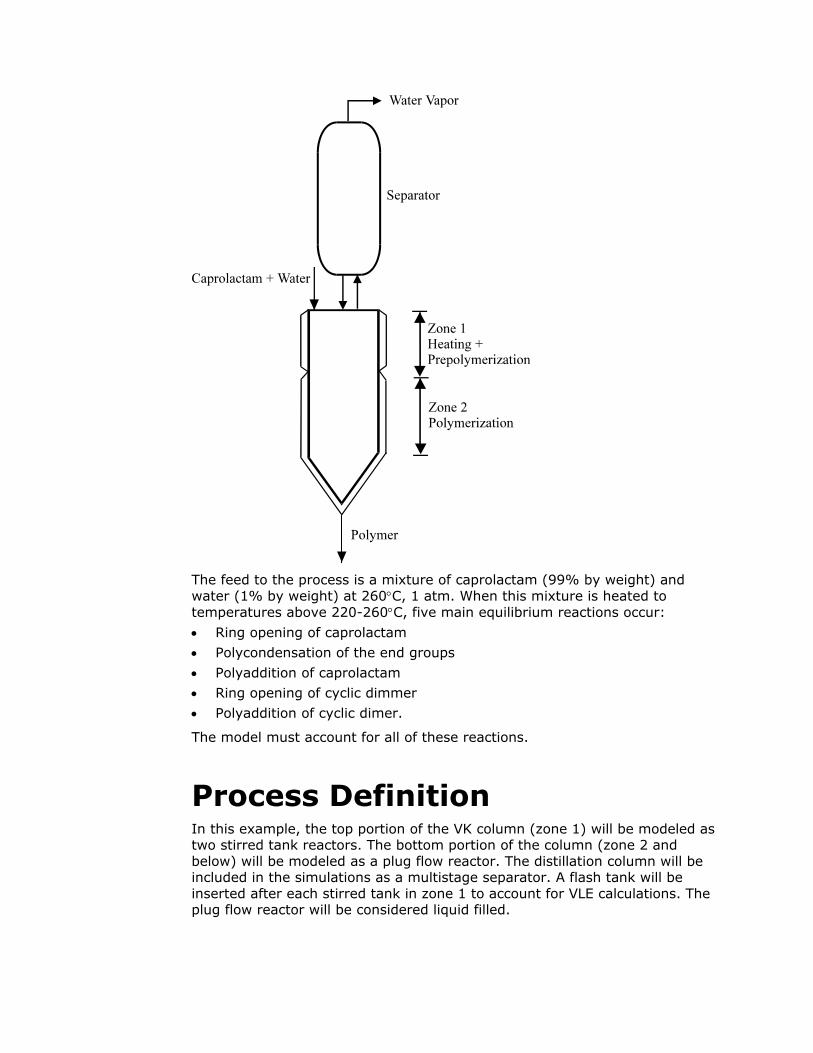
The feed to the process is a mixture of caprolactam (99% by weight) and water (1% by weight) at 260°C, 1 atm. When this mixture is heated to temperatures above 220-260°C, five main equilibrium reactions occur:
• Ring opening of caprolactam
• Polycondensation of the end groups
• Polyaddition of caprolactam
• Ring opening of cyclic dimmer
• Polyaddition of cyclic dimer.
The model must account for all of these reactions.
Process Definition In this example, the top portion of the VK column (zone 1) will be modeled as two stirred tank reactors. The bottom portion of the column (zone 2 and below) will be modeled as a plug flow reactor. The distillation column will be included in the simulations as a multistage separator. A flash tank will be inserted after each stirred tank in zone 1 to account for VLE calculations. The plug flow reactor will be considered liquid filled.
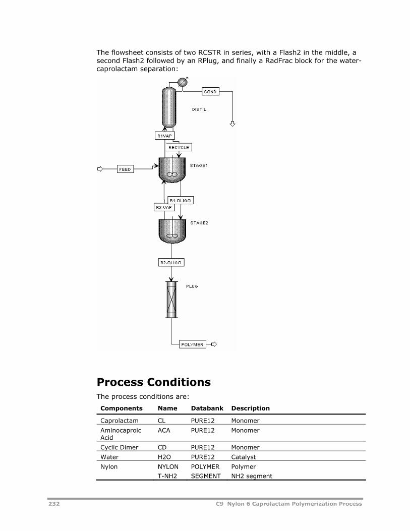
232 C9 Nylon 6 Caprolactam Polymerization Process
The flowsheet consists of two RCSTR in series, with a Flash2 in the middle, a second Flash2 followed by an RPlug, and finally a RadFrac block for the water-caprolactam separation:
Process Conditions The process conditions are:
Components Name Databank Description
Caprolactam CL PURE12 Monomer
Aminocaproic Acid
ACA PURE12 Monomer
Cyclic Dimer CD PURE12 Monomer
Water H2O PURE12 Catalyst
Nylon NYLON
T-NH2
POLYMER
SEGMENT
Polymer
NH2 segment
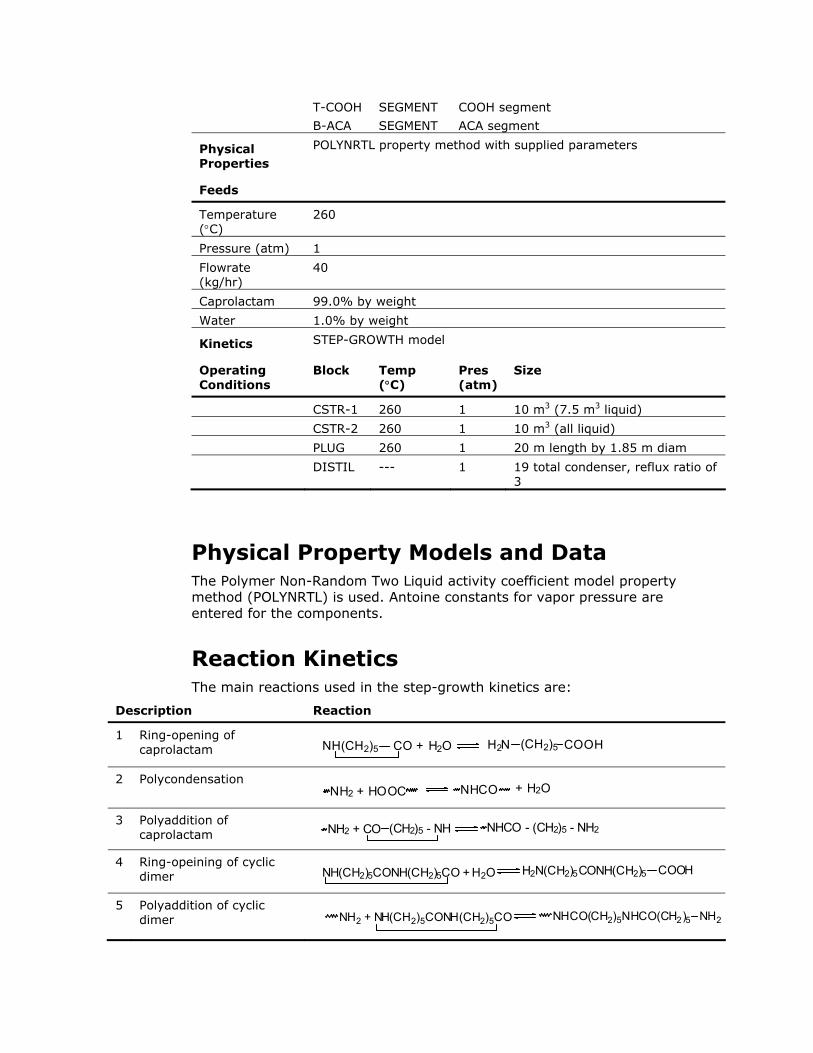
T-COOH
B-ACA
SEGMENT
SEGMENT
COOH segment
ACA segment
Physical Properties
POLYNRTL property method with supplied parameters
Feeds
Temperature (°C)
260
Pressure (atm) 1
Flowrate (kg/hr)
40
Caprolactam 99.0% by weight
Water 1.0% by weight
Kinetics STEP-GROWTH model
Operating Conditions
Block Temp (°C)
Pres (atm)
Size
CSTR-1 260 1 10 m3 (7.5 m3 liquid)
CSTR-2 260 1 10 m3 (all liquid)
PLUG 260 1 20 m length by 1.85 m diam
DISTIL --- 1 19 total condenser, reflux ratio of 3
Physical Property Models and Data The Polymer Non-Random Two Liquid activity coefficient model property method (POLYNRTL) is used. Antoine constants for vapor pressure are entered for the components.
Reaction Kinetics The main reactions used in the step-growth kinetics are:
Description Reaction
1 Ring-opening of caprolactam H2N (CH2)5 COOHNH(CH2)5 CO + H2O
2 Polycondensation
NH2 + HOOC NHCO + H2O
3 Polyaddition of caprolactam NH2 + CO (CH2)5 - NH NHCO - (CH2)5 - NH2
4 Ring-opeining of cyclic
dimer NH(CH2)5CONH(CH2)5CO + H2O H2N(CH2)5CONH(CH2)5 COOH
5 Polyaddition of cyclic dimer NH2 + NH(CH2)5CONH(CH2)5CO NHCO(CH2)5NHCO(CH2)5 NH2
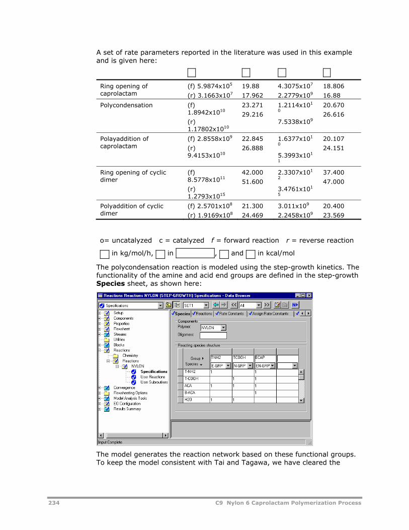
234 C9 Nylon 6 Caprolactam Polymerization Process
A set of rate parameters reported in the literature was used in this example and is given here:
Ring opening of caprolactam
(f) 5.9874x10⁵
(r) 3.1663x10⁷
19.88
17.962
4.3075x10⁷
2.2779x10⁹
18.806
16.88
Polycondensation (f) 1.8942x10¹⁰
(r) 1.17802x10¹⁰
23.271
29.216
1.2114x101
0
7.5338x10⁹
20.670
26.616
Polayaddition of caprolactam
(f) 2.8558x10⁹
(r) 9.4153x10¹⁰
22.845
26.888
1.6377x101
0
5.3993x101
1
20.107
24.151
Ring opening of cyclic dimer
(f) 8.5778x10¹¹
(r) 1.2793x10¹⁵
42.000
51.600
2.3307x101
2
3.4761x101
5
37.400
47.000
Polyaddition of cyclic dimer
(f) 2.5701x10⁸
(r) 1.9169x10⁸
21.300
24.469
3.011x10⁹
2.2458x10⁹
20.400
23.569
o= uncatalyzed c = catalyzed f = forward reaction r = reverse reaction
in kg/mol/h, in , and in kcal/mol
The polycondensation reaction is modeled using the step-growth kinetics. The functionality of the amine and acid end groups are defined in the step-growth Species sheet, as shown here:
The model generates the reaction network based on these functional groups. To keep the model consistent with Tai and Tagawa, we have cleared the
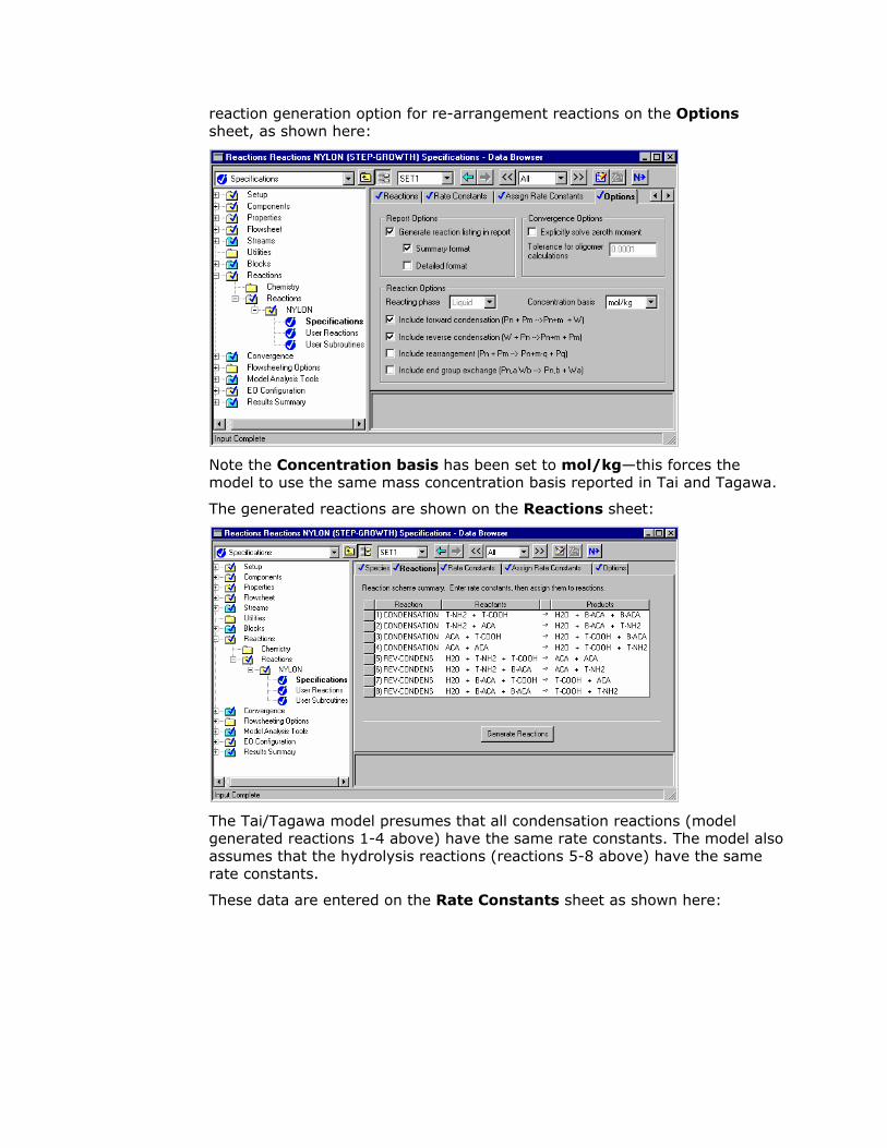
reaction generation option for re-arrangement reactions on the Options sheet, as shown here:
Note the Concentration basis has been set to mol/kg—this forces the model to use the same mass concentration basis reported in Tai and Tagawa.
The generated reactions are shown on the Reactions sheet:
The Tai/Tagawa model presumes that all condensation reactions (model generated reactions 1-4 above) have the same rate constants. The model also assumes that the hydrolysis reactions (reactions 5-8 above) have the same rate constants.
These data are entered on the Rate Constants sheet as shown here:
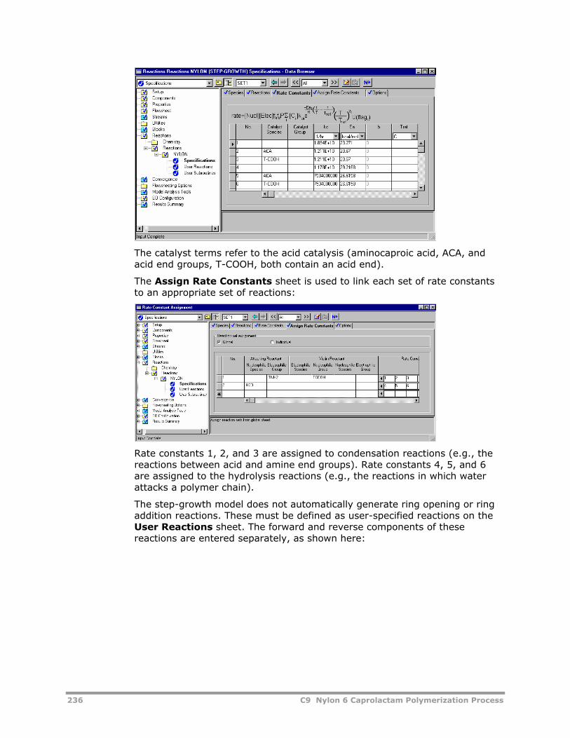
236 C9 Nylon 6 Caprolactam Polymerization Process
The catalyst terms refer to the acid catalysis (aminocaproic acid, ACA, and acid end groups, T-COOH, both contain an acid end).
The Assign Rate Constants sheet is used to link each set of rate constants to an appropriate set of reactions:
Rate constants 1, 2, and 3 are assigned to condensation reactions (e.g., the reactions between acid and amine end groups). Rate constants 4, 5, and 6 are assigned to the hydrolysis reactions (e.g., the reactions in which water attacks a polymer chain).
The step-growth model does not automatically generate ring opening or ring addition reactions. These must be defined as user-specified reactions on the User Reactions sheet. The forward and reverse components of these reactions are entered separately, as shown here:
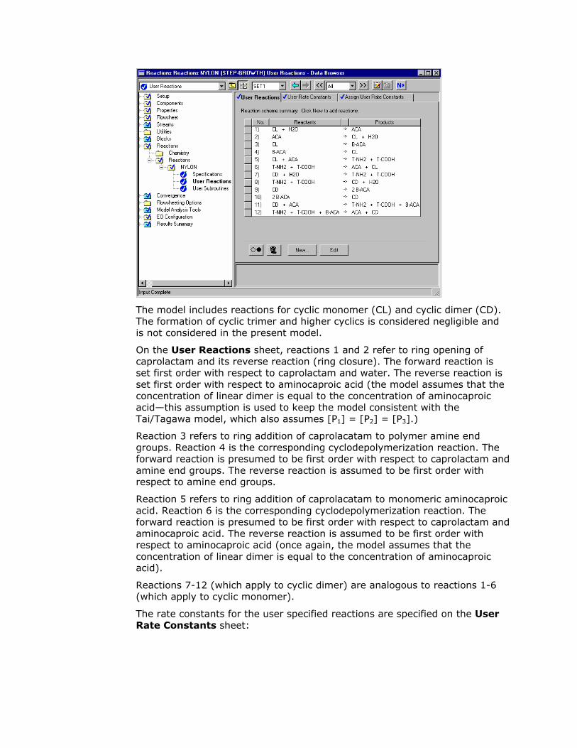
The model includes reactions for cyclic monomer (CL) and cyclic dimer (CD). The formation of cyclic trimer and higher cyclics is considered negligible and is not considered in the present model.
On the User Reactions sheet, reactions 1 and 2 refer to ring opening of caprolactam and its reverse reaction (ring closure). The forward reaction is set first order with respect to caprolactam and water. The reverse reaction is set first order with respect to aminocaproic acid (the model assumes that the concentration of linear dimer is equal to the concentration of aminocaproic acid—this assumption is used to keep the model consistent with the Tai/Tagawa model, which also assumes [P1] = [P2] = [P3].)
Reaction 3 refers to ring addition of caprolacatam to polymer amine end groups. Reaction 4 is the corresponding cyclodepolymerization reaction. The forward reaction is presumed to be first order with respect to caprolactam and amine end groups. The reverse reaction is assumed to be first order with respect to amine end groups.
Reaction 5 refers to ring addition of caprolacatam to monomeric aminocaproic acid. Reaction 6 is the corresponding cyclodepolymerization reaction. The forward reaction is presumed to be first order with respect to caprolactam and aminocaproic acid. The reverse reaction is assumed to be first order with respect to aminocaproic acid (once again, the model assumes that the concentration of linear dimer is equal to the concentration of aminocaproic acid).
Reactions 7-12 (which apply to cyclic dimer) are analogous to reactions 1-6 (which apply to cyclic monomer).
The rate constants for the user specified reactions are specified on the User Rate Constants sheet:
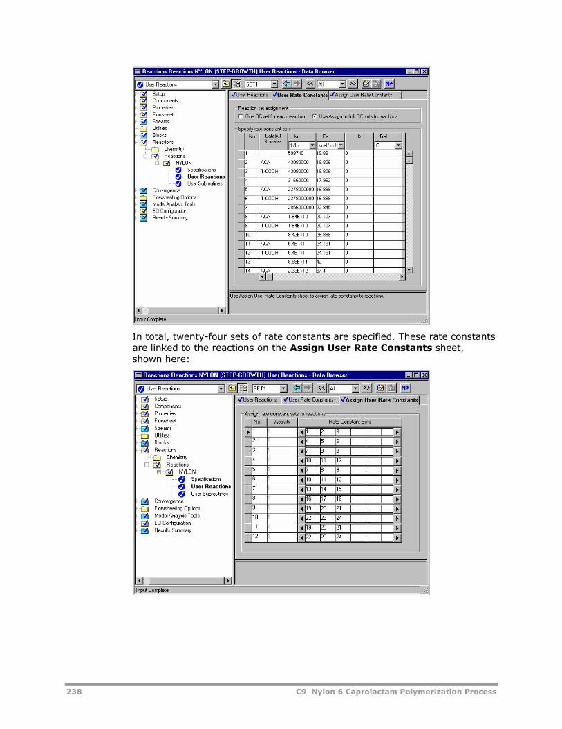
238 C9 Nylon 6 Caprolactam Polymerization Process
In total, twenty-four sets of rate constants are specified. These rate constants are linked to the reactions on the Assign User Rate Constants sheet, shown here:
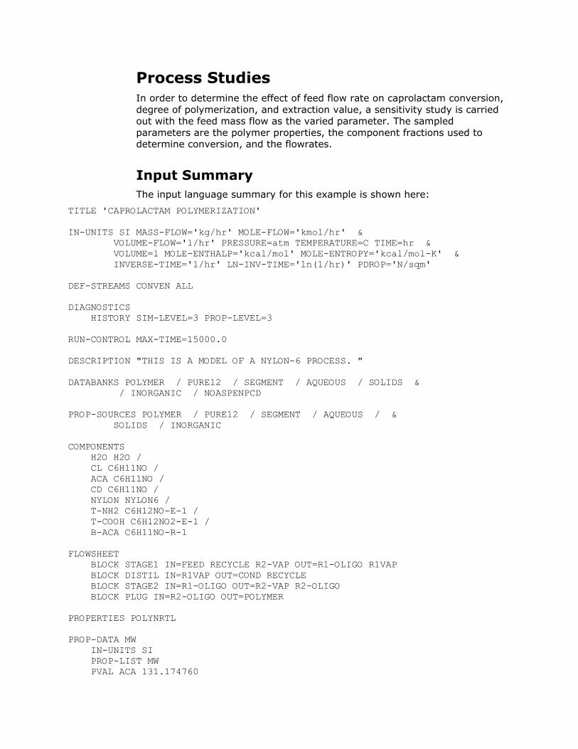
Process Studies In order to determine the effect of feed flow rate on caprolactam conversion, degree of polymerization, and extraction value, a sensitivity study is carried out with the feed mass flow as the varied parameter. The sampled parameters are the polymer properties, the component fractions used to determine conversion, and the flowrates.
Input Summary The input language summary for this example is shown here:
TITLE 'CAPROLACTAM POLYMERIZATION' IN-UNITS SI MASS-FLOW='kg/hr' MOLE-FLOW='kmol/hr' & VOLUME-FLOW='l/hr' PRESSURE=atm TEMPERATURE=C TIME=hr & VOLUME=l MOLE-ENTHALP='kcal/mol' MOLE-ENTROPY='kcal/mol-K' & INVERSE-TIME='1/hr' LN-INV-TIME='ln(1/hr)' PDROP='N/sqm' DEF-STREAMS CONVEN ALL DIAGNOSTICS HISTORY SIM-LEVEL=3 PROP-LEVEL=3 RUN-CONTROL MAX-TIME=15000.0 DESCRIPTION "THIS IS A MODEL OF A NYLON-6 PROCESS. " DATABANKS POLYMER / PURE12 / SEGMENT / AQUEOUS / SOLIDS & / INORGANIC / NOASPENPCD PROP-SOURCES POLYMER / PURE12 / SEGMENT / AQUEOUS / & SOLIDS / INORGANIC COMPONENTS H2O H2O / CL C6H11NO / ACA C6H11NO / CD C6H11NO / NYLON NYLON6 / T-NH2 C6H12NO-E-1 / T-COOH C6H12NO2-E-1 / B-ACA C6H11NO-R-1 FLOWSHEET BLOCK STAGE1 IN=FEED RECYCLE R2-VAP OUT=R1-OLIGO R1VAP BLOCK DISTIL IN=R1VAP OUT=COND RECYCLE BLOCK STAGE2 IN=R1-OLIGO OUT=R2-VAP R2-OLIGO BLOCK PLUG IN=R2-OLIGO OUT=POLYMER PROPERTIES POLYNRTL PROP-DATA MW IN-UNITS SI PROP-LIST MW PVAL ACA 131.174760
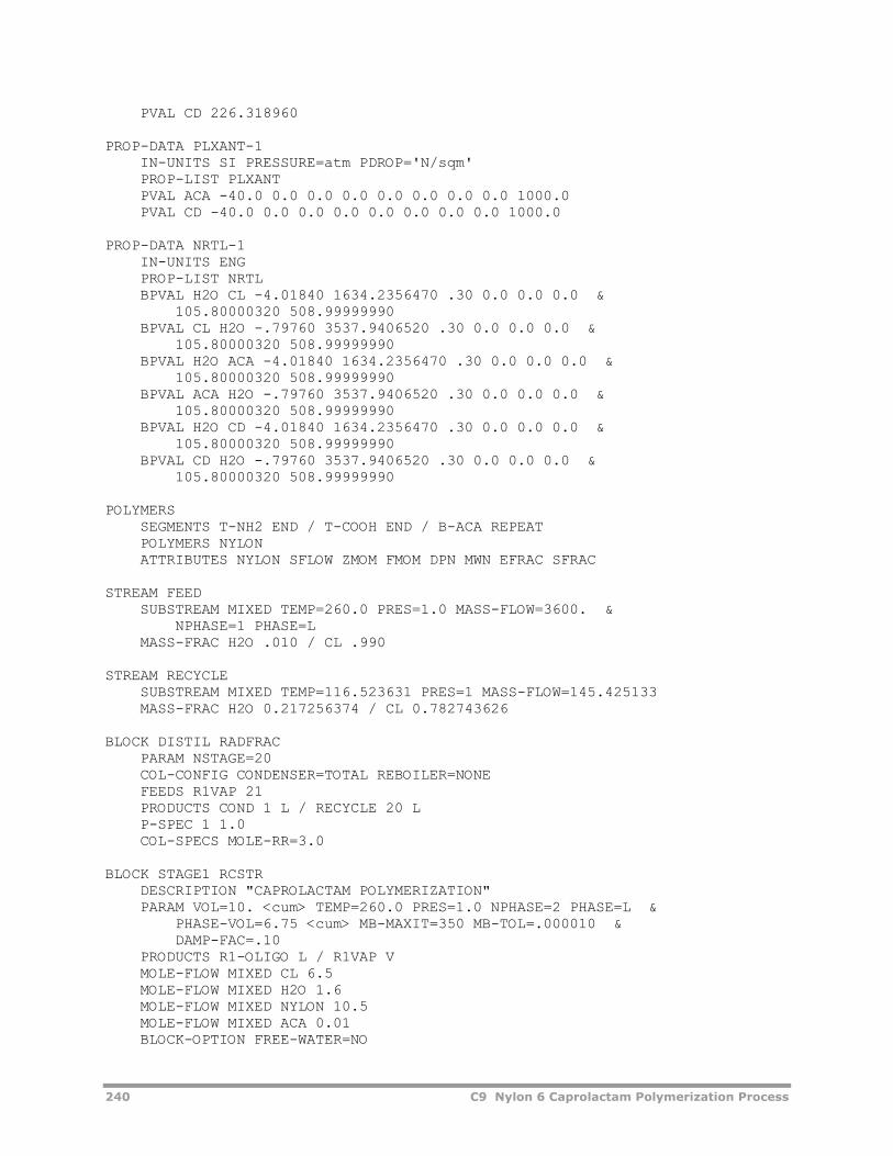
240 C9 Nylon 6 Caprolactam Polymerization Process
PVAL CD 226.318960 PROP-DATA PLXANT-1 IN-UNITS SI PRESSURE=atm PDROP='N/sqm' PROP-LIST PLXANT PVAL ACA -40.0 0.0 0.0 0.0 0.0 0.0 0.0 0.0 1000.0 PVAL CD -40.0 0.0 0.0 0.0 0.0 0.0 0.0 0.0 1000.0 PROP-DATA NRTL-1 IN-UNITS ENG PROP-LIST NRTL BPVAL H2O CL -4.01840 1634.2356470 .30 0.0 0.0 0.0 & 105.80000320 508.99999990 BPVAL CL H2O -.79760 3537.9406520 .30 0.0 0.0 0.0 & 105.80000320 508.99999990 BPVAL H2O ACA -4.01840 1634.2356470 .30 0.0 0.0 0.0 & 105.80000320 508.99999990 BPVAL ACA H2O -.79760 3537.9406520 .30 0.0 0.0 0.0 & 105.80000320 508.99999990 BPVAL H2O CD -4.01840 1634.2356470 .30 0.0 0.0 0.0 & 105.80000320 508.99999990 BPVAL CD H2O -.79760 3537.9406520 .30 0.0 0.0 0.0 & 105.80000320 508.99999990 POLYMERS SEGMENTS T-NH2 END / T-COOH END / B-ACA REPEAT POLYMERS NYLON ATTRIBUTES NYLON SFLOW ZMOM FMOM DPN MWN EFRAC SFRAC STREAM FEED SUBSTREAM MIXED TEMP=260.0 PRES=1.0 MASS-FLOW=3600. & NPHASE=1 PHASE=L MASS-FRAC H2O .010 / CL .990 STREAM RECYCLE SUBSTREAM MIXED TEMP=116.523631 PRES=1 MASS-FLOW=145.425133 MASS-FRAC H2O 0.217256374 / CL 0.782743626 BLOCK DISTIL RADFRAC PARAM NSTAGE=20 COL-CONFIG CONDENSER=TOTAL REBOILER=NONE FEEDS R1VAP 21 PRODUCTS COND 1 L / RECYCLE 20 L P-SPEC 1 1.0 COL-SPECS MOLE-RR=3.0 BLOCK STAGE1 RCSTR DESCRIPTION "CAPROLACTAM POLYMERIZATION" PARAM VOL=10. <cum> TEMP=260.0 PRES=1.0 NPHASE=2 PHASE=L & PHASE-VOL=6.75 <cum> MB-MAXIT=350 MB-TOL=.000010 & DAMP-FAC=.10 PRODUCTS R1-OLIGO L / R1VAP V MOLE-FLOW MIXED CL 6.5 MOLE-FLOW MIXED H2O 1.6 MOLE-FLOW MIXED NYLON 10.5 MOLE-FLOW MIXED ACA 0.01 BLOCK-OPTION FREE-WATER=NO
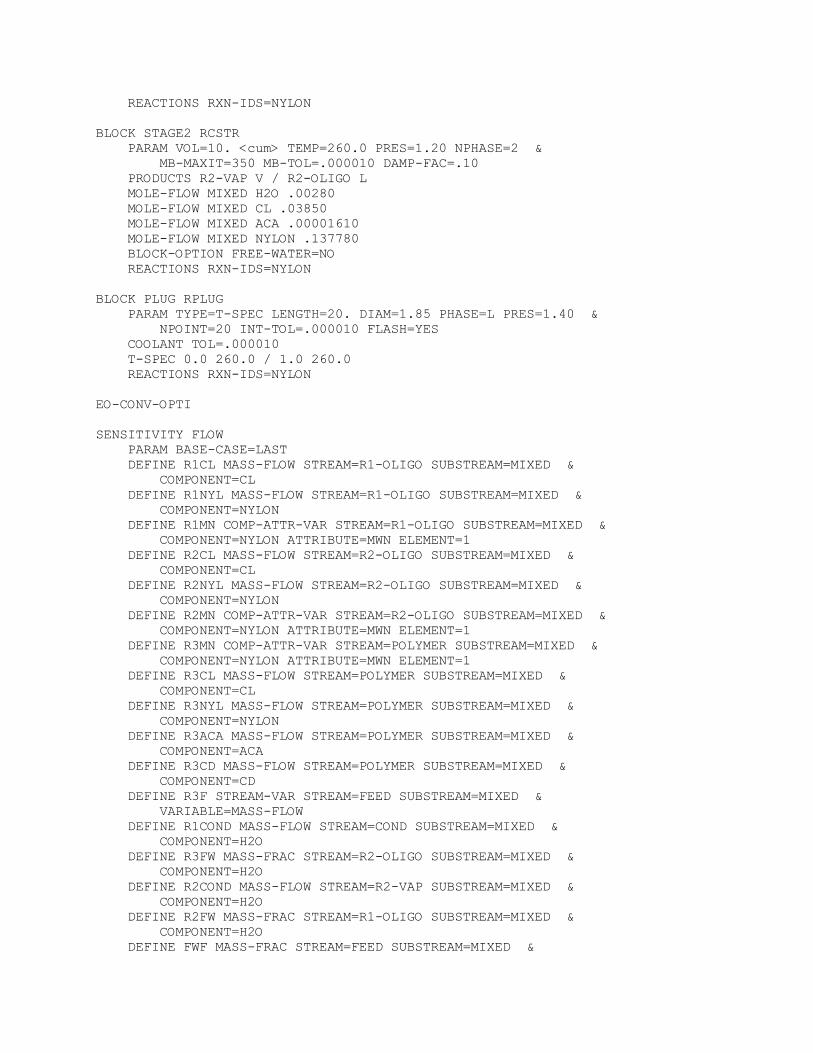
REACTIONS RXN-IDS=NYLON BLOCK STAGE2 RCSTR PARAM VOL=10. <cum> TEMP=260.0 PRES=1.20 NPHASE=2 & MB-MAXIT=350 MB-TOL=.000010 DAMP-FAC=.10 PRODUCTS R2-VAP V / R2-OLIGO L MOLE-FLOW MIXED H2O .00280 MOLE-FLOW MIXED CL .03850 MOLE-FLOW MIXED ACA .00001610 MOLE-FLOW MIXED NYLON .137780 BLOCK-OPTION FREE-WATER=NO REACTIONS RXN-IDS=NYLON BLOCK PLUG RPLUG PARAM TYPE=T-SPEC LENGTH=20. DIAM=1.85 PHASE=L PRES=1.40 & NPOINT=20 INT-TOL=.000010 FLASH=YES COOLANT TOL=.000010 T-SPEC 0.0 260.0 / 1.0 260.0 REACTIONS RXN-IDS=NYLON EO-CONV-OPTI SENSITIVITY FLOW PARAM BASE-CASE=LAST DEFINE R1CL MASS-FLOW STREAM=R1-OLIGO SUBSTREAM=MIXED & COMPONENT=CL DEFINE R1NYL MASS-FLOW STREAM=R1-OLIGO SUBSTREAM=MIXED & COMPONENT=NYLON DEFINE R1MN COMP-ATTR-VAR STREAM=R1-OLIGO SUBSTREAM=MIXED & COMPONENT=NYLON ATTRIBUTE=MWN ELEMENT=1 DEFINE R2CL MASS-FLOW STREAM=R2-OLIGO SUBSTREAM=MIXED & COMPONENT=CL DEFINE R2NYL MASS-FLOW STREAM=R2-OLIGO SUBSTREAM=MIXED & COMPONENT=NYLON DEFINE R2MN COMP-ATTR-VAR STREAM=R2-OLIGO SUBSTREAM=MIXED & COMPONENT=NYLON ATTRIBUTE=MWN ELEMENT=1 DEFINE R3MN COMP-ATTR-VAR STREAM=POLYMER SUBSTREAM=MIXED & COMPONENT=NYLON ATTRIBUTE=MWN ELEMENT=1 DEFINE R3CL MASS-FLOW STREAM=POLYMER SUBSTREAM=MIXED & COMPONENT=CL DEFINE R3NYL MASS-FLOW STREAM=POLYMER SUBSTREAM=MIXED & COMPONENT=NYLON DEFINE R3ACA MASS-FLOW STREAM=POLYMER SUBSTREAM=MIXED & COMPONENT=ACA DEFINE R3CD MASS-FLOW STREAM=POLYMER SUBSTREAM=MIXED & COMPONENT=CD DEFINE R3F STREAM-VAR STREAM=FEED SUBSTREAM=MIXED & VARIABLE=MASS-FLOW DEFINE R1COND MASS-FLOW STREAM=COND SUBSTREAM=MIXED & COMPONENT=H2O DEFINE R3FW MASS-FRAC STREAM=R2-OLIGO SUBSTREAM=MIXED & COMPONENT=H2O DEFINE R2COND MASS-FLOW STREAM=R2-VAP SUBSTREAM=MIXED & COMPONENT=H2O DEFINE R2FW MASS-FRAC STREAM=R1-OLIGO SUBSTREAM=MIXED & COMPONENT=H2O DEFINE FWF MASS-FRAC STREAM=FEED SUBSTREAM=MIXED &
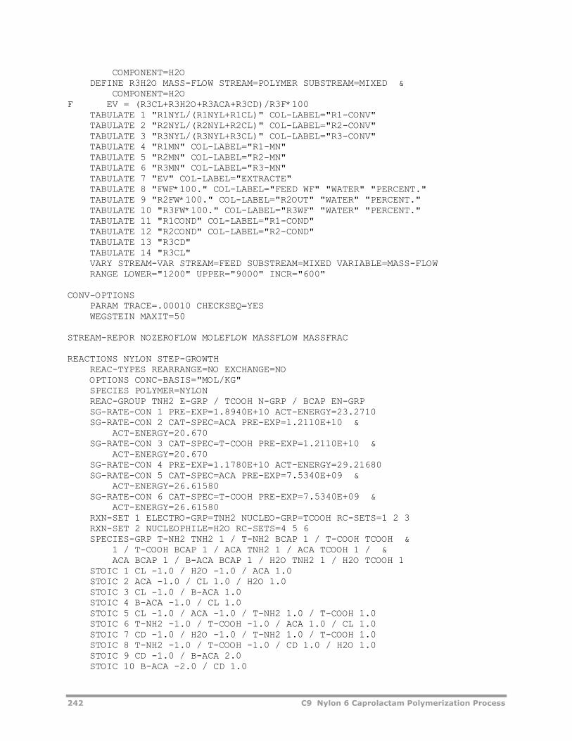
242 C9 Nylon 6 Caprolactam Polymerization Process
COMPONENT=H2O DEFINE R3H2O MASS-FLOW STREAM=POLYMER SUBSTREAM=MIXED & COMPONENT=H2O F EV = (R3CL+R3H2O+R3ACA+R3CD)/R3F*100 TABULATE 1 "R1NYL/(R1NYL+R1CL)" COL-LABEL="R1-CONV" TABULATE 2 "R2NYL/(R2NYL+R2CL)" COL-LABEL="R2-CONV" TABULATE 3 "R3NYL/(R3NYL+R3CL)" COL-LABEL="R3-CONV" TABULATE 4 "R1MN" COL-LABEL="R1-MN" TABULATE 5 "R2MN" COL-LABEL="R2-MN" TABULATE 6 "R3MN" COL-LABEL="R3-MN" TABULATE 7 "EV" COL-LABEL="EXTRACTE" TABULATE 8 "FWF*100." COL-LABEL="FEED WF" "WATER" "PERCENT." TABULATE 9 "R2FW*100." COL-LABEL="R2OUT" "WATER" "PERCENT." TABULATE 10 "R3FW*100." COL-LABEL="R3WF" "WATER" "PERCENT." TABULATE 11 "R1COND" COL-LABEL="R1-COND" TABULATE 12 "R2COND" COL-LABEL="R2-COND" TABULATE 13 "R3CD" TABULATE 14 "R3CL" VARY STREAM-VAR STREAM=FEED SUBSTREAM=MIXED VARIABLE=MASS-FLOW RANGE LOWER="1200" UPPER="9000" INCR="600" CONV-OPTIONS PARAM TRACE=.00010 CHECKSEQ=YES WEGSTEIN MAXIT=50 STREAM-REPOR NOZEROFLOW MOLEFLOW MASSFLOW MASSFRAC REACTIONS NYLON STEP-GROWTH REAC-TYPES REARRANGE=NO EXCHANGE=NO OPTIONS CONC-BASIS="MOL/KG" SPECIES POLYMER=NYLON REAC-GROUP TNH2 E-GRP / TCOOH N-GRP / BCAP EN-GRP SG-RATE-CON 1 PRE-EXP=1.8940E+10 ACT-ENERGY=23.2710 SG-RATE-CON 2 CAT-SPEC=ACA PRE-EXP=1.2110E+10 & ACT-ENERGY=20.670 SG-RATE-CON 3 CAT-SPEC=T-COOH PRE-EXP=1.2110E+10 & ACT-ENERGY=20.670 SG-RATE-CON 4 PRE-EXP=1.1780E+10 ACT-ENERGY=29.21680 SG-RATE-CON 5 CAT-SPEC=ACA PRE-EXP=7.5340E+09 & ACT-ENERGY=26.61580 SG-RATE-CON 6 CAT-SPEC=T-COOH PRE-EXP=7.5340E+09 & ACT-ENERGY=26.61580 RXN-SET 1 ELECTRO-GRP=TNH2 NUCLEO-GRP=TCOOH RC-SETS=1 2 3 RXN-SET 2 NUCLEOPHILE=H2O RC-SETS=4 5 6 SPECIES-GRP T-NH2 TNH2 1 / T-NH2 BCAP 1 / T-COOH TCOOH & 1 / T-COOH BCAP 1 / ACA TNH2 1 / ACA TCOOH 1 / & ACA BCAP 1 / B-ACA BCAP 1 / H2O TNH2 1 / H2O TCOOH 1 STOIC 1 CL -1.0 / H2O -1.0 / ACA 1.0 STOIC 2 ACA -1.0 / CL 1.0 / H2O 1.0 STOIC 3 CL -1.0 / B-ACA 1.0 STOIC 4 B-ACA -1.0 / CL 1.0 STOIC 5 CL -1.0 / ACA -1.0 / T-NH2 1.0 / T-COOH 1.0 STOIC 6 T-NH2 -1.0 / T-COOH -1.0 / ACA 1.0 / CL 1.0 STOIC 7 CD -1.0 / H2O -1.0 / T-NH2 1.0 / T-COOH 1.0 STOIC 8 T-NH2 -1.0 / T-COOH -1.0 / CD 1.0 / H2O 1.0 STOIC 9 CD -1.0 / B-ACA 2.0 STOIC 10 B-ACA -2.0 / CD 1.0
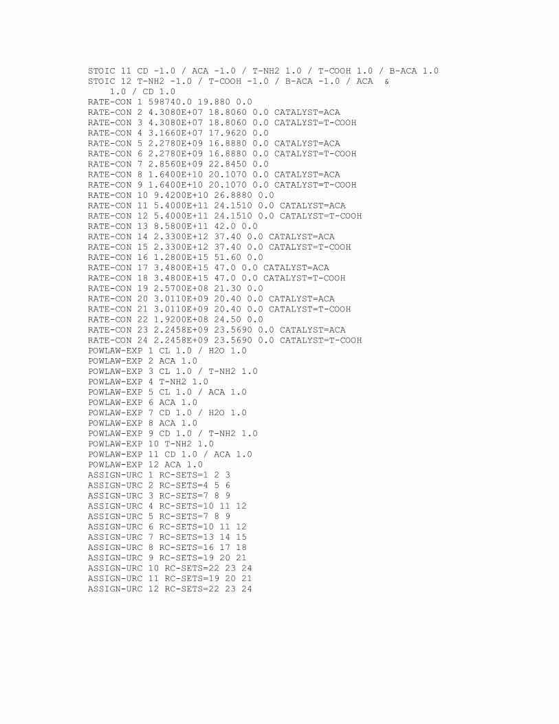
STOIC 11 CD -1.0 / ACA -1.0 / T-NH2 1.0 / T-COOH 1.0 / B-ACA 1.0 STOIC 12 T-NH2 -1.0 / T-COOH -1.0 / B-ACA -1.0 / ACA & 1.0 / CD 1.0 RATE-CON 1 598740.0 19.880 0.0 RATE-CON 2 4.3080E+07 18.8060 0.0 CATALYST=ACA RATE-CON 3 4.3080E+07 18.8060 0.0 CATALYST=T-COOH RATE-CON 4 3.1660E+07 17.9620 0.0 RATE-CON 5 2.2780E+09 16.8880 0.0 CATALYST=ACA RATE-CON 6 2.2780E+09 16.8880 0.0 CATALYST=T-COOH RATE-CON 7 2.8560E+09 22.8450 0.0 RATE-CON 8 1.6400E+10 20.1070 0.0 CATALYST=ACA RATE-CON 9 1.6400E+10 20.1070 0.0 CATALYST=T-COOH RATE-CON 10 9.4200E+10 26.8880 0.0 RATE-CON 11 5.4000E+11 24.1510 0.0 CATALYST=ACA RATE-CON 12 5.4000E+11 24.1510 0.0 CATALYST=T-COOH RATE-CON 13 8.5800E+11 42.0 0.0 RATE-CON 14 2.3300E+12 37.40 0.0 CATALYST=ACA RATE-CON 15 2.3300E+12 37.40 0.0 CATALYST=T-COOH RATE-CON 16 1.2800E+15 51.60 0.0 RATE-CON 17 3.4800E+15 47.0 0.0 CATALYST=ACA RATE-CON 18 3.4800E+15 47.0 0.0 CATALYST=T-COOH RATE-CON 19 2.5700E+08 21.30 0.0 RATE-CON 20 3.0110E+09 20.40 0.0 CATALYST=ACA RATE-CON 21 3.0110E+09 20.40 0.0 CATALYST=T-COOH RATE-CON 22 1.9200E+08 24.50 0.0 RATE-CON 23 2.2458E+09 23.5690 0.0 CATALYST=ACA RATE-CON 24 2.2458E+09 23.5690 0.0 CATALYST=T-COOH POWLAW-EXP 1 CL 1.0 / H2O 1.0 POWLAW-EXP 2 ACA 1.0 POWLAW-EXP 3 CL 1.0 / T-NH2 1.0 POWLAW-EXP 4 T-NH2 1.0 POWLAW-EXP 5 CL 1.0 / ACA 1.0 POWLAW-EXP 6 ACA 1.0 POWLAW-EXP 7 CD 1.0 / H2O 1.0 POWLAW-EXP 8 ACA 1.0 POWLAW-EXP 9 CD 1.0 / T-NH2 1.0 POWLAW-EXP 10 T-NH2 1.0 POWLAW-EXP 11 CD 1.0 / ACA 1.0 POWLAW-EXP 12 ACA 1.0 ASSIGN-URC 1 RC-SETS=1 2 3 ASSIGN-URC 2 RC-SETS=4 5 6 ASSIGN-URC 3 RC-SETS=7 8 9 ASSIGN-URC 4 RC-SETS=10 11 12 ASSIGN-URC 5 RC-SETS=7 8 9 ASSIGN-URC 6 RC-SETS=10 11 12 ASSIGN-URC 7 RC-SETS=13 14 15 ASSIGN-URC 8 RC-SETS=16 17 18 ASSIGN-URC 9 RC-SETS=19 20 21 ASSIGN-URC 10 RC-SETS=22 23 24 ASSIGN-URC 11 RC-SETS=19 20 21 ASSIGN-URC 12 RC-SETS=22 23 24
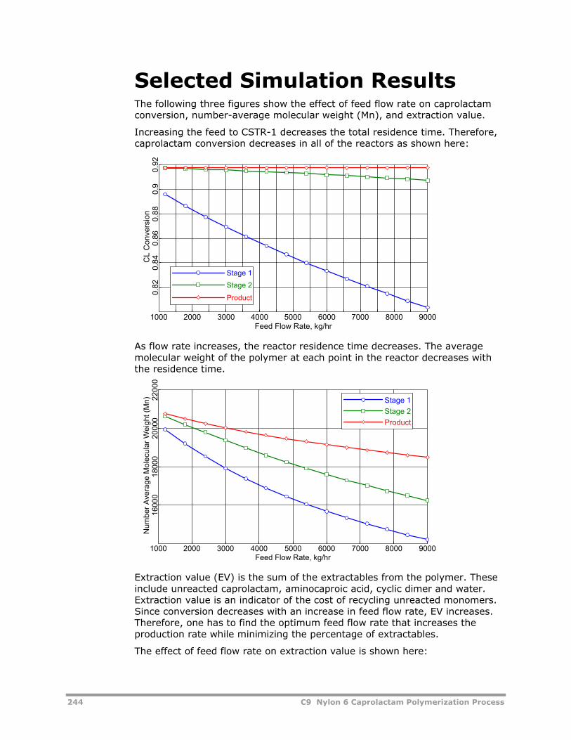
244 C9 Nylon 6 Caprolactam Polymerization Process
Selected Simulation Results The following three figures show the effect of feed flow rate on caprolactam conversion, number-average molecular weight (Mn), and extraction value.
Increasing the feed to CSTR-1 decreases the total residence time. Therefore, caprolactam conversion decreases in all of the reactors as shown here:
Feed Flow Rate, kg/hr
CL
Con
vers
ion
1000 2000 3000 4000 5000 6000 7000 8000 9000
0.82
0.84
0.86
0.88
0.9
0.92
Stage 1Stage 2
Product
As flow rate increases, the reactor residence time decreases. The average molecular weight of the polymer at each point in the reactor decreases with the residence time.
Feed Flow Rate, kg/hr
Num
ber A
vera
ge M
olec
ular
Wei
ght (
Mn)
1000 2000 3000 4000 5000 6000 7000 8000 9000
1600
018
000
2000
022
000
Stage 1Stage 2Product
Extraction value (EV) is the sum of the extractables from the polymer. These include unreacted caprolactam, aminocaproic acid, cyclic dimer and water. Extraction value is an indicator of the cost of recycling unreacted monomers. Since conversion decreases with an increase in feed flow rate, EV increases. Therefore, one has to find the optimum feed flow rate that increases the production rate while minimizing the percentage of extractables.
The effect of feed flow rate on extraction value is shown here:
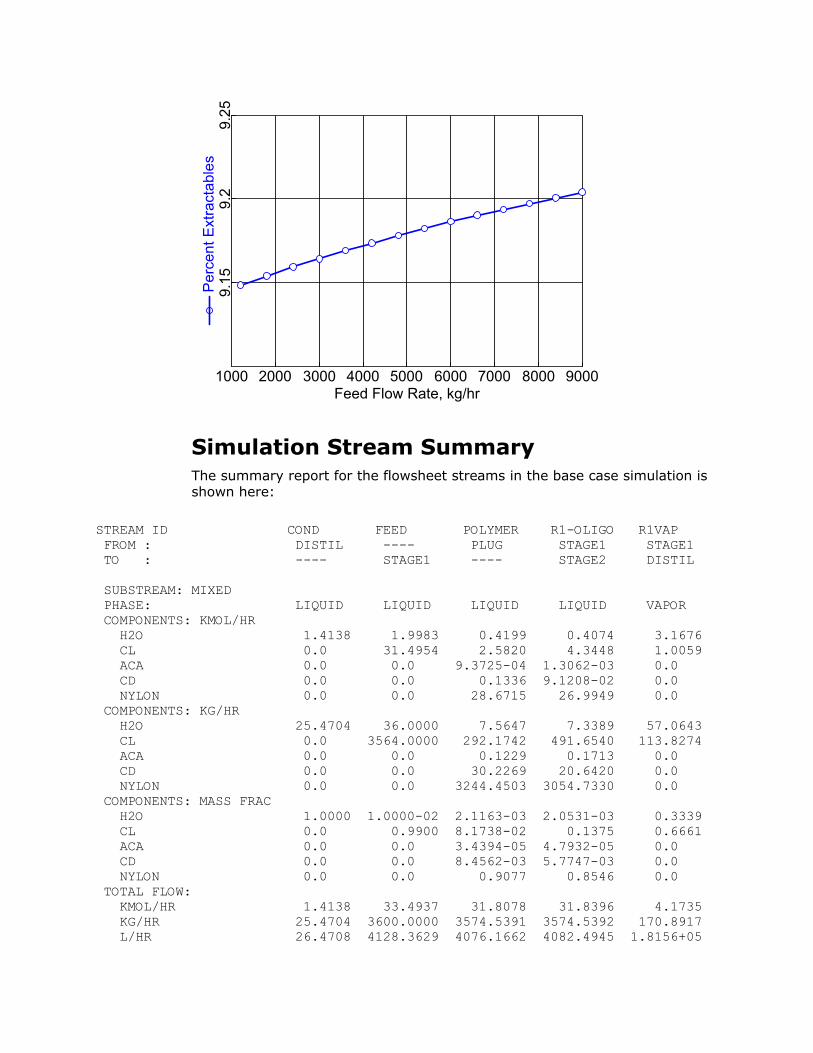
Feed Flow Rate, kg/hr
Per
cent
Ext
ract
able
s
1000 2000 3000 4000 5000 6000 7000 8000 9000
9.15
9.2
9.25
Simulation Stream Summary The summary report for the flowsheet streams in the base case simulation is shown here:
STREAM ID COND FEED POLYMER R1-OLIGO R1VAP FROM : DISTIL ---- PLUG STAGE1 STAGE1 TO : ---- STAGE1 ---- STAGE2 DISTIL SUBSTREAM: MIXED PHASE: LIQUID LIQUID LIQUID LIQUID VAPOR COMPONENTS: KMOL/HR H2O 1.4138 1.9983 0.4199 0.4074 3.1676 CL 0.0 31.4954 2.5820 4.3448 1.0059 ACA 0.0 0.0 9.3725-04 1.3062-03 0.0 CD 0.0 0.0 0.1336 9.1208-02 0.0 NYLON 0.0 0.0 28.6715 26.9949 0.0 COMPONENTS: KG/HR H2O 25.4704 36.0000 7.5647 7.3389 57.0643 CL 0.0 3564.0000 292.1742 491.6540 113.8274 ACA 0.0 0.0 0.1229 0.1713 0.0 CD 0.0 0.0 30.2269 20.6420 0.0 NYLON 0.0 0.0 3244.4503 3054.7330 0.0 COMPONENTS: MASS FRAC H2O 1.0000 1.0000-02 2.1163-03 2.0531-03 0.3339 CL 0.0 0.9900 8.1738-02 0.1375 0.6661 ACA 0.0 0.0 3.4394-05 4.7932-05 0.0 CD 0.0 0.0 8.4562-03 5.7747-03 0.0 NYLON 0.0 0.0 0.9077 0.8546 0.0 TOTAL FLOW: KMOL/HR 1.4138 33.4937 31.8078 31.8396 4.1735 KG/HR 25.4704 3600.0000 3574.5391 3574.5392 170.8917 L/HR 26.4708 4128.3629 4076.1662 4082.4945 1.8156+05
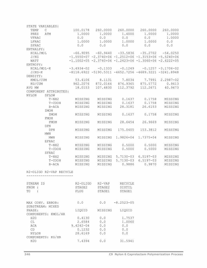
246 C9 Nylon 6 Caprolactam Polymerization Process
STATE VARIABLES: TEMP C 100.0178 260.0000 260.0000 260.0000 260.0000 PRES ATM 1.0000 1.0000 1.4000 1.0000 1.0000 VFRAC 0.0 0.0 0.0 0.0 1.0000 LFRAC 1.0000 1.0000 1.0000 1.0000 0.0 SFRAC 0.0 0.0 0.0 0.0 0.0 ENTHALPY: KCAL/MOL -66.9095 -60.9440 -33.5836 -35.2702 -54.0250 J/KG -1.5550+07 -2.3740+06 -1.2512+06 -1.3153+06 -5.5240+06 WATT -1.1002+05 -2.3740+06 -1.2423+06 -1.3060+06 -2.6222+05 ENTROPY: KCAL/MOL-K -3.4934-02 -0.1333 -0.1249 -0.1257 -3.1706-02 J/KG-K -8118.6922 -5190.5311 -4652.7256 -4689.3221 -3241.8948 DENSITY: KMOL/CUM 53.4106 8.1131 7.8034 7.7991 2.2987-02 KG/CUM 962.2076 872.0164 876.9365 875.5772 0.9413 AVG MW 18.0153 107.4830 112.3792 112.2671 40.9473 COMPONENT ATTRIBUTES: NYLON SFLOW T-NH2 MISSING MISSING 0.1637 0.1758 MISSING T-COOH MISSING MISSING 0.1637 0.1758 MISSING B-ACA MISSING MISSING 28.3181 26.6153 MISSING ZMOM ZMOM MISSING MISSING 0.1637 0.1758 MISSING FMOM FMOM MISSING MISSING 28.6454 26.9669 MISSING DPN DPN MISSING MISSING 175.0405 153.3812 MISSING MWN MWN MISSING MISSING 1.9826+04 1.7375+04 MISSING EFRAC T-NH2 MISSING MISSING 0.5000 0.5000 MISSING T-COOH MISSING MISSING 0.5000 0.5000 MISSING SFRAC T-NH2 MISSING MISSING 5.7130-03 6.5197-03 MISSING T-COOH MISSING MISSING 5.7130-03 6.5197-03 MISSING B-ACA MISSING MISSING 0.9886 0.9870 MISSING R2-OLIGO R2-VAP RECYCLE ----------------------- STREAM ID R2-OLIGO R2-VAP RECYCLE FROM : STAGE2 STAGE2 DISTIL TO : PLUG STAGE1 STAGE1 MAX CONV. ERROR: 0.0 0.0 -8.2523-05 SUBSTREAM: MIXED PHASE: LIQUID MISSING LIQUID COMPONENTS: KMOL/HR H2O 0.4130 0.0 1.7537 CL 2.6584 0.0 1.0060 ACA 9.4242-04 0.0 0.0 CD 0.1232 0.0 0.0 NYLON 28.6169 0.0 0.0 COMPONENTS: KG/HR H2O 7.4394 0.0 31.5941
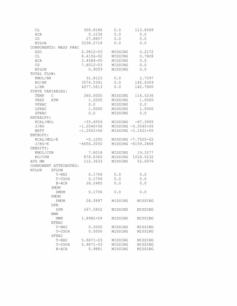
CL 300.8186 0.0 113.8368 ACA 0.1236 0.0 0.0 CD 27.8857 0.0 0.0 NYLON 3238.2718 0.0 0.0 COMPONENTS: MASS FRAC H2O 2.0812-03 MISSING 0.2172 CL 8.4156-02 MISSING 0.7828 ACA 3.4584-05 MISSING 0.0 CD 7.8012-03 MISSING 0.0 NYLON 0.9059 MISSING 0.0 TOTAL FLOW: KMOL/HR 31.8123 0.0 2.7597 KG/HR 3574.5391 0.0 145.4309 L/HR 4077.5613 0.0 142.7860 STATE VARIABLES: TEMP C 260.0000 MISSING 116.5236 PRES ATM 1.2000 MISSING 1.0000 VFRAC 0.0 MISSING 0.0 LFRAC 1.0000 MISSING 1.0000 SFRAC 0.0 MISSING 0.0 ENTHALPY: KCAL/MOL -33.6554 MISSING -67.3955 J/KG -1.2540+06 MISSING -5.3545+06 WATT -1.2452+06 MISSING -2.1631+05 ENTROPY: KCAL/MOL-K -0.1250 MISSING -7.7525-02 J/KG-K -4656.2050 MISSING -6159.2868 DENSITY: KMOL/CUM 7.8018 MISSING 19.3277 KG/CUM 876.6365 MISSING 1018.5232 AVG MW 112.3633 MISSING 52.6976 COMPONENT ATTRIBUTES: NYLON SFLOW T-NH2 0.1706 0.0 0.0 T-COOH 0.1706 0.0 0.0 B-ACA 28.2485 0.0 0.0 ZMOM ZMOM 0.1706 0.0 0.0 FMOM FMOM 28.5897 MISSING MISSING DPN DPN 167.5852 MISSING MISSING MWN MWN 1.8982+04 MISSING MISSING EFRAC T-NH2 0.5000 MISSING MISSING T-COOH 0.5000 MISSING MISSING SFRAC T-NH2 5.9671-03 MISSING MISSING T-COOH 5.9671-03 MISSING MISSING B-ACA 0.9881 MISSING MISSING
248 C9 Nylon 6 Caprolactam Polymerization Process
References Gupta, A. K., & Gandhi, K. S. (1985). Modeling of Backmixing in Continuous Polymerization of Caprolactam in VK Column Reactors. Ind. Eng. Chem. Product Research and Development, 24, p. 327.
Hotyzer P. J., Hoogschagen, J., & Van Krevelen, D. W. (1965). Optimization of Caprolactam Polymerization. Chem. Eng. Sci., 20, p. 247.
Reimschuessel H. K. (1977). Nylon 6: Chemistry and Mechanisms. J. Polymerization Sci.: Macromolecular Reviews, 12, p. 65.
Tai K., Arai, Y., & Tagawa, T. (1982). The Simulation of Hydrolytic Polymerization of Caprolactam in Various Reactors. J. Appl. Polymer Sci., 22, p. 731.
Tai K., & Tagawa, T. (1983). Simulation of Hydrolytic Polymerization of Caprolactam in Various Reactors. A review on recent advances in reaction engineering of polymerization. Industrial & Engineering Chemistry Research, 22, p. 192.
C10 Methyl Methacrylate Polymerization in Ethyl Acetate
The methyl methacrylate polymerization in ethyl acetate model illustrates the use of Aspen Polymers Plus to model a solution polymerization process for methyl methacrylate in ethyl acetate. Among the studies carried out using this model are the effect of initiator concentration and reactor temperature on molecular weight and conversion.
About This Process Polymethyl methacrylate is part of the polyacrylic group of polymers. It is used in the manufacture of lenses or other clear coverings and is also known under the trade names plexiglass, lucite, acrylate, etc.
This methyl methacrylate polymerization is carried out in a free-radical solution process. Solution polymerization is used when both the monomer and the initiator are soluble in the solvent. Typically, solution processes result in low viscosity, provide good mixing, and improve heat transfer limitations, while improving temperature control and reducing gel effect. On the other hand, these processes result in lower reaction rate and in lower polymer molecular weight due to chain transfer to solvents. Furthermore, solvent removal can be costly.
The flowsheet for this process consists of a batch reactor followed by a devolatizer for solvent removal. The reactor feed contains methyl methacrylate dissolved in ethyl acetate, with AIBN as the initiator. The reactor operates under constant temperature and pressure.
Process Definition The batch reactor is modeled using RBatch, and the devolitizer using Flash2:
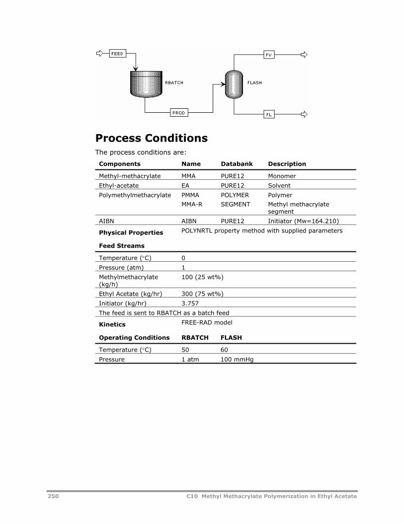
250 C10 Methyl Methacrylate Polymerization in Ethyl Acetate
Process Conditions The process conditions are:
Components Name Databank Description
Methyl-methacrylate MMA PURE12 Monomer
Ethyl-acetate EA PURE12 Solvent
Polymethylmethacrylate PMMA
MMA-R
POLYMER
SEGMENT
Polymer
Methyl methacrylate segment
AIBN AIBN PURE12 Initiator (Mw=164.210)
Physical Properties POLYNRTL property method with supplied parameters
Feed Streams
Temperature (°C) 0
Pressure (atm) 1
Methylmethacrylate (kg/h)
100 (25 wt%)
Ethyl Acetate (kg/hr) 300 (75 wt%)
Initiator (kg/hr) 3.757
The feed is sent to RBATCH as a batch feed
Kinetics FREE-RAD model
Operating Conditions RBATCH FLASH
Temperature (°C) 50 60
Pressure 1 atm 100 mmHg
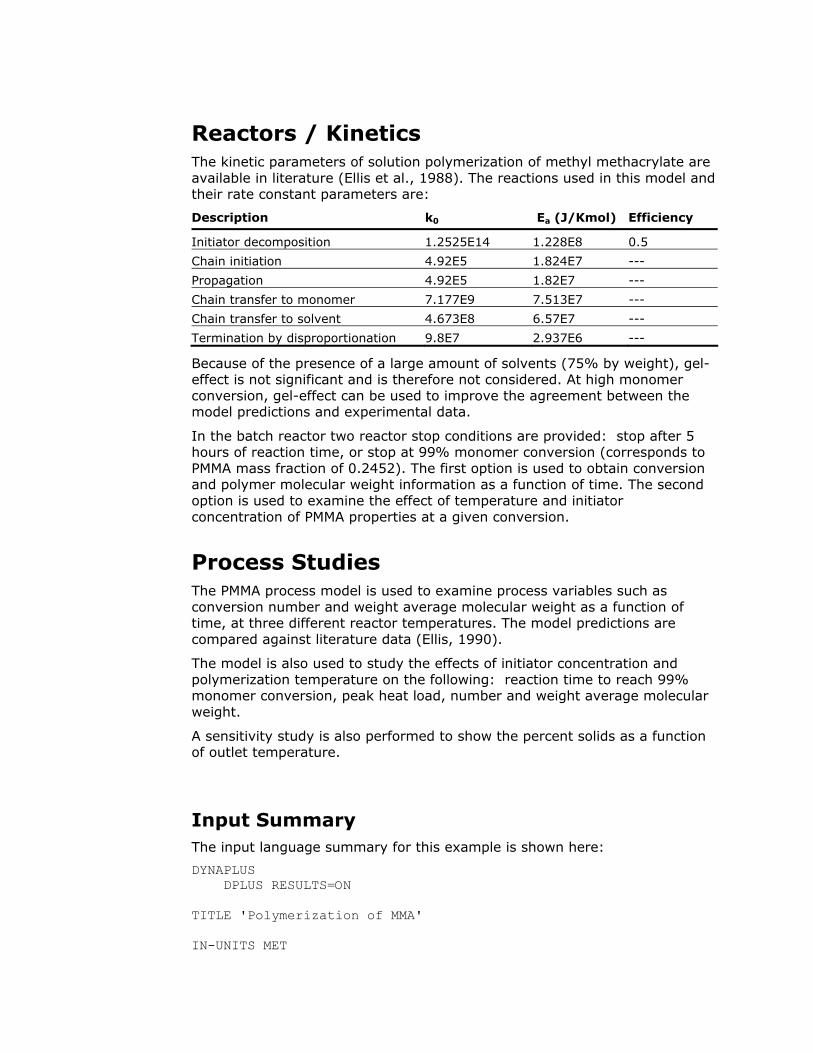
Reactors / Kinetics The kinetic parameters of solution polymerization of methyl methacrylate are available in literature (Ellis et al., 1988). The reactions used in this model and their rate constant parameters are:
Description k0 Ea (J/Kmol) Efficiency
Initiator decomposition 1.2525E14 1.228E8 0.5
Chain initiation 4.92E5 1.824E7 ---
Propagation 4.92E5 1.82E7 ---
Chain transfer to monomer 7.177E9 7.513E7 ---
Chain transfer to solvent 4.673E8 6.57E7 ---
Termination by disproportionation 9.8E7 2.937E6 ---
Because of the presence of a large amount of solvents (75% by weight), gel-effect is not significant and is therefore not considered. At high monomer conversion, gel-effect can be used to improve the agreement between the model predictions and experimental data.
In the batch reactor two reactor stop conditions are provided: stop after 5 hours of reaction time, or stop at 99% monomer conversion (corresponds to PMMA mass fraction of 0.2452). The first option is used to obtain conversion and polymer molecular weight information as a function of time. The second option is used to examine the effect of temperature and initiator concentration of PMMA properties at a given conversion.
Process Studies The PMMA process model is used to examine process variables such as conversion number and weight average molecular weight as a function of time, at three different reactor temperatures. The model predictions are compared against literature data (Ellis, 1990).
The model is also used to study the effects of initiator concentration and polymerization temperature on the following: reaction time to reach 99% monomer conversion, peak heat load, number and weight average molecular weight.
A sensitivity study is also performed to show the percent solids as a function of outlet temperature.
Input Summary The input language summary for this example is shown here:
DYNAPLUS DPLUS RESULTS=ON TITLE 'Polymerization of MMA' IN-UNITS MET
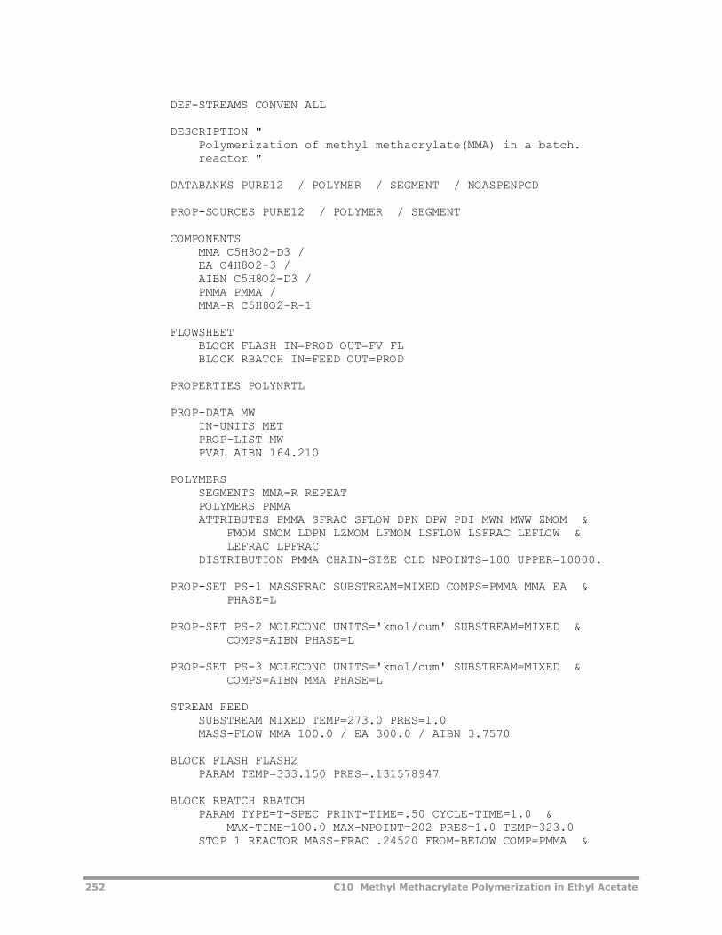
252 C10 Methyl Methacrylate Polymerization in Ethyl Acetate
DEF-STREAMS CONVEN ALL DESCRIPTION " Polymerization of methyl methacrylate(MMA) in a batch. reactor " DATABANKS PURE12 / POLYMER / SEGMENT / NOASPENPCD PROP-SOURCES PURE12 / POLYMER / SEGMENT COMPONENTS MMA C5H8O2-D3 / EA C4H8O2-3 / AIBN C5H8O2-D3 / PMMA PMMA / MMA-R C5H8O2-R-1 FLOWSHEET BLOCK FLASH IN=PROD OUT=FV FL BLOCK RBATCH IN=FEED OUT=PROD PROPERTIES POLYNRTL PROP-DATA MW IN-UNITS MET PROP-LIST MW PVAL AIBN 164.210 POLYMERS SEGMENTS MMA-R REPEAT POLYMERS PMMA ATTRIBUTES PMMA SFRAC SFLOW DPN DPW PDI MWN MWW ZMOM & FMOM SMOM LDPN LZMOM LFMOM LSFLOW LSFRAC LEFLOW & LEFRAC LPFRAC DISTRIBUTION PMMA CHAIN-SIZE CLD NPOINTS=100 UPPER=10000. PROP-SET PS-1 MASSFRAC SUBSTREAM=MIXED COMPS=PMMA MMA EA & PHASE=L PROP-SET PS-2 MOLECONC UNITS='kmol/cum' SUBSTREAM=MIXED & COMPS=AIBN PHASE=L PROP-SET PS-3 MOLECONC UNITS='kmol/cum' SUBSTREAM=MIXED & COMPS=AIBN MMA PHASE=L STREAM FEED SUBSTREAM MIXED TEMP=273.0 PRES=1.0 MASS-FLOW MMA 100.0 / EA 300.0 / AIBN 3.7570 BLOCK FLASH FLASH2 PARAM TEMP=333.150 PRES=.131578947 BLOCK RBATCH RBATCH PARAM TYPE=T-SPEC PRINT-TIME=.50 CYCLE-TIME=1.0 & MAX-TIME=100.0 MAX-NPOINT=202 PRES=1.0 TEMP=323.0 STOP 1 REACTOR MASS-FRAC .24520 FROM-BELOW COMP=PMMA &
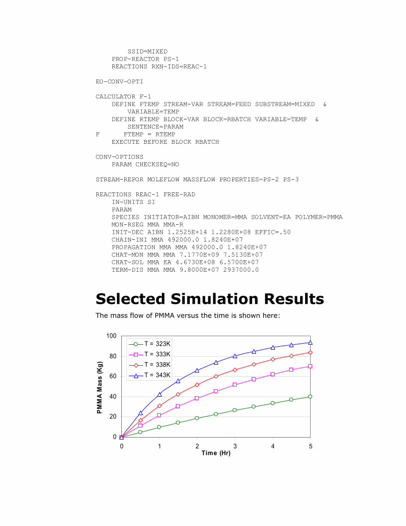
SSID=MIXED PROP-REACTOR PS-1 REACTIONS RXN-IDS=REAC-1 EO-CONV-OPTI CALCULATOR F-1 DEFINE FTEMP STREAM-VAR STREAM=FEED SUBSTREAM=MIXED & VARIABLE=TEMP DEFINE RTEMP BLOCK-VAR BLOCK=RBATCH VARIABLE=TEMP & SENTENCE=PARAM F FTEMP = RTEMP EXECUTE BEFORE BLOCK RBATCH CONV-OPTIONS PARAM CHECKSEQ=NO STREAM-REPOR MOLEFLOW MASSFLOW PROPERTIES=PS-2 PS-3 REACTIONS REAC-1 FREE-RAD IN-UNITS SI PARAM SPECIES INITIATOR=AIBN MONOMER=MMA SOLVENT=EA POLYMER=PMMA MON-RSEG MMA MMA-R INIT-DEC AIBN 1.2525E+14 1.2280E+08 EFFIC=.50 CHAIN-INI MMA 492000.0 1.8240E+07 PROPAGATION MMA MMA 492000.0 1.8240E+07 CHAT-MON MMA MMA 7.1770E+09 7.5130E+07 CHAT-SOL MMA EA 4.6730E+08 6.5700E+07 TERM-DIS MMA MMA 9.8000E+07 2937000.0
Selected Simulation Results The mass flow of PMMA versus the time is shown here:
0
20
40
60
80
100
0 1 2 3 4 5Time (Hr)
PMM
A M
ass
(Kg)
T = 323KT = 333KT = 338KT = 343K
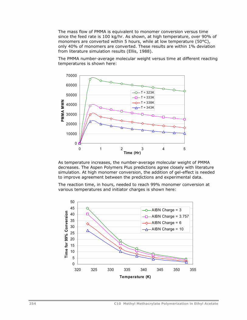
254 C10 Methyl Methacrylate Polymerization in Ethyl Acetate
The mass flow of PMMA is equivalent to monomer conversion versus time since the feed rate is 100 kg/hr. As shown, at high temperature, over 90% of monomers are converted within 5 hours, while at low temperature (50°C), only 40% of monomers are converted. These results are within 1% deviation from literature simulation results (Ellis, 1988).
The PMMA number-average molecular weight versus time at different reacting temperatures is shown here:
0
10000
20000
30000
40000
50000
60000
70000
0 1 2 3 4 5Time (Hr)
PMM
A M
WN
T = 323KT = 333KT = 338KT = 343K
As temperature increases, the number-average molecular weight of PMMA decreases. The Aspen Polymers Plus predictions agree closely with literature simulation. At high monomer conversion, the addition of gel-effect is needed to improve agreement between the predictions and experimental data.
The reaction time, in hours, needed to reach 99% monomer conversion at various temperatures and initiator charges is shown here:
05
101520253035404550
320 325 330 335 340 345 350 355
Temperature (K)
Tim
e fo
r 99
% C
onve
rsio
n AIBN Charge = 3AIBN Charge = 3.757AIBN Charge = 6AIBN Charge = 10
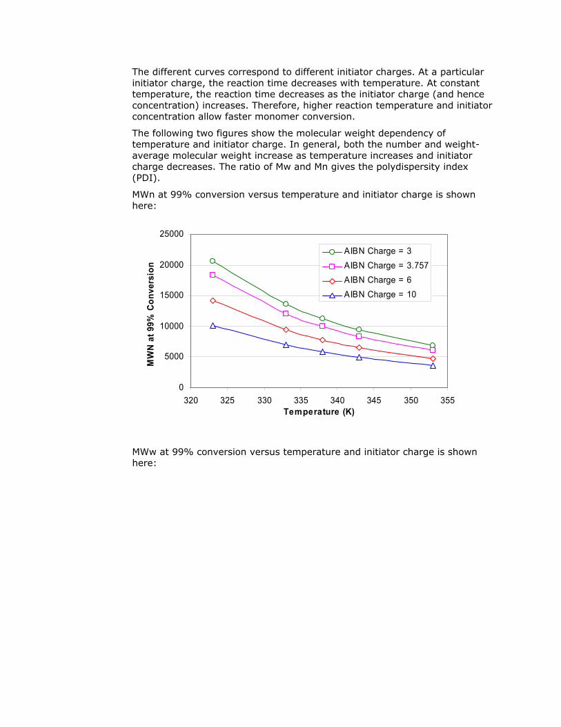
The different curves correspond to different initiator charges. At a particular initiator charge, the reaction time decreases with temperature. At constant temperature, the reaction time decreases as the initiator charge (and hence concentration) increases. Therefore, higher reaction temperature and initiator concentration allow faster monomer conversion.
The following two figures show the molecular weight dependency of temperature and initiator charge. In general, both the number and weight-average molecular weight increase as temperature increases and initiator charge decreases. The ratio of Mw and Mn gives the polydispersity index (PDI).
MWn at 99% conversion versus temperature and initiator charge is shown here:
0
5000
10000
15000
20000
25000
320 325 330 335 340 345 350 355Temperature (K)
MW
N at
99%
Con
vers
ion
AIBN Charge = 3AIBN Charge = 3.757AIBN Charge = 6AIBN Charge = 10
MWw at 99% conversion versus temperature and initiator charge is shown here:
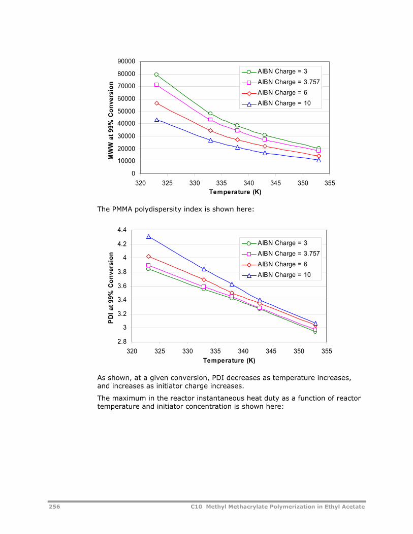
256 C10 Methyl Methacrylate Polymerization in Ethyl Acetate
0
10000
20000
30000
40000
50000
60000
70000
80000
90000
320 325 330 335 340 345 350 355Temperature (K)
MW
W a
t 99%
Con
vers
ion
AIBN Charge = 3AIBN Charge = 3.757AIBN Charge = 6AIBN Charge = 10
The PMMA polydispersity index is shown here:
2.8
3
3.2
3.4
3.6
3.8
4
4.2
4.4
320 325 330 335 340 345 350 355Temperature (K)
PDI a
t 99%
Con
vers
ion
AIBN Charge = 3AIBN Charge = 3.757AIBN Charge = 6AIBN Charge = 10
As shown, at a given conversion, PDI decreases as temperature increases, and increases as initiator charge increases.
The maximum in the reactor instantaneous heat duty as a function of reactor temperature and initiator concentration is shown here:
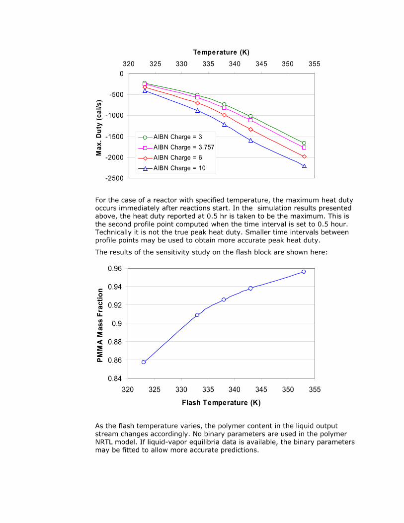
-2500
-2000
-1500
-1000
-500
0320 325 330 335 340 345 350 355
Temperature (K)
Max
. Dut
y (c
al/s
)
AIBN Charge = 3AIBN Charge = 3.757AIBN Charge = 6AIBN Charge = 10
For the case of a reactor with specified temperature, the maximum heat duty occurs immediately after reactions start. In the simulation results presented above, the heat duty reported at 0.5 hr is taken to be the maximum. This is the second profile point computed when the time interval is set to 0.5 hour. Technically it is not the true peak heat duty. Smaller time intervals between profile points may be used to obtain more accurate peak heat duty.
The results of the sensitivity study on the flash block are shown here:
0.84
0.86
0.88
0.9
0.92
0.94
0.96
320 325 330 335 340 345 350 355
Flash Temperature (K)
PMM
A M
ass
Frac
tion
As the flash temperature varies, the polymer content in the liquid output stream changes accordingly. No binary parameters are used in the polymer NRTL model. If liquid-vapor equilibria data is available, the binary parameters may be fitted to allow more accurate predictions.
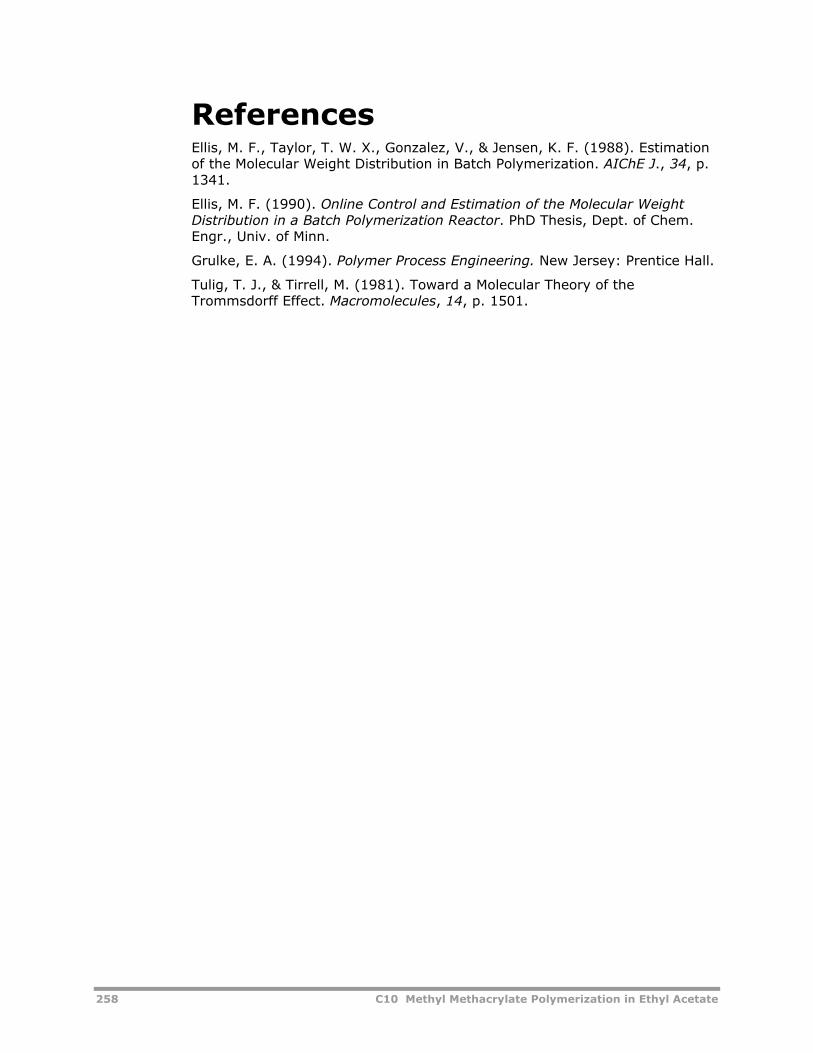
258 C10 Methyl Methacrylate Polymerization in Ethyl Acetate
References Ellis, M. F., Taylor, T. W. X., Gonzalez, V., & Jensen, K. F. (1988). Estimation of the Molecular Weight Distribution in Batch Polymerization. AIChE J., 34, p. 1341.
Ellis, M. F. (1990). Online Control and Estimation of the Molecular Weight Distribution in a Batch Polymerization Reactor. PhD Thesis, Dept. of Chem. Engr., Univ. of Minn.
Grulke, E. A. (1994). Polymer Process Engineering. New Jersey: Prentice Hall.
Tulig, T. J., & Tirrell, M. (1981). Toward a Molecular Theory of the Trommsdorff Effect. Macromolecules, 14, p. 1501.
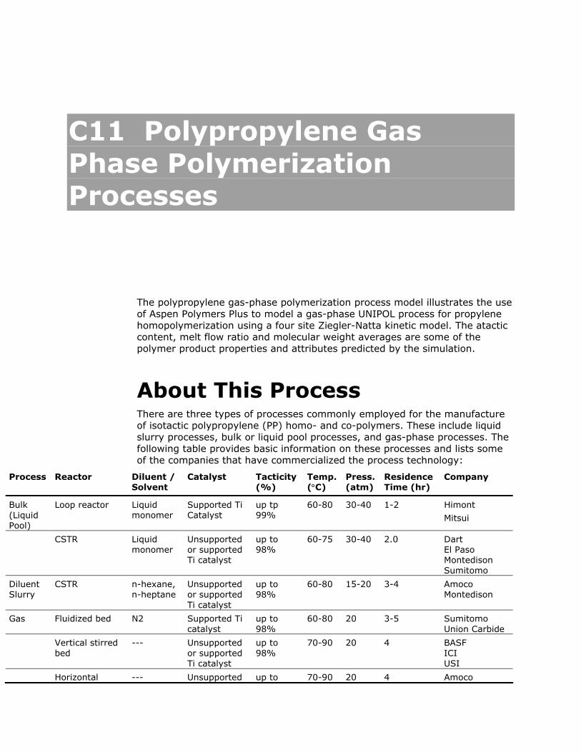
C11 Polypropylene Gas Phase Polymerization Processes
The polypropylene gas-phase polymerization process model illustrates the use of Aspen Polymers Plus to model a gas-phase UNIPOL process for propylene homopolymerization using a four site Ziegler-Natta kinetic model. The atactic content, melt flow ratio and molecular weight averages are some of the polymer product properties and attributes predicted by the simulation.
About This Process There are three types of processes commonly employed for the manufacture of isotactic polypropylene (PP) homo- and co-polymers. These include liquid slurry processes, bulk or liquid pool processes, and gas-phase processes. The following table provides basic information on these processes and lists some of the companies that have commercialized the process technology:
Process Reactor Diluent / Solvent
Catalyst Tacticity (%)
Temp. (°C)
Press. (atm)
Residence Time (hr)
Company
Bulk (Liquid Pool)
Loop reactor Liquid monomer
Supported Ti Catalyst
up tp 99%
60-80 30-40 1-2 Himont
Mitsui
CSTR Liquid monomer
Unsupported or supported Ti catalyst
up to 98%
60-75 30-40 2.0 Dart El Paso Montedison Sumitomo
Diluent Slurry
CSTR n-hexane, n-heptane
Unsupported or supported Ti catalyst
up to 98%
60-80 15-20 3-4 Amoco Montedison
Gas Fluidized bed N2 Supported Ti catalyst
up to 98%
60-80 20 3-5 Sumitomo Union Carbide
Vertical stirred bed
--- Unsupported or supported Ti catalyst
up to 98%
70-90 20 4 BASF ICI USI
Horizontal --- Unsupported up to 70-90 20 4 Amoco
260 C11 Polypropylene Gas Phase Polymerization Processes
Process Reactor Diluent / Solvent
Catalyst Tacticity (%)
Temp. (°C)
Press. (atm)
Residence Time (hr)
Company
compartmented stirred bed
or supported Ti catalyst
98%
All of these processes use a Ziegler-Natta catalyst (usually TiCl4) in either a supported or non-supported form together with an alkylaluminum or aluminum chlorides (for example, triethyl-aluminum) cocatalyst.
Liquid slurry processes use an inert hydrocarbon diluent as the slurry medium or polymer suspending agent. This process is still the most widely used process for PP manufacture. Continuous stirred tank reactors are usually used and several reactors may be used in series or parallel arrangements. Typical reactor operating conditions and residence times were listed in the previous table.
Bulk or liquid pool processes are a special case of the slurry processes. They use liquid propylene instead of an inert diluent as the slurry medium to suspend the polymer. The increased monomer concentration leads to higher polymerization rates in liquid pool processes relative to slurry processes. Hence, shorter reactor residence times may be employed. Several reactor types, including stirred autoclaves with evaporative cooling and loop reactors, are used to attain good heat transfer rates.
In gas-phase processes, gaseous propylene is contacted with solid catalyst/polymer powder in fluidized bed or mechanically stirred bed reactors. The reactor temperature is usually controlled by evaporative cooling of liquid propylene. The unreacted monomer is removed from the reactor headspace, condensed or cooled and recirculated to the reactor.
Aspen Polymers Plus can be used with Aspen Plus for the simulation of steady-state operation of any of the PP processes described above. Aspen Polymers Plus can be used with Aspen Custom Modeler when dynamic simulation or detailed modeling of the flow patterns or heat transfer within the reactor is desired. This example describes a steady-state simulation of a gas-phase UNIPOL flowsheet.
Process Definition An Aspen Polymers Plus model is developed to simulate a PP gas-phase UNIPOL flowsheet. The flowsheet includes the fluidized bed reactor, the gas recycle/cooling loop, discharge, and purge units:
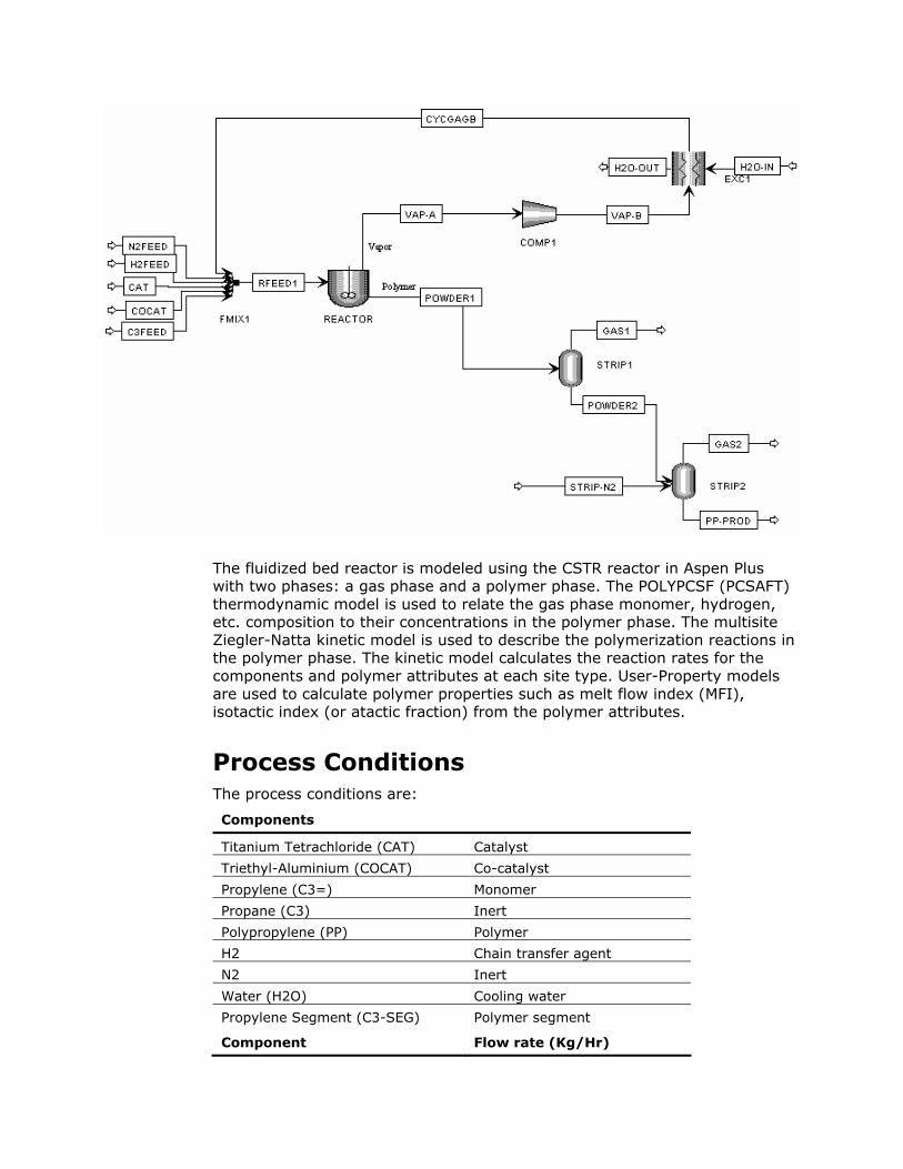
The fluidized bed reactor is modeled using the CSTR reactor in Aspen Plus with two phases: a gas phase and a polymer phase. The POLYPCSF (PCSAFT) thermodynamic model is used to relate the gas phase monomer, hydrogen, etc. composition to their concentrations in the polymer phase. The multisite Ziegler-Natta kinetic model is used to describe the polymerization reactions in the polymer phase. The kinetic model calculates the reaction rates for the components and polymer attributes at each site type. User-Property models are used to calculate polymer properties such as melt flow index (MFI), isotactic index (or atactic fraction) from the polymer attributes.
Process Conditions The process conditions are:
Components
Titanium Tetrachloride (CAT) Catalyst
Triethyl-Aluminium (COCAT) Co-catalyst
Propylene (C3=) Monomer
Propane (C3) Inert
Polypropylene (PP) Polymer
H2 Chain transfer agent
N2 Inert
Water (H2O) Cooling water
Propylene Segment (C3-SEG) Polymer segment
Component Flow rate (Kg/Hr)
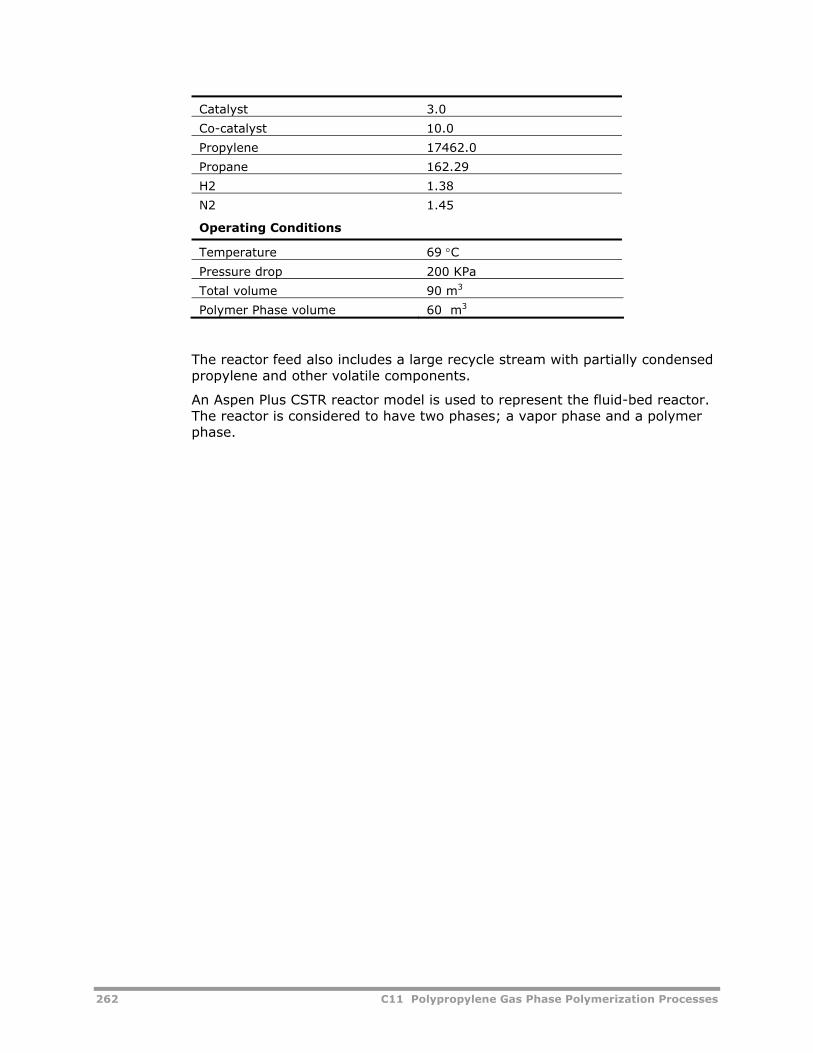
262 C11 Polypropylene Gas Phase Polymerization Processes
Catalyst 3.0
Co-catalyst 10.0
Propylene 17462.0
Propane 162.29
H2 1.38
N2 1.45
Operating Conditions
Temperature 69 °C
Pressure drop 200 KPa
Total volume 90 m3
Polymer Phase volume 60 m3
The reactor feed also includes a large recycle stream with partially condensed propylene and other volatile components.
An Aspen Plus CSTR reactor model is used to represent the fluid-bed reactor. The reactor is considered to have two phases; a vapor phase and a polymer phase.
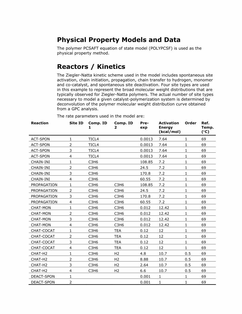
Physical Property Models and Data The polymer PCSAFT equation of state model (POLYPCSF) is used as the physical property method.
Reactors / Kinetics The Ziegler-Natta kinetic scheme used in the model includes spontaneous site activation, chain initiation, propagation, chain transfer to hydrogen, monomer and co-catalyst, and spontaneous site deactivation. Four site types are used in this example to represent the broad molecular weight distributions that are typically observed for Ziegler-Natta polymers. The actual number of site types necessary to model a given catalyst-polymerization system is determined by deconvolution of the polymer molecular weight distribution curve obtained from a GPC analysis.
The rate parameters used in the model are:
Reaction Site ID Comp. ID 1
Comp. ID 2
Pre-exp
Activation Energy (kcal/mol)
Order Ref. Temp. (°C)
ACT-SPON 1 TICL4 0.0013 7.64 1 69
ACT-SPON 2 TICL4 0.0013 7.64 1 69
ACT-SPON 3 TICL4 0.0013 7.64 1 69
ACT-SPON 4 TICL4 0.0013 7.64 1 69
CHAIN-INI 1 C3H6 108.85 7.2 1 69
CHAIN-INI 2 C3H6 24.5 7.2 1 69
CHAIN-INI 3 C3H6 170.8 7.2 1 69
CHAIN-INI 4 C3H6 60.55 7.2 1 69
PROPAGATION 1 C3H6 C3H6 108.85 7.2 1 69
PROPAGATION 2 C3H6 C3H6 24.5 7.2 1 69
PROPAGATION 3 C3H6 C3H6 170.8 7.2 1 69
PROPAGATION 4 C3H6 C3H6 60.55 7.2 1 69
CHAT-MON 1 C3H6 C3H6 0.012 12.42 1 69
CHAT-MON 2 C3H6 C3H6 0.012 12.42 1 69
CHAT-MON 3 C3H6 C3H6 0.012 12.42 1 69
CHAT-MON 4 C3H6 C3H6 0.012 12.42 1 69
CHAT-COCAT 1 C3H6 TEA 0.12 12 1 69
CHAT-COCAT 2 C3H6 TEA 0.12 12 1 69
CHAT-COCAT 3 C3H6 TEA 0.12 12 1 69
CHAT-COCAT 4 C3H6 TEA 0.12 12 1 69
CHAT-H2 1 C3H6 H2 4.8 10.7 0.5 69
CHAT-H2 2 C3H6 H2 8.88 10.7 0.5 69
CHAT-H2 3 C3H6 H2 2.64 10.7 0.5 69
CHAT-H2 4 C3H6 H2 6.6 10.7 0.5 69
DEACT-SPON 1 0.001 1 1 69
DEACT-SPON 2 0.001 1 1 69
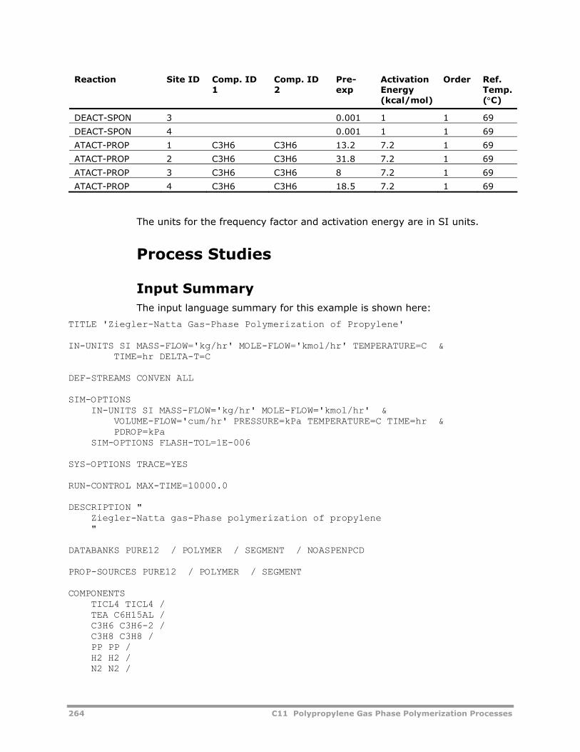
264 C11 Polypropylene Gas Phase Polymerization Processes
Reaction Site ID Comp. ID 1
Comp. ID 2
Pre-exp
Activation Energy (kcal/mol)
Order Ref. Temp. (°C)
DEACT-SPON 3 0.001 1 1 69
DEACT-SPON 4 0.001 1 1 69
ATACT-PROP 1 C3H6 C3H6 13.2 7.2 1 69
ATACT-PROP 2 C3H6 C3H6 31.8 7.2 1 69
ATACT-PROP 3 C3H6 C3H6 8 7.2 1 69
ATACT-PROP 4 C3H6 C3H6 18.5 7.2 1 69
The units for the frequency factor and activation energy are in SI units.
Process Studies
Input Summary The input language summary for this example is shown here:
TITLE 'Ziegler-Natta Gas-Phase Polymerization of Propylene' IN-UNITS SI MASS-FLOW='kg/hr' MOLE-FLOW='kmol/hr' TEMPERATURE=C & TIME=hr DELTA-T=C DEF-STREAMS CONVEN ALL SIM-OPTIONS IN-UNITS SI MASS-FLOW='kg/hr' MOLE-FLOW='kmol/hr' & VOLUME-FLOW='cum/hr' PRESSURE=kPa TEMPERATURE=C TIME=hr & PDROP=kPa SIM-OPTIONS FLASH-TOL=1E-006 SYS-OPTIONS TRACE=YES RUN-CONTROL MAX-TIME=10000.0 DESCRIPTION " Ziegler-Natta gas-Phase polymerization of propylene " DATABANKS PURE12 / POLYMER / SEGMENT / NOASPENPCD PROP-SOURCES PURE12 / POLYMER / SEGMENT COMPONENTS TICL4 TICL4 / TEA C6H15AL / C3H6 C3H6-2 / C3H8 C3H8 / PP PP / H2 H2 / N2 N2 /
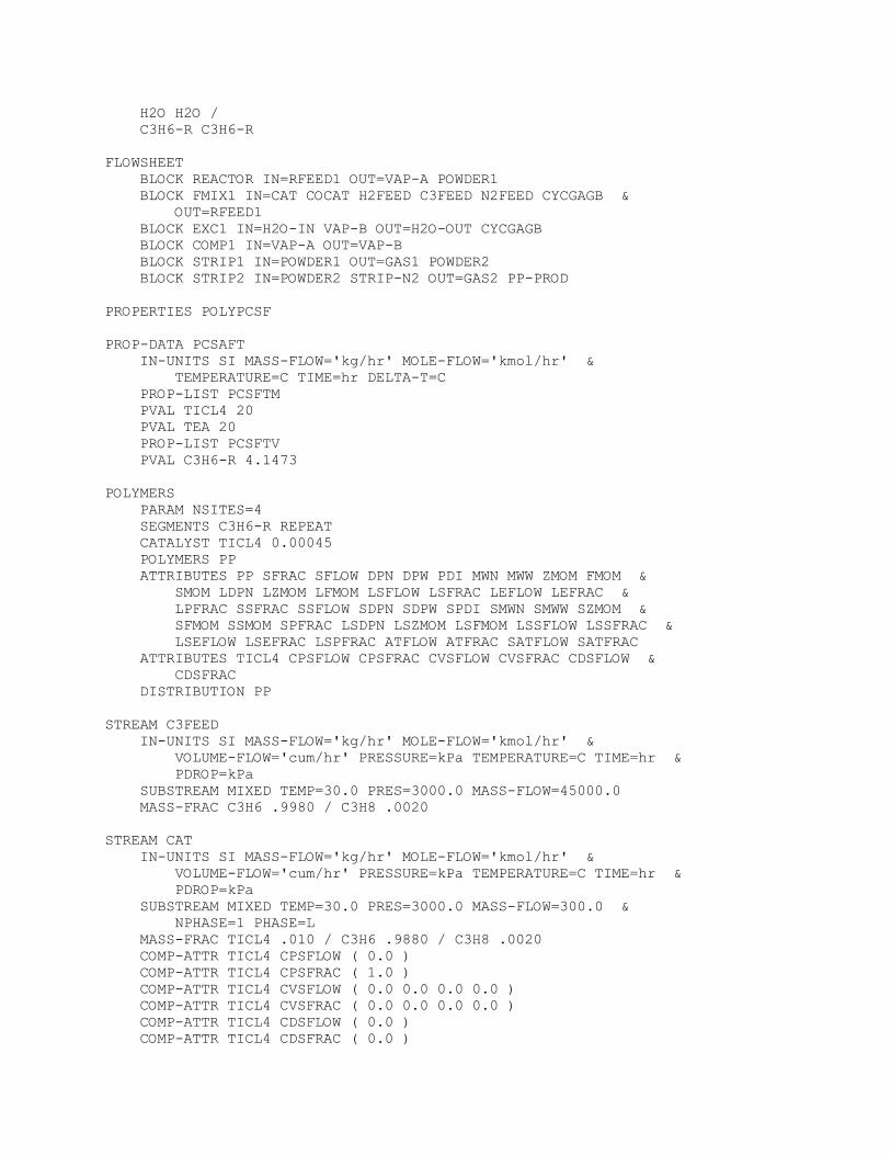
H2O H2O / C3H6-R C3H6-R FLOWSHEET BLOCK REACTOR IN=RFEED1 OUT=VAP-A POWDER1 BLOCK FMIX1 IN=CAT COCAT H2FEED C3FEED N2FEED CYCGAGB & OUT=RFEED1 BLOCK EXC1 IN=H2O-IN VAP-B OUT=H2O-OUT CYCGAGB BLOCK COMP1 IN=VAP-A OUT=VAP-B BLOCK STRIP1 IN=POWDER1 OUT=GAS1 POWDER2 BLOCK STRIP2 IN=POWDER2 STRIP-N2 OUT=GAS2 PP-PROD PROPERTIES POLYPCSF PROP-DATA PCSAFT IN-UNITS SI MASS-FLOW='kg/hr' MOLE-FLOW='kmol/hr' & TEMPERATURE=C TIME=hr DELTA-T=C PROP-LIST PCSFTM PVAL TICL4 20 PVAL TEA 20 PROP-LIST PCSFTV PVAL C3H6-R 4.1473 POLYMERS PARAM NSITES=4 SEGMENTS C3H6-R REPEAT CATALYST TICL4 0.00045 POLYMERS PP ATTRIBUTES PP SFRAC SFLOW DPN DPW PDI MWN MWW ZMOM FMOM & SMOM LDPN LZMOM LFMOM LSFLOW LSFRAC LEFLOW LEFRAC & LPFRAC SSFRAC SSFLOW SDPN SDPW SPDI SMWN SMWW SZMOM & SFMOM SSMOM SPFRAC LSDPN LSZMOM LSFMOM LSSFLOW LSSFRAC & LSEFLOW LSEFRAC LSPFRAC ATFLOW ATFRAC SATFLOW SATFRAC ATTRIBUTES TICL4 CPSFLOW CPSFRAC CVSFLOW CVSFRAC CDSFLOW & CDSFRAC DISTRIBUTION PP STREAM C3FEED IN-UNITS SI MASS-FLOW='kg/hr' MOLE-FLOW='kmol/hr' & VOLUME-FLOW='cum/hr' PRESSURE=kPa TEMPERATURE=C TIME=hr & PDROP=kPa SUBSTREAM MIXED TEMP=30.0 PRES=3000.0 MASS-FLOW=45000.0 MASS-FRAC C3H6 .9980 / C3H8 .0020 STREAM CAT IN-UNITS SI MASS-FLOW='kg/hr' MOLE-FLOW='kmol/hr' & VOLUME-FLOW='cum/hr' PRESSURE=kPa TEMPERATURE=C TIME=hr & PDROP=kPa SUBSTREAM MIXED TEMP=30.0 PRES=3000.0 MASS-FLOW=300.0 & NPHASE=1 PHASE=L MASS-FRAC TICL4 .010 / C3H6 .9880 / C3H8 .0020 COMP-ATTR TICL4 CPSFLOW ( 0.0 ) COMP-ATTR TICL4 CPSFRAC ( 1.0 ) COMP-ATTR TICL4 CVSFLOW ( 0.0 0.0 0.0 0.0 ) COMP-ATTR TICL4 CVSFRAC ( 0.0 0.0 0.0 0.0 ) COMP-ATTR TICL4 CDSFLOW ( 0.0 ) COMP-ATTR TICL4 CDSFRAC ( 0.0 )
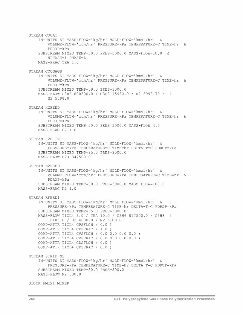
266 C11 Polypropylene Gas Phase Polymerization Processes
STREAM COCAT IN-UNITS SI MASS-FLOW='kg/hr' MOLE-FLOW='kmol/hr' & VOLUME-FLOW='cum/hr' PRESSURE=kPa TEMPERATURE=C TIME=hr & PDROP=kPa SUBSTREAM MIXED TEMP=30.0 PRES=3000.0 MASS-FLOW=10.0 & NPHASE=1 PHASE=L MASS-FRAC TEA 1.0 STREAM CYCGAGB IN-UNITS SI MASS-FLOW='kg/hr' MOLE-FLOW='kmol/hr' & VOLUME-FLOW='cum/hr' PRESSURE=kPa TEMPERATURE=C TIME=hr & PDROP=kPa SUBSTREAM MIXED TEMP=59.0 PRES=3000.0 MASS-FLOW C3H6 800300.0 / C3H8 15930.0 / H2 3998.70 / & N2 5098.0 STREAM H2FEED IN-UNITS SI MASS-FLOW='kg/hr' MOLE-FLOW='kmol/hr' & VOLUME-FLOW='cum/hr' PRESSURE=kPa TEMPERATURE=C TIME=hr & PDROP=kPa SUBSTREAM MIXED TEMP=30.0 PRES=3000.0 MASS-FLOW=4.0 MASS-FRAC H2 1.0 STREAM H2O-IN IN-UNITS SI MASS-FLOW='kg/hr' MOLE-FLOW='kmol/hr' & PRESSURE=kPa TEMPERATURE=C TIME=hr DELTA-T=C PDROP=kPa SUBSTREAM MIXED TEMP=35.0 PRES=3000.0 MASS-FLOW H2O 847500.0 STREAM N2FEED IN-UNITS SI MASS-FLOW='kg/hr' MOLE-FLOW='kmol/hr' & VOLUME-FLOW='cum/hr' PRESSURE=kPa TEMPERATURE=C TIME=hr & PDROP=kPa SUBSTREAM MIXED TEMP=30.0 PRES=3000.0 MASS-FLOW=100.0 MASS-FRAC N2 1.0 STREAM RFEED1 IN-UNITS SI MASS-FLOW='kg/hr' MOLE-FLOW='kmol/hr' & PRESSURE=kPa TEMPERATURE=C TIME=hr DELTA-T=C PDROP=kPa SUBSTREAM MIXED TEMP=65.0 PRES=3000.0 MASS-FLOW TICL4 3.0 / TEA 10.0 / C3H6 817500.0 / C3H8 & 16100.0 / H2 4000.0 / N2 5100.0 COMP-ATTR TICL4 CPSFLOW ( 0.0 ) COMP-ATTR TICL4 CPSFRAC ( 1.0 ) COMP-ATTR TICL4 CVSFLOW ( 0.0 0.0 0.0 0.0 ) COMP-ATTR TICL4 CVSFRAC ( 0.0 0.0 0.0 0.0 ) COMP-ATTR TICL4 CDSFLOW ( 0.0 ) COMP-ATTR TICL4 CDSFRAC ( 0.0 ) STREAM STRIP-N2 IN-UNITS SI MASS-FLOW='kg/hr' MOLE-FLOW='kmol/hr' & PRESSURE=kPa TEMPERATURE=C TIME=hr DELTA-T=C PDROP=kPa SUBSTREAM MIXED TEMP=30.0 PRES=300.0 MASS-FLOW N2 500.0 BLOCK FMIX1 MIXER
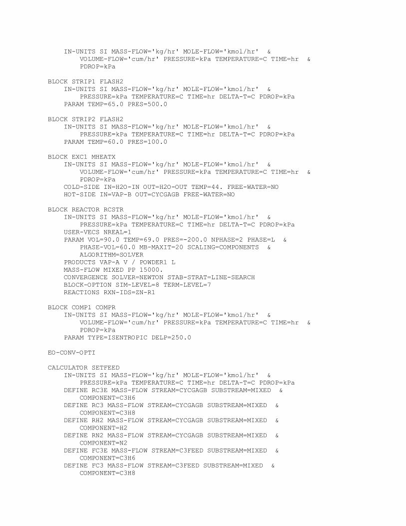
IN-UNITS SI MASS-FLOW='kg/hr' MOLE-FLOW='kmol/hr' & VOLUME-FLOW='cum/hr' PRESSURE=kPa TEMPERATURE=C TIME=hr & PDROP=kPa BLOCK STRIP1 FLASH2 IN-UNITS SI MASS-FLOW='kg/hr' MOLE-FLOW='kmol/hr' & PRESSURE=kPa TEMPERATURE=C TIME=hr DELTA-T=C PDROP=kPa PARAM TEMP=65.0 PRES=500.0 BLOCK STRIP2 FLASH2 IN-UNITS SI MASS-FLOW='kg/hr' MOLE-FLOW='kmol/hr' & PRESSURE=kPa TEMPERATURE=C TIME=hr DELTA-T=C PDROP=kPa PARAM TEMP=60.0 PRES=100.0 BLOCK EXC1 MHEATX IN-UNITS SI MASS-FLOW='kg/hr' MOLE-FLOW='kmol/hr' & VOLUME-FLOW='cum/hr' PRESSURE=kPa TEMPERATURE=C TIME=hr & PDROP=kPa COLD-SIDE IN=H2O-IN OUT=H2O-OUT TEMP=44. FREE-WATER=NO HOT-SIDE IN=VAP-B OUT=CYCGAGB FREE-WATER=NO BLOCK REACTOR RCSTR IN-UNITS SI MASS-FLOW='kg/hr' MOLE-FLOW='kmol/hr' & PRESSURE=kPa TEMPERATURE=C TIME=hr DELTA-T=C PDROP=kPa USER-VECS NREAL=1 PARAM VOL=90.0 TEMP=69.0 PRES=-200.0 NPHASE=2 PHASE=L & PHASE-VOL=60.0 MB-MAXIT=20 SCALING=COMPONENTS & ALGORITHM=SOLVER PRODUCTS VAP-A V / POWDER1 L MASS-FLOW MIXED PP 15000. CONVERGENCE SOLVER=NEWTON STAB-STRAT=LINE-SEARCH BLOCK-OPTION SIM-LEVEL=8 TERM-LEVEL=7 REACTIONS RXN-IDS=ZN-R1 BLOCK COMP1 COMPR IN-UNITS SI MASS-FLOW='kg/hr' MOLE-FLOW='kmol/hr' & VOLUME-FLOW='cum/hr' PRESSURE=kPa TEMPERATURE=C TIME=hr & PDROP=kPa PARAM TYPE=ISENTROPIC DELP=250.0 EO-CONV-OPTI CALCULATOR SETFEED IN-UNITS SI MASS-FLOW='kg/hr' MOLE-FLOW='kmol/hr' & PRESSURE=kPa TEMPERATURE=C TIME=hr DELTA-T=C PDROP=kPa DEFINE RC3E MASS-FLOW STREAM=CYCGAGB SUBSTREAM=MIXED & COMPONENT=C3H6 DEFINE RC3 MASS-FLOW STREAM=CYCGAGB SUBSTREAM=MIXED & COMPONENT=C3H8 DEFINE RH2 MASS-FLOW STREAM=CYCGAGB SUBSTREAM=MIXED & COMPONENT=H2 DEFINE RN2 MASS-FLOW STREAM=CYCGAGB SUBSTREAM=MIXED & COMPONENT=N2 DEFINE FC3E MASS-FLOW STREAM=C3FEED SUBSTREAM=MIXED & COMPONENT=C3H6 DEFINE FC3 MASS-FLOW STREAM=C3FEED SUBSTREAM=MIXED & COMPONENT=C3H8
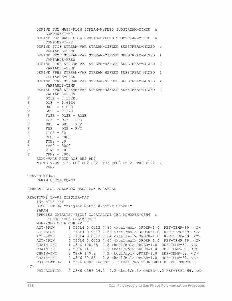
268 C11 Polypropylene Gas Phase Polymerization Processes
DEFINE FN2 MASS-FLOW STREAM=N2FEED SUBSTREAM=MIXED & COMPONENT=N2 DEFINE FH2 MASS-FLOW STREAM=H2FEED SUBSTREAM=MIXED & COMPONENT=H2 DEFINE FTC3 STREAM-VAR STREAM=C3FEED SUBSTREAM=MIXED & VARIABLE=TEMP DEFINE FPC3 STREAM-VAR STREAM=C3FEED SUBSTREAM=MIXED & VARIABLE=PRES DEFINE FTH2 STREAM-VAR STREAM=H2FEED SUBSTREAM=MIXED & VARIABLE=TEMP DEFINE FPH2 STREAM-VAR STREAM=H2FEED SUBSTREAM=MIXED & VARIABLE=PRES DEFINE FTN2 STREAM-VAR STREAM=N2FEED SUBSTREAM=MIXED & VARIABLE=TEMP DEFINE FPN2 STREAM-VAR STREAM=N2FEED SUBSTREAM=MIXED & VARIABLE=PRES F DC3E = 8.172E5 F DC3 = 1.61E4 F DH2 = 4.0E3 F DN2 = 5.1E3 F FC3E = DC3E - RC3E F FC3 = DC3 - RC3 F FH2 = DH2 - RH2 F FN2 = DN2 - RN2 F FTC3 = 30 F FPC3 = 3000 F FTH2 = 30 F FPH2 = 3000 F FTN2 = 30 F FPN2 = 3000 READ-VARS RC3E RC3 RH2 RN2 WRITE-VARS FC3E FC3 FN2 FH2 FTC3 FPC3 FTH2 FPH2 FTN2 & FPN2 CONV-OPTIONS PARAM CHECKSEQ=NO STREAM-REPOR MOLEFLOW MASSFLOW MASSFRAC REACTIONS ZN-R1 ZIEGLER-NAT IN-UNITS MET DESCRIPTION "Ziegler-Natta Kinetic Scheme" PARAM SPECIES CATALYST=TICL4 COCATALYST=TEA MONOMER=C3H6 & HYDROGEN=H2 POLYMER=PP MON-RSEG C3H6 C3H6-R ACT-SPON 1 TICL4 0.0013 7.64 <kcal/mol> ORDER=1.0 REF-TEMP=69. <C> ACT-SPON 2 TICL4 0.0013 7.64 <kcal/mol> ORDER=1.0 REF-TEMP=69. <C> ACT-SPON 3 TICL4 0.0013 7.64 <kcal/mol> ORDER=1.0 REF-TEMP=69. <C> ACT-SPON 4 TICL4 0.0013 7.64 <kcal/mol> ORDER=1.0 REF-TEMP=69. <C> CHAIN-INI 1 C3H6 108.85 7.2 <kcal/mol> ORDER=1.0 REF-TEMP=69. <C> CHAIN-INI 2 C3H6 24.5 7.2 <kcal/mol> ORDER=1.0 REF-TEMP=69. <C> CHAIN-INI 3 C3H6 170.8 7.2 <kcal/mol> ORDER=1.0 REF-TEMP=69. <C> CHAIN-INI 4 C3H6 60.55 7.2 <kcal/mol> ORDER=1.0 REF-TEMP=69. <C> PROPAGATION 1 C3H6 C3H6 108.85 7.2 <kcal/mol> ORDER=1.0 REF-TEMP=69. <C> PROPAGATION 2 C3H6 C3H6 24.5 7.2 <kcal/mol> ORDER=1.0 REF-TEMP=69. <C>
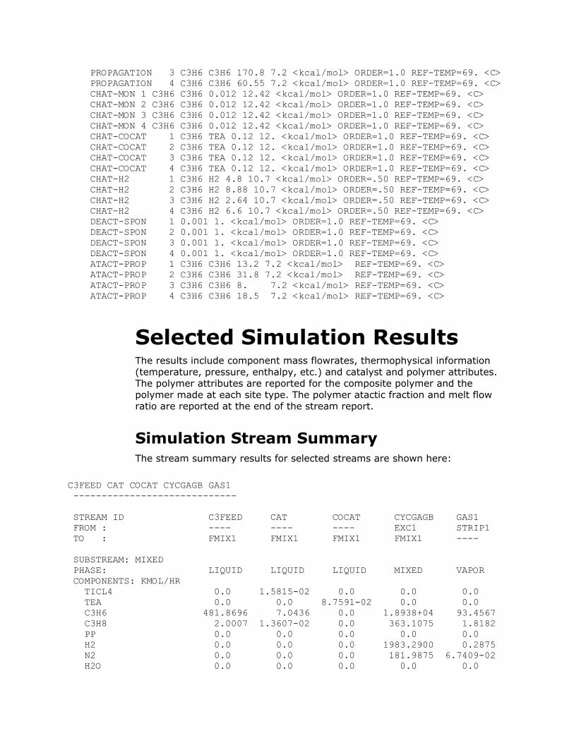
PROPAGATION 3 C3H6 C3H6 170.8 7.2 <kcal/mol> ORDER=1.0 REF-TEMP=69. <C> PROPAGATION 4 C3H6 C3H6 60.55 7.2 <kcal/mol> ORDER=1.0 REF-TEMP=69. <C> CHAT-MON 1 C3H6 C3H6 0.012 12.42 <kcal/mol> ORDER=1.0 REF-TEMP=69. <C> CHAT-MON 2 C3H6 C3H6 0.012 12.42 <kcal/mol> ORDER=1.0 REF-TEMP=69. <C> CHAT-MON 3 C3H6 C3H6 0.012 12.42 <kcal/mol> ORDER=1.0 REF-TEMP=69. <C> CHAT-MON 4 C3H6 C3H6 0.012 12.42 <kcal/mol> ORDER=1.0 REF-TEMP=69. <C> CHAT-COCAT 1 C3H6 TEA 0.12 12. <kcal/mol> ORDER=1.0 REF-TEMP=69. <C> CHAT-COCAT 2 C3H6 TEA 0.12 12. <kcal/mol> ORDER=1.0 REF-TEMP=69. <C> CHAT-COCAT 3 C3H6 TEA 0.12 12. <kcal/mol> ORDER=1.0 REF-TEMP=69. <C> CHAT-COCAT 4 C3H6 TEA 0.12 12. <kcal/mol> ORDER=1.0 REF-TEMP=69. <C> CHAT-H2 1 C3H6 H2 4.8 10.7 <kcal/mol> ORDER=.50 REF-TEMP=69. <C> CHAT-H2 2 C3H6 H2 8.88 10.7 <kcal/mol> ORDER=.50 REF-TEMP=69. <C> CHAT-H2 3 C3H6 H2 2.64 10.7 <kcal/mol> ORDER=.50 REF-TEMP=69. <C> CHAT-H2 4 C3H6 H2 6.6 10.7 <kcal/mol> ORDER=.50 REF-TEMP=69. <C> DEACT-SPON 1 0.001 1. <kcal/mol> ORDER=1.0 REF-TEMP=69. <C> DEACT-SPON 2 0.001 1. <kcal/mol> ORDER=1.0 REF-TEMP=69. <C> DEACT-SPON 3 0.001 1. <kcal/mol> ORDER=1.0 REF-TEMP=69. <C> DEACT-SPON 4 0.001 1. <kcal/mol> ORDER=1.0 REF-TEMP=69. <C> ATACT-PROP 1 C3H6 C3H6 13.2 7.2 <kcal/mol> REF-TEMP=69. <C> ATACT-PROP 2 C3H6 C3H6 31.8 7.2 <kcal/mol> REF-TEMP=69. <C> ATACT-PROP 3 C3H6 C3H6 8. 7.2 <kcal/mol> REF-TEMP=69. <C> ATACT-PROP 4 C3H6 C3H6 18.5 7.2 <kcal/mol> REF-TEMP=69. <C>
Selected Simulation Results The results include component mass flowrates, thermophysical information (temperature, pressure, enthalpy, etc.) and catalyst and polymer attributes. The polymer attributes are reported for the composite polymer and the polymer made at each site type. The polymer atactic fraction and melt flow ratio are reported at the end of the stream report.
Simulation Stream Summary The stream summary results for selected streams are shown here:
C3FEED CAT COCAT CYCGAGB GAS1 ----------------------------- STREAM ID C3FEED CAT COCAT CYCGAGB GAS1 FROM : ---- ---- ---- EXC1 STRIP1 TO : FMIX1 FMIX1 FMIX1 FMIX1 ---- SUBSTREAM: MIXED PHASE: LIQUID LIQUID LIQUID MIXED VAPOR COMPONENTS: KMOL/HR TICL4 0.0 1.5815-02 0.0 0.0 0.0 TEA 0.0 0.0 8.7591-02 0.0 0.0 C3H6 481.8696 7.0436 0.0 1.8938+04 93.4567 C3H8 2.0007 1.3607-02 0.0 363.1075 1.8182 PP 0.0 0.0 0.0 0.0 0.0 H2 0.0 0.0 0.0 1983.2900 0.2875 N2 0.0 0.0 0.0 181.9875 6.7409-02 H2O 0.0 0.0 0.0 0.0 0.0
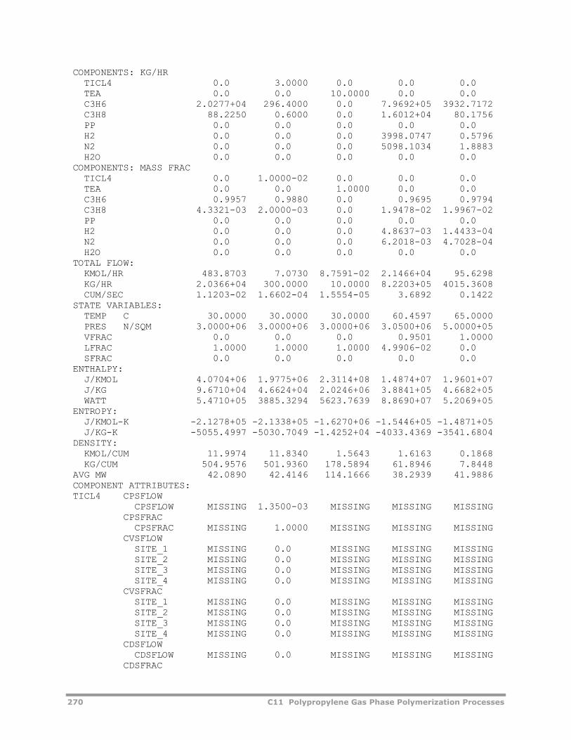
270 C11 Polypropylene Gas Phase Polymerization Processes
COMPONENTS: KG/HR TICL4 0.0 3.0000 0.0 0.0 0.0 TEA 0.0 0.0 10.0000 0.0 0.0 C3H6 2.0277+04 296.4000 0.0 7.9692+05 3932.7172 C3H8 88.2250 0.6000 0.0 1.6012+04 80.1756 PP 0.0 0.0 0.0 0.0 0.0 H2 0.0 0.0 0.0 3998.0747 0.5796 N2 0.0 0.0 0.0 5098.1034 1.8883 H2O 0.0 0.0 0.0 0.0 0.0 COMPONENTS: MASS FRAC TICL4 0.0 1.0000-02 0.0 0.0 0.0 TEA 0.0 0.0 1.0000 0.0 0.0 C3H6 0.9957 0.9880 0.0 0.9695 0.9794 C3H8 4.3321-03 2.0000-03 0.0 1.9478-02 1.9967-02 PP 0.0 0.0 0.0 0.0 0.0 H2 0.0 0.0 0.0 4.8637-03 1.4433-04 N2 0.0 0.0 0.0 6.2018-03 4.7028-04 H2O 0.0 0.0 0.0 0.0 0.0 TOTAL FLOW: KMOL/HR 483.8703 7.0730 8.7591-02 2.1466+04 95.6298 KG/HR 2.0366+04 300.0000 10.0000 8.2203+05 4015.3608 CUM/SEC 1.1203-02 1.6602-04 1.5554-05 3.6892 0.1422 STATE VARIABLES: TEMP C 30.0000 30.0000 30.0000 60.4597 65.0000 PRES N/SQM 3.0000+06 3.0000+06 3.0000+06 3.0500+06 5.0000+05 VFRAC 0.0 0.0 0.0 0.9501 1.0000 LFRAC 1.0000 1.0000 1.0000 4.9906-02 0.0 SFRAC 0.0 0.0 0.0 0.0 0.0 ENTHALPY: J/KMOL 4.0704+06 1.9775+06 2.3114+08 1.4874+07 1.9601+07 J/KG 9.6710+04 4.6624+04 2.0246+06 3.8841+05 4.6682+05 WATT 5.4710+05 3885.3294 5623.7639 8.8690+07 5.2069+05 ENTROPY: J/KMOL-K -2.1278+05 -2.1338+05 -1.6270+06 -1.5446+05 -1.4871+05 J/KG-K -5055.4997 -5030.7049 -1.4252+04 -4033.4369 -3541.6804 DENSITY: KMOL/CUM 11.9974 11.8340 1.5643 1.6163 0.1868 KG/CUM 504.9576 501.9360 178.5894 61.8946 7.8448 AVG MW 42.0890 42.4146 114.1666 38.2939 41.9886 COMPONENT ATTRIBUTES: TICL4 CPSFLOW CPSFLOW MISSING 1.3500-03 MISSING MISSING MISSING CPSFRAC CPSFRAC MISSING 1.0000 MISSING MISSING MISSING CVSFLOW SITE_1 MISSING 0.0 MISSING MISSING MISSING SITE_2 MISSING 0.0 MISSING MISSING MISSING SITE_3 MISSING 0.0 MISSING MISSING MISSING SITE_4 MISSING 0.0 MISSING MISSING MISSING CVSFRAC SITE_1 MISSING 0.0 MISSING MISSING MISSING SITE_2 MISSING 0.0 MISSING MISSING MISSING SITE_3 MISSING 0.0 MISSING MISSING MISSING SITE_4 MISSING 0.0 MISSING MISSING MISSING CDSFLOW CDSFLOW MISSING 0.0 MISSING MISSING MISSING CDSFRAC
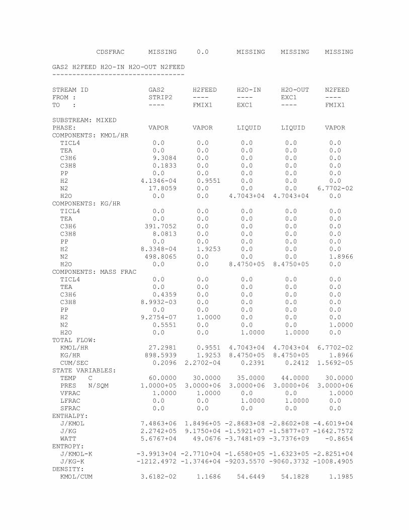
CDSFRAC MISSING 0.0 MISSING MISSING MISSING GAS2 H2FEED H2O-IN H2O-OUT N2FEED --------------------------------- STREAM ID GAS2 H2FEED H2O-IN H2O-OUT N2FEED FROM : STRIP2 ---- ---- EXC1 ---- TO : ---- FMIX1 EXC1 ---- FMIX1 SUBSTREAM: MIXED PHASE: VAPOR VAPOR LIQUID LIQUID VAPOR COMPONENTS: KMOL/HR TICL4 0.0 0.0 0.0 0.0 0.0 TEA 0.0 0.0 0.0 0.0 0.0 C3H6 9.3084 0.0 0.0 0.0 0.0 C3H8 0.1833 0.0 0.0 0.0 0.0 PP 0.0 0.0 0.0 0.0 0.0 H2 4.1346-04 0.9551 0.0 0.0 0.0 N2 17.8059 0.0 0.0 0.0 6.7702-02 H2O 0.0 0.0 4.7043+04 4.7043+04 0.0 COMPONENTS: KG/HR TICL4 0.0 0.0 0.0 0.0 0.0 TEA 0.0 0.0 0.0 0.0 0.0 C3H6 391.7052 0.0 0.0 0.0 0.0 C3H8 8.0813 0.0 0.0 0.0 0.0 PP 0.0 0.0 0.0 0.0 0.0 H2 8.3348-04 1.9253 0.0 0.0 0.0 N2 498.8065 0.0 0.0 0.0 1.8966 H2O 0.0 0.0 8.4750+05 8.4750+05 0.0 COMPONENTS: MASS FRAC TICL4 0.0 0.0 0.0 0.0 0.0 TEA 0.0 0.0 0.0 0.0 0.0 C3H6 0.4359 0.0 0.0 0.0 0.0 C3H8 8.9932-03 0.0 0.0 0.0 0.0 PP 0.0 0.0 0.0 0.0 0.0 H2 9.2754-07 1.0000 0.0 0.0 0.0 N2 0.5551 0.0 0.0 0.0 1.0000 H2O 0.0 0.0 1.0000 1.0000 0.0 TOTAL FLOW: KMOL/HR 27.2981 0.9551 4.7043+04 4.7043+04 6.7702-02 KG/HR 898.5939 1.9253 8.4750+05 8.4750+05 1.8966 CUM/SEC 0.2096 2.2702-04 0.2391 0.2412 1.5692-05 STATE VARIABLES: TEMP C 60.0000 30.0000 35.0000 44.0000 30.0000 PRES N/SQM 1.0000+05 3.0000+06 3.0000+06 3.0000+06 3.0000+06 VFRAC 1.0000 1.0000 0.0 0.0 1.0000 LFRAC 0.0 0.0 1.0000 1.0000 0.0 SFRAC 0.0 0.0 0.0 0.0 0.0 ENTHALPY: J/KMOL 7.4863+06 1.8496+05 -2.8683+08 -2.8602+08 -4.6019+04 J/KG 2.2742+05 9.1750+04 -1.5921+07 -1.5877+07 -1642.7572 WATT 5.6767+04 49.0676 -3.7481+09 -3.7376+09 -0.8654 ENTROPY: J/KMOL-K -3.9913+04 -2.7710+04 -1.6580+05 -1.6323+05 -2.8251+04 J/KG-K -1212.4972 -1.3746+04 -9203.5570 -9060.3732 -1008.4905 DENSITY: KMOL/CUM 3.6182-02 1.1686 54.6449 54.1828 1.1985
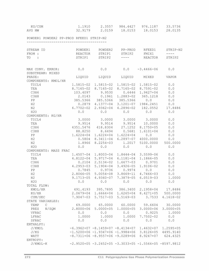
272 C11 Polypropylene Gas Phase Polymerization Processes
KG/CUM 1.1910 2.3557 984.4427 976.1187 33.5736 AVG MW 32.9179 2.0159 18.0153 18.0153 28.0135 POWDER1 POWDER2 PP-PROD RFEED1 STRIP-N2 --------------------------------------- STREAM ID POWDER1 POWDER2 PP-PROD RFEED1 STRIP-N2 FROM : REACTOR STRIP1 STRIP2 FMIX1 ---- TO : STRIP1 STRIP2 ---- REACTOR STRIP2 MAX CONV. ERROR: 0.0 0.0 0.0 -3.4466-06 0.0 SUBSTREAM: MIXED PHASE: LIQUID LIQUID LIQUID MIXED VAPOR COMPONENTS: KMOL/HR TICL4 1.5815-02 1.5815-02 1.5815-02 1.5815-02 0.0 TEA 8.7165-02 8.7165-02 8.7165-02 8.7591-02 0.0 C3H6 103.4097 9.9530 0.6446 1.9427+04 0.0 C3H8 2.0143 0.1961 1.2883-02 365.1218 0.0 PP 385.5366 385.5366 385.5366 0.0 0.0 H2 0.2879 4.1377-04 3.1201-07 1984.2451 0.0 N2 6.7702-02 2.9362-04 4.2896-02 182.0552 17.8486 H2O 0.0 0.0 0.0 0.0 0.0 COMPONENTS: KG/HR TICL4 3.0000 3.0000 3.0000 3.0000 0.0 TEA 9.9514 9.9514 9.9514 10.0000 0.0 C3H6 4351.5476 418.8304 27.1252 8.1750+05 0.0 C3H8 88.8250 8.6494 0.5681 1.6101+04 0.0 PP 1.6224+04 1.6224+04 1.6224+04 0.0 0.0 H2 0.5804 8.3411-04 6.2897-07 4000.0000 0.0 N2 1.8966 8.2254-03 1.2017 5100.0000 500.0000 H2O 0.0 0.0 0.0 0.0 0.0 COMPONENTS: MASS FRAC TICL4 1.4507-04 1.8003-04 1.8444-04 3.5599-06 0.0 TEA 4.8122-04 5.9717-04 6.1181-04 1.1866-05 0.0 C3H6 0.2104 2.5134-02 1.6677-03 0.9701 0.0 C3H8 4.2953-03 5.1904-04 3.4926-05 1.9106-02 0.0 PP 0.7845 0.9736 0.9974 0.0 0.0 H2 2.8066-05 5.0054-08 3.8669-11 4.7466-03 0.0 N2 9.1713-05 4.9360-07 7.3879-05 6.0519-03 1.0000 H2O 0.0 0.0 0.0 0.0 0.0 TOTAL FLOW: KMOL/HR 491.4193 395.7895 386.3400 2.1958+04 17.8486 KG/HR 2.0679+04 1.6664+04 1.6265+04 8.4271+05 500.0000 CUM/SEC 7.9047-03 5.7517-03 5.5169-03 3.7533 4.1618-02 STATE VARIABLES: TEMP C 69.0000 65.0000 60.0000 59.6604 30.0000 PRES N/SQM 2.8000+06 5.0000+05 1.0000+05 3.0000+06 3.0000+05 VFRAC 0.0 0.0 0.0 0.9225 1.0000 LFRAC 1.0000 1.0000 1.0000 7.7502-02 0.0 SFRAC 0.0 0.0 0.0 0.0 0.0 ENTHALPY: J/KMOL -6.3962+07 -8.1459+07 -8.4134+07 1.4632+07 1.2595+05 J/KG -1.5200+06 -1.9347+06 -1.9984+06 3.8126+05 4495.9140 WATT -8.7311+06 -8.9557+06 -9.0289+06 8.9247+07 624.4325 ENTROPY: J/KMOL-K -2.9520+05 -3.2452+05 -3.3033+05 -1.5564+05 -8597.9812
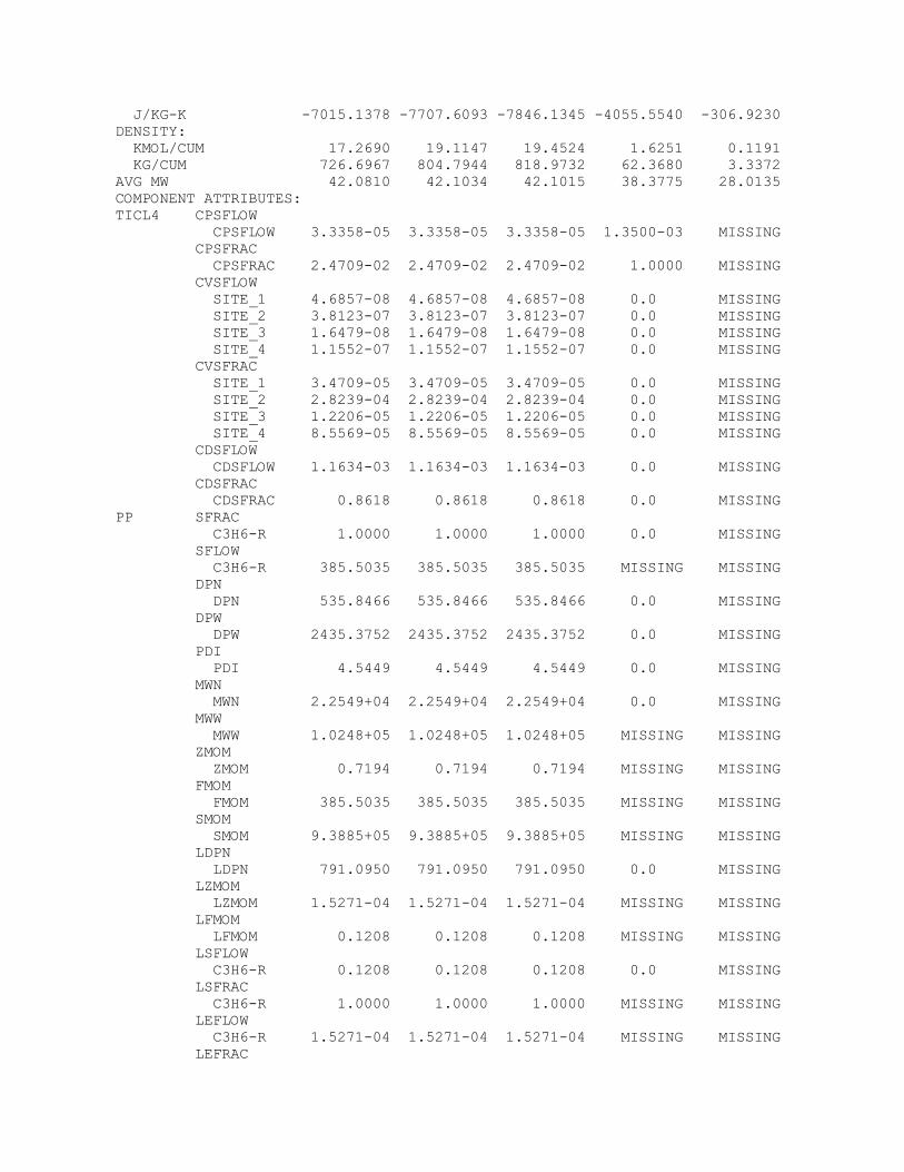
J/KG-K -7015.1378 -7707.6093 -7846.1345 -4055.5540 -306.9230 DENSITY: KMOL/CUM 17.2690 19.1147 19.4524 1.6251 0.1191 KG/CUM 726.6967 804.7944 818.9732 62.3680 3.3372 AVG MW 42.0810 42.1034 42.1015 38.3775 28.0135 COMPONENT ATTRIBUTES: TICL4 CPSFLOW CPSFLOW 3.3358-05 3.3358-05 3.3358-05 1.3500-03 MISSING CPSFRAC CPSFRAC 2.4709-02 2.4709-02 2.4709-02 1.0000 MISSING CVSFLOW SITE_1 4.6857-08 4.6857-08 4.6857-08 0.0 MISSING SITE_2 3.8123-07 3.8123-07 3.8123-07 0.0 MISSING SITE_3 1.6479-08 1.6479-08 1.6479-08 0.0 MISSING SITE_4 1.1552-07 1.1552-07 1.1552-07 0.0 MISSING CVSFRAC SITE_1 3.4709-05 3.4709-05 3.4709-05 0.0 MISSING SITE_2 2.8239-04 2.8239-04 2.8239-04 0.0 MISSING SITE_3 1.2206-05 1.2206-05 1.2206-05 0.0 MISSING SITE_4 8.5569-05 8.5569-05 8.5569-05 0.0 MISSING CDSFLOW CDSFLOW 1.1634-03 1.1634-03 1.1634-03 0.0 MISSING CDSFRAC CDSFRAC 0.8618 0.8618 0.8618 0.0 MISSING PP SFRAC C3H6-R 1.0000 1.0000 1.0000 0.0 MISSING SFLOW C3H6-R 385.5035 385.5035 385.5035 MISSING MISSING DPN DPN 535.8466 535.8466 535.8466 0.0 MISSING DPW DPW 2435.3752 2435.3752 2435.3752 0.0 MISSING PDI PDI 4.5449 4.5449 4.5449 0.0 MISSING MWN MWN 2.2549+04 2.2549+04 2.2549+04 0.0 MISSING MWW MWW 1.0248+05 1.0248+05 1.0248+05 MISSING MISSING ZMOM ZMOM 0.7194 0.7194 0.7194 MISSING MISSING FMOM FMOM 385.5035 385.5035 385.5035 MISSING MISSING SMOM SMOM 9.3885+05 9.3885+05 9.3885+05 MISSING MISSING LDPN LDPN 791.0950 791.0950 791.0950 0.0 MISSING LZMOM LZMOM 1.5271-04 1.5271-04 1.5271-04 MISSING MISSING LFMOM LFMOM 0.1208 0.1208 0.1208 MISSING MISSING LSFLOW C3H6-R 0.1208 0.1208 0.1208 0.0 MISSING LSFRAC C3H6-R 1.0000 1.0000 1.0000 MISSING MISSING LEFLOW C3H6-R 1.5271-04 1.5271-04 1.5271-04 MISSING MISSING LEFRAC
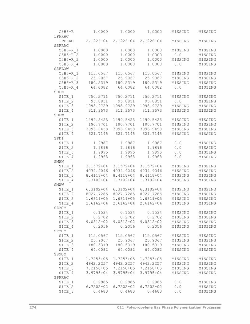
274 C11 Polypropylene Gas Phase Polymerization Processes
C3H6-R 1.0000 1.0000 1.0000 MISSING MISSING LPFRAC LPFRAC 2.1226-04 2.1226-04 2.1226-04 MISSING MISSING SSFRAC C3H6-R_1 1.0000 1.0000 1.0000 MISSING MISSING C3H6-R_2 1.0000 1.0000 1.0000 0.0 MISSING C3H6-R_3 1.0000 1.0000 1.0000 MISSING MISSING C3H6-R_4 1.0000 1.0000 1.0000 0.0 MISSING SSFLOW C3H6-R_1 115.0567 115.0567 115.0567 MISSING MISSING C3H6-R_2 25.9067 25.9067 25.9067 MISSING MISSING C3H6-R_3 180.5319 180.5319 180.5319 MISSING MISSING C3H6-R_4 64.0082 64.0082 64.0082 0.0 MISSING SDPN SITE_1 750.2711 750.2711 750.2711 MISSING MISSING SITE_2 95.8851 95.8851 95.8851 0.0 MISSING SITE_3 1998.9729 1998.9729 1998.9729 MISSING MISSING SITE_4 311.3573 311.3573 311.3573 MISSING MISSING SDPW SITE_1 1499.5423 1499.5423 1499.5423 MISSING MISSING SITE_2 190.7701 190.7701 190.7701 MISSING MISSING SITE_3 3996.9458 3996.9458 3996.9458 MISSING MISSING SITE_4 621.7145 621.7145 621.7145 MISSING MISSING SPDI SITE_1 1.9987 1.9987 1.9987 0.0 MISSING SITE_2 1.9896 1.9896 1.9896 0.0 MISSING SITE_3 1.9995 1.9995 1.9995 0.0 MISSING SITE_4 1.9968 1.9968 1.9968 0.0 MISSING SMWN SITE_1 3.1572+04 3.1572+04 3.1572+04 MISSING MISSING SITE_2 4034.9046 4034.9046 4034.9046 MISSING MISSING SITE_3 8.4118+04 8.4118+04 8.4118+04 MISSING MISSING SITE_4 1.3102+04 1.3102+04 1.3102+04 MISSING MISSING SMWW SITE_1 6.3102+04 6.3102+04 6.3102+04 MISSING MISSING SITE_2 8027.7285 8027.7285 8027.7285 MISSING MISSING SITE_3 1.6819+05 1.6819+05 1.6819+05 MISSING MISSING SITE_4 2.6162+04 2.6162+04 2.6162+04 MISSING MISSING SZMOM SITE_1 0.1534 0.1534 0.1534 MISSING MISSING SITE_2 0.2702 0.2702 0.2702 MISSING MISSING SITE_3 9.0312-02 9.0312-02 9.0312-02 MISSING MISSING SITE_4 0.2056 0.2056 0.2056 MISSING MISSING SFMOM SITE_1 115.0567 115.0567 115.0567 MISSING MISSING SITE_2 25.9067 25.9067 25.9067 MISSING MISSING SITE_3 180.5319 180.5319 180.5319 MISSING MISSING SITE_4 64.0082 64.0082 64.0082 MISSING MISSING SSMOM SITE_1 1.7253+05 1.7253+05 1.7253+05 MISSING MISSING SITE_2 4942.2257 4942.2257 4942.2257 MISSING MISSING SITE_3 7.2158+05 7.2158+05 7.2158+05 MISSING MISSING SITE_4 3.9795+04 3.9795+04 3.9795+04 MISSING MISSING SPFRAC SITE_1 0.2985 0.2985 0.2985 0.0 MISSING SITE_2 6.7202-02 6.7202-02 6.7202-02 0.0 MISSING SITE_3 0.4683 0.4683 0.4683 0.0 MISSING
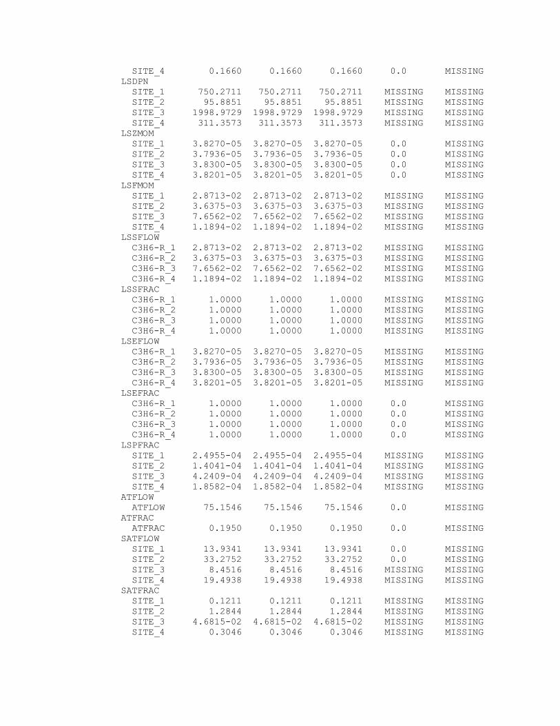
SITE_4 0.1660 0.1660 0.1660 0.0 MISSING LSDPN SITE_1 750.2711 750.2711 750.2711 MISSING MISSING SITE_2 95.8851 95.8851 95.8851 MISSING MISSING SITE_3 1998.9729 1998.9729 1998.9729 MISSING MISSING SITE_4 311.3573 311.3573 311.3573 MISSING MISSING LSZMOM SITE_1 3.8270-05 3.8270-05 3.8270-05 0.0 MISSING SITE_2 3.7936-05 3.7936-05 3.7936-05 0.0 MISSING SITE_3 3.8300-05 3.8300-05 3.8300-05 0.0 MISSING SITE_4 3.8201-05 3.8201-05 3.8201-05 0.0 MISSING LSFMOM SITE_1 2.8713-02 2.8713-02 2.8713-02 MISSING MISSING SITE_2 3.6375-03 3.6375-03 3.6375-03 MISSING MISSING SITE_3 7.6562-02 7.6562-02 7.6562-02 MISSING MISSING SITE_4 1.1894-02 1.1894-02 1.1894-02 MISSING MISSING LSSFLOW C3H6-R_1 2.8713-02 2.8713-02 2.8713-02 MISSING MISSING C3H6-R_2 3.6375-03 3.6375-03 3.6375-03 MISSING MISSING C3H6-R_3 7.6562-02 7.6562-02 7.6562-02 MISSING MISSING C3H6-R_4 1.1894-02 1.1894-02 1.1894-02 MISSING MISSING LSSFRAC C3H6-R_1 1.0000 1.0000 1.0000 MISSING MISSING C3H6-R_2 1.0000 1.0000 1.0000 MISSING MISSING C3H6-R_3 1.0000 1.0000 1.0000 MISSING MISSING C3H6-R_4 1.0000 1.0000 1.0000 MISSING MISSING LSEFLOW C3H6-R_1 3.8270-05 3.8270-05 3.8270-05 MISSING MISSING C3H6-R_2 3.7936-05 3.7936-05 3.7936-05 MISSING MISSING C3H6-R_3 3.8300-05 3.8300-05 3.8300-05 MISSING MISSING C3H6-R_4 3.8201-05 3.8201-05 3.8201-05 MISSING MISSING LSEFRAC C3H6-R_1 1.0000 1.0000 1.0000 0.0 MISSING C3H6-R_2 1.0000 1.0000 1.0000 0.0 MISSING C3H6-R_3 1.0000 1.0000 1.0000 0.0 MISSING C3H6-R_4 1.0000 1.0000 1.0000 0.0 MISSING LSPFRAC SITE_1 2.4955-04 2.4955-04 2.4955-04 MISSING MISSING SITE_2 1.4041-04 1.4041-04 1.4041-04 MISSING MISSING SITE_3 4.2409-04 4.2409-04 4.2409-04 MISSING MISSING SITE_4 1.8582-04 1.8582-04 1.8582-04 MISSING MISSING ATFLOW ATFLOW 75.1546 75.1546 75.1546 0.0 MISSING ATFRAC ATFRAC 0.1950 0.1950 0.1950 0.0 MISSING SATFLOW SITE_1 13.9341 13.9341 13.9341 0.0 MISSING SITE_2 33.2752 33.2752 33.2752 0.0 MISSING SITE_3 8.4516 8.4516 8.4516 MISSING MISSING SITE_4 19.4938 19.4938 19.4938 MISSING MISSING SATFRAC SITE_1 0.1211 0.1211 0.1211 MISSING MISSING SITE_2 1.2844 1.2844 1.2844 MISSING MISSING SITE_3 4.6815-02 4.6815-02 4.6815-02 MISSING MISSING SITE_4 0.3046 0.3046 0.3046 MISSING MISSING
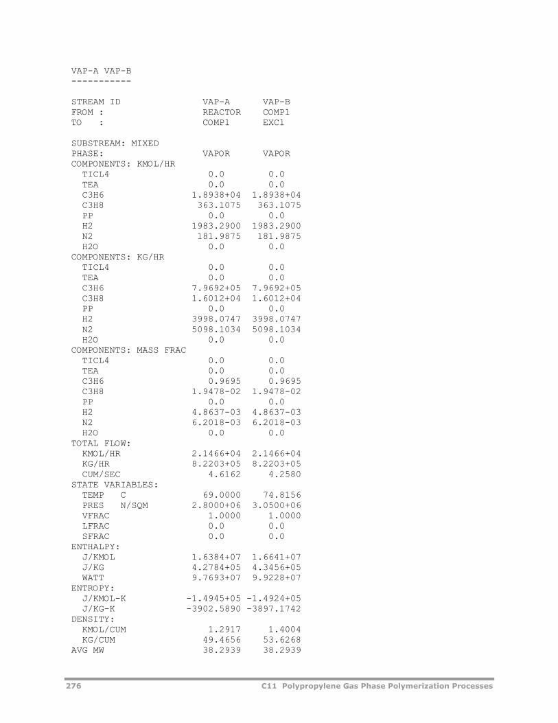
276 C11 Polypropylene Gas Phase Polymerization Processes
VAP-A VAP-B ----------- STREAM ID VAP-A VAP-B FROM : REACTOR COMP1 TO : COMP1 EXC1 SUBSTREAM: MIXED PHASE: VAPOR VAPOR COMPONENTS: KMOL/HR TICL4 0.0 0.0 TEA 0.0 0.0 C3H6 1.8938+04 1.8938+04 C3H8 363.1075 363.1075 PP 0.0 0.0 H2 1983.2900 1983.2900 N2 181.9875 181.9875 H2O 0.0 0.0 COMPONENTS: KG/HR TICL4 0.0 0.0 TEA 0.0 0.0 C3H6 7.9692+05 7.9692+05 C3H8 1.6012+04 1.6012+04 PP 0.0 0.0 H2 3998.0747 3998.0747 N2 5098.1034 5098.1034 H2O 0.0 0.0 COMPONENTS: MASS FRAC TICL4 0.0 0.0 TEA 0.0 0.0 C3H6 0.9695 0.9695 C3H8 1.9478-02 1.9478-02 PP 0.0 0.0 H2 4.8637-03 4.8637-03 N2 6.2018-03 6.2018-03 H2O 0.0 0.0 TOTAL FLOW: KMOL/HR 2.1466+04 2.1466+04 KG/HR 8.2203+05 8.2203+05 CUM/SEC 4.6162 4.2580 STATE VARIABLES: TEMP C 69.0000 74.8156 PRES N/SQM 2.8000+06 3.0500+06 VFRAC 1.0000 1.0000 LFRAC 0.0 0.0 SFRAC 0.0 0.0 ENTHALPY: J/KMOL 1.6384+07 1.6641+07 J/KG 4.2784+05 4.3456+05 WATT 9.7693+07 9.9228+07 ENTROPY: J/KMOL-K -1.4945+05 -1.4924+05 J/KG-K -3902.5890 -3897.1742 DENSITY: KMOL/CUM 1.2917 1.4004 KG/CUM 49.4656 53.6268 AVG MW 38.2939 38.2939
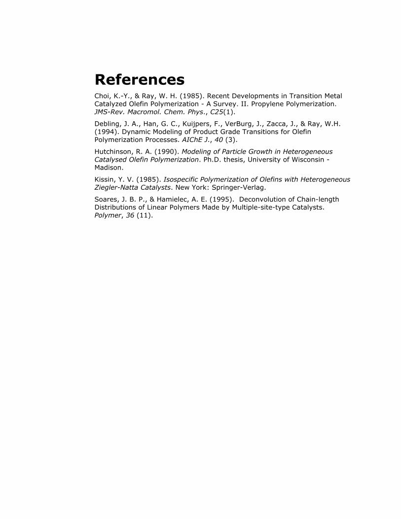
References Choi, K.-Y., & Ray, W. H. (1985). Recent Developments in Transition Metal Catalyzed Olefin Polymerization - A Survey. II. Propylene Polymerization. JMS-Rev. Macromol. Chem. Phys., C25(1).
Debling, J. A., Han, G. C., Kuijpers, F., VerBurg, J., Zacca, J., & Ray, W.H. (1994). Dynamic Modeling of Product Grade Transitions for Olefin Polymerization Processes. AIChE J., 40 (3).
Hutchinson, R. A. (1990). Modeling of Particle Growth in Heterogeneous Catalysed Olefin Polymerization. Ph.D. thesis, University of Wisconsin - Madison.
Kissin, Y. V. (1985). Isospecific Polymerization of Olefins with Heterogeneous Ziegler-Natta Catalysts. New York: Springer-Verlag.
Soares, J. B. P., & Hamielec, A. E. (1995). Deconvolution of Chain-length Distributions of Linear Polymers Made by Multiple-site-type Catalysts. Polymer, 36 (11).
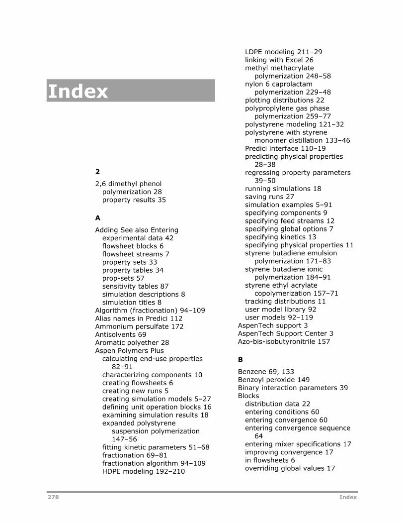
278 Index
Index
2
2,6 dimethyl phenol polymerization 28 property results 35
A
Adding See also Entering experimental data 42 flowsheet blocks 6 flowsheet streams 7 property sets 33 property tables 34 prop-sets 57 sensitivity tables 87 simulation descriptions 8 simulation titles 8
Algorithm (fractionation) 94–109 Alias names in Predici 112 Ammonium persulfate 172 Antisolvents 69 Aromatic polyether 28 Aspen Polymers Plus
calculating end-use properties 82–91
characterizing components 10 creating flowsheets 6 creating new runs 5 creating simulation models 5–27 defining unit operation blocks 16 examining simulation results 18 expanded polystyrene
suspension polymerization 147–56
fitting kinetic parameters 51–68 fractionation 69–81 fractionation algorithm 94–109 HDPE modeling 192–210
LDPE modeling 211–29 linking with Excel 26 methyl methacrylate
polymerization 248–58 nylon 6 caprolactam
polymerization 229–48 plotting distributions 22 polyproplylene gas phase
polymerization 259–77 polystyrene modeling 121–32 polystyrene with styrene
monomer distillation 133–46 Predici interface 110–19 predicting physical properties
28–38 regressing property parameters
39–50 running simulations 18 saving runs 27 simulation examples 5–91 specifying components 9 specifying feed streams 12 specifying global options 7 specifying kinetics 13 specifying physical properties 11 styrene butadiene emulsion
polymerization 171–83 styrene butadiene ionic
polymerization 184–91 styrene ethyl acrylate
copolymerization 157–71 tracking distributions 11 user model library 92 user models 92–119
AspenTech support 3 AspenTech Support Center 3 Azo-bis-isobutyronitrile 157
B
Benzene 69, 133 Benzoyl peroxide 149 Binary interaction parameters 39 Blocks
distribution data 22 entering conditions 60 entering convergence 60 entering convergence sequence
64 entering mixer specifications 17 improving convergence 17 in flowsheets 6 overriding global values 17
renaming 7 specifying 16
Blowing agents 148 Building
process flowsheets 6 simulation models 5–27
Bulk polymerization 121–32 Butadiene
styrene emulsion copolymerization 171–83
styrene ionic polymerization 184–91
C
Calculating end-use properties 82–91 properties 76
Caprolactam conversion 244 example flowsheet 231 example input summary 239 example kinetics 233 example process conditions 232 example process studies 239 example results 244 example stream summary 245 extraction value results 244 Mn results 244 nylon 6 polymerization 229–48 step-growth polymerization 230
Catalysts for Ziegler-Natta 192 Chain length distribution
results (Predici interface) 115 results (SBR) 182
Chain transfer agents dodecyl mercaptan 123 ethyl benzene 123, 133 hydrogen 193 tertiary dodecyl mercaptane 172
Characterizing oligomers 10 polymers 10 segments 10 site-based species 10
Components entering pure component
parameters 56 mapping from Predici 111, 113 polydispersity 94 predicting properties for 28–38 specifying 9, 30
Convergence
for blocks 60, 64 improving 17
Creating alias file for Predici 112 data sets 61 flowsheets 6 new runs 5 property sets 33 property tables 34 sensitivity tables 87 simulation models 5–27
Crystallinity 33 Custom
MWD data 103 Custom property parameters 11 customer support 3
D
Data experimental 42 fitting 51–68 regression 39–50 sets 61
Data fit folder 61 specifying regression cases 63
Data regression entering experimental data 42 example for property parameters
39–50 input summary 48 results 65 specifying 61 specifying regression cases 45
Defining mass fraction crystallinity 33 molecular structure 32 oligomers 10 polymers 10 segments 10 site-based species 10
Density predicting 28 results for 2,6 dimethyl phenol
35 Descriptions for simulations 8 Distillation of polystyrene 133–46 Distributions
for flowsheets 22 for reactors 22 for streams 22 linking with Excel 26
280 Index
live plots 23 plots for multiple simulations 24 plotting 22 tables 22 tracking 11
Di-tert-butyl peroxide 123 Dodecyl mercaptan 123 DRS See Data regression
E
e-bulletins 3 Editing reactions 13 Emulsifiers 172 Emulsion polymerization of styrene
butadiene 171–83 End-use properties
calculating 82–91 input summary 89
Entering See also Specifying, See also Adding
block conditions 60 block convergence 60 block convergence sequence 64 experimental data 42 prop-sets 57 pseudo-components for
fractionation model 95 pure component parameters 56 simulation descriptions 8 simulation titles 8 stream conditions 60
EPS See Expanded polystyrene Equations of state
fitting parameters 39–50 Sanchez-Lacombe 39
Ethanol 69 Ethyl acetate polymerization 248–
58 Ethyl acrylate copolymerization
157–71 Ethyl benzene 123, 133 Ethylene
conversion 200 HDPE polymerization 192–210 LDPE polymerization 211–29
Ethylene-polyethylene 39 Examples
calculating end-use properties 82–91
expanded polystyrene suspension polymerization 147–56
fitting kinetic parameters 51–68 fractionating oligomers 69–81 HDPE polymerization 192–210 LDPE polymerization 211–29 methyl methacrylate
polymerization 248–58 nylon 6 caprolactam
polymerization 229–48 polymer fractionation algorithm
96, 103 polypropylene gas phase
polymerization 259–77 polystyrene bulk polymerization
121–32 polystyrene with styrene
monomer distillation 133–46 Predici interface 114 predicting physical properties
28–38 regressing property parameters
39–50 styrene butadiene emulsion
copolymerization 171–83 styrene butadiene ionic
polymerization 184–91 styrene ethyl acrylate
copolymerization 157–71 Excel
linking 26 Expanded polystyrene
conversion effects 154 example flowsheet 148 example input summary 151 example kinetics 150 example process conditions 149 example process studies 151 example results 154 free-radical polymerization 147 number average molecular
weight 155 polymerization 147–56
Experimental data 42
F
Feed flow rate effect on ethylene conversion
200 effect on extraction value 244 effect on hydrogen concentration
202 effect on melt index 203 effect on Mn 201, 244
effect on Mw 202 effect on number average
molecular weight 128 effect on polydispersity 129, 203 effect on recycle rate 130 effect on styrene conversion 128 effect on weight average
molecular weight 129 Feed streams specification 12 Files
for polymer fractionation 95 Fitting
input summary example 66 kinetic parameters 51–68 mixture parameters 39–50
Flash algorithm (Polymix) 94–109
Flory-Huggins model 69 Flow rate See Feed flow rate Flowsheets
creating 6 distribution data 22 placing blocks 6 placing streams 7 renaming blocks 7 renaming streams 7
Fortran subroutines 82, 89 Fractionation
example 69–81 input summary 79
Fractionation algorithm creating working directory 95 entering pseudo-components 95 files delivered 95 input summary (PolFrac1) 97 input summary (PolFrac2) 106 installing model 95 opening model 95 phase analysis results 105 PolFrac1 example 96 PolFrac2 example 103 restrictions 94–109 running model 96 separation results 96 stream report (PolFrac1) 100 stream report (PolFrac2) 108 User2 model 94–109
Free-radical polymerization of ethylene 211–29 of expanded polystyrene 147–56 of methyl methacrylate 248–58 of polystyrene 121–32 of styrene butadiene 171–83
of styrene ethyl acrylate 157–71
G
Gas-phase polymerization 259–77 Gel effect specification 15 Global options
defining unit-sets 8 overriding values 17 report options 9 specifying 7
Group contribution method 28
H
HDPE conversion results 200 example flowsheet 193 example input summary 195 example kinetics 194 example model 192–210 example process conditions 193 example process studies 194 example results 200 hydrogen concentration results
202, 204 melt index results 203 Mn results 201 molecular weight distribution 205 Mw results 202 polydispersity results 203 stream summary 205
Heat capacity predicting 28 results for 2,6 dimethyl phenol
35 help desk 3 High-density polyethylene See
HDPE Hydrogen 193 Hydrogen concentration 202, 204
I
Inhibitors 136 Initiation
results 65 thermal 121–32
Initiators ammonium persulfate 172 benzoyl peroxide 149 decomposition vs reactor length
220 methyl peroxide 51
282 Index
Input summary for data regression example 48 for end-use properties example
89 for expanded polystyrene
polymerization 151 for fitting kinetic parameters
example 66 for HDPE polymerization 195 for LDPE polymerization 215 for methyl methacrylate
polymerization 251 for nylon 6 caprolactam
polymerization 239 for oligomer fractionation 79 for polymer fractionation
(PolFrac1) 97 for polymer fractionation
(PolFrac2) 106 for polypropylene polymerization
264 for polystyrene bulk
polymerization 124 for polystyrene with styrene
monomer distillation 136 for Predici interface 116 for predicting physical properties
example 37 for styrene ethyl acrylate
copolymerization 163 for styrene-butadiene emulsion
copolymerization 177 for styrene-butadiene ionic
polymerization 187 Installing
polymer fractionation model 95 user model library 92
Intrinsic viscosity 82 Ionic polymerization
of styrene butadiene 184–91
K
Kinetics fitting parameters 51–68 modifying reactions 13 specifying 13 specifying gel effect 15
L
LDPE coolant temperature profiles 220
DPn and DPw vs reactor length 219
ethylene mole fraction 221 example flowsheet 211 example input summary 215 example kinetics 214 example model 211–29 example process conditions 213 example process studies 215 example results 219 free-radical polymerization 211 initiator decomposition vs reactor
length 220 reactant temperature profiles
220 reactor temperature profiles 221 stream summary 222
Linking Aspen Polymers Plus with Excel
26 Poymers Plus with Predici 111
Live plots 23 Low-density polyethylene See LDPE
M
Mapping Predici alias names 113 Predici components 111
Mass fraction crystallinity 33 Melt index 82 Methanol 51 Methyl methacrylate
example flowsheet 249 example input summary 251 example kinetics 251 example process conditions 250 example process studies 251 example results 253 flow vs time 253 free-radical polymerization 249 heat duty 256 MWn vs temperature 255 MWw vs temperature 255 number-average molecular
weight vs time 254 polydispersity 256 polymerization in ethyl acetate
248–58 reaction time for monomer
conversion 254 Methyl peroxide 51 Mixers 17
Mixtures ethylene-polyethylene 39 fitting paramters 39–50
Molecular structure 32 Molecular weight distribution
custom data 103 HDPE example 205 in polymer fractionation 94
MWD See Molecular weight distribution
N
n-hexane 193 n-pentane 148 Nylon 6
caprolactam conversion 244 caprolactam polymerization 229–
48 example flowsheet 231 example input summary 239 example kinetics 233 example process conditions 232 example process studies 239 example results 244 example stream summary 245 extraction value results 244 Mn results 244 step-growth polymerization 230
O
OLE linking 26 Oligomers
characterizing 10 fractionation example 69–81
Opening Aspen Polymers Plus 5 Aspen Polymers Plus-Predici
model 110 fractionation model 95 user models 92
P
Parameters binary interaction 39 entering pure component 56 fitting kinetic 51–68 fitting mixture 39–50 Flory-Huggins 69 for polypropylene example 263 regression for styrene ethyl
acrylate example 160
specifying 46 specifying binary interaction 75 specifying custom 11
Physical properties example input summary 37 predicting parameters 28–38 regressing parameters 39–50
Plotting distributions 22 live plots 23 manually 25 multiple simulations 24
Poly(phenylene oxide) 28 Polydispersity 69, 94 Polyethylene
HDPE polymerization 192–210 intrinsic viscosity 82 LDPE polymerization 211–29 melt index 82 zero-shear viscosity 82 Ziegler-Natta polymerization 192
Polymer fractionation See Fractionation algorithm
Polymerization bulk 121–32 emulsion 171–83 gas-phase 259–77 ionic 184–91 of expanded polystyrene 147–56 of HDPE 192–210 of LDPE 211–29 of methyl methacrylate 248–58 of nylon 6 caprolactam 229–48 of polypropylene 259–77 of polystyrene by thermal
initiation 121–32 of styrene butadiene 171–83,
184–91 of styrene ethyl acrylate 157–71 solution 192–210, 248–58 suspension 147–56, 259–77
Polymers 2,6 dimethyl phenol 28 aromatic polyether 28 characterizing 10 end-use properties 82–91 ethylene-polyethylene 39 fractionation algorithm 94–109 fractionation example 69–81 poly(phenylene oxide) 28 polystyrene 69 predicting formation during
styrene distillation 133–46
284 Index
specifying mass fraction drystallinity 33
vinyl acetate 51 Polymethyl methacrylate See
Methyl methacrylate PolyMix 94 Polyolefin 211 Polyolefins 39 Polypropylene
example flowsheet 260 example input summary 264 example kinetics 263 example parameters 263 example process conditions 261 example results 269 example stream summary 269 gas phase polymerization 259–
77 process types 259
Polystyrene See also Expanded polystyrene
bulk polymerization 121–32 example flowsheet 121 example input summary 124 example kinetics 123 example process conditions 122 example process studies 124 example results 128 example stream summary 130 fractionation 69 fractionation results 78 free-radical polymerization 121 number average molecular
weight 128 polydispersity 69, 129 recycle rate 130 styrene monomer distillation
133–46 thermal initiation example 96 weight average molecular weight
129 Polystyrene distillation
example flowsheet 133 example input summary 136 example kinetics 136 example process conditions 134 example results 141 example stream summary 143 inhibitor 136 polymer production results 142 profitability results 142 sensitivity study 141
Predici interface
creating alias file 112 example 114 input summary 116 linking with Aspen Polymers Plus
111 mapping component names 113 mapping components 111 opening model 110 running model 114 specifying alias names 112 specifying stream flash 113 stream report 118 using 110–19
Process models See Simulations Propagation results 65 Properties
creating property sets 33 creating property tables 34 end-use 82–91 estimating 29 predicting density 28 predicting heat capacity 28 predicting parameters 28–38 predicting thermal conducivity 28 regressing parameters 39–50 specifying calculations 76 specifying custom parameters 11 specifying parameters 46, 75
Property analysis 29 methods 11, 42 parameters 46 sets 33 tables 34
Prop-sets defining 57 fortran subroutines 82
Pseudo-component approach 69 Pseudo-components 95 Pure components
parameters 56 predicting properties for 28–38
R
Rate constants example input screen 14 for styrene-butadiene emulsion
example 175 Reactions
modifying 13 rate constants 14
Reactor distribution data 22
Regression cases 45, 63 for styrene ethyl acrylate
example 160 Renaming
flowsheet blocks 7 flowsheet streams 7
Reports defining options 9 displaying a prop-set 57
Results chain length distribution (Predici
interface) 115 chain length distribution (SBR)
182 for expanded polystyrene
polymerization 154 for HDPE polymerization 200 for initiation 65 for LDPE polymerization 219 for methyl methacrylate
polymerization 253 for nylon 6 caprolactam
polymerization 244 for PolFrac1 example 96 for PolFrac2 example 105 for polymer density 35 for polymer heat capacity 35 for polymer thermal conductivity
35 for polypropylene polymerization
269 for polystyrene bulk
polymerization 128 for polystyrene with styrene
distillation 141 for propagation 65 for styrene ethyl acrylate
copolymerization 167 for styrene-butadiene emulsion
copolymerization 180 for styrene-butadiene ionic
polymerization 189 fractionation of polystyrene 78 plotting 22 reviewing 18 saving 27
Reviewing distribution tables 22 results 18
Run types data regression 40 flowsheet 6
property analysis 29 Running
Aspen Polymers Plus 5 fractionation model 96 Polymers-Plus-Predici model 114
S
Sanchez-Lacombe 39 Saving 27 SBR See Styrene butadiene Segments
characterizing 10 defining molecular structure 32
Sensitivity tables 87 Setup options
adding descriptions 8 adding titles 8 defining unit-sets 8 report options 9 specifying 7 specifying time limits 9
Simulations calculating end-use properties
82–91 creating flowsheets 6 creating models 5–27 creating new runs 5 defining report options 9 defining unit-sets 8 entering descriptions for 8 entering time limits 9 entering titles for 8 examples 5–91 expanded polystyrene
suspension polymerization 147–56
fitting kinetic parameters 51–68 fractionating oligomers 69–81 HDPE polymerization 192–210 LDPE polymerization 211–29 methyl methacrylate
polymerization 248–58 nylon 6 caprolactam
polymerization 229–48 plotting multiple 24 polymer fractionation algorithm
94–109 polypropylene gas phase
polymerization 259–77 polystyrene bulk polymerization
121–32
286 Index
polystyrene with styrene monomer distillation 133–46
Predici interface 110–19 predicting physical properties
28–38 regressing property parameters
39–50 results 18 running 18 saving 27 styrene butadiene emulsion
copolymerization 171–83 styrene butadiene ionic
polymerization 184–91 styrene ethyl acrylate
copolymerization 157–71 templates 6 user models 92–119
Site-based species characterization 10
Sodium lauryl sulfate 172 Solution polymerization 192–210,
248–58 Solvents
benzene 69, 133 methanol 51 n-hexane 193 toluene 133
Species characterization 10 Specifying See also Entering
alias names in Predici 112 binary interaction parameters 75 block conditions 60 block convergence 60 block convergence sequence 64 components 9, 30 custom property parameters 11 data regression 61 data regression cases 45, 63 data sets 61 distributions 11 feed streams 12 gel effect 15 global options 7 kinetics 13 mass fraction crystallinity 33 mixers 17 molecular structure 32 physical property methods 11 property calculations 76 property methods 42 property parameters 46 prop-sets 57
pseudo-components for fractionation model 95
report options 9, 57 setup options 7 simulation time limits 9 stream conditions 60 stream flash in Predici interface
113 unit operation blocks 16 unit-sets 8
Starting Aspen Polymers Plus 5 simulation runs 18 user models 92
Step-growth polymerization of caprolactam 229–48
Stream report See Stream summary
Stream summary for Predici interface 118 for HDPE polymerization 205 for LDPE polymerization 222 for Nylon 6 caprolactam
polymerization 245 for polymer fractionation
example (PolFrac1) 100 for polymer fractionation
example (PolFrac2) 108 for polypropylene polymerization
269 for polystyrene bulk
polymerization 130 for polystyrene with styrene
distillation 143 Streams
distribution data 22 entering conditions 60 in flowsheets 7 renaming 7 report options 57 specifying 12 specifying flash in Predici
interface 113 Styrene
bulk polymerization 121–32 butadiene emulsion
copolymerization 171–83 butadiene ionic polymerization
184–91 conversion results 128 ethyl acrylate copolymerization
157–71 example flowsheet 121
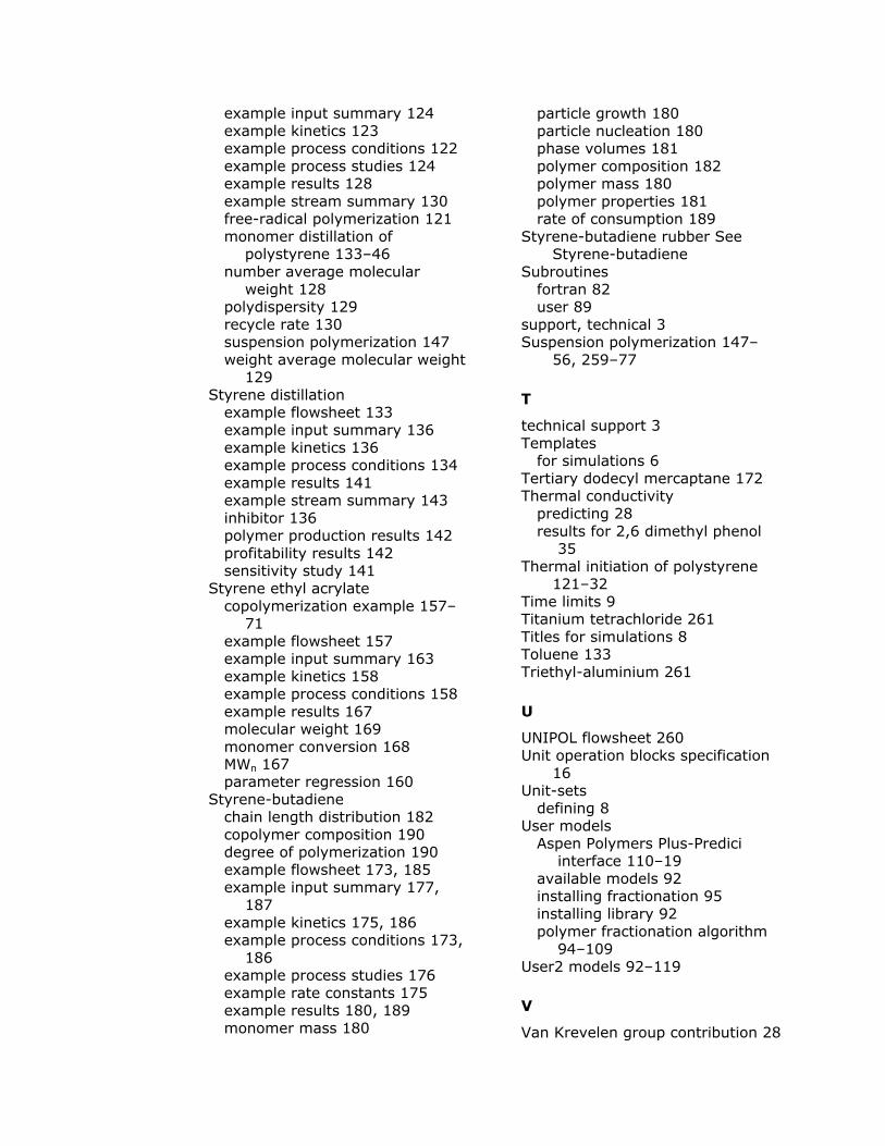
example input summary 124 example kinetics 123 example process conditions 122 example process studies 124 example results 128 example stream summary 130 free-radical polymerization 121 monomer distillation of
polystyrene 133–46 number average molecular
weight 128 polydispersity 129 recycle rate 130 suspension polymerization 147 weight average molecular weight
129 Styrene distillation
example flowsheet 133 example input summary 136 example kinetics 136 example process conditions 134 example results 141 example stream summary 143 inhibitor 136 polymer production results 142 profitability results 142 sensitivity study 141
Styrene ethyl acrylate copolymerization example 157–
71 example flowsheet 157 example input summary 163 example kinetics 158 example process conditions 158 example results 167 molecular weight 169 monomer conversion 168 MWn 167 parameter regression 160
Styrene-butadiene chain length distribution 182 copolymer composition 190 degree of polymerization 190 example flowsheet 173, 185 example input summary 177,
187 example kinetics 175, 186 example process conditions 173,
186 example process studies 176 example rate constants 175 example results 180, 189 monomer mass 180
particle growth 180 particle nucleation 180 phase volumes 181 polymer composition 182 polymer mass 180 polymer properties 181 rate of consumption 189
Styrene-butadiene rubber See Styrene-butadiene
Subroutines fortran 82 user 89
support, technical 3 Suspension polymerization 147–
56, 259–77
T
technical support 3 Templates
for simulations 6 Tertiary dodecyl mercaptane 172 Thermal conductivity
predicting 28 results for 2,6 dimethyl phenol
35 Thermal initiation of polystyrene
121–32 Time limits 9 Titanium tetrachloride 261 Titles for simulations 8 Toluene 133 Triethyl-aluminium 261
U
UNIPOL flowsheet 260 Unit operation blocks specification
16 Unit-sets
defining 8 User models
Aspen Polymers Plus-Predici interface 110–19
available models 92 installing fractionation 95 installing library 92 polymer fractionation algorithm
94–109 User2 models 92–119
V
Van Krevelen group contribution 28
288 Index
Vapor-liquid equilibrium 39 Vinyl acetate 51 Viscosity
intrinsic 82 zero-shear 82
VK column 230
W
web site, technical support 3
Z
Zero-shear viscosity 82 Ziegler-Natta catalysts 192 Ziegler-Natta polymerization
of ethylene 192–210 of polypropylene 259–77


![Îb Aspen Plus ]](https://img.pdfslide.us/doc/110x75/624b1b2716239c1df5539681/b-aspen-plus-.jpg)