Aspects of Vertex Algebras in Geometry and Physics

by

Wolfgang Riedler

A thesis submitted in partial fulfillment of the requirements for the degree of

Doctor of Philosophy

in

Mathematics

Department of Mathematical and Statistical Sciences

University of Alberta

c© Wolfgang Riedler, 2019

Abstract

This thesis studies various aspects of the theory of vertex algebras.

It has been shown that the moonshine module for Conway’s group C0 has

close ties to the equivariant elliptic genera of sigma models with a K3 surface

as target space. This is taken as a motivation to investigate conditions under

which a self-dual vertex operator superalgebra and the bulk Hilbert space of a

superconformal field theory may be identified. To that end a classification of

self-dual vertex operator superalgebras with central charge less than or equal

to 12 is given and several examples of how these vertex algebras can be related

to bulk superconformal field theories are provided. This includes field theories

which arise from sigma models where the target space is a torus or a K3

surface.

Following this, we study orbifolds and cosets of the small N = 4 super-

conformal algebra. Minimal strong generators for generic and specific levels

are found and as a corollary we obtain the vertex algebra of global sections

of the chiral de Rham complex on any complex Enriques surface. The com-

mutant Com(V `(sl2), V `+1(sl2) ⊗W−5/2(sl4, frect)) is identified with orbifolds

of cosets of the small N = 4 superconformal algebra which, in addition, can

be identified with Grassmannian cosets and principalW-algebras of type A at

special levels. We conclude by proving a new level-rank duality which includes

Grassmannian supercosets.

Furthermore, we provide a constructive proof of existence of an embedding

of the Odake vertex algebra into a lattice vertex algebra in any dimension.

ii

In addition, we show that the elliptic genus of this family of lattice vertex

algebras at hand is non-vanishing if and only if the dimension does not equal

1.

Finally, we investigate conformal embeddings of maximal affine vertex al-

gebras into rectangular W-algebras at admissible levels. We prove that such

W-algebras are conditionally isomorphic to affine vertex algebras at boundary

admissible levels for cases of type A, B, C and D.

iii

Preface

Chapter 3 is joint work with Thomas Creutzig and John Duncan and has been

published in the Journal of Physics A: Mathematical and Theoretical, Volume

51, Number 3 by IOP Publishing Ltd c©2017. For an online version see

https://doi.org/10.1088/1751-8121/aa9af5

The version printed here is almost identical; exceptions being the correction

of equation 3.3.1, the correction of typographical errors, and a difference in

formatting.

Chapter 4 is joint work with Thomas Creutzig and Andrew Linshaw and

has been submitted for publication. A preprint of the article is available online

https://arxiv.org/abs/1910.02033

Chapter 4 differs to the submitted version as follows: The appendix as it ap-

pears in the article can be found in Appendix A, the format of some equations

and expressions was altered to fit the format of this thesis, and some semantic

and typographical errors have been corrected.

Chapter 5 is joint work with Thomas Creutzig and chapter 6 is joint work

with Thomas Creutzig and Jinwei Yang. An altered and extended version of

each of these chapters will be submitted for publication at a later date. The

versions printed here should not be redistributed by the end-user.

iv

Acknowledgements

Thomas, for your guidance, support, patience, empathy and coffee;

Andy, for sharing some of your insights and discussing ideas;

Michaela and Hannes, for your unwavering support;

Adriana, for making life simpler and more complicated in the best of ways;

Eoin, Jan, and Nitin, for the most welcome distractions;

Thank you.

v

Table of Contents

1 Introduction 1

2 Background 112.1 Vertex algebras . . . . . . . . . . . . . . . . . . . . . . . . . . 112.2 The chiral de Rham complex and invariant theory . . . . . . . 172.3 The quantum Drinfeld-Sokolov reduction and W-algebras . . . 23

3 Self-dual vertex operator superalgebrasand superconformal field theory 273.1 Introduction . . . . . . . . . . . . . . . . . . . . . . . . . . . . 273.2 Background . . . . . . . . . . . . . . . . . . . . . . . . . . . . 32

3.2.1 Vertex Superalgebra . . . . . . . . . . . . . . . . . . . 323.2.2 Modularity . . . . . . . . . . . . . . . . . . . . . . . . 363.2.3 Superconformal Algebras . . . . . . . . . . . . . . . . . 383.2.4 Free Fields . . . . . . . . . . . . . . . . . . . . . . . . . 41

3.3 Self-Dual Vertex Operator Superalgebras . . . . . . . . . . . . 433.4 Superconformal Field Theory . . . . . . . . . . . . . . . . . . 46

3.4.1 Potential Bulk Conformal Field Theory . . . . . . . . . 463.4.2 Potential Bulk Superconformal Field Theory . . . . . . 493.4.3 Superconformal structure . . . . . . . . . . . . . . . . . 52

3.5 Examples . . . . . . . . . . . . . . . . . . . . . . . . . . . . . 553.5.1 Type D Conformal Field Theory . . . . . . . . . . . . . 553.5.2 Type D Superconformal Field Theory . . . . . . . . . . 573.5.3 Type A Superconformal Field Theory . . . . . . . . . . 593.5.4 Gepner Type Superconformal Field Theory . . . . . . . 60

4 Invariant subalgebras of the small N = 4 superconformal alge-bra 654.1 Introduction . . . . . . . . . . . . . . . . . . . . . . . . . . . . 65

4.1.1 Global sections on Enriques surfaces . . . . . . . . . . 664.1.2 Invariant subalgebras of the small N = 4 superconfor-

mal algebra . . . . . . . . . . . . . . . . . . . . . . . . 674.1.3 A new level-rank duality . . . . . . . . . . . . . . . . . 684.1.4 Organization . . . . . . . . . . . . . . . . . . . . . . . 69

4.2 Background . . . . . . . . . . . . . . . . . . . . . . . . . . . . 704.2.1 Vertex Algebras . . . . . . . . . . . . . . . . . . . . . . 704.2.2 Filtrations . . . . . . . . . . . . . . . . . . . . . . . . . 724.2.3 Associative G-modules and orbifolds . . . . . . . . . . 734.2.4 Associated vertex algebra to n4 . . . . . . . . . . . . . 74

4.3 Automorphisms of V k(n4) . . . . . . . . . . . . . . . . . . . . 754.4 Construction of the vertex algebras . . . . . . . . . . . . . . . 76

4.4.1 Construction of V k(n4)U(1). . . . . . . . . . . . . . . . . 76

vi

4.5 Construction of the cyclic orbifold . . . . . . . . . . . . . . . . 834.6 Structure of the vertex algebras . . . . . . . . . . . . . . . . . 874.7 Coset of V k(n4) by its affine subalgebra . . . . . . . . . . . . . 904.8 Level-rank dualities . . . . . . . . . . . . . . . . . . . . . . . . 98

5 Lattice VOAs and vertex algebras of Odake type 1015.1 Embedding VOAs of Odake type . . . . . . . . . . . . . . . . 1025.2 Elliptic genera . . . . . . . . . . . . . . . . . . . . . . . . . . . 111

6 On conformal embeddings of affine VOAs into rectangular W-algebras 1206.1 Background . . . . . . . . . . . . . . . . . . . . . . . . . . . . 1216.2 Obstructions to conformal embeddings of maximal affine sub

vertex algebras . . . . . . . . . . . . . . . . . . . . . . . . . . 1236.2.1 Type A . . . . . . . . . . . . . . . . . . . . . . . . . . 1246.2.2 Type B . . . . . . . . . . . . . . . . . . . . . . . . . . 1266.2.3 Type C . . . . . . . . . . . . . . . . . . . . . . . . . . 1286.2.4 Type D . . . . . . . . . . . . . . . . . . . . . . . . . . 132

7 Conclusion 134

References 137

Appendix A Decoupling relations and singular fields 149A.1 Decoupling relations . . . . . . . . . . . . . . . . . . . . . . . 149A.2 Singular fields in V k(n4)U(1) . . . . . . . . . . . . . . . . . . . 151A.3 Singular fields in V k(n4)Z/2Z . . . . . . . . . . . . . . . . . . . 155

Appendix B Characters of rectangular W-algebras at boundaryprincipal admissible level 157B.1 Type A . . . . . . . . . . . . . . . . . . . . . . . . . . . . . . 157B.2 Type B . . . . . . . . . . . . . . . . . . . . . . . . . . . . . . 159B.3 Type C . . . . . . . . . . . . . . . . . . . . . . . . . . . . . . 165

B.3.1 Principal embedding into son . . . . . . . . . . . . . . 165B.3.2 Principal embedding into sp2n . . . . . . . . . . . . . . 167

B.4 Type D . . . . . . . . . . . . . . . . . . . . . . . . . . . . . . 175

vii

List of Tables

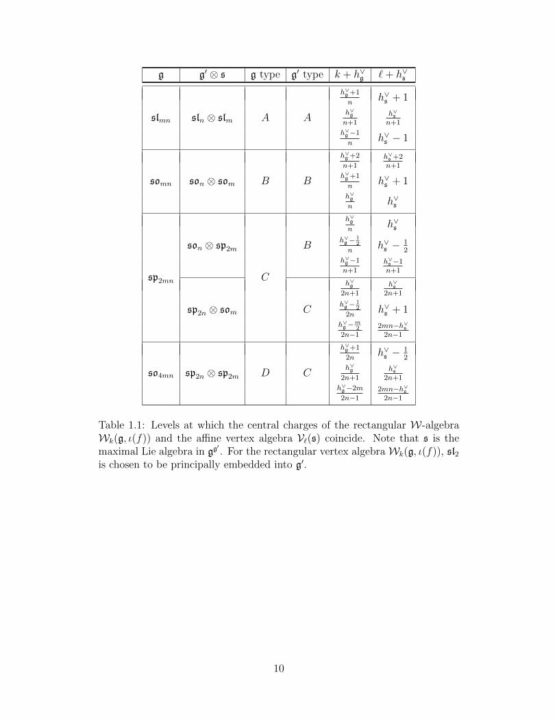
1.1 Levels at which the central charges of the rectangularW-algebraWk(g, ι(f)) and the affine vertex algebra V`(s) coincide. Notethat s is the maximal Lie algebra in gg

′. For the rectangular

vertex algebra Wk(g, ι(f)), sl2 is chosen to be principally em-bedded into g′. . . . . . . . . . . . . . . . . . . . . . . . . . . 10

3.1 Dual Coxeter numbers of simple complex Lie algebras . . . . . 45

5.1 Summary of the preceding examples. The letter χ denotes theEuler characteristic. . . . . . . . . . . . . . . . . . . . . . . . . 115

5.2 Euler Characteristic for the lowest dimensions. . . . . . . . . . 1175.3 Expansions of the conformal field theoretic Hodge-elliptic genus

in lowest dimensions. Setting y = 1 yields the elliptic genusE(τ, u) (cf. Table 5.1). . . . . . . . . . . . . . . . . . . . . . . 119

5.4 Changing all signs in limτ→i∞(zy)c6EHodge(τ, u, v) to be positive

yields the Poincare polynomial (equivalently the Hodge dia-mond). Setting z = y = 1 yields the Euler characteristic. . . . 119

5.5 The Hodge diamond in dimension 3. . . . . . . . . . . . . . . 119

6.1 Examples where s is the maximal Lie algebra in gg′. . . . . . . 121

6.2 Levels at which the central charges of the rectangularW-algebraWk(g, ι(f)) and the affine vertex algebra V`(s) coincide. Notethat s is the maximal Lie algebra in gg

′. For the rectangular

vertex algebra Wk(g, ι(f)), sl2 is chosen to be principally em-bedded into g′. . . . . . . . . . . . . . . . . . . . . . . . . . . 123

viii

Chapter 1

Introduction

Mathematics and physics have enjoyed a fruitful cross-fertilization for nu-

merous decades by now. Amongst the many areas which have ties to both

disciplines is the theory of vertex algebras. This thesis investigates various

aspects of these algebraic objects thereby drawing connections to geometry

and physics. An algebraic object which lies in the intersection of most of the

topics discussed in this thesis is the small N = 4 superconformal extension

of the Virasoro algebra, from here on refered to by n4. A definition of the

associated small N = 4 superconformal vertex algebra Vk(n4) can be taken

to be the minimal W-superalgebra of V−k−1(psl(2|2)). The algebra n4 and its

associated vertex algebra prominently appear in physics, such as string the-

ory on K3 surfaces [ET88b], the AdS/CFT correspondence [Mal99], and as

chiral algebras of certain four-dimensional super Yang-Mills theories [BMR19].

As one amongst many moonshine phenomena, Mathieu moonshine contin-

ues the story that started with Conway and Norton’s monstrous moonshine

conjectures [CN79] which historically paved the way for the definition of ver-

tex algebras. It is here were n4 makes its first appearance: It was observed

in [EOT11] that the elliptic genus of K3 surfaces decomposes into characters

of modules of n4 such that the appearing coefficients can be written as sums

of dimensions of irreducible representations of the sporadic group M24. Given

that monstrous moonshine had already been established, one similarly won-

dered about the existence of a graded M24-module. Its existence has by now

1

been proven [Gan16], however, a construction of it remains elusive to this day.

Monstrous moonshine shed light upon the fact that certain discrete sub-

groups of SL(2,R) somehow ”know” about the representation theory of the

monster group M. We summarize: Frenkel, Lepowsky and Meurman [FLM84]

constructed an infinite dimensional graded M-module V \ =∑

n≥0 V\n such that

the McKay-Thompson series

Tg(τ) = q−1∑n≥0

trV \n(g)qn

for g ∈ M and q = e2πiτ with τ ∈ H is the unique Γg-invariant holomor-

phic function on H satisfying certain finiteness conditions with Γg being a

discrete subgroup of SL(2,R) and commensurable with SL(2,Z), such that

the series Tg(τ) = q−1 + O(q) as =(τ) approaches ∞. In particular, each

McKay-Thompson series is a modular function of genus 0. A proof of this

was first given in [Bor92]. As an example, taking g to be the identity e yields

Γe = SL(2,Z) and thus

Te(τ) = q−1∑n≥0

dim(V \n)qn = q−1 + 196884q + · · · = j(τ)− 744.

where the function j(τ) appearing on the right hand side is the elliptic modular

function.

It is known that the moonshine module V \ can be constructed as a Z/2Z-

orbifold of the lattice vertex algebra VΛ where Λ is the Leech lattice. Recall

that Λ is the unique self-dual unimodular lattice without roots in R24. Among

rational and C2-cofinite vertex algebras, the moonshine module can be conjec-

turally characterized (see [FLM84]) up to isomorphism as the unique self-dual

vertex algebra of rank 24 with V \1 = ∅. The automorphism group of V \ is

isomorphic to the monster group M. In analogy to this construction, Duncan

[Dun07] constructed a vertex algebra Af\ which can be characterized uniquely

up to isomorphism among rational and C2-cofinite vertex algebras as hav-

ing rank 12, being self-dual, and the property Af\12

= ∅. In particular, the

vertex algebra Af\ has the structure of a N = 1 super VOA and its automor-

phism group is isomorphic to Conway’s largest sporadic group Co1. Following

2

his work, Duncan and Mack-Crane [DM15] considered a similar module V s\

whose automorphism group is isomorphic to Co0. Recall that this is also the

isomorphism group of the Leech lattice Co0 = Aut(Λ) and Co1 = Co0/G with

G ∼= ±1 being the center. In fact, Af\ is isomorphic (as a vertex algebra) to

V s\ over C. The difference is that the group action of Co0 is not faithful on

Af\. Moonshine for Co1 was already considered in [Dun07] where the McKay-

Thompson series were computed, however, these do not satisfy all properties

as mentioned previously in the case of monstrous moonshine. This is men-

tioned by the authors in [DM15] where they state that working with V s\ is

preferable under this consideration. One of their main results (see Theorem

4.9) is that the McKay-Tompson series

T sg (τ) = q−12

∑n≥0

trV s\n2

(g)qn2

for g ∈ Co0 satisfy all relevant properties in analogy to the functions Tg(τ)

considered under monstrous moonshine. In [DM16] it was further shown that

some (but not all) of the trace functions appearing in Mathieu moonshine can

be recovered using the canonically twisted V s\-module. One of them being the

K3 elliptic genus.

Moonshine, in its present form, also has ties to string theory and with it

to sigma models. The foundation of the theory of sigma models as used in

string theory is not built on mathematical rigor as of yet, but has shown to be

of importance nonetheless and is continued to be used within the community.

In this work we will treat the theory of sigma models as a black box. Witten

showed [Wit87] that a (supersymmetric, non-linear) sigma model fixes a weak

Jacobi form called the elliptic genus somewhat related1 to the definition fol-

lowing Hirzebruch [Hir78, Lan88]. The closely connected partition function is

a completion of a direct sum of modules for a tensor product of vertex algebras

which is required to satisfy certain properties such as modular invariance and

closure under fusion. This will be made precise in chapter 3.

1 For a discussion on this see [Wen15] and references therein.

3

Superficially, such a partition function resembles the structure of a self-dual

vertex algebra. The appearance of the K3 elliptic genus in the trace functions

of moonshine for Conway’s Co0 could be a clue that it is somehow connected

to Mathieu moonshine. Taking these as motivation we provide a framework in

chapter 3 in which a self-dual vertex operator algebra may be identified with

such a partition function. We prove a classification result of super VOAs of

central charge up to 12 and provide examples of such vertex algebras which

experience close ties to such partition functions.

Chapter 3 is the content of the publication [CDR17] which is joint work

with Thomas Creutzig and John Duncan. The main results are:

Theorem 3.3.1. If W is a self-dual C2-cofinite vertex operator superalge-

bra of CFT type with central charge c ≤ 12 then either W ∼= F (n) for some

0 ≤ n ≤ 24, or W ∼= VE8 ⊗ F (n) for 0 ≤ n ≤ 8, or W ∼= VD+12

.

Theorem 3.5.6. Let n be a positive integer. Then the vertex operator super-

algebra W = VD+4n⊗ F (4n) is a potential bulk N = (2, 2) superconformal field

theory in the sense of §3.4, for V ′ ∼= V ′′ ∼= VD2n⊗F (2n), and the elliptic genus

defined by this structure vanishes.

Theorem 3.5.8. The vertex operator superalgebra VD+12

is a potential bulk

N = (4, 4) superconformal field theory in the sense of §3.4, for V ′ ∼= V ′′ ∼= VL,

and the elliptic genus defined by this structure is the K3 elliptic genus.

Theorem 3.5.9. The vertex operator superalgebra VD+12

is a quasi poten-

tial bulk N = (2, 2) superconformal field theory in the sense of §3.4, for

V ′ ∼= V ′′ ∼= VK, and the elliptic genus defined by this structure is the K3

elliptic genus.

The vertex algebra Vk(n4) is further investigated from a different viewpoint

in chapter 4, where a connection of an orbifold to the chiral de Rham complex

is drawn. Let X be a smooth scheme of finite type over C and let Ωch be the

4

chiral de Rahm sheaf. Examples of the cohomology vertex algebra H•(X,Ωch)

are as of yet still unknown. Moreover, even restricting to the sub vertex algebra

of global sections, the only example in the literature so far has been given when

X is a K3 surface and was constructed in [Son16] where it was shown that

H0(X,Ωch) is isomorphic to the simple small N = 4 vertex algebra at central

charge 6. A qualitative statement can also be made in case of projective space.

Let X be the projective line. For the chiral sheafOch, i.e. a purely even version

of Ωch, it can be shown that the Wakimoto construction at the critical level

appears in the transition functions on the intersection of an open covering

U0 ∪ U1 and that the space of global sections H0(X,Och) has the natural

structure of an irreducible vacuum sl2-module at the critical level (see Theorem

5.7 in [MSV99]). This generalizes to higher dimensions: It was shown in §2

of [MS99a] that H0(Pn,Och) has a natural sln+1-action within a generalized

Wakimoto module. Furthermore, the formal character of the space of global

sections on even dimensional projective space H0(P2n,Ωch) equals the elliptic

genus of P2n as was shown in [MS03]. In addition to the case of projective

space another statement can be made when X is a compact Ricci-flat Kahler

manifold: As shown in [Son18] this assumption on X is sufficient such that

H0(X,Ωch) is isomorphic to a subspace of a bc − βγ-system that is invariant

under the action of a certain Lie algebra. The motivation for chapter 4 was

to provide a further example to this list by constructing the vertex algebra

of global sections of the chiral de Rham complex on any complex Enriques

surface.

In chapter 4 we consider a more general problem and construct a Z/2Z-

orbifold of the vertex algebra associated to the small N = 4 superconformal

Lie algebra at any level k 6= −2, 0. The vertex algebra H0(X,Ωch) is obtained

as a specific example thereof. In doing so we first construct a U(1)-orbifold and

give new proofs that the vertex algebras Com(H,Vk(sl2)) and Com(H,Vk(n2))

are both of type W(2, 3, 4, 5). The commutant

Com(V `(sl2), V `+1(sl2)⊗W−5/2(sl4, frect))

is identified with orbifolds of cosets of the smallN = 4 superconformal algebra.

5

In addition, these orbifolds of cosets can be identified with Grassmannian

cosets and principal W-algebras of type A at special levels. These findings

culminate in a proof of a new level-rank duality which includes Grassmannian

supercosets.

Chapter 4 has been submitted for publication and is joint work with

Thomas Creutzig and Andrew Linshaw. The main results are:

Corollary 1.0.1. (cf. Corollary 4.6.5 and Remark 4.7.7) The ver-

tex algebra of global sections of the chiral de Rham complex on a complex

Enriques surface is of type W(1, 32

2, 2, 7

2

2, 44). Its strong generators are explic-

itly constructed in the main text, and it can be regarded as an extension of

H ⊗ N−4(sl2). Here H denotes the Heisenberg vertex algebra, and N−4(sl2)

denotes the parafermion algebra of sl2 at level −4.

Theorem 4.8.1 Let r, n,m be positive integers, then there exist vertex alge-

bra extensions A−n(slm) and Am(slr|n) of homomorphic images V −n(slm) and

V m(slr|n) of V −n(slm) and V m(slr|n) such that the level-rank duality

Com(V −n+r(slm),A−n(slm)⊗ Lr(slm)

)∼=

Com(V −m(sln)⊗ Lm(slr)⊗H(1), Am(slr|n)

)holds.

Chapter 5 shows a connection between vertex algebras of Odake type Odand a family of lattice VOAs and investigates further properties of the latter.

It is here where (a specific instance of) Vk(n4) makes its third and final appear-

ance in this work, be it just as a bystander. In [Oda90] the symmetry algebra

of the non-linear σ model on a complex d dimensional Calabi-Yau manifold

was constructed. It is an extension of the N = 2 algebra with central charge

3d. The associated vertex algebra Od is strongly generated by 8 fields and is of

type W(1, 32

2, 2, d

2

2, d+1

2

2). It has a free field realization via a bc− βγ system.2

The vertex algebra has a connection to specific instances of the chiral de Rham

2See [CL13] for another construction of O3 as a commutant.

6

complex: Note that O2 is isomorphic to the vertex algebra associated to the

small N = 4 extension of the Virasoro algebra at central charge 6. Thus, due

to the main result in [Son16],

H0(X,Ωch) ∼= O2

for a complex K3 surface X. Furthermore, it was shown in [EHKZ13] that

the vertex algebra H0(X,Ωch) on a Calabi-Yau 3-fold X contains O3.

Chapter 5 takes a look at a particular subset of a family of lattice vertex

(super)algebras parameterized by d ∈ N containing a simple current. Denot-

ing the underlying lattice by L, we will show that for any d there exists an

embedding into the lattice vertex superalgebra

Od → VL.

Moreover, it is shown that the elliptic genera vanish if and only if d = 1.

Chapter 5 is joint work with Thomas Creutzig. The main results are:

Theorem 5.1.8 Let d ∈ N. There exists a vertex algebra embedding

Od → VL.

Corollary 5.2.7 The elliptic genus associated to VL vanishes if and only if

d = 1.

Proposition 5.2.9 The Poincare polynomial equals

(yd + zd

)+

d∑k=0

(3d

3k

)(yz)d−k.

Finally, chapter 6 investigates isomorphisms between families of rectangu-

lar vertex algebrasWk(g, f) of type A, B, C, and D and affine vertex algebras.

Historically, the first examples of Wk(g, f) that were discovered are examples

7

of so-called principal or regular W-algebras. In this case, the nilpotent element

f is chosen to be conjugate to a single Jordan block. It has been shown [FF90]

that the principal W-algebras Wk(slN , f) at non-critical level are isomorphic

to the WN -algebras as given by Fateev-Lukyanov [FL88]. The definition of a

principal nilpotent element lends itself to a generalization were the nilpotent

element is conjugate to Jordan blocks of equal size. The resulting W-algebras

are refered to as rectangular due to the shape of the associated Young diagram:

For a nilpotent element conjugate to m Jordan blocks of size n× n its Young

diagram is a rectangle of n×m boxes where nm equals the dimension of the

standard representation of g. This definition was first stated in [AM17] where

an explicit discription of the free generators of Wk(slN , f) was given and the

quantum Miura transformation of Fateev and Lukyanov was recovered when

restricting to the case of a principal nilpotent element.

The motivation for chapter 6 is threefold: In [CH19a] a matrix version

of the higher spin AdS/CFT correspondence is considered where the associ-

ated CFT is supposedly simultaneously a coset and a rectangular W-algebra.

Hence, the authors conjecture an isomorphism between a family of coset theo-

ries and the simple quotient of rectangularW-algebras. For ` = kn+mn(n−1),

the simplest of these conjectured isomorphisms is

Wk(slmn, f) ∼= V`(slm)

if either ` = 0 or ` = −m + mn+1

. We fully resolve this conjecture by show-

ing that, among the levels considered, this isomorphism holds only under the

condition that the level ` is boundary admissible, i.e. under the condition

that m and n + 1 are co-prime. Note that ` being boundary admissible is

equivalent to k being boundary admissible. Recently, further such families of

isomorphisms have been conjectured (see Table 2 in [CHU19]). We similarly

resolve the simplest of these isomorphisms in all cases considered for type B,

C and D.

An additional motivation is that this work can be compared to work by

Adamovic et al. [AKM+18b, AKM+17] which considers simple minimal W-

algebras and conformal embeddings of its maximal affine sub vertex algebra.

8

We note that subsequent work [AKM+18a] showed that in case such a confor-

mal embedding

V`(g\) →Wk(g, fmin)

is an isomorphism, the representation category of ordinary modules of the

universal affine VOA Vk(g) is semi-simple even at non-admissible levels. It

would be interesting to know whether such a behaviour similarly appears in

non-minimal cases, e.g. rectangular W-algebras.

Finally, this work also has ties to four-dimensional quantum field theories.

In [BLL+15] the authors showed existence of a map χ from four-dimensional

N = 2 superconformal field theories to vertex operator algebras. Examples

of this have been studied for Argyres-Douglas theories [Cre17, Cre18]. These

theories require a pair of Dynkin diagrams (Xm, Yn) as input data and yield a

vertex operator algebra associated to each Lie algebra corresponding to these

Dynkin diagrams under the map χ. It has been observed that W-algebras

corresponding to certain Argyres-Douglas theories are of boundary admissible

level [Cre17, Observation 1]. In chapter 6 the vertex algebras of interest are

associated to a pair of Lie algebras (g, s) (see Table 1.1) at boundary admissible

levels.

Chapter 6 is joint work with Thomas Creutzig and Jinwei Yang. The main

results can be summarized as follows:

Theorem 6.2.1 For any tuple of Lie algebras (g, s) at boundary principal

admissible level k as stated in Table 1.1 there exists an isomorphism of vertex

algebras

Wk(g, ι(f))∼−→ V`(s)

if ` is either boundary principal admissible or zero.

9

g g′ ⊗ s g type g′ type k + h∨g `+ h∨s

h∨g +1

nh∨s + 1

slmn sln ⊗ slm A Ah∨gn+1

h∨sn+1

h∨g−1

nh∨s − 1

h∨g +2

n+1h∨s +2n+1

somn son ⊗ som B Bh∨g +1

nh∨s + 1

h∨gn

h∨s

h∨gn

h∨s

son ⊗ sp2m Bh∨g− 1

2

nh∨s − 1

2

h∨g−1

n+1h∨s −1n+1

h∨g2n+1

h∨s2n+1

sp2n ⊗ som Ch∨g− 1

2

2nh∨s + 1

sp2mn C

h∨g−m22n−1

2mn−h∨s2n−1

h∨g +1

2nh∨s − 1

2

so4mn sp2n ⊗ sp2m D Ch∨g

2n+1h∨s

2n+1

h∨g−2m

2n−12mn−h∨s

2n−1

Table 1.1: Levels at which the central charges of the rectangular W-algebraWk(g, ι(f)) and the affine vertex algebra V`(s) coincide. Note that s is themaximal Lie algebra in gg

′. For the rectangular vertex algebraWk(g, ι(f)), sl2

is chosen to be principally embedded into g′.

10

Chapter 2

Background

2.1 Vertex algebras

This thesis discusses various aspects of the theory of vertex algebras. We

commence by stating their definition and provide examples for later reference.

Further background will be given only as far as is necessary for this work. The

definition of a vertex algebra was first given in [Bor86]. For additional infor-

mation on the basics of vertex algebras one may consult [FB04, FHL93, Kac98].

Let V be a Z/2Z-graded vector space and write V = V0 ⊕ V1 where the

subscripts denote the cosets of Z/2Z. Such a vector space will be refered to

as a superspace. Define the function p : Vi → Z/2Z via v 7→ i for i ∈ Z/2Z.

For an element v ∈ V we implicitly assume v to be homogeneous, that is,

and element of either V0 or V1, whenever we write p(v). The value p(v) is

refered to as parity of v. Elements of V0 and V1 are refered to as even and odd,

respectively. Whenever dim(V ) <∞ we define the superdimension sdim(V ) =

dim(V0)− dim(V1).

A vertex algebra relies on the following data:

1. (Space of states) a superspace V ;

2. (Vacuum vector) an element 1 ∈ V0;

3. (Translation operator) an element T ∈ End(V );

11

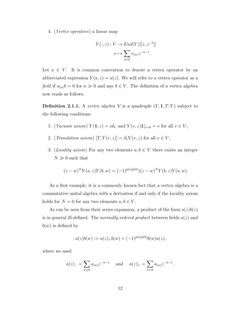
4. (Vertex operators) a linear map

Y (·, z) : V → End(V )[[z, z−1]]

v 7→∑n∈Z

v(n)z−n−1.

Let a ∈ V . It is common convention to denote a vertex operator by an

abbreviated expression Y (a, z) = a(z). We will refer to a vertex operator as a

field if a(n)b = 0 for n 0 and any b ∈ V . The definition of a vertex algebra

now reads as follows.

Definition 2.1.1. A vertex algebra V is a quadruple (V,1, T, Y ) subject to

the following conditions:

1. (Vacuum axiom) Y (1, z) = idV and Y (v, z)1|z=0 = v for all v ∈ V ;

2. (Translation axiom) [T, Y (v, z)] = ∂zY (v, z) for all v ∈ V ;

3. (Locality axiom) For any two elements a, b ∈ V there exists an integer

N 0 such that

(z − w)NY (a, z)Y (b, w) = (−1)p(a)p(b))(z − w)NY (b, z)Y (a, w).

As a first example, it is a commonly known fact that a vertex algebra is a

commutative unital algebra with a derivation if and only if the locality axiom

holds for N = 0 for any two elements a, b ∈ V .

As can be seen from their series expansion, a product of the form a(z)b(z)

is in general ill-defined. The normally ordered product between fields a(z) and

b(w) is defined by

: a(z)b(w) := a(z)+b(w) + (−1)p(a)p(b)b(w)a(z)−

where we used

a(z)− =∑n≥0

a(n)z−n−1 and a(z)+ =

∑n<0

a(n)z−n−1.

12

Acting on an element v ∈ V shows1 that the expression : a(z)b(z) : is well

defined. In case of multiple fields the normally ordered product is defined

recursively

: c0(z)c1(z) · · · cn(z) :=: c0(z) (: c1(z) · · · cn(z) :) :

Let a, b, c0, . . . , cN−1 be elements of the vertex algebra’s underlying vector

space. The following expression is known as the operator product expansion

(OPE)

a(z)b(w) =N−1∑i=0

ci(w)

(z − w)i+1+ : a(z)b(w) : .

It is common practice to abbreviate this expression by writing an equivalence

up to terms which are regular in the limit z → w, i.e. the above expression

will be abbreviated by

a(z)b(w) ∼N−1∑i=0

ci(w)

(z − w)i+1.

A vertex algebra is V strongly generated if there exist fields c0(z), c1(z), . . . , cn(z) ∈

V such that all fields in V can be written as a normally ordered product of the

form

: ∂i0c0(z)∂i1c1(z) · · · ∂incn(z) : .

Many of the vertex algebras encountered in this thesis contain an element

L(z) =∑

n Lnz−n−2 the modes of which statisfy the relations of the Virasoro

algebra

[Lm, Ln] = (m− n)Lm+n +C

12(m3 −m)δm+n,0.

A vertex algebra containing such an element will be refered to as a vertex

operator algebra (VOA). For all vertex operator algebras and their modules

considered here, the element L0 acts semisimply and the VOA itself is given

a grading by the L0-action. In case of a vertex (operator) algebra that is

strongly generated by the fields c0(z), c1(z), . . . , cn(z) we say that the VOA is

of type W(d0, . . . , dn) where di is the grading of the field ci(z). Note that the

grading need not necessarily coincide with the grading under the L0-action.

1This is not obvious from the exposition given here. For details we refer to the standardtextbooks stated in the beginning of this section.

13

Further definitions such as vertex subalgebra, ideal, module, etc. are

straight forward and will be omitted. Further details can be found in the

references stated in the beginning of this section.

Let G be a group and let V be a vertex algebra which is a G-module

where the group action is given by automorphisms. The fixed points under

this action, denoted by VG, form a sub vertex algebra VG ⊂ V . This vertex

algebra is commonly refered to as a G-orbifold.

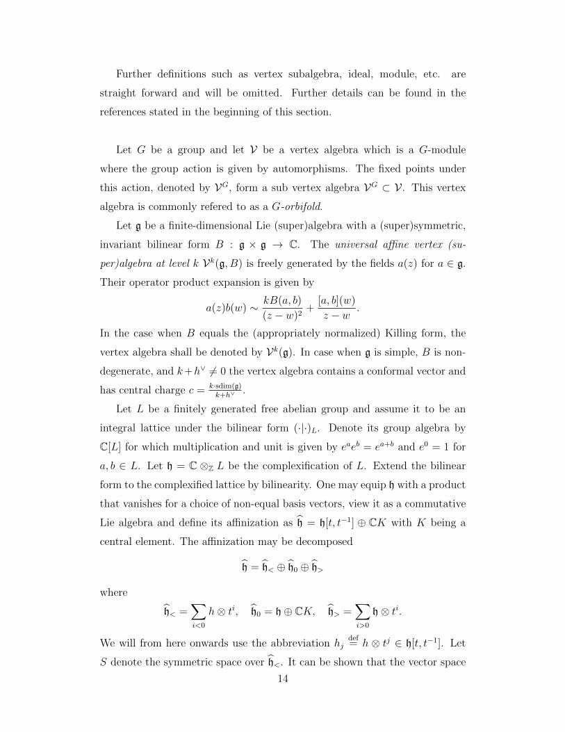
Let g be a finite-dimensional Lie (super)algebra with a (super)symmetric,

invariant bilinear form B : g × g → C. The universal affine vertex (su-

per)algebra at level k Vk(g, B) is freely generated by the fields a(z) for a ∈ g.

Their operator product expansion is given by

a(z)b(w) ∼ kB(a, b)

(z − w)2+

[a, b](w)

z − w.

In the case when B equals the (appropriately normalized) Killing form, the

vertex algebra shall be denoted by Vk(g). In case when g is simple, B is non-

degenerate, and k+h∨ 6= 0 the vertex algebra contains a conformal vector and

has central charge c = k·sdim(g)k+h∨

.

Let L be a finitely generated free abelian group and assume it to be an

integral lattice under the bilinear form (·|·)L. Denote its group algebra by

C[L] for which multiplication and unit is given by eaeb = ea+b and e0 = 1 for

a, b ∈ L. Let h = C ⊗Z L be the complexification of L. Extend the bilinear

form to the complexified lattice by bilinearity. One may equip h with a product

that vanishes for a choice of non-equal basis vectors, view it as a commutative

Lie algebra and define its affinization as h = h[t, t−1] ⊕ CK with K being a

central element. The affinization may be decomposed

h = h< ⊕ h0 ⊕ h>

where

h< =∑i<0

h⊗ ti, h0 = h⊕ CK, h> =∑i>0

h⊗ ti.

We will from here onwards use the abbreviation hjdef= h ⊗ tj ∈ h[t, t−1]. Let

S denote the symmetric space over h<. It can be shown that the vector space

14

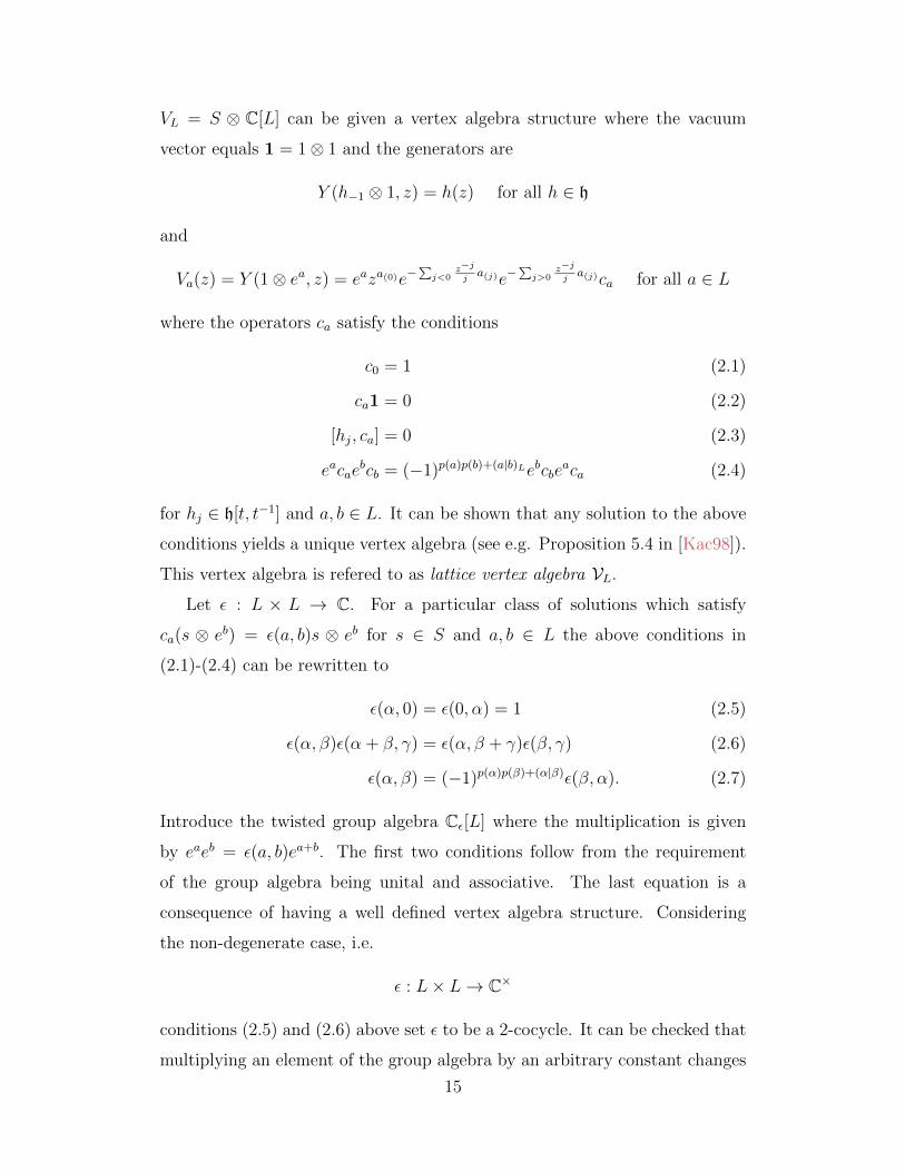
VL = S ⊗ C[L] can be given a vertex algebra structure where the vacuum

vector equals 1 = 1⊗ 1 and the generators are

Y (h−1 ⊗ 1, z) = h(z) for all h ∈ h

and

Va(z) = Y (1⊗ ea, z) = eaza(0)e−∑j<0

z−jja(j)e−

∑j>0

z−jja(j)ca for all a ∈ L

where the operators ca satisfy the conditions

c0 = 1 (2.1)

ca1 = 0 (2.2)

[hj, ca] = 0 (2.3)

eacaebcb = (−1)p(a)p(b)+(a|b)Lebcbe

aca (2.4)

for hj ∈ h[t, t−1] and a, b ∈ L. It can be shown that any solution to the above

conditions yields a unique vertex algebra (see e.g. Proposition 5.4 in [Kac98]).

This vertex algebra is refered to as lattice vertex algebra VL.

Let ε : L × L → C. For a particular class of solutions which satisfy

ca(s ⊗ eb) = ε(a, b)s ⊗ eb for s ∈ S and a, b ∈ L the above conditions in

(2.1)-(2.4) can be rewritten to

ε(α, 0) = ε(0, α) = 1 (2.5)

ε(α, β)ε(α + β, γ) = ε(α, β + γ)ε(β, γ) (2.6)

ε(α, β) = (−1)p(α)p(β)+(α|β)ε(β, α). (2.7)

Introduce the twisted group algebra Cε[L] where the multiplication is given

by eaeb = ε(a, b)ea+b. The first two conditions follow from the requirement

of the group algebra being unital and associative. The last equation is a

consequence of having a well defined vertex algebra structure. Considering

the non-degenerate case, i.e.

ε : L× L→ C×

conditions (2.5) and (2.6) above set ε to be a 2-cocycle. It can be checked that

multiplying an element of the group algebra by an arbitrary constant changes

15

ε by a coboundary. As we are interested in a vertex algebra structure only up

to isomorphism it follows that ε is an element of the second group cohomol-

ogy with coefficients in C×. Hence, isomorphic vertex algebra structures are

determined by an element ε ∈ H2(L,C×) which in addition satisfies the last

condition in (2.7). A vertex algebra structure over the vector space S⊗Cε[L] is

unique up to isomorphism and in particular independent of the choice of ε by

[Kac98, Theorem 5.5a]. Furhermore, one can construct such a vertex algebra

structure choosing ε : L×L→ ±1 by [Kac98, Theorem 5.5b]. It can be seen

from this that the above procedure leads to a central extension of the lattice

L

0→ Z/2Z→ L→ L→ 0.

The lattice vertex algebra in this particular case will be refered to as the lattice

vertex superalgebra VL.

We end this introduction by providing examples of vertex algebras which

will be encountered throughout this work.

Example 2.1.2. The Heisenberg vertex algebra H(n) is freely generated by

even fields hi(z) for i = 1, . . . , n and their non-regular OPEs are given by

hi(z)hj(w) ∼ δi,j(z − w)2

.

Example 2.1.3. The free fermion vertex algebra F(n) is freely generated by

odd fields φi(z) for i = 1, . . . , n and their non-regular OPEs are given by

φi(z)φj(w) ∼ δi,j(z − w)

.

Example 2.1.4. The bc-system E(n) is a vertex algebra that is isomorphic to

F(2n) and freely generated by odd fields bi(z), ci(z) for i = 1, . . . , n and their

non-regular OPEs are given by

bi(z)cj(w) ∼ δi,j(z − w)

and ci(z)bj(w) ∼ δi,j(z − w)

.

Example 2.1.5. The βγ-system S(n) is a vertex algebra that is freely gen-

erated by even fields βi(z), γi(z) for i = 1, . . . , n and their non-regular OPEs

are given by

βi(z)γj(w) ∼ δi,j(z − w)

and γi(z)βj(w) ∼ − δi,j(z − w)

.

16

2.2 The chiral de Rham complex and invariant

theory

It is hard to anticipate from their definition that vertex algebras exhibit con-

nections to geometry. One of them is that any smooth manifold admits a

vertex algebra valued sheaf. Its introduction will be the subject of this sec-

tion. In doing so we will closely follow [MSV99] where the construction has

first appeared and adopt their notation. Note that contrary to examples 2.1.4

and 2.1.5 the set of strong generators of the vertex algebras E(n) and S(n) are

given by φi(z), ψi(z)ni=1 and ai(z), bi(z)ni=1, respectively. Some additional

background will be given only as far as is necessary.

Consider the Heisenberg algebra H and the Clifford algebra C of rank 2N

[aim, bjn] = δi,jδm+n,0 · C and [φim, ψ

jn]+ = δi,jδm+n,0 · C

for i, j = 1, . . . , N . As seen in the previous section each of their associated

vertex algebras - denote them VN and ΛN - allows for a conformal element with

its central charge being equal to 2N and −2N , respectively. Straightforwardly,

the central charge of the vertex algebra over the tensor product ΩN = VN ⊗

ΛN vanishes and the conformal element is simply the sum of the conformal

elements of both sub vertex algebras. It is well known that the vertex algebra

ΩN contains a vertex algebra which is an extension of the Virasoro algebra. In

particular, this vertex algebra is generated by 2 even and 2 odd fields. Apart

from the Virasoro element, the vectors associated to these fields are

J =N∑i=1

φi0ψi−1, Q =

N∑i=1

ai−1φi0, G =

N∑i=1

ψi−1bi−1

17

with their OPEs being defined as follows

T (z)T (w) ∼ 2T (w)

(z − w)2+∂wT (w)

(z − w)

T (z)J(w) ∼ − d

(z − w)3+

J(w)

(z − w)2+∂wJ(w)

(z − w)

T (z)Q(w) ∼ Q(w)

(z − w)2+∂wQ(w)

(z − w)

T (z)G(w) ∼ 2G(w)

(z − w)2+∂wG(w)

(z − w)

J(z)J(w) ∼ d

(z − w)2

J(z)Q(w) ∼ Q(w)

(z − w)

J(z)G(w) ∼ − G(w)

(z − w)

Q(z)G(w) ∼ d

(z − w)3+

J(w)

(z − w)2+

T (w)

(z − w)

(2.8)

There exist two important endomorpisms of ΩN

F = J0 =N∑i=1

∞∑n=−∞

: φinψi−n : and d = −Q0 = −

N∑i=1

∞∑n=−∞

: ainφi−n :

which are commonly refered to as the fermionic charge operator and the chiral

de Rham differential. The relations

[F, φin] = φin, [F, ψin] = −ψin, [F, ain] = 0, [F, bin] = 0

and F1 = 0 can be infered from the vertex algebra structure. This allows for

a vector space decomposition

ΩN =∞⊕

j=−∞

ΩjN for Ωj

N = ω ∈ ΩN |Fω = jω

from which one is quick to see that Ω0N admits a vertex algebra structure.

Observe that the OPE of the field Q(z) with itself is regular which implies that

d2 = 0 and so indeed a differential. Moreover, it holds that this endomorphism

increases the fermionic charge by 1

d : ΩiN → Ωi+1

N .

18

Now, let Ω(AN) =⊕N

j=0 Ωj(AN) denote the algebraic de Rham complex

of the affine space AN . In what follows, note that Λ[φ10, . . . , φ

N0 ] denotes the

exterior algebra on the symbols φ10, . . . , φ

N0 and is a sub-algebra of C. There is

an obvious isomorphism of dg-algebras

ΩN∼= C[b1

0, . . . , bN0 ]⊗ Λ[φ1

0, . . . , φN0 ]

where the left hand side can be identified with the right hand side. Under this

identification note that b10, . . . , b

N0 label the coordinate functions and φ1

0, . . . , φN0

their differentials. Furthermore, the de Rham differential can be written as

ddR =N∑i=1

ai0φi0.

It can be shown (see Theorem 2.4 in [MSV99]) that the embedding of com-

plexes

(Ω(AN), ddR) → (ΩN , d) (2.9)

is compatible with the differentials and a quasi-isomorphism.2 The complex

(ΩN , d) is suggestively refered to as the chiral de Rham complex.

Let B = C[b10, . . . , b

N0 ] and denote its completion under the l-adic topology

by B. It is immediate that B ⊂ H is a subalgebra and H a B-module. One

can associate a vertex algebra structure to the algebra

H = B ⊗B H

as follows: By the obvious one-to-one mapping, any element of the vacuum

module of H can be written as a finite sum of elements of the form f(b0)g(a, b)

where f(b0) ∈ B is a formal power series in the letters b10, . . . , b

N0 and g(a, b) ∈

H is a monomial in the letters a1i1, . . . , aNiN , b

1j1, . . . , bNjN for i1, . . . , iN < 0 and

j1, . . . , jN ≤ 0. In particular, the definition of Y (g(a, b), z) is the same as in

the definition of the vertex algebra structure over H. For the remaining cases

it can be shown that the assignments

Y (f(b0), z) = Y (f(b10, . . . , b

N0 ), z) = f(b1

0(z), . . . , bN0 (z))

2See Theorem 4.4 in [MSV99] for a stronger statement for sheaves in the algebraic,complex analytic, and C∞ setting.

19

and

Y (f(b0)g(a, b), z) =: Y (f(b0), z)Y (g(a, b), z) :

yield a well defined map

Y : H → End(H)[[z, z−1]].

It follows immediately that the vacuum element can be defined as the image

of the vacuum element under the natural embedding H → H. Furthermore,

the existence of a Virasoro element follows by the same argument.

Given the now seemingly close connection to geometry, one may wonder

how a vertex algebra structure can be given when considering localization

Hf = Bf ⊗B H

for a non-zero polynomial f ∈ B. Let Y (f, z) =∑∞

n=−∞ fnz−n. Then

Y (f−1, z) =1

f0 +∑

n6=0 fnz−n =

1

f0

∞∑i=0

(f−1

0

∑n 6=0

fnz−n

)i

is a well defined vertex operator by the above construction provided that f0 is

invertible and it follows that a vertex algebra structure can be associated to

Hf . The above discussion culminates in the following: Let X equal the affine

scheme Spec(B) and consider the quasi-coherent sheaf Och that corresponds to

the B-moduleH. The above construction shows that a vertex algebra structure

can be defined over the open set Uf = Spec(Bf ) in the Zariski topology that is

an associated vertex algebra to Hf = Γ(Uf ,Och). This defines a vertex algebra

valued presheaf since the restriction morphism Hg → Hf for an embedding

Uf → Ug yields a morphism of vertex algebras. One can check that this

construction defines a vertex algebra valued sheaf. In a similar way as above

a vertex algebra structure can be associated to

ΩN = B ⊗B ΩN .

The corresponding vertex algebra valued sheaf is denoted by Ωch. One can de-

fine a partial ordering on the monomials in the tensor product of the Heisenberg

and Clifford algebra which induces a filtration on the vector spaces associated

20

to fields of fixed conformal weight. The associated graded pieces are direct

sums of symmetric powers of the tangent bundle, exterior powers of the bun-

dle of one-forms, and tensor products of said objects.

Remark 2.2.1. Regarding ΩN one can replace B with any commutative B-

algebra that is aDer(B)-module extending which restricts to the natural action

on the subalgebra B. Regarding applications, it follows that one may define a

corresponding sheaf Ωch in the algebraic, complex analytic or smooth setting.

Let X be a smooth scheme of finite type over C. It was shown in [MSV99]

that the global sections of the sheaf Ωch canonically form a conformal vertex

algebra in the complex analytic framework which can be lifted to a vertex

algebra containing the fields J(z), Q(z) and G(z) as given above if the first

Chern class vanishes. It was further shown that the fermionic charge operator

F and the chiral de Rham differential d are well defined endomorphisms of

Ωch which implies that the chiral de Rham complex (Ωch, d) is a complex of

sheaves that are graded by the fermionic charge. In the C∞ setting a simi-

lar picture holds. In case of a Riemannian manifold the sheaf Ωch contains a

N = 1 structure, in case of a Kahler metric and a Ricci-flat manifold it can

be lifted to a N = 2 structure, and if the manifold is hyper-Kahler it further

lifts to a N = 4 structure [BHS08] with central charge c = 3dimC(X).

The question that is being addressed and answered in chapter 4 is funda-

mentally a problem within the framework of invariant theory. Consider the

following: Let G be a linearly reductive group, V a finite dimensional G-

module over a field k, k[V ] the ring of polynomial functions on V and k[V ]G

the subring of G-invariant polynomials. In 1893 Hilbert proved that C[V ]G is

finitely generated. A fundamental problem is then to find generators and re-

lations for the subring k[V ]G. The Basis Theorem, Nullstellensatz and Syzygy

Theorem were introduced by Hilbert in connection to this problem. Now, con-

sider the module W = ⊕j∈SVj where we assume that Vj ∼= V for all j ∈ S0 ⊆ S

and Vj ∼= V ∗ for all j ∈ S\S0. Let R = C[W ]G. For G a classical group and

S of finite cardinality, Weyl’s first fundamental Theorem [Wey46] provides a

21

set of generators for R. Furthermore, his second fundamental Theorem (see

op. cit.) yields generators for the ideal of relations on R. In this thesis we are

mainly (but not exclusively) assuming G to be finite.

Example 2.2.2. Let G = Z/2Z and V the one-dimensional non-trivial rep-

resentation. Take S = N and let xj be a basis for Vj for all j ∈ S. Then

R = C[W ]Z/2Z = C[x1, x2, x3, . . . ]Z/2Z is the subalgebra of R of even degree.

The first fundamental Theorem states that the generators of R can be given

by gi,j = xixj for i ≤ j. The second fundamental Theorem states that the

ideal of relations is generated by gi,jgk,l − gi,kgj,l.

Consider the Heisenberg vertex algebra H = H(1) and denote its strong

generator by h(z). A basis of the underlying vector space of H is given by

the set 1 ∪ : ∂j1h(z) · · · ∂jkh(z) : |0 ≤ j1 ≤ · · · ≤ jk∞k=1 via the state-

field correspondence. Let g denote the generator of the automorphism group

Aut(H) ∼= Z/2Z which acts via g(h(z)) = −h(z). The space of states of

H is linearly isomorphic to the polynomial ring C[x0, x1, . . . ] where xi ↔

∂ih(z). Comparing with example 2.2.2 we see that R ∼= HZ/2Z, hence a set

of strong generators corresponding to gi,j is given by the quadratics ωi,j =:

∂ih(z)∂jh(z) : for i ≤ j. Note that there exist further relations among the

generators of the polynomial ring due to the existence of a differential by the

virtue of the vertex algebra. This manifests itself in the relation ∂xi = xi+1

which induces a relation on the strong generators of R and HZ/2Z. Thus, a

minimal generating set on R as a differential algebra is given by g0,2j|j ≥

0. On the contrary, HZ/2Z is strongly generated by ω0,2j|j ≥ 0, however,

this strong generating set is not minimal. As shown in [DN99] the orbifold

HZ/2Z is of type W(2, 4) and a minimal strong generating set can be given by

ω0,0, ω0,2. Why is this so? Note the following relation

ω0,4 = −4

5(: ω0,0ω1,1 : − : ω0,1ω0,1 :) +

7

5∂2ω0,2 −

7

30∂4ω0,0

= −2

5: ω0,0∂

2ω0,0 : +4

5: ω0,0ω0,2 : +

1

5: ∂ω0,0∂ω0,0 : +

7

5∂2ω0,2 −

7

30∂4ω0,0

and observe its similarity to a generator of the ideal of relations in the G-

invariant subring in example 2.2.2. The ”classical” relation g0,0g1,1−g0,1g0,1 = 0

22

does not vanish in the vertex algebraic framework : ω0,0ω1,1 : − : ω0,1ω0,1 : 6= 0.

In a similar way one can find that the second fundamental Theorem induces

relations ω0,2j+4 = Pj(ω0,0, ω0,2) for j ≥ 0. For further information onH(n)O(n)

we refer to chapter 5 in [Lin13].

In [LL07] Lian and Linshaw introduced the proper framework to deal with

this type of problem by introducing a functor from a certain category of vertex

algebras to the category of supercommutative rings with a differential which

exhibits a reconstruction property such that the problem of finding a minimal

strong generating set can be reduced to finding relations in certain rings. This

will be made precise and used heavily in chapter 4.

2.3 The quantum Drinfeld-Sokolov reduction

and W-algebras

Constructing a vertex algebra can be done in many ways. Some of them are

grounded in Lie theory, an example of which being the affine vertex algebra

Vk(g) which has been introduced at the beginning of this chapter. Another

class of vertex algebras are the so-called W-algebras W(g) which can be seen

as an affinization of the center Z(g) of the universal enveloping algebra U(g).

As the main objects of study in chapter 6 are W-algebras let us briefly recall

their definition. In doing so we follow the exposition given in [KRW03] and

[KW04, KW05]. For another realization of W-algebras see [Gen17] where it

is shown that Wk(g, x, f) at generic level k is isomorphic to the intersection

of kernels of certain operators, acting on the tensor vertex superalgebra of an

affine vertex superalgebra and a neutral free superfermion vertex superalgebra.

Let g be a simple finite-dimensional Lie superalgebra equipped with an in-

variant non-degenerate supersymmetric even bilinear form (·|·). Furthermore,

let x, f ∈ g such that (i) f is even with [x, f ] = −f , (ii) adx is diagonalizable

with eigenvalues in 12Z such that the eigenvalues on the centralizer of f in

g - from here onwards denoted by gf - are non-positive, and (iii) the map

adf : gj → gj−1 is injective for j ≥ 12

and surjective for j ≤ 12. It follows that

23

there exists a vector space decomposition

g = g+ ⊕ g0 ⊕ g− where gj = g ∈ g|[x, g] = jg

with g+ =⊕

j>0 gj and g− =⊕

j<0 gj. It is clear that h ⊂ g0.

Next we introduce 3 vertex algebras associated to this datum; the first

being the universal affine vertex algebra V k(g) associated to the affinization of

the Lie algebra g and the bilinear form (·|·). The bilinear form 〈·|·〉f definied

via

〈a|b〉f = (f |[a, b])

is even and skew-supersymmetric. It follows from (iii) and the non-degeneracy

of (·|·) that this bilinear form is also non-degenerate on g 12. Let Ane

∼= g 12

be

a vector superspace with a bilinear form given by the tuple 〈·|·〉f and denote

its Clifford affinization by Ane. F (Ane) denotes the associated vertex algebra

of neutral free fermions. Lastly, let A ∼= π(g+) and A∗ ∼= π(g∗+) be two vector

superspaces where π is a homomorphism of vector superspaces which restricts

to isomorphisms of vector spaces but exchanges the parity of all elements

(wherever defined) of a superspace. Let Ach = A⊕A∗ be a vector superspace

together with a skew-supersymmetric bilinear form defined by

〈A|A〉 = 〈A∗|A∗〉 = 0 and 〈a|b〉 = b(a) for a ∈ A, b ∈ A∗.

It is clear that this form is non-degenerate. F (Ach) denotes the vertex algebra

of charged free fermions associated to the Clifford affinization Ach.

The object of interest now is the vertex algebra

Ck(g, x, f) = V k(g)⊗ F (Ach)⊗ F (Ane)

for which we assume that the level is non-critical, i.e. k 6= −h∨. This vertex

algebra has an induced grading

C•k(g, x, f) = V k(g)⊗ F •(Ach)⊗ F (Ane)

given by the charge gradation. Note that C0k(g, x, f) ⊂ Ck(g, x, f) is a ver-

tex subalgebra. It can be shown that there exists a field d(z) ∈ Ck(g, x, f)

depending on f for which

[d(z), d(w)] = 0 and [d0, Cmk (g, x, f)] ⊂ Cm−1k (g, x, f)

24

where d0 = Res (d(z)). The former statement implies that d20 = 0, hence

(C•k(g, x, f), d0) is a chain complex for which the cohomological grading is

given by the charge. The cohomology, denoted here by H•k(g, x, f), is a vertex

superalgebra with an apropriate Z-grading (which differs to the grading by

charge). Moreover, the cohomology is acyclic. i.e. H ik(g, x, f) = 0 for i 6= 0

[KW04, Theorem 4.1 (c)]. The resulting vertex algebra H0k(g, x, f) is denoted

by Wk(g, x, f) and refered to as the quantum Drinfeld-Sokolov reduction of

the quadruple (g, x, f, k). In addition, it contains a Virasoro field. Let uii∈Sbe a basis of g+ that is compatible with its grading, i.e. [x, ui] = iui. The

central charge c is given by (see Theorem 2.2 (a) in [KRW03])

c(g, x, f, k) =k sdim(g)

k + h∨− 12(x|x)−

∑i∈S

(−1)p(ui)(12i2− 12i+ 2) +1

2sdim(g 1

2).

(2.10)

For a basis gi of gf that is compatible with the grading gf =⊕

j gfj induced

from the decomposition of g as given above, the vertex algebra Wk(g, x, f)

is strongly generated by fields Jgi(z) of conformal weight 1 + i for gi ∈ gf−i

[KW04, Theorem 4.1 (b)].

Remark 2.3.1. Note that it follows from condition (i) that f is a nilpotent

element. Hence, by the Jacobson-Morozov theorem, it may be embedded in

a sl2-triple e, f, h and all such triples are conjugate under an action of the

centralizer gf . Taking the elements x, f to be elements of an sl2-triple has

implications on the grading. We will not go into detail here and simply refer

to [KRW03] where gradings with and without this property are discussed from

section 2.4 onwards.

Remark 2.3.2. Recall that we have assumed non-criticality of the level k.

W-algebras at the critical level have been explored in the literature. See

for example [Ara12] where it is shown that the center of Wk(g, f) for the

critical level k coincides with the Feigin-Frenkel center of the affine Lie algebra

associated with g.

This construction can be extended as follows: Let M be a restricted g-

module. Any such module extends to a V k(g)-module which trivially extends

25

to a Ck(g, x, f)-module M ⊗ F (Ach) ⊗ F (Ane). Following the previous steps,

the module

C•(M) = M ⊗ F •(Ach)⊗ F (Ane)

has a Z-grading given by charge, (C•(M), d0) is a chain complex of Ck(g, x, f)-

modules and thus its cohomology is a direct sum ofWk(g, x, f)-modulesH(M) =⊕j∈ZH

j(M). In particular, this construction yields a functor

Hf : Rep(g)res → Rep(Wk(g, x, f))

from the category of restricted g-modules to the category of Wk(g, x, f)-

modules. This functor maps any integrable g-module to zero (cf. [Ara05,

KRW03]). Moreover, it has been shown that this functor is exact and maps

any irreducible module to zero or to an irreducible module [Ara04, Ara07].3

3See [Ara05] for an earlier result where it is proved that the functor Hf preserves irre-ducibility in the case of Wk(g, fθ)-modules where fθ is the root vector corresponding to thelowest root −θ of g.

26

Chapter 3

Self-dual vertex operatorsuperalgebrasand superconformal field theory

3.1 Introduction

The elliptic genus of a complex K3 surface X is a weak Jacobi form of weight

zero and index one. It may be realized in the following three ways: via the chi-

ral de Rham complex of X [BHS08, Hel09, Bor01, BL00], as the S1-equivariant

χy-genus of the loop space of X [Hir78, Hoh91, Kri90], and as a trace on the

Ramond-Ramond sector of a sigma model on X [EOTY89, DY93, Wit94].

The small N = 4 superconformal algebra at central charge c = 6 appears in

each of these three pictures. Firstly, it is the algebra of global sections of the

chiral de Rham complex [Son16, Son15]. Secondly, the χy-genus can be viewed

as a virtual module for a certain vertex operator superalgebra that contains

this Lie superalgebra [CH14, TZZ99]. Finally, it appears as a supersymmetry

algebra of the string theory sigma model [ET88b]. (We refer to [Wen15] for a

recent detailed review of these topics.)

The K3 elliptic genus and the N = 4 superconformal algebra were ab-

sorbed into the orbit of moonshine when Eguchi–Ooguri–Tachikawa [EOT11]

suggested a relationship between the largest Mathieu group, M24, and char-

acter contributions of the N = 4 superconformal algebra to the K3 elliptic

genus. This ignited a resurgence of interest in connections between string the-

MSC2010: 17B69, 17B81, 20C34.

27

ory, modular forms and finite groups. Umbral moonshine [CDH14a, CDH14b,

DGO15b], Thompson moonshine [HR16, GM16] and the recently announced

O’Nan moonshine [DMO17] all belong to the quickly developing legacy of this

Mathieu moonshine observation, although the connections to string theory are

so far more obscure in the latter two cases. We refer to [DGO15a] for a fuller

review, more references, and for comparison to the original monstrous moon-

shine [CN79, Tho79a, Tho79b] that appeared in the 1970s.

By now there are indications that Mathieu and monstrous moonshine are

interrelated. An instance of this, and a primary motivation for the present

work is [DM16], wherein the K3 elliptic genus apparently makes a fourth

appearance: as a trace function on the moonshine module [Dun07, DM15]

for Conway’s group, Co0 [Con68, Con69]. On the one hand, this Conway

moonshine module—a vertex operator superalgebra with N = 1 structure—

is a direct supersymmetric analogue of the monstrous moonshine module of

Frenkel–Lepowsky–Meurman [FLM84, FLM85, FLM89]. It manifests a genus

zero property for Co0 [DM15], just as the monstrous moonshine module does

for the monster [Bor92]. On the other hand, M24 is a subgroup of Co0, and

the Conway moonshine construction of the K3 elliptic genus may be twined

by (most) elements of M24. In many, but not all instances the resulting trace

functions coincide with those that arise in Mathieu moonshine.

This tells us that the Conway moonshine module comes close to providing

a vertex algebraic realization of the as yet elusive Mathieu moonshine module,

whose structure as a representation of M24 was conjecturally determined in

[Che10, GHV10b, GHV10a, EH11], and confirmed in [Gan16]. The Conway

moonshine module has been used to realize analogues of the Mathieu moon-

shine module for other sporadic simple groups in [CDD+15, CHKW15]. See

[TW15b, TW13, TW15a, GKH17, TW17] for the development of a promising

geometric approach to the problem.

The Conway moonshine module is also connected to string theory on K3

surfaces. As is explained in [DM16], the Conway moonshine construction of the

K3 elliptic genus may also be twined, in an explicitly computable way, by any

automorphism of a K3 sigma model that preserves its supersymmetry. Such

28

automorphisms are classified in [GHV12]. It appears that the construction

of [DM16] is (except for a small number of possible exceptions) in agreement

[CHVZ18] with the twined K3 elliptic genera that one expects [CHVZ18] to

arise from string theory. One reason this is surprising is that K3 sigma models,

and in particular their automorphisms, are difficult to construct in general (cf.

e.g. [NW01]). The Conway moonshine module seems to serve as a shortcut, to

certain computations which might otherwise require the explicit construction

of sigma models.

In view of these connections it is natural to ask how the Conway moon-

shine realization of the K3 elliptic genus is related to the three we began with

above. Katz–Klemm–Vafa [KKV99] conjectured a method for computing the

Gromov–Witten invariants of a K3 surface in terms of the χy-genera of its sym-

metric powers, and the generating function of these χy-genera can be realized

in terms of a lift of the K3 elliptic genus. So the second mentioned realiza-

tion of the K3 elliptic genus, as a generalization of Hirzebruch’s χy-genus,

suggests a connection between Conway moonshine and enumerative geometry.

This perspective is developed in [CDHK17], where equivariant counterparts to

the conjecture of Katz–Klemm–Vafa are formulated, which explicitly describe

equivariant versions of Gromov–Witten invariants of K3 surfaces. The con-

jecture of Katz–Klemm–Vafa was proved recently by Pandharipande–Thomas

[PT16]. Katz–Klemm–Pandharipande [KKPT16] have extended the the con-

jecture of Katz–Klemm–Vafa to refined Gopakumar–Vafa invariants. Con-

jectural descriptions of equivariant refined Gopakumar–Vafa invariants of K3

surfaces are also formulated in [CDHK17].

In this work we develop the relationship between Conway moonshine and

the third mentioned realization, in terms of K3 sigma models. We do this

by formalizing a new relationship between vertex algebra and conformal field

theory, and by realizing the Conway moonshine module, and other vertex

operator superalgebras, in examples.

Traditionally, vertex operator algebras satisfying suitable conditions are

considered to define “chiral halves” of conformal field theories. More specif-

ically, the bulk Hilbert space of a conformal field theory may be regarded as

29

(a completion of) a suitable sum of modules for a tensor product of vertex

operator algebras (cf. [Hua92, Gab00, Wen15]). The alternative viewpoint

we pursue here develops from the observation that a bulk Hilbert space of a

conformal field theory, taken as a whole, resembles a self-dual vertex operator

algebra. We explain this observation more fully in §3.4.1. It motivates our

Main Question: Can a self-dual vertex operator algebra be iden-

tified with a bulk conformal field theory in some sense?

We answer this question positively by formulating the notion of potential (bulk)

conformal field theory (cf. Definition 3.4.1) and by identifying self-dual vertex

operator algebras as examples (cf. Propositions 3.5.1 and 3.5.3). In fact, we

formulate supersymmetric counterparts to potential conformal field theories

as well (cf. Definitions 3.4.3 and 3.4.6), and find more examples amongst self-

dual vertex operator superalgebras (cf. Theorems 3.5.6, 3.5.8 and 3.5.9). To

support the analysis we also present a classification result (Theorem 3.3.1) for

self-dual vertex operator superalgebras with central charge up to 12.

Equipped with the notion of potential bulk superconformal field theory we

relate the Conway moonshine module to four superconformal field theories in

§3.5. One of these is the superconformal field theory underlying the tetrahedral

K3 sigma model (cf. §3.5.3), which was analyzed in detail by Gaberdiel–

Taormina–Volpato–Wendland [GTVW14] (see also [TW17]). Another is the

Gepner model (1)6 (cf. §3.5.4), and it is clear that there are further interesting

examples waiting to be considered, that may shed more light on the role of

Conway moonshine in K3 string theory.

An implication of our analysis is that there should be self-dual vertex oper-

ator superalgebras besides the Conway moonshine module that have analogous

relationships to other string theory compacitifcations. In §3.5.2 we identify a

self-dual vertex operator superalgebra—the N = 1 vertex operator superal-

gebra naturally attached to the E8 lattice—which realizes the bulk supercon-

formal field theory underlying a sigma model with a 4-torus as target (cf.

Theorem 3.5.6). Volpato [Vol14] has shown that the supersymmetry preserv-

ing automorphism groups of 4-torus sigma models are subgroups of the Weyl

30

group of the E8 lattice. In light of these results it seems likely that the E8 ver-

tex operator superalgebra that appears in §3.5.3 can serve as a counterpart to

the Conway moonshine module for nonlinear sigma models on 4-dimensional

tori.

It is interesting to compare the approach presented here to recent work

[TW17] of Taormina–Wendland. In loc. cit. the relationship between super-

conformal field theory and vertex operator superalgebra is also reconsidered,

but the starting point is a fully fledged superconformal field theory. A no-

tion of reflection is introduced which, in special circumstances, produces a

vertex operator superalgebra. The superconformal field theory underlying the

tetrahedral K3 sigma model is considered in detail, and it is shown that the

Conway moonshine module arises when reflection is applied in this case. In

this way Taormina–Wendland independently obtain results equivalent to those

we present in §3.5.3. Our notion of potential superconformal field theory serves

to answer the question of what reflection produces from a superconformal field

theory in general, except that a reflected superconformal field theory comes

equipped with extra structure, on account of the richness of the supercon-

formal field theory axioms. For example, the reflected tetrahedral K3 theory

recovers the vertex operator superalgebra structure on the Conway moonshine

module, but also furnishes an intertwining operator algebra structure on the

direct sum of itself with its unique irreducible canonically twisted module (cf.

§4 of [TW17]). Moving forward, we can expect that Taormina–Wendland re-

flection will play a key role in further elucidating the relationships between

superconformal field theories, potential superconformal field theories and ver-

tex operator superalgebras.

We now describe the structure of the article. We present background ma-

terial in §3.2. We explain our conventions on vertex operator superalgebras

in §3.2.1, and we review some modularity results for vertex operator super-

algebras in §3.2.2. We recall the small N = 4 superconformal algebra in

§3.2.3, and describe an explicit construction at c = 6 in §3.2.4. In §3.3 we

establish our classification result for self-dual vertex operator superalgebras

with central charge at most 12. Then in §3.4 we discuss the new relationship

31

between vertex algebra and conformal field theory that motivates this work,

and explain our approach to answering the Main Question. We begin with

conformal field theory in §3.4.1, discuss superconformal field theory in §3.4.2,

and consider superconformal field theories with superconformal structure in

§3.4.3. We present examples of bulk superconformal field theory interpreta-

tions of self-dual vertex operator superalgebras in §3.5. We begin with the

diagonal conformal field theories associated to type D lattice vertex operator

algebras in §3.5.1, and then discuss super analogues of these in §3.5.2. We

discuss the superconformal field theory underlying the tetrahedral K3 sigma

model in §3.5.3, and discuss the relationship between the Conway moonshine

module and the Gepner model (1)6 in §3.5.4.

3.2 Background

3.2.1 Vertex Superalgebra

We assume some familiarity with the basics of vertex (operator) superalgebra

theory. Good references for this include [FB04, FLM89, Kac98, LL04].

We adopt the convention, common in physical settings, of writing (−1)F

for the canonical involution on a superspace W = W even ⊕ W odd, so that

(−1)F |W even = I and (−1)F |W odd = −I. We write Y (a, z) =∑a(k)z

−k−1 for

the vertex operator attached to an element a in a vertex superalgebra W . A

vertex superalgebra W is called C2-cofinite if W/C2(W ) is finite-dimensional,

where C2(W ) := a(−2)b | a, b ∈ W. Following [DLMM98] we say that a ver-

tex operator superalgebra W is of CFT type if the L0-grading W =⊕

n∈ 12ZWn

is bounded below by 0, and if W0 is spanned by the vacuum vector. We as-

sume that W even =⊕

n∈ZWn and W odd =⊕

n∈Z+ 12Wn. A vertex operator

superalgebra that is C2-cofinite and of CFT type is nice (schon) in the sense

of [Hoh07].

Say that a vertex operator algebra is rational if all of its admissible modules

are completely reducible. We refer to [DLM98] for the definition of admissible

module. It is proven in loc. cit. that a rational vertex operator algebra

has finitely many irreducible admissible modules up to equivalence. We say

32

that a vertex operator superalgebra is rational if its even sub vertex operator

algebra is rational. We will apply results from [DZ05] in what follows, so we

should note that our notion of rationality for a vertex operator superalgebra

is stronger than that which appears there. A vertex operator superalgebra

that is rational in our sense is both rational and (−1)F -rational in the sense of

loc. cit. The equivalence of the two notions of rationality is proven in [HA15]

under an assumption on fusion products of canonically twisted modules.

We say that a vertex operator superalgebra W is self-dual if W is rational

(in our sense), irreducible as a W -module, and if W is the only irreducible

admissible W -module up to isomorphism. Note that the term self-dual is

sometimes used differently elsewhere in the literature, to refer to the situation

in which W is isomorphic to its contragredient as a W -module.

According to Theorem 8.7 of [DZ05] a self-dual C2-cofinite vertex operator

superalgebra W has a unique (up to isomorphism) irreducible (−1)F -stable

canonically twisted module. We denote it Wtw. The (−1)F -stable condition

on a canonically twisted module M for W is equivalent to the requirement

of a superspace structure M = M even ⊕ Modd that is compatible with the

superspace structure on W , so that elements of W even and W odd induce even

and odd transformations of M , respectively. Modules that are not (−1)F -

stable will not arise in this work so we henceforth assume the existence of a

compatible superspace structure to be a part of the definition of untwisted

or canonically twisted module for a vertex operator superalgebra. However,

we will not require morphisms of modules to preserve a particular superspace

structure. So for example, if W is a vertex operator superalgebra and Π is the

parity change functor on superspaces then W and ΠW are not isomorphic as

superspaces, but we do regard them as isomorphic W -modules.

Write VL for the vertex superalgebra attached to an integral lattice L,

which is naturally a vertex operator superalgebra if L is positive definite. Write

F (n) for the vertex operator superalgebra of n free fermions. According to the

boson-fermion correspondence [Fre81, DM94] the vertex operator superalgebra

attached to Zn is isomorphic to F (2n). So the even sub vertex operator algebra

F (2n)even < F (2n) is isomorphic to the lattice vertex operator algebra attached

33

to the type D lattice

Dn := (x1, . . . , xn) ∈ Zn | x1 + · · ·+ xn = 0 mod 2 . (3.2.1)

The discriminant group of Dn is D∗n/Dn ' Z/2Z × Z/2Z, and we label coset

representatives as follows.

[0] := (0, . . . , 0, 0), [1] :=1

2(1, . . . , 1, 1),

[2] := (0, . . . , 0, 1), [3] :=1

2(1, . . . , 1,−1).

(3.2.2)

Set D+n := Dn ∪ Dn + [1]. Then D+

n is a self-dual integral lattice—the rank

n spin lattice—whenever n = 0 mod 4. It is even if n = 0 mod 8. We have

D+4∼= Z4 and D+

8∼= E8, and D+

12 is the unique self-dual integral lattice of rank

12 such that λ ·λ ≤ 1 implies λ = 0. The lattice vertex operator superalgebras

attached to Dn and D+4n will play a prominent role later on.

Set A1 =√

2Z. We will make use of the fact that D2n admits A2n1 as a sub

lattice. Explicitly, denoting e1 := (1, 0, . . . 0), e2 := (0, 1, . . . , 0), et cetera, we

may take the first copy of A1 to be generated by e1 + en+1, the second copy

to be generated by e1 − en+1, the third copy to be generated by e2 + en+2, et

cetera. In the case that n = 1 this embedding is actually an isomorphism,

D2∼= A1 ⊕ A1. More generally, D2n/A

2n1 embeds in the discriminant group of

A2n1 , which is naturally isomorphic to (Z/2Z)2n ∼= F2n

2 . As such, it is natural

to use binary codewords of length 2n to label cosets of A2n1 in its dual. Given

such a codeword C ∈ F2n2 , define wt(C)—the weight of C—to be the number

of non-zero entries of C. Define a binary code D2n < F2n2 by setting

D2n := C = (c1, . . . , c2n) | ci = cn+i for 1 ≤ i ≤ n,wt(C) = 0 mod 4 .(3.2.3)

We will abuse notation somewhat by also using [i] to denote the following

length 2n codewords,

[0] := (02n), [1] := (1n0n), [2] := (0n−110n−11), [3] := (1n−10n1). (3.2.4)

The next result may be checked directly, and smooths out any conflict

between (3.2.2) and (3.2.4).

34

Lemma 3.2.1. With the above conventions, the image of (D2n + [i])/A2n1 in

F2n2 is D2n + [i] for i ∈ 0, 1, 2, 3.

The above discussion shows, in particular, that A121∼=√

2Z12 embeds in

D+12. In §3.5.4 we will make use of the fact that

√3Z12 also embeds in D+

12.

To see this recall that the (extended) ternary Golay code is a linear sub space

G < F123 of dimension 6 such that if

C ·D :=∑i

cidi (3.2.5)

for C = (c1, . . . , c12) and D = (d1, . . . , d12) then C · D = 0 when C,D ∈ G,

and no non-zero codeword C ∈ G has less than six non-zero entries. These

properties determine G uniquely, up to permutations of coordinates, and mul-

tiplications of coordinates by ±1 (cf. e.g. [CS88]).

We will denote the elements of F3 by 0,+,− when convenient. To obtain

an embedding of√

3Z12 in D+12 fix a copy G of the ternary Golay code in

F123 . Multiplying some components by −1 if necessary we may assume that

(+12) ∈ G. Then there are exactly 11 code words Ci = (ci1, . . . , ci12) ∈ G such

that the first entry of Ci is +1, five further entries are +1, and the remaining

six entries are−1. Set C12 = (+12) and define λi := (λi1, . . . , λi12) for 1 ≤ i ≤ 12

by setting λij = ±12

when cij = ±1. Then the λi all belong to D+12, and satisfy

λi · λj = 3δij. So the λi constructed in this way generate a sub lattice of D+12

isomorphic to√

3Z12.

The discriminant group of√

3Z12 is F123 , so it is natural to consider the

image of D+12/√

3Z12 in F123 . Denote it G+

12. Since D+12 is a self-dual lattice, G+

12

is a linear subspace such that C · D = 0 for C,D ∈ G+12. From the fact that

λ ∈ D+12 can only satisfy λ · λ ≤ 1 if λ = 0 we obtain that G+

12 has no non-zero

words with fewer than six non-zero entries. Applying the uniqueness of the

ternary Golay code we obtain the following result.

Lemma 3.2.2. The image of D+12/√

3Z12 in F123 is a copy of the ternary Golay

code.

35

3.2.2 Modularity

We now review some results on modularity for vertex operator superalgebras.

Zhu proved [Zhu96] that certain trace functions on irreducible modules for

suitable vertex operator algebras span representations of the modular group

SL2(Z). More general modularity results that incorporate twisted modules

have been obtained by Dong–Li–Mason [DLM00], Dong–Zhao [DZ05, DZ10],

and Van Ekeren [Van13]. We will use the extension of [Zhu96, DLM00] to

vertex operator superalgebras established in [DZ05].

To describe the relevant results let W =⊕

n∈ 12ZWn be a rational C2-

cofinite vertex operator superalgebra of CFT type. Let I0 be an index set for

the isomorphism classes of irreducible W -modules, let I1 be an index set for the

isomorphism classes of irreducible canonically twistedW -modules, and set I :=

I0 ∪ I1. Write Mi for a representative (untwisted or canonically twisted) W -

module corresponding to i ∈ I, and choose a compatible superspace structure

Mi = M eveni ⊕ Modd

i for each i ∈ I. For M an untwisted or canonically

twisted W -module define vertex operators on the torus Y [a, z] : M → M((z))

for a ∈ W by requiring that Y [a, z] = Y (a, ez − 1)enz when a ∈ Wn, and

define a[n] ∈ End(M) by requiring Y [a, z] =∑

k a[n]z−n−1. Also, write W =⊕

n∈ 12ZW[n] for the eigenspace decomposition of W with respect to the action

of ω[1], where ω := ω− c24

v, and ω and v are the Virasoro and vacuum elements

of W , respectively.

Theorem 3.2.3 ([DZ05]). Suppose that W is a rational C2-cofinite vertex

operator superalgebra with central charge c. Then with I and Mii∈I as above

there are maps ρij : SL2(Z) → C for i, j ∈ I such that if v ∈ W[n] for some

n ∈ 12Z then

trMi

(o(v)(−1)`F qL0− c

24

)∣∣n

( a bc d ) =∑j∈Ik

ρij ( a bc d ) trMj

(o(v)(−1)

˜F qL0− c24

)(3.2.6)

for ` ∈ Z/2Z and ( a bc d ) ∈ SL2(Z), where k = 1 +a(k+ 1) + c(`+ 1) mod 2 and

˜= 1 + b(k + 1) + d(`+ 1) mod 2 when i ∈ Ik.

36

In (3.2.6) we utilize the usual slash notation from modular forms, setting

(f |n ( a bc d )) (τ) := f(aτ+bcτ+d

)1

(cτ+d)n(3.2.7)

for a holomorphic function f : H→ C and ( a bc d ) ∈ SL2(Z). If W is a rational

C2-cofinite vertex operator algebra then we can apply Theorem 3.2.3 to W

by regarding it as a vertex operator superalgebra with trivial odd part. Then

I0 = I1 and we recover a specialization of Zhu’s results [Zhu96] for W by taking

k = ` = 1 in (3.2.6).

Resume the assumption that W is a rational C2-cofinite vertex operator

superalgebra of CFT type. Define the characters of an untwisted or canonically

twisted W -module M by setting

ch±[M ](τ) := trM((±1)F qL0− c

24

). (3.2.8)

Then taking v to be the vacuum in Theorem 3.2.3 we obtain

chε[Mi]

(aτ + b

cτ + d

)=∑j∈Ik

ρij(γ) chε[Mj](τ), (3.2.9)

for ( a bc d ) ∈ SL2(Z), where ε = (−1)` and ε = (−1)˜.

In this work we will be especially interested in the situation in which a

superspace M is a module for a tensor product V ′ ⊗ V ′′ of vertex operator

superalgebras, and is thus equipped with two commuting actions of the Vira-

soro algebra. We write L′n and L′′n for the Virasoro operators corresponding

to V ′ and V ′′, respectively, and write c′ and c′′ for the corresponding central

charges. Then it is natural to consider the refined characters

ch±

[M ](τ ′, τ ′′) := trM

((±1)F q′

L′0−c′24 q′′

L′′0−c′′24

)(3.2.10)

where q′ := e2πiτ ′ and q′′ := e2πiτ ′′ . Krauel–Miyamoto [KM15] have shown how

Zhu’s theory [Zhu96] extends so as to yield a modularity result for such refined

characters in the vertex operator algebra case. By replacing Zhu’s results with

the appropriate vertex operator superalgebra counterparts from [DZ05] in the

proof of Theorem 1 in [KM15] we readily obtain a direct analogue for vertex

operator superalgebras. Here we require the following special case of this.

37

Theorem 3.2.4 ([DZ05, KM15]). Let W be a rational C2-cofinite vertex op-

erator algebra and suppose that ω = ω′+ω′′ where ω is the conformal vector of

W , and ω′ and ω′′ generate commuting representations of the Virasoro algebra.

Then with I, Mii∈I and ρij(γ) as in (3.2.6) we have

chε[Mi]

(aτ ′ + b

cτ ′ + d,aτ ′′ + b

cτ ′′ + d

)=∑j∈Ik

ρij(γ)chε[Mj](τ

′, τ ′′) (3.2.11)

for ( a bc d ) ∈ SL2(Z). Here k and ˜ are as in (3.2.6), for ε = (−1)` and ε =

(−1)˜.

3.2.3 Superconformal Algebras

In this section we recall some properties of the small N = 4 superconformal

algebra from [Ali99, ET87, ET88a, ET88b]. It is strongly generated by a

Virasoro field T of dimension 2, four odd fields Ga (a = 0, 1, 2, 3) of dimension

32, and three even fields J i (i = 1, 2, 3) of dimension 1. Define

αia,b :=1

2(δa,iδb,0 − δb,iδa,0) +

1

2εiab (3.2.12)

where εijk is totally antisymmetric for i, j, k ∈ 1, 2, 3, normalized so that

ε123 = 1, and defined to be zero if one of the indices is zero. Also let k

be a positive integer and set c = 6k. The operator product algebra in a

representation with central charge c is then

T (z)T (w) ∼12c

(z − w)4+

2T (w)

(z − w)2+∂wT (w)

(z − w), (3.2.13)

T (z)Ga(w) ∼32Ga(w)

(z − w)2+∂wG

a(w)

(z − w), (3.2.14)

T (z)J i(w) ∼ J i(w)

(z − w)2+∂wJ

i(w)

(z − w), (3.2.15)

Ga(z)Gb(w) ∼23cδa,b

(z − w)3−

3∑i=1

8αia,bJi(w)

(z − w)2+

2δa,bT (w)−3∑i=1

4αia,b∂wJi(w)

(z − w),

(3.2.16)

J i(z)Ga(w) ∼

3∑b=0

4αia,bGb(w)

(z − w), (3.2.17)

38

J i(z)J j(w) ∼−1

2kδi,j

(z − w)2+

3∑k=1

εijkJk(w)

(z − w). (3.2.18)

Equivalently, we have the following commutation relations of modes, where

m,n ∈ Z and r, s ∈ Z + 12.

[Lm, Ln] = (m− n)Lm+n =c

12

(M3 −m

)δm+n,0,

[Lm, Gar ] =

(m2− r)Gam+r,

[Lm, Jin] = −nJ im+n,

Gar , G

bs = 2δa,bLr+s −

3∑i=1

4(r − s)αia,bJ ir+s +c

3

(r2 − 1

4

)δa,bδr+s,0,

[J im, Gar ] =

3∑b=0

αia,bGbm+r,

[J im, Jjn] =

3∑k=1

εijkJkm+n −m

k

2δi,jδm+n,0.

(3.2.19)

Note that the currents J i(z) represent the affine Lie algebra of sl2 at level

k, and k is a positive integer in any unitary representation. Often one uses

another basis for these; namely

J(z) := −2iJ1(z), J+(z) := J2(z)− iJ3(z), J−(z) := −J2(z)− iJ3(z).(3.2.20)

Also for the odd currents there is another useful basis:

G−,1(z) := G0(z)− iG1(z), G+,1(z) := −G2(z) + iG3(z), (3.2.21)

G−,2(z) := G2(z) + iG3(z), G+,2(z) := −G0(z) + iG1(z), (3.2.22)

which yields

[J±m, G∓,xr ] = G±,xm+r, [Jm, G

±,xr ] = ±G±,xm+r (3.2.23)

for x ∈ 1, 2.

The mode algebra of the affine Lie algebra of sl2 at level k has a family of

automorphisms, called spectral flow. They are induced from affine Weyl trans-

lations so they are parameterized by the translation lattice which is isomorphic

39

to Z. For ` ∈ Z the corresponding action is denoted σ`, and satisfies

σ`(J±n)

= J±n∓`,

σ` (Jn) = Jn − δn,0`k,

σ` (Ln) = Ln + δn,0

(`

2J0 +

`2k

4

).

(3.2.24)

We may consider twisted modules as in (2.10) of [CR13]. That is, given a

module M for the affine Lie algebra of sl2 at level k let σ∗` be the unique

invertible linear transformation of M such that the action of the mode algebra

satisfies

Xσ∗` (v) = σ∗`(σ−`(X)v

). (3.2.25)

This σ`-twisting of M is isomorphic to M as a module for the mode algebra,

but since the grading is changed they are in general not isomorphic as modules

for the vertex operator algebra Lk(sl2) attached to sl2 at level k. Identification

of the twisted modules can often be achieved via characters.

So we define a character of M by setting

ch[M ](y, u, τ) := trM(ykzJ0qL0− c

24

)(3.2.26)

where z = e2πiu and q = e2πiτ . Then from the action of σ` we see that

ch[σ∗` (M)](y, z, q) = ch[M ](yz`q14`2 , zq

12`, q). (3.2.27)

If k is a positive integer and M is an irreducible integrable highest-weight

module of level k, then the character of M is a component of a vector-valued

Jacobi form and the twisted module can be seen to be isomorphic to the

original one if ` is even. If ` is odd it maps the irreducible integrable highest-

weight module with highest weight j (corresponding to the j + 1 dimensional

representation of sl2) to the one with highest weight k−j. Thus it corresponds

to fusion with the order two simple current module.

We now consider a vertex operator superalgebra V of central charge c = 6k

that contains a commuting pair of sub vertex operator algebras Lk(sl2) and

U , where the Virasoro elements of V and Lk(sl2)⊗ U coincide. We require U

40

to be rational, and suppose that V is of the form

V =⊕i

Lk(λi)⊗ Ui (3.2.28)

where Lk(λi) is the irreducible Lk(sl2)-module with highest weight λi, and Ui is

an irreducible U -module. Further we require that V contain strong generators

for the small N = 4 superconformal algebra at c = 6k. In this situation the

parity of elements in V is given by (−1)J0 where J0 is as in (3.2.20), (3.2.23).

The spectral flow automorphism σ := σ1 extends naturally to V in such a way

that

σ∗(V ) =⊕i

(Lk(λi) Lk(sl2) Lk(λ∗)

)⊗ Ui (3.2.29)

as a Lk(sl2) ⊗ U -module, where Lk(λ∗) denotes the order two simple current

of Lk(sl2), and V is the fusion product for modules over V .

Under spectral flow we have σ−1(L0) = L0 + 12J0 + c

24, so the conformal

weight of the modes G±,xr becomes r ± 12

as endomorphisms on twisted mod-

ules. Especially, the G±,x∓ 12

act with conformal dimension zero, and thus induce

grading-preserving maps from the even part to the odd part of the twisted

module. We compute(G+,1

− 12

+G−,212

)2

=1

2

G+,1

− 12

+G−,212

, G+,1

− 12

+G−,212

= −2L0 + J0

= 2σ−1(L0 −

c

24

).

(3.2.30)

This shows that G+,1

− 12

+ G−,212

is an invertible map from the even conformal

grade n subspace of σ∗(M) to the odd one as long as n− c24

does not vanish.

We summarize this as follows.

Lemma 3.2.5. If M is a V -module and σ∗(M) =⊕

n σ∗(M)n is the grading

of the corresponding twisted module then sdimσ∗(M)n = 0 unless n− c24

= 0.

3.2.4 Free Fields

We now describe a free field realization of the small N = 4 superconformal

algebra at c = 6. Consider the tensor product of the vertex operator super-

algebra of four free fermions with the rank four Heisenberg vertex operator

41

algebra. An action of the compact Lie group SU(2) is given by organizing

both the fermions and bosons in the standard and conjugate representations

of SU(2). By Lemma 3.4 of [CH14] the sub vertex operator superalgebra of

fixed points for this SU(2) action contains the small N = 4 superconformal al-

gebra at c = 6. So by using bosonization we obtain a free field realization of the

small N = 4 superconformal algebra at c = 6 in terms of twelve free fermions.

The precise expression for the latter can be found in §2 of [GTVW14]. In

terms of lattice vertex operator superalgebras this free field realization may

be described as follows.

The vertex operator superalgebra of four free fermions may be identified

with the lattice vertex operator superalgebra associated to Z2. We have Z2 =

D2 ∪ (D2 + [2]) in the notation of §3.2.1, and the exceptional isomorphism

D2∼= A1 ⊕ A1. So VD2

∼= VA1 ⊗ VA1 . Four free fermions are thus the simple

current extension of VA1 ⊗ VA1 by the unique simple current with dimension

12. The free field realization in terms of twelve free fermions can be inspected

to be a sub vertex operator superalgebra of

V ⊗3D2⊕ V ⊗3

D2+[2], (3.2.31)

and we have just seen that this vertex operator superalgebra is isomorphic to

V ⊗6A1⊕ V ⊗6

A1+(1) (3.2.32)

where A1 + (1) denotes the unique non-trivial coset of A1 in its dual. For

completeness we describe a precise realization. Consider odd fields b1, . . . , b6

and c1, . . . , c6 with operator products

bi(z)cj(w) ∼ δi,j(z − w)

, bi(z)bj(w) ∼ ci(z)cj(w) ∼ 0, (3.2.33)

generating a copy F (12) ∼= VZ6 of the vertex operator superalgebra of 12 free

fermions. From the above we have (VD2 ⊕ VD2+[2])⊗3 ∼= VZ6 . Then b1, b2, c1, c2

span the first copy of VD2 ⊕ VD2+[2], the b3, b4, c3, c4 span the second copy, and

b5, b6, c5, c6 span the last one. The three fields

h = :b1c1 : + :b2c2 : , e = :b1b2 : , f = :c1c2 : , (3.2.34)

42

are all in the even sub vertex operator algebra VD2 of the first copy of VD2 ⊕

VD2+[2]. These three fields strongly generate a vertex operator algebra isomor-

phic to L1(sl2). The four fields

G+,1 = :b1b3b5 : , G−,1 = :c2b3b5 : , G−,2 = :c1c3c5 : , G+,2 = :b2c3c5 : ,(3.2.35)

are all fields in V ⊗3D2+[2]. These seven fields together with the Virasoro field

strongly generate a vertex operator superalgebra isomorphic to the small N =

4 superconformal algebra at c = 6.

3.3 Self-Dual Vertex Operator Superalgebras

In this section we prove our first main result, which is a classification of self-

dual C2-cofinite vertex operator superalgebras of CFT type with central charge

less than or equal to 12.

Theorem 3.3.1. If W is a self-dual C2-cofinite vertex operator superalgebra

of CFT type with central charge c ≤ 12 then either W ∼= F (n) for some

0 ≤ n ≤ 24, or W ∼= VE8 ⊗ F (n) for 0 ≤ n ≤ 8, or W ∼= VD+12

.

Proof. We first prove the claimed result for the special case that c = 12. For

this we require to show that a self-dual C2-cofinite vertex operator superalgebra

of CFT type with c = 12 is isomorphic to one of VD+12

, VE8 ⊗ F (8) or F (24).

So let W be a self-dual C2-cofinite vertex operator superalgebra of CFT

type with central charge 12. We will constrain the possibilities for W by

extending the methods used in §5.1 of [Dun07]. There, VD+12

is characterized

as the unique such vertex operator superalgebra with an N = 1 superconformal

structure and vanishing weight 12

subspace. We will also employ the arguments

of §4.2 of [DM15], in which the hypothesis of superconformal structure is

removed.

We begin by applying Theorem 3.2.3 to W . In this situation I0 and I1 are

singletons. Let us set Ik = k, so that M0 = W and M1 = Wtw. Then taking

v to be the vacuum in (3.2.6) we obtain that Z+NS-NS(τ) := trW qL0− 1

2 is a weakly

holomorphic modular form with character ρ00 of weight 0 for Γθ := 〈S, T 2〉,43

where S = ( 0 −11 0 ) and T = ( 1 1

0 1 ). Further, ρ00 is, a priori, trivial on T 2, and

±1 on S. This fact is the basis of the proof of Proposition 5.7 in [Dun07],

which shows that if d := dimW 12

then

Z+NS-NS(τ) =

η(τ)48

η(2τ)24η( τ2)24

+ d− 24

= q−12 + d+ 276q

12 +O(q)

(3.3.1)

so that in particular, ρ00 is trivial on Γθ. Also, similar to Proposition 5.9 of

[Dun07], we find from taking γ = TS in (3.2.6) that (Wtw)n vanishes unless

n ≥ 12. For another application let u, u′ ∈ W1. Then taking v = u[−1]u

′ in

(3.2.6), setting X(τ) := trW o(u[−1]u′)qL0− 1

2 and using the triviality of ρ00 on

Γθ we find that X(τ) is a weakly holomorphic modular form of weight 2 for

Γθ satisfying X(τ) = Cq−12 + O(1) as τ → i∞ for some C ∈ C. Note that Γθ

has two cusps, represented by i∞ and 1. From (3.2.6) and the fact that Wtw

has L0-grading bounded below by 12

we see that X(τ) = O(1) as τ → 1. Since

the space of modular forms of weight 2 for Γθ is one-dimensional, spanned by

θD4( τ+12

) = 1− 24q12 +O(q) (cf. Theorem 7.1.6 in [Ran77]), it follows that

X(τ) = −2Cqd

dqZ+

NS-NS(τ) +DθD4( τ+12

)

= Cq−12 +D + (−276C − 24D)q

12 +O(q)

(3.3.2)

for some C,D ∈ C (with C as above), which we can expect will depend on u

and u′.

We now endeavour to connect C and D in (3.3.2) to the Lie algebra struc-

ture on W1. For this note that the first paragraph of the proof of Theorem 4.5

in [DM15] applies to W , showing that W admits a unique (up to scale) non-

degenerate invariant bilinear form, which we henceforth denote 〈· , ·〉. We also

have that W1 is contained in the kernel of L1, so by Theorem 1.1 of [DM02]

the Lie algebra structure on W1 is reductive. Applying the argument of the

proof of Theorem 5.12 in [Dun07] to W—this uses the identity (3.3.1)—we see

that the Lie rank of W1 is bounded above by 12. We can identify a simple

component of W1 just by considering d = dimW 12. To do this note that the

invariant bilinear form 〈· , ·〉 on W is non-degenerate when restricted to W 12.

If we let U denote the sub vertex operator superalgebra of W generated by

44

W 12

then, arguing as in [GS88] (cf. also §3 of [Tam99]), we see that U is iso-

morphic to the Clifford algebra vertex operator superalgebra defined by the

orthogonal space structure on W 12, and if V is the commutant of U in W then

W is naturally isomorphic to U ⊗ V . So W1 contains U1, which is the Lie

algebra naturally associated to the orthogonal structure on W 12. Since W1 has

Lie rank bounded above by 12 we must have d ≤ 24. Indeed, the case that

d = 24 is realized by W = U = F (24).

Table 3.1: Dual Coxeter numbers of simple complex Lie algebras

g h∨

An n+ 1Bn 2n− 1Cn n+ 1Dn 2n− 2E6 12E7 18E8 30F4 9G2 4

So suppose henceforth that d < 24. Then dimU1 < dimW1 = 276, and

V1 6= 0. To further constrain W1 we consider (3.3.2) with u, u′ ∈ V1. Note

that since V 12

= 0 by construction we have trW o(u)o(u′)qL0− 12 = κ(u, u′)q

12 +

O(q) where κ is the Killing form on W1. We have u[1]u′ = 〈u, u′〉v according

to Lemma 5.1 of [Dun07], so by an application of Sublemma 6.9 of [DZ05] we

find that

X(τ) = trW o(u)o(u′)qL0− 12 − 1

12〈u, u′〉E2(τ)Z+

NS-NS(τ)

= − 1

12〈u, u′〉q−

12 − 1

12〈u, u′〉d+ (κ(u, u′)− 21〈u, u′〉)q

12 +O(q)

(3.3.3)

where E2(τ) = 1 − 24∑

n>0nqn

1−qn is the quasi-modular Eisenstein series of

weight 2, and Z+NS-NS(τ) is as in (3.3.1). Comparing (3.3.2) with (3.3.3) we

find that C = − 112〈u, u′〉, D = − 1

12〈u, u′〉d, and

κ(u, u′) = (44 + 2d)〈u, u′〉. (3.3.4)

In particular, the Killing form is non-degenerate on V1, so the Lie algebra

structure on V1 is semisimple. So let g be a simple component of V1. From

45

the main theorem of [DM06] we know that the vertex operators attached to

V1 represent the affine Lie algebra associated to g with integral level; call it k.

Then for α a long root of g we have κ(α, α) = 4h where h is the dual Coxeter

number of g, and 〈α, α〉 = 2k. So (3.3.4) with u = u′ = α yields h = (22+d)k.

We are reduced to finding the pairs (d, g) where d is an integer 0 ≤ d < 24, and

g is a simple Lie algebra with Lie rank bounded above by 12 − 12d such that

the dual Coxeter number h∨ of g is an integer multiple of 22 + d. Inspecting

Table 3.1 we see that either d = 0 and g is of type D12, or d = 8 and g is of

type E8. The first of these is realized by W = VD+12

. The second is realized by

W = VE8 ⊗ F (8). Thus we have dealt with the special case that c = 12.

To complete the proof let W be a self-dual C2-cofinite vertex operator

superalgebra of CFT type with c < 12. By applying Theorem 11.3 of [DLM00]

to W even we may conclude that c is a rational number. Then the argument of

Satz 2.2.2 of [Hoh07] applies to W , and shows that c ∈ 12Z. So n = 24−2c is a

positive integer and W ′ := W ⊗F (n) is a self-dual C2-cofinite vertex operator

superalgebra of CFT type with central charge c′ = 12. Since n is positive W ′

is one of VE8⊗F (8) or F (24), by what we have already proved about self-dual

vertex operator superalgebras with central charge 12. The desired conclusion

follows.

3.4 Superconformal Field Theory

3.4.1 Potential Bulk Conformal Field Theory

The basic structure underlying a bulk conformal field theory is a module H for

a tensor product V ′⊗V ′′ of vertex operator algebras V ′ and V ′′. It is required

that

H =⊕i

N ′i ⊗N ′′i (3.4.1)

where the N ′i and N ′′i are irreducible modules for V ′ and V ′′, respectively.

Also, V ′⊗V ′′ should appear exactly once as a summand of H. A standard but

very special case is that V ′ = V ′′ is rational and C2-cofinite, and the N ′i = N ′′i

46

are all the irreducible V ′-modules. We call this the diagonal conformal field

theory for V = V ′ = V ′′.

Various further properties are required ofH, including closure under fusion

and modular invariance. Define

ch[H](τ ′, τ ′′) : = trH

(q′L′0−

c′24 q′′

L′′0−c′′24

)=∑i

ch[N ′i ](τ′) ch[N ′′i ](τ ′′)

(3.4.2)

(cf. (3.2.10)). Modular invariance is the requirement that the partition func-

tion

ZH(τ) : = ch[H](τ,−τ)

=∑i

ch[N ′i ](τ) ch[N ′′i ](−τ)(3.4.3)

be invariant for the natural action of SL2(Z). Closure under fusion is the

requirement that operator products close onH. So superficially at least, fusion

and modularity force a bulk conformal field theory to resemble a self-dual

vertex operator algebra. This is the motivation for the Main Question we

formulated in §3.1.

We will answer the Main Question positively in what follows, using a certain

convenient substitute for the notion of bulk conformal field theory. Also, we

will find that there are more examples if we allow the vertex operator algebra

in the question to be a vertex operator superalgebra.

To motivate our approach note that modular invariance is a strong con-

straint that is used in practice to classify possible examples of conformal field

theories. There are additional properties of correlation functions that are

harder to verify (cf. [TW17, Wen15]), but from a representation category

point of view these correlation requirements are satisfied by symmetric spe-

cial Frobenius algebra objects in the modular tensor category of a suitably

chosen vertex operator algebra according to [FRS02]. In this work lattice ver-

tex operator algebras underly all examples, so all simple objects are simple

currents, and if a symmetric special Frobenius algebra object A is a direct

sum of inequivalent simple currents then there is a rather explicit prescription

47

for the decomposition (3.4.1); namely (5.85) of [FRS02]. For example, if we

assume V ′ ∼= V ′′ and choose A = V ′ then the partition function of the bulk

is the charge conjugation invariant. In the cases we consider every irreducible

V ′-module will be invariant under charge conjugation, so the charge conju-

gation invariant will coincide with the ordinary diagonal modular invariant.

Motivated by this we introduce the following.

Definition 3.4.1. A potential bulk conformal field theory is a V ′⊗V ′′-module

H as in (3.4.1) such that the partition function (3.4.3) is modular invariant.

Now to formulate an answer to the Main Question, suppose that W is a

self-dual C2-cofinite vertex operator superalgebra such that

W ∼=⊕i

N ′i ⊗N ′′i (3.4.4)

as a V ′ ⊗ V ′′-module, for V ′ and V ′′ a commuting pair of rational C2-cofinite

sub vertex operator algebras, where the N ′i and N ′′i are irreducible modules

for V ′ and V ′′, respectively. Define

ZW (τ) := ch+

[W ](τ,−τ) (3.4.5)

where ch±

[ · ] is as in (3.2.10).

Proposition 3.4.2. With W as in (3.4.4), if the S-matrix of V ′′ is real and

the eigenvalues of the action of L′0 − L′′0 on W belong to Z + 124

(c′ − c′′) then

ZW is modular invariant.

Proof. Since W is self-dual Theorem 3.2.3 implies that ch+[W ] (cf. (3.2.8)) is

invariant under S. It follows from Theorem 3.2.4 then that ch+

[W ](τ ′, τ ′′) is

S-invariant as well. In particular we have

ch+

[W ]

(− 1

τ ′,− 1

τ ′′

)=∑i,j,`

S ′ij ch+[N ′j](τ′)S ′′i` ch+[N ′′` ](τ ′′)

=∑i

ch+[N ′i ](τ′) ch+[N ′′i ](τ ′′)

(3.4.6)

48

for suitable matrices S ′ and S ′′. Consider the action of S on ZW (τ). Using

(3.4.6) and the hypothesis that the entries of S ′′ are real we compute

ZW

(−1

τ

)=∑i

ch+[N ′i ]

(−1

τ

)ch+[N ′′i ]

(−1

τ

)=∑i,j,`

S ′i,j ch+[N ′j](τ)S ′′i,` ch+[N ′′` ](τ)

=∑i,j,`

S ′i,j ch+[N ′j](τ)S ′′i,` ch+[N ′′` ](−τ)

=∑i

ch+[N ′i ](τ) ch+[N ′′i ](−τ)

= ZW (τ).

(3.4.7)

So ZW is S-invariant. Invariance under T follows from

ZW (τ + 1) = trW

(e2πi(τ+1)(L′0−

c′24

)e−2πi(τ+1)(L′′0−c′′24

))

= e2πi24

(c′′−c′) trW

(e2πi(L′0−L′′0 )qL

′0−

c′24 qL

′′0−

c′′24

) (3.4.8)

and our hypothessis on the eigenvalues of L′0 and L′′0. This completes the

proof.

Proposition 3.4.2 gives a path to answering the Main Question positively,

in the sense that if its hypotheses are satisfied then it identifies a self-dual

vertex operator superalgebra W with a potential bulk conformal field theory

H as a module for the underlying vertex operator algebra V ′ ⊗ V ′′. The two

conditions of Proposition 3.4.2 are strong, but are satisfied in interesting cases

as we will see in §3.5.

3.4.2 Potential Bulk Superconformal Field Theory

We are also interested in relating self-dual vertex operator superalgebras to

superconformal field theories in this work. To define a supersymmetric coun-

terpart to the notion of potential bulk conformal field theory we consider a

V ′ ⊗ V ′′-module

H =⊕i

N ′i ⊗N ′′i (3.4.9)

49

as in (3.4.1), but allow V ′ and V ′′ to be vertex operator superalgebras, and

allow the N ′i in (3.4.1) to be irreducible untwisted or canonically twisted mod-

ules for V ′, and similarly for the N ′′i . (Strictly speaking, H is a module for the

even sub vertex operator algebra of V ′⊗ V ′′.) Following tradition we use sub-

scripts NS and R to indicate restrictions to untwisted and canonically twisted

modules for V ′ and V ′′. So,

HNS-NS :=⊕i

N ′i untwistedN ′′i untwisted

N ′i ⊗N ′′i , (3.4.10)

HNS-R :=⊕i

N ′i untwistedN ′′i twisted

N ′i ⊗N ′′i , (3.4.11)

and so on. We call HNS-NS the NS-NS sector, et cetera. We also assume that

H is equipped with a compatible superspace structure H = Heven ⊕Hodd, so

that H is graded by (Z/2Z)3,

H = HevenNS-NS ⊕Hodd

NS-NS ⊕HevenNS-R ⊕ · · · ⊕ Heven

R-R ⊕HoddR-R. (3.4.12)

We may regard a bulk conformal field theory as a bulk superconformal field

theory in which only the even part of the NS-NS sector is non-zero. From this

point of view it is natural to expect examples in which the NS-NS sector of a

superconformal field theory is identified with a self-dual vertex operator super-

algebra, and the R-R sector is identified with its canonically twisted module.

As such, the prescription (3.4.3) does not usually define a modular invariant

function when the superspace structure is non-trivial. Rather, Theorem 3.2.3

indicates that we should consider the vector-valued function

ZH(τ) :=

Z+

NS-NS(τ)Z−NS-NS(τ)Z+

R-R(τ)Z−R-R(τ)

(3.4.13)

where Z±X-Y is defined by setting Z±X-Y(τ) := ch±

[HX-Y](τ,−τ) (cf. (3.2.10)) for

X,Y ∈ NS,R. Then modularity for ZH is the requirement that

S · ZH(−1

τ

)= ZH (τ) ,

T · ZH (τ + 1) = ZH (τ) ,

(3.4.14)

50

where

S :=

1 0 0 00 0 1 00 1 0 00 0 0 1

, T :=

0 1 0 01 0 0 00 0 1 00 0 0 1

. (3.4.15)

Motivated by this we formulate the following super-analogue of Definition

3.4.1.

Definition 3.4.3. A potential bulk superconformal field theory is a V ′ ⊗ V ′′-

module H as in (3.4.9) whose partition function (3.4.13) satisfies (3.4.14).

Remark 3.4.4. For bulk superconformal field theories we expect that corre-

lation function requirements are encoded by a suitably formulated notion of

symmetric special Frobenius superalgebra object. It would be interesting to

generalize [FRS02] to the super setting, and determine whether the examples

we describe in this work are compatible or not. Superalgebra objects are intro-

duced in the context of vertex algebra tensor categories in [CKL19, CKM17].

To formulate a supersymmetric counterpart to Proposition 3.4.2 consider

a self-dual C2-cofinite vertex operator superalgebra W such that

W ∼=⊕i

N ′i ⊗N ′′i (3.4.16)

as a V ′ ⊗ V ′′-module, for V ′ and V ′′ a commuting pair of rational C2-cofinite

sub vertex operator superalgebras, where the N ′i and N ′′i are irreducible (un-

twisted) modules for V ′ and V ′′, respectively. Write Wtw for the unique ir-

reducible canonically twisted W -module (cf. §3.2.1) and chose a superspace

structure Wtw = W eventw ⊕W odd

tw that is compatible with the superspace struc-

ture on W . We then define ZW (τ) in analogy with (3.4.13), so that

ZW (τ) :=

Z+(τ)Z−(τ)Z+

tw(τ)Z−tw(τ)

(3.4.17)

where Z±(τ) := ch±

[W ](τ,−τ) and Z±tw(τ) := ch±

[W eventw ](τ,−τ). The proof

of the next result follows in a directly similar way to that of Proposition 3.4.2.

51

Proposition 3.4.5. With W as in (3.4.16), if the S-matrix of V ′′ is real, the

eigenvalues of L′0 − L′′0 on W even lie in Z + 124

(c′ − c′′), and the eigenvalues of

L′0 − L′′0 on W odd lie in Z + 12

+ 124

(c′ − c′′) then ZW satisfies the modularity

condition (3.4.14).

Thus a vertex operator superalgebra W satisfying the hypotheses of Propo-

sition 3.4.5 also answers the Main Question positively, in the sense that it is

identified with the NS-NS sector of a potential bulk superconformal field the-

ory as a module for the underlying vertex operator superalgebra V ′⊗V ′′, and

similarly for Wtw and the R-R sector. Note that reality of the modular S-

matrix holds for Lk(sl2) when k is positive and integral, and holds also for

minimal models of the Virasoro algebra. Inspecting Weil’s description of the

modular group action on theta functions for cosets of an even lattice L in its

dual L∗, we see that if the inner products on L∗ are contained in 12Z then the

S-matrix for the lattice vertex operator algebra VL is also real. This holds in

particular for L = D4n, which will play a prominent role in what follows.

3.4.3 Superconformal structure

Superconformal field theories are usually assumed to come equipped with su-

persymmetry. With H as in (3.4.9) we define an N = (2, 2) superconformal

structure to be an identification of sub vertex operator superalgebras of V ′

and V ′′ with vacuum modules for the N = 2 superconformal algebra. In this

situation it is natural to consider

ZH(u, τ) :=

Z+

NS-NS(u, τ)Z−NS-NS(u, τ)Z+

R-R(u, τ)Z−R-R(u, τ)

(3.4.18)

where Z±X-Y(u, τ) := ch±

[HX-Y](u, τ,−u,−τ) and

ch±

[M ](u′, τ ′, u′′, τ ′′) := trM

((±1)F z′

J ′0q′L′0−

c′24 z′′

J ′′0 q′′L′′0−

c′′24

). (3.4.19)

Here z′ = e2πiu′ and q′ = e2πiτ ′ , et cetera. We also have the elliptic genus of

H, defined by setting

EH(u, τ) := ch−

[HR-R](u, τ, 0,−τ). (3.4.20)

52

Now the modularity conditions on H are richer. The natural counterpart

to (3.4.14) is

e−πi

(c′6u2

τ− c′′6u2

τ

)S · ZH

(u

τ,−1

τ

)= ZH (u, τ) ,

T · ZH (u, τ + 1) = ZH (u, τ) ,

(3.4.21)

where S and T are as in (3.4.15). Call this modularity for ZH. If H is a

superconformal field theory underlying a sigma model with Calabi–Yau target

space X then EH is also modular, in the sense that we have

e−πidu2

τ EH

(u

τ,−1

τ

)= EH (u, τ) ,

EH (u, τ + 1) = EH (u, τ) ,

(3.4.22)

where d = dimCX, and τ 7→ EH(u, τ) remains bounded as τ → i∞, for

any fixed u ∈ C. That is, EH is a weak Jacobi form of weight 0 and index

12

dimCX. In this situation EH(0, τ) is the Euler characteristic of X. (In

particular, EH(0, τ) is a constant function of τ .) Let us say that H is elliptic

if EH satisfies (3.4.22). Say that H satisfies spectral flow symmetry if

Z±R-R(u′, τ ′, u′′, τ ′′) = (z′)c′6 (z′′)

c′′6 (q′)

c′24 (q′′)

c′′24Z±NS-NS

(u′ + 1

2τ ′, τ ′, u′′ + 1

2τ ′′, τ ′′

).

(3.4.23)

At this point it is natural to define a potential bulk N = (2, 2) supercon-

formal field theory to be a potential bulk superconformal field theory H (cf.

Definition 3.4.3) with N = (2, 2) superconformal structure such that (3.4.21),

(3.4.22) and (3.4.23) are satisfied. These are strict requirements. Interestingly,

we will see in examples that the extra superconformal structure allows us to

weaken these requirements in what seems to be a useful way. In anticipation

of this we offer the following.

Definition 3.4.6. Say that H as in (3.4.9) is a quasi potential bulk N =

(2, 2) superconformal field theory if H is elliptic (3.4.22), satisfies spectral flow

symmetry (3.4.23), and if ZH is modular (3.4.21) for some finite index subgroup

of the modular group.

So for the notion of quasi potential bulk N = (2, 2) superconformal field

theory we relax condition (3.4.21), which is the invariance of ZH under the

53

action of SL2(Z) defined by the left hand sides of (3.4.21), and require invari-

ance only for some subgroup Γ < SL2(Z) such that the coset space Γ\ SL2(Z)

is finite. However, we retain the condition of full modular invariance (3.4.22)

for the elliptic genus EH (3.4.20). So it is perhaps surprising that there are

examples of quasi potential bulk superconformal field theories that are not

potential bulk superconformal field theories. We discuss one such example in

detail, and further motivate the notion, in §3.5.4.

We may also be interested in the case that both V ′ and V ′′ contain the

small N = 4 superconformal algebra at some central charge c. In this situation

we call H a potential bulk N = (4, 4) superconformal field theory if (3.4.21),

(3.4.22) and (3.4.23) hold, and if in addition c = 6k for k a positive integer,

and spectral flow for each of V ′ and V ′′ is realized by fusion with the order

two simple current of Lk(sl2) (as discussed in §3.2.3). For the notion of quasi

potential bulk N = (4, 4) superconformal field theory we relax the requirement

of modularity (3.4.21) of ZH from the modular group to some finite index

subgroup.

In order to present a counterpart to Proposition 3.4.5 we now consider a

self-dual C2-cofinite vertex operator superalgebra W with a decomposition as

in (3.4.16) such that V ′ and V ′′ contain copies of the vacuum module for the

N = 2 superconformal algebra at some central charge c = c′ = c′′. We then

define ZW (u, τ) in analogy with (3.4.18), setting

ZW (u, τ) :=

Z+(u, τ)Z−(u, τ)Z+

tw(u, τ)Z−tw(u, τ)

(3.4.24)

where Z±(u, τ) := ch±

[W ](u, τ,−u,−τ) and Z±tw(u, τ) := ch±

[W eventw ](u, τ,−u,−τ),

and ch±

[ · ] is as in (3.4.19). The proof of the next result is similar to the proofs

of Propositions 3.4.2 and 3.4.5, but note the restriction that c′ = c′′.

Proposition 3.4.7. Suppose that W is as in (3.4.16), and V ′ and V ′′ contain

the vacuum module for the N = 2 superconformal algebra at some central

charge c = c′ = c′′. If L′0 − L′′0 acts on W even and Wtw with eigenvalues in

Z, and on W odd with eigenvalues in Z + 12, and if the S-matrices of V ′ and

54

V ′′ are both real, then ZW satisfies the modularity and spectral flow symmetry

conditions, (3.4.21) and (3.4.23).

For simplicity we restrict to the case that c′ = c′′ in Proposition 3.4.7, but

interesting examples with c′ 6= c′′ may also exist.

Define the elliptic genus of W by setting

EW (u, τ) := ch−

[Wtw](u, τ, 0,−τ). (3.4.25)

We will presently see examples W for which Proposition 3.4.7 fails but spectral

flow symmetry holds and EW is a weak Jacobi form of weight 0 and some index.

3.5 Examples

3.5.1 Type D Conformal Field Theory

Let n be a positive integer. The bulk of the diagonal conformal field theory

with V ′ = V ′′ = VD2n is

H =3⊕i=0

VD2n+[i] ⊗ VD2n+[i]. (3.5.1)

Observe that we may embed D2n⊕D2n in D4n by taking the first copy of D2n

to be the vectors in D4n supported on the first 2n components, and letting the

second copy be its orthogonal complement. Then for the cosets of D4n in its

dual we have

D4n + [0] = (D2n + [0], D2n + [0]) ∪ (D2n + [2], D2n + [2]) ,

D4n + [1] = (D2n + [1], D2n + [1]) ∪ (D2n + [3], D2n + [3]) ,

D4n + [2] = (D2n + [0], D2n + [2]) ∪ (D2n + [2], D2n + [0]) ,

D4n + [3] = (D2n + [1], D2n + [3]) ∪ (D2n + [3], D2n + [1]) .

(3.5.2)

From this we immediately obtain the following result.

Proposition 3.5.1. For n a positive integer, the bulk of the diagonal VD2n

conformal field theory is isomorphic to VD+4n

as a VD2n ⊗ VD2n-module.

Note that D+4 ' Z4 and D+

8 ' E8. So Proposition 3.5.1 furnishes bulk

conformal field theory interpretations for the self-dual vertex operator super-

algebras F (8), VE8 and VD+12

appearing in Theorem 3.3.1.

55

An embedding of A2n1 in D2n is discussed in §3.2.1. We may use this

to formulate a counterpart to Proposition 3.5.1 for tensor powers of L1(sl2).

For example, if H denotes the bulk of the diagonal conformal field theory of

L1(sl2)⊗2n then by virtue of the isomorphism VA1∼= L1(sl2) we have

H =⊕C∈F2n

2

VA2n1 +C ⊗ VA2n

1 +C

∼=⊕C∈Z4n

VA4n1 +C

(3.5.3)

where

Z2m :=C = (c1, . . . , c2m) ∈ F2m

2 | ci = cm+i for 1 ≤ i ≤ m. (3.5.4)

Observe that Z2m = D2m ∪ D2m + [2] in the notation of (3.2.4). By applying

Lemma 3.2.1 and noting that D2m ∪D2m + [2] ∼= Z2m we obtain the following

result.

Proposition 3.5.2. For n a positive integer, the bulk of the diagonal L1(sl2)⊗2n

conformal field theory is isomorphic to F (8n) as a L1(sl2)⊗2n ⊗ L1(sl2)⊗2n-

module.

Proposition 3.5.2 furnishes bulk conformal field theory interpretations for

the vertex operator superalgebras F (8), F (16) and F (24) in Theorem 3.3.1.

It is instructive to consider the analogue of Proposition 3.5.2 where L1(sl2)⊗2n

is replaced by a simple current extension. Write (12n) as a shorthand for the

“all ones” vector (1, 1, . . . , 1) ∈ F2n2 . We will consider V ′ ∼= V ′′ ∼= VL where

L = A2n1 ∪ A2n

1 + (12n). Observe that the irreducible VL-modules are the

VL+C = VA2n1 +C ⊕ VA2n

1 +(12n)+C for C ∈ F2n2 with wt(C) = 0 mod 2. For sim-

plicity assume that n is even, so that L is an even lattice and VL is a vertex

operator algebra. Then for the bulk of the diagonal conformal field theory for

VL we have

H =⊕C∈F2n

2wt(C)=0 mod 2

c2n=0

VL+C ⊗ VL+C

=⊕C∈F2n

2wt(C)=0 mod 2

(VA2n

1 +C ⊗ VA2n1 +C ⊕ VA2n

1 +(12n)+C ⊗ VA2n1 +C

).

(3.5.5)

56

Comparing with (3.2.4) we see that

H ∼=⊕C∈D+

4n

VA4n1 +C (3.5.6)

where D+4n := D4n ∪ D4n + [1]. Since D+

4n = D4n ∪D4n + [1] by definition, an

application of Lemma 3.2.1 yields the following alternative interpretation for

VD+4n

as a potential bulk conformal field theory, at least for n even.

Proposition 3.5.3. Let n be an even positive integer and let L = A2n1 ∪

A2n1 + (12n). Then the bulk diagonal conformal field theory associated to VL is

isomorphic to VD+4n

as a VL ⊗ VL-module.

Proposition 3.5.3 offers a bulk conformal field theory interpretation for VE8

distinct from that of Proposition 3.5.1.

3.5.2 Type D Superconformal Field Theory

We now consider the diagonal superconformal field theory associated to 2n

free fermions. By the boson-fermion correspondence we have F (2n) ∼= VDn ⊕

VDn+[2], and F (2n)tw∼= VDn+[1] ⊕ VDn+[3]. So we have

HNS-NS = F (2n)⊗ F (2n), HR-R = F (2n)tw ⊗ F (2n)tw, (3.5.7)

in this case. This gives us a bulk superconformal field theory interpretation

for F (4n) for n a positive integer (cf. Proposition 3.5.2).

Proposition 3.5.4. Let n be a positive integer. Then the NS-NS sector of

the bulk diagonal superconformal field theory associated to 2n free fermions

is isomorphic to F (4n) as a F (2n) ⊗ F (2n)-module, and the R-R sector is

isomorphic to F (4n)tw as a canonically twisted F (2n)⊗ F (2n)-module.

Next we consider the diagonal superconformal field theory associated to

the D2n torus. In this case V ′ = V ′′ = VD2n ⊗ F (2n), so

HNS-NS =⊕i

(VD2n+[i] ⊗ F (2n)

)⊗(VD2n+[i] ⊗ F (2n)

)(3.5.8)

57

as modules for V ′ ⊗ V ′′, and

HR-R =⊕i

(VD2n+[i] ⊗ F (2n)tw

)⊗(VD2n+[i] ⊗ F (2n)tw

)(3.5.9)

as canonically twisted modules for V ′ ⊗ V ′′. Comparing this description with

the decomposition of D+4n = D4n ∪ D4n + [1] into cosets for D2n ⊕ D2n (cf.

(3.5.2)) we obtain the following identification.

Proposition 3.5.5. Let n be a positive integer and set V = VD2n ⊗ F (2n).

Then the NS-NS sector of the bulk diagonal superconformal field theory asso-

ciated to the D2n torus is isomorphic to VD+4n⊗ F (4n) as a V ⊗ V -module,

and the R-R sector is isomorphic to VD+4n⊗ F (4n)tw as a canonically twisted

V ⊗ V -module.

We also obtain our first example of a potential bulk superconformal field

theory with superconformal structure.

Theorem 3.5.6. Let n be a positive integer. Then the vertex operator super-

algebra W = VD+4n⊗ F (4n) is a potential bulk N = (2, 2) superconformal field

theory in the sense of §3.4, for V ′ ∼= V ′′ ∼= VD2n⊗F (2n), and the elliptic genus

defined by this structure vanishes.

Proof. The modularity (3.4.21) and spectral flow symmetry (3.4.23) follow

from Proposition 3.4.7. We may compute directly that the elliptic genus

(3.4.25) vanishes, so it trivially satisfies (3.4.22).

Taking n = 2 in Theorem 3.5.6 we obtain an interpretation for VE8 ⊗

F (8) as the bulk superconformal field theory of the sigma model with D4

torus as target. Volpato has observed [Vol14] that supersymmetry preserving

symmetry groups of sigma models with arbitrary 4-dimensional torus as target

space embed in the Weyl group of E8. The Weyl group of E8 acts naturally

on VE8 ⊗ F (8). It appears that VE8 ⊗ F (8) can play the analogous role for

sigma models on 4-dimensional tori that VD+12

has been shown [DM16] to play

for sigma models on K3 surfaces.

58

3.5.3 Type A Superconformal Field Theory

In principle we may consider superconformal field theories with V ′ ∼= V ′′ ∼= VL

for L = A2n1 ∪ A2n

1 + (12n) also for n odd (cf. Proposition 3.5.3). However, as

we have explained in §3.2.4, the case n = 3 is distinguished by the presence of

N = 4 superconformal structure. This fact underpins a significant part of the

analysis of [GTVW14], in which it is shown that the diagonal superconformal

field theory with V ′ ∼= V ′′ ∼= VL underlies a Kummer type K3 sigma model

arising from the canonical Z/2Z-orbifold of theD4 torus. This is the tetrahedral

K3 sigma model in [TW13]. We discuss this sigma model from the point of

view of A61 now. Although the motivation of [GTVW14] is somewhat different,

their detailed analysis precedes, and may serve to flesh out the discussion we

offer here.

So let L = A61∪A6

1 +(16) in this section. Directly applying the observations

preceding Proposition 3.5.3 with n = 3 we see that the NS-NS sector of the

diagonal superconformal field theory associated to VL satisfiesHNS-NS∼= VD12⊕

VD12+[1] = VD+12

as a VL ⊗ VL-module. Noting that the irreducible canonically

twisted VL-modules are the VL+C with C ∈ F62 and wt(C) = 1 mod 2 we find

that HR-R∼= VD12+[2] ⊕ VD12+[3] as a canonically twisted VL ⊗ VL-module. The

diagonal superconformal field theory for VL underlies the tetrahedal K3 sigma

model according to [GTVW14], so we have the following super-analogue of

Proposition 3.5.3 for n = 3.

Proposition 3.5.7. For L = A61∪A6

1+(16), the NS-NS sector of the tetrahedral

K3 sigma model is isomorphic to VD+12

as a VL ⊗ VL-module, and the R-R

sector of the tetrahedral K3 sigma model is isomorphic to VD12+[2]⊕VD12+[3] as

a canonically-twisted VL ⊗ VL-module.

Now let us consider superconformal structure. As explained in §3.2.4 the

vertex operator superalgebra VL ∼= VA61⊕VA6

1+(16) contains a copy of the vacuum

module for the small N = 4 superconformal algebra at c = 6. As in §3.2.4 we

choose the first copy of L1(sl2) in L1(sl2)⊗6 < VL to generate the affine sl2 sub

algebra. Then spectral flow corresponds to fusion with VL+C ⊗ VL+C where

C = (105). In terms of VD+12

this is the same as fusion with VD12+[2] by force

59

of (3.2.4). Thus spectral flow interchanges the NS-NS and R-R sectors. An

explicit calculation, such as is carried out in §D.3 of [GTVW14], verifies that

EW (u, τ) is a weak Jacobi form of weight 0 and index 1 such that EW (0, τ) =

24. Thus we have the following.

Theorem 3.5.8. The vertex operator superalgebra VD+12

is a potential bulk

N = (4, 4) superconformal field theory in the sense of §3.4, for V ′ ∼= V ′′ ∼= VL,

and the elliptic genus defined by this structure is the K3 elliptic genus.

Note that VD+12

serves as the moonshine module for Conway’s group [Dun07,

DM15], and is precisely the vertex operator superalgebra that is used to attach

weak Jacobi forms with level to supersymmetry preserving symmetries of K3

sigma models in [DM16]. Results equivalent to Proposition 3.5.7 and Theorem

3.5.8 have been obtained independently in [TW17].

3.5.4 Gepner Type Superconformal Field Theory

We now present a superconformal field theory interpretation for VD+12

of a

different nature. As mentioned in §3.2.1, the lattice vertex operator superal-

gebra V√3Z realizes the vacuum module of the N = 2 superconformal algebra

at c = 1. In this section we set K =√

3Z6. Thus VK contains the vacuum

module of the N = 2 superconformal algebra at c = 6. We will show that

W = VD+12

is a quasi potential bulk N = (2, 2) superconformal field theory (cf.

Definition 3.4.6)—but not a potential bulk N = (2, 2) superconformal field

theory—for V ′ ∼= V ′′ ∼= VK . It will develop that W is closely related to the

Gepner model of type (1)6, which is a superconformal field theory that also

has V ′ ∼= V ′′ ∼= VK .

Recall from §3.2.1 that the lattice√

3Z12 ∼= K ⊕K embeds in D+12. Using

such an embedding we may fix commuting sub vertex operator superalgebras

V ′, V ′′ < W such that V ′ ∼= V ′′ ∼= VK . Since the discriminant group of

K⊕K is F123 it is natural to use ternary codewords of length 12 to describe the

irreducible VK⊗VK-modules. According to Lemma 3.2.2 the VK⊗VK-modules

that appear in W are indexed by the codewords in a copy G+12 of the ternary

Golay code. To make this more concrete let us assume that (+6−6) is a word

60

in G+12 (if not then permute the coordinates so as to make this true), and define

C ′, C ′′ ∈ F63 for C ∈ G+

12 by setting C ′ = (c1, . . . , c6) and C ′′ = (c7, . . . , c12)

when C = (c1, . . . , c12). Then we have

W =⊕C∈G+

12

VK+C′ ⊗ VK+C′′ (3.5.10)

as modules for VK ⊗ VK . Our main result in this section is the following.

Theorem 3.5.9. The vertex operator superalgebra VD+12

is a quasi potential

bulk N = (2, 2) superconformal field theory in the sense of §3.4, for V ′ ∼=V ′′ ∼= VK, and the elliptic genus defined by this structure is the K3 elliptic

genus.

Proof. Let w be the marked complete weight enumerator of G+12 for the marking

C 7→ (C ′, C ′′). That is, define w to be the 6-variate polynomial

w(X ′, Y ′, Z ′, X ′′, Y ′′, Z ′′) :=∑C∈G+

12

wC′(X′, Y ′, Z ′)wC′′(X

′′, Y ′′, Z ′′) (3.5.11)

where wC(X, Y, Z), for C ∈ Fn3 , is defined by wC(X, Y, Z) := Xa0Y a+Za−

in case C has a0 entries equal to 0, and a± entries equal to ±1. Then the

functions ch±

[W ](u′, τ ′, u′′, τ ′′) and ch±

[Wtw](u′, τ ′, u′′, τ ′′) (cf. (3.4.19)) are

obtained by substituting characters of suitable irreducible modules for the

N = 2 superconformal algebra at c = 1. These characters can be expressed in

terms of classical theta functions and the Dedekind eta function (cf. [RY87])

so they are invariant for the action of some finite index subgroup of SL2(Z).

So ZW (cf. (3.4.24)) is invariant for some finite index subgroup of SL2(Z).

Also, the N = 2 characters satisfy spectral flow symmetry, so the same is true

for W .

It remains to examine the elliptic genus EW (cf. (3.4.25)) of W . For this

define

fs(u, τ) := η(τ)−1∑k∈Z

(eπiz)k+ s6 q

32

(k+ s6

)2

, (3.5.12)

which is a character for the N = 2 superconformal algebra at c = 1 when

s ∈ Z. Note that fs depends only on s mod 6, we have fs(0, τ) = e±πi6 when

61

s = ±1 mod 6, and fs(0, τ) vanishes identically when s = 3 mod 6. Because

of this we have

EW (u, τ) = w(f3(u, τ), f1(u, τ), f−1(u, τ), 0, eπi6 , e−

πi6 ). (3.5.13)

Under our hypotheses on G+12 the marked complete weight enumerator is given

by

w(X ′, Y ′, Z ′,X ′′, Y ′′, Z ′′) = (X ′6

+ Y ′6

+ Z ′6)(X ′′

6+ Y ′′

6+ Z ′′

6)

+ 90(X ′4Y ′Z ′ +X ′Y ′

4Z ′ +X ′Y ′Z ′

4)X ′′

2Y ′′

2Z ′′

2

+ 20(X ′3Y ′

3+X ′

3Z ′

3+ Y ′

3Z ′

3)(X ′′

3Y ′′

3+X ′′

3Z ′′

3+ Y ′′

3Z ′′

3)

+ 90X ′2Y ′

2Z ′

2(X ′′

4Y ′′Z ′′ +X ′′Y ′′

4Z ′′ +X ′′Y ′′Z ′′

4).

(3.5.14)

So we have

EW = −2(f36 + f1

6 + f−16) + 20(f1

3f−13 + f3

3f13 + f−1

3f33). (3.5.15)

We may check directly using (3.5.12) that this expression for EW is a weak

Jacobi form of weight 0 and index 1. Substituting u = 0 in (3.5.15) we obtain

EW (0, τ) = −2((−1) + (−1)) + 20(1) = 24. So EW is indeed the K3 elliptic

genus. This completes the proof.

One can check directly using (3.5.14) that ZW is not invariant for the full

modular group. So the decomposition (3.5.10) does not make W = VD+12

a

potential bulk superconformal field theory. Nonetheless, it is closely related

to such an object, and such relationships motivate the notion. To explain this

we consider the superconformal field theory underlying the Gepner model of

type (1)6, which realizes a K3 sigma model and also has V ′ ∼= V ′′ ∼= VK . To

describe the bulk define a ternary code U of length 6 by setting

U :=

C = (c1, . . . , c6) ∈ F6

3 |∑i

ci = 0

. (3.5.16)

Then, according to [GHV12] for example, the NS-NS sector is HNS-NS =⊕a∈F3Ha

NS-NS where

HaNS-NS :=

⊕C∈U

VK+C+(a6) ⊗ VK+C−(a6) (3.5.17)

62

as a module for VK ⊗ VK . Since there are VK ⊗ VK-modules in (3.5.17) whose

corresponding codewords in F123 have fewer than 6 non-zero entries, the VK ⊗

VK-module structure on W in Theorem 3.5.9 does not identify it with the

superconformal field theory underlying the Gepner model (1)6.

However, W and the (1)6 model have closely related symmetry. To see

this let GN=2 be the group of symmetries of the bulk superconformal field

theory of the (1)6 model that fix the states of the left and right moving N = 2

superconformal algebras at c = 6. According to [GHV12] this group is a split

extension of S6 by (Z/3Z)6. The subgroup of the automorphism group of G+12

that stabilizes the splitting C 7→ (C ′, C ′′) (cf. (3.5.10)) is another copy of S6.

From this it follows that GN=2 also acts on W , preserving the states of the

two commuting N = 2 superconformal algebras at c = 6 in VK ⊗ VK .

Now let GN=4 be the subgroup of GN=2 that preserves the left and right

moving copies of the small N = 4 superconformal algebra. Given g ∈ GN=4

define the corresponding equivariant elliptic genus of the (1)6 model by setting

EH,g(u, τ) := trHR-R

((−1)FgzJ

′0qL

′0−

c′24 qL

′′0−

c′′24

), (3.5.18)

and make the analogous definition for W . Then, according to the results of

[DM16], the actions of GN=4 on W and the bulk of the (1)6 model give the

same equivariant elliptic genera, EW,g = EH,g for g ∈ GN=4.

This indicates that quasi potential bulk superconformal field theories have

a role to play in further elucidating the main question of this article, on the

extent to which self-dual vertex operator superalgebras model bulk supercon-

formal field theories. More specifically, we see an example whereby a self-dual

vertex operator superalgebra is not identified with the bulk of a superconfor-

mal field theory, but does retain important information about it, such as its

symmetry group, and the corresponding equivariant elliptic genera.

It is natural to ask what other invariants of (1)6 can be computed using

W , and what other examples there are, of bulk superconformal field theories

whose invariants are computed by quasi potential bulk superconformal field

theories that are identified with self-dual vertex operator superalgebras. There

are a number of c = 6 combinations of minimal N = 2 models V such that

63

V ⊗ V embeds in VD+12

. Do these embeddings produce further examples of

quasi potential superconformal field theories with close relationships to corre-

sponding Gepner models? We offer the further investigation of these questions

as problems for future work.

64

Chapter 4

Invariant subalgebras of thesmall N = 4 superconformalalgebra

4.1 Introduction

The small N = 4 superconformal algebra V k(n4) at level k is a highly interest-

ing family of vertex operator superalgebras. It is defined as the minimal W-

superalgebra of the universal affine vertex superalgebra V −k−1(psl2|2) of psl2|2

at level −k − 1 and its affine subalgebra is the universal affine vertex algebra

V k(sl2) of sl2 at level k. Moreover it has four dimension 3/2 odd fields, hence

the name N = 4 superconformal algebra. This algebra is a key ingredient

in various problems of physics, as string theory on K3 surfaces [ET88b] and

hence Mathieu moonshine [EOT11], the AdS/CFT correspondence [Mal99]

and as chiral algebras of certain four-dimensional super Yang-Mills theories

[BMR19]. In mathematics, it appears at level one as the global sections of

the chiral de Rham complex of K3 surfaces [Son16] and more generally at

level a positive integer n it is believed to be the algebra of global sections of

2n complex dimensional hyper Kahler manifolds, see e.g. [Hel09]. V k(n4) is

exceptional in the sense that its group of outer automorphism is SU(2), i.e.

not a finite group. It is surely important to gain a better understanding of

vertex algebras related to N = 4 superconformal algebras and so in this work

we study invariant subalgebras of V k(n4), while in [CFL19] it is studied how

small and also large N = 4 superconformal algebras can themselves be realized

65

as cosets.

One of our main motivations for this project is the vertex algebra of global

sections on Enriques surfaces:

4.1.1 Global sections on Enriques surfaces

It was shown in [MSV99] that there exists a natural way to attach a vertex su-

peralgebra valued sheaf ΩCdR, named the chiral de Rham sheaf, to any smooth

scheme X of finite type over C. It comes equipped with a differential d that

squares to zero such that there exists a canonical embedding of the de Rham

complex which is moreover a quasi-isomorphism (ΩdR, ddR)∼−→ (ΩCdR, d). The

global sections contain a Virasoro field and if the first Chern class vanishes

this extends to a N = 2 structure. Moreover, if X is hyper-Kahler the global

sections contain a N = 4 structure with central charge c = 3dimC(X) [Hel09].

Further structure on H∗(X,ΩCdR) such as a chiral version of Poincare duality

are known to exist [MS99b]. It has been shown that this sheaf has connec-

tions to elliptic genera [BL00, MS03], mirror symmetry [Bor01], and physics

[Kap05].

Unfortunately, specific examples of H∗(X,ΩCdR) are still lacking. Restrict-

ing to the vertex subalgebra of global sections, the only example in the lit-

erature so far has been given when X is a K3 surface and was constructed

in [Son16] where it was shown that H0(X,ΩCdR) is isomorphic to the sim-

ple N = 4 vertex algebra V1(n4), which has central charge c = 6.1 (See

also [MS99a] where H0(PN ,ΩCdR) was computed as a slN+1-module.) Re-

cently some progress was made in [Son18] where for X a compact Ricci-flat

Kahler manifold H0(X,ΩCdR) was shown to be isomorphic to a subspace of

a βγ − bc-system that is invariant under the action of a certain Lie algebra.

A first motivation for this article is to provide a further example to this list

by concretely constructing the vertex algebra of global sections of ΩCdR on

any complex Enriques surface. The following is shown in Corollary 4.6.5 and

Remark 4.7.7

1See the preceeding work [Son15] for the construction restricting to Kummer surfaces.

66

Corollary 4.1.1. The vertex algebra of global sections of the chiral de Rham

complex on a complex Enriques surface is of type W(1, 32

2, 2, 7

2

2, 44). Its strong

generators are explicitly constructed in the main text, and it can be regarded as

an extension of H⊗N−4(sl2). Here H denotes the Heisenberg vertex algebra,

and N−4(sl2) denotes the parafermion algebra of sl2 at level −4.

Any complex Enriques surface X can be constructed as the quotient of

a K3 surface by an involution that is free of fixed points. Let ι be such

an involution on a K3 surface Y . The action of the involution lifts to an

action on the sheaf ΩCdR and to its cohomology via automorphisms on the

vertex algebra. A general construction of the chiral de Rham complex on

orbifolds was given in [FS07]. For K3 surfaces the automorphism on the

vertex algebra induced by ι was already stated in [Son16]. The vertex algebra

of global sections on Enriques surfaces is given by the fixed point set under

this involution H0(X,ΩCdR) = H0(Y,ΩCdR)ι (see Theorem 6.6 in op. cit.).

4.1.2 Invariant subalgebras of the small N = 4 super-conformal algebra

It is useful to place the problem of describing the Z/2Z-orbifold of V1(n4) in the

larger context of orbifolds of V k(n4) under general reductive automorphisms

groups, and cosets of V k(n4) by general subalgebras. These problems have

in fact been considered in [ACKL17] for a general minimal W-algebra. By

Theorem 4.10 of [ACKL17], for any simple g and any reductive automorphism

group G, the coset Wk(g, fmin)G is strongly finitely generated for generic val-

ues of k. Additionally, the coset of Wk(g, fmin) by its affine subalgebra is also

strongly finitely generated for generic k; see Theorem 4.12 of [ACKL17]. How-

ever, these results are nonconstructive, and it is useful to give explicit minimal

strong generating sets in specific cases. In this paper, we will give minimal

strong generating sets for V k(n4)Z/2Z and V k(n4)U(1) for generic values of k,

and also determine the set of nongeneric values where our description fails.

We also correct the description of Ck = Com(V k(sl2), V k(n4)) that appeared

in [ACKL17]; it is in fact of type W(2, 33, 4, 53, 6). Furthermore, we show

67

that Ck has an additional action of U(1) coming from the outer automorphism

group of V k(n4), and that (Ck)U(1) is of type W(2, 3, 4, 5, 6, 7, 8). It arises as

a quotient of the universal two-parameter W∞-algebra constructed in [Lin17],

and we identify it as a one-parameter VOA with another, seemingly unrelated

coset, namely,

Com(V `(sl2), V `+1(sl2)⊗W−5/2(sl4, frect)),

where k and ` are related by k = −`+ 1

`+ 2. Finally, using this identification,

we classify all isomorphisms between the simple quotient (Ck)U(1) and various

other structures such as type A principalW-algebras, generalized parafermion

algebras, and (conjecturally) cosets of type A subregular W-algebras.

4.1.3 A new level-rank duality

Coincidences between (Ck)U(1) and principal W-algebras of type A appear at

negative half integer k. On the other hand these principal W-algebras of

type A also appear as cosets by [ACL19] and these cosets at positive integer

level enjoy a nice level-rank duality with Grassmannian cosets [OS14]. We

found an extension of this picture to negative integral levels and Grassmannian

supercosets. Let Lr(slm) denote the simple quotient of V r(slm) and H(1) the

rank one Heisenberg vertex algebra. Our Theorem 4.8.1 is

Theorem 4.1.2. Let r, n,m be positive integers, then there exist vertex alge-

bra extensions A−n(slm) and Am(slr|n) of homomorphic images V −n(slm) and

V m(slr|n) of V −n(slm) and V m(slr|n) such that the level-rank duality

Com(V −n+r(slm),A−n(slm)⊗ Lr(slm)

)∼=

Com(V −m(sln)⊗ Lm(slr)⊗H(1), Am(slr|n)

)holds.

It is natural to ask if the statement of the Theorem can be improved, i.e.

one could ask for a level-rank duality of the form

Com(V −n+r(slm),V −n(slm)⊗ Lr(slm)

) ??∼=68

Com(V −m(sln)⊗ Lm(slr)⊗H(1), V m(slr|n)

).

Answering this question amounts to a better understanding of embeddings of

the involved vertex superalgebras in the rank rm bc-system times the rank nm

βγ-system, i.e. improving the results of [LSS15].

4.1.4 Organization

The structure of the paper is as follows, In section 6.1 some necessary back-

ground of the theory of vertex algebras is recalled and some notation is fixed.

Then we quickly prove in section 4.3 that the group of outer automorphisms

of V k(n4) is SL(2). Sections 6.2 and 4.5 contain the construction of a few

vertex algebras, the most important ones being V k(n4)U(1) and V k(n4)Z/2Z. In

section 4.6 some structure of the two central orbifolds from the previous sec-

tions are discussed and their simple quotients at all but finitely many levels k

are determined. in section 4.7 we determine cosets of V k(n4) by is affine sub-

algebra at generic and specific levels. Especially we identify its U(1) orbifold

with Com(V `(sl2), V `+1(sl2)⊗W−5/2(sl4, frect)) and in addition at special lev-

els with Grassmanian cosets and principalW-algebras of type A at degenerate

admissible levels. The last section then discusses the new level-rank duality.

Notation: In this article we denote the N = 2 and the small N = 4

superconformal algebra by n2 and n4, respectively. The universal affine vertex

superalgebras at level ` are then denoted by V `(n2) and V `(n4) and their simple

quotients by a subscript. Explicit dependence of fields on the formal variable is

often dropped for easier readability and the benefit of the reader. The symbol

∝ is used to indicate equality up to multiplication by a non-zero constant over

the base field which is assumed to be C throughout the article.

Acknowledgements T.C is supported by NSERC Discovery Grant #RES0020460.

A. L. is supported by Simons Foundation Collaboration Grant #318755.

69

4.2 Background

4.2.1 Vertex Algebras

We assume that the reader is familiar with the basics of the theory of vertex

algebras which has been discussed from multiple angles in the literature, some

of which can be found in [Bor86, FB04, Kac98]. A few of the basics will be

recalled here in order to fix notation. In doing so we will adopt the viewpoint

developed in [LZ95].

Let V = V 0⊕ V 1 be a super vector space over C. Furthermore, let z, w be

formal variables and denote by QO(V ) the space of linear maps V → V ((z)).

A representation of an element a ∈ QO(V ) may be given by a formal power

series

a = a(z) =∑n

anz−n−1 ∈ End(V )[[z, z−1]].

We write a = a0 + a1 for ai ∈ V i where ai : V j → Vi+j((z)) for i = 0, 1.

Moreover, let | · | : V i → Z/2Z given by |ai| = i denote the parity. Depending

on the parity elements will be refered to as either even or odd. We call an

element a ∈ V homogeneous if a is even or odd. The space QO(V ) posesses a

family of non-associative bilinear operations, indexed by n ∈ Z, that is defined

on homogeneous elements a, b ∈ V as follows

a(w)nb(w) = Resz(a(z)b(w)ι|z|>|w|(z − w)n

)−(−1)|a||b|Resz

(b(w)a(z)ι|w|>|z|(z − w)n

).

Here, for a rational function f ∈ C[[z, z−1, w, w−1]], the notation ι|z|>|w|f and

ι|w|>|z|f indicates the power series expansion of f in the region |z| > |w|, re-

spectively |w| > |z|. Throughout the text the expression (z−w)n is understood

to mean its formal power series expansion in the region |z| > |w|; the maps

ι|z|>|w| and ι|w|>|z| will hence be suppressed and thus expressions like (z−w)−2

and (−w+ z)−2 will be understood to mean different formal power series. For

elements a, b ∈ QO(V ) the operator product expansion (OPE) is an identity of

formal power series and reads

a(z)b(w) =∞∑n=0

a(w) n b(w)(z − w)−n−1+ : a(z)b(w) : .

70

Here the abbreviation : a(z)b(w) := a(z)−b(w) + (−1)|a||b|b(w)a(z)+ is used

where a(z)− =∑

n<0 anz−n−1 and a(z)+ =

∑n≥0 anz

−n−1. The expression

: a(z)b(w) : is commonly known as the Wick product or normally ordered

product. Observe that it is regular for z = w and that in this case it coincides

with a(w) −1 b(w) =: a(w)b(w) :. It is a convention in notation to suppress

this expression in the OPE and indicate equality modulo a normally ordered

product by the symbol ∼ as in

a(z)b(w) ∼∞∑n=0

a(w) n b(w)(z − w)−n−1.

The n-fold normally ordered product for elements a1, . . . , an ∈ QO(V ) can be

defined iteratively by

: a1(z) · · · an(z) :=: a1(z)b(z) : where b(z) =: a2(z) · · · an(z) : .

A subspace S ⊂ QO(V ) that is closed under all operations n and contains a

unit is called a quantum operator algebra (QOA). Let [·, ·] : QO(V )×QO(V )→

QO(V ) denote the usual superbracket. Two elements a, b ∈ QO(V ) are said

to be local if there exists an N ∈ N0 such that

(z − w)n[a(z), b(w)] = 0

for all n ≥ N . This is equivalent to the condition a(w) n b(w) = 0 for n ≥ N

which ensures the OPE a(z)b(w) to be a finite sum. Finally, a vertex algebra

is a QOA such that all elements are pairwise local. We will call an element of

a vertex algebra a(z) =∑

n anz−n−1 a field and refer to the coefficients an as

modes.

Let V be a vertex algebra. A set of fields S is said to strongly generate V

if it generates V under normally ordered product. This means every field of V

can be written as a normally ordered polynomial of the fields in S and their

iterated derivatives. If S is minimal with this property and the fields W of S

have conformal weight hW then one says that V is of type W (hW |W ∈ S).

We will conclude this subsection with a few basic examples of conformal

vertex algebras which will make an appearance in the body of this work.

71

Let H(n) be the Heisenberg vertex algebra of rank n. It is generated by n

even fields hi(z) with i = 1, . . . , n for which the only OPEs with a non-regular

part are

hi(z)hj(w) ∼ δi,j(z − w)2

.

The Virasoro element is given by L(z) = 12

∑ni=1 : hi(z)hi(z) : with the central

charge equal to n and for which all generating fields are primary of weight 1.

The automorphism group is isomorphic to the orthogonal group Aut(H(n)) ∼=O(n).

LetA(n) be the symplectic fermion vertex algebra of rank n. It is generated

by 2n odd fields ei(z) and f i(z) with i = 1, . . . , n for which the only OPEs

with a non-regular part are

ei(z)f j(w) ∼ δi,j(z − w)2

, f i(z)ej(w) ∼ − δi,j(z − w)2

.

The Virasoro field is given by L(z) = −∑n

i=1 : ei(z)f i(z) : with the central

charge equal to −2n and for which all generating fields are primary of weight 1.

The automorphism group is isomorphic to the symplectic group Aut(A(n)) ∼=Sp(2n).

Let S(n) denote the vertex algebra commonly refered to as βγ-system of

rank n. It is generated by 2n even fields βi(z) and γi(z) with i = 1, . . . , n for

which the only OPEs with a non-regular part are

βi(z)γj(w) ∼ δi,j(z − w)

, γi(z)βj(w) ∼ − δi,j(z − w)

.

The Virasoro field is given by L(z) = 12

∑ni=1 : βi(z)∂γi(z) : − : ∂βi(z)γi(z) :

with the central charge equal to −n and for which all generating fields are

primary of weight 12. The automorphism group is isomorphic to the symplectic

group Aut(S(n)) ∼= Sp(2n).

4.2.2 Filtrations

Let V be a vertex algebra. Suppose that V has a filtration

V(0) ⊂ V(1) ⊂ · · · where V =∞⋃n=0

V(n)

72

such that for any two elements a ∈ V(r) and b ∈ V(s)

a n b ∈ V(r+s) for n ∈ Z.

We refer to such a filtration as a weak increasing filtration. Setting V(−1) = 0,

then the associated graded vector space gr(V) =⊕∞

n=0 V(n)/V(n−1) can be

given a vertex algebra structure that is induced from V . Moreover, a strongly

generating set on V can be infered from a strongly generating set on gr(V)

(see Lemma 4.4.1 and the comment following it).

The filtration defined above is a generalization of the slighty more restric-

tive good increasing filtration which was introduced in [Li04] and requires for

any two elements a ∈ V(r) and b ∈ V(s) that

a n b ∈

V(r+s) for n < 0

V(r+s−1) for n ≥ 0.

This property ensures that the vertex algebra on the associated graded vector

space is abelian. Hence, gr(V) is a graded, associative, (super-)commutative

unital ring with a derivation where the multiplication is induced from the Wick

product. We refer to such a ring as a ∂-ring. A ∂-ring A is said to be generated

by a set ai ∈ A|i ∈ I if the fields in the set ∂nai|i ∈ I, n ≥ 0 generate A

as a ring.

4.2.3 Associative G-modules and orbifolds

We will make use of an isomorphism that can be found in [KR96]. For similar

work see also [DLM96]. We recall here the result that will be used later on.

Let A be an associative algebra over C. Furthermore, let G be a group

and let φ : G → Aut(A) be a group homomorphism. If a G-module V is

simultaneously an A-module that is G-equivariant, i.e. if

g(av) = (φ(g)a)(gv) for g ∈ G, a ∈ A, v ∈ V,

then we call V a (G,A)-module. Let A0 ⊂ A be the subalgebra that is invariant

under the G-action. Assume that V is a direct sum of at most countably many

finite dimensional and irreducible G-modules. Let M ⊂ V be such a module

73

and set V M =⊕

iMi to be the sum of all G-submodules of V which are

isomorphic to M . The action of A0 and G commute which implies that V M is

an A0-module. In particular, the action of A0 viewed as a map from M given

by m 7→ am for a ∈ A0 shows that this map is a G-homomorphism. Choosing

a 1-dimensional subspace f ⊂ M fixes unique 1-dimensional subspaces fi in

all other G-modules Mi ⊂ V M by Schur’s Lemma. Schur’s Lemma further

implies that acting by any a ∈ A0 on f then either yields one of these subspaces

fi ⊂ Mi or zero. Hence,⊕

i fi = V M ⊂ V M is an A0-module. This leads to

an isomorphism V M ∼= M ⊗ V M of (G,A0)-modules thereby showing that

V ∼=⊕M∈S

M ⊗ V M

is a (G,A0)-module isomorphism where S is the set of equivalence classes of

simple G-modules.

Later on we will make use of this isomorphism in the context when A is

the algebra of modes which span the vector space of a vertex algebra and view

it as a module over itself.

4.2.4 Associated vertex algebra to n4

In this artice we denote the small N = 4 superconformal algebra by n4 and

its associated vertex superalgebra at level k by V k(n4). Note that here the

level refers to the level of the affine subalgebra. V k(n4) is actually the minimal

W-superalgebra of psl(2|2) at level −k − 1. The operator product expansions

74

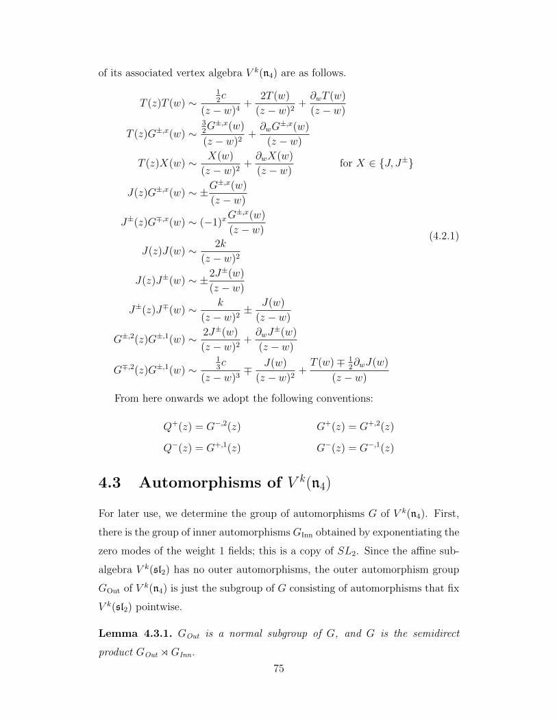
of its associated vertex algebra V k(n4) are as follows.

T (z)T (w) ∼12c

(z − w)4+

2T (w)

(z − w)2+∂wT (w)

(z − w)

T (z)G±,x(w) ∼32G±,x(w)

(z − w)2+∂wG

±,x(w)

(z − w)

T (z)X(w) ∼ X(w)

(z − w)2+∂wX(w)

(z − w)for X ∈ J, J±

J(z)G±,x(w) ∼ ±G±,x(w)

(z − w)

J±(z)G∓,x(w) ∼ (−1)xG±,x(w)

(z − w)

J(z)J(w) ∼ 2k

(z − w)2

J(z)J±(w) ∼ ±2J±(w)

(z − w)

J±(z)J∓(w) ∼ k

(z − w)2± J(w)

(z − w)

G±,2(z)G±,1(w) ∼ 2J±(w)

(z − w)2+∂wJ

±(w)

(z − w)

G∓,2(z)G±,1(w) ∼13c

(z − w)3∓ J(w)

(z − w)2+T (w)∓ 1

2∂wJ(w)

(z − w)

(4.2.1)

From here onwards we adopt the following conventions:

Q+(z) = G−,2(z) G+(z) = G+,2(z)

Q−(z) = G+,1(z) G−(z) = G−,1(z)

4.3 Automorphisms of V k(n4)

For later use, we determine the group of automorphisms G of V k(n4). First,

there is the group of inner automorphisms GInn obtained by exponentiating the

zero modes of the weight 1 fields; this is a copy of SL2. Since the affine sub-

algebra V k(sl2) has no outer automorphisms, the outer automorphism group

GOut of V k(n4) is just the subgroup of G consisting of automorphisms that fix

V k(sl2) pointwise.

Lemma 4.3.1. GOut is a normal subgroup of G, and G is the semidirect

product GOut oGInn.

75

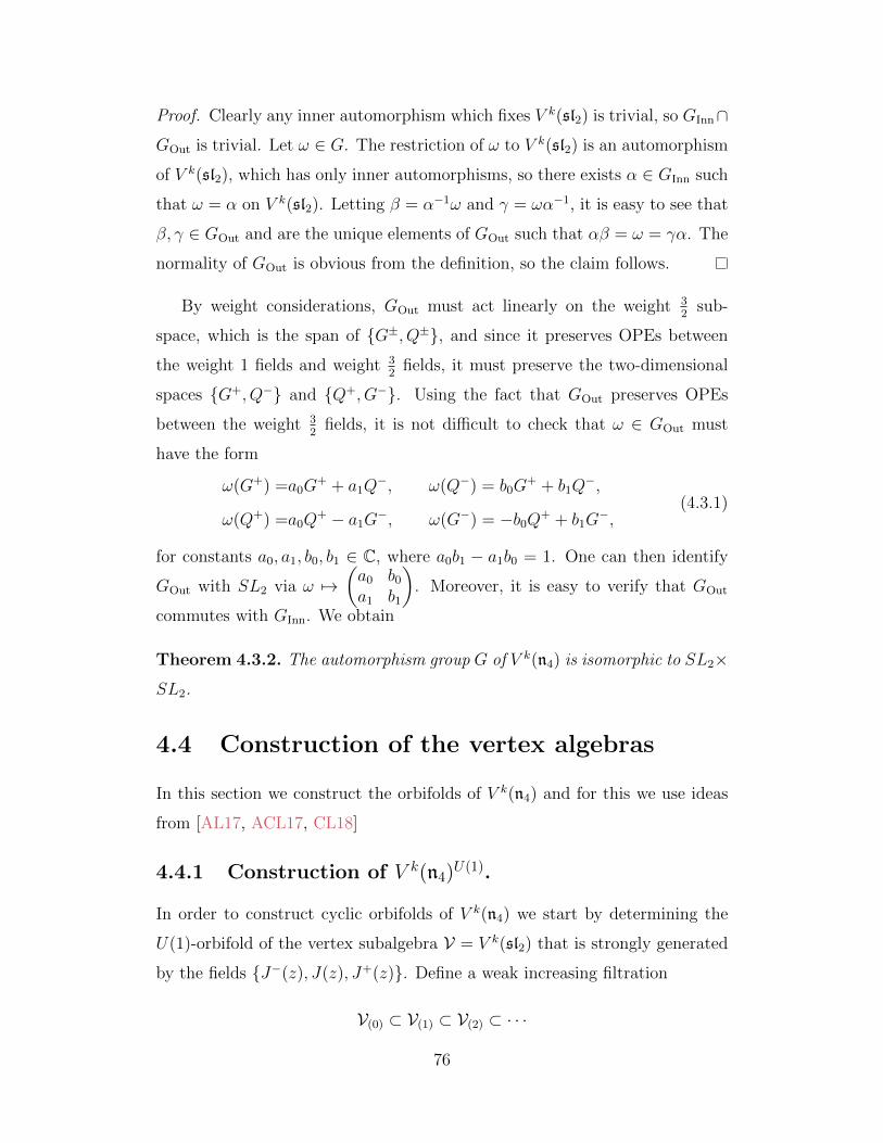
Proof. Clearly any inner automorphism which fixes V k(sl2) is trivial, so GInn∩

GOut is trivial. Let ω ∈ G. The restriction of ω to V k(sl2) is an automorphism

of V k(sl2), which has only inner automorphisms, so there exists α ∈ GInn such

that ω = α on V k(sl2). Letting β = α−1ω and γ = ωα−1, it is easy to see that

β, γ ∈ GOut and are the unique elements of GOut such that αβ = ω = γα. The

normality of GOut is obvious from the definition, so the claim follows.

By weight considerations, GOut must act linearly on the weight 32

sub-

space, which is the span of G±, Q±, and since it preserves OPEs between

the weight 1 fields and weight 32

fields, it must preserve the two-dimensional

spaces G+, Q− and Q+, G−. Using the fact that GOut preserves OPEs

between the weight 32

fields, it is not difficult to check that ω ∈ GOut must

have the form

ω(G+) =a0G+ + a1Q

−, ω(Q−) = b0G+ + b1Q

−,

ω(Q+) =a0Q+ − a1G

−, ω(G−) = −b0Q+ + b1G

−,(4.3.1)

for constants a0, a1, b0, b1 ∈ C, where a0b1 − a1b0 = 1. One can then identify

GOut with SL2 via ω 7→(a0 b0

a1 b1

). Moreover, it is easy to verify that GOut

commutes with GInn. We obtain

Theorem 4.3.2. The automorphism group G of V k(n4) is isomorphic to SL2×

SL2.

4.4 Construction of the vertex algebras

In this section we construct the orbifolds of V k(n4) and for this we use ideas

from [AL17, ACL17, CL18]

4.4.1 Construction of V k(n4)U(1).

In order to construct cyclic orbifolds of V k(n4) we start by determining the

U(1)-orbifold of the vertex subalgebra V = V k(sl2) that is strongly generated

by the fields J−(z), J(z), J+(z). Define a weak increasing filtration

V(0) ⊂ V(1) ⊂ V(2) ⊂ · · ·

76

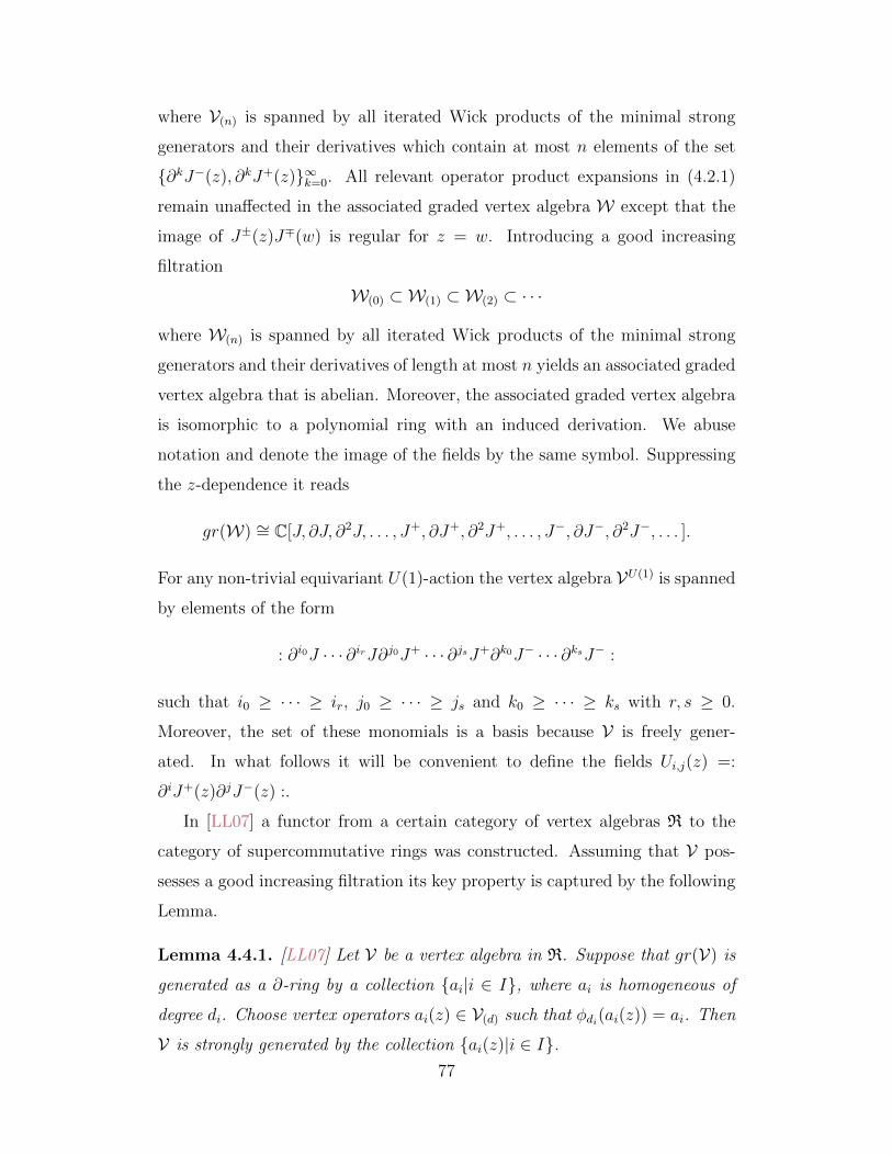
where V(n) is spanned by all iterated Wick products of the minimal strong

generators and their derivatives which contain at most n elements of the set

∂kJ−(z), ∂kJ+(z)∞k=0. All relevant operator product expansions in (4.2.1)

remain unaffected in the associated graded vertex algebra W except that the

image of J±(z)J∓(w) is regular for z = w. Introducing a good increasing

filtration

W(0) ⊂ W(1) ⊂ W(2) ⊂ · · ·

where W(n) is spanned by all iterated Wick products of the minimal strong

generators and their derivatives of length at most n yields an associated graded

vertex algebra that is abelian. Moreover, the associated graded vertex algebra

is isomorphic to a polynomial ring with an induced derivation. We abuse

notation and denote the image of the fields by the same symbol. Suppressing

the z-dependence it reads

gr(W) ∼= C[J, ∂J, ∂2J, . . . , J+, ∂J+, ∂2J+, . . . , J−, ∂J−, ∂2J−, . . . ].

For any non-trivial equivariant U(1)-action the vertex algebra VU(1) is spanned

by elements of the form

: ∂i0J · · · ∂irJ∂j0J+ · · · ∂jsJ+∂k0J− · · · ∂ksJ− :

such that i0 ≥ · · · ≥ ir, j0 ≥ · · · ≥ js and k0 ≥ · · · ≥ ks with r, s ≥ 0.

Moreover, the set of these monomials is a basis because V is freely gener-

ated. In what follows it will be convenient to define the fields Ui,j(z) =:

∂iJ+(z)∂jJ−(z) :.

In [LL07] a functor from a certain category of vertex algebras R to the

category of supercommutative rings was constructed. Assuming that V pos-

sesses a good increasing filtration its key property is captured by the following

Lemma.

Lemma 4.4.1. [LL07] Let V be a vertex algebra in R. Suppose that gr(V) is

generated as a ∂-ring by a collection ai|i ∈ I, where ai is homogeneous of

degree di. Choose vertex operators ai(z) ∈ V(d) such that φdi(ai(z)) = ai. Then

V is strongly generated by the collection ai(z)|i ∈ I.77

This reconstruction property was shown to hold more generally for weak

increasing filtrations (see Lemma 4.1 in [ACL17]).

Lemma 4.4.2. VU(1) is strongly generated by the fields J(z), Un,0(z)∞n=0.

Proof. The weak increasing filtration restricts to the fixed point set

VU(1)(0) ⊂ V

U(1)(1) ⊂ V

U(1)(2) ⊂ · · ·

where VU(1)(i) = VU(1) ∩ V(i). The group action descends to the associated

graded object and we have an isomorphism gr(VU(1)) ∼= WU(1). Likewise, we

have gr(WU(1)) ∼= gr(W)U(1). For the latter the generating set of fields as a

∂-ring is given by J, ua,b∞a,b=0 where ua,b = ∂aJ+∂bJ−. The vertex algebra

WU(1) is an object in R. By the previous Lemma it is strongly generated

by J(z), Ua,b(z)∞a,b=0 where Ua,b(z) =: ∂aJ+(z)∂bJ−(z) :. Since the Lemma

also holds for weak increasing filtrations and the map gr is equivariant with

respect to the group action up to isomorphism we can repeat this argument

to obtain a strongly generating set of VU(1). Therefore, and by making use of

the Leibniz rule, VU(1) is strongly generated by J(z), Ua,0(z)∞a=0

Lemma 4.4.2 can be improved upon. The proof made use of the vertex

algebra gr(W)U(1) which is strongly generated by J, ua,b∞a,b=0. Note that due

to commutativity there exist identities between these generators

ua,buc,d = ua,duc,b.

We will show that a preimage of ua,buc,d − ua,duc,b in VU(1) does not vanish,

thereby showing the existence of relations between generators. From here

onwards any z-dependence of the fields will be suppressed for easier readability.

Considering conformal weight and Lemma 4.4.2 it follows that

: Ua,bUc,d − Ua,dUc,b := cNUN,0 + f(J, U0,0, . . . , UN−1,0)

for some scalar cN where a + b + c + d + 2 = N and f is a sum of normally

ordered products in the strong generators of conformal weight less than N + 2

78

and their derivatives. Invoking the Leibniz rule yields the identity Ua,b =∑bi=0(−1)i

(bi

)∂b−iUa+i,0 which implies that the last equality can be rewritten

cNUN,0 = g(J, U0,0, . . . , UN−1,0)

where g is again a normally ordered polynomial in the strong generators of

conformal weight less thanN+2 and their derivatives. This shows that the field

UN,0 can be written as a normally ordered polynomial in strong generators of

lower conformal weight, provided that cN does not vanish. Following [ACL17]

we will refer to such an expression as a decoupling relation. What follows

are two technical Lemmas which will serve as a preparation for the proof of

Proposition 4.4.6.

For some n ∈ N we may write a given element ω ∈ VU(1)(2) of conformal

weight n+ 2 as a sum of normally ordered products gω(J, U0,0, . . . , Un,0) in the

strong generators of conformal weight at most n+2 and their derivatives. Such

a normally ordered product is not unique due to the existence of decoupling

relations and different conventions for normal ordering. Let the coefficient of

: ∂n−iJ+∂iJ− : in gω be denoted by cn,i(ω) and define

cn(ω) =n∑i=0

(−1)icn,i(ω).

Lemma 4.4.3. For any ω ∈ VU(1)(2) of weight n+ 5 for n ∈ N the coefficient of

Un+3,0 appearing in gω is independent of all choices of normal orderings and

is equal to cn(ω).

Proof. The proof is analogous to the proof of Lemma 5.2 in [ACL17].

Remark 4.4.4. Note that we use strong generators of the form Un,0 (cf. loc.

cit.). We may simply rewrite these by using the Leibniz rule as above with

their difference being a total derivative. The factor (−1)n does not appear in

our case because of the different choice in strong generators.

Lemma 4.4.5. Let n ∈ N0 and let Pm denote a sum of normally ordered prod-

ucts of strong generators of VU(1) of weight less than m and their derivatives.

: U0,0U1,n :=

(2

n+ 2+

k

n+ 2

)U1,n+2 −

1

n+ 1U2,n+1+

79

+

(1 +

k

3

)U3,n +

2

(n+ 1)(n+ 2)(n+ 3)Un+3,0 + Pn+5

: U0,nU1,0 :=( 2

n+ 2+k

2

)U1,n+2 − U2,n+1+

+

2

(n+ 1)(n+ 2)(n+ 3)+ (−1)n

( 1

n+ 1+

k

n+ 3

)Un+3,0 + Pn+5

Proof. The proof is a straightforward computation using only the definition of

normal ordering and the commutation relations of sl2 at level k.

Proposition 4.4.6. For any non-vanishing level k the vertex algebra V k(sl2)U(1)

is of type W(1, 2, 3, 4, 5). A set of minimal strong generators is J, Un,03n=0.

Proof. Since all strong generators of VU(1) have a different conformal weight

by Lemma 4.4.2 and the smallest non-trivial identity between the strong gen-

erators of gr(W)U(1) is u0,0u1,1 = u0,1u1,0 we will focus on a one-parameter

family of decoupling relations that involve the expression

ωndef=: U0,0U1,n − U0,nU1,0 :

for n ∈ N. Note that the non-regular part of the OPE of J±(z)J∓(w) does not

contain the field J+(z) or J−(z) and therefore ωn ∈ VU(1)(2) . The element ωn can

be written as a sum of normally ordered products in the strong generators of

VU(1) and their derivatives. The coefficient of Un+3,0 is canonical in the sense

of Lemma 4.4.3. Due to Lemma 4.4.5 it can be easily computed and equals

cn+3(ωn) = (−1)n+1kn(n+ 5)

6(n+ 2)(n+ 3).

This shows existence of a decoupling relation for Un+4,0 for all n ∈ N0 at any

non-vanishing level k. Hence, V k(sl2)U(1) is strongly generated by J, Un,03n=0

for k 6= 0. That there exists no further decoupling relation between the re-

maining strong generators can be checked directly and implies minimality of

the set.

Remark 4.4.7. It is easy to find a maximal subset of minimal strong genera-

tors which have no non-regular OPEs with the Heisenberg field. By the identity

V k(sl2)U(1) = H⊗Com(H, V k(sl2)) this is another proof that Com(H, V k(sl2))

is of type W(2, 3, 4, 5) which was initially proven in [DW10].

80

The last Proposition can be used to prove a similar statement about V k(n2)U(1).

It will be convenient to introduce the following fields

Va,bdef=: ∂aG+∂bG− : .

Proposition 4.4.8. For any level k 6= 0,−2 the vertex algebra V k(n2)U(1) is

of type W(1, 2, 3, 4, 5). A set of minimal strong generators is J, T, Vn,02n=0.

Proof. Denote the standard strong generators of V k(sl2) by H,X± and let E

be the bc-system of rank 1. Considering the tensor product V k(sl2)⊗E we will

abuse notation and denote the strong generators by the same symbols. Let

K = 12H− : bc :. The zero mode K0 integrates to a U(1)-action on V k(sl2)⊗E .

Lemma 8.6 in [CL19] shows that if k 6= −2 then

V `(n2) ∼= Com(H1, Vk(sl2)⊗ E) (4.4.1)

with central charge 3kk+2

where H1 is the Heisenberg vertex algebra generated

by K. The zero mode H0 integrates to a U(1)-action as well. Denote the

group associated to the zero mode of K (H) by G1 (G2) and let H2 be the

Heisenberg vertex algebra generated by H.

H1 ⊗ V `(n2)G2 ∼=((V k(sl2)⊗ E)G2

)G1

∼= (H2 ⊗ Com(H2, Vk(sl2)⊗ E))G1

∼= H2 ⊗ Com(H2, Vk(sl2))⊗ EG1

The commutativity of the two group actions was used in the first equality. All

G1-invariant fields in E can be strongly generated by the fields : ∂ib∂jc : for

i, j ≥ 0. By the action of the derivation a set of strong generators is given by

: ∂ibc :∞i=0. It is easy to show that the equality

: (: ∂nbc :)(: bc :) :=n+ 2

n+ 1: ∂n+1bc : +∂ω

holds for n ≥ 0 where ω is a linear combination of the fields ∂n−i : ∂ibc : for

i = 0, . . . , n. This implies that : bc : strongly generates EG1 . From the above

isomorphism one can deduce

V `(n2)G2 ∼= Com(H1,H2 ⊗ Com(H2, Vk(sl2))⊗ EG1).

81

It now follows from Proposition 4.4.6 that the only strong generator of weight

1 is an element of the commutant Com(H1,H2 ⊗ EG1) which is isomorphic to

a Heisenberg vertex algebra. Hence, V k(n2)G2 is of type W(1, 2, 3, 4, 5). The

Heisenberg and the Virasoro field of V k(n2) are elements of the kernel of H0.

The isomorphism in (4.4.1) for the weight 32

fields is given by

: X±b : 7→ δ±G± where δ+δ− = 2 + k.

From the action of the zero mode H0 it is immediate that a set of strong

generators of V k(n2)G2 of weight 3, 4 and 5 can be given by Vn,02n=0.

We now shift our focus towards V k(n4)U(1). Let J+ and G+ be in identical

U(1)-representations ρi for i = 1, 2. The group action on V k(n4) will be chosen

to be such that it restricts to (and is compatible with) ρ1 and ρ2. All strong

generators on which the group action is left undetermined by this requirement

are chosen to be in the trivial representation. Note that restricting to Z/2Z at

level k = 1 yields the automorphism on H0(X,ΩCdR) on a K3 surface X that

is induced from a fixed point free involution as mentioned in the introduction.

The vertex algebras from Proposition 4.4.6 and 4.4.8 are vertex subalgebras

of V k(n4)U(1). Their minimal strong generators are part of the set of strong

generators of V k(n4)U(1). In contrast to before there exists a decoupling re-

lation for U3,0 for all non-vanishing levels k (see (A.1.1)). All other strong

generators of the two vertex subalgebras are part of the minimal set of strong

generators of V k(n4)U(1) which follows from the OPEs in (4.2.1). The proof of

the following Lemma is a straightforward computation and will be omitted.

Lemma 4.4.9. Let Pm be a sum of normally ordered products of weight m

such that each summand includes the field ∂iT or ∂jJ , and at most one field

∂kVl,0 for some i, j, k, l,m ∈ N0. Let n ∈ N0.

k(6 + n)

3(3 + n)Vn+3,0 = : V0,0Vn,0 : +k∂Vn+2,0 −

(1

2 + 2n+ k

)∂2Vn+1,0 +

k

3∂3Vn,0 + Pn+6

The last Lemma now implies that the union of the sets of minimal strong

generators of the subalgebras V (sl2)U(1) and V (n2)U(1) yields a set of even

minimal strong generators of V (n4)U(1). All possible homogeneous minimal odd

82

generators (up to sums of normally ordered products of fields of lower weight)

necessarily are in the linear span of the fields in the set Q+, Q−, An,0, Bn,0∞n=0

where we define

An,0def=: ∂nJ+G− : and Bn,0

def=: ∂nJ−G+ :

for n ∈ N0. The proof of the following Lemma is again a straightforward

computation and will be omitted.

Lemma 4.4.10. Let n ∈ N0 and let Pm be a sum of normally ordered products

of strong generators of V k(n4)U(1) of weight less than m and their derivatives.

nk

2(n+ 2)An+2,0 + Pn+ 9

2= : Un,0A0,0 : − : U0,0An,0 : + : (Un+1,0 − ∂Un,0)Q− :

− 1

n+ 1

n+1∑i=0

(−1)i(n

i

): ∂iUn+1−i,0Q

− :

nk

2(n+ 2)Bn+2,0 + Pn+ 9

2=

n∑i=0

(−1)i(n

i

): ∂iUn−i,0B0,0 : + : ∂iUn+1−i,0Q

+ :

− 1

n+ 1: Un+1,0Q

+ : +(−1)n+1 : U0Bn,0 :

The last Lemma shows the existence of decoupling relations for the fields

in the set Ai,0, Bi,0∞i=3. As before it can be checked directly that there are

no decoupling relations for the remaining strong generators. Hence, this yields

the following.

Theorem 4.4.11. For any level k 6= −2, 0 the vertex algebra V k(n4)U(1) is

of type W(1, 32

2, 22, 5

2

2, 32, 7

2

2, 42, 9

2

2, 5). A set of minimal strong generators is

given by J,Q±, T, Ui,0, Ai,0, Bi,0, Vi,02i=0.

4.5 Construction of the cyclic orbifold

Let U(n4)G be the universal enveloping algebra of n4 that is invariant under the

group G. From here onwards we will restrict the group to be cyclic G ∼= Z/NZ.

By section 4.2.3 there are isomorphisms

N−1⊕i=0

Ci ⊗Wi∼= V k(n4) ∼=

∞⊕i=−∞

Ci ⊗ Vi

83

as a (Z/NZ,U(n4)Z/NZ)-module and as a (U(1),U(n4)U(1))-module, respec-

tively. By restriction this leads to an isomorphism

Wa∼=

∞⊕k=−∞

VkN+a

for a = 0, . . . , N − 1 as a U(n4)Z/NZ-module.

It will be convenient to define the following fields

Y (σ(i)±a1,...,ajN

, z) = Σ(i)±a1,...,ajN

def=: ∂a1J± · · · ∂ajN−iJ±∂ajN−i+1G± · · · ∂ajNG± :

for i = 0, . . . , jN and ai ∈ N0.

Lemma 4.5.1. The vertex algebra V k(n4)Z/NZ is strongly generated by the

strong generators of V k(n4)U(1) and the fields Σ(i)±a1,...,aN for i = 0, . . . , N and

a1, . . . , aN ≥ 0.

Proof. Let V± =⊕

j∈N V±jN and let i = 0, . . . , N . Each vector space VjN

for j ∈ Z\0 is a U(n4)U(1)-module and generated by the vectors in the set

σ(i)+a1,...,ajN∞a1,...,ajN=0. The vertex algebra on the vector space V 0⊕V+ is induced

from V k(n4). Due to commutativity of the fields in the set Σ(i)+a1,...,aNNi=0 the

vertex algebra is strongly generated by these fields and the strong generators of

V 0. By the same argument the vertex algebra over the vector space V 0 ⊕ V−is strongly generated by the fields in the set Σ(i)−

a1,...,aNNi=0 and the strong

generators of V 0. Observe that the fields that appear in the OPEs between

the strong generators in VN and V−N are necessarily elements of V 0. This

proves the proposition.

Some fields will be superfluous as strong generators due to the action of

the derivation d. The generating function of the fields Σ(l)±a1,...,aN for fixed l

with respect to weight will show which of these can be neglected as strong

generators. It can be obtained by a simple counting argument.

Lemma 4.5.2. The generating function for the number of fields Σ(l)±a1,...,aN with

respect to conformal weight is

qN+ l2

2

N−l∏i=1

1

1− qil∏

j=1

1

1− qj.

84

Proof. The weight of the field Σ(l)±a1,...,aN equals N + 1

2l + a + b where a =∑N−l

i=1 ai and b =∑N

i=N−l+1 ai. Due to (anti-)commutativity of the fields in

the set ∂iJ+, ∂iG+∞i=0 the number of fields at a given weight is determined

by the number of partitions of a with at most N − l parts and the number

of partitions of b with exactly l and with exactly l − 1 parts such that all

summands are distinct in both cases. The latter condition exists since at

most one of the coefficients in the set aN−i+1, . . . , aN can be zero, otherwise

Σ(i)±a1,...,aN vanishes.

Let V(l) be the subspace of the Fock space of V k(n4) spanned by the vectors

in the set σ(l)±a1,...,aN∞a1,...,aN=0. It is obvious that d ∈ Der(V(l)) and that it

increases the conformal weight by 1. It follows that there are decoupling

relations for vectors in the spanning set of V(l) when taking the action of the

derivation into account. Dropping vectors in the set σ(l)±a1,...,aN∞a1,...,aN=0 which

decouple for this reason amounts to multiplying the generating function from

Lemma 4.5.2 by (1− q).

We will now focus on the case N = 2. Multiplying the generating function

from the previous Lemma by (1− q) yields

l = 0 :∞∑i=0

q2n+2 , l = 1 :∞∑i=0

qn+ 52 , l = 2 :

∞∑i=0

q2n+4.

Thus, Lemma 4.5.1 can be improved upon as a set of strong generators of

V k(n4)Z/2Z can be given by the strong generators of Vk(n4)U(1) and the fields

in the set

Σ(0)±2n,0 ,Σ

(1)±n,0 ,Σ

(2)±2n+1,0∞n=0. The following Lemma will set up the proof of The-

orem 4.5.4.

Lemma 4.5.3. Let n ∈ N and c(i)n , d

(i)n ∈ Q for i = 0, 1, 2.

: U2n,0Σ(0)+0,0 − U0,0Σ

(0)+2n,0 : = p(0)

n (k) Σ(0)+2n+2,0 +

2n∑i=0

c(0)i : ∂iHΣ

(0)+2n−i,0 :

: U2n−1,0Σ(0)+1,0 − U0,0Σ

(0)+2n−1,1 : = q(0)

n (k) Σ(0)+2n+2,0 +

2n∑i=0

d(0)i : ∂iHΣ

(0)+2n−i,0 :

: Σ(0)+n,0 B0,0 − Un,0Σ

(1)+0,0 + Σ

(0)+n+1,0Q

+ : = p(1)n (k) Σ

(1)+n+2,0 +

n+1∑i=0

c(1)i : ∂iHΣ

(1)+n+1−i,0 :

85

: Σ(0)+n,0 B0,0 − U0,0Σ

(1)+n,0 + Σ

(0)+n,1 Q+ : = q(1)

n (k) Σ(1)+n+2,0 +

n+1∑i=0

d(1)i : ∂iHΣ

(1)+n+1−i,0 :

: B0,0Σ(1)+2n−1,0 − Σ

(1)+2n−1,1Q

+ : = p(2)n (k) Σ

(2)+2n+1,0 +

2n∑i=0

c(2)i : ∂iHΣ

(2)+2n−i,0 :

: B2n−1,0Σ(1)+0,0 +

1

2nΣ

(1)+0,2nQ

+ : = q(2)n (k) Σ

(2)+2n+1,0 +

2n∑i=0

d(2)i : ∂iHΣ

(2)+2n−i,0 :

p(0)n (k) = −

8n

2n+ 1+

n

2n+ 2k q

(0)n (k) =

4

3+

7 + 2n

6(2n+ 1)k

p(1)n (k) =

2

n+ 2

[(n−

1 + (−1)n

n+ 1

)+ (−1)n

k

2

]q(1)n (k) =

1

n+ 2

[(−1)

n+ 1[4n+ 5 + (−1)n+1(2n+ 1)] +

k

2[n+ 2(−1)n]

]p

(2)n (k) =

2 + k

2n+ 1q(2)n (k) =

2− k2n+ 1

Proof. Computing the left hand side of each of these equations is straightfor-

ward and leads directly to the right hand side by using only the definition of

normal ordering and the commutation relations of n4 which are equivalent to

the OPEs as stated in (4.2.1).

Theorem 4.5.4. Let k 6= −2, 0, 4, 16. The vertex algebra V k(n4)Z/2Z is of type

W(1, 32

2, 24, 5

2

4, 32, 7

2

4, 45). A set of minimal strong generators is

S = H,Q±, T, Ui,0, Ai,0, Bi,0, Vi,0,Σ(i)±0,0 ,Σ

(0)±2,0 ,Σ

(1)±1,0 ,Σ

(2)±1,0 1

i=0.

At level k = 4 a set of minimal strong generators is S ∪ Σ(1)±2,0 . At level

k = 16 a set of minimal strong generators is S ∪ U2,0, A2,0, B2,0.

Proof. By Lemma 4.5.1 and the discussion thereafter the vertex algebra V k(n4)Z/2Z

is strongly generated by the strong generators of V k(n4)U(1) and the fields in the

set Σ(0)±2n,0 ,Σ

(1)±n,0 ,Σ

(2)±2n+1,0∞n=0. Observe in Lemma 4.5.3 that for any i ∈ 0, 1, 2

the roots of p(i)n and q

(i)n are distinct for all n ∈ N. It follows that the fields

Σ(0)+2n+4,0,Σ

(1)+n+3,0,Σ

(2)+2n+3,0∞n=0 decouple at any level k. Let θ ∈ Aut(V k(n4)) such

that it restricts to an involution on the strong generators of V k(sl2) given by

θ(J+) = J− , θ(J) = −J , θ(J−) = J+

and such that θ(G+) = G−. These requirements fix the action on the remaining

strong generators. The map θ is an automorphism of V k(n4)Z/2Z a fortiori

86

and acting on the decoupling relations of Lemma 4.5.3 shows that the fields

Σ(0)−2n+4,0,Σ

(1)−n+3,0,Σ

(2)−2n+3,0∞n=0 decouple at any level k as well. The existence

of decoupling relations for all remaining strong generators can be checked

directly.2 The field Σ(1)+2,0 decouples at all levels k 6= 4 (see (A.1.2)). Acting

on the decoupling relation of Σ(1)+2,0 with the automorphism θ shows that Σ

(1)+2,0

also decouples at all levels k 6= 4. Furthermore, the fields U2,0, A2,0 and B2,0

decouple at all levels k 6= 16 (see (A.1.3)-(A.1.5)) and V2,0 decouples at all

levels k 6= 0 (see (A.1.6) and (A.1.7)). These exhaust all decoupling relations

for the minimal strong generators which proves the Theorem.

4.6 Structure of the vertex algebras

We will now look at sub-structures and simple quotients of the two orbifolds

of V k(n4) that were constructed in the previous section. It will be helpful to

define the following: Let Ri ∈ V k(n4) be a field and define

Ci = Q+ 0 Ri , Di = −Q− 0 R

i , Si =1

2

(Q− 0 C

i +Q+ 0 Di).

It is immediate that the fields in the set S i = Ri, Ci, Di, Si and their deriva-

tives span a V k(n2)-module. Taking R0 = H and Ri+1 = Ui,0 for i = 0, 1, 2

it can be checked that the fields in the set S = S i3i=0 strongly generate

V k(n4)U(1) at all levels k 6= 0,−2 (cf. Theorem 4.4.11). Furthermore, taking

R3 = Σ(0)+0,0 and R4 = Σ

(1)+1,0 as well as Rn+2 = θ(Rn) for n = 3, 4 with θ

being the automorphism defined in the proof of Theorem 4.5.4 we see that

the set S i6i=0 contains all minimal strong generators of V k(n4)Z/2Z at levels

k 6= −2, 0, 4, 16 (cf. Theorem 4.5.4).

Theorem 4.6.1. Let k 6= 0,−2. For all but finitely many levels k the simple

quotient of V k(n4)U(1) is of type W(1, 32

2, 22, 5

2

2, 32, 7

2

2, 42, 9

2

2, 5). The full list

of exceptions is stated in the following table.

2In our case this was done using Thielemans’ MathematicaTMpackage [Thi91].

87

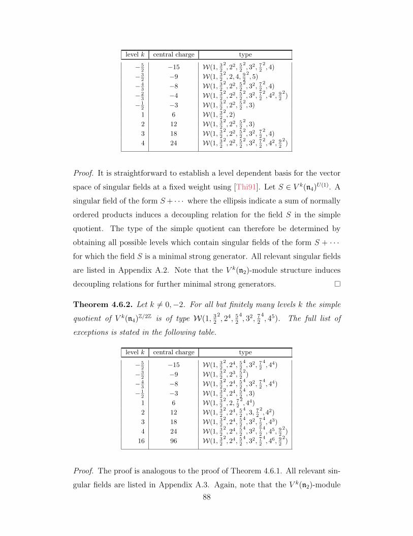
level k central charge type

− 52 −15 W(1, 32

2, 22, 52

2, 32, 72

2, 4)

− 32 −9 W(1, 32

2, 2, 4, 92

2, 5)

− 43 −8 W(1, 32

2, 22, 52

2, 32, 72

2, 4)

− 23 −4 W(1, 32

2, 22, 52

2, 32, 72

2, 42, 92

2)

− 12 −3 W(1, 32

2, 22, 52

2, 3)

1 6 W(1, 322, 2)

2 12 W(1, 322, 22, 52

2, 3)

3 18 W(1, 322, 22, 52

2, 32, 72

2, 4)

4 24 W(1, 322, 22, 52

2, 32, 72

2, 42, 92

2)

Proof. It is straightforward to establish a level dependent basis for the vector

space of singular fields at a fixed weight using [Thi91]. Let S ∈ V k(n4)U(1). A

singular field of the form S+ · · · where the ellipsis indicate a sum of normally

ordered products induces a decoupling relation for the field S in the simple

quotient. The type of the simple quotient can therefore be determined by

obtaining all possible levels which contain singular fields of the form S + · · ·

for which the field S is a minimal strong generator. All relevant singular fields

are listed in Appendix A.2. Note that the V k(n2)-module structure induces

decoupling relations for further minimal strong generators.

Theorem 4.6.2. Let k 6= 0,−2. For all but finitely many levels k the simple

quotient of V k(n4)Z/2Z is of type W(1, 32

2, 24, 5

2

4, 32, 7

2

4, 45). The full list of

exceptions is stated in the following table.

level k central charge type

− 52 −15 W(1, 32

2, 24, 52

4, 32, 72

4, 44)

− 32 −9 W(1, 32

2, 23, 52

2)

− 43 −8 W(1, 32

2, 24, 52

4, 32, 72

4, 44)

− 12 −3 W(1, 32

2, 24, 52

4, 3)

1 6 W(1, 322, 2, 72

2, 44)

2 12 W(1, 322, 24, 52

4, 3, 72

2, 42)

3 18 W(1, 322, 24, 52

4, 32, 72

4, 43)

4 24 W(1, 322, 24, 52

4, 32, 72

4, 45, 92

2)

16 96 W(1, 322, 24, 52

4, 32, 72

4, 46, 92

2)

Proof. The proof is analogous to the proof of Theorem 4.6.1. All relevant sin-

gular fields are listed in Appendix A.3. Again, note that the V k(n2)-module

88

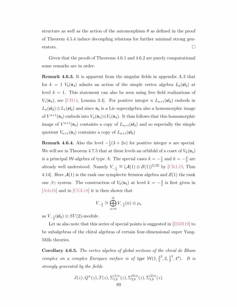
structure as well as the action of the automorphism θ as defined in the proof

of Theorem 4.5.4 induce decoupling relations for further minimal strong gen-

erators.

Given that the proofs of Theorems 4.6.1 and 4.6.2 are purely computational

some remarks are in order:

Remark 4.6.3. It is apparent from the singular fields in appendix A.3 that

for k = 1 Vk(n4) admits an action of the simple vertex algebra Lk(sl2) at

level k = 1. This statement can also be seen using free field realizations of

V1(n4), see [CH14, Lemma 3.4]. For positive integer n Ln+1(sl2) embeds in

Ln(sl2)⊗L1(sl2) and since n4 is a Lie superalgebra also a homomorphic image

of V n+1(n4) embeds into Vn(n4)⊗V1(n4). It thus follows that this homomorphic

image of V n+1(n4) containts a copy of Ln+1(sl2) and so especially the simple

quotient Vn+1(n4) containts a copy of Ln+1(sl2)

Remark 4.6.4. Also the level −12(3 + 2n) for positive integer n are special.

We will see in Theorem 4.7.5 that at these levels an orbifold of a coset of Vk(n4)

is a principal W-algebra of type A. The special cases k = −12

and k = −32

are

already well understood. Namely V− 12

∼= (A(1) ⊗ S(1))Z/2Z by [CKL19, Thm

4.14]. Here A(1) is the rank one symplectic fermion algebra and S(1) the rank

one βγ system. The construction of Vk(n4) at level k = −32

is first given in

[Ada16] and in [CGL18] it is then shown that

V− 32

∼=∞⊕n=0

V− 32(n)⊗ ρn

as V− 32(sl2)⊗ SU(2)-module.

Let us also note that this series of special points is suggested in [BMR19] to

be subalgebras of the chiral algebras of certain four-dimensional super Yang-

Mills theories.

Corollary 4.6.5. The vertex algebra of global sections of the chiral de Rham

complex on a complex Enriques surface is of type W(1, 32

2, 2, 7

2

2, 44). It is

strongly generated by the fields

J(z), Q±(z), T (z),Σ(1)±1,0 (z),Σ

(0)±2,0 (z),Σ

(2)±1,0 (z).

89

4.7 Coset of V k(n4) by its affine subalgebra

In this section, we study the coset

Ck = Com(V k(sl2), V k(n4)), (4.7.1)

and we regard V k(n4) as an extension of V k(sl2) ⊗ Ck. In Theorem 5.4 of

[ACKL17], Ck was incorrectly stated to be of type W(2, 33, 4, 53, 6, 73, 8). In

this section, we give the correct description as well as some more details about

its structure.

As in Section 4 of [ACKL17], if we rescale the generators of V k(n4) by 1√k,

there is a well-defined limit as k →∞, and

limk→∞

V k(n4) ∼= H(3)⊗ T ⊗ Godd(4).

In this notation, H(3) is the rank 3 Heisenberg vertex algebra, T is a

generalized free field algebra with one even generator T satisfying T (z)T (w) ∼

6(z−w)−4, and Godd(4) is the generalized free field algebra with odd generators

G±, Q± satisfying

G+(z)G−(w) ∼ 2(z − w)−3, Q+(z)Q−(w) ∼ 2(z − w)−3.

Note that our normalizations of the generator differ slightly from those in

[ACKL17], but this does not change the above result. Note that the action of

the inner automorphism group GInn∼= SL2 on V k(n4) coming from integrating

the zero-mode action of sl2 gives rise to action of SL2 on Godd(4), such that

G+, Q+ and G−, Q− both transform as copies of the standard module C2.

As shown in [ACKL17] right before Theorem 4.12, Ck has a well-defined

limit as k →∞, and

limk→∞Ck ∼= T ⊗

(Godd(4)

)SL2 .

Moreover, structure of(Godd(4)

)SL2 can be worked out using classical invariant

theory. First, we have the infinite generating set

mj = : G+∂jQ+ : + : ∂jG+Q+ :,

pj = : G−∂jQ− : + : ∂jG−Q− :,

wj = : G+∂jG− : + : Q+∂jQ− : .

(4.7.2)

90

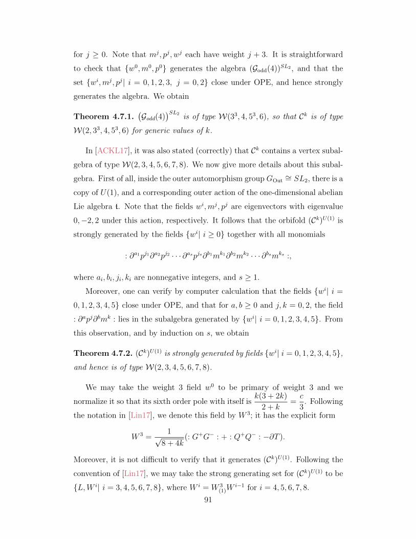
for j ≥ 0. Note that mj, pj, wj each have weight j + 3. It is straightforward

to check that w0,m0, p0 generates the algebra (Godd(4))SL2 , and that the

set wi,mj, pj| i = 0, 1, 2, 3, j = 0, 2 close under OPE, and hence strongly

generates the algebra. We obtain

Theorem 4.7.1.(Godd(4)

)SL2 is of type W(33, 4, 53, 6), so that Ck is of type

W(2, 33, 4, 53, 6) for generic values of k.

In [ACKL17], it was also stated (correctly) that Ck contains a vertex subal-

gebra of type W(2, 3, 4, 5, 6, 7, 8). We now give more details about this subal-

gebra. First of all, inside the outer automorphism group GOut∼= SL2, there is a

copy of U(1), and a corresponding outer action of the one-dimensional abelian

Lie algebra t. Note that the fields wi,mj, pj are eigenvectors with eigenvalue

0,−2, 2 under this action, respectively. It follows that the orbifold (Ck)U(1) is

strongly generated by the fields wi| i ≥ 0 together with all monomials

: ∂a1pj1∂a2pj2 · · · ∂aspjs∂b1mk1∂b2mk2 · · · ∂bsmks :,

where ai, bi, ji, ki are nonnegative integers, and s ≥ 1.

Moreover, one can verify by computer calculation that the fields wi| i =

0, 1, 2, 3, 4, 5 close under OPE, and that for a, b ≥ 0 and j, k = 0, 2, the field

: ∂apj∂bmk : lies in the subalgebra generated by wi| i = 0, 1, 2, 3, 4, 5. From

this observation, and by induction on s, we obtain

Theorem 4.7.2. (Ck)U(1) is strongly generated by fields wi| i = 0, 1, 2, 3, 4, 5,

and hence is of type W(2, 3, 4, 5, 6, 7, 8).

We may take the weight 3 field w0 to be primary of weight 3 and we

normalize it so that its sixth order pole with itself isk(3 + 2k)

2 + k=c

3. Following

the notation in [Lin17], we denote this field by W 3; it has the explicit form

W 3 =1√

8 + 4k(: G+G− : + : Q+Q− : −∂T ).

Moreover, it is not difficult to verify that it generates (Ck)U(1). Following the

convention of [Lin17], we may take the strong generating set for (Ck)U(1) to be

L,W i| i = 3, 4, 5, 6, 7, 8, where W i = W 3(1)W

i−1 for i = 4, 5, 6, 7, 8.

91

It is readily verified that the hypotheses of Theorem 6.4 of [Lin17] are

satisfied, so that (Ck)U(1) can be realized as a quotient of W(c, λ) of the form

WI(c, λ) = WI(c, λ)/I. In this notation, I ⊆ C[c, λ] is some prime ideal in

the ring of parameters C[c, λ], and I is the maximal proper graded ideal of

WI(c, λ) =W(c, λ)/I · WI(c, λ).

By computing the third order pole of W 3 with itself, it is straightforward

to verify that I is the ideal (λ + 116

). Rather surprisingly, this same vertex

algebra was studied in Section 11 of [Lin17]. Combining this calculation with

Corollary 10.3 of [Lin17], We obtain

Theorem 4.7.3. (Ck)U(1) is isomorphic to the coset

Com(V `(sl2), V `+1(sl2)⊗W−5/2(sl4, frect)),

where the parameters k and ` are related by k = −`+ 1

`+ 2.

Remark 4.7.4. This Theorem nicely relates to the coset realization of V k(n4)

of [CFL19]. Let V k(n) denote the irreducible highest-weight module of sl2 of

highest weight nω at level k. ω is the fundamental weight of sl2 and ρm denotes

the irreducible highest-weight module of SU(2) of highest weight mω. Also

let n be equal to 0 of n is even and 1 otherwise. We have the following list of

isomorphisms

1. In [CKLR19, Section 5] diagonal Heisenberg cosets of rank n βγ sys-

tem times rank m bc system where studied. These cosets were denoted

by C(n,m) and C(2, 0) ∼= W−5/2(sl4, frect) [CKLR19, Remark 5.3] and

C(2, 2) ∼= L1(sl(2|2)) [CKLR19, Theorem 5.5]. Moreover C(0, 2) is noth-

ing but the lattice VOA L1(sl2) and so we have that W−5/2(sl4, frect) ⊂

Com (L1(sl2), L1(sl(2|2))) and by passing to the simple quotient L1(psl(2|2))

of L1(sl(2|2)) we also haveW−5/2(sl4, frect) ⊂ Com (L1(sl2), L1(psl(2|2))).

The branching rules [Cre17, Cor. 5.3] and [CG17, Rem. 9.11]

W−5/2(sl4, frect) ∼=∞⊕n=0

V −1(2m) (4.7.3)

and

L1(psl(2|2)) ∼=∞⊕n=0

V −1(n)⊗ ρn ⊗ L1(n)

92

tell us that

W−5/2(sl4, frect) ∼= Com (L1(sl2), L1(psl(2|2)))U(1) .

2. In [CFL19] a vertex superalgebra Y (λ) that is very closely related to

L1(d(2, 1;−λ))⊗ L1(psl(2|2)) has been constructed. It satisfies

Y (λ)Z/2Z ∼= Com (L1(sl2 ⊗ L1(sl2, L1(d(2, 1;−λ))⊗ L1(psl(2|2))) .

3. Y (λ) decomposes

Y (λ) :=∞⊕

n,m=0

V k1(n)⊗ V k2(n)⊗ V −1(m)⊗ ρm

as V k1(sl2)⊗V k2(sl2)⊗V −1(sl2)⊗SU(2)-module for generic complex λ.

Here k1 = λ−1 − 1, k2 = λ− 1. Then by [CFL19] and for irrational λ we

have that

V k2(n4) ∼= Com(V k1−1(sl2), Y (λ)

).

4. Putting all these together we get

(Ck2)U(1) ∼= Com(V k2 ⊗ V k1−1(sl2), Y (λ)

)U(1)

∼= Com

(V k2 ⊗ V k1−1(sl2),

∞⊕n,m=0

V k1(n)⊗ V k2(n)⊗ V −1(m)⊗ ρm)

)U(1)

∼= Com

(V k1−1(sl2),

∞⊕m=0

V k1(sl2)⊗ V −1(m)⊗ ρm)

)U(1)

∼= Com

(V k1−1(sl2),

∞⊕m=0

V k1(sl2)⊗ V −1(2m))

).

which using (4.7.3) and noticing that k2 = − k1

k1+1nicely compares to the

Theorem.

We now present some consequences of the identification of (Ck)U(1) with a

quotient of W(c, λ). Recall from Section 10 of [Lin17], we can obtain coin-

cidences between the simple quotient of (Ck)U(1) with various other algebras

arising as quotients ofW(c, λ) by finding the intersection points on their trun-

cation curves.

93

Recall that if we regard Ck as a one-parameter vertex algebra, with k a

formal variable, the specialization of Ck at a complex number k = k0 need not

coincide with the actual coset, but this can only fail when k0 + 2 ∈ Q≤0. This

property is inherited by the orbifold (Ck)U(1) if we also omit the point k0 = 0.

By abuse of notation, in the results below, (Ck0)U(1) will always refer to the

specialization of the one-parameter vertex algebra (Ck)U(1) at the point k = k0,

even if is strictly larger than the actual algebra Com(V k0(sl2), V k0(n4))U(1). We

also denote by (Ck0)U(1) the simple quotient of (Ck0)U(1).

The next result follows immediately from Theorem 4.7.3 and Theorem 11.5

of [Lin17]

Theorem 4.7.5. For n ≥ 3, aside from the critical levels k = −2 and ` = −n,

and the degenerate cases given by Theorem 10.1 of [Lin17], all isomorphism

(Ck)U(1) ∼=W`(sln, fprin) appear on the following list.

k = −1

2(n+2), k = −2(n− 1)

n− 2, ` = −n+

n− 2

n, ` = −n+

n

n− 2,

(4.7.4)

which has central charge c = −3(n− 1)(n+ 2)

n− 2.

Next, in the terminology of [Lin17], recall the generalized parafermion al-

gebra

G`(n) = Com(V `(gln), V `(sln+1)),

and its simple quotient G`(n). By Theorem 8.3 of [Lin17], this also arises a

quotient of W(c, λ) and the corresponding truncation curve is given explic-

itly by (8.4) of [Lin17]. Additionally, by (8.5) of [Lin17], this curve has the

following rational parametrization using the level ` as parameter:

λ(`) =(n+ `)(1 + n+ `)

(`− 2)(2n+ `)(2 + 2n+ 3`), c(`) =

n(`− 1)(1 + n+ 2`)

(n+ `)(1 + n+ `).

(4.7.5)

Theorem 4.7.6. For n ≥ 3, aside from the critical levels k = −2, ` = −n,

and ` = −n − 1, and the degenerate cases given by Theorem 10.1 of [Lin17],

all isomorphisms (Ck)U(1) ∼= G`(n) appear on the following list.

94

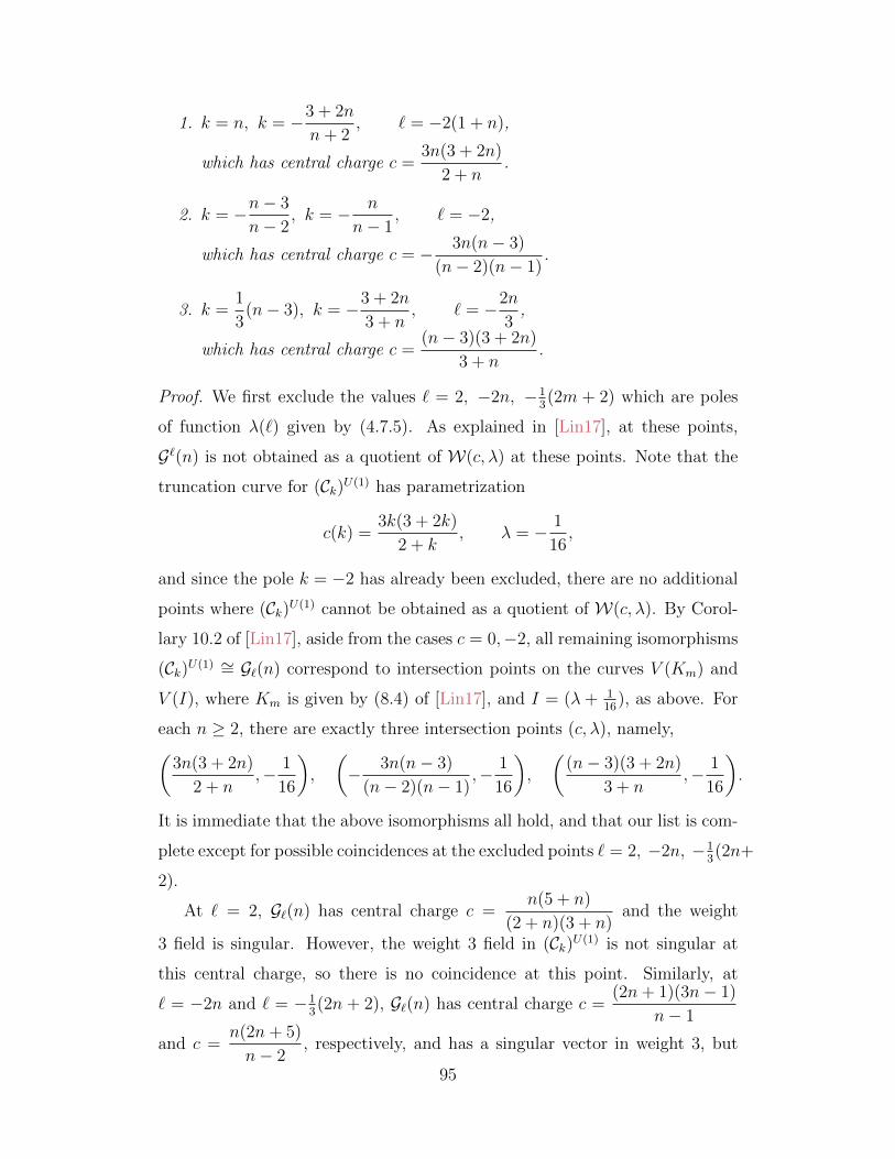
1. k = n, k = −3 + 2n

n+ 2, ` = −2(1 + n),

which has central charge c =3n(3 + 2n)

2 + n.

2. k = −n− 3

n− 2, k = − n

n− 1, ` = −2,

which has central charge c = − 3n(n− 3)

(n− 2)(n− 1).

3. k =1

3(n− 3), k = −3 + 2n

3 + n, ` = −2n

3,

which has central charge c =(n− 3)(3 + 2n)

3 + n.

Proof. We first exclude the values ` = 2, −2n, −13(2m + 2) which are poles

of function λ(`) given by (4.7.5). As explained in [Lin17], at these points,

G`(n) is not obtained as a quotient of W(c, λ) at these points. Note that the

truncation curve for (Ck)U(1) has parametrization

c(k) =3k(3 + 2k)

2 + k, λ = − 1

16,

and since the pole k = −2 has already been excluded, there are no additional

points where (Ck)U(1) cannot be obtained as a quotient of W(c, λ). By Corol-

lary 10.2 of [Lin17], aside from the cases c = 0,−2, all remaining isomorphisms

(Ck)U(1) ∼= G`(n) correspond to intersection points on the curves V (Km) and

V (I), where Km is given by (8.4) of [Lin17], and I = (λ + 116

), as above. For

each n ≥ 2, there are exactly three intersection points (c, λ), namely,(3n(3 + 2n)

2 + n,− 1

16

),

(− 3n(n− 3)

(n− 2)(n− 1),− 1

16

),

((n− 3)(3 + 2n)

3 + n,− 1

16

).

It is immediate that the above isomorphisms all hold, and that our list is com-

plete except for possible coincidences at the excluded points ` = 2, −2n, −13(2n+

2).

At ` = 2, G`(n) has central charge c =n(5 + n)

(2 + n)(3 + n)and the weight

3 field is singular. However, the weight 3 field in (Ck)U(1) is not singular at

this central charge, so there is no coincidence at this point. Similarly, at

` = −2n and ` = −13(2n + 2), G`(n) has central charge c =

(2n+ 1)(3n− 1)

n− 1

and c =n(2n+ 5)

n− 2, respectively, and has a singular vector in weight 3, but

95

at these central charges, (Ck)U(1) does not. Therefore there are no additional

coincidences at these points.

Remark 4.7.7. The first family (1) in Theorem 4.7.6 is of particular in-

terest since it concerns the case where k is a positive integer n. By Re-

mark 4.6.3, the map V n(sl2) → V n(n4) descends to a map of simple ver-

tex algebras Ln(sl2) → Vn(n4). By Corollary 2.2 of [ACKL17], the coset

Com(Ln(sl2), Vn(n4)) is simple, and hence coincides with the simple quotient

Cn of Cn. Moreover, by [DLM96], the simplicity of Cn is preserved by taking

the U(1)-orbifold. It follows that for all n ∈ N,

Com(Ln(sl2), Vn(n4)) ∼= G−2(1+n)(n).

In the case n = 1, note that G−4(1) is just the parafermion algebraN−4(sl2) =

Com(H, L−4(sl2)). Therefore V1(n4) may be regarded as an extension of L1(sl2)⊗

N−4(sl2). Likewise, V1(n4)Z/2Z, which is isomorphic to the global section alge-

bra of the chiral de Rham complex of an Enriques surface, is an extension of

H⊗N−4(sl2), where H is the Heisenberg algebra generated by J .

Consider the coset Com(V k+2(sln)⊗H(1), Lk(sln+1)⊗ E(2n)

)where E(2n)

denotes the bc-system of rank 2n and the Heisenberg algebra action is taken

to be the diagonal one in such a way that this coset has four odd dimension

3/2 fields. Its weight one subspace is H(1) ⊗ Ln(sl2) and if we specialize to

k = −2(n+1) then it is easy to check that the H(1) becomes central and so by

uniqueness of minimal W-superalgebras [ACKL17, Thm. 3.1] at this level the

coset contains Vn(n4) as subalgebra. This fits into the observation of the first

family (1) in Theorem 4.7.6 as this coset also obviously contains G−2(1+n)(n).

This observation somehow extends to negative levels and thus connects

Theorems 4.7.5 and 4.7.6. For this consider the coset

Com(V k−2(sln)⊗H(1), Lk(sln|1)⊗ S(2n)

).

The rank 2n βγ-system S(2n) carries an action of V −n(sl2)⊗V −2(sln)⊗H(1)

and in the commutant we choose the Heisenberg diagonally so that the coset

has four dimension 3/2 fields. As in the previous case the weight one sub-

space is H(1) ⊗ V −n(sl2) and if we specialize to k = −2(n − 1) then it

96

is easy to check that the H(1) becomes central and so by uniqueness of

minimal W-superalgebras [ACKL17, Thm. 3.1] at this level the coset con-

tains a homomorphic image of V −n(n4) as subalgebra. This coset also con-

tains SGk(n) := Com(V k(sln)⊗H(1), Lk(sln|1)

)as subalgebra, and its central

charge for k = −2(n−1) is precisely −3(2n2 − 3n)

n− 2, which is the central charge

of (C−n)U(1) ∼= W`(sl2(n−1), fprin) at ` = −2(n − 1) +n− 2

n− 1. This observation

actually leads us to a new level-rank duality that we will introduce in section

4.8.

Remark 4.7.8. There is another interesting family of vertex algebras that

are expected to arise as quotients of W(c, λ), namely, the cosets

D`(n) = Com(H,W`(sln, fsubreg);

see Conjecture 9.4 of [Lin17]. The explicit truncation curve was given in Con-

jecture 9.6 of [Lin17], and these conjectures were proven in the first nontrivial

case n = 4. Conjecture 9.6 of [Lin17] has the following consequence.

Conjecture 4.7.9. For n ≥ 3, aside from the critical levels k = −2 and

` = −n, and the degenerate cases given by Theorem 10.1 of [Lin17], all iso-

morphisms (Ck)U(1) ∼= D`(n) appear on the following list.

1. k = − n

1 + n, k = −3 + n

2 + n, ` = −n+

2 + n

1 + n, which has central charge

c = − 3n(3 + n)

(1 + n)(2 + n).

2. k = −n, k =3− 2n

−2 + n, ` = −n +

n− 2

n− 1, which has central charge

c = −3n(2n− 3)

n− 2.

3. k = −1

3(3 + n), k =

3− 2n

n− 3, ` = −n +

n

n− 3, which has central

charge c = −(3 + n)(2n− 3)

n− 3.

The proof that this conjecture follows from Conjecture 9.6 of [Lin17] is

similar to the proof of Theorem 4.7.6, and is left to the reader.

97

4.8 Level-rank dualities

We will now explain that the central charge agreement observed in Remark

4.7.7 is not a coincidence and it fits into the following bigger picture. Firstly,

the central charge of the cosets SG−m(n) and of

Com(V −n+1(slm), L−n(slm)⊗ L1(slm)

)(4.8.1)

are both equal to

c = m− 1− m(m2 − 1)

(m− n)(m− n+ 1).

On the other hand recall that the simple quotient of the coset in (4.8.1) is

isomorphic to W`(slm, fprin) at level ` = −m + m−nm−n+1

by the main Theorem

of [ACL19].

We can be more general, namely consider now

SG−m(n|r) := Com(V −m(sln)⊗ V m(slr)⊗H(1), L−m(sln|r)

)together with

Com(V −n+r(slm), L−n(slm)⊗ Lr(slm)

)and again there central charges turn out to coincide, i.e. they are equal to

c =(m2 − 1)nr(n− r − 2m)

(m− n)(m+ r)(m+ r − n).

This observation can be lifted to a new type of level-rank duality. For

this consider E(mn)⊗S(`n) and recall that we denote by E(m) the bc-system

of rank m and by S(m) the βγ-system of rank m. The vertex superalgebra

E(mn) ⊗ S(`n) is viewed as the bcβγ-system for Cn ⊗ Cm|`, i.e. for the ten-

sor product of the standard representations of gln and slm|`. It thus carries

a commuting action of V m−`(gln) ∼= V m−`(sln) ⊗ H(1) and V n(slm|`). We

normalize the Heisenberg field to have norm one, so that the b, c, β and γ all

have Heisenberg weight µ = 1√n(m−`)

. The conformal weight ∆ of the module

V m−`(ω1)⊗ πµ ⊗ V n(ω1) of V m−`(sln)⊗H(1)⊗ V n(slm|`) is

∆ =(n2 − 1)

2(n+m− `)+

1

2n(m− `)+

((m− `)2 − 1)

2(n+m− `)=

1

2

98

so that [AKM+16, Corollary 2.2] applies, i.e. there is a conformal embedding

of V m−`(sln)⊗H(1)⊗ V n(slm|`) in E(mn)⊗ S(`n). We set

An(slm|`) := Com(V m−`(gln), E(mn)⊗ S(`n)

)and if m = 0, then we write A−n(sl`) for An(sl0|`). For descriptions of some of

the cosets of these types see [LSS15]. We also need [OS14, Thm. 4.1], i.e.

Com (Ln(glm), E(mn)) ∼= Lm(sln). (4.8.2)

With this notation and information we can slightly modify the argument of

[ACL19, Thm. 13.1] to get

Com(V −n+r(slm), A−n(slm)⊗ Lr(slm)

) ∼=∼= Com

(V −n+r(slm),Com

(V −m(gln)⊗ Lm(glr),S(mn)⊗ E(mr)

))∼= Com

(V −n+r(slm)⊗ V −m(gln)⊗ Lm(glr),S(mn)⊗ E(mr)

)∼= Com

(V −n+r(glm)⊗ V −m(sln)⊗ Lm(slr)⊗H(1),S(mn)⊗ E(mr)

)∼= Com

(V −m(sln)⊗ Lm(slr)⊗H(1),Com

(V −n+r(glm),S(mn)⊗ E(mr)

))∼= Com

(V −m(sln)⊗ Lm(slr)⊗H(1), Am(slr|n)

)We thus have proven the level-rank duality theorem

Theorem 4.8.1. Let r, n,m be positive integers, then there exist vertex alge-

bra extensions A−n(slm) and Am(slr|n) of homomorphic images V −n(slm) and

V m(slr|n) of V −n(slm) and V m(slr|n) such that the level-rank duality

Com(V −n+r(slm),A−n(slm)⊗ Lr(slm)

)∼=

Com(V −m(sln)⊗ Lm(slr)⊗H(1), Am(slr|n)

)holds.

Remark 4.8.2. It is natural to ask if the statement of the Theorem can be

improved, i.e. one could ask for a level-rank duality of the form

Com(V −n+r(slm),V −n(slm)⊗ Lr(slm)

) ??∼=

Com(V −m(sln)⊗ Lm(slr)⊗H(1), V m(slr|n)

).

99

Remark 4.8.3. One might wonder if there are other levels k for which the

coset Com(V k(sln)⊗ V −k(slr)⊗H(1), V k(sln|r)

)coincides with a W-algebra

and indeed there are indications that these cosets sometimes coincide with

rectangular W-algebras of type A [CH19b, Appendix D].

100

Chapter 5

Lattice VOAs and vertexalgebras of Odake type

Let K be an integral lattice. The associated vertex algebra VK may be ex-

tended by a simple current J(z). Denote the resulting lattice obtained by this

extension by L and let L+ ⊂ L denote its maximal even sublattice. The lat-

tice L is required to be integral in order to have a well-defined vertex algebra

structure. From this it can be seen that the only input data is given by the

tuple (K, δ) where δ has to satisfy certain restrictions in order for L to be

integral. Let K be of rank r and generated by xi such that (xi,xj)K = kδi,j

for k ∈ N. In this chapter we assume that J(z) is a diagonal simple current. In

other words, K is isomorphic to (√kZ)r, the extended lattice L can be defined

by a free resolution

0 −→ Z fδ−→ δZ⊕K −→ L −→ 0,

and the syzygy coming from the image of fδ can be given by

−`δ +r∑i=1

xi = 0.

In order for L to be integral it is required that kr`2, k`∈ Z. The case 1

`∈ Z

is excluded as δ would span only a sublattice and so K ∼= L. The conditions

are equivalent to `|k and `|r, or `2|k. It is immediate that if k is prime then

r = kd for d ∈ N.

In what follows we will restrict to the case k = 3. Recall that the vertex

algebra V√3Z has a N = 2 superconformal structure and is, as is well known,

101

isomorphic to V1(n2). Hence, VL is in particular an extension of V1(n2) ⊂

VK . This will be the reason for the restriction of k. We may express the

generators of K via a Euclidean basis xi =√

3ei and write δ = 1√3(1, . . . , 1).

The important associated lattices are listed below.1 Note that Ds denotes the

lattice of type D of rank s.

L+ =1⋃

n=−1

(2nδ +√

3D3d)

L∗ =

1√3λ ∈ 1√

3Z3d

∣∣ 2 3d∑i=1

λi ≡ 0 mod 3

(5.0.1)

L∗+ =

1√3λ ∈ 1√

3D∗3d

∣∣ 2 3d∑i=1

λi ≡ 0 mod 3

5.1 Embedding VOAs of Odake type

In this section we provide a definition of the Odake vertex algebra Od and

show that it embeds into the lattice vertex superalgebra VL in any dimen-

sion d. Before moving on to the general case we first give a proof of this for

d = 1, 2, 3. This will be proved by constructing a sub vertex algebra of VLthat is isomorphic to Od.

Consider the vertex algebra V = H(2d) ⊗ E(d). Let the sets of strong

generators of the Heisenberg sub vertex algebra and the bc-system be given

by xi(z), yi(z)di=1 and bi(z), ci(z)di=1, respectively. Define a SU(d)-module

structure on V as follows: Let the group action on

(x1(z), . . . , xd(z)) and (b1(z), . . . , bd(z))

be given by the standard representation and the action on

(y1(z), . . . , yd(z)) and (ci(z), . . . , cd(z))

be given by the dual representation. Let Sn be the symmetric group of degree

n.

1Note that the definition of L∗ contains a multiple of 2 which is unnecessary but willmake the decomposition L∗/L more apparent.

102

Proposition 5.1.1. The vertex algebra VSU(d) is strongly generated by the

fields

trm,n(X, Y ) =d∑i=1

: ∂mX i(z)∂nY i(z) : (5.1.1)

for X ∈ x, b and Y ∈ y, c and

detm1,...,md(Z(1), · · · , Z(d)) =∑g∈Sd

g(: ∂m1Z1(1)(z) · · · ∂mdZd

(d)(z) :) (5.1.2)

for Z(1), . . . , Z(d) ∈ x, b and Z(1), . . . , Z(d) ∈ y, c where

: ∂m1Z1(1)(z) · · · ∂mdZd

(d)(z) :

is an element of the non-trivial 1-dimensional Sd-module with the obvious

group action.

Proof. Let V = (W,1, T,Y). Furthermore, let V and V ∗ be the SU(d)-modules

which correspond to the standard and dual representation, respectively. Com-

patibility of W as a SU(d)-module with the vertex algebra structure demands

that the group action is equivariant with respect to the map Y and the trans-

lation operator T . It follows that

(∂nz1(z), . . . , ∂nzd(z)), equivalently (z1−n−1, . . . , z

d−n−1),

is isomorphic to V as a SU(d)-module if z ∈ x, b, and isomorphic to V ∗ as

a SU(d)-module if z ∈ y, c for all n ∈ N0. The space of states W is linearly

isomorphic to

C[x1−1, . . . , x

d−1, x

1−2, . . . , x

d−2, . . . ]⊗ C[y1

−1, . . . , yd−1, y

1−2, . . . , y

d−2, . . . ]⊗

⊗ Λ[b10, . . . , b

d0, b

1−1, . . . , b

d−1, . . . ]⊗ Λ[c1

−1, . . . , cd−1, c

1−2, . . . , c

d−2, . . . ]

Let V = ⊕∞n=1V . It is clear that the space of states W as a SU(d)-module can

now be identified with

S(V)⊗ S(V∗)⊗∧

(V)⊗∧

(V∗)

where V∗ is understood to be the restricted dual, i.e. V∗ = ⊕∞n=1V∗. The

definition of the symmetric and of the antisymmetric algebra makes it obvious

that W is a SU(d)-submodule of

T (V)def= T (V)⊗ T (V)⊗ T (V∗)⊗ T (V∗)

103

where T (C) denotes the usual tensor algebra of a module C. It follows that

W SU(d) ⊂ T (V)SU(d). The SU(d)-invariants of T (V) for V = ⊕ni=1V have

been computed in [Wey46] and are well known to be given by traces and

determinants. Weyl’s proof can be extended to the countably infinite setting

at hand to yield the same invariants.

Definition 5.1.2. The Odake vertex algebra Od ⊂ VSU(d) is the sub vertex

algebra strongly generated by the fields

tr0,0(x, y), tr0,0(x, c), tr0,0(b, y), tr0,0(b, c)

det0,...,0(b, . . . , b), det0,...,0(x, b, . . . , b)

det0,...,0(c, . . . , c), det0,...,0(y, c, . . . , c)

Note that the Odake vertex algebra is by definition a sub vertex algebra

of H(2d) ⊗ E(d) and thus a sub vertex algebra of a (bc − βγ)-system of rank

d. Recall from section 2.2 that over an affine open subset U of a scheme X

of finite type over C the vertex algebra associated to Γ(U,Ωch) is isomorphic

to a (bc − βγ)-system of rank dimC(X). If X is a Calabi-Yau manifold then

the vertex algebra associated to Γ(X,Ωch) contains a N = 2 structure and the

holonomy group is SU(dimC(X)) by definition. Observe that Od is isomorphic

to an extension of V3d(n2) and defined as a sub vertex algebra of the SU(d)-

invariant sub vertex algebra of a (bc − βγ)-system of rank d. We formulate

the following

Conjecture 5.1.3. Let X be a Calabi-Yau d-fold. Then

Od ∼= H0(X,Ωch).

Remark 5.1.4. It is easy to show that O2 is isomorphic to the small N = 4

vertex algebra at central charge 6. The main result of [Son16] is that this

vertex algebra is isomorphic to H0(X,Ωch) for any complex K3 surface X.

Remark 5.1.5. It was shown in [EHKZ13] that O3 is a sub vertex algebra of

H0(X,Ωch) for any Calabi-Yau threefold X.

104

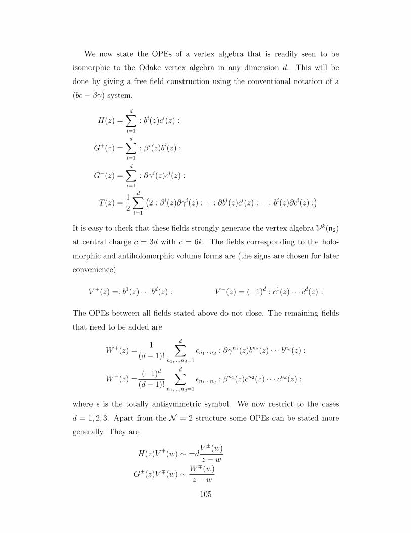
We now state the OPEs of a vertex algebra that is readily seen to be

isomorphic to the Odake vertex algebra in any dimension d. This will be

done by giving a free field construction using the conventional notation of a

(bc− βγ)-system.

H(z) =d∑i=1

: bi(z)ci(z) :

G+(z) =d∑i=1

: βi(z)bi(z) :

G−(z) =d∑i=1

: ∂γi(z)ci(z) :

T (z) =1

2

d∑i=1

(2 : βi(z)∂γi(z) : + : ∂bi(z)ci(z) : − : bi(z)∂ci(z) :

)It is easy to check that these fields strongly generate the vertex algebra Vk(n2)

at central charge c = 3d with c = 6k. The fields corresponding to the holo-

morphic and antiholomorphic volume forms are (the signs are chosen for later

convenience)

V +(z) =: b1(z) · · · bd(z) : V −(z) = (−1)d : c1(z) · · · cd(z) :

The OPEs between all fields stated above do not close. The remaining fields

that need to be added are

W+(z) =1

(d− 1)!

d∑n1,...,nd=1

εn1···nd : ∂γn1(z)bn2(z) · · · bnd(z) :

W−(z) =(−1)d

(d− 1)!

d∑n1,...,nd=1

εn1···nd : βn1(z)cn2(z) · · · cnd(z) :

where ε is the totally antisymmetric symbol. We now restrict to the cases

d = 1, 2, 3. Apart from the N = 2 structure some OPEs can be stated more

generally. They are

H(z)V ±(w) ∼ ±dV±(w)

z − w

G±(z)V ∓(w) ∼ W∓(w)

z − w

105

T (z)V ±(w) ∼ d

2

V ±(w)

(z − w)2+∂V ±(w)

z − w

H(z)W±(w) ∼ ±(d− 1)W±(w)

z − w

G±(z)W±(w) ∼ dV ±(w)

(z − w)2+∂V ±(w)

z − w

T (z)W±(w) ∼ d+ 1

2

W±(w)

(z − w)2+∂W±(w)

z − w

The remaining OPEs are between the fields V +(z), V −(z), W+(z), and W−(z).

The non-regular ones are stated below.

d = 1.

V ±(z)V ∓(w) ∼ − 1

z − w

W±(z)W∓(w) ∼ − 1

(z − w)2

d = 2.

V ±(z)V ∓(w) ∼ − 1

(z − w)2∓ H(z)

z − w

V ±(z)W∓(w) ∼ G±(z)

z − w

W±(z)W∓(w) ∼ 2

(z − w)3∓ H(z)

(z − w)2+T (z)± 1

2∂H(z)

z − w

d = 3.

V ±(z)V ∓(w) ∼ 1

(z − w)3± H(z)

(z − w)2+

1

2

: H(z)H(z) : ±∂H(z)

z − w

V ±(z)W∓(w) ∼ G±(z)

(z − w)2± : H(z)G±(z) :

z − w

W+(z)W−(w) ∼ 3

(z − w)4+

2H(z)

(z − w)3+T (z) + ∂H(z) + 1

2: H(z)H(z) :

(z − w)2

+∂T (z)+ : T (z)H(z) : − : G+(z)G−(z) : +1

2: ∂H(z)H(z) :

z − w

W−(z)W+(w) ∼ 3

(z − w)4− 2H(z)

(z − w)3+T (z)− ∂H(z) + 1

2: H(z)H(z) :

(z − w)2

106

+∂T (z)− : T (z)H(z) : − : G−(z)G+(z) : +1

2: ∂H(z)H(z) :

z − w.

In order to compute the OPEs of the lattice vertex superalgebra explicitly

it is required to choose a non-trivial element ε ∈ H2(L,C×) that satisfies (2.7).

The following Lemma constructs such an element explicitly.

Lemma 5.1.6. An element ε ∈ H2(L,C×) satisfying (2.7) can be chosen to

satisfy the following conditions:

1.

ε(xi,xj) =

−1 if i < j

1 if i ≥ j

2.

ε(xi, δ) = (−1)d+1ε(δ,xi) = (−1)d+i

3.

ε(δ, δ) = (−1)d2

(9d+5) =

−1 if d ≡ 1, 2 mod 4

1 if d ≡ 0, 3 mod 4

Proof. Recall from the construction of L that there exists an injective map

f : K → L and K is freely generated over the set xi. In Remark 5.5a in

[Kac98] a 2-cocycle with values in ±1 which in addition satisfies condition

(2.7) was constructed explicitly. Moreover, this function is bimultiplicative.

We set ε to equal this function under pullback f∗(ε). Part 1 is the result of

this construction.

Part 2 follows from condition (2.5). Note that this also implies the equality

ε(α,−β) = ε(α, β) for α, β ∈ L.

1 = ε(α, 0) = ε(α, 3δ −3d∑i=1

xi) = ε(α, δ)3d∏i=1

ε(α,xi)

Using the same argument on ε(0, α) it now follows from part 1 that ε(xi, δ) =

(−1)i+1. Some thought yields the equality ε(xi, δ) = (−1)d+1ε(δ,xi). This

proves part 2.

The first equality in part 3 is an easy consequence of part 2. The second

equality follows from basic modular arithmetic.

107

Proposition 5.1.7. Let VL be the vertex superalgebra associated to the lattice

L of the previous section. There exists a vertex algebra embedding

ι : Od → VL

in dimensions 1,2 and 3.

Proof. The fields

J(z) =1

3

3d∑i=1

Y (xi−1 ⊗ 1, z) =1

3

3d∑i=1

xi(z) = δ(z)

Q±(z) =1√3

3d∑i=1

Y (1⊗ e±xi , z) =1√3

3d∑i=1

V±xi(z)

L(z) =1

6

3d∑i=1

: Y (xi−1 ⊗ 1, z)Y (xi−1 ⊗ 1, z) :=1

6

3d∑i=1

: xi(z)xi(z) :

are a representation of the universal affine vertex algebra V(n2) at central

charge c = 3d with c = 6k. The simple currents

A±(z) = Y (1⊗ e±δ, z) = V±δ(z) (5.1.3)

are primary fields of conformal weight d2. Using the identity ∂Vα(z) =: α(z)Vα(z) :

for α ∈ L the OPEs with the above fields are

J(z)A±(w) ∼ ±d A±(w)

(z − w)2

Q±(z)A∓(w) ∼ B∓(w)

z − w

L(z)A±(w) ∼ d

2

A±(w)

(z − w)2+∂A±(w)

z − w

A±(z)A∓(w) ∼ ε(δ, δ)

(z − w)d

∑k1+2k2+···=n

n,ki∈N0

(z − w)n(±1)∑i ki

(1!)k1k1!(2!)k2k2! · · ·: J(w)k1(∂J(w))k2 · · · : .

We see that in order for the OPEs to close a new field has to be introduced.

B±(z) =1√3

3d∑i=1

ε(xi, δ)V±(δ−xi)(z)

The OPEs with the strong generators of V(n2) are

J(z)B±(w) ∼ ±(d− 1)B±(w)

(z − w)2

108

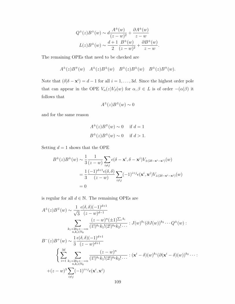
Q±(z)B±(w) ∼ dA±(w)

(z − w)2+∂A±(w)

z − w

L(z)B±(w) ∼ d+ 1

2

B±(w)

(z − w)2+∂B±(w)

z − w.

The remaining OPEs that need to be checked are

A±(z)B∓(w) A±(z)B±(w) B±(z)B±(w) B±(z)B∓(w).

Note that (δ|δ − xi) = d− 1 for all i = 1, . . . , 3d. Since the highest order pole

that can appear in the OPE Vα(z)Vβ(w) for α, β ∈ L is of order −(α|β) it

follows that

A±(z)B±(w) ∼ 0

and for the same reason

A±(z)B∓(w) ∼ 0 if d = 1

B±(z)B±(w) ∼ 0 if d > 1.

Setting d = 1 shows that the OPE

B±(z)B±(w) ∼ 1

3

1

(z − w)

∑i 6=j

ε(δ − xi, δ − xj)V±(2δ−xi−xj)(w)

=1

3

(−1)d+1ε(δ, δ)

(z − w)

∑i 6=j

(−1)i+jε(xi,xj)V±(2δ−xi−xj)(w)

= 0

is regular for all d ∈ N. The remaining OPEs are

A±(z)B∓(w) ∼ 1√3

ε(δ, δ)(−1)d+1

(z − w)d−1∑k1+2k2+···=n

n,ki∈N0

(z − w)n(±1)∑i ki

(1!)k1k1!(2!)k2k2! · · ·: J(w)k1(∂J(w))k2 · · ·Q±(w) :

B−(z)B+(w) ∼ 1

3

ε(δ, δ)(−1)d+1

(z − w)d+13d∑i=1

∑k1+2k2+···=n

n,ki∈N0

(z − w)n

(1!)k1k1!(2!)k2k2! · · ·: (xi − δ)(w)k1(∂(xi − δ)(w))k2 · · · :

+(z − w)3∑i 6=j

(−1)i+jε(xi,xj)

109

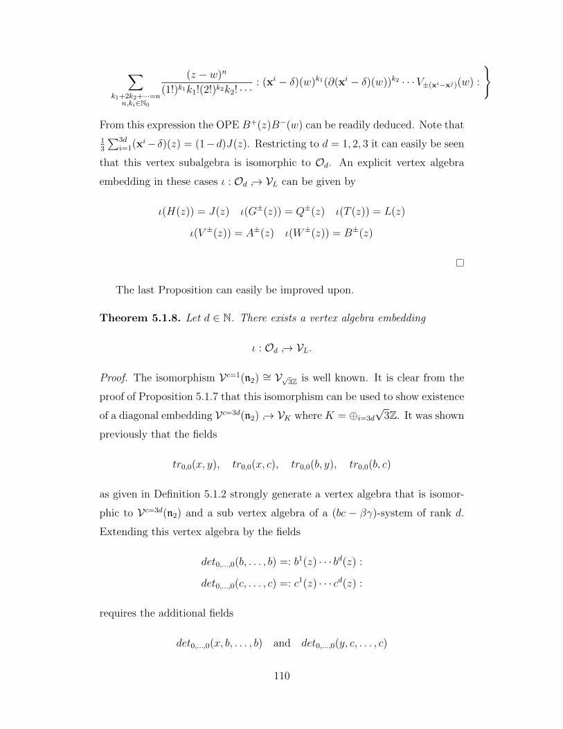
∑k1+2k2+···=n

n,ki∈N0

(z − w)n

(1!)k1k1!(2!)k2k2! · · ·: (xi − δ)(w)k1(∂(xi − δ)(w))k2 · · ·V±(xi−xj)(w) :

From this expression the OPE B+(z)B−(w) can be readily deduced. Note that

13

∑3di=1(xi− δ)(z) = (1−d)J(z). Restricting to d = 1, 2, 3 it can easily be seen

that this vertex subalgebra is isomorphic to Od. An explicit vertex algebra

embedding in these cases ι : Od → VL can be given by

ι(H(z)) = J(z) ι(G±(z)) = Q±(z) ι(T (z)) = L(z)

ι(V ±(z)) = A±(z) ι(W±(z)) = B±(z)

The last Proposition can easily be improved upon.

Theorem 5.1.8. Let d ∈ N. There exists a vertex algebra embedding

ι : Od → VL.

Proof. The isomorphism Vc=1(n2) ∼= V√3Z is well known. It is clear from the

proof of Proposition 5.1.7 that this isomorphism can be used to show existence

of a diagonal embedding Vc=3d(n2) → VK where K = ⊕i=3d

√3Z. It was shown

previously that the fields

tr0,0(x, y), tr0,0(x, c), tr0,0(b, y), tr0,0(b, c)

as given in Definition 5.1.2 strongly generate a vertex algebra that is isomor-

phic to Vc=3d(n2) and a sub vertex algebra of a (bc − βγ)-system of rank d.

Extending this vertex algebra by the fields

det0,...,0(b, . . . , b) =: b1(z) · · · bd(z) :

det0,...,0(c, . . . , c) =: c1(z) · · · cd(z) :

requires the additional fields

det0,...,0(x, b, . . . , b) and det0,...,0(y, c, . . . , c)

110

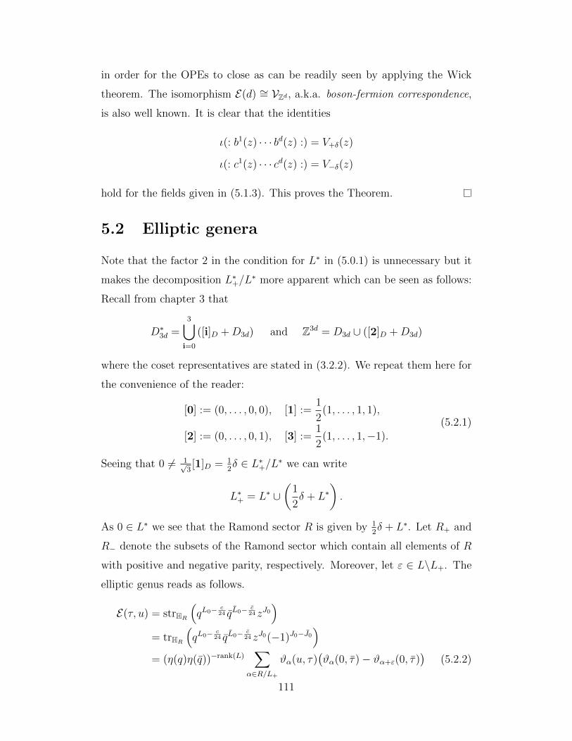
in order for the OPEs to close as can be readily seen by applying the Wick

theorem. The isomorphism E(d) ∼= VZd , a.k.a. boson-fermion correspondence,

is also well known. It is clear that the identities

ι(: b1(z) · · · bd(z) :) = V+δ(z)

ι(: c1(z) · · · cd(z) :) = V−δ(z)

hold for the fields given in (5.1.3). This proves the Theorem.

5.2 Elliptic genera

Note that the factor 2 in the condition for L∗ in (5.0.1) is unnecessary but it

makes the decomposition L∗+/L∗ more apparent which can be seen as follows:

Recall from chapter 3 that

D∗3d =3⋃

i=0

([i]D +D3d) and Z3d = D3d ∪ ([2]D +D3d)

where the coset representatives are stated in (3.2.2). We repeat them here for

the convenience of the reader:

[0] := (0, . . . , 0, 0), [1] :=1

2(1, . . . , 1, 1),

[2] := (0, . . . , 0, 1), [3] :=1

2(1, . . . , 1,−1).

(5.2.1)

Seeing that 0 6= 1√3[1]D = 1

2δ ∈ L∗+/L∗ we can write

L∗+ = L∗ ∪(

1

2δ + L∗

).

As 0 ∈ L∗ we see that the Ramond sector R is given by 12δ + L∗. Let R+ and

R− denote the subsets of the Ramond sector which contain all elements of R

with positive and negative parity, respectively. Moreover, let ε ∈ L\L+. The

elliptic genus reads as follows.

E(τ, u) = strHR

(qL0− c

24 qL0− c24 zJ0

)= trHR

(qL0− c

24 qL0− c24 zJ0(−1)J0−J0

)= (η(q)η(q))−rank(L)

∑α∈R/L+

ϑα(u, τ)(ϑα(0, τ)− ϑα+ε(0, τ)

)(5.2.2)

111

As usual, q = exp(2πiτ) and z = exp(2πiu) where τ, u ∈ C such that =(τ) >

0. The elliptic genus is known to be independent of q, hence we look at

all terms in the sums which cancel the contributions coming from η(q)−3d =

q−d8

∏j(1− qj)3d. Here we used that c = rank(N) = 3d. The bilinear form on

the Ramond sector is positive definite and so all exponents of q in any theta

function above are non-negative. Thus, the only terms to determine in the

theta functions ϑβ(0, τ) =∑

γ∈L+q

12

(β+γ)2are the constant terms and those

which cancel the negative exponents in the aforementioned prefactor. Thus,

we look for elements in the Ramond sector µ = 12δ + γ ∈ 1

2δ + L∗ = R such

thatd

8− n =

1

2µ2 ⇐⇒ δγ + γ2 = −2n (5.2.3)

for n ∈ N0. Setting γ = 1√3τ ∈ L∗ ⊂ 1√

3Z3d yields the condition

3d∑i=1

τi(1 + τi) = −6n

It is easy to see that there exist no solutions to this Diophantine equation for

n > 0 and so the only solutions are τi ∈ 0,−1 for all i = 1, . . . , 3d. The

number of solutions equals 23d, however, since γ ∈ L∗ the number reduces to∑dk=0

(3d3k

). We henceforth denote the set of solutions of eq. (5.2.3) containing

exactly 3k entries equal to −1 (up to an overall factor of 1√3) by [k] and the

associated class of modules by [k] = [k]0 ⊕ [k]1. The parity of any element in

[k] is given by k mod 2.

Before we proceed let us make two observations. Note that δ2 = d which

shows that

δ ∈

L+ if 2|dL+ + ε otherwise.

(5.2.4)

It is apparent from this that the parity is given by the dimension d. Note that

the set [d] contains exactly one element. We will abuse notation and denote

this element by the same symbol. Observe that

[d]d mod 2 31

2δ + [d]

L+∼

12δ if 2|d

12δ + ε otherwise

112

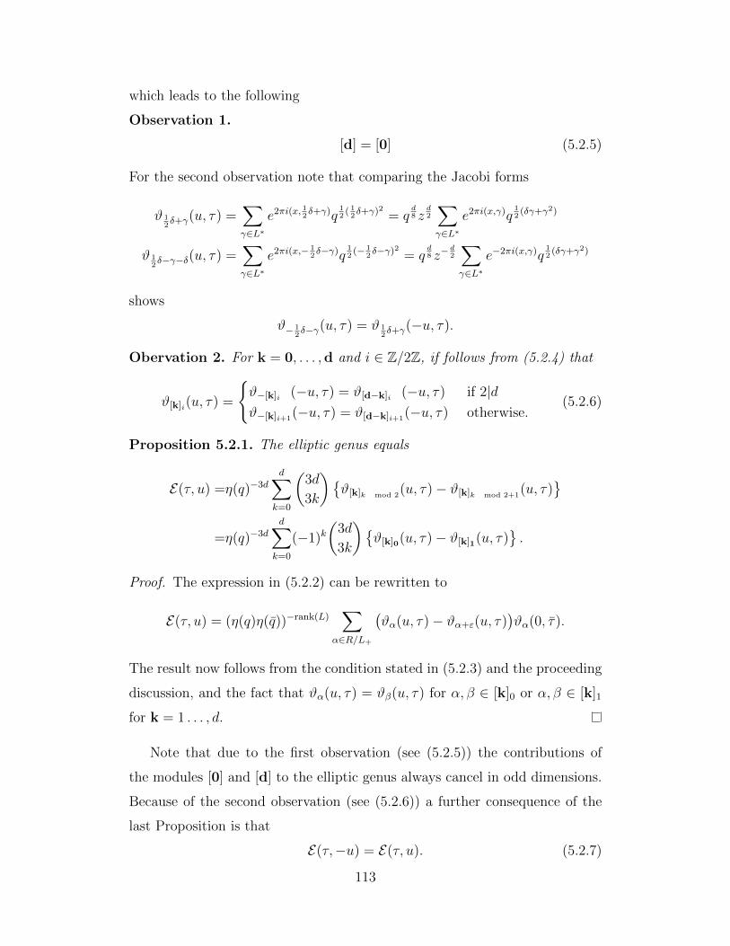
which leads to the following

Observation 1.

[d] = [0] (5.2.5)

For the second observation note that comparing the Jacobi forms

ϑ 12δ+γ(u, τ) =

∑γ∈L∗

e2πi(x, 12δ+γ)q

12

( 12δ+γ)2

= qd8 z

d2

∑γ∈L∗

e2πi(x,γ)q12

(δγ+γ2)

ϑ 12δ−γ−δ(u, τ) =

∑γ∈L∗

e2πi(x,− 12δ−γ)q

12

(− 12δ−γ)2

= qd8 z−

d2

∑γ∈L∗

e−2πi(x,γ)q12

(δγ+γ2)

shows

ϑ− 12δ−γ(u, τ) = ϑ 1

2δ+γ(−u, τ).

Obervation 2. For k = 0, . . . ,d and i ∈ Z/2Z, if follows from (5.2.4) that

ϑ[k]i(u, τ) =

ϑ−[k]i (−u, τ) = ϑ[d−k]i (−u, τ) if 2|dϑ−[k]i+1

(−u, τ) = ϑ[d−k]i+1(−u, τ) otherwise.

(5.2.6)

Proposition 5.2.1. The elliptic genus equals

E(τ, u) =η(q)−3d

d∑k=0

(3d

3k

)ϑ[k]k mod 2

(u, τ)− ϑ[k]k mod 2+1(u, τ)

=η(q)−3d

d∑k=0

(−1)k(

3d

3k

)ϑ[k]0(u, τ)− ϑ[k]1(u, τ)

.

Proof. The expression in (5.2.2) can be rewritten to

E(τ, u) = (η(q)η(q))−rank(L)∑

α∈R/L+

(ϑα(u, τ)− ϑα+ε(u, τ)

)ϑα(0, τ).

The result now follows from the condition stated in (5.2.3) and the proceeding

discussion, and the fact that ϑα(u, τ) = ϑβ(u, τ) for α, β ∈ [k]0 or α, β ∈ [k]1

for k = 1 . . . , d.

Note that due to the first observation (see (5.2.5)) the contributions of

the modules [0] and [d] to the elliptic genus always cancel in odd dimensions.

Because of the second observation (see (5.2.6)) a further consequence of the

last Proposition is that

E(τ,−u) = E(τ, u). (5.2.7)

113

Remark 5.2.2. On a compact complex manifold of dimension d with vanish-

ing first Chern class the elliptic genus is a Jacobi form of weight 0 and index

d2

(see Prop. 1.2 in [Gri00]). A consequence of this is that the elliptic genus

is invariant under the Z/2Z-action induced by −id ∈ SL2(Z) which yields the

relation E(τ,−u) = E(τ, u). Hence, in order for the vertex algebra VL to be

defined on a compact manifold with vanishing first Chern class (5.2.7) is a

necessary condition.

Example 5.2.3. Let d = 1. Recall our first observation which implies [0]k =

[1]k for k ∈ Z/2Z. It follows that the elliptic genus vanishes

E(τ, u) = η(q)−3ϑ[0]0(u, τ)− ϑ[0]1(u, τ) + ϑ[0]1(u, τ)− ϑ[0]0(u, τ) = 0.

The following Jacobi functions are provided for later reference.

ϑ[0]0(u, τ) = ϑ 12δ(u, τ) = q

18 z+ 1

2

(1 + q(6 + z−2) +O(q2)

)ϑ[0]1(u, τ) = ϑ 1

2δ+ε(u, τ) = q

18 z−

12

(1 + q(z2 + 6) +O(q2)

)Example 5.2.4. Let d = 2 and γk ∈ [k]. Since the elliptic genus is a weak

Jacobi form of weight 0 it is uniquely determined by its q0-term if its index is

less than 6 or equal to 132

(see Corollary 1.7 in [Gri00]). The relevant Jacobi

forms are

ϑ[0]0(u, τ) = ϑ 12δ(u, τ) = q

14

(z + z−1 +O(q2)

)ϑ[0]1(u, τ) = ϑ 1

2δ+ε(u, τ) = q

14

(0 + 12q +O(q2)

)ϑ[1]1(u, τ) = ϑ 1

2δ+γ1

(u, τ) = q14

(1 + q(z2 + 6 + z−2) +O(q2)

)ϑ[1]0(u, τ) = ϑ 1

2δ+γ1+ε(u, τ) = q

14

(0 + 7q(z + z−1) +O(q2)

)All of the above theta functions satisfy ϑ[i]k(u, τ) = ϑ[i]k(−u, τ) which is a

consequence of the first and second observation. The elliptic genus equals

E(τ, u) =η(q)−62(ϑ[0]0 − ϑ[0]1) + 20(ϑ[1]1 − ϑ[1]0)

=2(z + 10 + z−1 + q(10z2 − 64z + 108− 64z−1 + 10z−2) +O(q2)

)=2φ0,1.

114

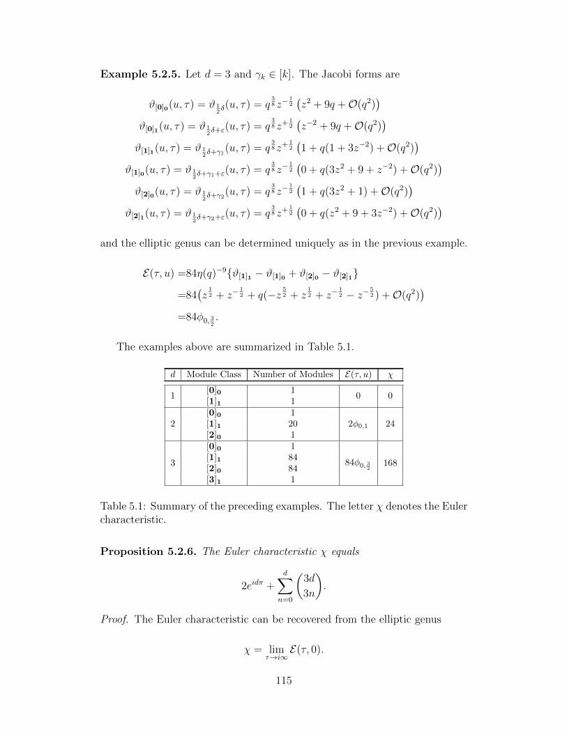
Example 5.2.5. Let d = 3 and γk ∈ [k]. The Jacobi forms are

ϑ[0]0(u, τ) = ϑ 12δ(u, τ) = q

38 z−

12

(z2 + 9q +O(q2)

)ϑ[0]1(u, τ) = ϑ 1

2δ+ε(u, τ) = q

38 z+ 1

2

(z−2 + 9q +O(q2)

)ϑ[1]1(u, τ) = ϑ 1

2δ+γ1

(u, τ) = q38 z+ 1

2

(1 + q(1 + 3z−2) +O(q2)

)ϑ[1]0(u, τ) = ϑ 1

2δ+γ1+ε(u, τ) = q

38 z−

12

(0 + q(3z2 + 9 + z−2) +O(q2)

)ϑ[2]0(u, τ) = ϑ 1

2δ+γ2

(u, τ) = q38 z−

12

(1 + q(3z2 + 1) +O(q2)

)ϑ[2]1(u, τ) = ϑ 1

2δ+γ2+ε(u, τ) = q

38 z+ 1

2

(0 + q(z2 + 9 + 3z−2) +O(q2)

)and the elliptic genus can be determined uniquely as in the previous example.

E(τ, u) =84η(q)−9ϑ[1]1 − ϑ[1]0 + ϑ[2]0 − ϑ[2]1

=84(z

12 + z−

12 + q(−z

52 + z

12 + z−

12 − z−

52 ) +O(q2)

)=84φ0, 3

2.

The examples above are summarized in Table 5.1.

d Module Class Number of Modules E(τ, u) χ

1[0]0 1

0 0[1]1 1[0]0 1

2 [1]1 20 2φ0,1 24[2]0 1[0]0 1

3[1]1 84

84φ0, 32 168[2]0 84[3]1 1

Table 5.1: Summary of the preceding examples. The letter χ denotes the Eulercharacteristic.

Proposition 5.2.6. The Euler characteristic χ equals

2eidπ +d∑

n=0

(3d

3n

).

Proof. The Euler characteristic can be recovered from the elliptic genus

χ = limτ→i∞

E(τ, 0).

115

In order to determine the Euler characteristic we proceed by determining all

terms proportional to q0 in the elliptic genus. Just as in the case of q0 which was

discussed previously this leads to condition (5.2.3). We rewrite this condition

as follows

1

2

(1

2δ + γ + λ

)2

=d

8− n ⇐⇒ γ2 + λ2 + δγ + 2λ

(γ +

1

2δ

)= −2n

where γ ∈ L∗/L+ and λ ∈ L+ and n ∈ N0. As determined previously, this

condition has solutions if and only if n = 0. It follows that γ ∈ [k] and

so no module in a class [k]k mod 2+1 contributes to the Euler characteristic.

Additionally, since γ ∈ [k] we have γ2 +δγ = 0 and the last equation simplifies

to

λ(λ+ δ + 2γ) = 0.

1. λ = 0. The coefficients of the terms proportional to qd8 of the Jacobi

forms ϑ[k]k mod 2are e2πi(x, 1

2δ+γ) = e2πi

√3x( d

2+m) = z

d2

+m where m = −k if

γ ∈ [k].

2. λ+ δ + 2γ = 0. Hence, δ + 2γ ∈ L+. Recall from (5.2.4) that δ ∈ L+ in

even dimensions. It follows that γ can only equal either [0] or [d]. The

same conclusion follows in odd dimensions. The coefficients of the terms

proportional to qd8 of the Jacobi forms ϑ[k]k mod 2

are e2πi(x, 12δ+γ−δ−2γ) =

e−2πi√

3x( d2

+m) = z−( d2

+m) where γ ∈ [0] and m = 0 or γ ∈ [d] and

m = −d. Thus, for even d, the condition δ + 2γ ∈ L+ suggests that

only the module [0]0 = [d]0 yields non zero terms to the elliptic genus.

For odd d the module [0]1 = [d]1 could contribute as well, however,

contributions from the vacuum module always cancel if d is odd due to

Observation 1 and Proposition 5.2.1.

In summary, every module in a class [k]k mod 2 for k = 1, . . . , d − 1 adds a

factor of 1 to the Euler characteristic and in odd dimensions these are the

only contributions. In even dimensions the only remaining contributions are

from the modules [0]0 and [d]0 where each of which contributes a factor of

2.

116

Corollary 5.2.7. The elliptic genus associated to VL vanishes if and only if

d = 1.

Lemma 5.2.8. The Euler characteristic χ is divisible by 24.

Proof. Using the equality

d∑k=0

(3d

3k

)=

1

3

(23d + 2eidπ

)the Euler characteristic equals

χ =

23

3

(8d−1 + 1

)for even d

23

3

(8d−1 − 1

)for odd d.

By induction, 8even≥0 = 1 mod 32. It follows easily that 8odd>0 = −1 mod 32.

Thus, 24|χ.

d χ

1 02 243 1684 13685 109206 873847 6990488 55924089 4473924010 357913944...

...

Table 5.2: Euler Characteristic for the lowest dimensions.

The definition of the elliptic genus may be extended by inserting a further

Jacobi variable. Following [KT17, Wen19] let HR = φ ∈ HR|(L0 − c24

)φ = 0

and define the Hodge-elliptic genus (cf. Def. 2.2 in [Wen19])

EHodge(τ, u, v) = trHR

(qL0− c

24 zJ0yJ0(−1)J0−J0

).

For an element of an anti-chiral module γ ∈ [k] we have J0(γ) = −√

3k. Thus,

the elliptic genus as given in Prop. 5.2.1 is refined to

EHodge(τ, u, v) =η(q)−3d

d∑k=0

yd2−k(

3d

3k

)ϑ[k]k mod 2

(u, τ)− ϑ[k]k mod 2+1(u, τ)

117

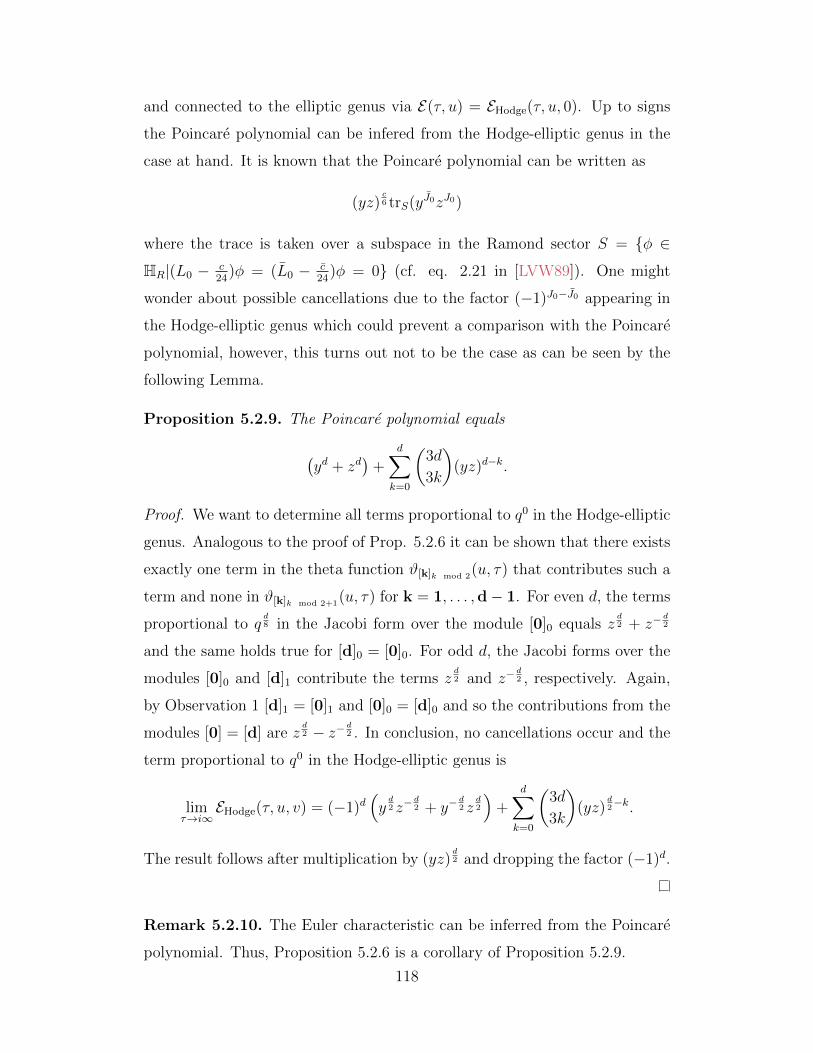
and connected to the elliptic genus via E(τ, u) = EHodge(τ, u, 0). Up to signs

the Poincare polynomial can be infered from the Hodge-elliptic genus in the

case at hand. It is known that the Poincare polynomial can be written as

(yz)c6 trS(yJ0zJ0)

where the trace is taken over a subspace in the Ramond sector S = φ ∈

HR|(L0 − c24

)φ = (L0 − c24

)φ = 0 (cf. eq. 2.21 in [LVW89]). One might

wonder about possible cancellations due to the factor (−1)J0−J0 appearing in

the Hodge-elliptic genus which could prevent a comparison with the Poincare

polynomial, however, this turns out not to be the case as can be seen by the

following Lemma.

Proposition 5.2.9. The Poincare polynomial equals

(yd + zd

)+

d∑k=0

(3d

3k

)(yz)d−k.

Proof. We want to determine all terms proportional to q0 in the Hodge-elliptic

genus. Analogous to the proof of Prop. 5.2.6 it can be shown that there exists

exactly one term in the theta function ϑ[k]k mod 2(u, τ) that contributes such a

term and none in ϑ[k]k mod 2+1(u, τ) for k = 1, . . . ,d− 1. For even d, the terms

proportional to qd8 in the Jacobi form over the module [0]0 equals z

d2 + z−

d2

and the same holds true for [d]0 = [0]0. For odd d, the Jacobi forms over the

modules [0]0 and [d]1 contribute the terms zd2 and z−

d2 , respectively. Again,

by Observation 1 [d]1 = [0]1 and [0]0 = [d]0 and so the contributions from the

modules [0] = [d] are zd2 − z− d2 . In conclusion, no cancellations occur and the

term proportional to q0 in the Hodge-elliptic genus is

limτ→i∞

EHodge(τ, u, v) = (−1)d(yd2 z−

d2 + y−

d2 z

d2

)+

d∑k=0

(3d

3k

)(yz)

d2−k.

The result follows after multiplication by (yz)d2 and dropping the factor (−1)d.

Remark 5.2.10. The Euler characteristic can be inferred from the Poincare

polynomial. Thus, Proposition 5.2.6 is a corollary of Proposition 5.2.9.

118

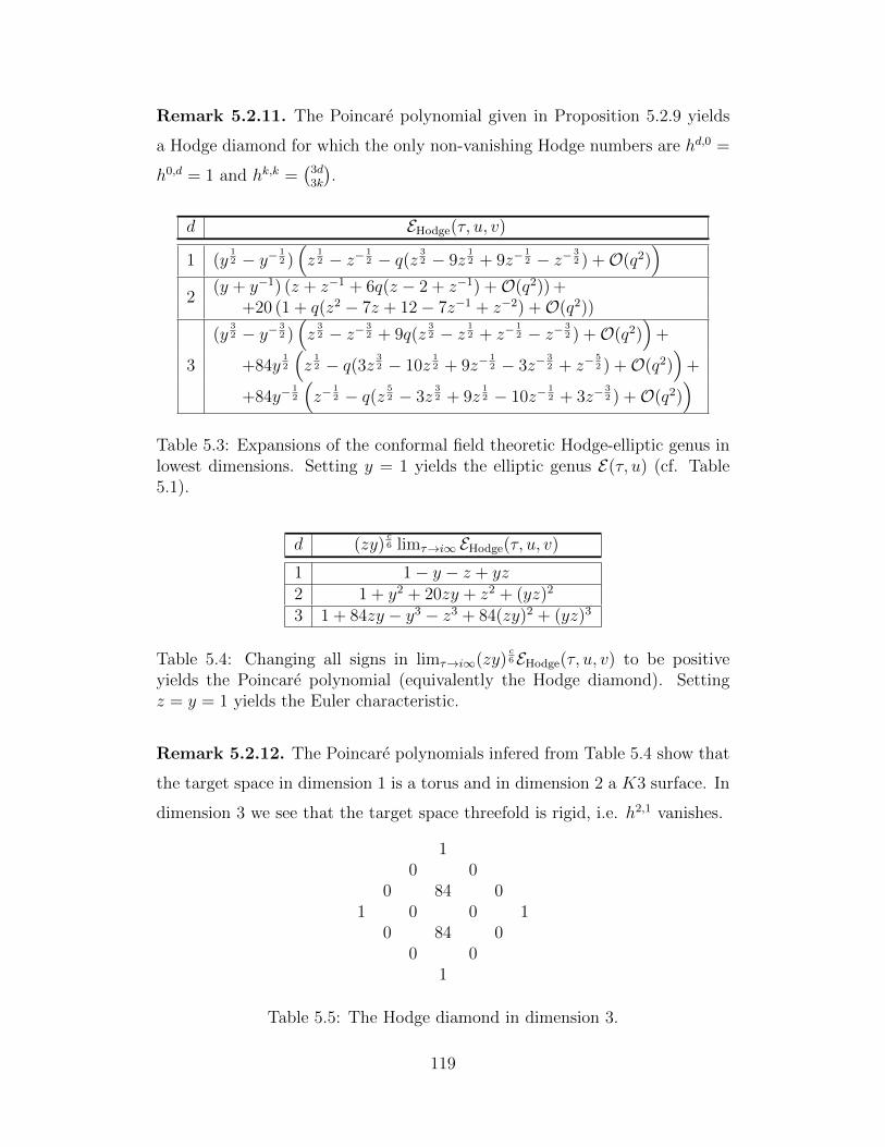
Remark 5.2.11. The Poincare polynomial given in Proposition 5.2.9 yields

a Hodge diamond for which the only non-vanishing Hodge numbers are hd,0 =

h0,d = 1 and hk,k =(

3d3k

).

d EHodge(τ, u, v)

1 (y12 − y− 1

2 )(z

12 − z− 1

2 − q(z 32 − 9z

12 + 9z−

12 − z− 3

2 ) +O(q2))

2(y + y−1) (z + z−1 + 6q(z − 2 + z−1) +O(q2)) +

+20 (1 + q(z2 − 7z + 12− 7z−1 + z−2) +O(q2))

(y32 − y− 3

2 )(z

32 − z− 3

2 + 9q(z32 − z 1

2 + z−12 − z− 3

2 ) +O(q2))

+

3 +84y12

(z

12 − q(3z 3

2 − 10z12 + 9z−

12 − 3z−

32 + z−

52 ) +O(q2)

)+

+84y−12

(z−

12 − q(z 5

2 − 3z32 + 9z

12 − 10z−

12 + 3z−

32 ) +O(q2)

)Table 5.3: Expansions of the conformal field theoretic Hodge-elliptic genus inlowest dimensions. Setting y = 1 yields the elliptic genus E(τ, u) (cf. Table5.1).

d (zy)c6 limτ→i∞ EHodge(τ, u, v)

1 1− y − z + yz2 1 + y2 + 20zy + z2 + (yz)2

3 1 + 84zy − y3 − z3 + 84(zy)2 + (yz)3

Table 5.4: Changing all signs in limτ→i∞(zy)c6EHodge(τ, u, v) to be positive

yields the Poincare polynomial (equivalently the Hodge diamond). Settingz = y = 1 yields the Euler characteristic.

Remark 5.2.12. The Poincare polynomials infered from Table 5.4 show that

the target space in dimension 1 is a torus and in dimension 2 a K3 surface. In

dimension 3 we see that the target space threefold is rigid, i.e. h2,1 vanishes.

10 0

0 84 01 0 0 1

0 84 00 0

1

Table 5.5: The Hodge diamond in dimension 3.

119

Chapter 6

On conformal embeddings ofaffine VOAs into rectangularW-algebras

Let g′ be a Lie algebra such that g′ ⊂ g. Take the sequence of embeddings

sl2 → g′ι→ g

with the first map being the principal embedding. Denote the image of the

sl2-triple by x, e, f where [x, f ] = −f . It is clear that gg′ ⊂ gι(f). Hence, for

any Lie algebra s ⊂ gg′

it follows from the introduction above that

V`(s) →Wk(g, ι(f)).

One may wonder which condition(s) allow(s) for a stronger statement, e.g.

when this embedding is conformal or an isomorphism. A similar question has

been asked in [AKM+18b] where all levels k where found for which the em-

bedding of the maximal affine vertex algebra in a simple minimal W-algebra

Wk(g, θ) is conformal, with g being a simple Lie super-algebra and −θ its min-

imal root. This investigation was continued in [AKM+17] where the decom-

position of the minimal simple affine W-algebra as a module over its maximal

affine vertex algebra was discussed. It is worth mentioning that the authors

showed in a closely related work [AKM+18a] that in case the conformal em-

bedding is an isomorphism, the representation category of the affine VOA is

semi-simple even at non-admissible levels.

120

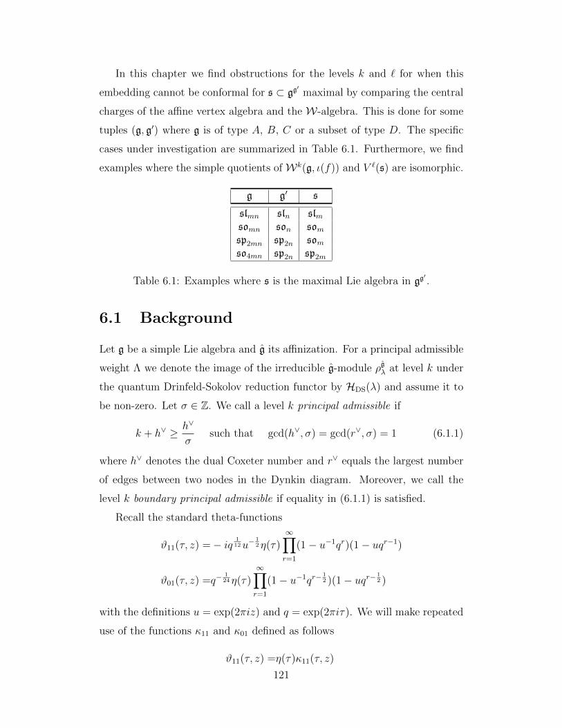
In this chapter we find obstructions for the levels k and ` for when this

embedding cannot be conformal for s ⊂ gg′

maximal by comparing the central

charges of the affine vertex algebra and the W-algebra. This is done for some

tuples (g, g′) where g is of type A, B, C or a subset of type D. The specific

cases under investigation are summarized in Table 6.1. Furthermore, we find

examples where the simple quotients ofWk(g, ι(f)) and V `(s) are isomorphic.

g g′ s

slmn sln slmsomn son somsp2mn sp2n somso4mn sp2n sp2m

Table 6.1: Examples where s is the maximal Lie algebra in gg′.

6.1 Background

Let g be a simple Lie algebra and g its affinization. For a principal admissible

weight Λ we denote the image of the irreducible g-module ρgλ at level k under

the quantum Drinfeld-Sokolov reduction functor by HDS(λ) and assume it to

be non-zero. Let σ ∈ Z. We call a level k principal admissible if

k + h∨ ≥ h∨

σsuch that gcd(h∨, σ) = gcd(r∨, σ) = 1 (6.1.1)

where h∨ denotes the dual Coxeter number and r∨ equals the largest number

of edges between two nodes in the Dynkin diagram. Moreover, we call the

level k boundary principal admissible if equality in (6.1.1) is satisfied.

Recall the standard theta-functions

ϑ11(τ, z) =− iq112u−

12η(τ)

∞∏r=1

(1− u−1qr)(1− uqr−1)

ϑ01(τ, z) =q−124η(τ)

∞∏r=1

(1− u−1qr−12 )(1− uqr−

12 )

with the definitions u = exp(2πiz) and q = exp(2πiτ). We will make repeated

use of the functions κ11 and κ01 defined as follows

ϑ11(τ, z) =η(τ)κ11(τ, z)

121

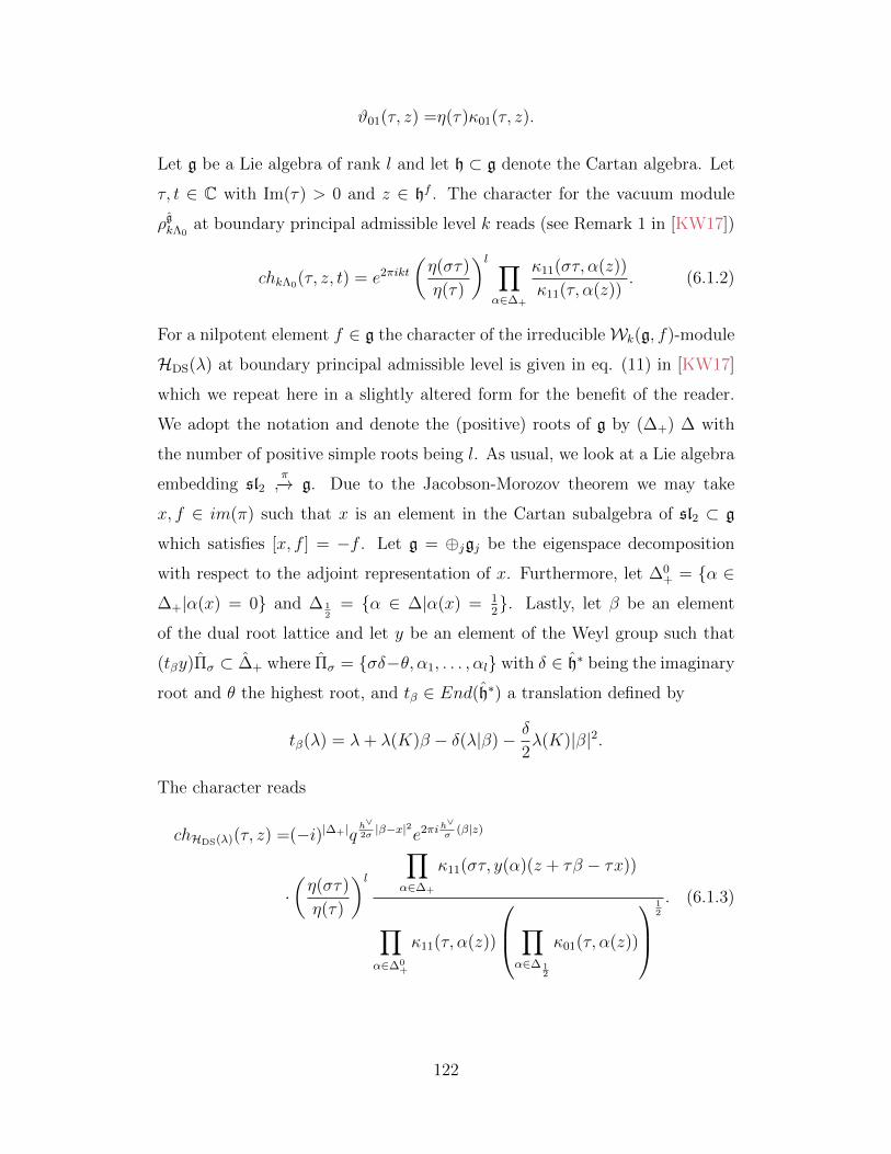
ϑ01(τ, z) =η(τ)κ01(τ, z).

Let g be a Lie algebra of rank l and let h ⊂ g denote the Cartan algebra. Let

τ, t ∈ C with Im(τ) > 0 and z ∈ hf . The character for the vacuum module

ρgkΛ0at boundary principal admissible level k reads (see Remark 1 in [KW17])

chkΛ0(τ, z, t) = e2πikt

(η(στ)

η(τ)

)l ∏α∈∆+

κ11(στ, α(z))

κ11(τ, α(z)). (6.1.2)

For a nilpotent element f ∈ g the character of the irreducibleWk(g, f)-module

HDS(λ) at boundary principal admissible level is given in eq. (11) in [KW17]

which we repeat here in a slightly altered form for the benefit of the reader.

We adopt the notation and denote the (positive) roots of g by (∆+) ∆ with

the number of positive simple roots being l. As usual, we look at a Lie algebra

embedding sl2π−→ g. Due to the Jacobson-Morozov theorem we may take

x, f ∈ im(π) such that x is an element in the Cartan subalgebra of sl2 ⊂ g

which satisfies [x, f ] = −f . Let g = ⊕jgj be the eigenspace decomposition

with respect to the adjoint representation of x. Furthermore, let ∆0+ = α ∈

∆+|α(x) = 0 and ∆ 12

= α ∈ ∆|α(x) = 12. Lastly, let β be an element

of the dual root lattice and let y be an element of the Weyl group such that

(tβy)Πσ ⊂ ∆+ where Πσ = σδ−θ, α1, . . . , αl with δ ∈ h∗ being the imaginary

root and θ the highest root, and tβ ∈ End(h∗) a translation defined by

tβ(λ) = λ+ λ(K)β − δ(λ|β)− δ

2λ(K)|β|2.

The character reads

chHDS(λ)(τ, z) =(−i)|∆+|qh∨2σ|β−x|2e2πih

∨σ

(β|z)

·(η(στ)

η(τ)

)l ∏α∈∆+

κ11(στ, y(α)(z + τβ − τx))

∏α∈∆0

+

κ11(τ, α(z))

∏α∈∆ 1

2

κ01(τ, α(z))

12

. (6.1.3)

122

6.2 Obstructions to conformal embeddings of

maximal affine sub vertex algebras

We adopt the convention that 1 < N ∈ N, take n to be a divisor of N ,

and write N = mn throughout this section. Table 6.2 and Theorem 6.2.1

summarize the findings of this section.

g g′ ⊗ s g type g′ type k + h∨g `+ h∨s

h∨g +1

nh∨s + 1

slmn sln ⊗ slm A Ah∨gn+1

h∨sn+1

h∨g−1

nh∨s − 1

h∨g +2

n+1h∨s +2n+1

somn son ⊗ som B Bh∨g +1

nh∨s + 1

h∨gn

h∨s

h∨gn

h∨s

son ⊗ sp2m Bh∨g− 1

2

nh∨s − 1

2

h∨g−1

n+1h∨s −1n+1

h∨g2n+1

h∨s2n+1

sp2n ⊗ som Ch∨g− 1

2

2nh∨s + 1

sp2mn C

h∨g−m22n−1

2mn−h∨s2n−1

h∨g +1

2nh∨s − 1

2

so4mn sp2n ⊗ sp2m D Ch∨g

2n+1h∨s

2n+1

h∨g−2m

2n−12mn−h∨s

2n−1

Table 6.2: Levels at which the central charges of the rectangular W-algebraWk(g, ι(f)) and the affine vertex algebra V`(s) coincide. Note that s is themaximal Lie algebra in gg

′. For the rectangular vertex algebraWk(g, ι(f)), sl2

is chosen to be principally embedded into g′.

Theorem 6.2.1. For any tuple of Lie algebras (g, s) at boundary principal

admissible level k as stated in Table 6.2 there exists an isomorphism of vertex

123

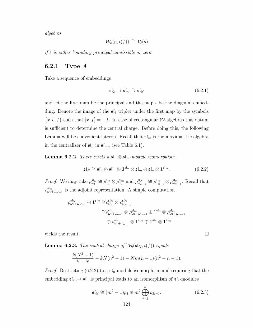
algebras

Wk(g, ι(f))∼−→ V`(s)

if ` is either boundary principal admissible or zero.

6.2.1 Type A

Take a sequence of embeddings

sl2 → slnι→ slN (6.2.1)

and let the first map be the principal and the map ι be the diagonal embed-

ding. Denote the image of the sl2 triplet under the first map by the symbols

x, e, f such that [x, f ] = −f . In case of rectangular W-algebras this datum

is sufficient to determine the central charge. Before doing this, the following

Lemma will be convenient lateron. Recall that slm is the maximal Lie algebra

in the centralizer of sln in slmn (see Table 6.1).

Lemma 6.2.2. There exists a sln ⊗ slm-module isomorphism

slN ∼= sln ⊗ slm ⊕ 1sln ⊗ slm ⊕ sln ⊗ 1slm . (6.2.2)

Proof. We may take ρslNω1∼= ρslnω1

⊗ ρslmω1and ρslNωN−1

∼= ρslnωn−1⊗ ρslmωm−1

. Recall that

ρslNω1+ωN−1is the adjoint representation. A simple computation

ρslNω1+ωN−1⊕ 1slN ∼=ρslNω1

⊗ ρslNωN−1

∼=ρslnω1+ωn−1⊗ ρslmω1+ωm−1

⊕ 1sln ⊗ ρslmω1+ωm−1

⊕ ρslnω1+ωn−1⊗ 1slm ⊕ 1sln ⊗ 1slm

yields the result.

Lemma 6.2.3. The central charge of Wk(slN , ι(f)) equals

k(N2 − 1)

k +N− kN(n2 − 1)−Nm(n− 1)(n2 − n− 1).

Proof. Restricting (6.2.2) to a sln-module isomorphism and requiring that the

embedding sl2 → sln is principal leads to an isomorphism of sl2-modules

slN ∼= (m2 − 1)ρ1 ⊕m2

n⊕j=2

ρ2i−1. (6.2.3)

124

More explicitly, for the second embedding we may take

ι(f) =m−1∑j=0

n−1∑i=1

ejn+i+1,jn+i , ι(x) =1

2

m−1∑j=0

n∑i=1

(n+ 1− 2i)ejn+i,jn+i.

Applying eq. (2.10) then yields the result. The only contributions which

are not straight forward are the ones from the charged and the neutral free

fermions. Using the notation of loc. cit., observe that g 12

= ∅ as can be seen

from (6.2.3) since no sl2-module of even dimension appears in the decompo-

sition. The contribution from the charged free fermions can be infered from

(6.2.3) and equals

−2m2

n−1∑i=1

(n− i)(6i2 − 6i+ 1) = −Nm(n− 1)(n2 − n− 1).

Proposition 6.2.4. All levels k at which the central charges of V `(slm) and

Wk(slN , ι(f)) coincide are

k +N =N

n+ 1and k +N =

N ± 1

n.

Proof. Observe from Lemma 6.2.2 that there are copies of Vk(slm) in the

W-algebra due to the submodule 1sln ⊗ slm ⊂ slN . Furthermore, each set of

ghosts shifts the level by a factor that depends on the representation of slm. All

ghosts that appear are either in the trivial or the adjoint representation of slm.

The former does not contribute to the level shift. This leaves the submodule

sln ⊗ slm ⊂ slN where the number of ghosts needs to be determined, i.e. the

order of the set⊕

i 6=0(sln)i under the induced grading of slN under adx. One

is quick to see that ∣∣∣⊕i 6=0

(sln)i

∣∣∣ = n(n− 1).

The dependence of the levels can now be seen to be

` = kn+mn(n− 1).

The result follows after equating the central charge of V `(slm) with the central

charge of Wk(slN , ι(f)) which is given by Lemma 6.2.3.

125

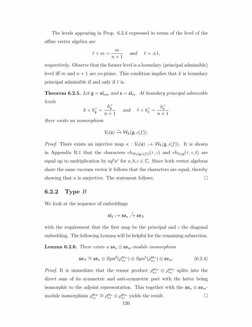
The levels appearing in Prop. 6.2.4 expressed in terms of the level of the

affine vertex algebra are

`+m =m

n+ 1and ` = ±1,

respectively. Observe that the former level is a boundary (principal admissible)

level iff m and n+ 1 are co-prime. This condition implies that k is boundary

principal admissible if and only if ` is.

Theorem 6.2.5. Let g = slmn and s = slm. At boundary principal admissible

levels

k + h∨g =h∨gn+ 1

and `+ h∨s =h∨sn+ 1

there exists an isomorphism

V`(s)∼−→Wk(g, ι(f)).

Proof. There exists an injective map κ : V`(s) → Wk(g, ι(f)). It is shown

in Appendix B.1 that the characters chWk(g,ι(f))(τ, z) and chV`(g(τ, z, t) are

equal up to multiplication by aqbuc for a, b, c ∈ C. Since both vertex algebras

share the same vacuum vector it follows that the characters are equal, thereby

showing that κ is surjective. The statement follows.

6.2.2 Type B

We look at the sequence of embeddings

sl2 → sonι→ soN

with the requirement that the first map be the principal and ι the diagonal

embedding. The following Lemma will be helpful for the remaining subsection.

Lemma 6.2.6. There exists a son ⊗ som-module isomorphism

soN ∼= son ⊗ Sym2(ρsomω1)⊕ Sym2(ρsonω1

)⊗ som. (6.2.4)

Proof. It is immediate that the tensor product ρsoNω1⊗ ρsoNω1

splits into the

direct sum of its symmetric and anti-symmetric part with the latter being

isomorphic to the adjoint representation. This together with the son ⊗ som-

module isomorphism ρsoNω1∼= ρsonω1

⊗ ρsomω1yields the result.

126

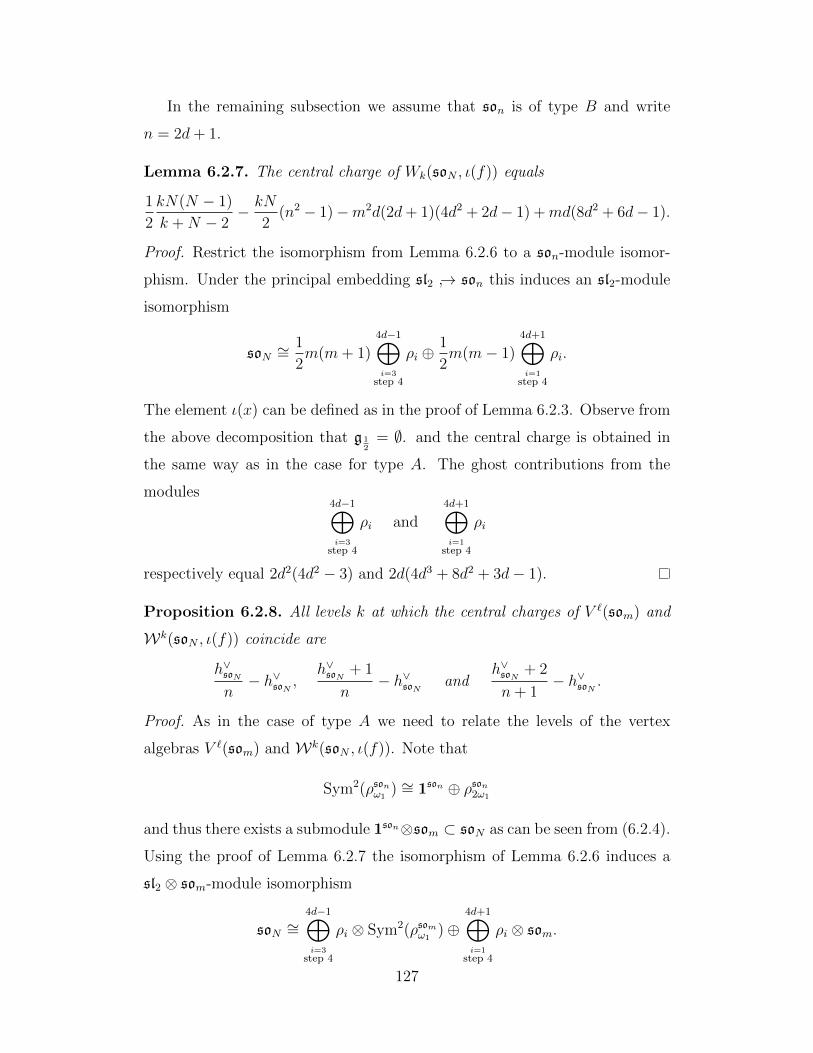
In the remaining subsection we assume that son is of type B and write

n = 2d+ 1.

Lemma 6.2.7. The central charge of Wk(soN , ι(f)) equals

1

2

kN(N − 1)

k +N − 2− kN

2(n2 − 1)−m2d(2d+ 1)(4d2 + 2d− 1) +md(8d2 + 6d− 1).

Proof. Restrict the isomorphism from Lemma 6.2.6 to a son-module isomor-

phism. Under the principal embedding sl2 → son this induces an sl2-module

isomorphism

soN ∼=1

2m(m+ 1)

4d−1⊕i=3

step 4

ρi ⊕1

2m(m− 1)

4d+1⊕i=1

step 4

ρi.

The element ι(x) can be defined as in the proof of Lemma 6.2.3. Observe from

the above decomposition that g 12

= ∅. and the central charge is obtained in

the same way as in the case for type A. The ghost contributions from the

modules4d−1⊕i=3

step 4

ρi and4d+1⊕i=1

step 4

ρi

respectively equal 2d2(4d2 − 3) and 2d(4d3 + 8d2 + 3d− 1).

Proposition 6.2.8. All levels k at which the central charges of V `(som) and

Wk(soN , ι(f)) coincide are

h∨soNn− h∨soN ,

h∨soN + 1

n− h∨soN and

h∨soN + 2

n+ 1− h∨soN .

Proof. As in the case of type A we need to relate the levels of the vertex

algebras V `(som) and Wk(soN , ι(f)). Note that

Sym2(ρsonω1) ∼= 1son ⊕ ρson2ω1

and thus there exists a submodule 1son⊗som ⊂ soN as can be seen from (6.2.4).

Using the proof of Lemma 6.2.7 the isomorphism of Lemma 6.2.6 induces a

sl2 ⊗ som-module isomorphism

soN ∼=4d−1⊕i=3

step 4

ρi ⊗ Sym2(ρsomω1)⊕

4d+1⊕i=1

step 4

ρi ⊗ som.

127

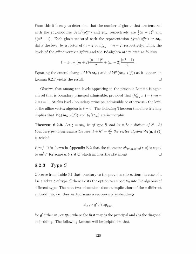
From this it is easy to determine that the number of ghosts that are tensored

with the som-modules Sym2(ρsomω1) and som respectively are 1

2(n − 1)2 and

12(n2 − 1). Each ghost tensored with the representation Sym2(ρsomω1

) or som

shifts the level by a factor of m + 2 or h∨som = m − 2, respectively. Thus, the

levels of the affine vertex algebra and the W-algebra are related as follows

` = kn+ (m+ 2)(n− 1)2

2+ (m− 2)

(n2 − 1)

2.

Equating the central charge of V `(som) and of Wk(soN , ι(f)) as it appears in

Lemma 6.2.7 yields the result.

Observe that among the levels appearing in the previous Lemma is again

a level that is boundary principal admissible, provided that (h∨soN , n) = (mn−

2, n) = 1. At this level - boundary principal admissible or otherwise - the level

of the affine vertex algebra is ` = 0. The following Theorem therefore trivially

implies that Wk(soN , ι(f)) and V`(som) are isomorphic.

Theorem 6.2.9. Let g = soN be of type B and let n be a divisor of N . At

boundary principal admissible level k+ h∨ = h∨

nthe vertex algebra Wk(g, ι(f))

is trivial.

Proof. It is shown in Appendix B.2 that the character chWk(g,ι(f))(τ, z) is equal

to aqbuc for some a, b, c ∈ C which implies the statement.

6.2.3 Type C

Observe from Table 6.1 that, contrary to the previous subsections, in case of a

Lie algebra g of type C there exists the option to embed sl2 into Lie algebras of

different type. The next two subsections discuss implications of these different

embeddings, i.e. they each discuss a sequence of embeddings

sl2 → g′ι→ sp2mn

for g′ either son or sp2n where the first map is the principal and ι is the diagonal

embedding. The following Lemma will be helpful for that.

128

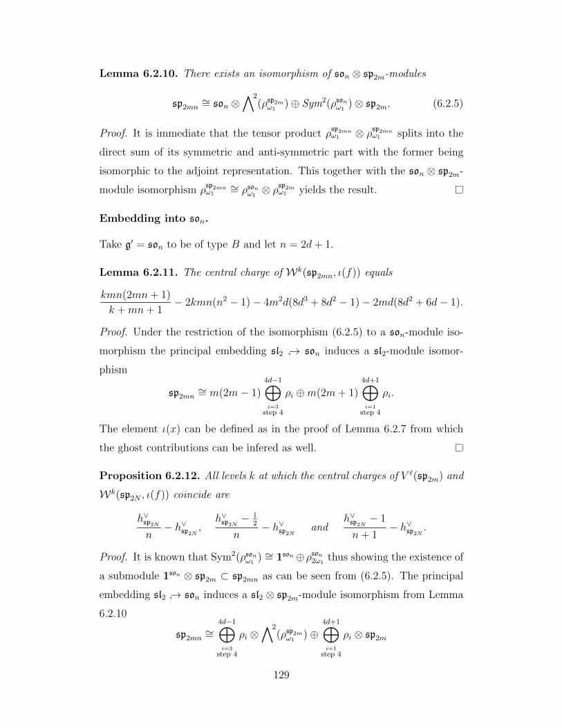
Lemma 6.2.10. There exists an isomorphism of son ⊗ sp2m-modules

sp2mn∼= son ⊗

∧2(ρsp2mω1

)⊕ Sym2(ρsonω1)⊗ sp2m. (6.2.5)

Proof. It is immediate that the tensor product ρsp2mnω1 ⊗ ρsp2mn

ω1 splits into the

direct sum of its symmetric and anti-symmetric part with the former being

isomorphic to the adjoint representation. This together with the son ⊗ sp2m-

module isomorphism ρsp2mnω1

∼= ρsonω1⊗ ρsp2m

ω1 yields the result.

Embedding into son.

Take g′ = son to be of type B and let n = 2d+ 1.

Lemma 6.2.11. The central charge of Wk(sp2mn, ι(f)) equals

kmn(2mn+ 1)

k +mn+ 1− 2kmn(n2 − 1)− 4m2d(8d3 + 8d2 − 1)− 2md(8d2 + 6d− 1).

Proof. Under the restriction of the isomorphism (6.2.5) to a son-module iso-

morphism the principal embedding sl2 → son induces a sl2-module isomor-

phism

sp2mn∼= m(2m− 1)

4d−1⊕i=3

step 4

ρi ⊕m(2m+ 1)4d+1⊕i=1

step 4

ρi.

The element ι(x) can be defined as in the proof of Lemma 6.2.7 from which

the ghost contributions can be infered as well.

Proposition 6.2.12. All levels k at which the central charges of V `(sp2m) and

Wk(sp2N , ι(f)) coincide are

h∨sp2N

n− h∨sp2N

,h∨sp2N

− 12

n− h∨sp2N

andh∨sp2N

− 1

n+ 1− h∨sp2N

.

Proof. It is known that Sym2(ρsonω1) ∼= 1son⊕ρson2ω1

thus showing the existence of

a submodule 1son ⊗ sp2m ⊂ sp2mn as can be seen from (6.2.5). The principal

embedding sl2 → son induces a sl2 ⊗ sp2m-module isomorphism from Lemma

6.2.10

sp2mn∼=

4d−1⊕i=3

step 4

ρi ⊗∧2

(ρsp2mω1

)⊕4d+1⊕i=1

step 4

ρi ⊗ sp2m

129

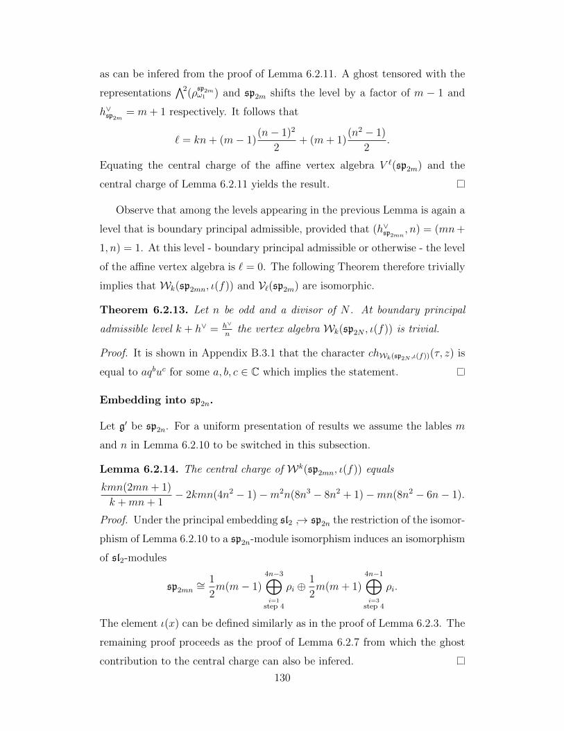
as can be infered from the proof of Lemma 6.2.11. A ghost tensored with the

representations∧2(ρ

sp2mω1 ) and sp2m shifts the level by a factor of m − 1 and

h∨sp2m= m+ 1 respectively. It follows that

` = kn+ (m− 1)(n− 1)2

2+ (m+ 1)

(n2 − 1)

2.

Equating the central charge of the affine vertex algebra V `(sp2m) and the

central charge of Lemma 6.2.11 yields the result.

Observe that among the levels appearing in the previous Lemma is again a

level that is boundary principal admissible, provided that (h∨sp2mn, n) = (mn+

1, n) = 1. At this level - boundary principal admissible or otherwise - the level

of the affine vertex algebra is ` = 0. The following Theorem therefore trivially

implies that Wk(sp2mn, ι(f)) and V`(sp2m) are isomorphic.

Theorem 6.2.13. Let n be odd and a divisor of N . At boundary principal

admissible level k + h∨ = h∨

nthe vertex algebra Wk(sp2N , ι(f)) is trivial.

Proof. It is shown in Appendix B.3.1 that the character chWk(sp2N ,ι(f))(τ, z) is

equal to aqbuc for some a, b, c ∈ C which implies the statement.

Embedding into sp2n.

Let g′ be sp2n. For a uniform presentation of results we assume the lables m

and n in Lemma 6.2.10 to be switched in this subsection.

Lemma 6.2.14. The central charge of Wk(sp2mn, ι(f)) equals

kmn(2mn+ 1)

k +mn+ 1− 2kmn(4n2 − 1)−m2n(8n3 − 8n2 + 1)−mn(8n2 − 6n− 1).

Proof. Under the principal embedding sl2 → sp2n the restriction of the isomor-

phism of Lemma 6.2.10 to a sp2n-module isomorphism induces an isomorphism

of sl2-modules

sp2mn∼=

1

2m(m− 1)

4n−3⊕i=1

step 4

ρi ⊕1

2m(m+ 1)

4n−1⊕i=3

step 4

ρi.

The element ι(x) can be defined similarly as in the proof of Lemma 6.2.3. The

remaining proof proceeds as the proof of Lemma 6.2.7 from which the ghost

contribution to the central charge can also be infered.

130

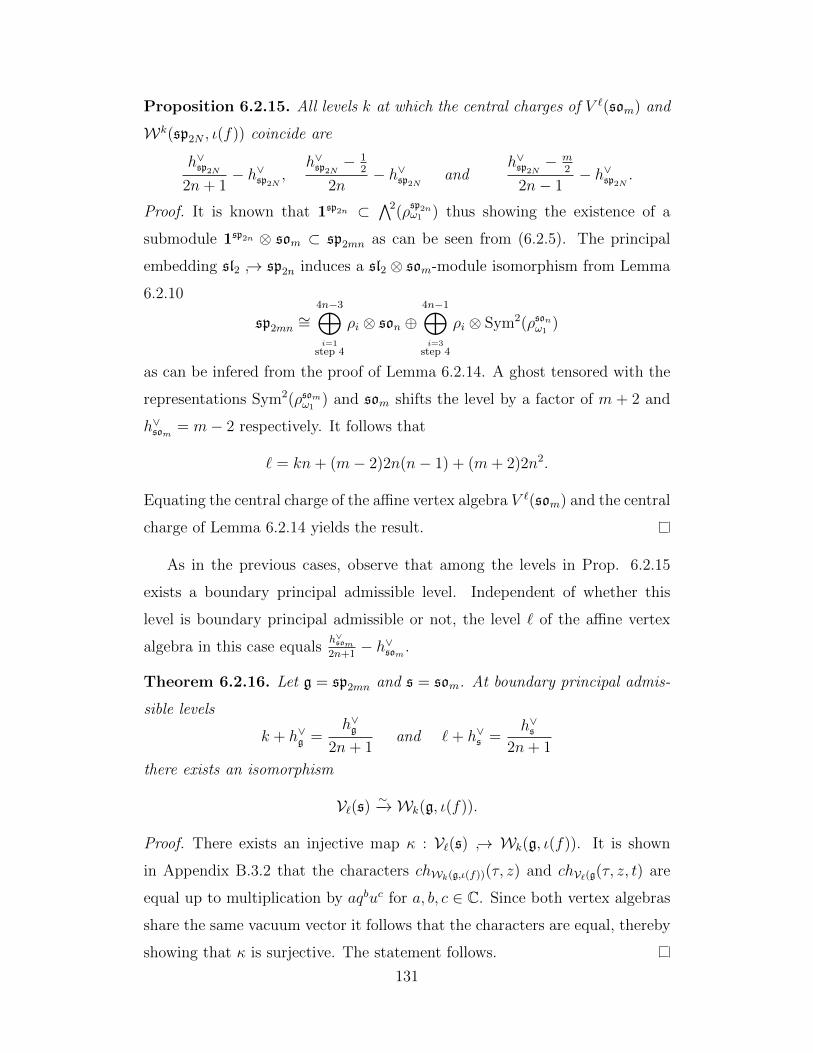
Proposition 6.2.15. All levels k at which the central charges of V `(som) and

Wk(sp2N , ι(f)) coincide are

h∨sp2N

2n+ 1− h∨sp2N

,h∨sp2N

− 12

2n− h∨sp2N

andh∨sp2N

− m2

2n− 1− h∨sp2N

.

Proof. It is known that 1sp2n ⊂∧2(ρ

sp2nω1 ) thus showing the existence of a

submodule 1sp2n ⊗ som ⊂ sp2mn as can be seen from (6.2.5). The principal

embedding sl2 → sp2n induces a sl2 ⊗ som-module isomorphism from Lemma

6.2.10

sp2mn∼=

4n−3⊕i=1

step 4

ρi ⊗ son ⊕4n−1⊕i=3

step 4

ρi ⊗ Sym2(ρsonω1)

as can be infered from the proof of Lemma 6.2.14. A ghost tensored with the

representations Sym2(ρsomω1) and som shifts the level by a factor of m + 2 and

h∨som = m− 2 respectively. It follows that

` = kn+ (m− 2)2n(n− 1) + (m+ 2)2n2.

Equating the central charge of the affine vertex algebra V `(som) and the central

charge of Lemma 6.2.14 yields the result.

As in the previous cases, observe that among the levels in Prop. 6.2.15

exists a boundary principal admissible level. Independent of whether this

level is boundary principal admissible or not, the level ` of the affine vertex

algebra in this case equalsh∨som2n+1

− h∨som .

Theorem 6.2.16. Let g = sp2mn and s = som. At boundary principal admis-

sible levels

k + h∨g =h∨g

2n+ 1and `+ h∨s =

h∨s2n+ 1

there exists an isomorphism

V`(s)∼−→Wk(g, ι(f)).

Proof. There exists an injective map κ : V`(s) → Wk(g, ι(f)). It is shown

in Appendix B.3.2 that the characters chWk(g,ι(f))(τ, z) and chV`(g(τ, z, t) are

equal up to multiplication by aqbuc for a, b, c ∈ C. Since both vertex algebras

share the same vacuum vector it follows that the characters are equal, thereby

showing that κ is surjective. The statement follows.

131

6.2.4 Type D

We now look at the sequence of embeddings

sl2 → sp2n

ι→ so4mn

where the first map is the principal and ι is the diagonal embedding.

Lemma 6.2.17. There exists an isomorphism of sp2n ⊗ sp2m-modules

so4mn∼= sp2n ⊗

∧2(ρsp2mω1

)⊕∧2

(ρsp2nω1

)⊗ sp2m.

Proof. It is immediate that the tensor product ρso4mnω1

⊗ ρso4mnω1

decomposes

into a direct sum of its symmetric and anti-symmetric part. Knowing that

Sym2(ρsp2nω1 ) ∼= sp2n and using the sp2n ⊗ sp2m-module isomorphism ρso4mn

ω1∼=

ρsp2nω1 ⊗ ρ

sp2mω1 yields the result.

Lemma 6.2.18. The central charge of Wk(so4mn, ι(f)) equals

k2mn(4mn− 1)

k + 4mn− 2−2kmn(4n2−1)−4m2n(8n3−8n2 +1)+2mn(8n2−6n−1).

Proof. Restricting the isomorphism from Lemma 6.2.17 to a sp2n-isomorphism

and using the sl2-module decomposition used in the proof of Lemma 6.2.14

yields the sl2-isomorphism

so4mn∼= m(2m− 1)

4n−1⊕i=3

step 4

ρi ⊕m(2m+ 1)4n−3⊕i=1

step 4

ρi.

The element ι(x) can be defined similarly as in Lemma 6.2.14 and the ghost

contributions can be infered from Lemma 6.2.7.

Proposition 6.2.19. All levels k at which the central charges of V `(sp2m) and

Wk(so4N , ι(f)) coincide are

h∨so4N

2n+ 1− h∨so4N

,h∨so4N

+ 1

2n− h∨so4N

andh∨so4N

− 2m

2n− 1− h∨so4N

.

Proof. Restricting the isomorphism of Lemma 6.2.17 to an sl2 ⊗ sp2m-module

isomorphism under the principal embedding sl2 → sp2n yields

so4mn∼=

4n−1⊕i=3

step 4

ρi ⊗∧2

(ρsp2mω1

)⊕4n−3⊕i=1

step 4

ρi ⊗ sp2m.

132

Ghosts tensored with the representations∧2(ρ

sp2mω1 ) and sp2m contribute a shift

to the level by m− 1 and h∨sp2m= m + 1, respectively. The level of the affine

vertex algebra can be written as

` = kn+ (m− 1)2n2 + (m+ 1)2n(n− 1).

It is known that 1sp2n ⊂∧2(ρ

sp2nω1 ) which shows that there exists a submodule

1sp2n ⊗ sp2m ⊂ so4mn thereby explaining the term kn. Equating the cen-

tral charge of the affine vertex algebra V `(sp2m) with the central charge from

Lemma 6.2.18 yields the result.

Theorem 6.2.20. Let g = so4mn and s = sp2m. At boundary principal ad-

missible levels

k + h∨g =h∨g

2n+ 1and `+ h∨s =

h∨s2n+ 1

there exists an isomorphism

V`(s)∼−→Wk(g, ι(f)).

Proof. There exists an injective map κ : V`(s) → Wk(g, ι(f)). It is shown

in Appendix B.4 that the characters chWk(g,ι(f))(τ, z) and chV`(g(τ, z, t) are

equal up to multiplication by aqbuc for a, b, c ∈ C. Since both vertex algebras

share the same vacuum vector it follows that the characters are equal, thereby

showing that κ is surjective. The statement follows.

133

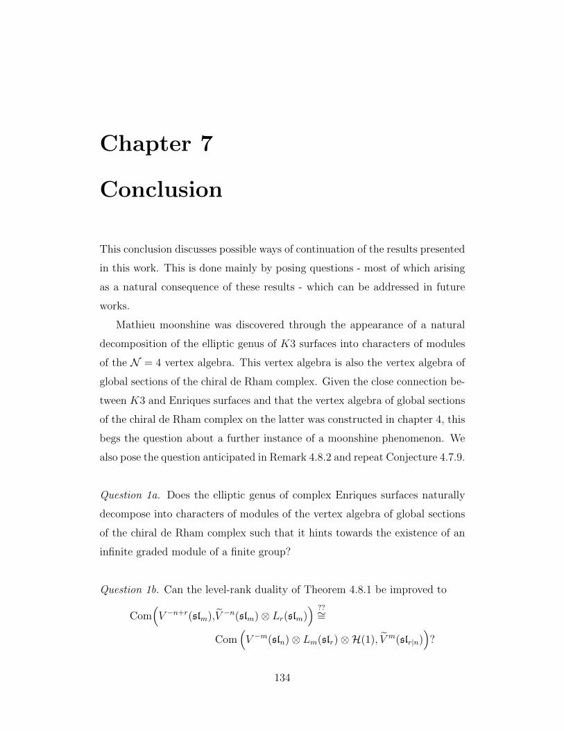
Chapter 7

Conclusion

This conclusion discusses possible ways of continuation of the results presented

in this work. This is done mainly by posing questions - most of which arising

as a natural consequence of these results - which can be addressed in future

works.

Mathieu moonshine was discovered through the appearance of a natural

decomposition of the elliptic genus of K3 surfaces into characters of modules

of the N = 4 vertex algebra. This vertex algebra is also the vertex algebra of

global sections of the chiral de Rham complex. Given the close connection be-

tween K3 and Enriques surfaces and that the vertex algebra of global sections

of the chiral de Rham complex on the latter was constructed in chapter 4, this

begs the question about a further instance of a moonshine phenomenon. We

also pose the question anticipated in Remark 4.8.2 and repeat Conjecture 4.7.9.

Question 1a. Does the elliptic genus of complex Enriques surfaces naturally

decompose into characters of modules of the vertex algebra of global sections

of the chiral de Rham complex such that it hints towards the existence of an

infinite graded module of a finite group?

Question 1b. Can the level-rank duality of Theorem 4.8.1 be improved to

Com(V −n+r(slm),V −n(slm)⊗ Lr(slm)

) ??∼=

Com(V −m(sln)⊗ Lm(slr)⊗H(1), V m(slr|n)

)?

134

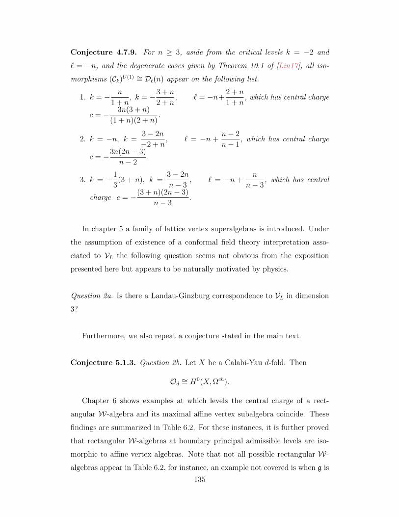
Conjecture 4.7.9. For n ≥ 3, aside from the critical levels k = −2 and

` = −n, and the degenerate cases given by Theorem 10.1 of [Lin17], all iso-

morphisms (Ck)U(1) ∼= D`(n) appear on the following list.

1. k = − n

1 + n, k = −3 + n

2 + n, ` = −n+

2 + n

1 + n, which has central charge

c = − 3n(3 + n)

(1 + n)(2 + n).

2. k = −n, k =3− 2n

−2 + n, ` = −n +

n− 2

n− 1, which has central charge

c = −3n(2n− 3)

n− 2.

3. k = −1

3(3 + n), k =

3− 2n

n− 3, ` = −n +

n

n− 3, which has central

charge c = −(3 + n)(2n− 3)

n− 3.

In chapter 5 a family of lattice vertex superalgebras is introduced. Under

the assumption of existence of a conformal field theory interpretation asso-

ciated to VL the following question seems not obvious from the exposition

presented here but appears to be naturally motivated by physics.

Question 2a. Is there a Landau-Ginzburg correspondence to VL in dimension

3?

Furthermore, we also repeat a conjecture stated in the main text.

Conjecture 5.1.3. Question 2b. Let X be a Calabi-Yau d-fold. Then

Od ∼= H0(X,Ωch).

Chapter 6 shows examples at which levels the central charge of a rect-

angular W-algebra and its maximal affine vertex subalgebra coincide. These

findings are summarized in Table 6.2. For these instances, it is further proved

that rectangular W-algebras at boundary principal admissible levels are iso-

morphic to affine vertex algebras. Note that not all possible rectangular W-

algebras appear in Table 6.2, for instance, an example not covered is when g is

135

of type C and g′ is of type D. With that in mind we pose two general questions.

Question 3a. At what levels does a rectangular W-algebra allow a conformal

embedding of its maximal universal affine sub vertex algebra?

Question 3b. At what levels is the simple quotient of a rectangularW-algebra

isomorphic to the simple quotient of its maximal universal affine sub vertex

algebra?

136

References

[ACKL17] T. Arakawa, T. Creutzig, K. Kawasetsu, and A. R. Linshaw,Orbifolds and cosets of minimalW-algebras, Comm. Math. Phys.355 (2017), 339–372.

[ACL17] T. Arakawa, T. Creutzig, and A. R. Linshaw, Cosets ofBershadsky-Polyakov algebras and rational W-algebras of type A,Sel. Math. New Ser. 23 (2017), 2369–2395.

[ACL19] , W -algebras as coset vertex algebras, Inventiones mathe-maticae 218 (2019), no. 1, 145–195.

[Ada99] D. Adamovic, Representations of the N = 2 superconformal ver-tex algebra, International Mathematics Research Notices 1999(1999), no. 2, 61–79.

[Ada16] , A realization of certain modules for the N = 4 supercon-

formal algebra and the affine Lie algebra A(1)2 , Transformation

Groups 21 (2016), no. 2, 299–327.

[AKM+16] D. Adamovic, V. G. Kac, P. Moseneder Frajria, P. Papi, andO. Perse, Finite vs. Infinite Decompositions in Conformal Em-beddings, Communications in Mathematical Physics 348 (2016),no. 2, 445–473.

[AKM+17] , Conformal embeddings of affine vertex algebras in min-imal W-algebras II: decompositions, Japanese Journal of Mathe-matics 12 (2017), no. 2, 261–315.

[AKM+18a] , An Application of Collapsing Levels to the Representa-tion Theory of Affine Vertex Algebras, International MathematicsResearch Notices (2018), rny237.

[AKM+18b] , Conformal embeddings of affine vertex algebras in min-imal W-algebras I: Structural results, Journal of Algebra 500(2018), 117 – 152, Special Issue dedicated to Efim Zelmanov.

[AL17] M. Al-Ali and A. R. Linshaw, The Z2-orbifold of the W3-algebra,Communications in Mathematical Physics 353 (2017), no. 3,1129–1150.

[Ali99] A. Ali, Classification of Two Dimensional N=4 SuperconformalSymmetries, arXiv e-prints (1999), hep–th/9906096.

137

[AM17] T. Arakawa and A. Molev, Explicit generators in rectangularaffine W-algebras of type A, Letters in Mathematical Physics 107(2017), no. 1, 47–59.

[Ara04] T. Arakawa, Vanishing of cohomology associated to quantizedDrinfeld-Sokolov reduction, International Mathematics ResearchNotices 2004 (2004), no. 15, 729–767.

[Ara05] , Representation theory of superconformal algebras andthe Kac-Roan-Wakimoto conjecture, Duke Math. J. 130 (2005),no. 3, 435–478.

[Ara07] , Representation theory of W-algebras, Inventiones math-ematicae 169 (2007), no. 2, 219–320.

[Ara12] , W-algebras at the critical level, Contemporary Mathe-matics 565 (2012), 1–14.

[BHS08] D. Ben-Zvi, R. Heluani, and M. Szczesny, Supersymmetry of thechiral de Rham complex, Compositio Mathematica 144 (2008),no. 2, 503–521.

[BL00] L. A. Borisov and A. Libgober, Elliptic genera of toric varietiesand applications to mirror symmetry, Inventiones mathematicae140 (2000), no. 2, 453–485.

[BLL+15] C. Beem, M. Lemos, P. Liendo, W. Peelaers, L. Rastelli, andB. C. van Rees, Infinite Chiral Symmetry in Four Dimensions,Commun. Math. Phys. 336 (2015), 1359–1433.

[BMR19] F. Bonetti, C. Meneghelli, and L. Rastelli, VOAs labelled by com-plex reflection groups and 4d SCFTs, Journal of High EnergyPhysics 05 (2019), 155.

[Bor86] R. E. Borcherds, Vertex algebras, Kac-Moody algebras, and theMonster, Proceedings of the National Academy of Sciences 83(1986), no. 10, 3068–3071.

[Bor92] , Monstrous moonshine and monstrous Lie superalgebras,Inventiones mathematicae 109 (1992), no. 1, 405–444.

[Bor01] L. A. Borisov, Vertex Algebras and Mirror Symmetry, Communi-cations in Mathematical Physics 215 (2001), 517–557.

[CDD+15] M. C. N. Cheng, X. Dong, J. F. R. Duncan, S. Harrison,S. Kachru, and T. Wrase, Mock modular Mathieu moonshine mod-ules, Research in the Mathematical Sciences 2 (2015), no. 1, 13.

[CDH14a] M. C. N. Cheng, J. F. R. Duncan, and J. A. Harvey, Umbralmoonshine, Communications in Number Theory and Physics 8(2014), no. 2, 101 – 242.

[CDH14b] , Umbral moonshine and the Niemeier lattices, Researchin the Mathematical Sciences 1 (2014), no. 1, 3.

138

[CDHK17] M. C. N. Cheng, J. F. R. Duncan, S. M. Harrison, and S. Kachru,Equivariant K3 invariants, Communications in Number Theoryand Physics 11 (2017), no. 1.

[CDR17] T. Creutzig, J. F. R. Duncan, and W. Riedler, Self-dual vertexoperator superalgebras and superconformal field theory, Journalof Physics A: Mathematical and Theoretical 51 (2017), no. 3,034001.

[CFL19] T. Creutzig, B. Feigin, and A. R. Linshaw, N = 4 super-conformal algebras and diagonal cosets, arXiv e-prints (2019),arXiv:1910.01228.

[CG17] T. Creutzig and D. Gaiotto, Vertex Algebras for S-duality, arXive-prints (2017), arXiv:1708.00875.

[CGL18] T. Creutzig, D. Gaiotto, and A. R. Linshaw, S-duality for thelarge N = 4 superconformal algebra, arXiv e-prints (2018),arXiv:1804.09821.

[CH14] T. Creutzig and G. Hohn, Mathieu moonshine and the geometryof K3 surfaces, Communications in Number Theory and Physics8 (2014), no. 2, 295 – 328.

[CH19a] T. Creutzig and Y. Hikida, Rectangular W-algebras, extendedhigher spin gravity and dual coset CFTs, Journal of High EnergyPhysics 2019 (2019), no. 2, 147.

[CH19b] , Rectangular W -(super)algebras and their representa-tions, arXiv e-prints (2019), arXiv:1906.05868.

[Che10] M. C. N. Cheng, K3 Surfaces, N=4 Dyons, and the MathieuGroup M24, Commun. Num. Theor. Phys. 4 (2010).

[CHKW15] M. C. N. Cheng, S. M. Harrison, S. Kachru, and D. Whalen,Exceptional Algebra and Sporadic Groups at c=12, arXiv e-prints(2015), arXiv:1503.07219.

[CHU19] T. Creutzig, Y. Hikida, and T. Uetoko, Rectangular W-algebrasof types so(M) and sp(2M) and dual coset CFTs, arXiv e-prints(2019), arXiv:1906.05872.

[CHVZ18] M. C. N. Cheng, S. M. Harrison, R. Volpato, and M. Zimet, K3string theory, lattices and moonshine, Research in the Mathemat-ical Sciences 5 (2018), no. 3, 32.

[CKL19] T. Creutzig, S. Kanade, and A. R. Linshaw, Simple current exten-sions beyond semi-simplicity, Communications in ContemporaryMathematics (2019), 1950001, arXiv:1511.08754.

[CKLR19] T. Creutzig, S. Kanade, A. R. Linshaw, and D. Ridout, Schur-Weyl duality for Heisenberg cosets, Transformation Groups 24(2019), no. 2, 301–354.

139

[CKM17] T. Creutzig, S. Kanade, and R. McRae, Tensor categories forvertex operator superalgebra extensions, arXiv e-prints (2017),arXiv:1705.05017.

[CL13] T. Creutzig and A. R. Linshaw, A commutant realization ofOdake’s algebra, Transformation Groups 18 (2013), no. 3, 615–637.

[CL18] , Cosets of the W k(sl4, fsubreg)-algebra , Contemp. Math.711 (2018), 105–117.

[CL19] , Cosets of affine vertex algebras inside larger structures,Journal of Algebra 517 (2019), 396–438.

[CLR19] T. Creutzig, A. R. Linshaw, and W. Riedler, Invariant subalge-bras of the small N = 4 superconformal algebra, arXiv e-prints(2019), arXiv:1910.02033.

[CN79] J. H. Conway and S. P. Norton, Monstrous Moonshine, Bulletinof the London Mathematical Society 11 (1979), no. 3, 308–339.

[Con68] J. H. Conway, A Perfect Group of Order8,315,553,613,086,720,000 and the Sporadic Simple Groups,Proceedings of the National Academy of Sciences of the UnitedStates of America 61 (1968), no. 2, 398–400.

[Con69] , A Group of Order 8,315,553,613,086,720,000, Bulletinof the London Mathematical Society 1 (1969), no. 1, 79–88.

[CR13] T. Creutzig and D. Ridout, Modular data and Verlinde formu-lae for fractional level WZW models II, Nuclear Physics B 875(2013), no. 2, 423 – 458.

[Cre17] T. Creutzig, W-algebras for Argyres–Douglas theories, EuropeanJournal of Mathematics 3 (2017), 659–690.

[Cre18] , Logarithmic W-algebras and Argyres-Douglas theories athigher rank, Journal of High Energy Physics 2018 (2018), 188.

[CS88] J. H. Conway and N. Sloane, Sphere Packings, Lattices andGroups, Grundlehren der mathematischen Wissenschaften, vol.290, Springer-Verlag New York, 1988.

[DGO15a] J. F. R. Duncan, M. J. Griffin, and K. Ono, Moonshine, Researchin the Mathematical Sciences 2 (2015), no. 1, 11.

[DGO15b] , Proof of the umbral moonshine conjecture, Research inthe Mathematical Sciences 2 (2015), no. 1, 26.

[DLM96] C. Dong, H. Li, and G. Mason, Compact automorphism groupsof vertex operator algebras, International Mathematics ResearchNotices 1996 (1996), no. 18, 913–921.

[DLM98] , Twisted representations of vertex operator algebras,Mathematische Annalen 310 (1998), no. 3, 571–600.

140

[DLM00] , Modular-Invariance of Trace Functions in Orbifold The-ory and Generalized Moonshine, Communications in Mathemat-ical Physics 214 (2000), no. 1, 1–56.

[DLMM98] C. Dong, H. Li, G. Mason, and P. S. Montague, The radical of avertex operator algebra, The Monster and Lie Algebras: Proceed-ings of a Special Research Quarter at the Ohio State University(J. Ferrar and K. Harada, eds.), De Gruyter, 1998, p. 17–26.

[DM94] C. Dong and G. Mason, Nonabelian orbifolds and the boson-fermion correspondence, Comm. Math. Phys. 163 (1994), no. 3,523–559.

[DM02] , Rational Vertex Operator Algebras and the Effective Cen-tral Charge, International Mathematics Research Notices (2002).

[DM06] , Integrability of C2-cofinite vertex operator algebras, In-ternational Mathematics Research Notices 2006 (2006).

[DM15] J. F. R. Duncan and S. Mack-Crane, The moonshine module forConway’s largest group, Forum of Mathematics, Sigma 3 (2015),e10.

[DM16] , Derived equivalences of K3 surfaces and twined ellipticgenera, Research in the Mathematical Sciences 3 (2016), no. 1,1.

[DMO17] J. F. R. Duncan, M. H. Mertens, and K. Ono, O’Nan moonshineand arithmetic, arXiv e-prints (2017), arXiv:1702.03516.

[DN99] C. Dong and K. Nagatomo, Classification of Irreducible Modulesfor the Vertex Operator Algebra M(1)+, Journal of Algebra 216(1999), no. 1, 384 – 404.

[Dun07] J. F. R. Duncan, Super-moonshine for Conway’s largest sporadicgroup, Duke Math. J. 139 (2007), no. 2, 255–315.

[DW10] C. Dong and Q. Wang, The Structure of Parafermion Vertex Op-erator Algebras: General Case, Communications in MathematicalPhysics 299 (2010), no. 3, 783–792.

[DY93] P. Di Francesco and S. Yankielowicz, Ramond sector charactersand N = 2 Landau-Ginzburg models, Nuclear Physics B 409(1993), no. 1, 186 – 210.

[DZ05] C. Dong and Z. Zhao, Modularity in Orbifold Theory for Ver-tex Operator Superalgebras, Communications in MathematicalPhysics 260 (2005), no. 1, 227–256.

[DZ10] , Modularity of Trace Functions in Orbifold Theory forZ-Graded Vertex Operator Superalgebras, Moonshine - The FirstQuarter Century and Beyond: Proceedings of a Workshop on theMoonshine Conjectures and Vertex Algebras (James Lepowsky,John McKay, and Michael P.Editors Tuite, eds.), London Mathe-matical Society Lecture Note Series, Cambridge University Press,2010, p. 128–143.

141

[EH11] T. Eguchi and K. Hikami, Note on twisted elliptic genus of K3surface, Physics Letters B 694 (2011), no. 4, 446 – 455.

[EHKZ13] J. Ekstrand, R. Heluani, J. Kallen, and M. Zabzine, Chiral deRham Complex on Riemannian Manifolds and Special Holonomy,Communications in Mathematical Physics 318 (2013), no. 3, 575–613.

[EOT11] T. Eguchi, H. Ooguri, and Y. Tachikawa, Notes on the K3 Surfaceand the Mathieu Group M24, Experiment. Math. 20 (2011), no. 1,91–96.

[EOTY89] T. Eguchi, H. Ooguri, A. Taormina, and S.-K. Yang, Superconfor-mal algebras and string compactification on manifolds with SU(n)holonomy, Nuclear Physics B 315 (1989), no. 1, 193 – 221.

[ET87] T. Eguchi and A. Taormina, Unitary representations of the N=4superconformal algebra, Physics Letters B 196 (1987), no. 1, 75– 81.

[ET88a] , Character formulas for the N = 4 superconformal alge-bra, Physics Letters B 200 (1988), no. 3, 315 – 322.

[ET88b] , On the unitary representations of N = 2 and N = 4superconformal algebras, Physics Letters B 210 (1988), no. 1,125 – 132.

[FB04] E. Frenkel and D. Ben-Zvi, Vertex Algebras and Algebraic Curves,Mathematical surveys and monographs, American MathematicalSociety, 2004.

[FF90] B. Feigin and E. Frenkel, Quantization of the Drinfeld-SokolovReduction, Physics Letters B 246 (1990), no. 1, 75 – 81.

[FHL93] I. Frenkel, Y.Z. Huang, and J. Lepowsky, On Axiomatic Ap-proaches to Vertex Operator Algebras and Modules, AmericanMathematical Society: Memoirs of the American MathematicalSociety, no. 494, American Mathematical Society, 1993.

[FKW92] E. Frenkel, V. G. Kac, and M. Wakimoto, Characters and fusionrules for W -algebras via quantized Drinfel’d-Sokolov reduction,Comm. Math. Phys. 147 (1992), no. 2, 295–328.

[FL88] V. A. Fateev and S. L. Lukyanov, The Models of Two-Dimensional Conformal Quantum Field Theory with Z(n) Sym-metry, Int. J. Mod. Phys. A3 (1988), 507.

[FLM84] I. B. Frenkel, J. Lepowsky, and A. Meurman, A natural represen-tation of the Fischer-Griess Monster with the modular functionJ as character, Proceedings of the National Academy of Sciences81 (1984), no. 10, 3256–3260.

[FLM85] , A Moonshine Module for the Monster, Vertex Oper-ators in Mathematics and Physics (New York, NY) (J. Lep-owsky, S. Mandelstam, and I. M. Singer, eds.), Springer US, 1985,pp. 231–273.

142

[FLM89] , Vertex Operator Algebras and the Monster, Pure andApplied Mathematics, Elsevier Science, 1989.

[Fre81] I. B. Frenkel, Two constructions of affine Lie algebra representa-tions and boson-fermion correspondence in quantum field theory,Journal of Functional Analysis 44 (1981), no. 3, 259 – 327.

[FRS02] J. Fuchs, I. Runkel, and C. Schweigert, TFT construction ofRCFT correlators I: partition functions, Nuclear Physics B 646(2002), no. 3, 353 – 497.

[FS07] E. Frenkel and M. Szczesny, Chiral de Rham Complex and Orb-ifolds, J. Algebraic Geom. 16 (2007), 599–624.

[FST98] B. L. Feigin, A. M. Semikhatov, and I. Yu. Tipunin, Equivalencebetween chain categories of representations of affine sl(2) andN = 2 superconformal algebras, Journal of Mathematical Physics39 (1998), 3865–3905.

[Gab00] M. Gaberdiel, An introduction to conformal field theory, Reportson Progress in Physics 63 (2000), no. 4, 607–667.

[Gan16] T. Gannon, Much ado about Mathieu, Advances in Mathematics301 (2016), 322 – 358.

[Gen17] N. Genra, Screening operators for W-algebras, Selecta Mathe-matica 23 (2017), no. 3, 2157–2202.

[GHV10a] M. R. Gaberdiel, S. Hohenegger, and R. Volpato, Mathieu Moon-shine in the elliptic genus of K3, Journal of High Energy Physics2010 (2010), no. 10, 62.

[GHV10b] , Mathieu twining characters for K3, Journal of High En-ergy Physics 2010 (2010), no. 9, 58.

[GHV12] , Symmetries of K3 sigma models, Communications inNumber Theory and Physics 6 (2012), no. 1, 1 – 50.

[GKH17] M. R. Gaberdiel, C. A. Keller, and P. Hynek, Mathieu Moonshineand symmetry surfing, Journal of Physics A: Mathematical andTheoretical 50 (2017), no. 47, 474002.

[GM16] M. J. Griffin and M. H. Mertens, A proof of the Thompson moon-shine conjecture, Research in the Mathematical Sciences 3 (2016),no. 1, 36.

[Gri00] V. Gritsenko, Elliptic genus of Calabi-Yau manifolds and Jacobiand Siegel modular forms., St. Petersbg. Math. J. 11 (2000),no. 5, 781–804 (2000); and algebra anal. 11, no. 5, 100–125 (En-glish).

[GS88] P. Goddard and A. Schwimmer, Factoring out free fermions andsuperconformal algebras, Physics Letters B 214 (1988), no. 2, 209– 214.

143

[GTVW14] M. R. Gaberdiel, A. Taormina, R. Volpato, and K. Wendland, AK3 sigma model with Z8

2 : M20 symmetry, Journal of High EnergyPhysics 2014 (2014), no. 2, 22.

[GW09] R. Goodman and N.R. Wallach, Symmetry, Representations, andInvariants, Graduate Texts in Mathematics, Springer New York,2009.

[HA15] J. Han and C. Ai, Three equivalent rationalities of vertex operatorsuperalgebras, Journal of Mathematical Physics 56 (2015), no. 11,111701.

[Hel09] R. Heluani, Supersymmetry of the Chiral de Rham Complex 2:Commuting Sectors, International Mathematics Research Notices2009 (2009), no. 6, 953–987.

[Hir78] F Hirzebruch, Topological Methods in Algebraic Geometry,Grundlehren der mathematischen Wissenschaften, vol. 131,Springer, Berlin-Heidelberg-New York, 1978.

[Hoh91] G. Hohn, Komplexe elliptische Geschlechter und S1-aquivarianteKobordismustheorie, Master’s thesis, Bonn, 1991, arXiv e-prints(2004), arXiv: math/0405232.

[Hoh07] , Selbstduale vertexoperatorsuperalgebren und das baby-monster (Self-dual vertex operator super algebras and the babymonster), Bonner Mathematische Schriften 286 (2007), 1–85.

[HR16] J. A. Harvey and B. C. Rayhaun, Traces of singular moduli andmoonshine for the Thompson group, Communications in NumberTheory and Physics 10 (2016), no. 1, 23 – 62.

[Hua92] Y.-Z. Huang, Vertex Operator Algebras and Conformal Field The-ory, International Journal of Modern Physics A 07 (1992), no. 10,2109–2151.

[Kac98] V. G. Kac, Vertex Algebras for Beginners, University lecture se-ries, American Mathematical Society, 1998.

[Kap05] A. Kapustin, Chiral de Rham complex and the half-twisted sigma-model, arXiv e-prints (2005), arXiv:hep–th/0504074.

[KKPT16] S. Katz, A. Klemm, R. Pandharipande, and R. P. Thomas, On theMotivic Stable Pairs Invariants of K3 Surfaces, K3 Surfaces andTheir Moduli (C. Faber, G. Farkas, and G. van der Geer, eds.),Springer International Publishing, Cham, 2016, pp. 111–146.

[KKV99] S. Katz, A. Klemm, and C. Vafa, M-Theory, topological stringsand spinning black holes, Advances in Theoretical and Mathe-matical Physics 3 (1999), no. 5, 1–76 (English (US)).

[KM15] M. Krauel and M. Miyamoto, A modular invariance property ofmultivariable trace functions for regular vertex operator algebras,Journal of Algebra 444 (2015), 124 – 142.

144

[KO03] A. Kapustin and D. Orlov, Vertex Algebras, Mirror Symmetry,and D-Branes: The Case of Complex Tori, Communications inMathematical Physics 233 (2003), 79–136.

[KR96] V. Kac and A. Radul, Representation theory of the vertex algebraW1+∞, Transformation Groups 1 (1996), no. 1, 41–70.

[Kri90] I. M. Krichever, Generalized elliptic genera and baker-Akhiezerfunctions, Mathematical notes of the Academy of Sciences of theUSSR 47 (1990), no. 2, 132–142.

[KRW03] V. Kac, S.-S. Roan, and M. Wakimoto, Quantum Reduction forAffine Superalgebras, Communications in Mathematical Physics241 (2003), no. 2-3, 307–342.

[KT17] S. Kachru and A. Tripathy, The Hodge-Elliptic Genus, SpinningBPS States, and Black Holes, Communications in MathematicalPhysics 355 (2017), no. 1, 245–259.

[KW04] V. G. Kac and M. Wakimoto, Quantum reduction and representa-tion theory of superconformal algebras, Advances in Mathematics185 (2004), no. 2, 400 – 458.

[KW05] , Corrigendum to “Quantum reduction and representa-tion theory of superconformal algebras”: [Adv. Math. 185 (2004)400–458], Advances in Mathematics 193 (2005), 453–455.

[KW17] , A remark on boundary level admissible representations,Comptes Rendus Mathematique 355 (2017), no. 2, 128 – 132.

[Lan88] P. Landweber (ed.), Elliptic Curves and Modular Forms inAlgebraic Topology, Lecture Notes in Mathematics, vol. 1326,Springer, 1988.

[Li04] H. Li, Vertex algebras and vertex Poisson algebras, Communica-tions in Contemporary Mathematics 06 (2004), no. 01, 61–110.

[Lin13] A. R. Linshaw, Invariant subalgebras of affine vertex algebras,Advances in Mathematics 234 (2013), 61 – 84.

[Lin17] , Universal two-parameterW∞-algebra and vertex algebrasof type W(2, 3, . . . , N), arXiv e-prints (2017), arXiv:1710.02275.

[LL04] J. Lepowsky and H. Li, Introduction to Vertex Operator Algebrasand Their Representations, Progress in mathematics, Birkhauser,2004.

[LL07] B. H. Lian and A. R. Linshaw, Howe Pairs in the Theory ofVertex Algebras, J. Algebra 317 (2007), 111–152.

[LSS15] A. R. Linshaw, G. W. Schwarz, and B. Song, Arc spaces andthe vertex algebra commutant problem, Advances in Mathematics277 (2015), 338 – 364.

145

[LVW89] W. Lerche, C. Vafa, and N. P. Warner, Chiral rings in N = 2superconformal theories, Nuclear Physics B 324 (1989), no. 2,427 – 474.

[LZ95] Bong H. Lian and Gregg J. Zuckerman, Commutative quantumoperator algebras, Journal of Pure and Applied Algebra 100(1995), no. 1, 117 – 139.

[Mal99] J. M. Maldacena, The Large N limit of superconformal field the-ories and supergravity, Int. J. Theor. Phys. 38 (1999), no. 4,1113–1133.

[MS99a] F. Malikov and V. Schechtman, Chiral de Rham complex. II, Dif-ferential Topology, Infinite-Dimensional Lie Algebras, and Ap-plications: D. B. Fuchs’ 60th Anniversary Collection (AlexanderAstashkevich and Serge Tabachnikov, eds.), American Mathe-matical Society, 1999, pp. 149–188.

[MS99b] , Chiral Poincare duality, Math. Res. Lett. 6 (1999), 533.

[MS03] , Deformations of Vertex Algebras, Quantum Cohomologyof Toric Varieties, and Elliptic Genus, Communications in Math-ematical Physics 234 (2003), no. 1, 77–100.

[MSV99] F. Malikov, V. Schechtman, and A. Vaintrob, Chiral de RhamComplex, Communications in Mathematical Physics 204 (1999),no. 2, 439–473.

[NW01] W. Nahm and K. Wendland, A Hiker’s Guide to K3. Aspects ofN = (4,4) Superconformal Field Theory with Central Charge c =6, Communications in Mathematical Physics 216 (2001), 85–138.

[Oda90] S. Odake, c=3d conformal algebra with extended Supersymmetry,Modern Physics Letters A 5 (1990), no. 8, 561–580.

[OS14] V. Ostrik and M. Sun, Level-Rank Duality via Tensor Categories,Communications in Mathematical Physics 326 (2014), no. 1, 49–61.

[PT16] R. Pandharipande and R. P. Thomas, The Katz-Klemm-Vafa con-jecture for K3 surfaces, Forum of Mathematics, Pi 4 (2016), e4.

[Ran77] R. A. Rankin, Modular forms and functions, Cambridge Univer-sity Press, 1977.

[RY87] F. Ravanini and S.-K. Yang, Modular invariance in N=2 super-conformal field theories, Physics Letters B 195 (1987), no. 2, 202– 208.

[Son15] B. Song, The Global Sections of the Chiral de Rham Complex ona Kummer Surface, International Mathematics Research Notices2016 (2015), no. 14, 4271–4296.

[Son16] , Vector bundles induced from jet schemes, arXiv e-prints(2016), arXiv:1609.03688.

146

[Son18] , The global sections of chiral de Rham complexes oncompact Ricci-flat Kahler manifolds, arXiv e-prints (2018),arXiv:1809.10320.

[Tam99] H. Tamanoi, Symmetric invariant pairings in vertex operator su-per algebras and Gramians, Journal of Pure and Applied Algebra140 (1999), no. 2, 149 – 189.

[Thi91] K. Thielemans, A MathematicaTM Package for computing Opera-tor Product Expansions, International Journal of Modern PhysicsC 02 (1991), 787.

[Tho79a] J. G. Thompson, Finite Groups and Modular Functions, Bulletinof the London Mathematical Society 11 (1979), no. 3, 347–351.

[Tho79b] , Some Numerology between the Fischer-Griess Monsterand the Elliptic Modular Function, Bulletin of the London Math-ematical Society 11 (1979), no. 3, 352–353.

[TW13] A. Taormina and K. Wendland, The overarching finite symmetrygroup of Kummer surfaces in the Mathieu group M24, Journal ofHigh Energy Physics 08 (2013), 125.

[TW15a] , A twist in the M24 moonshine story, Confluentes Math-ematici 7 (2015), no. 1, 83–113 (en).

[TW15b] , Symmetry-surfing the moduli space of Kummer K3s,Proc. Symp. Pure Math. 90 (2015), 129–154.

[TW17] , The Conway Moonshine Module is a Reflected K3 The-ory, arXiv e-prints (2017), arXiv:1704.03813.

[TZZ99] H. Tamanoi, I.N.E. Zhuzhoma, and E.V. Zhuzhoma, Elliptic Gen-era and Vertex Operator Super-Algebras, Elliptic Genera and Ver-tex Operator Super-algebras, no. no. 1704, Springer, 1999.

[Van13] J. Van Ekeren, Modular Invariance for Twisted Modules over aVertex Operator Superalgebra, Communications in MathematicalPhysics 322 (2013), no. 2, 333–371.

[Vol14] R. Volpato, On symmetries of N = (4, 4) sigma models on T 4,Journal of High Energy Physics 08 (2014), 094.

[Wen15] K. Wendland, Snapshots of Conformal Field Theory, Mathe-matical Aspects of Quantum Field Theories (D. Calaque andT. Strobl, eds.), Springer International Publishing, Cham, 2015,pp. 89–129.

[Wen19] , Hodge-Elliptic Genera and How They Govern K3 Theo-ries, Communications in Mathematical Physics 368 (2019), no. 1,187–221.

[Wey46] H. Weyl, The Classical Groups: Their Invariants and Represen-tations, Princeton University Press, 1946.

147

[Wit87] E. Witten, Elliptic genera and quantum field theory, Commun.Math. Phys. 109 (1987), 525–536.

[Wit94] , On the Landau-Ginzburg description of N=2 minimalmodels, Int. J. Mod. Phys. A9 (1994), 4783–4800.

[Zhu96] Y. Zhu, Modular Invariance of Characters of Vertex Operator Al-gebras, Journal of the American Mathematical Society 9 (1996),no. 1, 237–302.

148

Appendix A

Decoupling relations andsingular fields

A.1 Decoupling relations

For the convenience of the reader we repeat the chosen conventions.

Q+ = G−,2 Q− = G+,1

G+ = G+,2 G− = G−,1

Un,0 =: ∂nJ+J− : Vn,0 =: ∂nG+G− :

An,0 =: ∂nJ+G− : Bn,0 =: ∂nJ−G+ :

Σ(0)±2n,0 =: ∂2nJ±J± : , Σ

(1)±n,0 =: ∂nJ±G± : , Σ

(2)±2n+1,0 =: ∂2n+1G±G± :

All relations below were verified by computer [Thi91]. Note that applying the

automorphism θ specified in the proof of Theorem 4.5.4 on the decoupling

relation for Σ(1)+2,0 (see A.1.2) yields a decoupling relation for Σ

(1)−2,0 that holds

149

at all levels k 6= 4.

0 =k

3U3,0 −

k

2V2,0 + ∂U2,0 −

1

2: U2,0J : + (1 + k) ∂V1,0+ : V1,0J :

− : A1,0Q+ : − : B1,0Q

− : −1

2∂2U1,0+ : U1,0T : −1

2: U1,0∂J :

+1− k

2∂2V0,0− : ∂V0,0J : − : V0,0U0,0 : + : ∂A0,0Q

+ : − : A0,0B0,0 :

+ : A0,0∂Q+ : + : ∂B0,0Q

− : + : B0,0∂Q− : +

1

6∂3U0,0+ : U0,0∂T :

+1 + k

6∂3T +

1

2: ∂2TJ : −1

2: ∂2Q+Q− : − : ∂Q+∂Q− :

− 1

2: Q+∂2Q− : +

3 + k

24∂4J +

1

12: ∂3JJ : .

(A.1.1)

0 =(4− k)Σ(1)+2,0 − 6 : JΣ

(1)+1,0 : −2 : U0,0Σ

(1)+0,0 : −2 : ∂JΣ

(1)+0,0 :

+ 2 : Σ(0)+0,0 B0,0 : + : ∂Σ

(0)+0,0 Q+ :

(A.1.2)

0 =(16− k)U2,0 − (8 + k)∂U1,0 − 6 : JU1,0 : +2 + k

2∂2U0,0+ : J∂U0,0 :

− : U0,0U0,0 : − : ∂JU0,0 : −k6∂3J − 1

2: ∂2JJ : + : Σ

(0)+0,0 Σ

(0)−0,0 := 0

(A.1.3)

0 =16− k

2A2,0 − 3 : JA1,0 : − : U0,0A0,0 : − : ∂JA0,0 : +3 : U1,0Q

− :

− : ∂U0,0Q− : +

1

2: ∂2JQ− : + : Σ

(0)+0,0 Σ

(1)−0,0 :

(A.1.4)

0 =16− k

2B2,0 + 2(k − 4)∂B1,0 + 3 : JB1,0 : +(2− k)∂2B0,0 − 2 : J∂B0,0 :

− : U0,0B0,0 : +k − 1

3∂3Q++ : J∂2Q+ : +2 : U0,0∂Q

+ : +3 : U1,0Q+ :

+ : Σ(1)+0,0 Σ

(0)−0,0 :

(A.1.5)

150

k

((6− k)V2,0− : A0,0∂Q

+ : + : ∂B0,0Q− : −∂

2Q+Q− :

2: + : Σ

(1)+0,0 Σ

(1)−0,0 :

)+ (k − 4)

(∂U2,0+ : ∂TU0,0 : +

(k + 1)

6∂3T− : J∂V0,0 : − : A0,0B0,0 :

+1

12: ∂3JJ : +

1

2: ∂2TJ :

)− 4 : JV1,0 : +

20− 13k

2∂2U1,0 − 4 : TU1,0 :

+ (2− k) (: JU2,0 : + : ∂JU1,0 : +2 : U0,0V0,0 :) + (k2 − 5k − 4)∂V1,0

+4 + 4k − k2

2∂2V0,0 +

7k − 10

3∂3U0,0 + (4− 3k)(: A1,0Q

+ : + : B1,0Q− :)

+k2 − 26k + 32

24∂4J = 0

(A.1.6)

(32 + 3k)

(k

2V2,0 − (1 + k)

(∂V1,0 −

∂2V0,0

2+∂3T

6

)− : JV1,0 :

− : TU1,0 : + : J∂V0,0 : + : U0,0V0,0 : + : B1,0Q− : + : A0,0B0,0 :

−1

2: ∂2TJ : + : A1,0Q

+ : −5

6∂3U0,0− : ∂TU0,0 :

)+

32− 7k

2: JU2,0 :

− (32 + 11k + 2k2)∂U2,0 +160 + 19k + 2k2

2∂2U1,0 +

32− k2

: ∂JU1,0 :

+ k(k : J∂U1,0 : −2 : U0,0U1,0 : − : ∂2JU0,0 : + : ∂Σ

(0)+0,0 Σ

(0)−0,0 :

)− (8 + k)(5k − 32)

24∂4J

32 + 7k

12: ∂3JJ := 0

(A.1.7)

A.2 Singular fields in V k(n4)U(1)

Level k = −52

U2,0 − V1,0 +1

2∂V0,0− : JV0,0 : −∂U1,0 +

3

4∂2U0,0− : U0,0U0,0 :

− : TU0,0 : + : ∂JU0,0 : −1

2: JJU0,0 : −5

8∂2T +

3

4: TT :

+1

2: T∂J : −1

4: TJJ : −1

8∂3J − 1

8: ∂J∂J : +

1

4: ∂JJJ :

− 1

16: JJJJ : +

3

2: ∂Q+Q− : −3

2: Q+∂Q− : + : JQ+Q− :

−2 : Q+A0,0 : +2 : Q−B0,0 :

(A.2.1)

151

Level k = −32

4U0,0 − 2T − 2∂J+ : JJ : (A.2.2)

−4U1,0 + 6∂U0,0 + 4 : JU0,0 : −3∂T −4 : TJ : + : JJJ : +2 : Q+Q− : (A.2.3)

Level k = −43

1

2U2,0 +

2

3V1,0 −

1

3∂V0,0 −

1

2: JV0,0 : −1

2∂U1,0 −

1

2∂2U0,0

−4 : U0,0U0,0 : +16

3: TU0,0 : +4 : ∂JU0,0 : −2 : JJU0,0 : +

5

12∂2T

−23

18: TT : −8

3: T∂J : +

4

3: TJJ : +

37

24∂3J − 35

12: ∂2JJ :

−11

8: ∂J∂J : +∂JJJ : −1

4: JJJJ : +

4

3: ∂Q+Q− :

−4

3: Q+∂Q− : +

1

2: JQ+Q− : − : Q+A0,0 : + : Q−B0,0 :

(A.2.4)

152

Level k = −23

−200

27V2,0 −

32

3∂U2,0 +

4

3: JU2,0 : −88

27∂V1,0 −

88

9: JV1,0 :

+92

9∂2U1,0 +

20

3: J∂U1,0 : +

32

3: U0,0U1,0 : −200

9: TU1,0 :

+8

3: ∂JU1,0 : +

8

3: JJU1,0 : −116

9∂2V0,0 +

116

9: J∂V0,0 :

−8

3: U0,0V0,0 : +

112

9: TV0,0 : +

28

3: ∂JV0,0 : −14

27∂3U0,0

−22

3: J∂2U0,0 : −16

3: ∂U0,0U0,0 : +

28

9: T∂U0,0 : +

2

3: ∂J∂U0,0 :

−4

3: JJ∂U0,0 : +16 : JU0,0U0,0 − 16 : ∂TU0,0 : −112

3: TJU0,0 :

+56

3: U0,0Q

+Q− : +292

9: ∂2JU0,0 : −16 : ∂JJU0,0 :

+8 : JJJU0,0 : +116

27∂3T − 38

3: ∂2TJ : +

56

9: ∂T∂J :

+56

3: TTJ : −112

9: TQ+Q− : −742

27: T∂2J : +

56

3: T∂JJ :

−28

3: TJJJ : +

88

9: A1,0Q

+ : +88

9: B1,0Q

− : −112

9: ∂A0,0Q

+ :

+16 : A0,0B0,0 : −112

9: A0,0∂Q

+ : −28

3: JA0,0Q

+ :

−112

9: ∂B0,0Q

− : −112

9: B0,0∂Q

− : +28

3: JB0,0Q

− :

+56

9: ∂2Q+Q− : +

112

27: ∂Q+∂Q− : −56

9: J∂Q+Q− :

+56

9: Q+∂2Q− : +

56

9: JQ+∂Q− : −28

3: ∂JQ+Q− :

+89

18∂4J − 17

9: ∂3JJ : −113

9: ∂2J∂J : +

190

9: ∂2JJJ :

+17

3: ∂J∂JJ : −4 : ∂JJJJ : + : JJJJJ :

(A.2.5)

Level k = −12

4U1,0 − 5V0,0 − 2∂U0,0 + 8 : JU0,0 : −10 : TJ :

+7∂2J − 4 : ∂JJ : +2 : JJJ : +5 : Q+Q− :(A.2.6)

−3U2,0 + 5V1,0 + 4∂U1,0+ : JU1,0 : −∂2U0,0

− : J∂U0,0 : −8 : U0,0U0,0 : +10 : TU0,0 : +5 : ∂JU0,0 :

−2 : JJU0,0 : +2

3∂3J − 4 : ∂2JJ : +5 : Q+A0,0 :

(A.2.7)

153

Level k = 1

Σ(0)−0,0 2 Σ

(0)+0,0 ∝ −2U0,0 + ∂J+ : JJ : (A.2.8)

Σ(0)−0,0,0 3 Σ

(0)+0,0,0 ∝ 30U1,0 − 18∂U0,0 − 12 : JU0,0 :

+ : JJJ : +9 : ∂JJ : +4∂2J(A.2.9)

Σ(0)−0,0,0,0 4 Σ

(0)+0,0,0,0 ∝ − 480U2,0 + 564∂U1,0 − 174∂2U0,0

+ 36 : U0,0U0,0 : +288 : JU1,0 :

− 180 : J∂U0,0 : −36 : JJU0,0 :

− 72 : ∂JU0,0 : + : JJJJ : +30 : ∂JJJ :

+ 39 : ∂J∂J : +58 : ∂2JJ : +21∂3J

(A.2.10)

Level k = 2

Σ(0)−0,0,0 3 Σ

(0)+0,0,0 ∝ 12U1,0 − 6∂U0,0 − 6 : JU0,0 :

+ ∂2J + 3 : ∂JJ : + : JJJ :(A.2.11)

Σ(0)−0,0,0,0 4 Σ

(0)+0,0,0,0 ∝ − 252U2,0 + 276∂U1,0 − 84∂2U0,0

+ 18 : U0,0, U0,0 : +156 : JU1,0 :

− 90 : J∂U0,0 : −24 : JJU0,0 :

− 30 : ∂JU0,0 : + : JJJJ :

+ 18 : ∂JJJ : +15 : ∂J∂J :

+ 25 : ∂2JJ : +11∂3J

(A.2.12)

Level k = 3

Σ(0)−0,0,0,0 4 Σ

(0)+0,0,0,0 ∝− 90U2,0 + 90∂U1,0 + 60 : JU1,0 : −27∂2U0,0

− 30 : J∂U0,0 : +6 : U0,0U0,0 : −6 : ∂JU0,0 :

− 12 : JJU0,0 : +4∂3J + 7 : ∂2JJ :

+ 3∂J∂J : +6 : ∂JJJ : + : JJJJ :

(A.2.13)

154

Level k = 4

Note that the field U3,0 appears in the expression below. Using A.1.1 we see

that the singular field induces a decoupling relation for the field V2,0 in the

simple quotient.

Σ(0)−0,0,0,0,0 4 Σ

(0)+0,0,0,0,0 ∝ 880U3,0 − 1320∂U2,0 + 1080∂2U1,0 − 280∂3U0,0

− 120 : U1,0U0,0 : +60 : ∂U0,0U0,0 : +30 : JU0,0U0,0 :

− 660 : JU2,0 : +660 : J∂U1,0 : −240 : J∂2U0,0 :

+ 60 : ∂JU1,0 : −60 : ∂J∂U0,0 : +180 : JJU1,0 :

− 90 : JJ∂U0,0 : −20 : JJJU0,0 : −30 : ∂JJU0,0 :

+ 10 : ∂2JU0,0 : + : JJJJJ : +10 : ∂JJJJ :

+ 15 : ∂J∂JJ : +25 : ∂2JJJ : +10 : ∂2J∂J :

+ 55 : ∂3JJ : +51∂4J

(A.2.14)

A.3 Singular fields in V k(n4)Z/2Z

Note that some singular fields in this section involve the strong generator U2,0

which decouples at all levels k 6= 16 (see A.1.3).

Level k = −52

U2,0 − V1,0 +1

2∂V0,0− : JV0,0 : −∂U1,0 +

3

4∂2U0,0− : U0,0U0,0 :

− : TU0,0 : + : ∂JU0,0 : −1

2: JJU0,0 : −5

8∂2T +

3

4: TT :

+1

2: T∂J : −1

4: TJJ : −1

8∂3J − 1

8: ∂J∂J : +

1

4: ∂JJJ :

− 1

16: JJJJ : +

3

2: ∂Q+Q− : −3

2: Q+∂Q− : + : JQ+Q− :

−2 : Q+A0,0 : +2 : Q−B0,0 :

(A.3.1)

Level k = −32

4U0,0 − 2T − 2∂J+ : JJ : (A.3.2)

−4U1,0 + 6∂U0,0 + 4 : JU0,0 : −3∂T

−4 : TJ : + : JJJ : +2 : Q+Q− :(A.3.3)

155

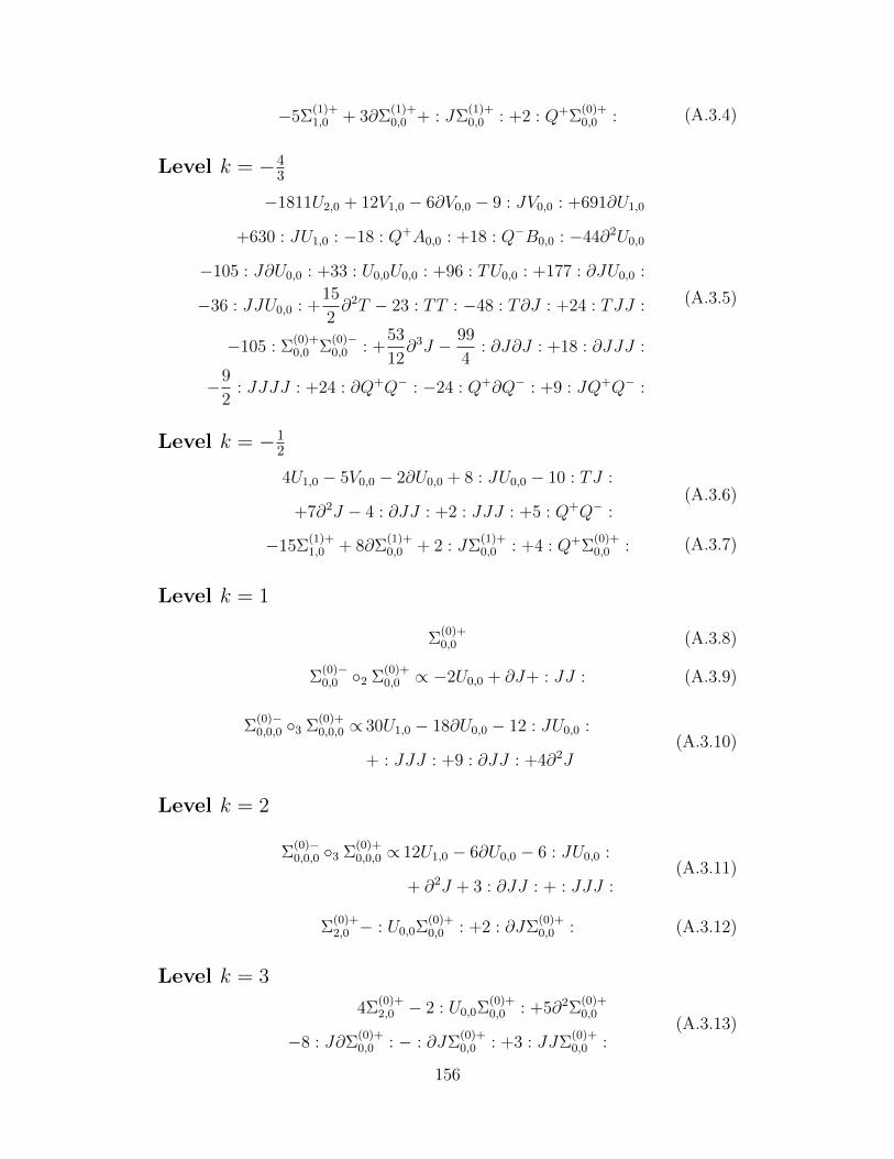
−5Σ(1)+1,0 + 3∂Σ

(1)+0,0 + : JΣ

(1)+0,0 : +2 : Q+Σ

(0)+0,0 : (A.3.4)

Level k = −43

−1811U2,0 + 12V1,0 − 6∂V0,0 − 9 : JV0,0 : +691∂U1,0

+630 : JU1,0 : −18 : Q+A0,0 : +18 : Q−B0,0 : −44∂2U0,0

−105 : J∂U0,0 : +33 : U0,0U0,0 : +96 : TU0,0 : +177 : ∂JU0,0 :

−36 : JJU0,0 : +15

2∂2T − 23 : TT : −48 : T∂J : +24 : TJJ :

−105 : Σ(0)+0,0 Σ

(0)−0,0 : +

53

12∂3J − 99

4: ∂J∂J : +18 : ∂JJJ :

−9

2: JJJJ : +24 : ∂Q+Q− : −24 : Q+∂Q− : +9 : JQ+Q− :

(A.3.5)

Level k = −12

4U1,0 − 5V0,0 − 2∂U0,0 + 8 : JU0,0 − 10 : TJ :

+7∂2J − 4 : ∂JJ : +2 : JJJ : +5 : Q+Q− :(A.3.6)

−15Σ(1)+1,0 + 8∂Σ

(1)+0,0 + 2 : JΣ

(1)+0,0 : +4 : Q+Σ

(0)+0,0 : (A.3.7)

Level k = 1

Σ(0)+0,0 (A.3.8)

Σ(0)−0,0 2 Σ

(0)+0,0 ∝ −2U0,0 + ∂J+ : JJ : (A.3.9)

Σ(0)−0,0,0 3 Σ

(0)+0,0,0 ∝ 30U1,0 − 18∂U0,0 − 12 : JU0,0 :

+ : JJJ : +9 : ∂JJ : +4∂2J(A.3.10)

Level k = 2

Σ(0)−0,0,0 3 Σ

(0)+0,0,0 ∝ 12U1,0 − 6∂U0,0 − 6 : JU0,0 :

+ ∂2J + 3 : ∂JJ : + : JJJ :(A.3.11)

Σ(0)+2,0 − : U0,0Σ

(0)+0,0 : +2 : ∂JΣ

(0)+0,0 : (A.3.12)

Level k = 3

4Σ(0)+2,0 − 2 : U0,0Σ

(0)+0,0 : +5∂2Σ

(0)+0,0

−8 : J∂Σ(0)+0,0 : − : ∂JΣ

(0)+0,0 : +3 : JJΣ

(0)+0,0 :

(A.3.13)

156

Appendix B

Characters of rectangularW-algebras at boundaryprincipal admissible level

Some additional notation is used in this appendix: The symbol ∝ is used

to indicate equality up to multiplication by aqbuc for a, b, c ∈ C where q =

exp(2πiτ) and u = exp(2πiz). For basis-dependent definitions of g of any type

we use the definitions as they are given in [GW09]. In particular, this allows

one to set

ι(x) =1

2

r−1∑j=0

s∑i=1

(s+ 1− 2i)ejs+i,js+i (B.0.1)

in all cases under consideration. Lastly, Id ∈Md×d(C) denotes the d-dimensional

identity matrix.

B.1 Type A

Using the standard basis εiNi=1 in h∗ which acts on the unit matrices via

εi(ej,j) = δi,j the set of positive roots of slN is given by ∆+ = δ1 ∪ δ2 where

δ1 =εj1n+i1 − εj2n+i2

∣∣1 ≤ i1, i2 ≤ n ∧ 0 ≤ j1 < j2 < m

δ2 =εjn+i1 − εjn+i2

∣∣1 ≤ i1 < i2 ≤ n ∧ 0 ≤ j < m.

Denote the intersection of the centralizer of ι(f) and the Cartan algebra of

slN by hι(f). One is quick to see that dim(hι(f)) = m− 1. Taking z ∈ hι(f) we

157

may write

z =m−1∑j=0

n∑i=1

cjejn+i,jn+i

or equivalently

z = diag(c0In, c1In, · · · , cm−1In)

under the condition that∑m−1

j=0 cj = 0. With this choice of notation it follows

that for α ∈ ∆+ as given above yields

α(z) = cj1 − cj2 and α(ι(x)) = −i1 + i2

It follows that ∆ 12

= ∅ and

∆0+ =

εj1n+i − εj2n+i

∣∣1 ≤ i ≤ n ∧ 0 ≤ j1 < j2 < m.

In order to compute the character of Wk(g, ι(f)) we use the formular given

in 6.1.3 and proceed by determining the products over subsets of the positive

roots. Let xj = exp(2πicj).∏α∈δ1

κ11(στ, α(z − τι(x))) ∝

∝∏

0≤j1<j2<m

∞∏r=1

n∏i1,i2=1

(1− xj2

xj1qσr−i1+i2

)(1− xj1

xj2qσ(r−1)+i1−i2

)=

∏0≤j1<j2<m

∞∏r=1

n∏i=0

(1− xj2

xj1qσr+n−i

)i(1− xj1

xj2qσ(r−1)−n+i

)i·n∏i=1

(1− xj2

xj1qσr−i

)n−i(1− xj1

xj2qσ(r−1)+i

)n−i

∝∏

0≤j1<j2<m

∞∏r=1

n+1∏i=1

(1− xj2

xj1qσr−i

)i−1(1− xj1

xj2qσ(r−1)+i

)i−1

·n∏i=1

(1− xj2

xj1qσr−i

)n−i(1− xj1

xj2qσ(r−1)+i

)n−i∝

∏0≤j1<j2<m

κ11(τ, cj1 − cj2)n−1κ11(στ, cj1 − cj2)

∏α∈δ2

κ11(στ, α(z − τι(x))) ∝

158

∝∏

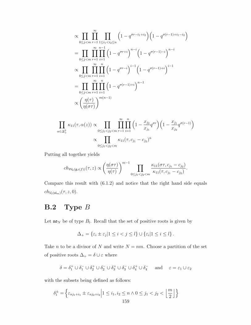
0≤j<m

∞∏r=1

∏1≤i1<i2≤n

(1− qσr−i1+i2

)(1− qσ(r−1)+i1−i2

)=∏

0≤j<m

∞∏r=1

n−1∏i=1

(1− qσr+i

)n−i(1− qσ(r−1)−i

)n−i∝∏

0≤j<m

∞∏r=1

n∏i=1

(1− qσr−i

)i−1(1− qσ(r−1)+i

)i−1

=∏

0≤j<m

∞∏r=1

n∏i=1

(1− qσ(r−1)+i

)n−1

∝(η(τ)

η(στ)

)m(n−1)

∏α∈∆0

+

κ11(τ, α(z)) ∝∏

0≤j1<j2<m

∞∏r=1

n∏i=1

(1− xj2

xj1qσr)(

1− xj1xj2

qσ(r−1))

∝∏

0≤j1<j2<m

κ11(τ, cj1 − cj2)n

Putting all together yields

chWk(g,ι(f))(τ, z) ∝(η(στ)

η(τ)

)m−1 ∏0≤j1<j2<m

κ11(στ, cj1 − cj2)

κ11(τ, cj1 − cj2).

Compare this result with (6.1.2) and notice that the right hand side equals

chV`(slm)(τ, z, 0).

B.2 Type B

Let soN be of type Bl. Recall that the set of positive roots is given by

∆+ = εi ± εj|1 ≤ i < j ≤ l ∪ εi|1 ≤ i ≤ l .

Take n to be a divisor of N and write N = nm. Choose a partition of the set

of positive roots ∆+ = δ ∪ ε where

δ = δ+1 ∪ δ−1 ∪ δ+

2 ∪ δ−2 ∪ δ+3 ∪ δ−3 ∪ δ+

4 ∪ δ−4 and ε = ε1 ∪ ε2

with the subsets being defined as follows:

δ±1 =εnj1+i1 ± εnj2+i2

∣∣∣1 ≤ i1, i2 ≤ n ∧ 0 ≤ j1 < j2 <⌊m

2

⌋159

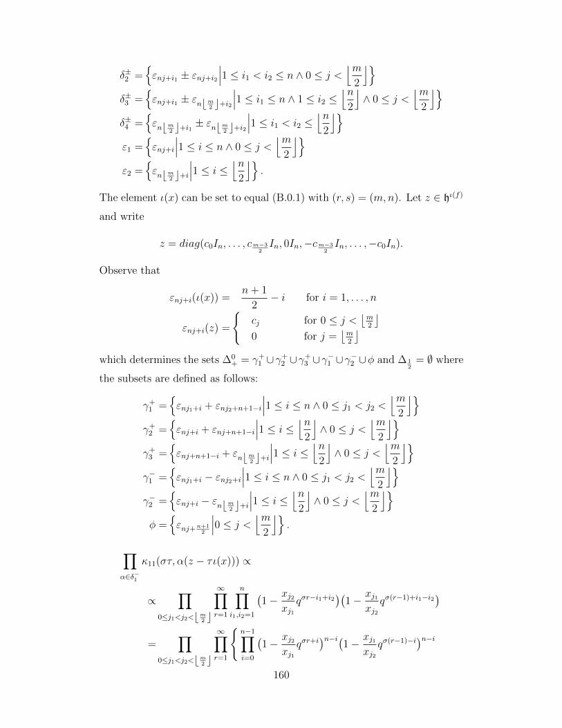
δ±2 =εnj+i1 ± εnj+i2

∣∣∣1 ≤ i1 < i2 ≤ n ∧ 0 ≤ j <⌊m

2

⌋δ±3 =

εnj+i1 ± εnbm2 c+i2

∣∣∣1 ≤ i1 ≤ n ∧ 1 ≤ i2 ≤⌊n

2

⌋∧ 0 ≤ j <

⌊m2

⌋δ±4 =

εnbm2 c+i1 ± εnbm2 c+i2

∣∣∣1 ≤ i1 < i2 ≤⌊n

2

⌋ε1 =

εnj+i

∣∣∣1 ≤ i ≤ n ∧ 0 ≤ j <⌊m

2

⌋ε2 =

εnbm2 c+i

∣∣∣1 ≤ i ≤⌊n

2

⌋.

The element ι(x) can be set to equal (B.0.1) with (r, s) = (m,n). Let z ∈ hι(f)

and write

z = diag(c0In, . . . , cm−32In, 0In,−cm−3

2In, . . . ,−c0In).

Observe that

εnj+i(ι(x)) =n+ 1

2− i for i = 1, . . . , n

εnj+i(z) =

cj for 0 ≤ j <

⌊m2

⌋0 for j =

⌊m2

⌋which determines the sets ∆0

+ = γ+1 ∪γ+

2 ∪γ+3 ∪γ−1 ∪γ−2 ∪φ and ∆ 1

2= ∅ where

the subsets are defined as follows:

γ+1 =

εnj1+i + εnj2+n+1−i

∣∣∣1 ≤ i ≤ n ∧ 0 ≤ j1 < j2 <⌊m

2

⌋γ+

2 =εnj+i + εnj+n+1−i

∣∣∣1 ≤ i ≤⌊n

2

⌋∧ 0 ≤ j <

⌊m2

⌋γ+

3 =εnj+n+1−i + εnbm2 c+i

∣∣∣1 ≤ i ≤⌊n

2

⌋∧ 0 ≤ j <

⌊m2

⌋γ−1 =

εnj1+i − εnj2+i

∣∣∣1 ≤ i ≤ n ∧ 0 ≤ j1 < j2 <⌊m

2

⌋γ−2 =

εnj+i − εnbm2 c+i

∣∣∣1 ≤ i ≤⌊n

2

⌋∧ 0 ≤ j <

⌊m2

⌋φ =

εnj+n+1

2

∣∣∣0 ≤ j <⌊m

2

⌋.

∏α∈δ−1

κ11(στ, α(z − τι(x))) ∝

∝∏

0≤j1<j2<bm2 c

∞∏r=1

n∏i1,i2=1

(1− xj2

xj1qσr−i1+i2

)(1− xj1

xj2qσ(r−1)+i1−i2

)

=∏

0≤j1<j2<bm2 c

∞∏r=1

n−1∏i=0

(1− xj2

xj1qσr+i

)n−i(1− xj1

xj2qσ(r−1)−i)n−i

160

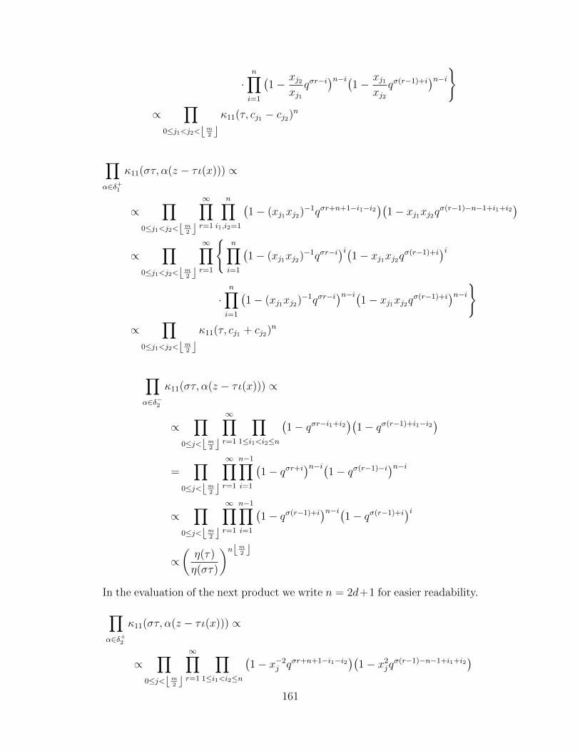
·n∏i=1

(1− xj2

xj1qσr−i

)n−i(1− xj1

xj2qσ(r−1)+i

)n−i∝

∏0≤j1<j2<bm2 c

κ11(τ, cj1 − cj2)n

∏α∈δ+

1

κ11(στ, α(z − τι(x))) ∝

∝∏

0≤j1<j2<bm2 c

∞∏r=1

n∏i1,i2=1

(1− (xj1xj2)−1qσr+n+1−i1−i2

)(1− xj1xj2qσ(r−1)−n−1+i1+i2

)

∝∏

0≤j1<j2<bm2 c

∞∏r=1

n∏i=1

(1− (xj1xj2)−1qσr−i

)i(1− xj1xj2qσ(r−1)+i

)i·n∏i=1

(1− (xj1xj2)−1qσr−i

)n−i(1− xj1xj2qσ(r−1)+i

)n−i∝

∏0≤j1<j2<bm2 c

κ11(τ, cj1 + cj2)n

∏α∈δ−2

κ11(στ, α(z − τι(x))) ∝

∝∏

0≤j<bm2 c

∞∏r=1

∏1≤i1<i2≤n

(1− qσr−i1+i2

)(1− qσ(r−1)+i1−i2

)

=∏

0≤j<bm2 c

∞∏r=1

n−1∏i=1

(1− qσr+i

)n−i(1− qσ(r−1)−i)n−i

∝∏

0≤j<bm2 c

∞∏r=1

n−1∏i=1

(1− qσ(r−1)+i

)n−i(1− qσ(r−1)+i

)i∝(η(τ)

η(στ)

)nbm2 cIn the evaluation of the next product we write n = 2d+1 for easier readability.∏α∈δ+

2

κ11(στ, α(z − τι(x))) ∝

∝∏

0≤j<bm2 c

∞∏r=1

∏1≤i1<i2≤n

(1− x−2

j qσr+n+1−i1−i2)(

1− x2jqσ(r−1)−n−1+i1+i2

)161

∝∏

0≤j<bm2 c

∞∏r=1

d∏i=1

(1− x−2

j qσr−2i)i(

1− x2jqσ(r−1)+2i

)i·(1− x−2

j qσr−(2i+1))i(

1− x2jqσ(r−1)+2i+1

)i·(1− x−2

j qσr−2d−2i)d+1−i(

1− x2jqσ(r−1)+2d+2i

)d+1−i

·(1− x−2

j qσr−2d−(2i+1))d−i(

1− x2jqσ(r−1)+2d+2i+1

)d−i∝

∏0≤j<bm2 c

κ11(τ, 2cj)bn2 c

∏α∈δ−3

κ11(στ, α(z − τι(x))) ∝

∝∏

0≤j<bm2 c

∞∏r=1

n∏i1=1

bn2 c∏i2

(1− x−1

j qσr−i1+i2)(

1− xjqσ(r−1)+i1−i2)

=∏

0≤j<bm2 c

∞∏r=1

bn2 c∏i2=1

(1− x−1

j qσr−n+i2)(

1− x−1j qσ(r−1)+n−i2

)

·bn2 c∏i1=1

((1− x−1

j qσr−i1+i2)(

1− x−1j qσ(r−1)+i1−i2

)·(1− x−1

j qσr−bn2 c−i1+i2

)(1− x−1

j qσ(r−1)+bn2 c+i1−i2))

=∏

0≤j<bm2 c

∞∏r=1

bn2 c∏i=1

((1− x−1

j qσ(r−1)+i)(

1− x−1j qσr−i

)·(1− x−1

j qσr+i)bn2 c−i(1− xjqσ(r−1)−i)bn2 c−i

·(1− x−1

j qσr−bn2 c+i)bn2 c−i(1− xjqσ(r−1)+bn2 c−i)bn2 c−i)

·bn2 c∏i=0

((1− x−1

j qσr−i)bn2 c−i(1− x−1

j qσ(r−1)+i)bn2 c−i

·(1− x−1

j qσr−bn2 c−i)bn2 c−i(1− x−1

j qσ(r−1)+bn2 c+i))bn2 c−i∝

∏0≤j<bm2 c

κ11(τ, cj)bn2 c

162

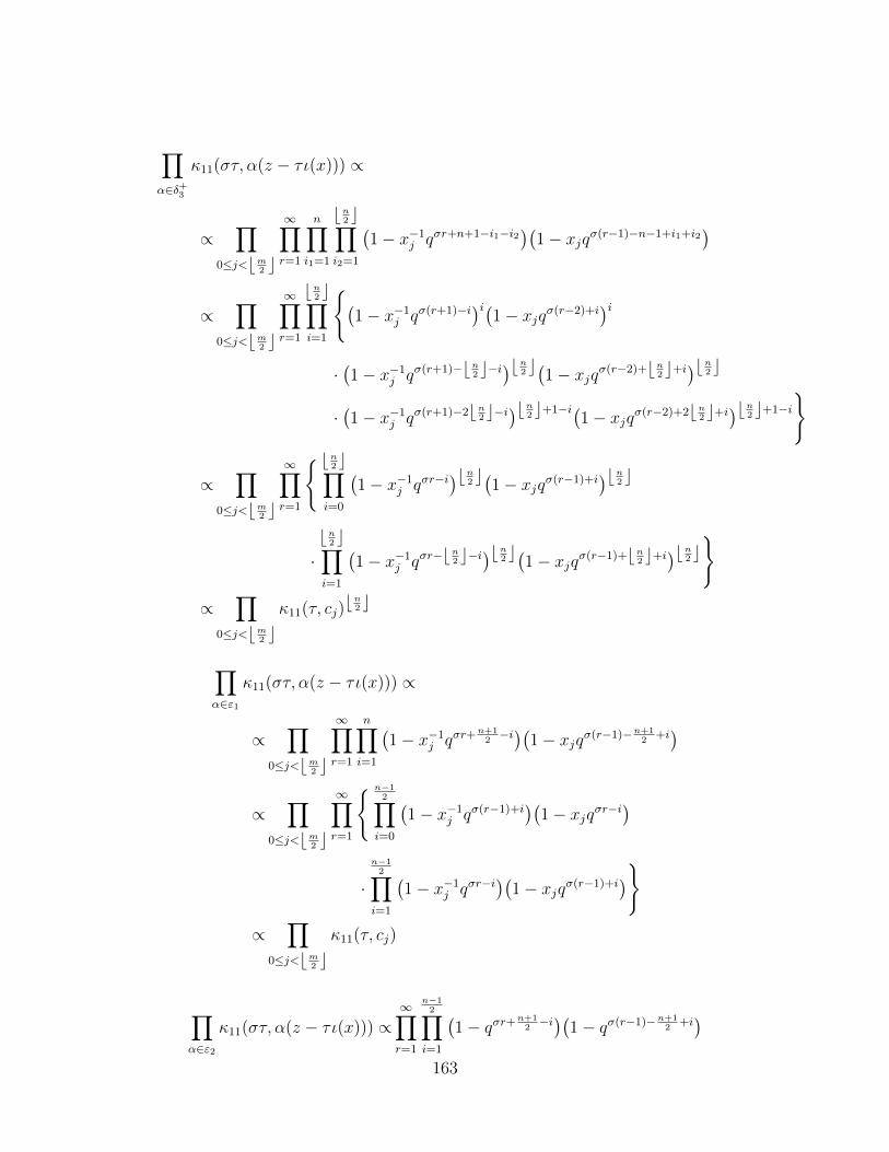
∏α∈δ+

3

κ11(στ, α(z − τι(x))) ∝

∝∏

0≤j<bm2 c

∞∏r=1

n∏i1=1

bn2 c∏i2=1

(1− x−1

j qσr+n+1−i1−i2)(

1− xjqσ(r−1)−n−1+i1+i2)

∝∏

0≤j<bm2 c

∞∏r=1

bn2 c∏i=1

(1− x−1

j qσ(r+1)−i)i(1− xjqσ(r−2)+i)i

·(1− x−1

j qσ(r+1)−bn2 c−i)bn2 c(1− xjqσ(r−2)+bn2 c+i)bn2 c·(1− x−1

j qσ(r+1)−2bn2 c−i)bn2 c+1−i(1− xjqσ(r−2)+2bn2 c+i)bn2 c+1−i

∝∏

0≤j<bm2 c

∞∏r=1

bn2 c∏i=0

(1− x−1

j qσr−i)bn2 c(1− xjqσ(r−1)+i

)bn2 c

·bn2 c∏i=1

(1− x−1

j qσr−bn2 c−i)bn2 c(1− xjqσ(r−1)+bn2 c+i)bn2 c

∝∏

0≤j<bm2 cκ11(τ, cj)

bn2 c

∏α∈ε1

κ11(στ, α(z − τι(x))) ∝

∝∏

0≤j<bm2 c

∞∏r=1

n∏i=1

(1− x−1

j qσr+n+1

2−i)(1− xjqσ(r−1)−n+1

2+i)

∝∏

0≤j<bm2 c

∞∏r=1

n−12∏i=0

(1− x−1

j qσ(r−1)+i)(

1− xjqσr−i)

·n−1

2∏i=1

(1− x−1

j qσr−i)(

1− xjqσ(r−1)+i)

∝∏

0≤j<bm2 cκ11(τ, cj)

∏α∈ε2

κ11(στ, α(z − τι(x))) ∝∞∏r=1

n−12∏i=1

(1− qσr+

n+12−i)(1− qσ(r−1)−n+1

2+i)

163

∝∞∏r=1

n−12∏i=1

(1− qσr−i

)(1− qσ(r−1)+i

)=∞∏r=1

n−12∏i=1

(1− qσ(r−1)+i

)∝ η(τ)

η(στ)

∏α∈γ+

1

κ11(τ, α(z)) ∝∏

0≤j1<j2<bm2 cκ11(τ, cj1 + cj2)n

∏α∈γ+

2

κ11(τ, α(z)) ∝∏

0≤j<bm2 cκ11(τ, 2cj)

bn2 c

∏α∈γ+

3

κ11(τ, α(z)) ∝∏

0≤j<bm2 cκ11(τ, cj)

bn2 c

∏α∈γ−1

κ11(τ, α(z)) ∝∏

0≤j1<j2<bm2 cκ11(τ, cj1 − cj2)n

∏α∈γ−2

κ11(τ, α(z)) ∝∏

0≤j<bm2 cκ11(τ, cj)

bn2 c

∏α∈φ

κ11(τ, α(z)) ∝∏

0≤j<bm2 cκ11(τ, cj)

∏α∈δ−4

κ11(στ, α(z − τι(x))) ∝∞∏r=1

∏1≤i1<i2≤bn2 c

(1− qσr−i1+i2

)(1− qσ(r−1)+i1−i2

)

∝∞∏r=1

bn2 c−1∏i=1

(1− qσr−i

)bn2 c−i(1− qσ(r−1)+i)bn2 c−i

For the evaluation of the remaining products two cases are distinguised: As-

suming that⌊n2

⌋= 2d or, equivalently, n = 4d+ 1 yields

∏α∈δ+

4

κ11(στ, α(z − τι(x))) ∝∞∏r=1

d∏i=1

(1− qσr−2i

)i(1− qσ(r−1)+2i

)i·

d∏i=2

(1− qσr−(2i−1)

)i−1(1− qσ(r−1)+2i−1

)i−1

·d−1∏i=1

(1− qσr−2d−(2i−1)

)d−i(1− qσ(r−1)+2d+2i−1

)d−i164

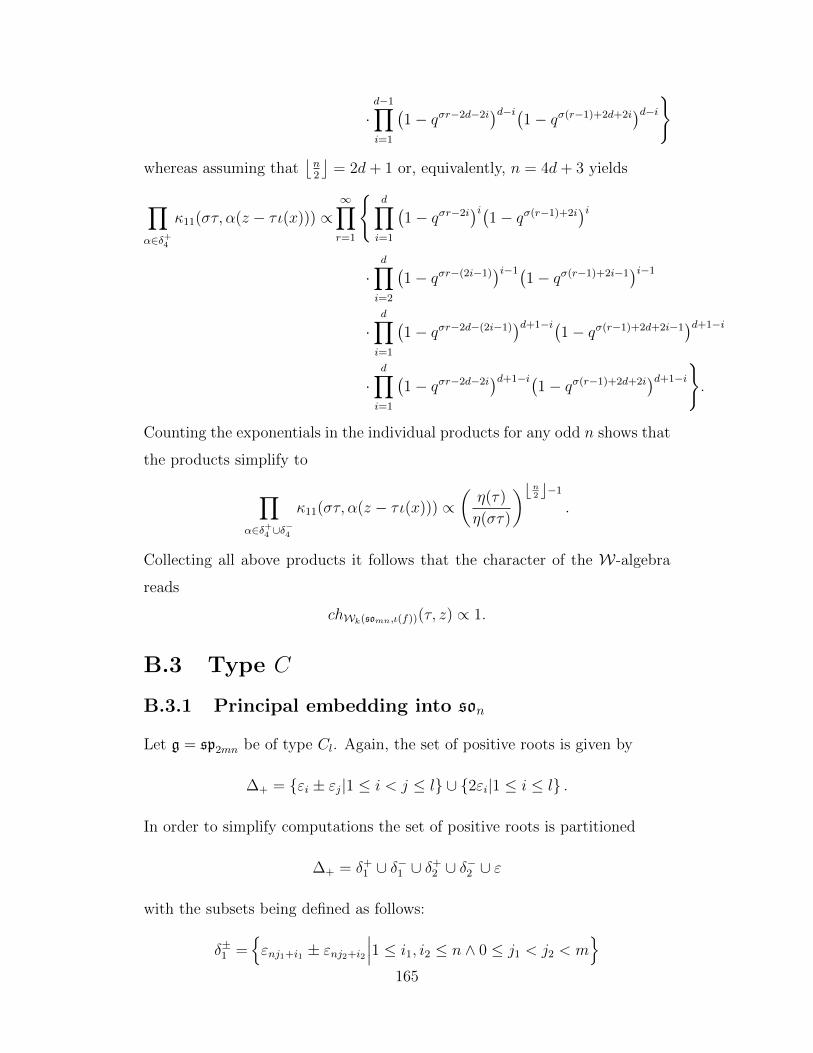
·d−1∏i=1

(1− qσr−2d−2i

)d−i(1− qσ(r−1)+2d+2i

)d−i

whereas assuming that⌊n2

⌋= 2d+ 1 or, equivalently, n = 4d+ 3 yields

∏α∈δ+

4

κ11(στ, α(z − τι(x))) ∝∞∏r=1

d∏i=1

(1− qσr−2i

)i(1− qσ(r−1)+2i

)i·

d∏i=2

(1− qσr−(2i−1)

)i−1(1− qσ(r−1)+2i−1

)i−1

·d∏i=1

(1− qσr−2d−(2i−1)

)d+1−i(1− qσ(r−1)+2d+2i−1

)d+1−i

·d∏i=1

(1− qσr−2d−2i

)d+1−i(1− qσ(r−1)+2d+2i

)d+1−i.

Counting the exponentials in the individual products for any odd n shows that

the products simplify to

∏α∈δ+

4 ∪δ−4

κ11(στ, α(z − τι(x))) ∝(η(τ)

η(στ)

)bn2 c−1

.

Collecting all above products it follows that the character of the W-algebra

reads

chWk(somn,ι(f))(τ, z) ∝ 1.

B.3 Type C

B.3.1 Principal embedding into son

Let g = sp2mn be of type Cl. Again, the set of positive roots is given by

∆+ = εi ± εj|1 ≤ i < j ≤ l ∪ 2εi|1 ≤ i ≤ l .

In order to simplify computations the set of positive roots is partitioned

∆+ = δ+1 ∪ δ−1 ∪ δ+

2 ∪ δ−2 ∪ ε

with the subsets being defined as follows:

δ±1 =εnj1+i1 ± εnj2+i2

∣∣∣1 ≤ i1, i2 ≤ n ∧ 0 ≤ j1 < j2 < m

165

δ±2 =εnj+i1 ± εnj+i2

∣∣∣1 ≤ i1 < i2 ≤ n ∧ 0 ≤ j < m

ε =

2εnj+i

∣∣∣1 ≤ i ≤ n ∧ 0 ≤ j < m

Taking n to be odd, the element ι(x) can be defined as in (B.0.1) with (r, s) =

(2m,n). Let z ∈ hι(f) and write

z = diag(c0In, . . . , cm−1In,−cm−1In, . . . ,−c0In).

Observe that

εnj+i(ι(x)) =n+ 1

2− i for i = 1, . . . , n

εnj+i(z) = cj for j = 1, . . . ,m− 1

which determines the sets ∆ 12

= ∅ and ∆0+ = γ+

1 ∪ γ+2 ∪ γ−1 ∪ φ where the

subsets are defined as follows:

γ+1 =

εnj1+i + εnj2+n+1−i

∣∣∣1 ≤ i ≤ n ∧ 0 ≤ j1 < j2 < m

γ+2 =

εnj+i + εnj+n+1−i

∣∣∣1 ≤ i ≤⌊n

2

⌋∧ 0 ≤ j < m

γ−1 =

εnj1+i − εnj2+i

∣∣∣1 ≤ i ≤ n ∧ 0 ≤ j1 < j2 < m

φ =

2εnj+n+12

∣∣∣0 ≤ j < m

In order to determine the character of Wk(g, ι(f)) we first consider all the

relevant products over the given subsets of the positive roots. Observe that

all but two of them have already been determined in B.2. Compared to B.2,

similar subsets of ∆+ and ∆0+ are suggestively given the same symbols with

the only difference being that m 7→ 2m. In particular, we have∏α∈∆+\ε κ11(στ, α(z − τι(x)))∏

α∈∆0+\φ

κ11(τ, α(z))∝(η(τ)

η(στ)

)nmTaking n = 2d+ 1 the remaining products are∏

α∈φ

κ11(τ, α(z)) ∝∏

0≤j<m

κ11(τ, 2cj)

and∏α∈ε

κ11(στ, α(z − τι(x))) ∝

166

∝∏

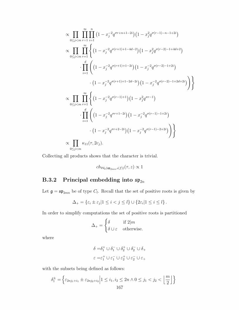
0≤j<m

∞∏r=1

n∏i=1

(1− x−2

j qσr+n+1−2i)(

1− x2jqσ(r−1)−n−1+2i

)∝∏

0≤j<m

∞∏r=1

(1− x−2

j qσ(r+1)+1−4d−2)(

1− x2jqσ(r−2)−1+4d+2

)·

d∏i=1

((1− x−2

j qσ(r+1)+1−2i)(

1− x−2j qσ(r−2)−1+2i

)·(1− x−2

j qσ(r+1)+1−2d−2i)(

1− x−2j qσ(r−2)−1+2d+2i

))

∝∏

0≤j<m

∞∏r=1

(1− x−2

j qσ(r−1)+1)(

1− x2jqσr−1

)·

d∏i=1

((1− x−2

j qσr+1−2i)(

1− x−2j qσ(r−1)−1+2i

)·(1− x−2

j qσr+2−2i)(

1− x−2j qσ(r−1)−2+2i

))∝∏

0≤j<m

κ11(τ, 2cj).

Collecting all products shows that the character is trivial.

chWk(sp2mn,ι(f))(τ, z) ∝ 1

B.3.2 Principal embedding into sp2n

Let g = sp2mn be of type Cl. Recall that the set of positive roots is given by

∆+ = εi ± εj|1 ≤ i < j ≤ l ∪ 2εi|1 ≤ i ≤ l .

In order to simplify computations the set of positive roots is partitioned

∆+ =

δ if 2|mδ ∪ ε otherwise.

where

δ =δ+1 ∪ δ−1 ∪ δ+

2 ∪ δ−2 ∪ δ+

ε =ε+1 ∪ ε−1 ∪ ε+

2 ∪ ε−2 ∪ ε+

with the subsets being defined as follows:

δ±1 =ε2nj1+i1 ± ε2nj2+i2

∣∣∣1 ≤ i1, i2 ≤ 2n ∧ 0 ≤ j1 < j2 <⌊m

2

⌋167

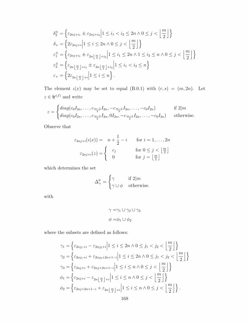
δ±2 =ε2nj+i1 ± ε2nj+i2

∣∣∣1 ≤ i1 < i2 ≤ 2n ∧ 0 ≤ j <⌊m

2

⌋δ+ =

2ε2nj+i

∣∣∣1 ≤ i ≤ 2n ∧ 0 ≤ j <⌊m

2

⌋ε±1 =

ε2nj+i1 ± ε2nbm2 c+i2

∣∣∣1 ≤ i1 ≤ 2n ∧ 1 ≤ i2 ≤ n ∧ 0 ≤ j <⌊m

2

⌋ε±2 =

ε2nbm2 c+i1 ± ε2nbm2 c+i2

∣∣∣1 ≤ i1 < i2 ≤ n

ε+ =

2ε2nbm2 c+i∣∣∣1 ≤ i ≤ n

.

The element ι(x) may be set to equal (B.0.1) with (r, s) = (m, 2n). Let

z ∈ hι(f) and write

z =

diag(c0I2n, . . . , cm−2

2I2n,−cm−2

2I2n, . . . ,−c0I2n) if 2|m

diag(c0I2n, . . . , cm−32I2n, 0I2n,−cm−3

2I2n, . . . ,−c0I2n) otherwise.

Observe that

ε2nj+i(ι(x)) = n+1

2− i for i = 1, . . . , 2n

ε2nj+i(z) =

cj for 0 ≤ j <

⌊m2

⌋0 for j =

⌊m2

⌋which determines the set

∆0+ =

γ if 2|mγ ∪ φ otherwise.

with

γ =γ1 ∪ γ2 ∪ γ3

φ =φ1 ∪ φ2

where the subsets are defined as follows:

γ1 =ε2nj1+i − ε2nj2+i

∣∣∣1 ≤ i ≤ 2n ∧ 0 ≤ j1 < j2 <⌊m

2

⌋γ2 =

ε2nj1+i + ε2nj2+2n+1−i

∣∣∣1 ≤ i ≤ 2n ∧ 0 ≤ j1 < j2 <⌊m

2

⌋γ3 =

ε2nj+i + ε2nj+2n+1−i

∣∣∣1 ≤ i ≤ n ∧ 0 ≤ j <⌊m

2

⌋φ1 =

ε2nj+i − ε2nbm2 c+i

∣∣∣1 ≤ i ≤ n ∧ 0 ≤ j <⌊m

2

⌋φ2 =

ε2nj+2n+1−i + ε2nbm2 c+i

∣∣∣1 ≤ i ≤ n ∧ 0 ≤ j <⌊m

2

⌋.

168

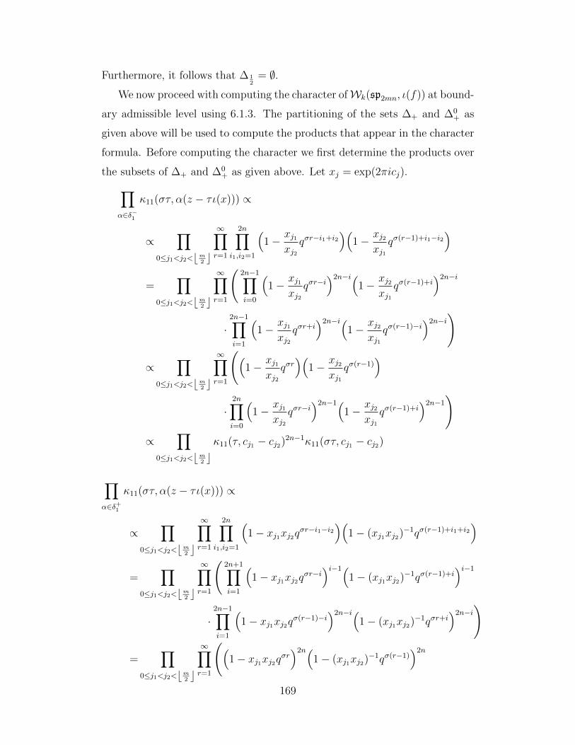
Furthermore, it follows that ∆ 12

= ∅.

We now proceed with computing the character ofWk(sp2mn, ι(f)) at bound-

ary admissible level using 6.1.3. The partitioning of the sets ∆+ and ∆0+ as

given above will be used to compute the products that appear in the character

formula. Before computing the character we first determine the products over

the subsets of ∆+ and ∆0+ as given above. Let xj = exp(2πicj).∏

α∈δ−1

κ11(στ, α(z − τι(x))) ∝

∝∏

0≤j1<j2<bm2 c

∞∏r=1

2n∏i1,i2=1

(1− xj1

xj2qσr−i1+i2

)(1− xj2

xj1qσ(r−1)+i1−i2

)

=∏

0≤j1<j2<bm2 c

∞∏r=1

(2n−1∏i=0

(1− xj1

xj2qσr−i

)2n−i(1− xj2

xj1qσ(r−1)+i

)2n−i

·2n−1∏i=1

(1− xj1

xj2qσr+i

)2n−i(1− xj2

xj1qσ(r−1)−i

)2n−i)

∝∏

0≤j1<j2<bm2 c

∞∏r=1

((1− xj1

xj2qσr)(

1− xj2xj1

qσ(r−1))

·2n∏i=0

(1− xj1

xj2qσr−i

)2n−1(1− xj2

xj1qσ(r−1)+i

)2n−1)

∝∏

0≤j1<j2<bm2 cκ11(τ, cj1 − cj2)2n−1κ11(στ, cj1 − cj2)

∏α∈δ+

1

κ11(στ, α(z − τι(x))) ∝

∝∏

0≤j1<j2<bm2 c

∞∏r=1

2n∏i1,i2=1

(1− xj1xj2qσr−i1−i2

)(1− (xj1xj2)−1qσ(r−1)+i1+i2

)

=∏

0≤j1<j2<bm2 c

∞∏r=1

(2n+1∏i=1

(1− xj1xj2qσr−i

)i−1(1− (xj1xj2)−1qσ(r−1)+i

)i−1

·2n−1∏i=1

(1− xj1xj2qσ(r−1)−i

)2n−i(1− (xj1xj2)−1qσr+i

)2n−i)

=∏

0≤j1<j2<bm2 c

∞∏r=1

((1− xj1xj2qσr

)2n(1− (xj1xj2)−1qσ(r−1)

)2n

169

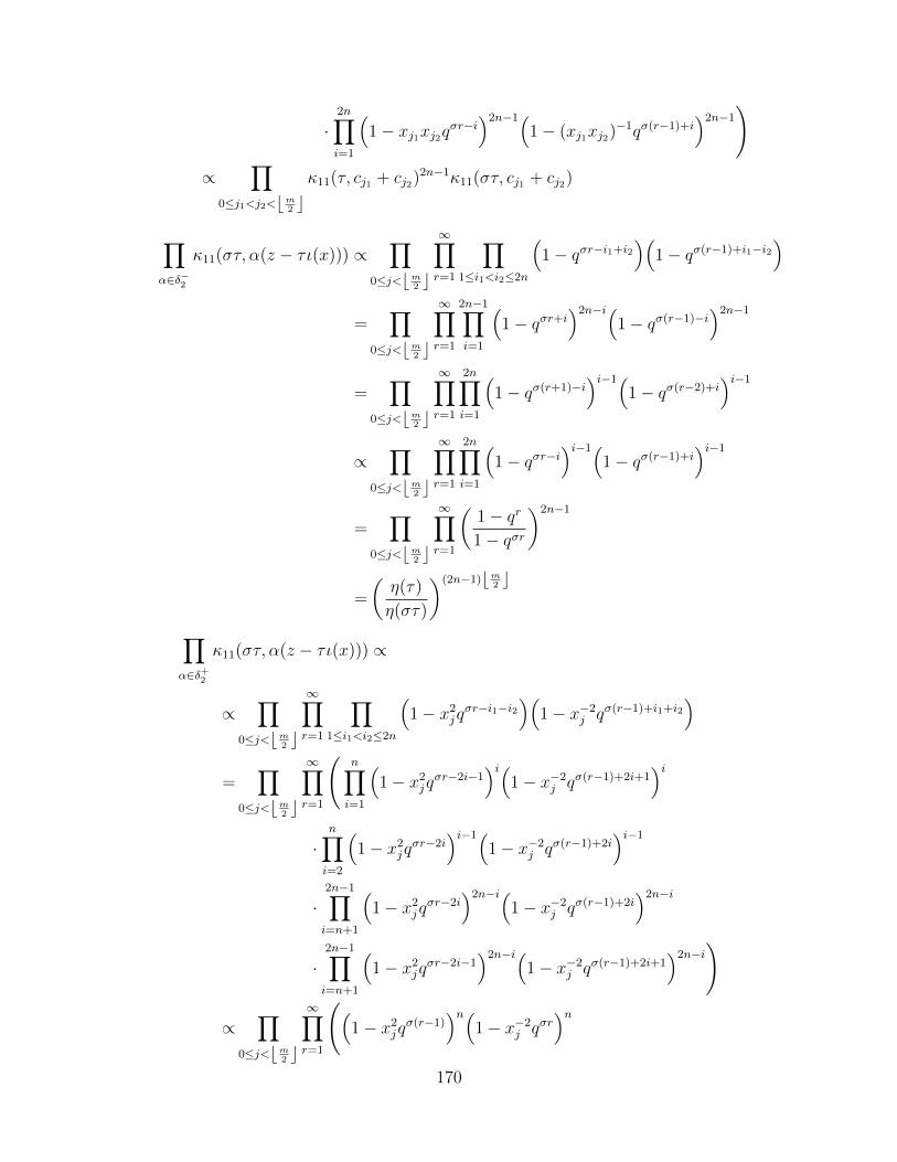
·2n∏i=1

(1− xj1xj2qσr−i

)2n−1(1− (xj1xj2)−1qσ(r−1)+i

)2n−1)

∝∏

0≤j1<j2<bm2 cκ11(τ, cj1 + cj2)2n−1κ11(στ, cj1 + cj2)

∏α∈δ−2

κ11(στ, α(z − τι(x))) ∝∏

0≤j<bm2 c

∞∏r=1

∏1≤i1<i2≤2n

(1− qσr−i1+i2

)(1− qσ(r−1)+i1−i2

)

=∏

0≤j<bm2 c

∞∏r=1

2n−1∏i=1

(1− qσr+i

)2n−i(1− qσ(r−1)−i

)2n−1

=∏

0≤j<bm2 c

∞∏r=1

2n∏i=1

(1− qσ(r+1)−i

)i−1(1− qσ(r−2)+i

)i−1

∝∏

0≤j<bm2 c

∞∏r=1

2n∏i=1

(1− qσr−i

)i−1(1− qσ(r−1)+i

)i−1

=∏

0≤j<bm2 c

∞∏r=1

(1− qr

1− qσr

)2n−1

=

(η(τ)

η(στ)

)(2n−1)bm2 c

∏α∈δ+

2

κ11(στ, α(z − τι(x))) ∝

∝∏

0≤j<bm2 c

∞∏r=1

∏1≤i1<i2≤2n

(1− x2

jqσr−i1−i2

)(1− x−2

j qσ(r−1)+i1+i2)

=∏

0≤j<bm2 c

∞∏r=1

(n∏i=1

(1− x2

jqσr−2i−1

)i(1− x−2

j qσ(r−1)+2i+1)i

·n∏i=2

(1− x2

jqσr−2i

)i−1(1− x−2

j qσ(r−1)+2i)i−1

·2n−1∏i=n+1

(1− x2

jqσr−2i

)2n−i(1− x−2

j qσ(r−1)+2i)2n−i

·2n−1∏i=n+1

(1− x2

jqσr−2i−1

)2n−i(1− x−2

j qσ(r−1)+2i+1)2n−i

)

∝∏

0≤j<bm2 c

∞∏r=1

((1− x2

jqσ(r−1)

)n(1− x−2

j qσr)n

170

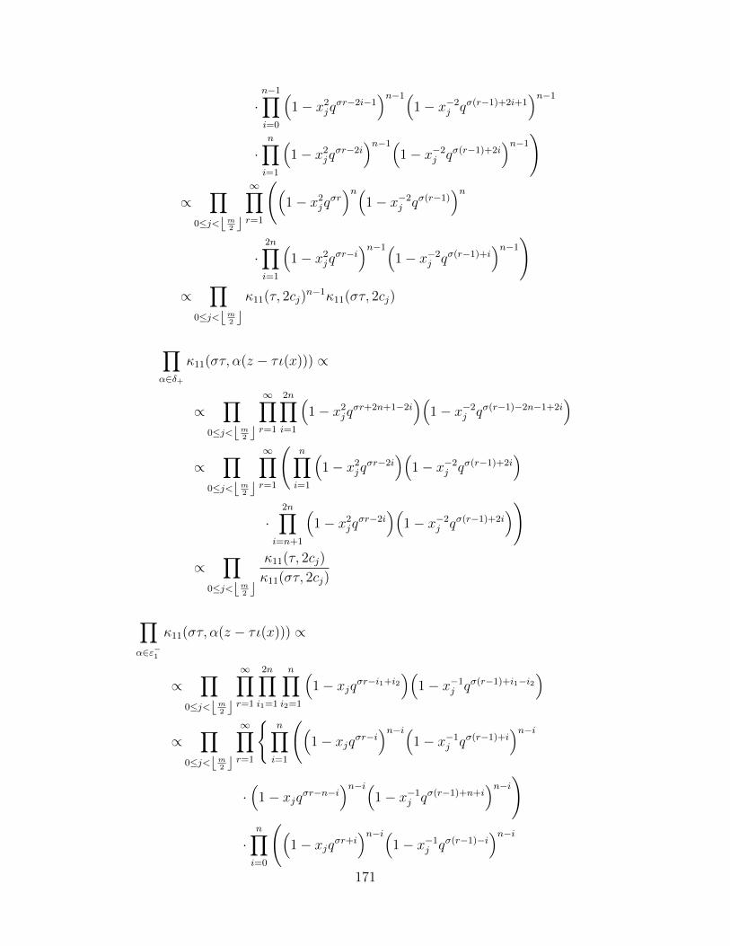
·n−1∏i=0

(1− x2

jqσr−2i−1

)n−1(1− x−2

j qσ(r−1)+2i+1)n−1

·n∏i=1

(1− x2

jqσr−2i

)n−1(1− x−2

j qσ(r−1)+2i)n−1

)

∝∏

0≤j<bm2 c

∞∏r=1

((1− x2

jqσr)n(

1− x−2j qσ(r−1)

)n

·2n∏i=1

(1− x2

jqσr−i

)n−1(1− x−2

j qσ(r−1)+i)n−1

)∝

∏0≤j<bm2 c

κ11(τ, 2cj)n−1κ11(στ, 2cj)

∏α∈δ+

κ11(στ, α(z − τι(x))) ∝

∝∏

0≤j<bm2 c

∞∏r=1

2n∏i=1

(1− x2

jqσr+2n+1−2i

)(1− x−2

j qσ(r−1)−2n−1+2i)

∝∏

0≤j<bm2 c

∞∏r=1

(n∏i=1

(1− x2

jqσr−2i

)(1− x−2

j qσ(r−1)+2i)

·2n∏

i=n+1

(1− x2

jqσr−2i

)(1− x−2

j qσ(r−1)+2i))

∝∏

0≤j<bm2 c

κ11(τ, 2cj)

κ11(στ, 2cj)

∏α∈ε−1

κ11(στ, α(z − τι(x))) ∝

∝∏

0≤j<bm2 c

∞∏r=1

2n∏i1=1

n∏i2=1

(1− xjqσr−i1+i2

)(1− x−1

j qσ(r−1)+i1−i2)

∝∏

0≤j<bm2 c

∞∏r=1

n∏i=1

((1− xjqσr−i

)n−i(1− x−1

j qσ(r−1)+i)n−i

·(

1− xjqσr−n−i)n−i(

1− x−1j qσ(r−1)+n+i

)n−i)

·n∏i=0

((1− xjqσr+i

)n−i(1− x−1

j qσ(r−1)−i)n−i

171

·(

1− xjqσr−n+i)n−i(

1− x−1j qσ(r−1)+n−i

)n−i)

∝∏

0≤j<bm2 c

∞∏r=1

n∏i=1

((1− xjqσr−i

)n−i(1− x−1

j qσ(r−1)+i)n−i

·(

1− xjqσr−n−i)n−i(

1− x−1j qσ(r−1)+n+i

)n−i)

·n+1∏i=1

(1− xjqσr−n−i

)i−1(1− x−1

j qσ(r−1)+n+i)i−1

·n∏i=0

(1− xjqσr−i

)i(1− x−1

j qσ(r−1)+i)i

∝∏

0≤j<bm2 c

(κ11(τ, cj)

n

n∏i=1

(1− xjqσr−n−i

)−1(1− x−1

j qσ(r−1)+n+i)−1)

∏α∈ε+1

κ11(στ, α(z − τι(x))) ∝

∝∏

0≤j<bm2 c

∞∏r=1

2n∏i1=1

n∏i2=1

(1− xjqσ(r+1)−i1−i2

)(1− x−1

j qσ(r−2)+i1+i2)

∝∏

0≤j<bm2 c

∞∏r=1

n∏i=1

(1− xjqσ(r+1)−i

)i−1(1− x−1

j qσ(r−2)+i)i−1

·(

1− xjqσ(r+1)−n−i)n(

1− x−1j qσ(r−2)+n+i

)n·(

1− xjqσ(r+1)−2n−i)n+1−i(

1− x−1j qσ(r−2)+2n+i

)n+1−i

∝∏

0≤j<bm2 c

∞∏r=1

(1− xjqσr

)n(1− x−1

j qσ(r−1))n

·n∏i=1

(1− xjqσr−i

)n−1(1− x−1

j qσ(r−1)+i)n−1

·(

1− xjqσr−n−i)n(

1− x−1j qσ(r−1)+n+i

)n

∝∏

0≤j<bm2 c

κ11(τ, cj)

n

n∏i=1

(1− xjqσr−i

)−1(1− x−1

j qσ(r−1)+i)−1

172

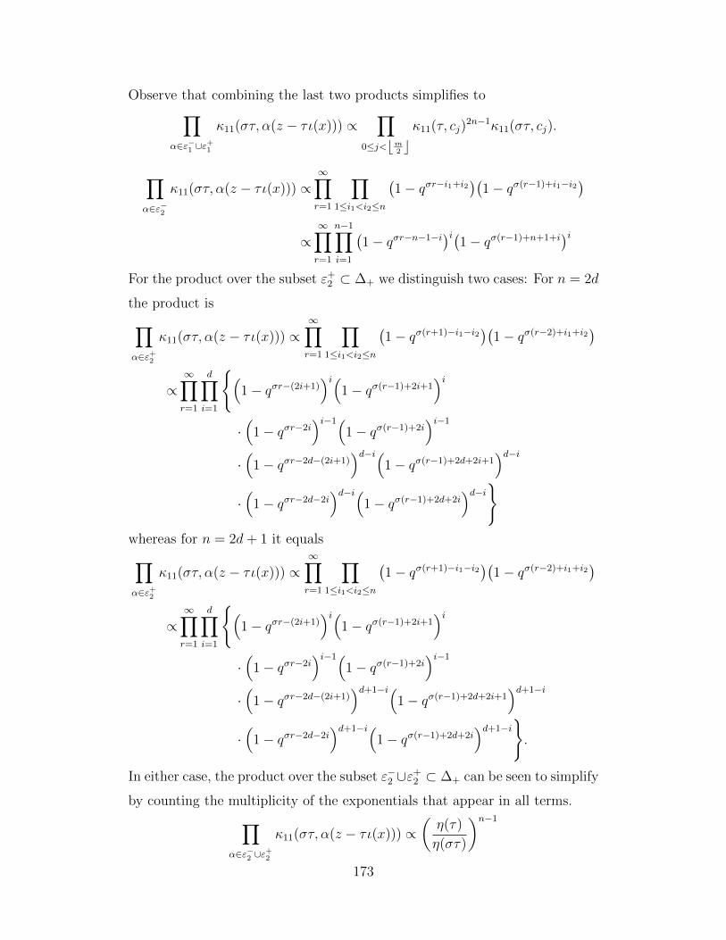
Observe that combining the last two products simplifies to∏α∈ε−1 ∪ε

+1

κ11(στ, α(z − τι(x))) ∝∏

0≤j<bm2 cκ11(τ, cj)

2n−1κ11(στ, cj).

∏α∈ε−2

κ11(στ, α(z − τι(x))) ∝∞∏r=1

∏1≤i1<i2≤n

(1− qσr−i1+i2

)(1− qσ(r−1)+i1−i2

)∝∞∏r=1

n−1∏i=1

(1− qσr−n−1−i)i(1− qσ(r−1)+n+1+i

)iFor the product over the subset ε+

2 ⊂ ∆+ we distinguish two cases: For n = 2d

the product is∏α∈ε+2

κ11(στ, α(z − τι(x))) ∝∞∏r=1

∏1≤i1<i2≤n

(1− qσ(r+1)−i1−i2

)(1− qσ(r−2)+i1+i2

)∝∞∏r=1

d∏i=1

(1− qσr−(2i+1)

)i(1− qσ(r−1)+2i+1

)i·(

1− qσr−2i)i−1(

1− qσ(r−1)+2i)i−1

·(

1− qσr−2d−(2i+1))d−i(

1− qσ(r−1)+2d+2i+1)d−i

·(

1− qσr−2d−2i)d−i(

1− qσ(r−1)+2d+2i)d−i

whereas for n = 2d+ 1 it equals∏α∈ε+2

κ11(στ, α(z − τι(x))) ∝∞∏r=1

∏1≤i1<i2≤n

(1− qσ(r+1)−i1−i2

)(1− qσ(r−2)+i1+i2

)∝∞∏r=1

d∏i=1

(1− qσr−(2i+1)

)i(1− qσ(r−1)+2i+1

)i·(

1− qσr−2i)i−1(

1− qσ(r−1)+2i)i−1

·(

1− qσr−2d−(2i+1))d+1−i(

1− qσ(r−1)+2d+2i+1)d+1−i

·(

1− qσr−2d−2i)d+1−i(

1− qσ(r−1)+2d+2i)d+1−i

.

In either case, the product over the subset ε−2 ∪ε+2 ⊂ ∆+ can be seen to simplify

by counting the multiplicity of the exponentials that appear in all terms.∏α∈ε−2 ∪ε

+2

κ11(στ, α(z − τι(x))) ∝(η(τ)

η(στ)

)n−1

173

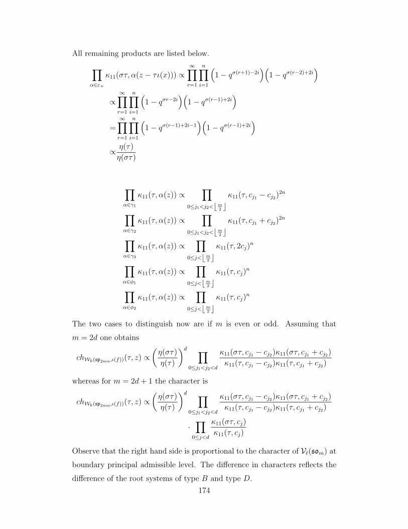
All remaining products are listed below.∏α∈ε+

κ11(στ, α(z − τι(x))) ∝∞∏r=1

n∏i=1

(1− qσ(r+1)−2i

)(1− qσ(r−2)+2i

)∝∞∏r=1

n∏i=1

(1− qσr−2i

)(1− qσ(r−1)+2i

)=∞∏r=1

n∏i=1

(1− qσ(r−1)+2i−1

)(1− qσ(r−1)+2i

)∝ η(τ)

η(στ)

∏α∈γ1

κ11(τ, α(z)) ∝∏

0≤j1<j2<bm2 cκ11(τ, cj1 − cj2)2n

∏α∈γ2

κ11(τ, α(z)) ∝∏

0≤j1<j2<bm2 cκ11(τ, cj1 + cj2)2n

∏α∈γ3

κ11(τ, α(z)) ∝∏

0≤j<bm2 cκ11(τ, 2cj)

n

∏α∈φ1

κ11(τ, α(z)) ∝∏

0≤j<bm2 cκ11(τ, cj)

n

∏α∈φ2

κ11(τ, α(z)) ∝∏

0≤j<bm2 cκ11(τ, cj)

n

The two cases to distinguish now are if m is even or odd. Assuming that

m = 2d one obtains

chWk(sp2mn,ι(f))(τ, z) ∝(η(στ)

η(τ)

)d ∏0≤j1<j2<d

κ11(στ, cj1 − cj2)κ11(στ, cj1 + cj2)

κ11(τ, cj1 − cj2)κ11(τ, cj1 + cj2)

whereas for m = 2d+ 1 the character is

chWk(sp2mn,ι(f))(τ, z) ∝(η(στ)

η(τ)

)d ∏0≤j1<j2<d

κ11(στ, cj1 − cj2)κ11(στ, cj1 + cj2)

κ11(τ, cj1 − cj2)κ11(τ, cj1 + cj2)

·∏

0≤j<d

κ11(στ, cj)

κ11(τ, cj)

Observe that the right hand side is proportional to the character of V`(som) at

boundary principal admissible level. The difference in characters reflects the

difference of the root systems of type B and type D.

174

B.4 Type D

Let soN be of type Dl. Recall that the set of positive roots is given by

∆+ = εi ± εj|1 ≤ i < j ≤ l .

In the case at hand we take N = 4nm and choose a partition of the set of

positive roots ∆+ = with the subsets being defined as follows:

δ±1 =ε2nj1+i1 ± ε2nj2+i2

∣∣∣1 ≤ i1, i2 ≤ 2n ∧ 0 ≤ j1 < j2 < m

δ±2 =ε2nj+i1 ± ε2nj+i2

∣∣∣1 ≤ i1 < i2 ≤ 2n ∧ 0 ≤ j < m

Set ι(x) as in (B.0.1) with (r, s) = (2m, 2n). Let z ∈ hι(f) and write

z = diag(c0I2n, . . . , cm−1I2n,−cm−1I2n, . . . ,−c0I2n).

Observe that

ε2nj+i(ι(x)) = n+1

2− i for i = 1, . . . , 2n

ε2nj+i(z) = cj for j = 0, . . . ,m− 1

which determines the sets ∆0+ = γ1 ∪ γ2 ∪ γ3 and ∆ 1

2= ∅ where the subsets

are defined as follows:

γ1 =ε2nj1+i − ε2nj2+i

∣∣∣1 ≤ i ≤ 2n ∧ 0 ≤ j1 < j2 < m

γ2 =ε2nj1+i + ε2nj2+2n+1−i

∣∣∣1 ≤ i ≤ 2n ∧ 0 ≤ j1 < j2 < m

γ3 =ε2nj+i + ε2nj+2n+1−i

∣∣∣1 ≤ i ≤ n ∧ 0 ≤ j < m

Before determining the character of the W-algebra we compute the products

over the given subsets of the positive roots. Observe that all of them have

been determined in B.3.2 where the relevant subsets are suggestively denoted

by the same symbols. The products are as follows:∏α∈δ+

1

κ11(στ, α(z − τι(x))) ∝∏

0≤j1<j2<m

κ11(τ, cj1 − cj2)2n−1κ(στ, cj1 − cj2)

∏α∈δ−1

κ11(στ, α(z − τι(x))) ∝∏

0≤j1<j2<m

κ11(τ, cj1 + cj2)2n−1κ(στ, cj1 + cj2)

175

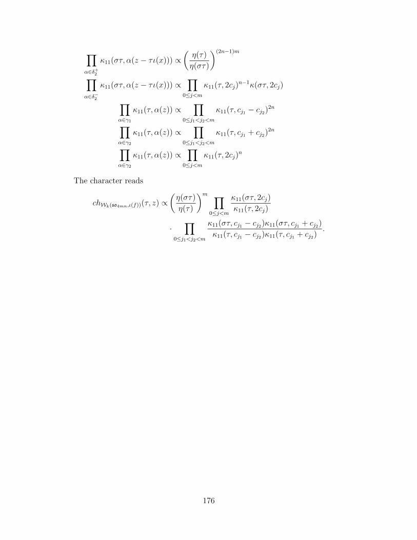
∏α∈δ+

2

κ11(στ, α(z − τι(x))) ∝(η(τ)

η(στ)

)(2n−1)m

∏α∈δ−2

κ11(στ, α(z − τι(x))) ∝∏

0≤j<m

κ11(τ, 2cj)n−1κ(στ, 2cj)

∏α∈γ1

κ11(τ, α(z)) ∝∏

0≤j1<j2<m

κ11(τ, cj1 − cj2)2n

∏α∈γ2

κ11(τ, α(z)) ∝∏

0≤j1<j2<m

κ11(τ, cj1 + cj2)2n

∏α∈γ2

κ11(τ, α(z)) ∝∏

0≤j<m

κ11(τ, 2cj)n

The character reads

chWk(so4mn,ι(f))(τ, z) ∝(η(στ)

η(τ)

)m ∏0≤j<m

κ11(στ, 2cj)

κ11(τ, 2cj)

·∏

0≤j1<j2<m

κ11(στ, cj1 − cj2)κ11(στ, cj1 + cj2)

κ11(τ, cj1 − cj2)κ11(τ, cj1 + cj2).

176