RADIO SCIENCE Journal of Research NBS/USNC-URSI Vol. 69D, No.7, July 1965

Aspects of the Terrestrial ELF Noise Spectrum When Near the Source or Its Antipode

L. G. Abraham, Jr. Applied Research Laboratory, Sylvania Electronic Systems, a Division of Sylvania Electric

Products, Inc., Waltham, Mass. 02154

(Received September 1, 1964; revised December 21, 1964)

Radiowave propagation in the extremely low frequency (ELF) range of 3 Hz to 3 kHz has been successfully treated in the past by a type of waveguide mode theory. This theory simplifies at large distances where only the zero order mode need be considered. It is shown in this paper that for frequencies in the band of 5 Hz to I kHz the zero order mode predominates at any distance in excess of roughly 500 km.

In a lower part of the ELF band (5 Hz to 100 Hz) more than one approximating form must be used. The commonly used asymptotic expansion applies only to a middle range of distances between source and receiver. When the receiver is within roughly one·sixth wavelength of either the source or its antipode then different approximations must be employed. These extensions of the theory are used in this paper to derive modifications of previous results for the terrestrial ELF noise power spectrum.

1. Introduction

The theory of extremely low frequency (ELF, 3 Hz to 3 kHz) radio wave propagation, developed by Schumann [1957] and Wait [1960a, b], predicts that the spherical cavity between the earth and the ionosphere will resonate at various frequencies for which the phase retardation in one circuit around the earth equals an integer number of complete cycles. This resonance phenomenon was observed experimentally in the natural noise background by Balser and Wagner [1960] over the "resonant" range of frequencies (5 to 50 Hz). These observations were fitted in some detail by Raemer [1961] who derived an expression for the power spectrum of the lightning flashes thought to be responsible. Improved explanations were given by Galejs [1961a, 1962] who had pre­viously developed a theory of ELF propagation (5 Hz to 1 kHz) for a more realistic model of ex· ponentially increasing conductivity with height in the isotropic ionosphere [Galejs, 1961b]. The earth's magnetic field was mostly ignored in these references and this paper will follow suit. The effect of such a static magnetic field has already been shown by Wait [1960b] to be largely negligible in the ELF band.

Some additions to the existing theory are needed in the resonance range when the noise source is close to the observer or his antipode. The work of both Raemer and Galejs was compared to observations taken by Balser and Wagner [1960, 1962] in the vicinity of Boston, Mass. The lightning stroke noise sources in these cases were mostly far distant from the receiver or its antipode. Hence, in this sense, the results of Raemer and Galejs are correct as they stand. The point of this paper is that they cannot be translated directly to measurements performed at sites close to the great tropical thunderstorm areas such as the Amazon or the Congo River basins (or their antipodes). All of the work presented here applies to the frequency range of 5 Hz to 1 kHz in agreement with the work of Galejs [1961b].

The waveguide mode theory of radio propagation is useful at ELF [Wait, 1960b] where the earth and the ionosphere form the lower and upper boundaries, respectively. The distance along the earth's surface is measured by the angle () subtended at its center. The individual modes in such a spherical system have a dependence on distance given by pv(n)(-COS (}), the Legendre func· tion of argument (-cos ()) and of complex degree v(n). In this paper the zero order mode (n = 0) is defined to be the mode of least attenuation in the ELF band. It is commonly stated that at large distances the zero order mode will predominate and the others can be ignored. This paper shows J

977

-

that the critical distance at which this first occurs is rO)lghly equal to 500 km; a value large com­pared to the height of the ionosphere and, to the first order, constant with frequency in the range of 5 Hz to 1 kHz_ The mode cutoff point around 3 kHz is not treated.

This last statement may seem to be at variance with previous ideas that one-sixth wavelength is a minimum distance. What Wait [1960b] has shown is that the normalized magnitude of the electric field varies in a linear manner with distance when the distance exceeds one-sixth wave­length and the frequency is in the range of 50 to 1600 Hz. However, the fact is that one-sixth wavelength also arises very naturally as the minimum distance needed to use a certain simplifying asymptotic expansion for Pv(O)( -cos 8). For frequencies below 100 Hz there is a range of distances running from 500 km out to one-sixth wavelength where thi~ first asymptotic form does not hold. But the zero order mode still predominates. Fortunately, a second expansion is available that does hold. Similarly, a third approximate form must be used when the radio wave source is within one-sixth wavelength of the observers' antipode. A second result of this paper is to present, under these latter two conditions, the necessary modifications to the formula of Galejs [1961a] for the terrestrial noise power spectrum.

2. Background Results In support of the main points of this paper, it is useful to set down some previously developed

approximations for the Legendre function Pv ( - cos 8) and the associated Legendre function of, first order P~( -cos 8). An approximation for the complex degree v(n) as a function of n( = 1! 2, ... )

is also given. These are results that are needed in various parts of this paper.

2.1. Approximate Forms for Pv (-cos 0) and p"l (-cos 0)

The various mathematical approximations quoted here can be found either in Bateman Manuscript Project [1953] or Magnus and Oberhettinger [1949] . They are grouped according to the relative position of the noise source and the receiver. Further approximations are shown that apply more particularly for the zero order mode since the complex degree v(O) is largely real [Galejs, 1961b].

The asymptotic expansions conventionally used in ELF propagation theory apply when the receiver is not too close to the source or its antipode. More explicitly,

. f(v+1) !2 Pv(- cos 8) = f(v + (3/2)) -y~ cos [(v + (1/2))(7T - 8) - (7T/4)]

1_ _ r(v+2) !2 _ PJ cos 8) - f(v+(3/2)) -y~ cos [(v + (l/2))(7T 8) + (7T/4)]

(1)

where r(z) is the gamma function of z.

Each of these is the first term of a trigonometric expansion. If the Sterling formula is used to approximate the gamma functions, the asymptotic expansions reduce to

P v( - cos 8) = V2/(v + (1/2))7T sin 8 cos [(v + (1/2))(7T - 8) - (7T/4)]

P~(-cos 8) = Y2(v+(l/2))/7T sin 8 cos [(v+(1/2))(7T-8)+ (7T/4)]

978

(2)

These last approximations are most appropriate in the case of the zero order mode where v(O)

is largely real. Wh~n the source is close to the antipode of the receiver an expansion of PvC- cos 8) for small

(7T - 8) is required. Probably the most rapidly convergent is a series, due to MacDonald, in terms of Bessel functions [Bateman Manuscript Project, 1953]. However, for the computations in this paper a better choice is based on the hypergeometric series de finition of the Legendre function,

PvC-cos 8) = 1

P~(- cos 8) = - v(v + 1) cos (8/2)

if I v I ( 7T - 8) ~ 1. (3)

Finally, when the sources are near the receiver itself a third approximation must be used to properly account for the singularity there. Materially differen t appearing express ions appl y, depending on whether the order is zero or positve [Bate man Manuscript Project, 1953] :

PvC- cos 8) = (sin (V7T)/7T) [2 log (sin (8/2» + C + 2iJ;(v + 1) + 7T cot (V7T) ]

P~(- cos 8) = - (sin (v7T)/7T)/si n (8/2)

iflvI8 ~ 1 and (4)

where C = Euler's consta nt = 0.5772 -

iJ;(z) = logarithmic deri vative of the Gamma function

., = d(log f(z»/dz = - C + 2: [(l/(n + 1» - (l /( n + z» ] .

n=O

These las t results complete the approximations needed to cover the e ntire range of polar a ngle.

2.2. Higher Order Roots of the Modal Equation

Wait [1960a] has already shown in the ELF band for a homogeneous ionospheric layer that only the zero order mode is freely propagating. The higher order modes (n ;;. 1) are below cutoff and thus heavily attenuated with distance. The same result can be obtained, using the zero order mode solution by Galejs [196lb], for a more realistic, exponentially increasing conductivity of the ionosphere. (The exponential model had been previously treated by Wait [1960a, b]. The solution, due to Galejs, represents an extension to that work.)

The complex degree v(n) is related to a mode factor 5n by the relation

where

k = free space, plane wave propagation constant a = radius of the earth.

(5)

The so·called modal equation is written in terms of 5n to satisfy boundary conditions at the earth and at the ionosphere. In the ELF band Galejs showed for the exponential ionosphere that 50 is largely real a nd close to unit magnitude, i.e., Re(5o) > 10 Im(50) and So = 1 for freque ncies from

979

-_. -- ---------------'

5 Hz to 1 kHz. He observed that this solution can be used to define an equivalent homogeneous ionosphere that will have an identical surface impedance Zj.

It can be said that 5 n is a function of Zi which, in turn, is related to So which is already known. Using the basic relations of Wait the end result is

5~ = 1- (7Tn/2kh)2[1 + VI + (2kh/7Tn)2(1-5~)]2 (6)

where h = height of the ionosphere above the earth. Detailed examination of numerical values for 50 [Galejs, I96Ib, 1962] shows that the square root can be expanded with little error. The paramo eter (2kh/7Tn)2(l-5&) has a maximum value of 0.1 at the upper frequency limit of 1 kHz.

After performing the expansion the higher order factors are approximated by

5; = - (7Tn/ kh)2 + (25~ - 1). (7)

Solving for the higher order complex degree (5) shows that to a close approximation

v(n) = - j(7Tan/h) + j(k2ah/27Tn)(25~ -1) = - j(7Tan/h). (8)

In this form, the first constant term on the right predominates (as shown) for frequencies from 5 Hz to 1 kHz. The higher order modes (n ;:3 1) have a complex degree that is largely imaginary. Thus, it follows that they are rapidly attenuated with distance.

3. Critical Distances The previous results are used in this section to help prove that the zero order mode begins to

predominate at distances in excess of 500 km. Also, the ranges of polar angle are specified where various approximate forms for this zero order mode apply.

3.1. Minimum Distance for Predominance of the Zero Order Mode

The vertical electric field at the earth's surface for a vertical current element at the surface is given by [Wait, I960a,b],

\

V(O) (v(O) + I)P ,,(0)( - cos 0)/2 sin V(O)7T 1 Er = (YJIds/2kha2)

+ f v(v + I)Pv( - cos O)/sin V7T n = l

where 0 = polar angle subtended by the sourCe and the observer at the center of the earth, YJ = characteristic impedance of free space = 120 7Til, k = free space, plane wave propagation constant,

Ids = moment of the vertical element, a = radius of the earth, h = height of the ionosphere above the earth.

(9)

Near the source all of the modes are required. At larger distances only the zero order mode has any significance since all the higher order modes are below cutoff.

The cutoff effect can be clearly seen by the following ar;proximation which applies at larger distances for the higher order mode term in the series for electric field.

Iv(v+ l)Pv( -cos O)/sin v7T1 = (7Tan/h)3/2V2/7T sin 0 exp (- (7Tan/h)O) (10)

980

for n ~ 1

(This result uses those of (2), (5), (7), and (8).) The parameter (7T an/h) has a minimum value of about 200 for an ionosphere of maximum height, h = 100 km. Hence, the exponential reduces the amplitude to negligible proportions.

The same type of approximation for the zero order mode term is

Iv(v+ 1)Pv( -cos 0)/2 sin v7T1 = v(v + 1) cos[ (v+0/2))(7T- 0)- (7T/4)]/(sin v7T)Y(2v+ 1)7T sin f)

(11)

for n=O

if IvlO P 1 and Ivl(7T - 0) P 1.

The degree v(O) has close to unit value. By comparison to the higher order mode (see (0)) the zero order mode predominates at any

large distance. Even its nulls are blunted by the slight propagation losses of the zero order mode.

As the distance (polar angle) is reduced, the logarithmic increase of P v(- cos 0) (see (4)) even­tually comes into play where all modes become important. In order for the zero order mode to predominate it is required that I v(n) I 0> > 1 be true for n ~ 1 so that the polar angle will stay well outside the range of logarithmic variation for high order modes.

The distance at which a particluar higher order mode can be neglected is given by

Oa > > a/ Iv(n) I = h/7Tn for n ~ 1 «8) used for I v I ). (2)

Obviously the first order mode is the limiting case. The minimum distance is simply required to be large compared to the height of the ionosphere. (As in ordinary waveguides the modes below cutoff are negligible a few guide widths downstream.) A distance of 500 km satisfies this last requirement under either day or night conditions. Note that this result is independent of frequency (to the first order) over the range of 5 Hz to 1 kHz.

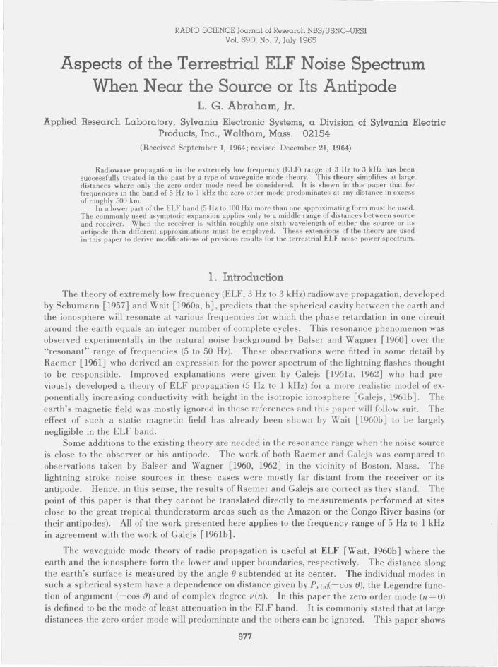
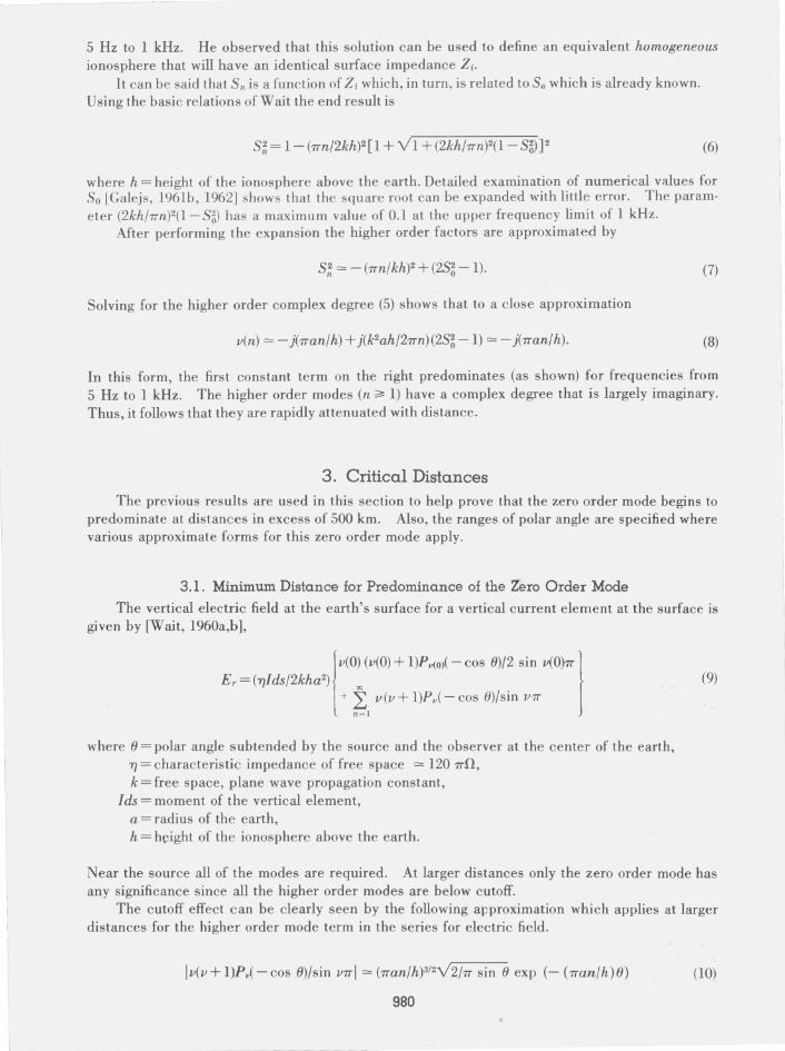
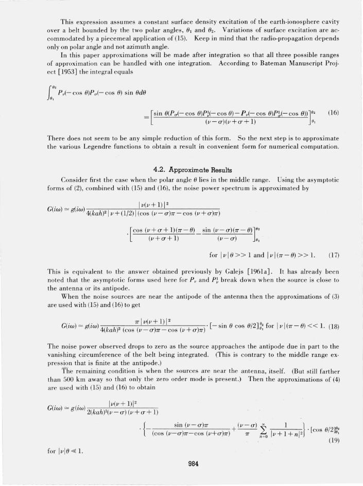
An example of the relative magnitude of the zero order and the first order modes is shown in figure 1. The first two terms in the series for the normalized vertical field, Er /(Tjlds/2kha2), are shown there. The zero order mode (n = 0) is shown in approximate form over the three ranges of distance that were outlined previously. The frequency of propagation is about 11 Hz, which

FIGURE 1. Magnitude of the zero order and first order mode terms from the series for normalized vertical elec· tric field versus distance from the source, using approxi­mations from the text.

981

-

IOO~--------------------------------.

n '" 1 FREQUENCY "" 11 Hz IONOSPHERIC HEIGHT -" 50 km SEE EQUArtON (9) FOR DETAILS.

0.01 '------'-----'----'----'-----'-----'-----"'--------'-----'-----' o 2 4 6 8 10 12 14 16 18 20

DISTANCE IN THOUSANDS OF KILOMETERS FROM THE SOURCE

~--------- - ----------

corresponds to a mInImUm in the natural resonance structure. The height of the ionosphere is 50 km as might be appropriate during the daytime. More will be said about the behavior of the zero order mode (with distance from the source) in later parts of this paper. But note that the first order mode has no important relative magnitude until the distance from the source is below 200 km. The selection of 500 km as the minimum distance for predominance of the zero order mode is very conservative.

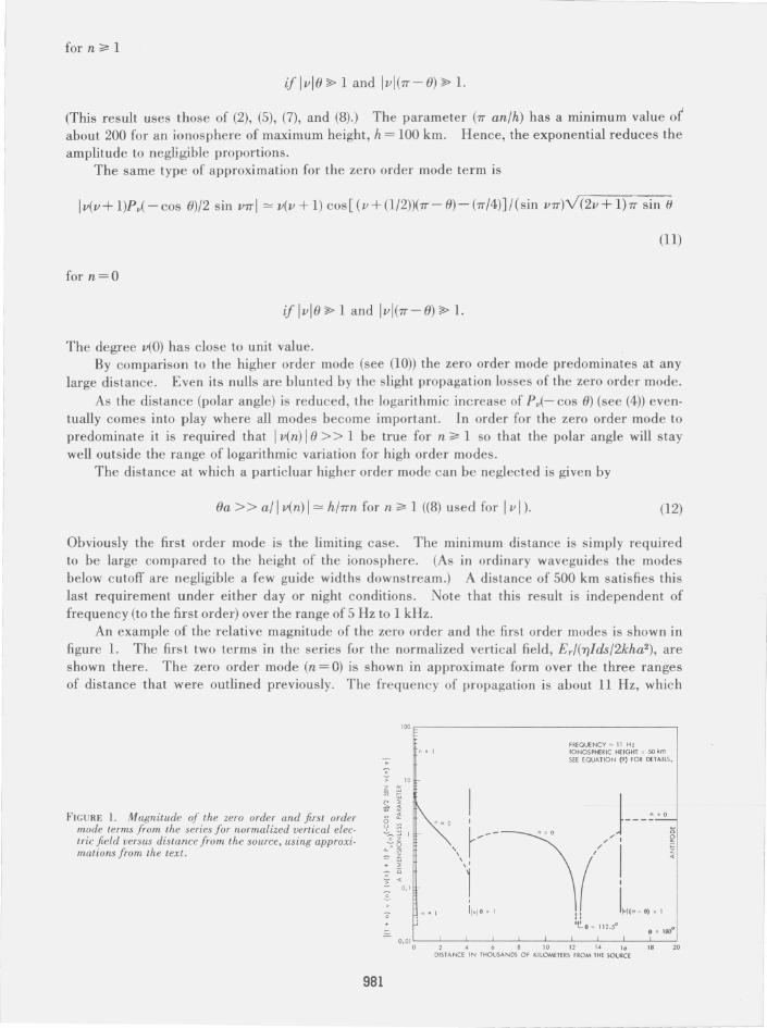
3.2. Bounding Distances Between the Three Approximations for the Zero Order Mode

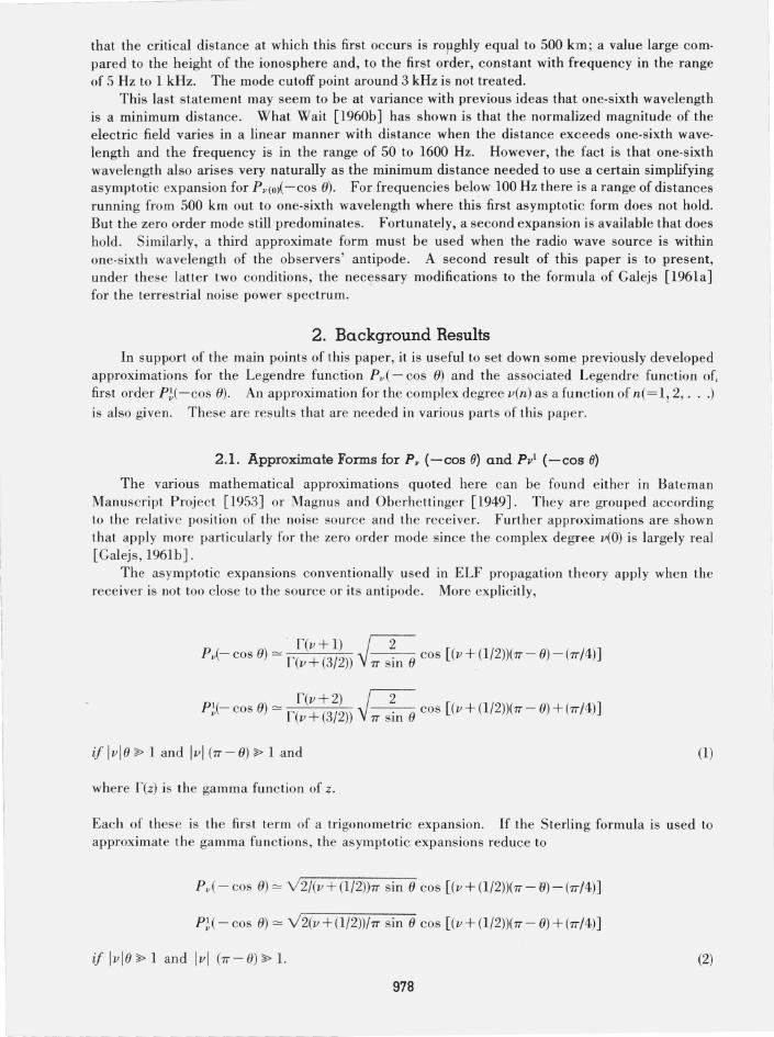
Figure 1 demonstrates the point that for low frequencies there is a range of source distances, from 500 km out to the place where III! 8 = 1, over which the normal asymptotic form for P v(-cos 8) does not apply. (The approximations of sec. 2 have been used in plotting the three ranges of dis· tance shown for the zero order mode.) The equivalent distance from the source that lies between these two ranges of approximation, is equal to

8a = a/ 111(0) 1= a/(- (1/2) + y'(kaSO)2 + (l/4)) (13)

where use has been made of (5). Figure 2 is a plot of this boundary distance from the source as a function of propagation frequency. If the distance is measured instead from the antipode of the source then the same curve is a second boundary between a second pair of distance ranges based on 1111 (7T - 0) = 1 (see fig. 1). Note that at higher frequencies this boundary is closely given by one-sixth wavelength.

It should be emphasized that the necessity for three different types of approximation to Pv(- cos 8) really only arises at the lower end of the ELF band in the normal propagation analysis. Figure 2 shows that the range of 5 Hz to 100 Hz is the frequency band affected. When the fre­quency exceeds 100 Hz the boundary distance is less than 500 km. The boundary distance is exceeded before the 500 km point is reached at which the zero order mode predominates_ Thus, it can be ignored in the normal propagation analysis that assumes solely zero order mode. Strictly speaking the special approximation for the area around the antipode of the source still applies . However, one might argue that the area involved is small enough for frequencies above 100 Hz that it could be ignored for all practical purposes.

Near the low end of the ELF band at 5 Hz the curve of figure 2 shows another phenomenon. The boundary distance between approximation regions has reached one-quarter of the distance around the earth. This boundary applies both around the source and its antipode. This means that the middle range of distances has disappeared, and the normal asymptotic expansion for p v(- cos 0) does not apply at any distance.

3.3. Higher Order Modes Within 500 km of the Antipode of the Source

One point of rigor remains in the treatment presented here. The antipode of the source is a natural focus at which the various mode amplitudes can be expected to increase. The zero

10

OL, ----~----~~--~IO----~------~--~ FREQUENCY IN Hz

982

FIGURE 2 . Distance /rom the source that separates two ranges 0/ approximation/or the zero order mode.

(Same curve is the bounda ry be tween another pair of ranges where di stance is from the a ntipode of the source.)

order mode should be checked to see that it predominates here also. Equation (10) shows the magnitude of the higher order modes would grow without bound except that that result does not apply within 500 km of the a ntipod e. (An argument s imilar to that of sec. 3.1, but using Iv(n)I(7T-O» > 1 instead of Iv(n) IO » 1, shows that (10) does not apply within 500 km of the antipode as well as 500 km of the source.) The correct approximation for high order mode terms within 500 km of the antipode is

I v(v + l)Pv(- cos 8)/sin V7T 1= 2(7Tan/h)2 exp (- (7Tan/h)7T)

for n;?; 1

if I v I (7T - 0) < < 1 (see sec. 2 for approximations). (14)

The 0 dependence has disappeared as the mode amplitude approaches a constant. The net conclusion is that even around the antipode the higher order mode terms (n ;?; 1) are negligible compared to the zero order mode. The exponential factor of (14) ins~res this fact just as in (10). The large differential attenuation between the higher order and zero order modes is not overcome by the focusin g experienced at the source antipode .

4. ELF Noise Spectrum Extensions

The integral for ELF noise power spectrum from a vertical stub antenna, due to li ghtning di s­c harge, has already been derived [Galejs, 1961a). The section evaluates thi s integral express ion when the sources are near the antenna or its antipode a nd the low-freq uency en d of th e ELF ba nd (5 to 100 Hz) is being considered. For the readers conve nie nce several parameters are redefined in thi s section. A s imilar discussion, appropriate to the vertical elec tri c fi eld inte nsi ty has been give n by Wait [1960b).

4 .1. Integral Expression

The s tarting point is the integral, jus t referred to, for received noise power spec trum of a short vertical antenna.

GC ) = g(.) 27TV(V + 1)a(a + 1) LW LW 16k2a2h2 s in va s in a7T (15)

i 82 P v( - cos O)P (J"( - cos 0) sin OdO 8 1

where g(iw) = quantity proportional to the squared dipole moment of the lightning disc harges per unit area (assumed independent of position), and

w = radian frequency, k = free space, plane wave propagation factor, a = radius of the earth, h = height of the lower edge of the ionosphere, 0= polar angle at the center of the earth measured from noise source to receiving antenna,

So = zero ord er root of the modal equation, a complex number that is largely real and close to unity.

v(v+ 1) = (kaSo)2, a = complex conjugate of v,

P iz) = Legendre function of z with degree v.

767- 936 0 - 65- 6 983 _J

This expression assumes a constant surface density excitation of the earth-ionosphere cavity over a belt bounded by the two polar angles, e J and ez. Variations of surface excitation are ac­commodated by a piecemeal application of (15). Keep in mind that the radio-propagation depends only on polar angle and not azimuth angle.

In this paper approximations will be made after integration so that all three possible ranges of approximation can be handled with one integration. According to Bateman Manuscript Proj· ect [1953] the integral equals

i 02 P i- cos e)p (J"(- cos e) sin ede

0,

= [sin e(p (J"(- cos e)p!(- cos e) - p v(- cos e)p~(- cos e))]02 (v-a)(v+a+l) 0,

(16)

There does not seem to be any simple reduction of this form. So the next step is to approximate the various Legendre functions to obtain a result in convenient form for numerical computation.

4.2. Approximate Results

Consider first the case when the polar angle e lies in the middle range. Using the asymptotic forms of (2), combined with (15) and (16), the noise power spectrum is approximated by

G(iw) = g(iw) 1 v(v + 1) IZ 4(kah)ZI v + (1/2) 1 (cos (v - a)7T - cos (v + a)7T)

. [cos (v + a + 1)(7T - e) (v+a+l)

sin (v-a)(7T- 8)]02 (v - a) 0,

forlvle»landlvl(7T-e»>l. (17)

This is equivalent to the answer obtained previously by Galejs [1961a] . It has already been noted that the asymptotic forms used here for p" and P! break down when the source is close to the antenna or its antipode.

When the noise sources are near the antipode of the antenna then the approximations of (3) are used with (15) and (16) to get

G(iw)=g(iw)4(k h)Z( ~lv(v~l)IZ (+) )'[-sinecos8/2U2forlvl(7T-e)«1. (18) a cos v - a 7T - cos V a 7T '

The noise power observed drops to zero as the source approaches the antipode due in part to the vanishing circumference of the belt being integrated. (This is contrary to the middle range ex­pression that is finite at the antipode.)

The remaining condition is when the sources are near the antenna, itself. (But still farther than 500 km away so that o~ly the zero order mode is present.) Then the approximations of (4) are used with (15) and (16) to obtain

. . Iv(v+l)I Z G(LW) = g(LW) 2(kah)Z(v - a) (v + a + 1)

{ sin (v - a)7T + (v - a) oc I} " . - --- '" . [cos 8/2]V2

(cos (v-a)7T-cos (v+a)7T) 7T ~o Iv+ 1 + nl2 0,

. (19)

984

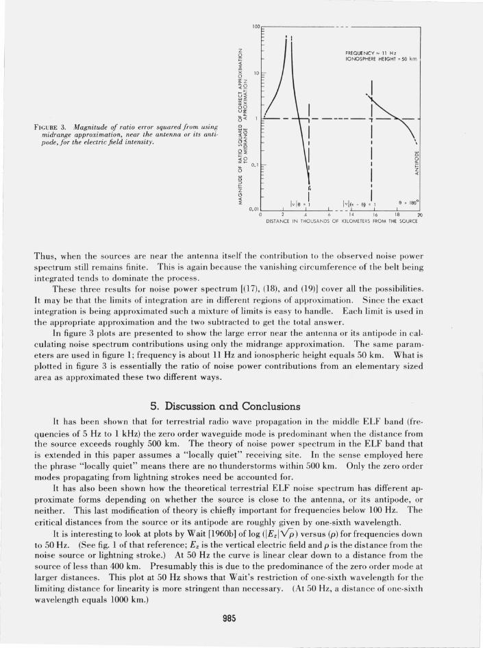
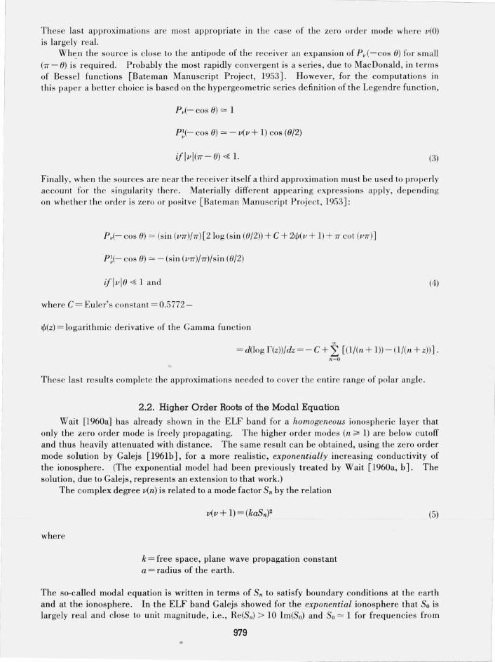
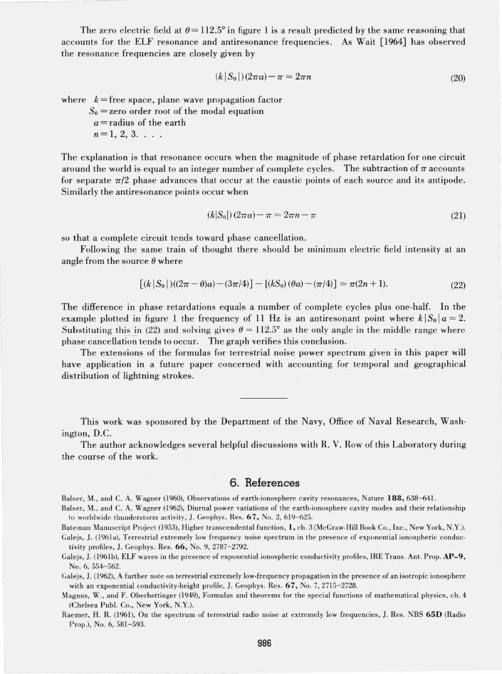
FIGURE 3. Magnitude of ratio error squared from using midrange approximation, near the antenna or its anti­pode, for the electric field intensity.

Cl

2 z " ~

FREQUENCY ~ II Hz IONOSPHERE HE IGHT = 50 km

.1 I ~ 1------1--\ -I I \

1 I I

I (. i Ivls= \ H(,-S)=I

0. 01 0'----:---.. '----6'- 14 16 IS ;>()

DISTANCE IN THOUSANDS OF KILOMETE RS FROM THE SOURCE

Thus, whe n the sources are near the antenna itself the contribution to the observed noise power spectrum still remains finite. This is again because the vani shing ci rc umference of the belt being integrated te nd s to dominate the process.

These three res ults for noise power spectrum [(17), (18), and (19)] cover all the possibilities . It may be that the limits of integration are in differe nt regions of approximation. Since the exac t integration is being approximated such a mixture oflimits is easy to handle. Each limit is used in th e appropriate approximation and the two subtracted to get the total answer.

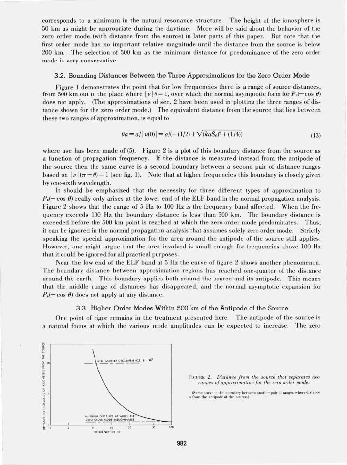
In figure 3 plots are presented to show the large error near the antenna or its antipode in cal­culating noise spectrum contributions using only the midrange approximation. The same param­eters are used in figure 1; frequency is about 11 Hz and ionospheric height equals 50 km . Whatis plotted in figure 3 is essentially the ratio of noise power contributions from an elementary sized area as approximated these two different ways.

5. Discussion and Conclusions It has been shown that for terrestrial radio wave propagation in the middle ELF band (fre­

quencies of 5 Hz to 1 kHz) the zero order waveguide mode is predominant whe n the distance from the source exceeds roughly 500 km. The theory of noise power spectrum in the ELF band that is extended in this paper assumes a "locally quiet" receiving site. In the sense e mployed here the phrase "locally quiet" means there are no thunderstorms within 500 km. Only the zero order modes propagating from lightning strokes need be accounted for.

It has also been shown how the theoretical terrestrial ELF noise spectrum has different ap­proximate forms depending on whether the source is close to the antenna, or its antipode, or neither. This last !podification of theory is chiefly important for frequencies below 100 Hz. The critical distances from the source or its antipode are roughly given by one-sixth wavelength.

It is interesting to look at plots by Wait [1960b] of log (IEzIVp) versus (p) for frequencies down to 50 Hz. (See fig. 1 of that reference; Ez is the vertical electric field and p is the distance from the noise source or lightning stroke.) At 50 Hz the curve is linear clear down to a distance from the source of less than 400 km. Presumably this is due to the predominance of the zero order mode at larger distances. This plot at 50 Hz shows that Wait's restriction of one-sixth wavelength for th e limiting distance for linearity is more stringent than necessary. (At 50 Hz, a di s tance of one·sixth wavelength equals 1000 km.)

985

- - - - - ------

The zero electric field at () = 112.5° in figure 1 is a re!1ult predicted by the same reasoning that accounts for the ELF resonance and antiresonance frequencies. As Wait [1964] has observed the resonance frequencies are closely given by

(k I So I )(27Ta) -7T = 27Tn

where k = free space, plane wave propagation factor So = zero order root of the modal equation a = radius of the earth n=l, 2, 3 ....

(20)

The explanation is that resonance occurs when the magnitude of phase retardation for one circuit around the world is equal to an integer number of complete cycles. The subtraction of 7T accounts for separate 7T/2 phase advances that occur at the caustic points of each source and its antipode. Similarly the antiresonance points occur when

(kISol) (27Ta) - 7T = 27Tn - 7T (21)

so that a complete circuit tends toward phase cancellation. Following the same train of thought there should be minimum electric field intensity at an

angle from the source () where

[(k 150 I )((27T- (})a)-(37T/4)] - [(kSo) ((}a) -(7T/4)] = 7T(2n+ 1). (22)

The difference in phase retardations equals a number of complete cycles plus one-half. In the example plotted in figure 1 the frequency of 11 Hz is an antiresonant point where k I So I a = 2. Substituting th~~_in (22) and solving gives (J = 112.5° as the only angle in the middle range where phase cancellation tends to occur. The graph verifies this conclusion.

The extensions of the formulas for terrestrial noise power spectrum given in this paper will have application in a future paper concerned with accounting for temporal and geographical distribution of lightning strokes.

This work was sponsored by the Department of the Navy, Office of Naval Research, Wash­ington, D.C.

The author acknowledges several helpful discussions with R. V. Row of this Laboratory during the course of the work.

6. References Balser, M., and C. A. Wagner (1960), Observations of e arth-ionosphere cavity resonances, Nature 188,638- 641. Balser, M., and C. A. Wagner (1962), Diurnal power variations of the earth-ionosphere cavity modes and their relationship

to world wide thunderstorm activity, J. Geophys. Res . 67, No. 2, 61 9-625. Bate man Manuscript Project (1953), Higher transcendental function, I, ch. 3 (McGraw-Hill Book Co., Inc., New York, N.Y.). Galejs, J. (l961a), Terrestrial extremely low frequency noise spectrum in the presence of exponential ionospheric conduc­

tivity profiles, J. Geophys . Res. 66, No. 9, 2787-2792. Galejs, J. (1961b), ELF waves in the presence of expone ntial ionospheric conductivity profiles, IRE Trans. Ant. Prop. AP-9,

No.6, 554-562. Galejs,1. (1962), A further note on terrestrial extremely low-frequency propagation in the presence of an isotropic ionosphere

with an exponential condu ctivity-height profile, J. Geophys. Res . 67, No .7, 2715-2728. Magnus, W., and F. Oberhettinger (1949), Formulas and theorems for the special functions of mathematical physics, ch. 4

(Chelsea Pub!. Co. , New York, N.Y.). Raemer, H. R. (1961), On the spectrum of terres trial radio noise at extremely low frequencies, 1. Res. NBS 65D (Radio

P rop.), No. 6, 581- 593.

986

- ------ ------

Schumann, W. O. (1957), Elektrische Eigenschwingungen des Hohlrau mes Erde·Luft-Ionosphere, Z. angew, Phys . 9, 373-378.

Wait, 1. R. (1960a), Terres trial propagation of very.low frequen cy radio waves, J. Res. NBS 64D (Radio Prop.), No.2, 153-204.

Wait, 1. R. (l960b), Mode theory and the propagation of ELF radio waves , J. Res. NBS 64D (Radio Prop.), No.4, 387-404. Wait, 1. R. (1964), On the theory of Schumann resonances in the earth-ionosphere cavity, Can. J. Phys. 42, No.4, 575-582.

(Paper 69D7-532)

987

~- - - ---~--------