ASME TurboExpo2014 FinalSubmission

1 Copyright © 2014 by ASME

Proceedings of ASME Turbo Expo 2014: Turbine Technical Conference and Exposition GT2014

June 16-20, 2014, Düsseldorf, Germany

GT2014-26048 GPGPU BASED AEROACOUSTIC OPTIMIZATION OF A CONTRA-ROTATING FAN

Michael Stadler Ninsight

Graz, Austria

Michael B. Schmitz ebm-papst St. Georgen St. Georgen, Germany

Wolfgang Laufer ebm-papst St. Georgen St. Georgen, Germany

ABSTRACT Contra-rotating fans have several advantages over single

stage axial fans. If they are well designed, the exit flow field is almost irrotational. This helps to increase the aerodynamic efficiency by up to 16%, when compared to single stage fans. However, since the second stage interacts with the flow disturbances from the first stage, the associated noise generation is a disadvantage. This may be remedied by carefully tuning the design.

The optimization of a contra-rotating fan involves a large set of design parameters. These include the geometrical parameters of the fan blades, the winglets, the guide vane as well as the hub diameter. We demonstrate an evolutionary algorithm which helps to automate the optimization process. It is controlled by two objective functions: (1) aerodynamic efficiency and (2) the emitted tonal noise.

For the evaluation of the sound pressure, we implemented a new lattice-Boltzmann solver. Due to its algorithmic structure, this is ideally suited for massive parallelization. To leverage this potential, it is designed to run on general-purpose graphics processing units (GPGPUs). To further accelerate the optimization, it is supported by a meta-model based on a radial-basis function network.

We demonstrate the method for a small contra-rotating fan. Our numerical results are compared with physical tests. The new algorithmic arrangement has shown to drastically cut development costs and time.

INTRODUCTION Contra-rotating fans are used for high-performance

applications. They are able to deliver more airflow and higher static pressure than two conventional fans of the same size in serial configuration. However, their most important disadvantage is noise generation. The flow disturbances caused by the first stage interact with the second stage and they are responsible for numerous tonal noise generation phenomena. The major contributors are the tip-leakage-vortex and the tip-

separation-vortex of the first-stage rotor. These in turn may lead to flow separation on the guide vane and on the second-stage rotor. We aim to reduce these disadvantages by numerical optimization.

For the present fan under investigation, the multi-objective optimization problem is governed by two objective functions:

1. maximization of aerodynamic efficiency (Eq. 1) and 2. minimization of the emitted tonal sound pressure within

the frequency spectrum below 3 kHz (Eq. 2).

The associated objective functions, then, may be written as

maxΔ

(1)

min /

/

(2)

Note that the double sum in Eq. 2 conveniently selects discrete frequency bands (bandwidth 30Hz, centered on , see the grey shaded bands in Fig. 11) for minimization. Therein,

⋅ BPF ⋅ BPF is the relative interaction frequency of order and (i.e. any combination of the blade passing frequencies BPF and BPF up to order three). During optimization this helps minimize the tonal noise at the individual blade passing frequencies as well as the relative interaction frequencies.

For the optimization of the fan we parameterize the following aspects:

1. shape of the blades and guide vanes, 2. winglet geometry, 3. number of blades for the second-stage rotor, 4. axial position of the blades, 5. diameter of the hub and


6. ratio of rotational speeds / .

Considering the large set of parameters, it becomes clear that a human designer may not easily find the optimal configuration. Hence we propose to instead utilize an evolutionary optimization algorithm. This conveniently delivers the set of optimal configurations along the Pareto front, from which designers can choose according to their preference regarding the two objectives. Similar optimizations of contra rotating fans (although for different objective functions) were performed recently in [1] and [2].

For a reliable and unbiased aeroacoustic prediction of flow phenomena, a Large Eddy Simulation (LES) is required. This method is numerically more expensive than standard Reynolds Averaged Navier-Stokes (RANS) simulations. Various alternative aeroacoustic prediction methods for axial fans were discussed, for example, in [3]. However, none of them comes close to the fidelity of LES.

During evolutionary optimization, the objective function for aeroacoustic noise (i.e. Eq. 2) must be evaluated repeatedly. Hence the involved computational effort may become prohibitively expensive. To overcome this obstacle, we have presented a solution in our previous papers [4] and [5] using the lattice-Boltzmann method (LBM) (see, for example, [6]) on parallel configurations on the clusters of Amazon Elastic Compute Cloud (using Intel Xeon CPUs). However, in this publication we aim to improve the numerical efficiency of the method even further by making use of an alternative computational hardware. To further motivate our choice of hardware, we need to understand the algorithmic structure of the LBM in more detail: The numerical solution of the lattice Boltzmann transport equation can be split into two steps: (a) the collision and (b) the streaming step. Most of the computational work for LBM simulations comes from the collision step. Owing to the point-like nature of the interparticle collisions, this operation is completely local in configuration space. This means that different portions of physical space can be advanced concurrently, making it ideal for parallel computing [6]. Hence the LBM is an ideal candidate for parallelization on GPGPU- based stream processors. Even standard commodity GPGPU hardware nowadays provides 4096 compute cores at clock frequencies of 1 GHz (e.g. AMD 7990).

When comparing parallel codes that are optimized for GPGPUs with serial codes on a conventional CPU, speed increases by two orders of magnitude were observed on similar equipment [7]. These higher speeds make GPGPUs extremely attractive for the LBM. It should be noted, however, that these figures refer to computations carried out in the GPGPU’s on-board memory. If the memory on the computer’s main board must be accessed, the simulation is considerably slower. It is therefore vital to reduce this type of memory access as far as possible.

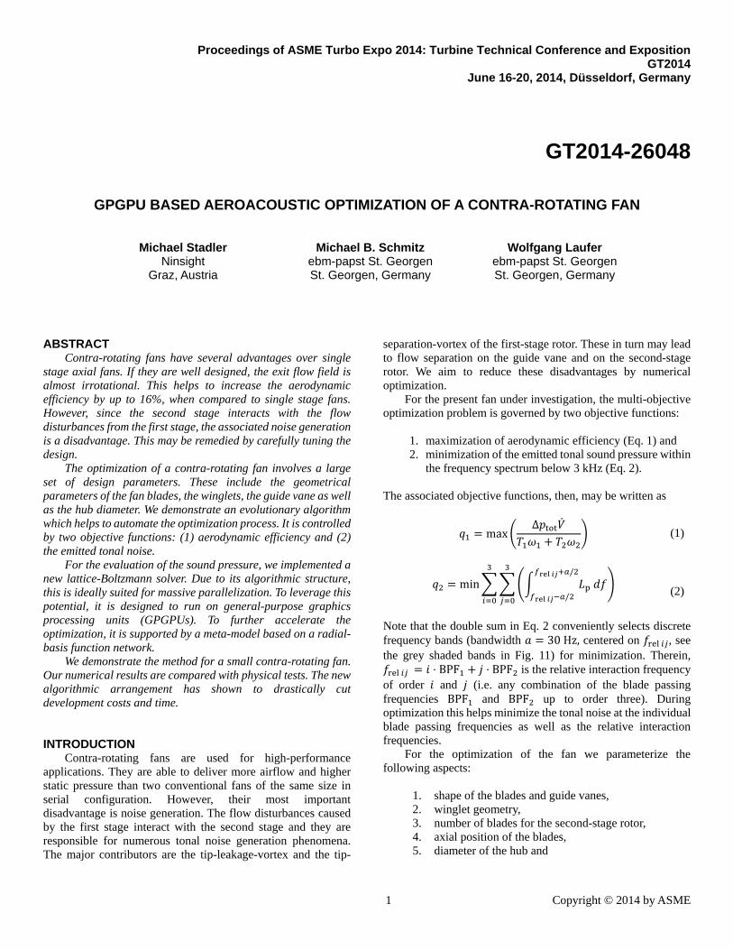
In this paper we demonstrate the entire optimization strategy for a contra-rotating fan of diameter 115 mm. The fan’s first stage consists of five blades, the second stage of a variable number of blades (see Fig. 1). To reduce tip losses, the blades are

fitted with winglets. The guide vanes are positioned between the two rotor stages. The fan is optimized for two distinct operating points: (1) 0.19, 0.45 and (2) 0.21, 0.56. Here aeroacoustic optimization is important only for the first operating point. The second operating point is the emergency operation in case of failure of one or more fans in the plant. For this mode the noise level is not important. The axial dimension of the complete fan is constrained to 83 mm.

The remaining paper is structured as follows: in the following section we introduce the parameterization of the fan geometry. Subsequently we present the LBM with brief references to implementation details for the GPGPU-based stream processor. To validate the LBM code it is benchmarked with two reference solutions. We then outline the optimization procedure. Our simulations are backed up by tests on physical specimens. The details of the testing facilities are briefly outlined in the next section. Finally we present the resulting optimal design of the contra-rotating fan. The paper concludes with an evaluation of the numerical efficiency of the presented optimization technique.

Fig. 1: The contra rotating fan to be optimized. The first-stage rotor is shown in red, the second-stage rotor in blue and the guide vanes in grey.

PARAMETERIZATION OF THE FAN GEOMETRY

In this section we outline the methods for parameterizing individual parts of an axial fan.

To make the inverse design procedure more efficient, a few general rules should be adhered to: the number of geometrical parameters should be mini-

mized,


the design space should be set up to exclude physically impossible designs.

Blade and guide vane. For the parameterization of blade

and guide vane, we describe the skeletal surface by sheets of vorticity according to [8]. Their strength is determined by a user- specified distribution of circumferentially averaged swirl ⋅

, defined as

⋅2

⋅ (3)

where is the number of blades, the radius, the circumferential velocity component and the angular coordinate in the cylindrical coordinate system. Blade loading is directly related to the meridional derivatives of ⋅ , hence

∆2 ⋅

(4)

where∆ is the pressure loading on the blade, the relative meridional blade surface velocity and refers to a derivative along (see Fig. 2) in the meridional plane.

The blade shape is obtained by alignment of its skeletal surface with the local velocity vector (i.e. imposing the inviscid slip condition). Consequently, the blade shape is controlled by only two parameters (i.e. ⋅ at the hub and at the shroud section of the trailing edge). This defines the distribution of ⋅

across the meridional section. It helps to greatly reduce the number of parameters describing the blade (as opposed to describing the blade geometry directly by a B-spline surface with associated control points as parameters). In addition, it precludes many non-physical blade geometries. For more details, see [8]. The thickness of the blade is defined by a NACA profile.

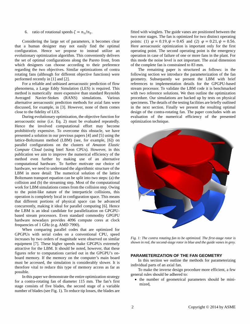
Winglet. The winglet geometry represents a helical

extrusion of the blade in the radial direction of the fan. In terms of parametric CAD, this arrangement is obtained by cutting the blade with a cylinder of diameter 0.8 ⋅ whose axis coincides with the fan axis (see Fig. 2). represents the outer diameter of the fan. We shall denote the resulting cross section by . Subsequently a second cross section is created by orthogonal projection of onto a cylindrical surface of diameter and axis . For successive shape optimization, it is convenient to

parameterize the transformations of as follows: (1) rotation about the radial axis , (2) rotation about the fan axis and (3) translation along .

The closure of the winglet surface is obtained by a multi-section extrusion between sections and (thereby enforcing continuity at the interface between the original blade and , see Fig. 2).

The winglet geometry shows an interesting shape: It curves towards the suction side at the leading edge (angle , Fig. 2) and towards the pressure side at the trailing edge (angle , Fig. 2). The detailed winglet geometry can be seen in sections A to F in Fig. 2). The curvature radius of the winglet varies along the blade, so that it resembles a number of generalized conical sections.

Fig. 2: Axis normal sections A-A to G-G illustrating the conical winglet geometry (only one blade shown).

LATTICE-BOLTZMANN METHOD

Several numerical strategies for assessing the aeroacoustic properties of an axial fan were compared in [3]. These included Large Eddy Simulation (LES), Detached Eddy Simulation (DES), Scale Adaptive Simulation (SAS) and Unsteady Reynolds Averaged Navier Stokes (URANS) simulation. SAS is an improved URANS method which introduces the Kármán


length scale into the turbulence scale equation and then dynamically adjusts the turbulence model as a function of the flow field [9]. Clearly, only LES was able to reliably predict the aeroacoustic noise of the fan. To evaluate the aeroacoustic performance of the fan under investigation in the present study, an unsteady LES solution is therefore required. This could theoretically be achieved with the Navier-Stokes (NS) equation or the LBM. The computational philosophies behind these strategies are vastly different: While the LBM leads to very simple, explicit and frequent calculations at each node, the NS-based calculation at each node is complex, implicit and occurs less frequently. At first glance, it would appear that the advantage achieved by the LBM due to the simplicity of the calculation would be offset by the higher frequency of computations, rendering the two methods equal. However, this is not the case. What sets the two methods apart is the locality of the calculations at each node. The LBM scheme leads to calculations that are not only simple but also involve only local interactions.

In the NS method, global interactions play a major role, resulting in a severe communication penalty and a marked reduction of computational speed. This difference becomes even more significant when computations are performed on multi-processor parallel platforms. The NS-based computations typically scale poorly with an increase in the number of processors. The LBM computations, on the other hand, exhibit excellent scalability characteristics.

For an efficient evaluation of the aeroacoustic objective functions during the optimization, we have implemented the LBM to run on a cluster of GPGPUs. According to the notation of Qian, the code uses the D2Q9 and D3Q19 lattices [10]. For an efficient discretization, a hierarchical mesh structure is employed according to [11] and [12]. To represent the effects of unresolved small-scale fluid motions, the Smagorinsky subgrid model is utilized [13]. For the algorithmic implementation on the GPGPU, the OpenCL [14] application programming interface was chosen.

VALIDATION OF THE LBM CODE

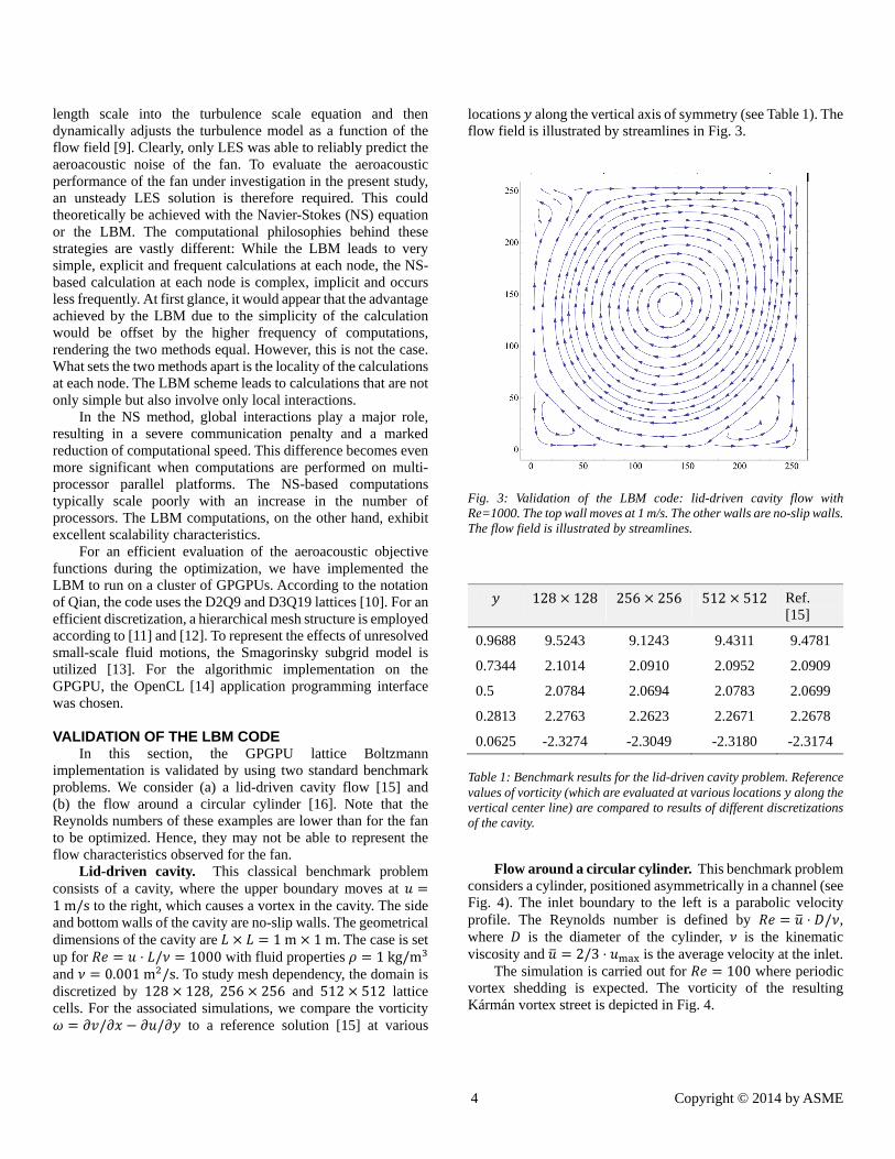
In this section, the GPGPU lattice Boltzmann implementation is validated by using two standard benchmark problems. We consider (a) a lid-driven cavity flow [15] and (b) the flow around a circular cylinder [16]. Note that the Reynolds numbers of these examples are lower than for the fan to be optimized. Hence, they may not be able to represent the flow characteristics observed for the fan.

Lid-driven cavity. This classical benchmark problem consists of a cavity, where the upper boundary moves at 1m/s to the right, which causes a vortex in the cavity. The side and bottom walls of the cavity are no-slip walls. The geometrical dimensions of the cavity are 1m 1m. The case is set up for ⋅ / 1000 with fluid properties 1kg/m and 0.001m /s. To study mesh dependency, the domain is discretized by 128 128, 256 256 and 512 512 lattice cells. For the associated simulations, we compare the vorticity

/ / to a reference solution [15] at various

locations along the vertical axis of symmetry (see Table 1). The flow field is illustrated by streamlines in Fig. 3.

Fig. 3: Validation of the LBM code: lid-driven cavity flow with Re=1000. The top wall moves at 1 m/s. The other walls are no-slip walls. The flow field is illustrated by streamlines.

128 128 256 256 512 512 Ref. [15]

0.9688 9.5243 9.1243 9.4311 9.4781

0.7344 2.1014 2.0910 2.0952 2.0909

0.5 2.0784 2.0694 2.0783 2.0699

0.2813 2.2763 2.2623 2.2671 2.2678

0.0625 -2.3274 -2.3049 -2.3180 -2.3174 Table 1: Benchmark results for the lid-driven cavity problem. Reference values of vorticity (which are evaluated at various locations along the vertical center line) are compared to results of different discretizations of the cavity.

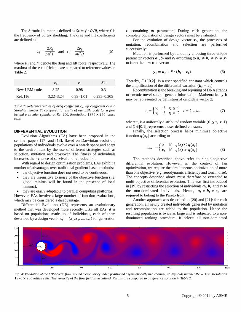
Flow around a circular cylinder. This benchmark problem considers a cylinder, positioned asymmetrically in a channel (see Fig. 4). The inlet boundary to the left is a parabolic velocity profile. The Reynolds number is defined by ⋅ / , where is the diameter of the cylinder, is the kinematic viscosity and 2/3 ⋅ is the average velocity at the inlet.

The simulation is carried out for 100 where periodic vortex shedding is expected. The vorticity of the resulting Kármán vortex street is depicted in Fig. 4.


The Strouhal number is defined as ⋅ / , where is the frequency of vortex shedding. The drag and lift coefficients are defined as

2

and2

(5)

where and denote the drag and lift force, respectively. The maxima of these coefficients are compared to reference values in Table 2.

New LBM code 3.25 0.98 0.3

Ref. [16] 3.22–3.24 0.99–1.01 0.295–0.305 Table 2: Reference values of drag coefficient , lift coefficient and Strouhal number compared to results of our LBM code for a flow behind a circular cylinder at Re=100. Resolution: 1376 256 lattice cells.

DIFFERENTIAL EVOLUTION

Evolution Algorithms (EA) have been proposed in the seminal papers [17] and [18]. Based on Darwinian evolution, populations of individuals evolve over a search space and adapt to the environment by the use of different strategies such as selection, mutation and crossover. The fitness of individuals increases their chance of survival and reproduction.

With regard to design optimization problems, EAs exhibit a number of advantages over traditional gradient-based methods: the objective function does not need to be continuous, they are insensitive to noise of the objective function (i.e.

global minima will be found in the presence of local minima),

they are easily adaptable to parallel computing platforms. However, EAs involve a large number of function evaluations, which may be considered a disadvantage.

Differential Evolution (DE) represents an evolutionary method that was developed more recently. Like all EAs, it is based on populations made up of individuals, each of them described by a design vector , , … , for generation

, containing parameters. During each generation, the complete population of design vectors must be evaluated.

For the evolution of design vector , the processes of mutation, recombination and selection are performed successively:

Mutation is performed by randomly choosing three unique parameter vectors , and according to to form the new trial vector

∙ (6) Thereby, ∈ 0,2 is a user specified constant which controls the amplification of the differential variation .

Recombination is the breaking and rejoining of DNA strands to encode novel sets of genetic information. Mathematically it may be represented by definition of candidate vector

ifif 1… (7)

where is a uniformly distributed random variable 0 1 and ∈ 0,1 represents a user defined constant.

Finally, the selection process helps minimize objective function according to

ifif

(8)

The methods described above refer to single-objective differential evolution. However, in the context of fan optimization, we require the simultaneous optimization of more than one objective (e.g. aerodynamic efficiency and tonal noise). The concepts described above must therefore be extended to multi-objective differential evolution. This was first introduced in [19] by restricting the selection of individuals , and to the non-dominated individuals. Hence, are required to belong to the Pareto front.

Another approach was described in [20] and [21]: for each generation, all newly created individuals generated by mutation and recombination are added to the population. Hence the resulting population is twice as large and is subjected to a non-dominated ranking procedure. It selects all non-dominated

Fig. 4: Validation of the LBM code: flow around a circular cylinder, positioned asymmetrically in a channel, at Reynolds number 100. Resolution: 1376 256 lattice cells. The vorticity of the flow field is visualized. Results are compared to a reference solution in Table 2.


individuals, assigns them the rank 1 and removes them from the population. The ranking procedure is repeated successively to identify individuals of higher ranks until the whole population is ranked. In a final step the original size of the population is obtained by adding individuals from ranks of increasing number, starting at rank 1. These strategies form the core of NSGA-II [21].

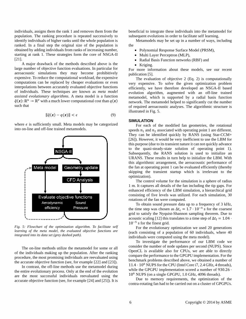
A major drawback of the methods described above is the large number of objective function evaluations. In particular for aeroacoustic simulations they may become prohibitively expensive. To reduce the computational workload, the expensive computations can be replaced by cheaper evaluations or even interpolations between accurately evaluated objective functions of individuals. These techniques are known as meta model assisted evolutionary algorithms. A meta model is a function

: → with a much lower computational cost than such that

‖ ‖ (9)

where is sufficiently small. Meta models may be categorized into on-line and off-line trained metamodels.

Fig. 5: Flowchart of the optimization algorithm. To facilitate self learning of the meta model, the evaluated objective functions are integrated into its data set (grey dashed path).

The on-line methods utilize the metamodel for some or all

of the individuals making up the population. After the ranking procedure, the most promising individuals are reevaluated using the accurate objective function (see, for example [22] and [23]).

In contrast, the off-line methods use the metamodel during the entire evolutionary process. Only at the end of the evolution are the most successful individuals reevaluated using the accurate objective function (see, for example [24] and [25]). It is

beneficial to integrate these individuals into the metamodel for subsequent evolutions in order to facilitate self learning.

Metamodels may be set up in a number of ways, including the

Polynomial Response Surface Model (PRSM), Multi Layer Perceptron (MLP), Radial Basis Function networks (RBF) and Kriging.

For more information about these models, see our recent publication [5].

The evaluation of objective 2 (Eq. 2) is computationally very expensive. To solve the given optimization problem efficiently, we have therefore developed an NSGA-II based evolution algorithm, augmented with an off-line trained metamodel, which is supported by a radial basis function network. The metamodel helped to significantly cut the number of required aeroacoustic analyses. The algorithmic structure is illustrated in Fig. 5.

SIMULATION For each of the modified fan geometries, the rotational

speeds and associated with operating point 1 are different. They can be identified quickly by RANS (using Star-CCM+ [26]). However, it would be very inefficient to use the LBM for this purpose (due to its transient nature it can not quickly advance to the quasi-steady-state solution of operating point 1). Subsequently, the RANS solution is used to initialize an URANS. These results in turn help to initialize the LBM. With this algorithmic arrangement, the aeroacoustic performance of the fan at operating point 1 can be evaluated efficiently (thereby skipping the transient startup which is irrelevant to the optimization).

The control volume for the simulation is a sphere of radius 1 m. It captures all details of the fan including the tip gaps. For enhanced efficiency of the LBM simulation, a hierarchical grid consisting of five levels was utilized. For each simulation, 30 rotations of the fan were computed.

To obtain sound pressure data up to a frequency of 3 kHz, the time step was chosen as Δ 1.7 ⋅ 10 s for the coarsest grid to satisfy the Nyquist-Shannon sampling theorem. Due to acoustic scaling [12] this translates to a time step of Δ 1.04 ⋅10 s for the finest grid.

For the evolutionary optimization we used 20 generations (each consisting of a population of 60 individuals, where 40 individuals were computed using the meta model).

To investigate the performance of our LBM code we consider the number of node updates per second (NUPS). Since OpenCL is available also for CPUs, we are able to directly compare the performance to the GPGPU implementation. For the benchmark problems described above, we obtained a number of 11.4 ⋅ 10 NUPS for the CPU (Intel Core i7, 2.4 GHz, 4 threads), while the GPGPU implementation scored a number of 930.26 ⋅10 NUPS (on a single GPGPU, 1.0 GHz, 4096 threads).

Due to memory requirements, the optimization of the contra-rotating fan had to be carried out on a cluster of GPGPUs.


The communication between these individual processors significantly degraded the performance down to 138.30 ⋅ 10 NUPS per GPGPU (largely depending on the nature of the problem). To control the optimization the mathematical model was realized using the software Mathematica.

EXPERIMENTAL SET-UP From experiments we obtain fan charts and the sound power

level. To facilitate testing of arbitrary configurations, a modular test set-up consisting of the following five fan components was designed: (1) casing 1, (2) rotor 1, (3) rotor 2 and (4) casing 2 and (5) guide vanes. Each of these components can be changed individually to study its particular influence on the overall performance. Components (1)–(4) are made by rapid prototyping. The guide vanes are milled from aluminum.

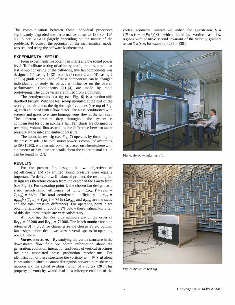
The aerodynamics test rig (see Fig. 6) is a suction-side throttled facility. With the test set-up mounted at the exit of the test rig, the air enters the rig through five tubes (see top of Fig. 6), each equipped with a flow meter. The air is conditioned with screens and gazes to ensure homogeneous flow at the fan inlet. The inherent pressure drop throughout the system is compensated for by an auxiliary fan. Fan charts are obtained by recording volume flux as well as the difference between static pressure at the inlet and ambient pressure.

The acoustics test rig (see Fig. 7) operates by throttling on the pressure side. The total sound power is computed according to ISO 10302, with ten microphones placed on a hemisphere with a diameter of 2 m. Further details about the experimental set-up can be found in [27].

RESULTS For the present fan design, the two objectives of

(a) efficiency and (b) emitted sound pressure were equally important. To deliver a well-balanced product, the resulting fan design was therefore chosen from the center of the Pareto front (see Fig. 9). For operating point 1, the chosen fan design has a static aerodynamic efficiency of Δ /

66%. The total aerodynamic efficiency is Δ / 76% (Δ and Δ are the static and the total pressure difference). For operating point 2 we obtain efficiencies of about 0.3% below these values. For a fan of this size, these results are very satisfactory.

At rotor tip, the Reynolds numbers are of the order of Re 93000 and Re 71000. The Mach-number for both rotors is 0.08. To characterize the chosen Pareto optimal fan design in more detail, we assess several aspects for operating point 1 below.

Vortex structure. By studying the vortex structure in the downstream flow field we obtain information about the generation, evolution, interaction and decay of vortical structures including associated noise production mechanisms. For identification of these structures the vorticity | | alone is not suitable since it cannot distinguish between pure shearing motions and the actual swirling motion of a vortex [28]. This property of vorticity would lead to a misrepresentation of the

vortex geometry. Instead we utilize the Q-criterion ⋅ tr /2, which identifies vortices as flow

regions with positive second invariant of the velocity gradient tensor (see, for example, [29] or [30]).

Fig. 6: Aerodynamics test rig.

Fig. 7: Acoustics test rig.


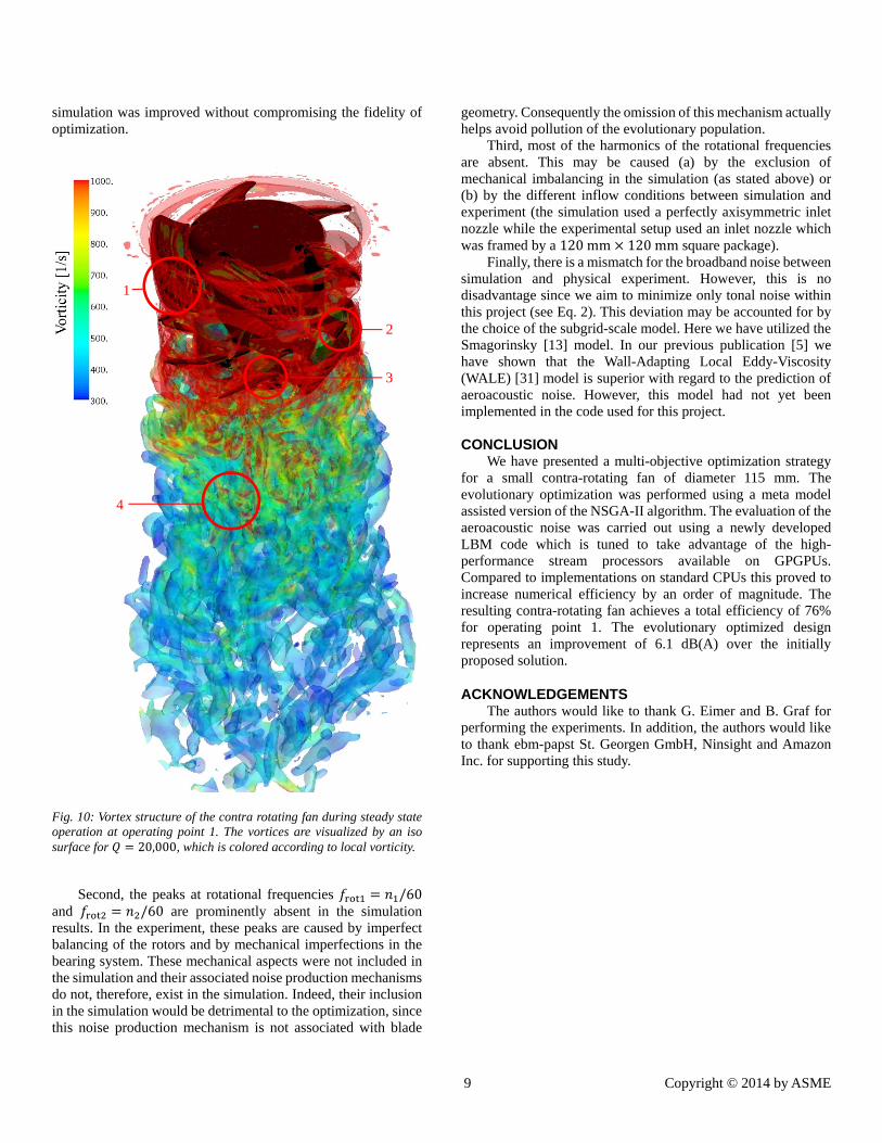
The resulting isosurface is displayed for Q-criterion 20,000, which is colored by the local vorticity (see Fig. 10). It shows the generation of tip vortices in the first-stage rotor (Fig. 10, item 1) as well as their interaction with the guide vanes (Fig. 10, item 2) and with the second-stage rotor (Fig. 10, item 3). The latter is the source of peaks in the acoustic frequency spectrum at the relative interaction frequencies (see Fig. 11).

Fig. 9: Objective space for optimization, showing the evolution of the population. Generations G5 to G20 are shown in distinct colors. The Pareto front is shown as a black dashed line. The optimum candidate chosen for the final product is indicated by a red star symbol. The sound pressure level is given relative to a fixed reference (see also Fig. 11).

Tangential velocity. Any non-axial flow component in the exit flow field represents an energy loss. For a high-efficiency design of the fan, the tangential velocity at the outlet should

therefore be as small as possible. The visualization clearly indicates the absence of any tangential large scale vortices in the downstream flow field (Fig. 10, item 4). In particular, results show that the maximum tangential velocity in the exit flow field is 1.6m/s. To put that into context, the circumferential velocity of the first-stage rotor at operating point 1 is 26m/s. Hence, / 0.06. This represents a very favorable result compared to similar designs. Hence, the losses due to circulation in the exit flow field are negligible.

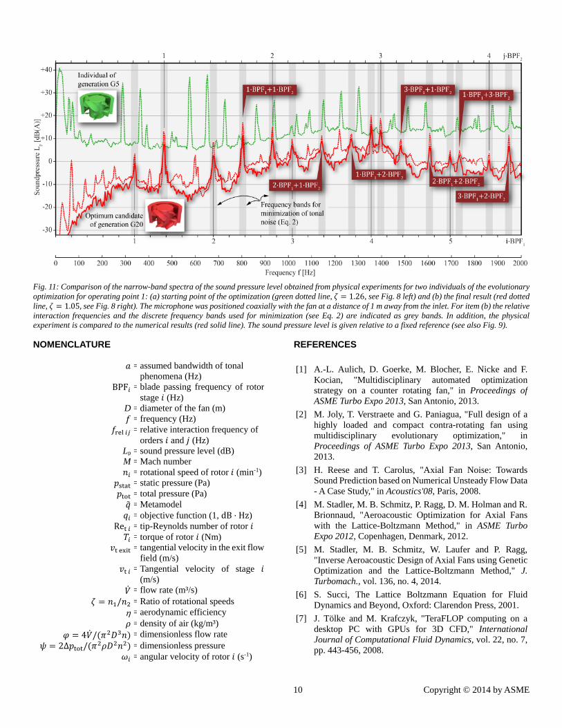
Acoustic frequency spectrum. To study the agreement between simulation and physical experiment we compare their resulting acoustic narrow-band spectra in Fig. 11. Clearly, both simulation and experiment show peaks at coinciding locations for the blade passing frequencies as well as their associated harmonics ⋅ BPF and ⋅ BPF with , .

Furthermore, we observe additional peaks at the relative interaction frequencies ⋅ BPF ⋅ BPF with , . These are attributed to pressure fluctuations caused by interactions between the first- and the second-stage rotor. The associated vortex (i.e. the first-stage tip vortex interacting with the second-stage rotor) is illustrated in Fig. 10, item 3.

In general there is good agreement between simulation and physical experiment regarding the frequencies of ⋅ BPF , ⋅BPF and . However, there is a mismatch for the total noise of 4.9 dB(A) between simulation and experiment. The possible reasons for this are summarized below:

First, the amplitudes of the peaks at the relative interaction frequencies do not match. However, we were able to show that this may be remedied by choosing an increased time resolution for the simulation. For the present optimization this is not necessary since we are not interested in the absolute values of the amplitudes of the peaks. Instead, it suffices to obtain information about the relative merits of various fan designs. By choosing a lower time resolution, therefore, the efficiency of the

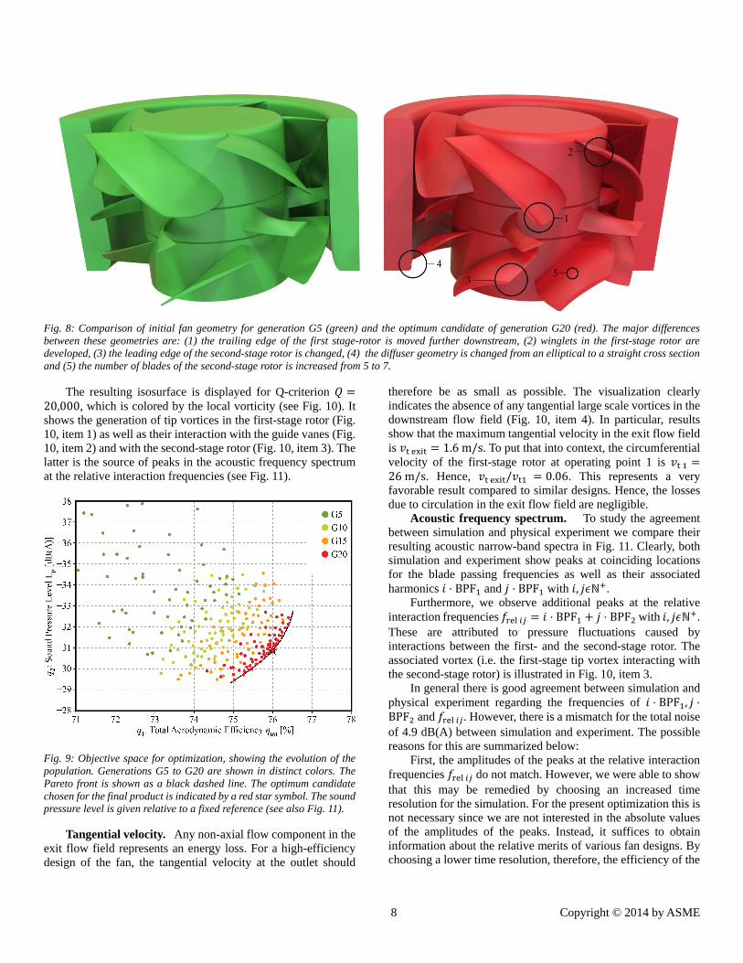
Fig. 8: Comparison of initial fan geometry for generation G5 (green) and the optimum candidate of generation G20 (red). The major differences between these geometries are: (1) the trailing edge of the first stage-rotor is moved further downstream, (2) winglets in the first-stage rotor are developed, (3) the leading edge of the second-stage rotor is changed, (4) the diffuser geometry is changed from an elliptical to a straight cross section and (5) the number of blades of the second-stage rotor is increased from 5 to 7.


simulation was improved without compromising the fidelity of optimization.

Fig. 10: Vortex structure of the contra rotating fan during steady state operation at operating point 1. The vortices are visualized by an iso surface for 20,000, which is colored according to local vorticity.

Second, the peaks at rotational frequencies /60

and /60 are prominently absent in the simulation results. In the experiment, these peaks are caused by imperfect balancing of the rotors and by mechanical imperfections in the bearing system. These mechanical aspects were not included in the simulation and their associated noise production mechanisms do not, therefore, exist in the simulation. Indeed, their inclusion in the simulation would be detrimental to the optimization, since this noise production mechanism is not associated with blade

geometry. Consequently the omission of this mechanism actually helps avoid pollution of the evolutionary population.

Third, most of the harmonics of the rotational frequencies are absent. This may be caused (a) by the exclusion of mechanical imbalancing in the simulation (as stated above) or (b) by the different inflow conditions between simulation and experiment (the simulation used a perfectly axisymmetric inlet nozzle while the experimental setup used an inlet nozzle which was framed by a 120mm 120mm square package).

Finally, there is a mismatch for the broadband noise between simulation and physical experiment. However, this is no disadvantage since we aim to minimize only tonal noise within this project (see Eq. 2). This deviation may be accounted for by the choice of the subgrid-scale model. Here we have utilized the Smagorinsky [13] model. In our previous publication [5] we have shown that the Wall-Adapting Local Eddy-Viscosity (WALE) [31] model is superior with regard to the prediction of aeroacoustic noise. However, this model had not yet been implemented in the code used for this project.

CONCLUSION

We have presented a multi-objective optimization strategy for a small contra-rotating fan of diameter 115 mm. The evolutionary optimization was performed using a meta model assisted version of the NSGA-II algorithm. The evaluation of the aeroacoustic noise was carried out using a newly developed LBM code which is tuned to take advantage of the high-performance stream processors available on GPGPUs. Compared to implementations on standard CPUs this proved to increase numerical efficiency by an order of magnitude. The resulting contra-rotating fan achieves a total efficiency of 76% for operating point 1. The evolutionary optimized design represents an improvement of 6.1 dB(A) over the initially proposed solution.

ACKNOWLEDGEMENTS The authors would like to thank G. Eimer and B. Graf for

performing the experiments. In addition, the authors would like to thank ebm-papst St. Georgen GmbH, Ninsight and Amazon Inc. for supporting this study.

1

2

3

4


NOMENCLATURE

= assumed bandwidth of tonal phenomena (Hz)

BPF = blade passing frequency of rotorstage (Hz)

D = diameter of the fan (m) = frequency (Hz)

= relative interaction frequency of orders and (Hz)

Lp = sound pressure level (dB) M = Mach number

= rotational speed of rotor (min-1)= static pressure (Pa) = total pressure (Pa) = Metamodel = objective function (1, dB ⋅ Hz)

Re = tip-Reynolds number of rotor = torque of rotor (Nm)

= tangential velocity in the exit flowfield (m/s)

= Tangential velocity of stage (m/s)

= flow rate (m³/s) / = Ratio of rotational speeds = aerodynamic efficiency

= density of air (kg/m³) 4 / = dimensionless flow rate

2Δ / = dimensionless pressure = angular velocity of rotor (s-1)

REFERENCES [1] A.-L. Aulich, D. Goerke, M. Blocher, E. Nicke and F.

Kocian, "Multidisciplinary automated optimization strategy on a counter rotating fan," in Proceedings of ASME Turbo Expo 2013, San Antonio, 2013.

[2] M. Joly, T. Verstraete and G. Paniagua, "Full design of a highly loaded and compact contra-rotating fan using multidisciplinary evolutionary optimization," in Proceedings of ASME Turbo Expo 2013, San Antonio, 2013.

[3] H. Reese and T. Carolus, "Axial Fan Noise: Towards Sound Prediction based on Numerical Unsteady Flow Data - A Case Study," in Acoustics'08, Paris, 2008.

[4] M. Stadler, M. B. Schmitz, P. Ragg, D. M. Holman and R. Brionnaud, "Aeroacoustic Optimization for Axial Fans with the Lattice-Boltzmann Method," in ASME Turbo Expo 2012, Copenhagen, Denmark, 2012.

[5] M. Stadler, M. B. Schmitz, W. Laufer and P. Ragg, "Inverse Aeroacoustic Design of Axial Fans using Genetic Optimization and the Lattice-Boltzmann Method," J. Turbomach., vol. 136, no. 4, 2014.

[6] S. Succi, The Lattice Boltzmann Equation for Fluid Dynamics and Beyond, Oxford: Clarendon Press, 2001.

[7] J. Tölke and M. Krafczyk, "TeraFLOP computing on a desktop PC with GPUs for 3D CFD," International Journal of Computational Fluid Dynamics, vol. 22, no. 7, pp. 443-456, 2008.

Fig. 11: Comparison of the narrow-band spectra of the sound pressure level obtained from physical experiments for two individuals of the evolutionaryoptimization for operating point 1: (a) starting point of the optimization (green dotted line, 1.26, see Fig. 8 left) and (b) the final result (red dottedline, 1.05, see Fig. 8 right). The microphone was positioned coaxially with the fan at a distance of 1 m away from the inlet. For item (b) the relative interaction frequencies and the discrete frequency bands used for minimization (see Eq. 2) are indicated as grey bands. In addition, the physical experiment is compared to the numerical results (red solid line). The sound pressure level is given relative to a fixed reference (see also Fig. 9).


[8] M. Zangeneh and M. de Maillard, "Optimization of Fan Noise by Coupling 3D Inverse Design and Automatic Optimizer," in Proceedings of Fan 2012, Senlis, France, 2012.

[9] F. R. Menter and Y. Egorov, "The Scale-Adaptive Simulation Method for Unsteady Turbulent Flow Predictions. Part 1: Theory and Model Description," Flow, Turbulence and Combustion, vol. 85, no. 1, pp. 113-138, 2010.

[10] Y. H. Qian, D. d'Humières and P. Lallemand, "Lattice BGK models for Navier-Stokes equation," Europhysics Letters (EPL), vol. 17, no. 6, pp. 479-484, 1992.

[11] R. Freitas, M. Meinke and W. Schröder, "Turbulence simulation via the Lattice-Boltzmann method on hierarchically refined meshes," in European Conference on Computational Fluid Dynamics ECCOMAS CFD 2006, Delft, The Netherlands, 2006.

[12] M. Schönherr, K. Kucher, M. Geier, M. Stiebler, S. Freudiger and M. Krafczyk, "Multi-thread implementation of the lattice Boltzmann method on non-uniform grids for CPUs and GPUs," Computers & Mathematics with Applications, vol. 61, no. 1, pp. 3730-3743, 2011.

[13] J. Smagorinsky, "General circulation experiments with the primitive equations. 1. The basic experiment," Mon. Weather Rev., vol. 91, pp. 99-164, 1963.

[14] Khronos Group, OpenCL 2.0 Programming Guide, Beaverton, Oregon: Khronos Group, 2013.

[15] C.-H. Bruneau and M. Saad, "The 2D lid-driven cavity problem revisited," Computers & Fluids, vol. 35, pp. 326-348, 2006.

[16] M. Schäfer and S. Turek, "Benchmark computations of laminar flow around cylinder," Notes on Numerical Fluid Mechanics, no. 52, pp. 547-566, 1996.

[17] J. Holland, Adaptation in Natural and Artificial Systems, University of Michigan Press, 1975.

[18] I. Rechenberg, Optimierung technischer Systeme nach Prinzipien der biologischen Evolution, Stuttgart: Frommann-Holzboog, 1973.

[19] H. Abbas, R. Sarker and C. Newton, "PDE: A Pareto-Frontier Differential Evolution Approach for Multi-Objective Optimization Problems," in Proceedings of the Congress on Evolutionary Computation, Piscataway, New Jersey, 2001.

[20] N. Madavan, "Multiobjective Optimization using a Pareto Differential Evolution Approach," in Proceedings of the Congress on Evolutionary Computation, Honolulu, Hawaii, 2002.

[21] K. Deb, S. Agrawal, A. Pratap and T. Meyarivan, "A fast elitist Non-Dominated Sorting Genetic Algorithm for Multi-Objective Optimization: NSGA-II," in Proceedings of the Parallel Problem Solving from Nature VI Conference, Paris, France, 2000.

[22] K. Giannakoglou and M. Karakasis, "Hierarchical and Distributed Metamodel-Assisted Evolutionary Algorithms," in VKI Lecture Series on Introduction to Optimization and Multidisiplinary Design, Brussels, 2006.

[23] M. Karakasis, K. Giannakoglou and D. Koubogiannis, "Aerodynamic Design of Compressor Airfoils using Hierarchical, Distributed Metamodel-Assisted Evolutionary Algorithms," in 7th European Conference on Turbomachinery, Fluid Dynamics and Thermodynamics, Athens, 2007.

[24] S. Pierret, "Designing Turbo machinery Blades by means of the Function Approximation Concept based on Artificial Neural Network, Genetic Algorithm and the Navier-Stokes Equations," Ph.D. Thesis, Faculte Polytechnique de Mons, 1999.

[25] T. Verstraete, "Multidisciplinary Turbo Machinery Component Optimization Considering Performance, Stress and Internal Heat Transfer," University of Ghent, Ph.D. Thesis, 2008.

[26] cd-adapco, Star-CCM+ User Manual, 2013.

[27] M. B. Schmitz, G. Eimer and H. Schmid, "Design and test of a small high performance diagonal fan," in Proceedings of ASME Turbo Expo 2011, Vancouver, Canada, 2011.

[28] V. Kolár, "Vortex identification: New requirements and limitations," Int. J. of Heat and Fluid Flow, vol. 28, pp. 638-652, 2007.

[29] P. Chakraborty, S. Balachandar and R. Adrian, "On the relationships between local vortex identification schemes," J. Fluid Mech., vol. 535, pp. 189-214, 2005.

[30] G. Haller, "An objective definition of a vortex," J. Fluid Mech., vol. 525, pp. 1-26, 2005.

[31] F. Ducros, F. Nicoud and T. Poinsot, "Wall-adapting local eddy-viscosity models for simulations in complex geometries," in Proceedings Conf. on Num. Meth. Fluid Dyn., Oxford, UK, 1998.

Documents

ASME TurboExpo2014 FinalSubmission