Asking the Right Question: Risk and Expectation

in Multi-Agent Contracting

Alexander Babanov, John Collins, and Maria GiniDepartment of Computer Science and Engineering

University of Minnesota

Keywords: Automated auctions, multi-agent contracting, expected utility, risk estimation, optimization

Abstract

This paper investigates methods of reducing risk in market-based auctions of tasks with complex time

constraints and interdependencies. The research addresses problems in a contracting setting in which

a buyer has a set of tasks to be performed. Because of the complex dependencies among the tasks, a

task not completed on time might have devastating effect on other tasks. Therefore, the problem is to

sequence tasks and allocate time windows to maximize the expected utility of the agent. Because there is

a probability of loss as well as a probability of gain, the decision process must deal with the risk posture

of the person or organization on whose behalf the decision maker is acting.

1 Introduction

E-commerce technology has the potential to benefit society by reducing the cost of buying and selling andby opening new market opportunities. The main domain of application we envision is the management ofagile and dynamic supply-chains, an area in which the potential payoff is high, given the projected size ofthe business-to-business and make-to-order e-commerce markets.

More production processes are being outsourced to outside contractors, making supply chains longer and moreconvoluted. This increased complexity is compounded by increasing competitive pressure, and acceleratedproduction schedules which demand tight integration of all processes.

Finding potential suppliers is only a step in the process of producing goods. Time dependencies amongoperations make scheduling a major factor. A late delivery of a part might produce a cascade of devastatingeffects. Unfortunately, current auction-based systems do not have any notion of time. Handling auctions fortasks with time constraints is beyond the capabilities of current e-commerce systems.

We present the results of a study of how an autonomous agent can maximize its profits while predicting andmanaging its financial risk exposure when requesting bids for tasks with complex time constraints. We showhow this can be done by specifying appropriate time windows for tasks when soliciting bids, and by usingreceived bids effectively in building a final work schedule.

1

This study is a part of the MAGNET (Multi-AGent NEgotiation Testbed) research project. MAGNETagents participate in first-price, sealed-bid combinatorial auctions over collections of tasks with precedencerelations and time constraints. MAGNET promises to increase the efficiency of current markets by shiftingmuch of the burden of market exploration, auction handling, and preliminary decision analysis from humandecision makers to a network of heterogeneous agents.

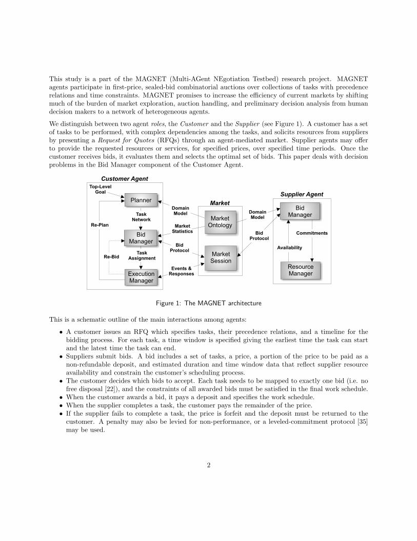
We distinguish between two agent roles, the Customer and the Supplier (see Figure 1). A customer has a setof tasks to be performed, with complex dependencies among the tasks, and solicits resources from suppliersby presenting a Request for Quotes (RFQs) through an agent-mediated market. Supplier agents may offerto provide the requested resources or services, for specified prices, over specified time periods. Once thecustomer receives bids, it evaluates them and selects the optimal set of bids. This paper deals with decisionproblems in the Bid Manager component of the Customer Agent.

Figure 1: The MAGNET architecture

This is a schematic outline of the main interactions among agents:

• A customer issues an RFQ which specifies tasks, their precedence relations, and a timeline for thebidding process. For each task, a time window is specified giving the earliest time the task can startand the latest time the task can end.

• Suppliers submit bids. A bid includes a set of tasks, a price, a portion of the price to be paid as anon-refundable deposit, and estimated duration and time window data that reflect supplier resourceavailability and constrain the customer’s scheduling process.

• The customer decides which bids to accept. Each task needs to be mapped to exactly one bid (i.e. nofree disposal [22]), and the constraints of all awarded bids must be satisfied in the final work schedule.

• When the customer awards a bid, it pays a deposit and specifies the work schedule.• When the supplier completes a task, the customer pays the remainder of the price.• If the supplier fails to complete a task, the price is forfeit and the deposit must be returned to the

customer. A penalty may also be levied for non-performance, or a leveled-commitment protocol [35]may be used.

2

1.1 A Motivating Example

As an example, imagine that we need to construct a garage. Figure 2 shows the tasks needed to completethe construction. The tasks are represented in a task network, where links indicate precedence constraints.The first decision we are faced with is how to sequence the tasks in the RFQ and how much time to allocateto each of them. For instance, we could reduce the number of parallel tasks, allocate more time to tasks withhigher variability in duration or tasks for which there is a shortage of laborers, or allow more slack time.

Roofing

Masonry InteriorPlumbing

Electric

Exterior

2

3

4

1 5 6

1086420week

Roofing

Interior

Masonry

Exterior

Electric

Plumbing

Figure 2: A task network example and the corresponding RFQ.

A sample RFQ is shown in Figure 2. Note that the time windows in the RFQ do not need to obey theprecedence constraints; the only requirement is that the accepted bids obey them. We assume that thesupplier is more likely to bid, and submit a lower-cost bid, if it is given a greater flexibility in scheduling itsresources.

1.2 Experiences and Open Issues

We have shown [3] that the time constraints specified in the RFQ can affect the customer’s outcome in twomajor ways:

1. by affecting the number, price, and time windows of bids. We assume that bids will reflect supplierresource commitments, and therefore larger time windows will result in more bids and better utilizationof resources, in turn leading to lower prices [5]. However, an RFQ with overlapping time windows makesthe process of winner determination more complex [4]. Another less obvious problem is that everyextra bid over the minimum needed to cover all tasks adds one more rejected bid. Ultimately, a largepercentage of rejections will reduce the customer agent’s credibility, which, after repeated interactionsin the market, will result in fewer bids and/or higher costs.

2. by affecting the financial exposure of the customer agent [3]. We assume non-refundable deposits arepaid to secure awarded bids, and payments for each task are made as the tasks are completed. Thepayoff for the customer occurs only at the completion of all the tasks. Once a task is completed inthe time period specified, the customer is liable for its full cost, regardless of whether in the meantimeother tasks have failed. If a task is not completed by the supplier, the customer is not liable for itscost, but this failure can ruin other parts of the plan. Slack in the schedule increases the probabilitythat tasks will be completed or that there will be enough time to recover if any fail. However, slack

3

extends the completion time and so reduces the payoff. In made-to-order products the speed is thekey; the value of the final payoff may drop off very steeply with time.

Because there is a probability of loss as well as a probability of gain, we must deal with the risk posture ofthe person or organization on whose behalf the agent is acting. We need a principled method for generatingRFQs that models and makes effective use of this risk posture, using both experience and available marketinformation.

2 Expected Utility Approach to Generating Optimal RFQ

In this section we describe a new approach to the construction of optimal RFQs that employs the ExpectedUtility Theory to reduce the likelihood of receiving unattractive bids, while maximizing the number of bidsthat are likely to be awarded. We pay special attention to the relation between the size of RFQ timewindows and the number of expected bids by investigating the balance between the quantity and the qualityof expected bids.

2.1 Terminology

A task network (see Figure 2) is a tuple 〈N,≺〉 of a set N of individual tasks and strict partial ordering onthem. We also use N to denote the number of tasks where appropriate.

A task network is characterized by a start time ts and a finish time tf , which delimit the interval of timewhen tasks can be scheduled. The placement of task n in the schedule is characterized by task n start timetsn and task n finish time tfn, subject to the following constraints:

ts ≤ tfm ≤ tsn, ∀m ∈ P1 (n) and tfn ≤ tsm ≤ tf ∀m ∈ S1 (n)

where P1 (n) is the a set of immediate predecessors of n, P1 (n) = {m ∈ N | m ≺ n, ∄m′ ∈ N,m ≺ m′ ≺ n}.S1 (n) is defined similarly to be the set of immediate successors of task n.

The probability of task n completion by time t, conditional on the ultimate successful completion of taskn, is distributed according to the cumulative distribution function (CDF) Φn = Φn (tsn; t) ,Φn (·;∞) = 1.Observe that Φn is defined to be explicitly dependent on the start time tsn. To see the rationale, consider theprobability of successful mail delivery in x days for packages that were mailed on different days of a week.

There is an associated unconditional probability of success pn ∈ [0, 1] characterizing the percentage of tasksthat are successfully completed given infinite time (see Figure 3).

Task n bears an associated cost1. We assume the total cost of task n has two parts: a deposit, which ispaid when the bid is accepted, and a cost cn which is due some time after successful completion of n. Inthis analysis we will not compare plans with different deposits, so we assume without loss of generality thedeposit to be 0.

There is a single final reward V scheduled at the plan finish time tf and paid conditional on all tasks in Nbeing successfully completed by that time.

1Hereafter we use words “cost” and “reward” to denote some monetary value, while referring the same value as “payoff” or

“payment” whenever it is scheduled at some time t.

4

1pn

t

pnΦn(tsn; t)

Figure 3: Unconditional distribution for successful completion probability.

There is an associated rate of return qn2 that is used to calculate the discounted present value (PV) for

payoff cn due at time t as

PV (cn; t) := cn (1 + qn)−t

.

We associate the return q with the final reward V .

2.2 Expected Utility and Certainty Equivalent

We represent the customer agent’s preferences over payoffs by the von Neumann-Morgenstern utility functionu [19]. We further assume that the absolute risk-aversion coefficient r := −u′′/u′ of u is constant for anyvalue of its argument, hence u can be represented as follows:

u (x) = − exp {−rx} for r 6= 0 and u (x) = x for r = 0

A gamble is a set of payoff-probability pairs G = {(xi, pi)i} s.t. pi > 0,∀i and∑

i pi = 1. The expectationof the utility function over a gamble G is the expected utility (EU):

Eu [G] :=∑

(xi,pi)∈G

piu (xi)

The certainty equivalent (CE) of a gamble G is defined as the single payoff value whose utility matches theexpected utility of the entire gamble G, i.e. u (CE [G]) := Eu [G]. Hence under our assumptions

CE(G) =−1

rlog

∑

(xi,pi)∈G

pi exp {−rxi} for r 6= 0 and CE(G) =∑

(xi,pi)∈G

pixi for r = 0

Naturally, the agent will not be willing to accept gambles with negative certainty equivalent, and the highervalues of the certainty equivalent will correspond to more attractive gambles.

To illustrate the concept, Figure 4 shows how the certainty equivalent depends on the risk-aversity r of anagent. In this figure we consider a gamble that brings the agent either 100 or nothing with equal probabilities.Agents with positive r’s are risk-averse; those with negative r’s are risk-loving. Agents with risk-aversityclose to zero, i.e. almost risk-neutral, have a CE equal to its weighted mean 50.

2The reason for having multiple qn’s is that individual tasks can be financed from different sources, thus affecting task

scheduling.

5

−0.1 −0.05 0 0.05 0.10

25

50

75

100

r

CE({(100,1/2),(0,1/2)})

Figure 4: Certainty equivalent of a simple gamble as a function of the risk-aversity.

2.3 Cumulative Probabilities

To compute the certainty equivalent of a gamble we need to determine a schedule for the tasks and computethe payoff probability pairs.

We assume that the payoff cn for task n is scheduled at tfn, so its present value cn3 is

cn := cn (1 + qn)−tf

n

We define the conditional probability of task n success as

pn := pnΦn

(

tsn; tfn)

.

We also define the precursors of task n as a set of tasks that finish before task n starts in a schedule, i.e.

P (n) :={

m ∈ N |tfm ≤ tsn}

.

The unconditional probability that task n will be completed successfully is

pcn = pn ×

∏

m∈P (n)

pm.

That is, the probability of successful completion of every precursor and of task n itself are consideredindependent events. The reason this is calculated in such form is because, if any task in P (n) fails to becompleted, there is no need to execute task n.

The probability of receiving the final reward V is therefore

p =∏

n∈N

pn.

3Hereafter we “wiggle” variables that depend on the current task schedule, while omitting all corresponding indices for the

sake of simplicity.

6

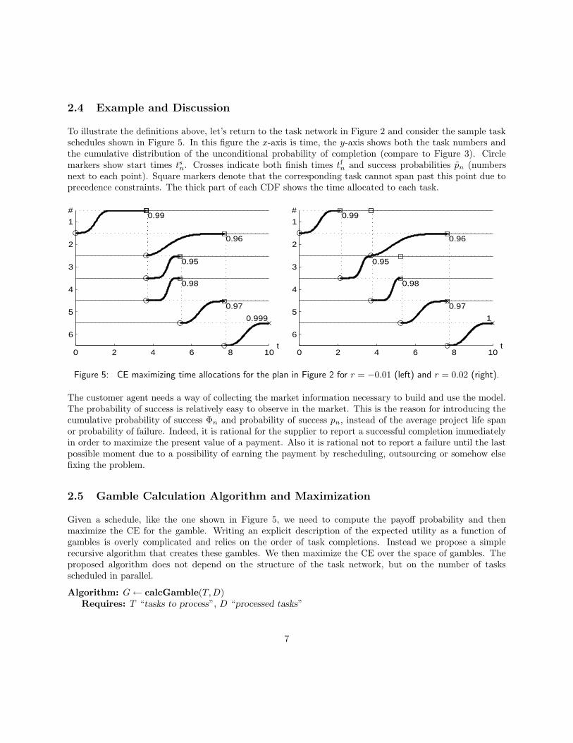
2.4 Example and Discussion

To illustrate the definitions above, let’s return to the task network in Figure 2 and consider the sample taskschedules shown in Figure 5. In this figure the x-axis is time, the y-axis shows both the task numbers andthe cumulative distribution of the unconditional probability of completion (compare to Figure 3). Circlemarkers show start times tsn. Crosses indicate both finish times tfn and success probabilities pn (numbersnext to each point). Square markers denote that the corresponding task cannot span past this point due toprecedence constraints. The thick part of each CDF shows the time allocated to each task.

0 2 4 6 8 10

1

2

3

4

5

6

0.99

0.96

0.95

0.98

0.97

0.999

#

t0 2 4 6 8 10

1

2

3

4

5

6

0.99

0.96

0.95

0.98

0.97

1

#

t

Figure 5: CE maximizing time allocations for the plan in Figure 2 for r = −0.01 (left) and r = 0.02 (right).

The customer agent needs a way of collecting the market information necessary to build and use the model.The probability of success is relatively easy to observe in the market. This is the reason for introducing thecumulative probability of success Φn and probability of success pn, instead of the average project life spanor probability of failure. Indeed, it is rational for the supplier to report a successful completion immediatelyin order to maximize the present value of a payment. Also it is rational not to report a failure until the lastpossible moment due to a possibility of earning the payment by rescheduling, outsourcing or somehow elsefixing the problem.

2.5 Gamble Calculation Algorithm and Maximization

Given a schedule, like the one shown in Figure 5, we need to compute the payoff probability and thenmaximize the CE for the gamble. Writing an explicit description of the expected utility as a function ofgambles is overly complicated and relies on the order of task completions. Instead we propose a simplerecursive algorithm that creates these gambles. We then maximize the CE over the space of gambles. Theproposed algorithm does not depend on the structure of the task network, but on the number of tasksscheduled in parallel.

Algorithm: G ← calcGamble(T,D)Requires: T “tasks to process”, D “processed tasks”

7

Returns: G “subtree gamble”

M ← {m ∈ T |P (m) ⊂ D}if M 6= ∅ “it’s a branch”

n ← first{M} “according to some ordering”T ← T \ {n}G ← ∅E ← calcGamble(T,D) “follow . . . → n path”forall (x, p) ∈ E

G ← G ∪ {(x, p × (1 − pn)})endfor

I ← calcGamble(T,D ∪ {n}) “follow . . . → n path”forall (x, p) ∈ I

G ← G ∪ {(x + cn, p × pn)}endfor

return G “subtree is processed”else “it’s a leaf ”

if N = D “all tasks are done”return {(V, 1)}

else “some task failed”return {(0, 1)}

endif

endif

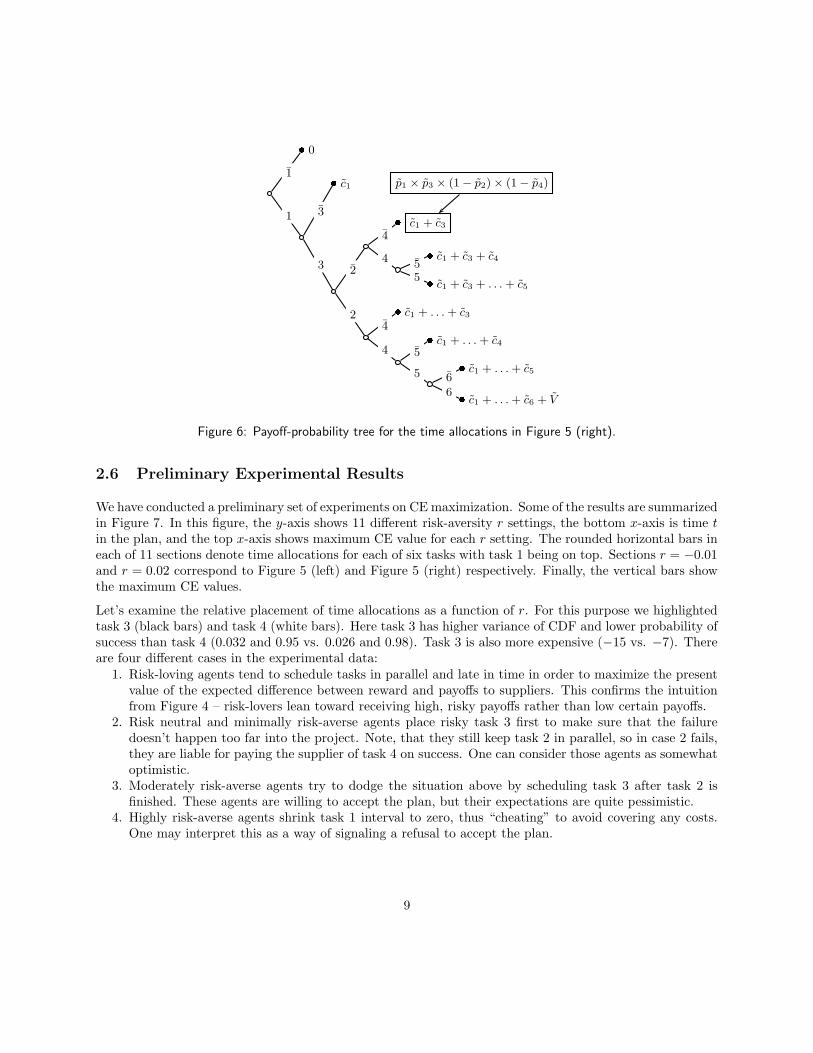
In the first call, the algorithm receives a “todo” task list T = N and a “done” task list D = ∅. All thesubsequent calls are recursive. To illustrate the idea behind this algorithm, we refer to the payoff-probabilitytree in Figure 6. This tree was built for the time allocations in Figure 5 (right) and reflects the precursorrelations for this case.

Looking at the time allocation, we note that with probability 1 − p1 task 1 fails, the customer agent doesnot pay or receive anything and stops the execution (path 1 in the tree). With probability pc

1 = p1 the agentproceeds with task 3 (path 1 in the tree). In turn, task 3 either fails with probability p1 × (1− p3), in whichcase the agent ends up stopping the plan and paying a total of c1 (path 1 → 3), or it is completed with thecorresponding probability pc

3 = p1 × p3. In the case where both 1 and 3 are completed, the agent starts both2 and 4 in parallel and becomes liable for paying c2 and c4 respectively even if the other task fails (paths1 → 3 → 2 → 4 and 1 → 3 → 2 → 4). If both 2 and 4 fail, the resulting path in the tree is 1 → 3 → 2 → 4and the corresponding payoff-probability pair is framed in the figure.

The algorithm’s complexity is O(

2K−1 × N)

, where K is the maximum number of tasks that are scheduledto be executed in parallel. Reducing the complexity of calcGamble is critical, since it is in the inner loopof the CE maximization process. In commercial projects the ratio K/N is likely to be low, since not many ofthese exhibit a high degree of parallelism. Our preliminary experiments allow us to conclude that the K/Nratio is lower for risk-averse agents (presumably, businessmen) than for risk-lovers (gamblers). These twoconsiderations may reduce the need for a faster algorithm, though additional work to improve the algorithmis planned.

8

�0

1

1

�c1

3

p1 × p3 × (1 − p2) × (1 − p4)

3 2

�c1 + c3

4

4�

c1 + c3 + c45

�c1 + c3 + . . . + c5

5

2�

c1 + . . . + c3

4

4

�c1 + . . . + c4

5

5�

c1 + . . . + c5

6

�c1 + . . . + c6 + V

6

Figure 6: Payoff-probability tree for the time allocations in Figure 5 (right).

2.6 Preliminary Experimental Results

We have conducted a preliminary set of experiments on CE maximization. Some of the results are summarizedin Figure 7. In this figure, the y-axis shows 11 different risk-aversity r settings, the bottom x-axis is time tin the plan, and the top x-axis shows maximum CE value for each r setting. The rounded horizontal bars ineach of 11 sections denote time allocations for each of six tasks with task 1 being on top. Sections r = −0.01and r = 0.02 correspond to Figure 5 (left) and Figure 5 (right) respectively. Finally, the vertical bars showthe maximum CE values.

Let’s examine the relative placement of time allocations as a function of r. For this purpose we highlightedtask 3 (black bars) and task 4 (white bars). Here task 3 has higher variance of CDF and lower probability ofsuccess than task 4 (0.032 and 0.95 vs. 0.026 and 0.98). Task 3 is also more expensive (−15 vs. −7). Thereare four different cases in the experimental data:

1. Risk-loving agents tend to schedule tasks in parallel and late in time in order to maximize the presentvalue of the expected difference between reward and payoffs to suppliers. This confirms the intuitionfrom Figure 4 – risk-lovers lean toward receiving high, risky payoffs rather than low certain payoffs.

2. Risk neutral and minimally risk-averse agents place risky task 3 first to make sure that the failuredoesn’t happen too far into the project. Note, that they still keep task 2 in parallel, so in case 2 fails,they are liable for paying the supplier of task 4 on success. One can consider those agents as somewhatoptimistic.

3. Moderately risk-averse agents try to dodge the situation above by scheduling task 3 after task 2 isfinished. These agents are willing to accept the plan, but their expectations are quite pessimistic.

4. Highly risk-averse agents shrink task 1 interval to zero, thus “cheating” to avoid covering any costs.One may interpret this as a way of signaling a refusal to accept the plan.

9

0 50 100 150

−0.03

−0.02

−0.01

0

0.01

0.02

0.03

0.04

0.05

0.06

0.07

0 1 2 3 4 5 6 7 8 9 10

−0.03

−0.02

−0.01

0

0.01

0.02

0.03

0.04

0.05

0.06

0.07CE

t

r

Figure 7: CE maximizing schedules and CE values for the plan in Figure 2 and r ∈ [−0.03, 0.07].

2.7 RFQ generation

In the previous section we have shown a way of generating a CE maximizing schedule of task execution,which we hereafter refer as the ideal schedule. The ideal schedule insures the highest possible quality ofthe bids that satisfy it, where by quality we assume some function of the expectations over the cost, theprobability of successful completion, and the profitability of the incoming bids in their feasible combinationswith other bids. At the same time it cannot serve as the optimal RFQ, since it is unlikely that bids will beavailable to cover precisely the same intervals as mandated by the CE maximizing schedule.

In order to construct a viable RFQ based on the CE maximizing schedule, the customer agent should lowerits expectations of the bid quality to some level by widening the RFQ time windows around the ideal ones,thus increasing4 the expected number of the incoming bids. In this section we discuss criteria that allow usto rationalize the selection among all such RFQs.

4At least to some extent, — there is a fair chance that the number of the incoming bids will cease to increase whenever RFQ

time windows become too large to inspire confidence on the part of suppliers.

10

We approach the optimal RFQ generation based on the ideal schedule as follows:

1. Measure the sensitivity of the expected bid quality to the deviations from the CE maximizing schedule.

2. Derive the relation between the quality of incoming bids and the size of RFQ time windows.

3. Decide on the choice of the optimal quality-quantity combination.

Note, the term “optimality” as we apply it to the choice of the customer agent can be expressed in other wordsas “individually rational and comprehensible.” That is, we search for the solution concept that generatesviable RFQs and is legible enough for a human user of the system.

2.7.1 CE sensitivity to schedule changes

We propose measuring the sensitivity of CE by investigating how CE values change with variations of a singletask n start time tsn in the ideal schedule. For the sake of brevity the resulting dependency of CE valuesis denoted by CE (tsn). Figure 8 shows CE (tsn) , n = 1 . . . 6 for our 6-task sample problem for r = −0.01and r = 0.02 respectively. In the figure y-axis of each horizontal stripe n represents the percentage ofthe maximum CE value, x-axis represents tsn and the horizontal lines with circle and cross ends show thecorresponding ideal schedules.

0 2 4 6 8 10

1

2

3

4

5

6t

#

0 2 4 6 8 10

1

2

3

4

5

6t

#

Figure 8: CE (tsn) graphs for the corresponding ideal schedules in Figure 5.

The tasks 1, 3 and 5 in the right graph are relatively restrictive to the start times of the bids that can bebundled with the ideal bids without considerably impairing the resulting bundle’s value. However, the factthat the task 2 in the right graph is more flexible does not guarantee that it will attract a higher numberof bids, since the latter depends both on the size of the corresponding time window and on the marketproperties of the task: resource availability, number of prospective bidders, seasonal changes, etc.

We assert that for the purpose of creating an optimal RFQ it is admissible to choose time windows basedon the sensitivity of CE to deviations of a single time restriction from the ideal schedule. The rationaleis that the relations between tasks are already encapsulated in the calculations of CE, so the change of

11

one restriction will approximate the rescheduling of several related tasks in the neighborhood of the idealschedule.

2.7.2 Quality vs. quantity

Observe, that the time window for the task n, {tsn|CE (tsn) ≥ x}, grows as the lowest expected CE value, x,decreases. The relation between these two variables for the tasks 3 and 4 of the test problem is shown inFigure 9. The corresponding relation between the lowest expected CE value and the expected number ofbids as a function of the window size is shown in Figure 10. In the last graph we assumed, for the sake ofexample, that the supply of the task 3 is higher than of the task 4, hence the difference in relative positionsof task 3 and task 4 graphs in the two figures.

0 1 2 3 40

20

40

60

80

100

t

% of max CE

task 3task 4

0 1 2 3 4 5 60

20

40

60

80

100

E#

% of max CE

task 3task 4

Figure 9: Relationship between the RFQ window size(shown in units of time on x-axis) and the lowest ad-missible percentage of the maximum CE value.

Figure 10: Relationship between the expected numberof bids (shown on x-axis) and the lowest admissible per-centage of the maximum CE value.

The type of graph in Figure 10 reflects the relation between the quality and the quantity of bids we weresearching for. Indeed, the only independent variable in this graph is tsn. The quantity of bids depends on thesize and positions of RFQ time windows that, in turn, depend on the decision about the lowest admissibleCE value. The quality of bids is a function of the RFQ choice and the properties of the plan. Finally, it isexpected that the customer agent will prefer a point on the graph to any point below and to the left of it,hence the optimal choice should lie on the graph.

2.7.3 Optimal quality-quantity choice and RFQ

We illustrate the decision process of the customer agent in Figure 11, where the customer agent’s preferencesover quality-quantity combinations are represented by a family of indifference curves and the graph of under-lying quality-quantity relationship derived in the text above5. Each indifference curve shows quality-quantity

5The precise derivation of the solution requires introduction of several concepts from economic theory that span beyond the

scope of this paper.

12

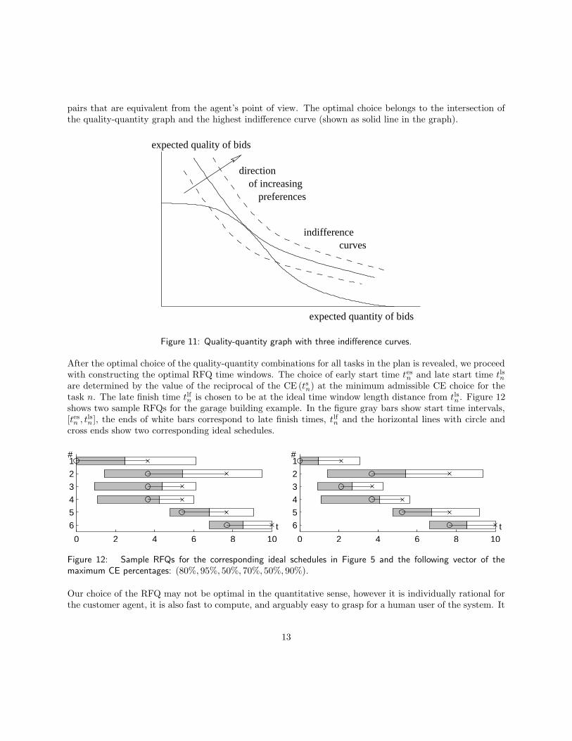
pairs that are equivalent from the agent’s point of view. The optimal choice belongs to the intersection ofthe quality-quantity graph and the highest indifference curve (shown as solid line in the graph).

direction

expected quality of bids

expected quantity of bids

curvesindifference

preferencesof increasing

Figure 11: Quality-quantity graph with three indifference curves.

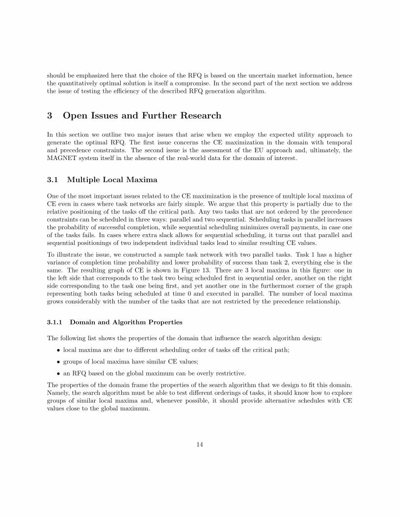
After the optimal choice of the quality-quantity combinations for all tasks in the plan is revealed, we proceedwith constructing the optimal RFQ time windows. The choice of early start time tesn and late start time tlsnare determined by the value of the reciprocal of the CE (tsn) at the minimum admissible CE choice for thetask n. The late finish time tlfn is chosen to be at the ideal time window length distance from tlsn . Figure 12shows two sample RFQs for the garage building example. In the figure gray bars show start time intervals,[tesn , tlsn ], the ends of white bars correspond to late finish times, tlfn and the horizontal lines with circle andcross ends show two corresponding ideal schedules.

0 2 4 6 8 10

1

2

3

4

5

6 t

#

0 2 4 6 8 10

1

2

3

4

5

6 t

#

Figure 12: Sample RFQs for the corresponding ideal schedules in Figure 5 and the following vector of themaximum CE percentages: (80%, 95%, 50%, 70%, 50%, 90%).

Our choice of the RFQ may not be optimal in the quantitative sense, however it is individually rational forthe customer agent, it is also fast to compute, and arguably easy to grasp for a human user of the system. It

13

should be emphasized here that the choice of the RFQ is based on the uncertain market information, hencethe quantitatively optimal solution is itself a compromise. In the second part of the next section we addressthe issue of testing the efficiency of the described RFQ generation algorithm.

3 Open Issues and Further Research

In this section we outline two major issues that arise when we employ the expected utility approach togenerate the optimal RFQ. The first issue concerns the CE maximization in the domain with temporaland precedence constraints. The second issue is the assessment of the EU approach and, ultimately, theMAGNET system itself in the absence of the real-world data for the domain of interest.

3.1 Multiple Local Maxima

One of the most important issues related to the CE maximization is the presence of multiple local maxima ofCE even in cases where task networks are fairly simple. We argue that this property is partially due to therelative positioning of the tasks off the critical path. Any two tasks that are not ordered by the precedenceconstraints can be scheduled in three ways: parallel and two sequential. Scheduling tasks in parallel increasesthe probability of successful completion, while sequential scheduling minimizes overall payments, in case oneof the tasks fails. In cases where extra slack allows for sequential scheduling, it turns out that parallel andsequential positionings of two independent individual tasks lead to similar resulting CE values.

To illustrate the issue, we constructed a sample task network with two parallel tasks. Task 1 has a highervariance of completion time probability and lower probability of success than task 2, everything else is thesame. The resulting graph of CE is shown in Figure 13. There are 3 local maxima in this figure: one inthe left side that corresponds to the task two being scheduled first in sequential order, another on the rightside corresponding to the task one being first, and yet another one in the furthermost corner of the graphrepresenting both tasks being scheduled at time 0 and executed in parallel. The number of local maximagrows considerably with the number of the tasks that are not restricted by the precedence relationship.

3.1.1 Domain and Algorithm Properties

The following list shows the properties of the domain that influence the search algorithm design:

• local maxima are due to different scheduling order of tasks off the critical path;

• groups of local maxima have similar CE values;

• an RFQ based on the global maximum can be overly restrictive.

The properties of the domain frame the properties of the search algorithm that we design to fit this domain.Namely, the search algorithm must be able to test different orderings of tasks, it should know how to exploregroups of similar local maxima and, whenever possible, it should provide alternative schedules with CEvalues close to the global maximum.

14

0

5

10

0

5

10

0

5

10

15

20

task 1 start timetask 2 start time

CE

Figure 13: Local maxima for two parallel tasks.

We propose a search algorithm based on the ideas of the Simulated Annealing [27] and Genetic Algorithms [7].The algorithm will combine the stochastic temperature-driven nature of the Simulated Annealing with thesimultaneous search space exploration of the Genetic Algorithms. In this section we describe the proposedalgorithm in more details and explain the rationale of its design.

3.1.2 Search Algorithm

The proposed search algorithm explores several alternative schedules in parallel. The initial set of alterna-tives can be generated in many ways: random generation, hill-climbing from random schedule, CPM, etc.The execution of the algorithm proceeds in steps by randomly applying one of the following five transfor-mation rules to each alternative schedule. Figure 14 illustrates the algorithm for the case of three pairwiseindependent tasks.

Distortion is performed with the highest probability. Distortion alters start and finish times of one orseveral tasks as well as adjusts time windows of all related tasks to maintain precedence constraints(1 → 5 → 9 in Figure 14). Distortion mimics the basic step of the SA algorithm.

Shuffling is performed with lower probability than the distortion, yet with the higher probability than therest of the transformations. Shuffling changes relative scheduling of two or more tasks wherever itis permitted by the precedence constraints. Shuffling can switch ordering of tasks (6 → 10), changesequential ordering to parallel or reschedule parallel tasks to be executed sequentially (4 → 8). Themajor role of shuffling is to explore local maxima that have similar CE values due to different schedulingof tasks off the critical path.

Explosion adds a copy of the subject schedule to the list of alternatives (2 → 6, 7). Explosion complimentsshuffling by allowing for simultaneous exploration of the groups of similar schedules. We may chooseto decrease the rate of explosions with the annealing temperature to focus on improving the currentset of solution after the search space was explored to extent.

15

R

D

E

S

D

S

I

I 11

1

2

3

4

5

6

7

8

9

10

Figure 14: Two steps of the search algorithm execution.

Implosion merges two similar6 schedules in one. Implosion helps reducing computational expenses fromcrowding several alternative schedules around one maximum (7, 8 → 11). The rate of implosions willchange in the opposite direction to the rate of explosions.

Removal eliminates alternatives that do not score well relative to others (3 → ∅). This transformationtakes care of the schedules that are stuck in local maxima with low CE values. The rate of removalsgrows as the annealing temperature decreases.

Each of the first four transformation is tested against SA temperature rule whenever it leads to a decreasein the CE value. In case it is discarded, other transformations are chosen at random and applied until oneof them increases CE or passes the temperature rule.

The probabilities of transformations as well as details of the proposed search algorithm’s properties aresubject to further research. It is reasonable to believe though that the comprehensive study of the RFQgeneration mechanism is only possible in the dynamic market environment. In the next section we discussthe approach to the large-scale testing of the MAGNET system that will provide us with the necessary data.

3.2 Evolutionary Framework for Large-scale Testing

After finalizing the EU-based customer agent, as well as developing its supplier counterpart, we plan todevote efforts to testing them against various criteria. In particular, we are interested in testing how wellindividual agents interact in a populated market. This will help us understand the nuances of the applicationof EU to RFQ generation. The major goals of this part of the study would be:

• provide the statistical data necessary for the evaluation of the theoretical assumptions and derivations;

• facilitate the understanding of the nuances of the EU-based RFQ generation and to drive improvementsto the theory and implementation;

6Similarity is a function the distance between two schedules as between two points in the 2N-dimensional time space.

16

• study the relative performance of agents in the simulated market, developing an understanding of theproperties of automated and mixed-initiative combinatorial auction-based trading societies.

The most compelling approach would be to gather a rich set of statistical data from a commerce domain.That has not proven to be feasible, for two reasons. First, few industrial organizations are sufficiently opento expose the type of data you would need to do that, and we would need data from multiple organizationsin a single market. Second, data is gathered to serve a purpose, and our experience tells us that when youattempt to apply existing data to a new purpose, it frequently turns out to be full of inconsistencies andmethodological problems.

In lieu of using real industry data, we will design our large-scale test suite atop an abstract domain withcontrollable statistics, and an evolutionary approach to economic simulation. The structure of the simulationwill be defined like this:

• The society will initially consist of one customer agent and many heterogeneous supplier agents. Thechoice of this setup is due to the assumption that there is little competition on the customer side, socustomers can be replaced by one representative agent who issues RFQs with high frequency. Eachsupplier will initially be provided with a “factory” that produces one type of good or service andmaintains the schedule of production.

• The customer agent will issue RFQs for one or several tasks according to a (stationary or not) Poissonprocess. Multiple RFQs will be open concurrently, so that suppliers must frequently evaluate severalRFQs at once. Upon receiving bids, the customer agent will find the winning bundle of bids and awardbids. After that, it will monitor the execution of the plan and make appropriate payments to suppliers.

• The performance of supplier agents will be evaluated on the basis of profit averaged over a substantialperiod of time. The market will run in an evolutionary fashion, i.e. by removing suppliers with negativeprofits over periods of time, and introducing new suppliers with strategies from the pool of all availablestrategies whenever the average profit in the market exceeds some positive value.

• The information on successful bids and completed tasks will be collected, processed, and provided tothe customer agent to be used in the RFQ generation and winner determination procedures.

The rationale behind our choice of an evolutionary framework is that it provides the necessary informationwithout requiring any complex theory on agent motivation, optimization criteria, or strategic interaction.Unsuccessful species of supplier agents will be washed away from the market, creating places for the more fit.At the same time, the market will provide customer agents with dynamic information on supplier availability,market prices, and cumulative success probabilities.

Evolutionary frameworks have been used extensively in Economics [21, 29, 38]. The framework will allow usto tune the market by tweaking the frequency of issuing RFQs and will allow for the dynamic introduction ofnew supplier strategies, without imposing any assumptions on the nature of strategies. We will later extendthe framework to support trade games to be played with human subjects. This will be a tool specially usefulfor teaching, as a tool to explore strategic behaviors and to study the emergence of cooperation [1, 2].

17

4 Related Work

Expected Utility Theory [26] is a mature field of Economics that has attracted many supportive as well ascritical studies, both theoretical [17, 18] and empirical [14, 36]. We believe that expected utility will playan increasing role in automated auctions, since it provides a practical way of describing risk estimations andtemporal preferences.

Our long term objective is to automate the scheduling/execution cycle of an autonomous agent that needsthe services of other agents to accomplish its tasks. Pollack’s DIPART system [25] and SharedPlans [11]assume multiple agents that operate independently but all work towards the achievement of a global goal.Our agents are trying to achieve their own goals and to maximize their profits; there is no global goal.

Combinatorial auctions are becoming an important mechanism not just for agent-mediated electronic com-merce [12, 41, 32] but also for allocation of tasks to cooperative agents (see, for instance, [13, 6]).

In [13] combinatorial auctions are used for the initial commitment decision problem, which is the probleman agent has to solve when deciding whether to join a proposed collaboration. Their agents have precedenceand hard temporal constraints. However, to reduce search effort, they use domain-specific roles, a shorthandnotation for collections of tasks. In their formulation, each task type can be associated with only a single role.MAGNET agents are self-interested, and there are no limits to the types of tasks they can decide to do. In [9]scheduling decisions are made not by the agents, but instead by a central authority. The central authorityhas insight to the states and schedules of participating agents, and agents rely on the authority for supportingtheir decisions. Nisan’s bidding language [23] allows bidders to express certain types of constraints, but inMAGNET both the bidder and the bid-taker (the customer) need to communicate constraints.

Despite the abundance of work in auctions [20], limited attention has been devoted to auctions over taskswith complex time constraints and interdependencies. In [24], a method is proposed to auction a sharedtrack line for train scheduling. The problem is formulated with mixed integer programming, with manydomain-specific optimizations. Bids are expressed by specifying a price to enter a line and a time window.The bidding language, which is similar to what we use in MAGNET, avoids use of discrete time slots. Timeslots are used in [40], where a protocol for decentralized scheduling is proposed. The study is limited toscheduling a single resource. MAGNET agents deal with multiple resources.

Most work in supply-chain management is limited to hierarchical modeling of the decision making process,which is inadequate for distributed supply-chains, where each organization is self-interested, not cooperative.Walsh et al [39] propose a protocol for combinatorial auctions for supply chain formation, using a game-theoretical perspective. They allow complex task networks, but do not include time constraints. MAGNETagents have also to ensure the scheduling feasibility of the bids they accept, and must evaluate risk as well.Agents in MASCOT [31] coordinate scheduling with the user, but there is no explicit notion of payments orcontracts, and the criteria for accepting/rejecting a bid are not explicitly stated. Their major objective is toshow policies that optimize schedules locally [15]. Our objective is to optimize the customer’s utility.

In MAGNET agents interact with each other through a market. The market infrastructure provides acommon vocabulary, collects statistical information that helps agents estimate costs, schedules, and risks,and acts as a trusted intermediary during the negotiation process. The market acts also as a matchmaker [37],allowing us to ignore the issue of how agents will find each other.

The determination of winners of combinatorial auctions [30] is hard. Dynamic programming [30] works well

18

for small sets of bids, but does not scale and imposes significant restrictions on the bids. Algorithms suchas CABOB [34], Bidtree [33] and CASS [8] reduce the search complexity. Reeves et al [28] use auctionmechanisms to ”fill in the blanks” in prototype declarative contracts that are specified in a language basedon Courteous Logic Programming [10]. These auctions support bidding on many attributes other than price,but the problem of combining combinatorial bids with side constraints is not addressed.

Leyton-Brown et al [16] suggest a way of constructing a universal test suite for winner determination algo-rithms in combinatorial auctions. Their work does not include cases with precedence and time constraintsand, thus, is not directly applicable to the MAGNET framework. It nevertheless provides well-understoodtest cases for comparing the performance of algorithms.

5 Conclusions

Auction mechanisms are an effective approach to negotiation among groups of self-interested economic agents.We are particularly interested in situations where agents need to negotiate over multiple factors, includingnot only price, but task combinations and temporal factors as well.

We have shown how an agent can use information about the risk posture of its principal, along with marketstatistics, to formulate Requests for Quotes that optimize the tradeoff between risk and value, and increasethe quality of the bids received. This requires deciding how to sequence tasks and how much time to allocateto each of them. Bids closest to the specified time windows are the most preferred risk-payoff combinations.

The work described here is a part of a larger effort at the University of Minnesota that aims to learn howautonomous or semi-autonomous agents can be used in complex commerce-oriented domains.

Acknowledgments

Partial support for this research is gratefully acknowledged from the National Science Foundation underaward NSF/IIS-0084202.

References

[1] R. M. Axelrod. The evolution of cooperation. Basic Books, 1984.

[2] Robert Axelrod. The complexity of cooperation. Princeton University Press, 1997.

[3] John Collins, Corey Bilot, Maria Gini, and Bamshad Mobasher. Decision processes in agent-basedautomated contracting. IEEE Internet Computing, pages 61–72, March 2001.

[4] John Collins, Maria Gini, and Bamshad Mobasher. Multi-agent negotiation using combinatorial auc-tions with precedence constraints. Technical Report 02-009, University of Minnesota, Department ofComputer Science and Engineering, Minneapolis, Minnesota, February 2002.

19

[5] John Collins, Maksim Tsvetovat, Rashmi Sundareswara, Joshua Van Tonder, Maria Gini, and BamshadMobasher. Evaluating risk: Flexibility and feasibility in multi-agent contracting. In Proc. of the ThirdInt’l Conf. on Autonomous Agents, May 1999.

[6] M. B. Dias and A. Stentz. A free market architecture for distributed control of a multirobot system. InSixth Int’l Conf. on Intelligent Autonomous Systems, pages 115–122, Venice, Italy, July 2000.

[7] Stephanie Forrest. Genetic algorithms: Principles of natural selection applied to computation. Science,261:872–878, 1993.

[8] Yuzo Fujishima, Kevin Leyton-Brown, and Yoav Shoham. Taming the computational complexity ofcombinatorial auctions: Optimal and approximate approaches. In Proc. of the 16th Joint Conf. onArtificial Intelligence, 1999.

[9] Alyssa Glass and Barbara J. Grosz. Socially conscious decision-making. In Proc. of the Fourth Int’lConf. on Autonomous Agents, pages 217–224, June 2000.

[10] B. N. Grosof, Y. Labrou, and H. Y. Chan. A declarative approach to business rules in contracts:Courteous logic programs in XML. In Proc. of ACM Conf on Electronic Commerce (EC’99), pages68–77. ACM, 1999.

[11] Barbara J. Grosz, Luke Hunsberger, and Sarit Kraus. Planning and acting together. AI Magazine,20(4):23–34, 1999.

[12] Robert H. Guttman, Alexandros G. Moukas, and Pattie Maes. Agent-mediated electronic commerce: asurvey. Knowledge Engineering Review, 13(2):143–152, June 1998.

[13] Luke Hunsberger and Barbara J. Grosz. A combinatorial auction for collaborative planning. In Proc.of 4th Int’l Conf on Multi-Agent Systems, pages 151–158, Boston, MA, 2000. IEEE Computer SocietyPress.

[14] Bruno Jullien and Bernard Salanie. Estimating preferences under risk: The case of racetrack bettors.The Journal of Political Economy, 108(3):503–530, June 2000.

[15] Dag Kjenstad. Coordinated Supply Chain Scheduling. PhD thesis, Dept of Production and QualityEngineering, Norvegian University of Science and Technology, Trondheim, Norway, 1998.

[16] Kevin Leyton-Brown, Mark Pearson, and Yoav Shoham. Towards a universal test suite for combinatorialauction algorithms. In Proc. of ACM Conf on Electronic Commerce (EC’00), pages 66–76, Minneapolis,MN, October 2000.

[17] Mark J. Machina. Choice under uncertainty: Problems solved and unsolved. The Journal of EconomicPerspectives, 1(1):121–154, 1987.

[18] Mark J. Machina. Dynamic consistency and non-expected utility models of choice und er uncertainty.The Journal of Economic Literature, 27(4):1622–1668, December 1989.

[19] Andreu Mas-Colell, Michael D. Whinston, and Jerry R. Green. Microeconomic Theory. Oxford Univer-sity Press, January 1995.

[20] R. McAfee and P. J. McMillan. Auctions and bidding. Journal of Economic Literature, 25:699–738,1987.

20

[21] Richard R. Nelson. Recent evolutionary theorizing about economic change. Journal of EconomicLiterature, 33(1):48–90, March 1995.

[22] Noam Nisan. Bidding and allocation in combinatorial auctions. In 1999 NWU Microeconomics Work-shop, 1999.

[23] Noam Nisan. Bidding and allocation in combinatorial auctions. In Proc. of ACM Conf on ElectronicCommerce (EC’00), pages 1–12, Minneapolis, Minnesota, October 2000. ACM SIGecom, ACM Press.

[24] David C. Parkes and Lyle H. Ungar. An auction-based method for decentralized train scheduling. InProc. of the Fifth Int’l Conf. on Autonomous Agents, pages 43–50, Montreal, Quebec, May 2001. ACMPress.

[25] Martha E. Pollack. Planning in dynamic environments: The DIPART system. In A. Tate, editor,Advanced Planning Technology. AAAI Press, 1996.

[26] John W. Pratt. Risk aversion in the small and in the large. Econometrica, 32:122–136, 1964.

[27] Colin R. Reeves. Modern Heuristic Techniques for Combinatorial Problems. John Wiley & Sons, NewYork, NY, 1993.

[28] Daniel M. Reeves, Michael P. Wellman, and Benjamin N. Grosof. Automated negotiation from declar-ative contract descriptions. In Proc. of the Fifth Int’l Conf. on Autonomous Agents, pages 51–58,Montreal, Quebec, May 2001. ACM Press.

[29] David Rode. Market efficiency, decision processes, and evolutionary games. Department of Social andDecision Sciences, Carnegie Mellon University, March 1997.

[30] Michael H. Rothkopf, Alexander Pekec, and Ronald M. Harstad. Computationally manageable combi-natorial auctions. Management Science, 44(8):1131–1147, 1998.

[31] Norman M. Sadeh, David W. Hildum, Dag Kjenstad, and Allen Tseng. MASCOT: an agent-basedarchitecture for coordinated mixed-initiative supply chain planning and scheduling. In Workshop onAgent-Based Decision Support in Managing the Internet-Enabled Supply-Chain, at Agents ’99, pages133–138, May 1999.

[32] Tuomas Sandholm. An algorithm for winner determination in combinatorial auctions. In Proc. of the16th Joint Conf. on Artificial Intelligence, pages 524–547, 1999.

[33] Tuomas Sandholm. Approaches to winner determination in combinatorial auctions. Decision SupportSystems, 28(1-2):165–176, 2000.

[34] Tuomas Sandholm, Subhash Suri, Andrew Gilpin, and David Levine. CABOB: A fast optimal algorithmfor combinatorial auctions. In Proc. of the 17th Joint Conf. on Artificial Intelligence, Seattle, WA, USA,August 2001.

[35] Tuomas W. Sandholm. Negotiation Among Self-Interested Computationally Limited Agents. PhD thesis,Department of Computer Science, University of Massachusetts at Amherst, 1996.

[36] V. Kerry Smith and William H. Desvousges. An empirical analysis of the economic value of risk changes.The Journal of Political Economy, 95(1):89–114, February 1987.

21

[37] Katia Sycara, Keith Decker, and Mike Williamson. Middle-agents for the Internet. In Proc. of the 15thJoint Conf. on Artificial Intelligence, pages 578–583, 1997.

[38] Leigh Tesfatsion. Agent-based computational economics: Growing economies from the bottom up. ISUEconomics Working Paper No. 1, Department of Economics, Iowa State University, December 2001.

[39] William E. Walsh, Michael Wellman, and Fredrik Ygge. Combinatorial auctions for supply chain for-mation. In Proc. of ACM Conf on Electronic Commerce (EC’00), October 2000.

[40] Michael P. Wellman, William E. Walsh, Peter R. Wurman, and Jeffrey K. MacKie-Mason. Auctionprotocols for decentralized scheduling. Games and Economic Behavior, 35:271–303, 2001.

[41] Peter R. Wurman, Michael P. Wellman, and William E. Walsh. The Michigan Internet AuctionBot:A configurable auction server for human and software agents. In Second Int’l Conf. on AutonomousAgents, pages 301–308, May 1998.

22