asdxa

ADAPTIVE FILTERS IInstructor :Dr Aamer Iqbal Bhatti

ADAPTIVE FILTERS IInstructor :Dr. Aamer Iqbal BhattiRandom Variable and Stochastic Random Variable and Stochastic

ProcessesProcessesProcessesProcesses

Lecture# Lecture# 0202

June 3, 2003 Lecture 2 1

Optimal Filters

Word optimal means doing a job in the best possible way.p g j p y Before beginning search for such an optimal solution , the

job must be defined. A mathematical scale must be established for what best

means , and the possible alternatives must be spelled out. Unless there is agreement an these qualifiers a claim that a

system is optimal is really meaningless.

3 June 2003Lecture 22

Statement for the Optimal ProblemA mathematical statement of optimalproblem consists ofproblem consists of Description of system constraints and possible

alternativesalternatives A description of task to be performed A statement of the criterion for judging optimal A statement of the criterion for judging optimal

performance


Linear Optimal Filtering: Statement of the Problem

Output of the system is used to provide an estimate of the desired responsep

Filter input and output represents single realization of respective stochastic processes i.e. the process to be p p pfiltered and the desired process after filtering of the input process.


Linear Optimal Filtering: Statement of the Problem Estimation is accomplished by an reducing an error with Estimation is accomplished by an reducing an error with

the statistical characteristics of its own. Mathematical scale for the performance of the filtering Mathematical scale for the performance of the filtering

system is to minimize the estimation error produced by the filter approximationsthe filter approximations


Linear Optimal Filtering: Statement of the blProblem

Constraints which have been placed on the system are p y The system is linear , which makes the problem

mathematically easy to tracty y The filter operates in discrete time


Choice of the Filter Parameters Choice for the finite or infinite impulse response of the

filter depends on the practical considerationsp p Selection of the statistical criterion for optimization of

filter is influenced by mathematical tractabilityy y


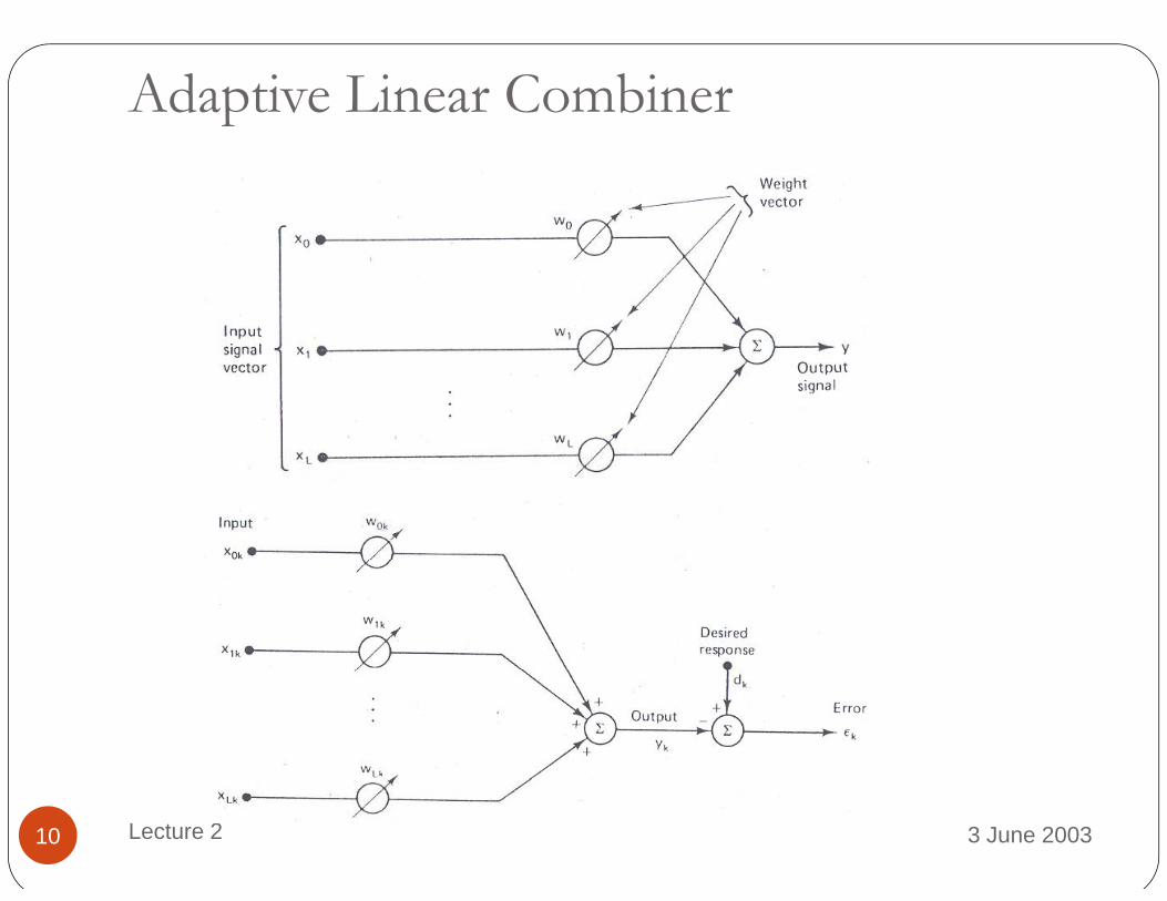
Adaptive Linear Combiner Adaptive Linear Combiner appears in most of adaptive

systemsy It is the single most important element in learning

systemsy It is a non-recursive digital filter and its performance is

quite simpleq p Linear adaptive consists of a multiple summer and their

associated weightsg


Adaptive Linear Combiner These weights are varied in order to change the response

of the system to achieve some desired response Procedure for adapting weights is called “Weight

Adjustment” Adaptive linear combiner is a linear system once its

weights are adjustedD i i h dj i h f i f h During weight adjustment weights are function of the input vector


Adaptive Linear Combinerp


Input Signal and Weight Vectors

There are two types of inputsSimultaneous inputs from different sourcesSequential Samples or single input

Input vector for both of them is are given byp g y

T

TLk1k0k

I tSi l

xxx :Inputs Multiple

L-k1-kk xxx:Input Single


Input Signal and Weight Vectors

First of these is for the spatial domain and second one is for ptemporal domain

Response for spatial and temporal inputs are given byp p p p g y

L

llklk xw

0ky:Input Single

L

lkllk

l

xw0

k

0

y:Input Multiple

kT

kkTk

l

XWWX

k

0

y :FormMatrix In




Figure


Figure


Figure


Random Variable and StatisticsRandom Variable The study of Probability

d R d V i bl i

Statistics On the other hand for the

study of statistics we dealand Random Variables is concerned with mathematical function of

study of statistics we deal with random data.

X=[1 -2 1 -4 4 ]mathematical function of PDF or CDF.

X [1, 2,1, 4,4,………..] We can compute Average

and Variance. N1

N

iix

NxE

1

1][

22 ])[(][][ xExExVar

In DSP and Communication we deal

])[(][][ xExExVar

)(xpx

We compute Mean and Variance from PDF

with data along with some supposition about its probability distribution

probability distribution

dxxxpxE x )(][ 22 ])[(][][ xExExVar

Pair of Random Variables We deal with joint PDF and joint

CDF to know the random behavior of pair of RV

Pair of random can be visualized by histogram or scatter plot.

k d bof pair of RV. We can compute Marginal and

Conditional PDF’s and CDF’s.

We can make an idea about their corelatedness and uncorrelatedness.

We can compute correlation and We can compute their marginal

means, variances, correlation and correlation coefficient

W pcorrelation coefficient.

11correlation coefficient.

Dependence and Independence. Correlation: How a random variable

is similar or dissimilar in its statistics

11 XYp p

How the chance of occurrence of one random variable effects the chance of occurrence of other

is similar or dissimilar in its statistics from other random variable.

chance of occurrence of other random variable

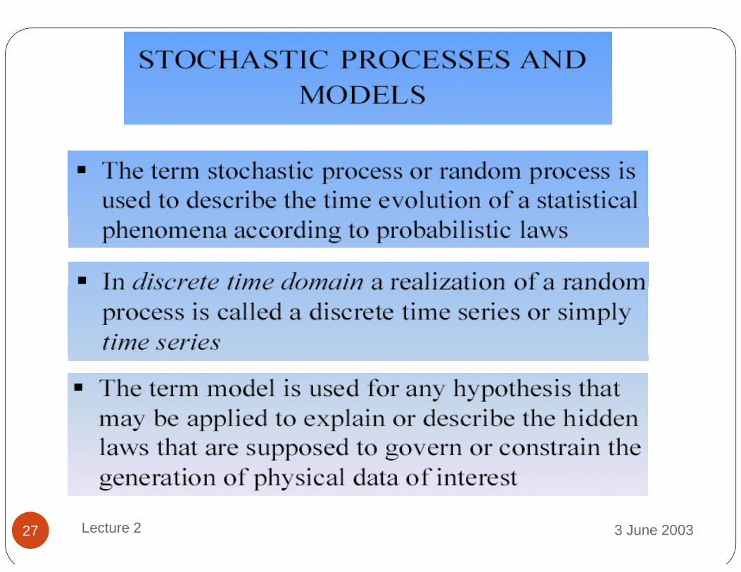
Stochastic or Random Processes Stochastic process (random process) is used to describe

the time evolution of a statistical phenomenon.the time evolution of a statistical phenomenon. Stochastic process is a representation of many or

infinite time series of random datainfinite time series of random data.

1 1 . 5

9 . 5

1 0

1 0 . 5

1 1

0 2 0 4 0 6 0 8 0 1 0 0 1 2 0 1 4 0 1 6 08

8 . 5

9

Stationary and Wide Sense Stationary A stochastic process is Strict Sense Stationary(SSS), if its

statistical properties are invariant to a time shiftp p Joint pdf of {x(n), x(n-1), ... , x(n-M)} remain the same

regardless of n. Joint pdf is not easy to obtain,

First and second moments are used frequently.

A stochastic process is Wide Sense Stationary(WSS), if its first and second order statistical properties are i i i hifinvariant to a time shift. Statistic expectation: mx(n)=E[x(n)] Autocorrelation function: For a stochastic process {x(n)} Autocorrelation function: For a stochastic process {x(n)}

φxx(n,m)=E[x(n)x*(m)]

Ergodic Processes Ensemble averages (expectations) are across the process -> can be obtained

analytically (actual expec.) Sample (time) averages are along the process > can be obtained emprically Sample (time) averages are along the process -> can be obtained emprically

(from realizations of a process) (estimated expectation)

1 1 .5

1 0

1 0 .5

1 1

sample (time)

8 5

9

9 .5

average

0 2 0 4 0 6 0 8 0 1 0 0 1 2 0 1 4 0 1 6 08

8 .5

Ensemble

If sample averages converge to ensemble averages in, e.g. mean square error sense,

average

We call the process x(n) as ergodic.

Correlation Function Auto Correlation Function φxx(n,m)=E[x(n)x*(m)];φxx( , ) [ ( ) ( )]; φxx(k)=E[x(n)x*(n-k)];

Properties of Auto Correlation Function.P ope t es o uto Co e at o Fu ct o . |φxx(k)|≤φxx(0) φxx(k)=φxx(-k)φxx( ) φxx( ) φxx(0)=E[x2(n)] x[n] has no periodic component.2

||ˆ)(lim xkxxk

[ ] p p

x[n] is argodic, zero mean.

||)(xxk

0)(lim||

kxxk [ ] g

|| k

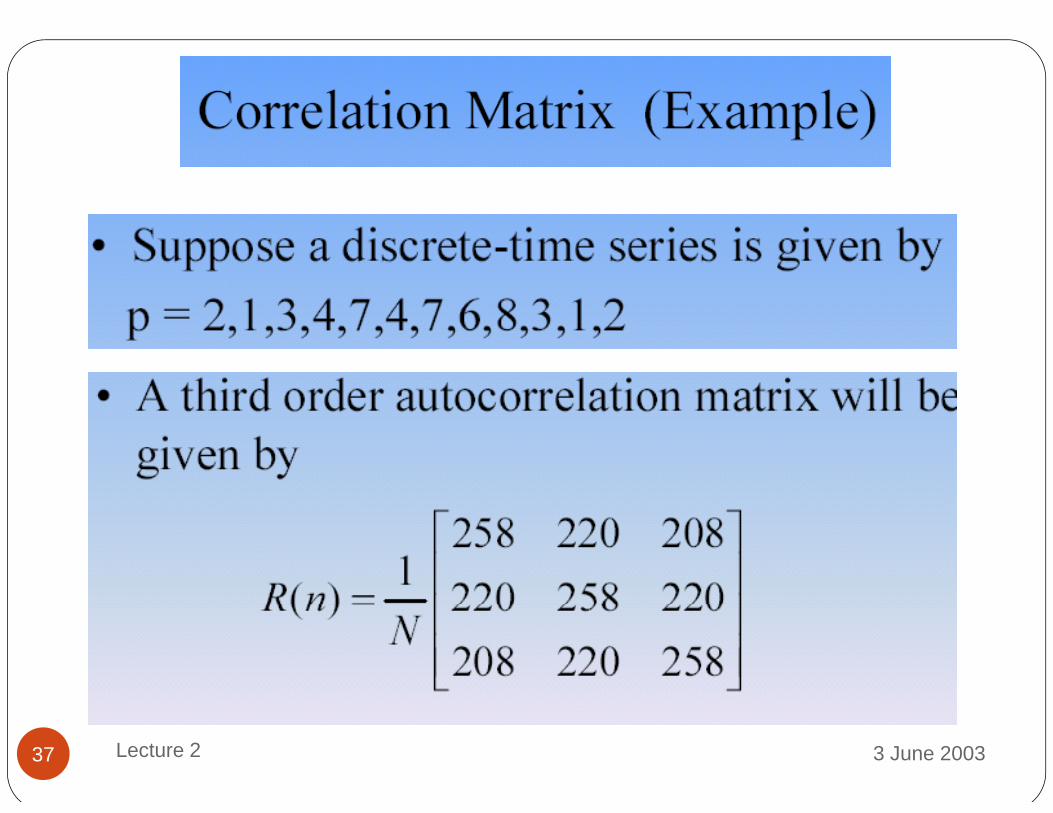
Correlation Matrix >> x=[1 -2 1 3];

>> XX=xcorr(x)

XX =

3 -5 -1 15 -1 -5 3

>> R=toeplitz(XX(4:end))

R =R

15 -1 -5 3

-1 15 -1 -5

-5 -1 15 -1

3 -5 -1 15 3 -5 -1 15

Auto Correlation Process Auto correlation of White Gaussian Noise. Auto correlation of slowly varying Process.Auto correlation of slowly varying Process. Auto correlation of rapidly varying process.

Properties of Auto Correlation Matrix Property 1: The correlation matrix of a stationary discrete-

time stochastic process is Hermitian symmetric. Property 2: The correlation matrix of a stationary discrete-

time stochastic process is Toeplitz. Property 3: The correlation matrix of a discrete time Property 3: The correlation matrix of a discrete-time

stochastic process is always non-negative definite and almost always positive definite.

Property 4: The correlation matrix of a w.s.s. process is nonsingular due to the unavoidable presence of additive noisenoise.

Property 5: If the order of the elements of the vector u(n) is (time)-reversed, the effect is the transposition of the ( ) , pautocorrelation matrix.


Equations


EquationsEquations



















Back


Back


Back


Back 1

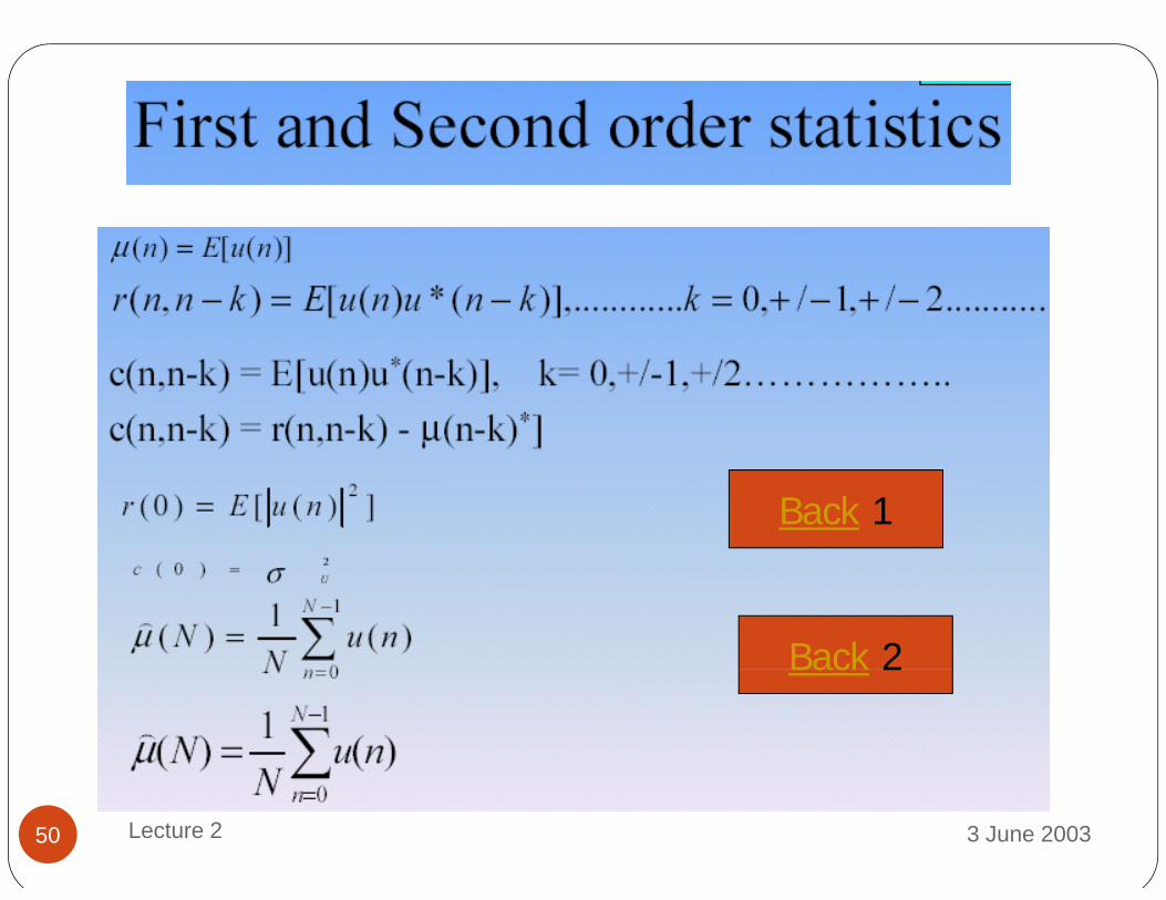
Back 2Back 2


Documents

asdxa