Embed Size (px)
Citation preview
This article was downloaded by: [New Jersey Institute of Technology]On: 28 February 2014, At: 08:46Publisher: Taylor & FrancisInforma Ltd Registered in England and Wales Registered Number: 1072954 Registered office: Mortimer House,37-41 Mortimer Street, London W1T 3JH, UK
Journal of the American Statistical AssociationPublication details, including instructions for authors and subscription information:http://amstat.tandfonline.com/loi/uasa20
Multiple Testing in a Two-Stage Adaptive Design WithCombination Tests Controlling FDRSanat K. Sarkar a , Jingjing Chen b & Wenge Guo ca Department of Statistics , Temple University , Philadelphia , PA , 19122b Clinical Statistics, MedImmune/ AstraZeneca , Gaithersburg , MD , 20878c Department of Mathematical Sciences , New Jersey Institute of Technology , Newark , NJ ,07102Accepted author version posted online: 24 Aug 2013.Published online: 19 Dec 2013.
To cite this article: Sanat K. Sarkar , Jingjing Chen & Wenge Guo (2013) Multiple Testing in a Two-Stage Adaptive DesignWith Combination Tests Controlling FDR, Journal of the American Statistical Association, 108:504, 1385-1401, DOI:10.1080/01621459.2013.835662
To link to this article: http://dx.doi.org/10.1080/01621459.2013.835662
PLEASE SCROLL DOWN FOR ARTICLE
Taylor & Francis makes every effort to ensure the accuracy of all the information (the “Content”) containedin the publications on our platform. However, Taylor & Francis, our agents, and our licensors make norepresentations or warranties whatsoever as to the accuracy, completeness, or suitability for any purpose of theContent. Any opinions and views expressed in this publication are the opinions and views of the authors, andare not the views of or endorsed by Taylor & Francis. The accuracy of the Content should not be relied upon andshould be independently verified with primary sources of information. Taylor and Francis shall not be liable forany losses, actions, claims, proceedings, demands, costs, expenses, damages, and other liabilities whatsoeveror howsoever caused arising directly or indirectly in connection with, in relation to or arising out of the use ofthe Content.
This article may be used for research, teaching, and private study purposes. Any substantial or systematicreproduction, redistribution, reselling, loan, sub-licensing, systematic supply, or distribution in anyform to anyone is expressly forbidden. Terms & Conditions of access and use can be found at http://amstat.tandfonline.com/page/terms-and-conditions

Supplementary materials for this article are available online. Please go to www.tandfonline.com/r/JASA
Multiple Testing in a Two-Stage Adaptive DesignWith Combination Tests Controlling FDR
Sanat K. SARKAR, Jingjing CHEN, and Wenge GUO
Testing multiple null hypotheses in two stages to decide which of these can be rejected or accepted at the first stage and which should befollowed up for further testing having had additional observations is of importance in many scientific studies. We develop two procedures,each with two different combination functions, Fisher’s and Simes’, to combine p-values from two stages, given prespecified boundaries onthe first-stage p-values in terms of the false discovery rate (FDR) and controlling the overall FDR at a desired level. The FDR control is provedwhen the pairs of first- and second-stage p-values are independent and those corresponding to the null hypotheses are identically distributedas a pair (p1, p2) satisfying the p-clud property. We did simulations to show that (1) our two-stage procedures can have significant powerimprovements over the first-stage Benjamini–Hochberg (BH) procedure compared to the improvement offered by the ideal BH procedurethat one would have used had the second stage data been available for all the hypotheses, and can continue to control the FDR under somedependence situations, and (2) can offer considerable cost savings compared to the ideal BH procedure. The procedures are illustratedthrough a real gene expression data. Supplementary materials for this article are available online.
KEY WORDS: Early acceptance and rejection boundaries; False discovery rate; Single-stage BH procedure; Stepdown test; Stepup test;Two-stage multiple testing.
1. INTRODUCTION
Gene association or expression studies that usually involve alarge number of endpoints (i.e., genetic markers) are often quiteexpensive. Such studies conducted in a multistage adaptivedesign setting can be cost effective and efficient, since genes arescreened in early stages and selected genes are further investi-gated in later stages using additional observations. Multiplicityin simultaneous testing of hypotheses associated with theendpoints in a multistage adaptive design is an important issue,as in a single-stage design. For addressing the multiplicityconcern, controlling the familywise error rate (FWER), theprobability of at least one Type I error among all hypotheses, isa commonly applied concept. However, these studies are oftenexplorative, so controlling the false discovery rate (FDR), whichis the expected proportion of Type I errors among all rejectedhypotheses, is more appropriate than controlling the FWER(Weller et al. 1998; Benjamini and Hochberg 1995; Storey andTibshirani 2003). Moreover, with large number of hypothesestypically being tested in these studies, better power can beachieved in a multiple testing method under the FDR frameworkthan under the more conservative FWER framework.
Although adaptive designs with multiple endpoints havebeen considered in the literature under the FDR framework(Zehetmayer, Bauer, and Posch 2005, 2008; Victor andHommel 2007; Posch, Zehetmayer, and Bauer 2009), the theorypresented so far (see, e.g, Victor and Hommel 2007) towarddeveloping an FDR controlling procedure in the setting of atwo-stage adaptive design with combination tests does not seem
Sanat K. Sarkar is Cyrus H. K. Curtis Professor, Department of Statistics,Temple University, Philadelphia, PA 19122 (E-mail: [email protected]).Jingjing Chen is Associate Director, Clinical Statistics, MedImmune/AstraZeneca, Gaithersburg, MD 20878 (E-mail: [email protected]).Wenge Guo is Assistant Professor, Department of Mathematical Sci-ences, New Jersey Institute of Technology, Newark, NJ 07102 (E-mail:[email protected]). This work is based on Jingjing’s PhD thesis underthe supervision of Sarkar. The research of Sarkar and Guo were supportedby NSF Grants DMS-1006344, 1309273 and DMS-1006021, 1309162 respec-tively. We thank the AE and two referees whose comments led a much improvedpresentation.
to be as simple as one would hope for. Moreover, it does notallow setting boundaries on the first stage p-values in terms ofFDR and operate in a manner that would be a natural extensionof standard single-stage FDR controlling methods, like the BH(Benjamini and Hochberg 1995) or methods related to it, froma single-stage to a two-stage design setting. So, we consider thefollowing to be our main problem in this article:
To construct an FDR controlling procedure for simultaneoustesting of the null hypotheses associated with multiple end-points in the following two-stage adaptive design setting: Thehypotheses are sequentially screened at the first stage as re-jected or accepted based on prespecified boundaries on theirp-values in terms of the FDR, and those that are left out at thefirst stage are again sequentially tested at the second stagehaving determined their second-stage p-values based on ad-ditional observations and then using the combined p-valuesfrom the two stages through a combination function.
We propose two FDR controlling procedures, one extendingthe original single-stage BH procedure, which we call the BH-TSADC Procedure (BH-type procedure for two-stage adaptivedesign with combination tests), and the other extending an adap-tive version of the single-stage BH procedure incorporating anestimate of the number of true null hypotheses, which we callthe Plug-In BH-TSADC Procedure, from single-stage to a two-stage setting. Let (p1i , p2i) be the pair of first- and second-stagep-values corresponding to the ith null hypothesis. We provide atheoretical proof of the FDR control of the proposed proceduresunder the assumption that the (p1i , p2i)’s are independent andthose corresponding to the true null hypotheses are identicallydistributed as (p1, p2) satisfying the p-clud property (Brannath,Posch, and Bauer 2002), and some standard assumption on thecombination function. We consider two special types of com-bination function, Fisher’s and Simes’, which are often used inmultiple testing applications, and present explicit formulas for
© 2013 American Statistical AssociationJournal of the American Statistical Association
December 2013, Vol. 108, No. 504, Theory and MethodsDOI: 10.1080/01621459.2013.835662
1385
Dow
nloa
ded
by [
New
Jer
sey
Inst
itute
of
Tec
hnol
ogy]
at 0
8:46
28
Febr
uary
201
4
1386 Journal of the American Statistical Association, December 2013
probabilities involving them that would be useful to carry outthe proposed procedures at the second stage either using criticalvalues that can be determined before observing the p-values orbased on estimated FDR’s that can be obtained after observingthe p-values.
We carried out extensive simulations to investigate how wellour proposed procedures perform in terms of FDR control andpower under independence with respect to the number of truenull hypotheses and the selection of early stopping boundaries.Simulations were also performed (1) to examine the cost savingsour procedures can potentially offer relative to the maximumpossible cost incurred ideally by the BH method one wouldhave used had the second stage data been available for all theendpoints, and (2) to evaluate whether or not the proposed pro-cedures can continue to control the FDR under different typesof (positive) dependence among the underlying test statisticswe consider, such as equal, clumpy, and autoregressive of orderone [AR(1)] dependence. Our simulation studies indicate thatbetween the two proposed procedures, the BH-TSADC seems tobe the better choice in terms of controlling the FDR and powerimprovement over the single-stage BH procedure when π0, theproportion of true nulls, is large. If π0 is not large, the Plug-InBH-TSADC procedure is better, but it might lose the FDR con-trol when the p-values exhibit equal or AR(1) type dependencewith a large equal- or auto-correlation. In terms of cost, bothour procedures can provide significantly large savings.
We applied our proposed two-stage procedures to reanalyzethe data on multiple myeloma considered before by Zehetmayer,Bauer, and Posch (2008), of course, for a different purpose. Thedata consist of a set of 12,625 gene expression measurementsfor each of 36 patients with bone lytic lesions and 36 patients ina control group without such lesions. We considered these datain a two-stage framework, with the first 18 subjects per group forStage 1 and the next 18 per group for Stage 2. With some precho-sen early rejection and acceptance boundaries, these proceduresproduce significantly more discoveries than the first-stage BHprocedure relative to the additional discoveries made by theideal BH procedure based on the full data from both stages.
The article is organized as follows. We review some basicresults on the FDR control in a single-stage design in Section 2,present our proposed two-stage procedures in Section 3, discussthe results of simulations studies in Section 4, and illustrate thereal data application in Section 5. We conclude the article inSection 6 with some remarks on the present work and brief dis-cussions on some future research topics including those relatedto designing an FDR-based two-stage study. Proofs of our maintheorem and propositions are given in Appendix.
2. CONTROLLING THE FDR IN A SINGLE-STAGEDESIGN
Suppose that there are m endpoints and the corresponding nullhypotheses Hi , i = 1, . . . , m, are to be simultaneously testedbased on their respective p-values pi , i = 1, . . . , m, obtainedin a single-stage design. The FDR of a multiple testing methodthat rejects R and falsely rejects V null hypotheses is E(FDP),where FDP = V/ max{R, 1} is the false discovery proportion.Multiple testing is often carried out using a stepwise proce-dure defined in terms of p(1) ≤ · · · ≤ p(m), the ordered p-values.
With H(i) the null hypothesis corresponding to p(i), a stepupprocedure with critical values γ1 ≤ · · · ≤ γm rejects H(i) for alli ≤ k = max{j : p(j ) ≤ γj }, provided the maximum exists; oth-erwise, it accepts all null hypotheses. A stepdown procedure, onthe other hand, with these same critical values rejects H(i) forall i ≤ k = max{j : p(i) ≤ γi for all i ≤ j}, provided the max-imum exists, otherwise, accepts all null hypotheses. The fol-lowing are formulas for the FDR’s of a stepup or single-stepprocedure (when the critical values are same in a stepup proce-dure) and a stepdown procedure in a single-stage design, whichcan guide us in developing stepwise procedures controlling theFDR in a two-stage design. We will use the notation FDR1 forthe FDR of a procedure in a single-stage design.
Result 1. (Sarkar 2008). Consider a stepup or stepdownmethod for testing m null hypotheses based on their p-valuespi , i = 1, . . . , m, and critical values γ1 ≤ · · · ≤ γm in a single-stage design. The FDR of this method is given by
FDR1 ≤∑i∈J0
E
[I(pi ≤ γR
(−i)m−1(γ2,...,γm)+1
)R
(−i)m−1(γ2, . . . , γm) + 1
],
with the equality holding in the case of stepup method, where Iis the indicator function, J0 is the set of indices of the true nullhypotheses, and R
(−i)m−1(γ2, . . . , γm) is the number of rejections
in testing the m − 1 null hypotheses other than Hi based on theirp-values and using the same type of the stepwise method withthe critical values γ2 ≤ · · · ≤ γm.
With pi having the cdf F (u) when Hi is true, the FDR of astepup or stepdown method with the thresholds γi , i = 1, . . . , m,under independence of the p-values, satisfies the following:
FDR1 ≤∑i∈J0
E
(F(γR
(−i)m−1(γ2,...,γm)+1
)R
(−i)m−1(γ2, . . . , γm) + 1
).
When F is the cdf of U (0, 1) and these thresholds are chosen asγi = iα/m, i = 1, . . . , m, the FDR equals π0α for the stepupand is less than or equal to π0α for the stepdown method, whereπ0 is the proportion of true nulls, and hence the FDR is controlledat α. This stepup method is the so-called BH method (Benjaminiand Hochberg 1995), the most commonly used FDR controllingprocedure in a single-stage deign. The FDR is bounded aboveby π0α for the BH as well as its stepdown analog under cer-tain type of positive dependence condition among the p-values(Benjamini and Yekutieli 2001; Sarkar 2002, 2008).
The idea of improving the FDR control of the BH method byplugging into it a suitable estimate π0 of π0, that is, by consider-ing the modified p-values π0pi , rather than the original p-values,in the BH method, was introduced by Benjamini and Hochberg(2000), which was later brought into the estimation-based ap-proach to controlling the FDR by Storey (2002). A numberof such plugged-in versions of the BH method with provenand improved FDR control mostly under independence havebeen put forward based on different methods of estimating π0
(e.g., Storey, Taylor, and Siegmund 2004; Benjamini, Krieger,and Yekutieli 2006; Sarkar 2008; Blanchard and Roquain 2009;Gavrilov, Benjamini, and Sarkar 2009).
Dow
nloa
ded
by [
New
Jer
sey
Inst
itute
of
Tec
hnol
ogy]
at 0
8:46
28
Febr
uary
201
4
Sarkar, Chen, and Guo: Multiple Testing in a Two-Stage Adaptive Design With Combination Tests Controlling FDR 1387
3. CONTROLLING THE FDR IN A TWO-STAGEADAPTIVE DESIGN
Now suppose that the m null hypotheses Hi , i = 1, . . . , m,are to be simultaneously tested in a two-stage adaptive designsetting. When testing a single hypothesis, say Hi , the theory oftwo-stage combination test can be described as follows: givenp1i , the p-value available for Hi at the first stage, and two con-stants λ < λ′, make an early decision regarding the hypothesisby rejecting it if p1i ≤ λ, accepting it if p1i > λ′, and continu-ing to test it at the second stage if λ < p1i ≤ λ′. At the secondstage, combine p1i with the additional p-value p2i available forHi using a combination function C(p1i , p2i) and reject Hi ifC(p1i , p2i) ≤ γ , for some constant γ . The constants λ, λ′, andγ are determined subject to a control of the Type I error rate ata prespecified level by the test.
For simultaneous testing, we consider a natural extension ofthis theory from single to multiple testing. More specifically,given the first-stage p-value p1i corresponding to Hi for i =1, . . . , m, we first determine two thresholds 0 ≤ λ < λ′ ≤ 1,stochastic or nonstochastic, and make an early decision regard-ing the hypotheses at this stage by rejecting Hi if p1i ≤ λ,accepting Hi if p1i > λ′, and continuing to test Hi at the secondstage if λ < p1i ≤ λ′. At the second stage, we use the additionalp-value p2i available for a follow-up hypothesis Hi and com-bine it with p1i using the combination function C(p1i , p2i). Thefinal decision is taken on the follow-up hypotheses at the secondstage by determining another threshold γ , again stochastic ornonstochastic, and by rejecting the follow-up hypothesis Hi ifC(p1i , p2i) ≤ γ . Both first-stage and second-stage thresholdsare to be determined in such a way that the overall FDR iscontrolled at the desired level α.
Let p1(1) ≤ · · · ≤ p1(m) be the ordered versions of the first-stage p-values, with H(i) being the null hypotheses correspond-ing to p1(i), i = 1, . . . , m, and qi = C(p1i , p2i). We describe inthe following a general multiple testing procedure based on theabove theory, before proposing our FDR controlling proceduresthat will be of this type.
A General Stepwise Procedure.
1. For two nondecreasing sequences of constants λ1 ≤ · · · ≤λm and λ′
1 ≤ · · · ≤ λ′m, with λi < λ′
i for all i = 1, . . . , m,and the first-stage p-values p1i , i = 1, . . . , m, definetwo thresholds as follows: R1 = max{1 ≤ i ≤ m : p1(j ) ≤λj for all j ≤ i} and S1 = max{1 ≤ i ≤ m : p1(i) ≤ λ′
i},where 0 ≤ R1 ≤ S1 ≤ m and R1 or S1 equals zero if thecorresponding maximum does not exist. Reject H(i) forall i ≤ R1, accept H(i) for all i > S1, and continue testingH(i) at the second stage for all i such that R1 < i ≤ S1.
2. At the second stage, consider q(i), i = 1, . . . , S1 − R1,the ordered versions of the combined p-values qi =C(p1i , p2i), i = 1, . . . , S1 − R1, for the follow-up null hy-potheses, and find R2(R1, S1) = max{1 ≤ i ≤ S1 − R1 :q(i) ≤ γR1+i,S1}, given another nondecreasing sequence ofconstants γr1+1,s1 ≤ · · · ≤ γs1,s1 , for every fixed r1 < s1.Reject the follow-up null hypothesis H(i) correspondingto q(i) for all i ≤ R2 if this maximum exists, otherwise,reject none of the follow-up null hypotheses.
Remark 1. We should point out that the above two-stageprocedure screens out the null hypotheses at the first stage by
accepting those with relatively large p-values through a stepupprocedure and by rejecting those with relatively small p-valuesthrough a stepdown procedure. At the second stage, it applies astepup procedure to the combined p-values. Conceptually, onecould have used any type of multiple testing procedure to screenout the null hypotheses at the first stage and to test the follow-up null hypotheses at the second stage. However, the particulartypes of stepwise procedure we have chosen at the two stagesprovide flexibility in terms of developing a formula for the FDRand eventually determining explicitly the thresholds we need tocontrol the FDR at the desired level.
Let V1 and V2 denote the total numbers of falsely rejectedamong all the R1 null hypotheses rejected at the first stage andthe R2 follow-up null hypotheses rejected at the second stage,respectively, in the above procedure. Then, the overall FDR inthis two-stage procedure is given by
FDR12 = E
[V1 + V2
max{R1 + R2, 1}]
.
The following theorem (to be proved in Appendix) will guideus in determining the first- and second-stage thresholds inthe above procedure that will provide a control of FDR12 atthe desired level. This is the procedure that will be one of thosewe propose in this article. Before stating the theorem, we needto define the following notations.
• R(−i)1 : Defined as R1 in terms of the m − 1 first-stage
p-values {p11, . . . , p1m} \ {p1i} and the sequence of con-stants λ2 ≤ · · · ≤ λm.
• S(−i)1 : Defined as S1 in terms of {p11, . . . , p1m} \ {p1i} and
the sequences of constants λ′2 ≤ · · · ≤ λ′
m.• R
(−i)1 : Defined as R1 in terms of {p11, . . . , p1m} \ {p1i} and
the sequence of constants λ1 ≤ · · · ≤ λm−1.• R
(−i)2 : Defined as R2 with R1 replaced by R
(−i)1 and S1
replaced by S(−i)1 + 1 and noting the number of rejected
follow-up null hypotheses based on all the combinedp-values except the qi and the critical values other thanthe first one; that is,
R(−i)2 ≡ R
(−i)2
(R
(−i)1 , S
(−i)1 + 1
)= max
{1 ≤ j ≤ S
(−i)1 − R
(−i)1 : q
(−i)(j )
≤ γR(−i)1 +j+1,S
(−i)1 +1
},
where q(−i)(j ) ’s are the ordered versions of the combined
p-values for the follow-up null hypotheses except the qi .
Theorem 1. The FDR of the above general multiple testingprocedure satisfies the following inequality:
FDR12 ≤∑i∈J0
E
[I(p1i ≤ λR
(−i)1 +1
)R
(−i)1 + 1
]+∑i∈J0
E
×⎡⎣I(λR
(−i)1 +1 < p1i ≤ λ′
S(−i)1 +1
, qi ≤ γR(−i)1 +R
(−i)2 +1,S
(−i)1 +1
)R
(−i)1 + R
(−i)2 + 1
⎤⎦.
The theorem is proved in Appendix.
3.1 BH-type Procedures
We are now ready to propose our FDR controlling multipletesting procedures in a two-stage adaptive design setting with
Dow
nloa
ded
by [
New
Jer
sey
Inst
itute
of
Tec
hnol
ogy]
at 0
8:46
28
Febr
uary
201
4
1388 Journal of the American Statistical Association, December 2013
combination function. Before that, let us state some assumptionswe need.
Assumption 1. The combination function C(p1, p2) is non-decreasing in both arguments.
Assumption 2. The pairs (p1i , p2i), i = 1, . . . , m, are inde-pendently distributed and the pairs corresponding to the nullhypotheses are identically distributed as (p1, p2) with a joint dis-tribution that satisfies the “p-clud” property (Brannath, Posch,and Bauer 2002), that is,
Pr (p1 ≤ u) ≤ u and Pr (p2 ≤ u|p1) ≤ u for all 0 ≤ u ≤ 1.
Let us define the function
H (c; t, t ′) =∫ t ′
t
∫ 1
0I (C(u1, u2) ≤ c)du2du1, 0 < c < 1.
When testing a single hypothesis based on the pair (p1, p2)using t and t ′ as the first-stage rejection and acceptance thresh-olds, respectively, and c as the second-stage rejection threshold,H (c; t, t ′) is the chance of this hypothesis to be followed up andrejected in the second stage when it is null.
Definition 1. (BH-TSADC Procedure).
1. Given the level α at which the overall FDR is to becontrolled, three sequences of constants λi = iλ/m, i =1, . . . , m, λ′
i = iλ′/m, i = 1, . . . , m, for some prefixedλ < α < λ′, and γr1+1,s1 ≤ · · · ≤ γs1,s1 , satisfying
H(γr1+i,s1 ; λr1 , λ
′s1
) = (r1 + i)(α − λ)
m,
i = 1, . . . , s1 − r1, for every fixed 1 ≤ r1 < s1 ≤ m,find R1 = max{1 ≤ i ≤ m : p1(j ) ≤ λj for all j ≤ i} andS1 = max{1 ≤ i ≤ m : p1(i) ≤ λ′
i}, with R1 or S1 beingequal to zero if the corresponding maximum does notexist.
2. Reject H(i) for i ≤ R1; accept H(i) for i > S1; and continuetesting H(i) for R1 < i ≤ S1, if R1 < S1, making use of theadditional p-values p2i’s available for all such follow-uphypotheses at the second stage.
3. At the second stage, consider the combined p-valuesqi = C(p1i , p2i) for the follow-up null hypotheses. Letq(i), i = 1, . . . , S1 − R1, be their ordered versions. Re-ject H(i) (the null hypothesis corresponding to q(i))for all i ≤ R2(R1, S1) = max{1 ≤ j ≤ S1 − R1 : q(j ) ≤γR1+j,S1}, provided this maximum exists, otherwise, re-ject none of the follow-up null hypotheses.
Proposition 1. Let π0 be the proportion of true null hypothe-ses. Then, the FDR of the BH-TSADC method is less than orequal to π0α, and hence controlled at α, if Assumptions 1 and 2hold.
The proposition is proved in Appendix.
The BH-TSADC procedure can be implemented alternatively,and often more conveniently, in terms of some FDR estimatesat both stages. With R(1)(t) = #{i : p1i ≤ t) and R(2)(c; t, t ′) =#{i : t < p1i ≤ t ′, C(p1i , p2i) ≤ c}, let us define
FDR1(t) =⎧⎨⎩
mt
R(1)(t)if R(1)(t) > 0
0 if R(1)(t) = 0,
and
FDR2|1(c; t, t ′)
=⎧⎨⎩
mH (c; t, t ′)R(1)(t) + R(2)(c; t, t ′)
if R(2)(c; t, t ′) > 0
0 if R(2)(c; t, t ′) = 0,
Then, we have the following:The BH-TSADC procedure: An alternative definition. Re-
ject H(i) for all i ≤ R1 = max{1 ≤ k ≤ m : FDR1(p1(j )) ≤λ for all j ≤ k}; accept H(i) for all i > S1 = max{1 ≤ k ≤ m :FDR1(p1(k)) ≤ λ′}; continue to test H(i) at the second stagefor all i such that R1 < i ≤ S1, if R1 < S1. Reject H(i),the follow-up null hypothesis corresponding to q(i), at thesecond stage for all i ≤ R2(R1, S1) = max{1 ≤ k ≤ S1 − R1 :FDR2|1(q(k); R1λ/m, S1λ
′/m) ≤ α − λ}.Remark 2. The BH-TSADC procedure is an extension of
the BH procedure, from a method of controlling the FDR in asingle-stage design to that in a two-stage adaptive design withcombination tests. When λ = 0 and λ′ = 1, that is, when wehave a single-stage design based on the combined p-values, thismethod reduces to the usual BH method. Note that FDR1(t) isa conservative estimate of the FDR of the single-step test withthe rejection pi ≤ t for each Hi . So, the BH-TSADC procedurescreens out those null hypotheses as being rejected (or accepted)at the first stage the estimated FDR’s at whose p-values are allless than or equal to λ (or greater than λ′).
Clearly, the BH-TSADC procedure can potentially beimproved in terms of having a tighter control over its FDR atα by plugging a suitable estimate of π0 into it while choosingthe second-stage thresholds, similar to what is done for the BHmethod in a single-stage design. As said in Section 2, there aredifferent ways of estimating π0, each of which has been shownto provide the ultimate control of the FDR, of course when thep-values are independent, by the resulting plugged-in version ofthe single-stage BH method (see, e.g., Sarkar 2008). However,we will consider the following estimate of π0, which is of thetype considered in Storey, Taylor, and Siegmund (2004) andseems natural in the context of the present adaptive designsetting where m − S1 of the null hypotheses are accepted asbeing true at the first stage:
π0 = m − S1 + 1
m(1 − λ′).
The following theorem gives a modified version of theBH-TSADC procedure using this estimate.
Definition 2. (Plug-In BH-TSADC Procedure).Consider the BH-TSADC procedure with R1 and S1 based on
the sequences of constants λi = iλ/m, i = 1, . . . , m, and λ′i =
iλ′/m, i = 1, . . . , m, given 0 ≤ λ < λ′ ≤ 1, and the second-stage critical values γ ∗
R1+i,S1, i = 1, . . . , S1 − R1, given by the
equations
H(γ ∗
r1+i,s1; λr1 , λ
′s1
) = (r1 + i)(α − λ)
mπ0, (1)
for i = 1, . . . , s1 − r1.
Proposition 2. The FDR of the Plug-In BH-TSADC methodis less than or equal to α if Assumptions 1 and 2 hold.
Dow
nloa
ded
by [
New
Jer
sey
Inst
itute
of
Tec
hnol
ogy]
at 0
8:46
28
Febr
uary
201
4
Sarkar, Chen, and Guo: Multiple Testing in a Two-Stage Adaptive Design With Combination Tests Controlling FDR 1389
π0
FD
R
0.01
0.02
0.03
0.04
0.05
Fisher
lambda=0.005
0.0 0.2 0.4 0.6 0.8 1.0
Simes
a
Fisher
lambda=0.010
0.01
0.02
0.03
0.04
0.05
Simes
a
0.01
0.02
0.03
0.04
0.05
0.0 0.2 0.4 0.6 0.8 1.0
Fisher
lambda=0.025
Simes
a
BH−TSADCPlug−in BH−TSADC
BH: Stage 1 DataBH: Full Data
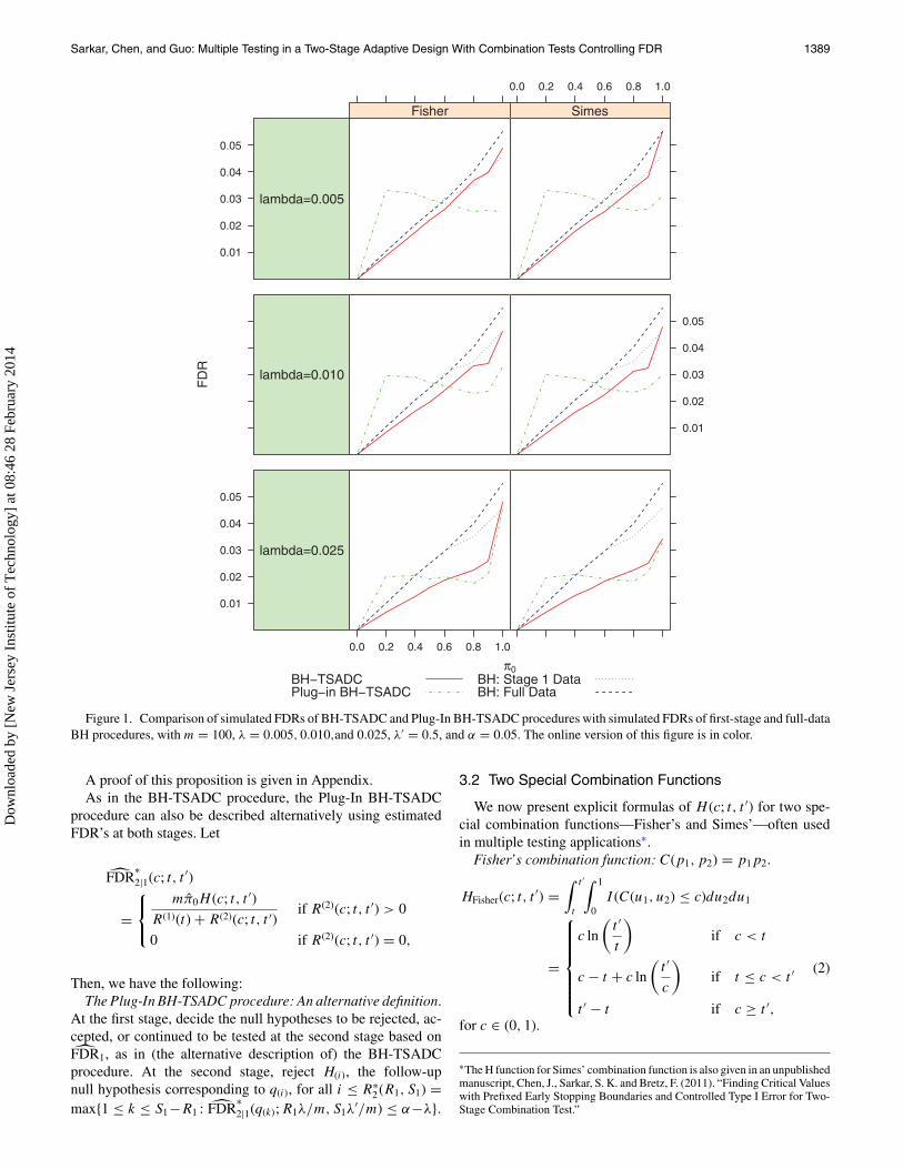
Figure 1. Comparison of simulated FDRs of BH-TSADC and Plug-In BH-TSADC procedures with simulated FDRs of first-stage and full-dataBH procedures, with m = 100, λ = 0.005, 0.010,and 0.025, λ′ = 0.5, and α = 0.05. The online version of this figure is in color.
A proof of this proposition is given in Appendix.As in the BH-TSADC procedure, the Plug-In BH-TSADC
procedure can also be described alternatively using estimatedFDR’s at both stages. Let
FDR∗2|1(c; t, t ′)
=⎧⎨⎩
mπ0H (c; t, t ′)R(1)(t) + R(2)(c; t, t ′)
if R(2)(c; t, t ′) > 0
0 if R(2)(c; t, t ′) = 0,
Then, we have the following:The Plug-In BH-TSADC procedure: An alternative definition.
At the first stage, decide the null hypotheses to be rejected, ac-cepted, or continued to be tested at the second stage based onFDR1, as in (the alternative description of) the BH-TSADCprocedure. At the second stage, reject H(i), the follow-upnull hypothesis corresponding to q(i), for all i ≤ R∗
2 (R1, S1) =max{1 ≤ k ≤ S1−R1 : FDR
∗2|1(q(k); R1λ/m, S1λ
′/m) ≤ α−λ}.
3.2 Two Special Combination Functions
We now present explicit formulas of H (c; t, t ′) for two spe-cial combination functions—Fisher’s and Simes’—often usedin multiple testing applications∗.
Fisher’s combination function: C(p1, p2) = p1p2.
HFisher(c; t, t ′) =∫ t ′
t
∫ 1
0I (C(u1, u2) ≤ c)du2du1
=
⎧⎪⎪⎪⎪⎪⎨⎪⎪⎪⎪⎪⎩c ln
(t ′
t
)if c < t
c − t + c ln
(t ′
c
)if t ≤ c < t ′
t ′ − t if c ≥ t ′,
(2)
for c ∈ (0, 1).
∗The H function for Simes’ combination function is also given in an unpublishedmanuscript, Chen, J., Sarkar, S. K. and Bretz, F. (2011). “Finding Critical Valueswith Prefixed Early Stopping Boundaries and Controlled Type I Error for Two-Stage Combination Test.”
Dow
nloa
ded
by [
New
Jer
sey
Inst
itute
of
Tec
hnol
ogy]
at 0
8:46
28
Febr
uary
201
4
1390 Journal of the American Statistical Association, December 2013
π0
pow
er
0.2
0.4
0.6
0.8
1.0Fisher
lambda=0.005
0.0 0.2 0.4 0.6 0.8 1.0
Simes
a
Fisher
lambda=0.010
0.2
0.4
0.6
0.8
1.0Simes
a
0.2
0.4
0.6
0.8
1.0
0.0 0.2 0.4 0.6 0.8 1.0
Fisher
lambda=0.025
Simes
a
BH−TSADCPlug−in BH−TSADC
BH: Stage 1 DataBH: Full Data
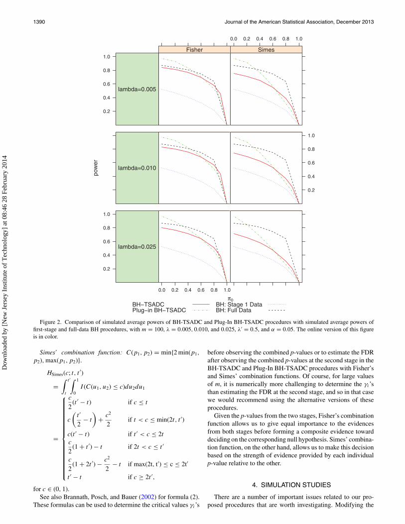
Figure 2. Comparison of simulated average powers of BH-TSADC and Plug-In BH-TSADC procedures with simulated average powers offirst-stage and full-data BH procedures, with m = 100, λ = 0.005, 0.010, and 0.025, λ′ = 0.5, and α = 0.05. The online version of this figureis in color.
Simes’ combination function: C(p1, p2) = min{2 min(p1,
p2), max(p1, p2)}.HSimes(c; t, t ′)
=∫ t ′
t
∫ 1
0I (C(u1, u2) ≤ c)du2du1
=
⎧⎪⎪⎪⎪⎪⎪⎪⎪⎪⎪⎪⎪⎪⎪⎪⎨⎪⎪⎪⎪⎪⎪⎪⎪⎪⎪⎪⎪⎪⎪⎪⎩
c
2(t ′ − t) if c ≤ t
c
(t ′
2− t
)+ c2
2if t < c ≤ min(2t, t ′)
c(t ′ − t) if t ′ < c ≤ 2t
c
2(1 + t ′) − t if 2t < c ≤ t ′
c
2(1 + 2t ′) − c2
2− t if max(2t, t′) ≤ c ≤ 2t′
t ′ − t if c ≥ 2t ′,
for c ∈ (0, 1).See also Brannath, Posch, and Bauer (2002) for formula (2).
These formulas can be used to determine the critical values γi’s
before observing the combined p-values or to estimate the FDRafter observing the combined p-values at the second stage in theBH-TSADC and Plug-In BH-TSADC procedures with Fisher’sand Simes’ combination functions. Of course, for large valuesof m, it is numerically more challenging to determine the γi’sthan estimating the FDR at the second stage, and so in that casewe would recommend using the alternative versions of theseprocedures.
Given the p-values from the two stages, Fisher’s combinationfunction allows us to give equal importance to the evidencesfrom both stages before forming a composite evidence towarddeciding on the corresponding null hypothesis. Simes’ combina-tion function, on the other hand, allows us to make this decisionbased on the strength of evidence provided by each individualp-value relative to the other.
4. SIMULATION STUDIES
There are a number of important issues related to our pro-posed procedures that are worth investigating. Modifying the
Dow
nloa
ded
by [
New
Jer
sey
Inst
itute
of
Tec
hnol
ogy]
at 0
8:46
28
Febr
uary
201
4
Sarkar, Chen, and Guo: Multiple Testing in a Two-Stage Adaptive Design With Combination Tests Controlling FDR 1391
π0
FD
R
0.01
0.02
0.03
0.04
0.05
Fisher
lambda=0.005
0.0 0.2 0.4 0.6 0.8 1.0
Simes
a
Fisher
lambda=0.010
0.01
0.02
0.03
0.04
0.05
Simes
a
0.01
0.02
0.03
0.04
0.05
0.0 0.2 0.4 0.6 0.8 1.0
Fisher
lambda=0.025
Simes
a
BH−TSADCPlug−in BH−TSADC
BH: Stage 1 DataBH: Full Data
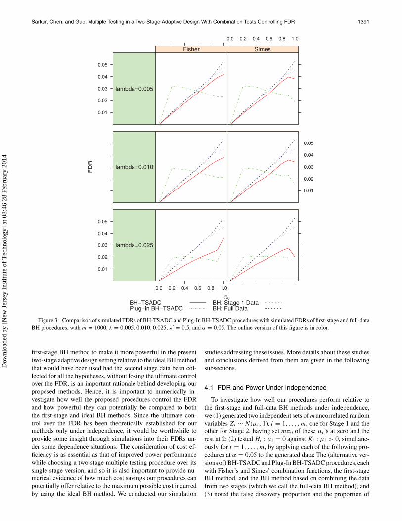
Figure 3. Comparison of simulated FDRs of BH-TSADC and Plug-In BH-TSADC procedures with simulated FDRs of first-stage and full-dataBH procedures, with m = 1000, λ = 0.005, 0.010, 0.025, λ′ = 0.5, and α = 0.05. The online version of this figure is in color.
first-stage BH method to make it more powerful in the presenttwo-stage adaptive design setting relative to the ideal BH methodthat would have been used had the second stage data been col-lected for all the hypotheses, without losing the ultimate controlover the FDR, is an important rationale behind developing ourproposed methods. Hence, it is important to numerically in-vestigate how well the proposed procedures control the FDRand how powerful they can potentially be compared to boththe first-stage and ideal BH methods. Since the ultimate con-trol over the FDR has been theoretically established for ourmethods only under independence, it would be worthwhile toprovide some insight through simulations into their FDRs un-der some dependence situations. The consideration of cost ef-ficiency is as essential as that of improved power performancewhile choosing a two-stage multiple testing procedure over itssingle-stage version, and so it is also important to provide nu-merical evidence of how much cost savings our procedures canpotentially offer relative to the maximum possible cost incurredby using the ideal BH method. We conducted our simulation
studies addressing these issues. More details about these studiesand conclusions derived from them are given in the followingsubsections.
4.1 FDR and Power Under Independence
To investigate how well our procedures perform relative tothe first-stage and full-data BH methods under independence,we (1) generated two independent sets of m uncorrelated randomvariables Zi ∼ N (μi, 1), i = 1, . . . , m, one for Stage 1 and theother for Stage 2, having set mπ0 of these μi’s at zero and therest at 2; (2) tested Hi : μi = 0 against Ki : μi > 0, simultane-ously for i = 1, . . . , m, by applying each of the following pro-cedures at α = 0.05 to the generated data: The (alternative ver-sions of) BH-TSADC and Plug-In BH-TSADC procedures, eachwith Fisher’s and Simes’ combination functions, the first-stageBH method, and the BH method based on combining the datafrom two stages (which we call the full-data BH method); and(3) noted the false discovery proportion and the proportion of
Dow
nloa
ded
by [
New
Jer
sey
Inst
itute
of
Tec
hnol
ogy]
at 0
8:46
28
Febr
uary
201
4
1392 Journal of the American Statistical Association, December 2013
π0
pow
er
0.2
0.4
0.6
0.8
1.0Fisher
lambda=0.005
0.0 0.2 0.4 0.6 0.8 1.0
Simes
a
Fisher
lambda=0.010
0.2
0.4
0.6
0.8
1.0Simes
a
0.2
0.4
0.6
0.8
1.0
0.0 0.2 0.4 0.6 0.8 1.0
Fisher
lambda=0.025
Simes
a
BH−TSADCPlug−in BH−TSADC
BH: Stage 1 DataBH: Full Data
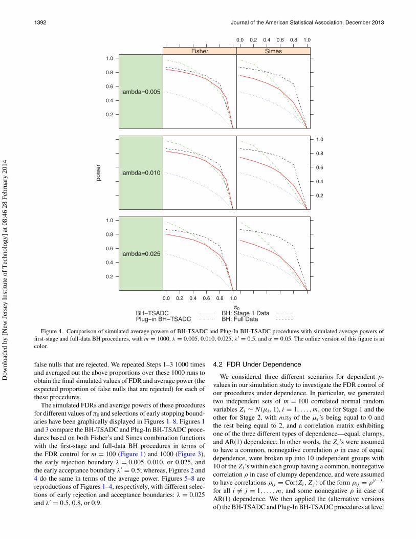
Figure 4. Comparison of simulated average powers of BH-TSADC and Plug-In BH-TSADC procedures with simulated average powers offirst-stage and full-data BH procedures, with m = 1000, λ = 0.005, 0.010, 0.025, λ′ = 0.5, and α = 0.05. The online version of this figure is incolor.
false nulls that are rejected. We repeated Steps 1–3 1000 timesand averaged out the above proportions over these 1000 runs toobtain the final simulated values of FDR and average power (theexpected proportion of false nulls that are rejected) for each ofthese procedures.
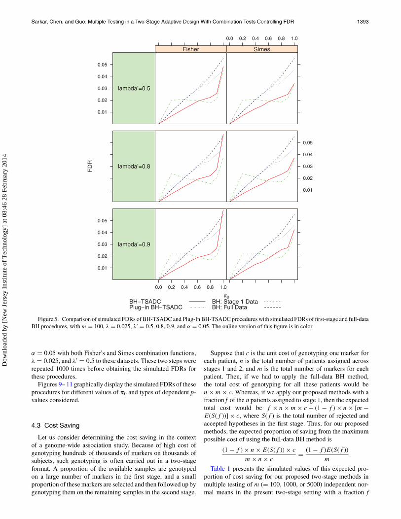
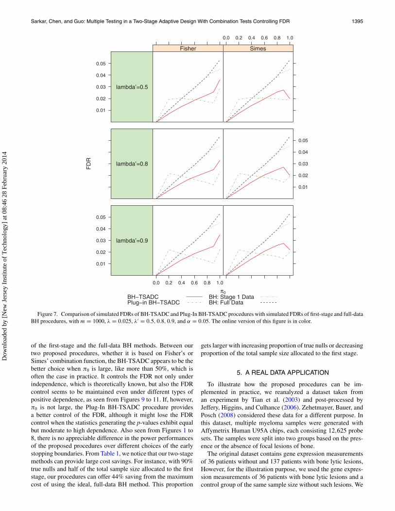
The simulated FDRs and average powers of these proceduresfor different values of π0 and selections of early stopping bound-aries have been graphically displayed in Figures 1–8. Figures 1and 3 compare the BH-TSADC and Plug-In BH-TSADC proce-dures based on both Fisher’s and Simes combination functionswith the first-stage and full-data BH procedures in terms ofthe FDR control for m = 100 (Figure 1) and 1000 (Figure 3),the early rejection boundary λ = 0.005, 0.010, or 0.025, andthe early acceptance boundary λ′ = 0.5; whereas, Figures 2 and4 do the same in terms of the average power. Figures 5–8 arereproductions of Figures 1–4, respectively, with different selec-tions of early rejection and acceptance boundaries: λ = 0.025and λ′ = 0.5, 0.8, or 0.9.
4.2 FDR Under Dependence
We considered three different scenarios for dependent p-values in our simulation study to investigate the FDR control ofour procedures under dependence. In particular, we generatedtwo independent sets of m = 100 correlated normal randomvariables Zi ∼ N (μi, 1), i = 1, . . . , m, one for Stage 1 and theother for Stage 2, with mπ0 of the μi’s being equal to 0 andthe rest being equal to 2, and a correlation matrix exhibitingone of the three different types of dependence—equal, clumpy,and AR(1) dependence. In other words, the Zi’s were assumedto have a common, nonnegative correlation ρ in case of equaldependence, were broken up into 10 independent groups with10 of the Zi’s within each group having a common, nonnegativecorrelation ρ in case of clumpy dependence, and were assumedto have correlations ρij = Cor(Zi, Zj ) of the form ρij = ρ|i−j |
for all i = j = 1, . . . , m, and some nonnegative ρ in case ofAR(1) dependence. We then applied the (alternative versionsof) the BH-TSADC and Plug-In BH-TSADC procedures at level
Dow
nloa
ded
by [
New
Jer
sey
Inst
itute
of
Tec
hnol
ogy]
at 0
8:46
28
Febr
uary
201
4
Sarkar, Chen, and Guo: Multiple Testing in a Two-Stage Adaptive Design With Combination Tests Controlling FDR 1393
π0
FD
R
0.01
0.02
0.03
0.04
0.05
Fisher
lambda’=0.5
0.0 0.2 0.4 0.6 0.8 1.0
Simes
Fisher
lambda’=0.8
0.01
0.02
0.03
0.04
0.05
Simes
0.01
0.02
0.03
0.04
0.05
0.0 0.2 0.4 0.6 0.8 1.0
Fisher
lambda’=0.9
Simes
BH−TSADCPlug−in BH−TSADC
BH: Stage 1 DataBH: Full Data
Figure 5. Comparison of simulated FDRs of BH-TSADC and Plug-In BH-TSADC procedures with simulated FDRs of first-stage and full-dataBH procedures, with m = 100, λ = 0.025, λ′ = 0.5, 0.8, 0.9, and α = 0.05. The online version of this figure is in color.
α = 0.05 with both Fisher’s and Simes combination functions,λ = 0.025, and λ′ = 0.5 to these datasets. These two steps wererepeated 1000 times before obtaining the simulated FDRs forthese procedures.
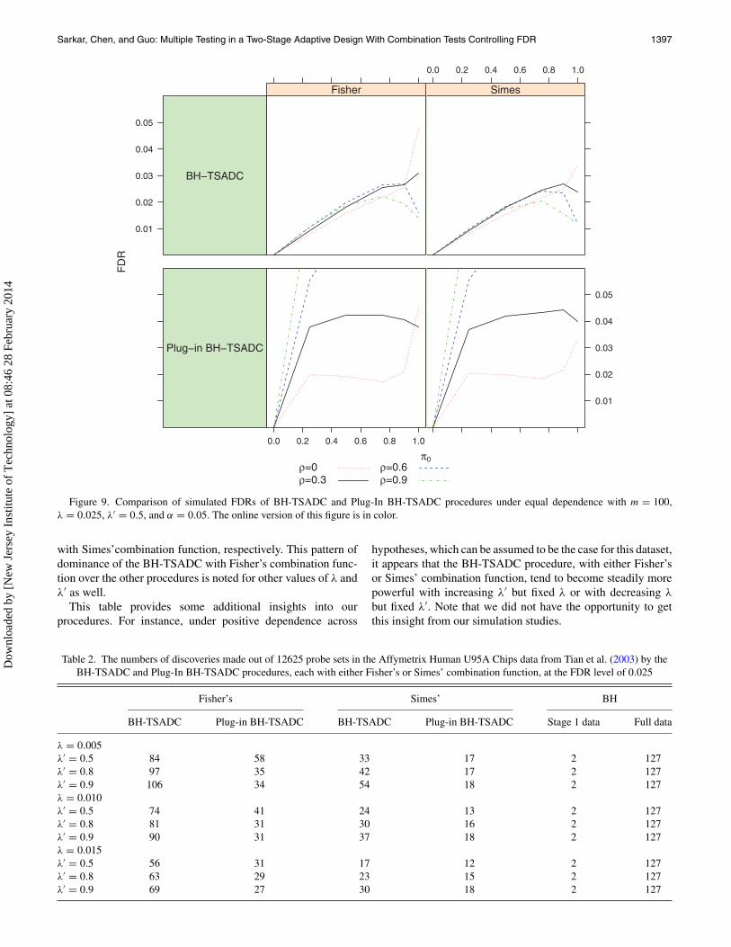
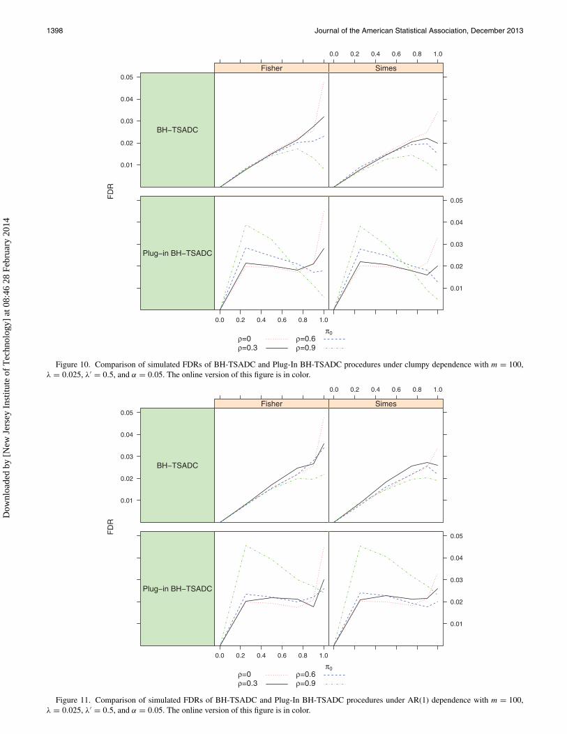
Figures 9– 11 graphically display the simulated FDRs of theseprocedures for different values of π0 and types of dependent p-values considered.
4.3 Cost Saving
Let us consider determining the cost saving in the contextof a genome-wide association study. Because of high cost ofgenotyping hundreds of thousands of markers on thousands ofsubjects, such genotyping is often carried out in a two-stageformat. A proportion of the available samples are genotypedon a large number of markers in the first stage, and a smallproportion of these markers are selected and then followed up bygenotyping them on the remaining samples in the second stage.
Suppose that c is the unit cost of genotyping one marker foreach patient, n is the total number of patients assigned acrossstages 1 and 2, and m is the total number of markers for eachpatient. Then, if we had to apply the full-data BH method,the total cost of genotyping for all these patients would ben × m × c. Whereas, if we apply our proposed methods with afraction f of the n patients assigned to stage 1, then the expectedtotal cost would be f × n × m × c + (1 − f ) × n × [m −E(S(f ))] × c, where S(f ) is the total number of rejected andaccepted hypotheses in the first stage. Thus, for our proposedmethods, the expected proportion of saving from the maximumpossible cost of using the full-data BH method is
(1 − f ) × n × E(S(f )) × c
m × n × c= (1 − f )E(S(f ))
m.
Table 1 presents the simulated values of this expected pro-portion of cost saving for our proposed two-stage methods inmultiple testing of m (= 100, 1000, or 5000) independent nor-mal means in the present two-stage setting with a fraction f
Dow
nloa
ded
by [
New
Jer
sey
Inst
itute
of
Tec
hnol
ogy]
at 0
8:46
28
Febr
uary
201
4
1394 Journal of the American Statistical Association, December 2013
π0
pow
er
0.2
0.4
0.6
0.8
1.0Fisher
lambda’=0.5
0.0 0.2 0.4 0.6 0.8 1.0
Simes
Fisher
lambda’=0.8
0.2
0.4
0.6
0.8
1.0Simes
0.2
0.4
0.6
0.8
1.0
0.0 0.2 0.4 0.6 0.8 1.0
Fisher
lambda’=0.9
Simes
BH−TSADCPlug−in BH−TSADC
BH: Stage 1 DataBH: Full Data
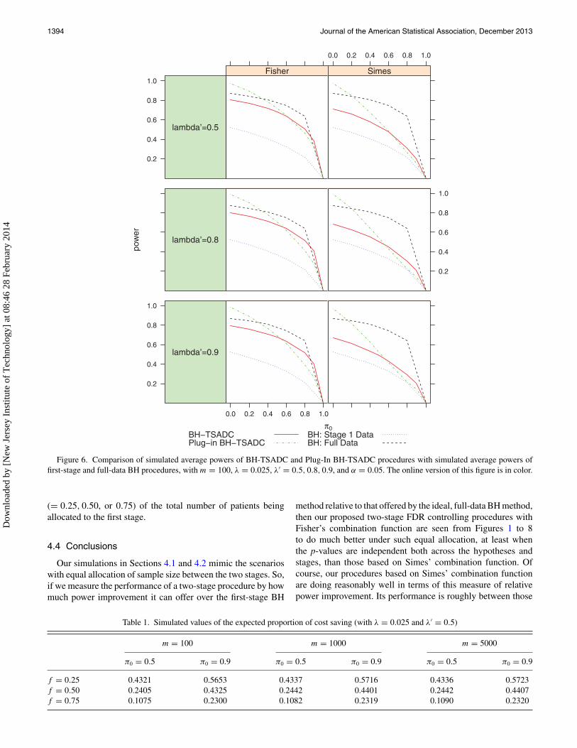
Figure 6. Comparison of simulated average powers of BH-TSADC and Plug-In BH-TSADC procedures with simulated average powers offirst-stage and full-data BH procedures, with m = 100, λ = 0.025, λ′ = 0.5, 0.8, 0.9, and α = 0.05. The online version of this figure is in color.
(= 0.25, 0.50, or 0.75) of the total number of patients beingallocated to the first stage.
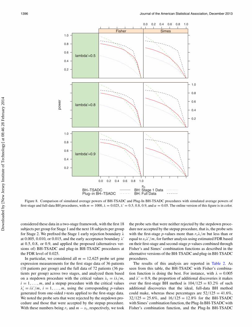
4.4 Conclusions
Our simulations in Sections 4.1 and 4.2 mimic the scenarioswith equal allocation of sample size between the two stages. So,if we measure the performance of a two-stage procedure by howmuch power improvement it can offer over the first-stage BH
method relative to that offered by the ideal, full-data BH method,then our proposed two-stage FDR controlling procedures withFisher’s combination function are seen from Figures 1 to 8to do much better under such equal allocation, at least whenthe p-values are independent both across the hypotheses andstages, than those based on Simes’ combination function. Ofcourse, our procedures based on Simes’ combination functionare doing reasonably well in terms of this measure of relativepower improvement. Its performance is roughly between those
Table 1. Simulated values of the expected proportion of cost saving (with λ = 0.025 and λ′ = 0.5)
m = 100 m = 1000 m = 5000
π0 = 0.5 π0 = 0.9 π0 = 0.5 π0 = 0.9 π0 = 0.5 π0 = 0.9
f = 0.25 0.4321 0.5653 0.4337 0.5716 0.4336 0.5723f = 0.50 0.2405 0.4325 0.2442 0.4401 0.2442 0.4407f = 0.75 0.1075 0.2300 0.1082 0.2319 0.1090 0.2320
Dow
nloa
ded
by [
New
Jer
sey
Inst
itute
of
Tec
hnol
ogy]
at 0
8:46
28
Febr
uary
201
4
Sarkar, Chen, and Guo: Multiple Testing in a Two-Stage Adaptive Design With Combination Tests Controlling FDR 1395
π0
FD
R
0.01
0.02
0.03
0.04
0.05
Fisher
lambda’=0.5
0.0 0.2 0.4 0.6 0.8 1.0
Simes
Fisher
lambda’=0.8
0.01
0.02
0.03
0.04
0.05
Simes
0.01
0.02
0.03
0.04
0.05
0.0 0.2 0.4 0.6 0.8 1.0
Fisher
lambda’=0.9
Simes
BH−TSADCPlug−in BH−TSADC
BH: Stage 1 DataBH: Full Data
Figure 7. Comparison of simulated FDRs of BH-TSADC and Plug-In BH-TSADC procedures with simulated FDRs of first-stage and full-dataBH procedures, with m = 1000, λ = 0.025, λ′ = 0.5, 0.8, 0.9, and α = 0.05. The online version of this figure is in color.
of the first-stage and the full-data BH methods. Between ourtwo proposed procedures, whether it is based on Fisher’s orSimes’ combination function, the BH-TSADC appears to be thebetter choice when π0 is large, like more than 50%, which isoften the case in practice. It controls the FDR not only underindependence, which is theoretically known, but also the FDRcontrol seems to be maintained even under different types ofpositive dependence, as seen from Figures 9 to 11. If, however,π0 is not large, the Plug-In BH-TSADC procedure providesa better control of the FDR, although it might lose the FDRcontrol when the statistics generating the p-values exhibit equalbut moderate to high dependence. Also seen from Figures 1 to8, there is no appreciable difference in the power performancesof the proposed procedures over different choices of the earlystopping boundaries. From Table 1, we notice that our two-stagemethods can provide large cost savings. For instance, with 90%true nulls and half of the total sample size allocated to the firststage, our procedures can offer 44% saving from the maximumcost of using the ideal, full-data BH method. This proportion
gets larger with increasing proportion of true nulls or decreasingproportion of the total sample size allocated to the first stage.
5. A REAL DATA APPLICATION
To illustrate how the proposed procedures can be im-plemented in practice, we reanalyzed a dataset taken froman experiment by Tian et al. (2003) and post-processed byJeffery, Higgins, and Culhance (2006). Zehetmayer, Bauer, andPosch (2008) considered these data for a different purpose. Inthis dataset, multiple myeloma samples were generated withAffymetrix Human U95A chips, each consisting 12,625 probesets. The samples were split into two groups based on the pres-ence or the absence of focal lesions of bone.
The original dataset contains gene expression measurementsof 36 patients without and 137 patients with bone lytic lesions,However, for the illustration purpose, we used the gene expres-sion measurements of 36 patients with bone lytic lesions and acontrol group of the same sample size without such lesions. We
Dow
nloa
ded
by [
New
Jer
sey
Inst
itute
of
Tec
hnol
ogy]
at 0
8:46
28
Febr
uary
201
4
1396 Journal of the American Statistical Association, December 2013
π0
pow
er
0.2
0.4
0.6
0.8
1.0Fisher
lambda’=0.5
0.0 0.2 0.4 0.6 0.8 1.0
Simes
Fisher
lambda’=0.8
0.2
0.4
0.6
0.8
1.0Simes
0.2
0.4
0.6
0.8
1.0
0.0 0.2 0.4 0.6 0.8 1.0
Fisher
lambda’=0.9
Simes
BH−TSADCPlug−in BH−TSADC
BH: Stage 1 DataBH: Full Data
Figure 8. Comparison of simulated average powers of BH-TSADC and Plug-In BH-TSADC procedures with simulated average powers offirst-stage and full-data BH procedures, with m = 1000, λ = 0.025, λ′ = 0.5, 0.8, 0.9, and α = 0.05. The online version of this figure is in color.
considered these data in a two-stage framework, with the first 18subjects per group for Stage 1 and the next 18 subjects per groupfor Stage 2. We prefixed the Stage 1 early rejection boundary λ
at 0.005, 0.010, or 0.015, and the early acceptance boundary λ′
at 0.5, 0.8, or 0.9, and applied the proposed (alternatives ver-sions of) BH-TSADC and plug-in BH-TSADC procedures atthe FDR level of 0.025.
In particular, we considered all m = 12,625 probe set geneexpression measurements for the first stage data of 36 patients(18 patients per group) and the full data of 72 patients (36 pa-tients per group) across two stages, and analyzed them basedon a stepdown procedure with the critical values λi = iλ/m,i = 1, . . . , m, and a stepup procedure with the critical valuesλ′
i = iλ′/m, i = 1, . . . , m, using the corresponding p-valuesgenerated from one-sided t-tests applied to the first-stage data.We noted the probe sets that were rejected by the stepdown pro-cedure and those that were accepted by the stepup procedure.With these numbers being r1 and m − s1, respectively, we took
the probe sets that were neither rejected by the stepdown proce-dure nor accepted by the stepup procedure, that is, the probe setswith the first-stage p-values more than r1λ/m but less than orequal to s1λ
′/m, for further analysis using estimated FDR basedon their first-stage and second-stage p-values combined throughFisher’s and Simes’ combination functions as described in thealternative versions of the BH-TSADC and plug-in BH-TSADCprocedures.
The results of this analysis are reported in Table 2. Asseen from this table, the BH-TSADC with Fisher’s combina-tion function is doing the best. For instance, with λ = 0.005and λ′ = 0.9, the proportion of additional discoveries it makesover the first-stage BH method is 104/125 = 83.2% of suchadditional discoveries that the ideal, full-data BH methodcould make, whereas these percentages are 52/125 = 41.6%,32/125 = 25.6%, and 16/125 = 12.8% for the BH-TSADCwith Simes’ combination function, the Plug-In BH-TSADC withFisher’s combination function, and the Plug-In BH-TSADC
Dow
nloa
ded
by [
New
Jer
sey
Inst
itute
of
Tec
hnol
ogy]
at 0
8:46
28
Febr
uary
201
4
Sarkar, Chen, and Guo: Multiple Testing in a Two-Stage Adaptive Design With Combination Tests Controlling FDR 1397
π0
FD
R
0.01
0.02
0.03
0.04
0.05
Fisher
BH−TSADC
0.0 0.2 0.4 0.6 0.8 1.0
Simes
S
0.0 0.2 0.4 0.6 0.8 1.0
Fisher
Plug−in BH−TSADC
0.01
0.02
0.03
0.04
0.05
Simes
H
ρ=0ρ=0.3
ρ=0.6ρ=0.9
Figure 9. Comparison of simulated FDRs of BH-TSADC and Plug-In BH-TSADC procedures under equal dependence with m = 100,λ = 0.025, λ′ = 0.5, and α = 0.05. The online version of this figure is in color.
with Simes’combination function, respectively. This pattern ofdominance of the BH-TSADC with Fisher’s combination func-tion over the other procedures is noted for other values of λ andλ′ as well.
This table provides some additional insights into ourprocedures. For instance, under positive dependence across
hypotheses, which can be assumed to be the case for this dataset,it appears that the BH-TSADC procedure, with either Fisher’sor Simes’ combination function, tend to become steadily morepowerful with increasing λ′ but fixed λ or with decreasing λ
but fixed λ′. Note that we did not have the opportunity to getthis insight from our simulation studies.
Table 2. The numbers of discoveries made out of 12625 probe sets in the Affymetrix Human U95A Chips data from Tian et al. (2003) by theBH-TSADC and Plug-In BH-TSADC procedures, each with either Fisher’s or Simes’ combination function, at the FDR level of 0.025
Fisher’s Simes’ BH
BH-TSADC Plug-in BH-TSADC BH-TSADC Plug-in BH-TSADC Stage 1 data Full data
λ = 0.005λ′ = 0.5 84 58 33 17 2 127λ′ = 0.8 97 35 42 17 2 127λ′ = 0.9 106 34 54 18 2 127λ = 0.010λ′ = 0.5 74 41 24 13 2 127λ′ = 0.8 81 31 30 16 2 127λ′ = 0.9 90 31 37 18 2 127λ = 0.015λ′ = 0.5 56 31 17 12 2 127λ′ = 0.8 63 29 23 15 2 127λ′ = 0.9 69 27 30 18 2 127
Dow
nloa
ded
by [
New
Jer
sey
Inst
itute
of
Tec
hnol
ogy]
at 0
8:46
28
Febr
uary
201
4
1398 Journal of the American Statistical Association, December 2013
π0
FD
R
0.01
0.02
0.03
0.04
0.05Fisher
BH−TSADC
0.0 0.2 0.4 0.6 0.8 1.0
Simes
S
0.0 0.2 0.4 0.6 0.8 1.0
Fisher
Plug−in BH−TSADC
0.01
0.02
0.03
0.04
0.05Simes
H
ρ=0ρ=0.3
ρ=0.6ρ=0.9
Figure 10. Comparison of simulated FDRs of BH-TSADC and Plug-In BH-TSADC procedures under clumpy dependence with m = 100,λ = 0.025, λ′ = 0.5, and α = 0.05. The online version of this figure is in color.
π0
FD
R
0.01
0.02
0.03
0.04
0.05Fisher
BH−TSADC
0.0 0.2 0.4 0.6 0.8 1.0
Simes
S
0.0 0.2 0.4 0.6 0.8 1.0
Fisher
Plug−in BH−TSADC
0.01
0.02
0.03
0.04
0.05Simes
H
ρ=0ρ=0.3
ρ=0.6ρ=0.9
Figure 11. Comparison of simulated FDRs of BH-TSADC and Plug-In BH-TSADC procedures under AR(1) dependence with m = 100,λ = 0.025, λ′ = 0.5, and α = 0.05. The online version of this figure is in color.
Dow
nloa
ded
by [
New
Jer
sey
Inst
itute
of
Tec
hnol
ogy]
at 0
8:46
28
Febr
uary
201
4
Sarkar, Chen, and Guo: Multiple Testing in a Two-Stage Adaptive Design With Combination Tests Controlling FDR 1399
6. CONCLUDING REMARKS
This article has been motivated by the need to have a two-stage strategy for testing multiple null hypotheses, not knownbefore, that allows making early decisions on the null hypothe-ses in terms of rejection, acceptance, or continuation to thesecond stage for further testing with more observations, andeventually controls the FDR in a nonasymptotic setting, as thefirst step toward designing an FDR based two-stage study. Wehave produced two such strategies by generalizing the classicalBH method and its adaptive version from single-stage to thepresent two-stage setting. We have proved their FDR controlunder independence and provided simulation evidence showingtheir meaningful improvements over the first-stage BH methodrelative to those ideally offered by the full-data BH method interms of both power and cost savings, and given an example oftheir utilities in practice. We also have presented numerical ev-idence that the proposed strategies can maintain a control overthe FDR even under some dependence situations.
Now that we know how to test multiple hypotheses in thepresent two-stage adaptive design format controlling the FDR,we can get to addressing issues related to designing FDR basedtwo-stage studies. One such issue is optimal allocation of samplesizes to the two stages. Let us briefly outline the steps one cantake toward addressing this issue.
Suppose that we have a study involving m genes, andour problem is to identify the differentially expressed genesbetween two independent groups by simultaneously testingHi : δi = 0 against Ki : δi = 0 for i = 1, . . . , m, where δi =(μix − μiy)/σi is the (standardized) effect size defined in termsof μix and μiy , the group means, and σ 2
i , the common group vari-ance, for the ith gene, given that we decide to have the maximumN number of observations per gene for all the groups and stagescombined and choose some fixed early stopping boundariesλ < λ′. Assume that the observed expression levels for eachgroup follow normal distributions, with proper normalization,so that we can apply the two-sample t test once such observationsare available. We consider using equal sample size per groupfor this test. An optimal FDR based two-stage design based onour method of multiple testing can be constructed as follows.
Assume that we take n1 = Nf/2 observations per group foreach gene at the first stage, for some fraction 0 < f < 1, and ad-ditional n2 = N (1 − f )/2 observations per group for each of them − S(f ) follow-up genes, where S(f ) denotes (as in Section3.4) the total number of rejected and accepted null hypothesesat the first stage. Let xi1 and yi1 be the estimates of μix and μiy ,respectively, and s2
i1 be the pooled estimate of σ 2i , for the ith
gene based on the first-stage observations, and xi2, yi2, and s2i2
be those estimates based on the additional observations for theith follow-up gene. Let tij = (xij − yij )/sij
√2/nj = δi
√nj/2,
where δij = (Xij − Yij )/sij , for i = 1, . . . , m, j = 1, 2. Then,pi1 = 2[1 − G1(|ti1|) is the first-stage p-value for the ith gene,for i = 1, . . . , m, and pi2 = 2[1 − G2(|ti2|) is the second-stagep-value for the ith follow-up gene, where Gj is the cumulativedistribution function of the central t distribution with nj − 2degrees of freedom.
Now, if we find the f for which our proposed two-stagemethod of multiple testing based on these first- and second-stagep-values maximize the average power at specified alternatives
for some targeted genes, then that f will provide a good FDRbased two-stage design, given N, λ and λ′. Of course, it bringsforth some newer and interesting theoretical issues that need tobe addressed.
We have proposed our FDR controlling procedures in thisarticle considering a nonasymptotic setting. However, one mayconsider developing procedures that would asymptotically con-trol the FDR by taking the following approach toward findingthe first- and second-stage thresholds subject to the early bound-aries λ < λ′ and the final boundary α on the FDR. Given twoconstants t < t ′, consider making an early decision regardingHi by rejecting it if p1i ≤ t , accepting it if p1i > t ′, and contin-uing to test it at the second stage if t < p1i ≤ t ′. At the secondstage, reject Hi if C(p1i , p2i) ≤ c. Storey’s (2002) estimate ofthe FDR at the first-stage is given by
FDR∗1(t) =
⎧⎨⎩mπ0t
R(1)(t)if R(1)(t) > 0
0 if R(1)(t) = 0,
for some estimate π0 of π0. Similarly, the cumulative FDR atthe second stage can be estimated as follows:
FDR∗2(c, t, t ′)
=⎧⎨⎩
mπ0[t + H (c; t, t ′)]R(1)(t) + R(2)(c; t, t ′)
if R(1)(t) + R(2)(c; t, t ′) > 0
0 if R(1)(t) + R(2)(c; t, t ′) = 0
Let
tλ = sup{t : FDR1(t ′) ≤ λ for all t ′ ≤ t},tλ′ = inf{t : FDR1(t ′) > λ′ for all t ′ > t},
and
cα(λ, λ′) = sup{c : FDR2(c, tλ, tλ′ ) ≤ α}.Then, reject Hi if p1i ≤ tλ or if tλ < p1i ≤ tλ′ and C(p1i , p2i) ≤cα(λ, λ′). This may control the overall FDR asymptotically un-der the weak dependence condition and the consistency propertyof π0 (as in Storey, Taylor, and Siegmund 2004).
The foregoing discussion also suggests how to estimate theFDR for each hypothesis in a completed two-stage design ofthe present form. For instance, for hypothesis with the pair ofp-values (p1, p2), the estimated FDR is FDR
∗1(p1) if p1 ≤ tλ or
p1 ≥ tλ′ , and is FDR∗2(c(p1, p2), tλ, tλ′) if tλ < p1 < tλ′ .
There is another important issue related to the present prob-lem which we have not touched in this article but hope to ad-dress in a different communication. There are other combinationfunctions, such as Fisher’s weighted product (Fisher 1932) andweighted inverse normal (Mosteller and Bush 1954); their per-formances would be worth investigating.
APPENDIX
Proof of Theorem 1.
FDR12 = E
[V1 + V2
max{R1 + R2, 1}]
≤ E
[V1
max{R1, 1}]
+ E
[V2
max{R1 + R2, 1}].
Dow
nloa
ded
by [
New
Jer
sey
Inst
itute
of
Tec
hnol
ogy]
at 0
8:46
28
Febr
uary
201
4
1400 Journal of the American Statistical Association, December 2013
Now,
E
[V1
max{R1, 1}]
=∑i∈J0
E
[I (p1i ≤ λR1 )
max{R1, 1}]
≤∑i∈J0
E
[I(p1i ≤ λ
R(−i)1 +1
)R
(−i)1 + 1
];
(as shown in Sarkar 2008; see also Result 1). And,
E
[V2
max{R1 + R2, 1}]
=∑i∈J0
E
×[
I (λR1+1 < p1i ≤ λ′S1
, qi ≤ γR1+R2,S1 , S1 > R1, R2 > 0)
R1 + R2
].
(A.1)
Writing R2 more explicitly in terms of R1 and S1, we see that theexpression in Equation (3) is equal to
∑i∈J0
m∑s1=1
s1−1∑r1=0
s1−r1∑r2=1
E[(
I(λr1+1 < p1i ≤ λ′
s1, qi ≤ γr1+r2,s1 , R1 = r1,
S1 = s1, R2(r1, s1) = r2
))/(r1 + r2)
]=∑i∈J0
m∑s1=1
s1−1∑r1=0
s1−r1∑r2=1
E[(
I(λr1+1 < p1i ≤ λ′
s1,
qi ≤ γr1+r2,s1 R(−i)1 = r1, S
(−i)1 = s1 − 1,
R(−i)2 (r1, s1) = r2 − 1
))/(r1 + r2)
]=∑i∈J0
m−1∑s1=0
s1∑r1=0
s1−r1∑r2=0
E[(
I(λr1+1 < p1i ≤ λ′
s1+1,
qi ≤ γr1+r2+1,s1+1, R(−i)1 = r1, S
(−i)1 = s1,
R(−i)2 (r1, s1 + 1) = r2
))/(r1 + r2 + 1)
]=∑i∈J0
E[(
I(λ
R(−i)1 +1 < p1i ≤ λ′
S(−i)1 +1
,
qi ≤ γR
(−i)1 +R
(−i)2 +1,S
(−i)1 +1
))/(R
(−i)1 + R
(−i)2 + 1
)].
Thus, the theorem is proved. �
Proof of proposition 1.
FDR12 ≤∑i∈J0
E
[PrH
(p1 ≤ λ
R(−i)1 +1
)R
(−i)1 + 1
]+∑i∈J0
E
×⎡⎣PrH
(λ
R(−i)1 +1<p1 ≤λ′
S(−i)1 +1
, C(p1, p2)≤γR
(−i)1 +R
(−i)2 +1,S
(−i)1 +1
)R
(−i)1 + R
(−i)2 + 1
⎤⎦≤∑i∈J0
E
[λ
R(−i)1 +1
R(−i)1 + 1
]+∑i∈J0
E
×⎡⎣Pr
(λ
R(−i)1 +1<u1 ≤ λ′
S(−i)1 +1
, C(u1, u2) ≤ γR
(−i)1 +R
(−i)2 +1,S
(−i)1 +1
)R
(−i)1 + R
(−i)2 + 1
⎤⎦.(A.2)
The first sum in Equation (4) is less than or equal to π0λ, sinceλ
R(−i)1 +1 = [R(−i)
1 + 1]λ/m, and the second sum is less than or equal toπ0(α − λ), since the probability in the numerator in this sum is equalto
H(γ
R1(−i)+R
(−i)2 +1,S
(−i)1 +1; λ
R1(−i)+1, λ
′S
(−i)1 +1
)=[R
(−i)1 + 1 + R
(−i)2
](α − λ)
m.
Thus, the proposition is proved. �
Proof of Proposition 2. This can be proved as in Proposition 1.More specifically, first note that the FDR here, which we call theFDR∗
12, satisfies the following:
FDR∗12 ≤
∑i∈J0
E
[I(p1i ≤ λ
R(−i)1 +1
)R
(−i)1 + 1
]+∑i∈J0
E
×⎡⎣I(λ
R(−i)1 +1 ≤ p1i ≤ λ′
S(−i)1 +1
, qi≤γ ∗R
(−i)1 +R
∗(−i)2 +1,S
(−i)1 +1
)R
(−i)1 + R
∗(−i)2 + 1
⎤⎦,(A.3)
where
R∗(−i)2 ≡ R
∗(−i)2
(R
(−i)1 , S
(−i)1 + 1
)= max
{1 ≤ j ≤ S
(−i)1 − R
(−i)1 : q
(−i)(j ) ≤ γ ∗
R(−i)1 +j+1,S
(−i)1 +1
},
with q(−i)(j ) being the ordered versions of the combined p-values except
the qi . As in Proposition 1, the first sum in Equation (5) is less than orequal to π0λ. Before working with the second sum, first note that theγ ∗ satisfying Equation (1), that is, the following equation:
H(γ ∗
r1+i,s1; λr1 , λ
′s1
) = (r1 + i)(α − λ)(1 − λ′)m − s1 + 1
,
is less than or equal to the γ ∗∗ satisfying
H(γ ∗∗
r1+i,s1; λr1 , λ
′s1
) = (r1 + i)(α − λ)(1 − λ′)
m − s(−j )1
,
for any fixed j = 1, . . . , m. So, the second sum in Equation (5) is lessthan or equal to
∑i∈J0
E
⎡⎢⎣ I(λ
R(−i)1 +1 ≤ p1i ≤ λ′
S(−i)1 +1
, qi ≤ γ ∗∗R
(−i)1 +R
∗(−i)2 +1,S
(−i)1 +1
)R
(−i)1 + R
∗(−i)2 + 1
⎤⎥⎦=∑i∈J0
E
⎡⎢⎣H(γ ∗∗
R(−i)1 +R
∗(−i)2 +1,S
(−i)1 +1
; λR
(−i)1 +1, λ
′S
(−i)1 +1
)R
(−i)1 + R
∗(−i)2 + 1
⎤⎥⎦= (α − λ)
∑i∈J0
E
[1 − λ′
m − S(−i)1
]≤ α − λ,
since∑
i∈J0E[ 1−λ′
m−S(−i)1
] ≤ 1; see, for instance, Sarkar (2008, p. 151).
Hence, FDR∗12 ≤ π0λ + α − λ ≤ α, which proves the proposition. �
SUPPLEMENTARY MATERIALS
As suggested by one of the reviewers, we have examinedthe performance of our proposed procedures in a complicatedgenetic mode with exponentially decreasing effect sizes. Thesimulation results can be found in the supplementary materials.
[Received June 2011. Revised September 2012.]
REFERENCES
Benjamini, Y., and Hochberg, Y. (1995), “Controlling the False Discovery Rate:A Practical and Powerful Approach to Multiple Testing,” Journal of theRoyal Statistical Society, Series B, 57, 289–300. [1385,1386]
——— (2000), “On the Adaptive Control of the False Discovery Rate in Mul-tiple Testing With Independent Statistics,” Journal of Educational and Be-havioral Statistics, 25, 60–83. [1386]
Dow
nloa
ded
by [
New
Jer
sey
Inst
itute
of
Tec
hnol
ogy]
at 0
8:46
28
Febr
uary
201
4
Sarkar, Chen, and Guo: Multiple Testing in a Two-Stage Adaptive Design With Combination Tests Controlling FDR 1401
Benjamini, Y., Krieger, A., and Yekutieli, D. (2006), “Adaptive Linear Step-UpFalse Discovery Rate Controlling Procedures,” Biometrika, 93, 491–507.[1386]
Benjamini, Y., and Yekutieli, D. (2001), “The Control of the False DiscoveryRate in Multiple Testing Under Dependency,” The Annals of Statistics, 29,1165–1188. [1386]
Blanchard, G., and Roquain, E. (2009), “Adaptive FDR Control Under Inde-pendence and Dependence,” Journal of Machine Learning Research, 10,2837–2871. [1386]
Brannath, W., Posch, M., and Bauer, P. (2002), “Recursive CombinationTests,” Journal of the American Statistical Association, 97, 236–244.[1385,1388,1390]
Fisher, R. A. (1932), Statistical Methods for Research Workers (4th ed.),London: Oliver and Boyd. [1399]
Gavrilov, Y., Benjamini, Y., and Sarkar, S. K. (2009), “An Adaptive Step-DownProcedure With Proven FDR Control Under Independence,” The Annals ofStatistics, 37, 619–629. [1386]
Jeffery, I., Higgins, D., and Culhance, A. (2006), “Comparison and Evalua-tion of Methods for Generating Differentiall Expressed Genes Lists FromMicroarray Data,” BMC Bioinformatics, 7, 359–375. [1395]
Mosteller, F., and Bush, R. (1954), “Selected Quantitative Techniques,” inHandbook of Social Psychology, Vol. 1, ed. G. Lindzey, Cambridge, MA:Addison-Wesley, pp. 289–334. [1399]
Posch, M., Zehetmayer, S., and Bauer, P. (2009), “Hunting for Significance Withthe False Discovery Rate,” Journal of the American Statistical Association,104, 832–840. [1385]
Sarkar, S. K. (2002), “Some Results on False Discovery Rate in StepwiseMultiple Testing Procedures,” The Annals of Statistics, 30, 239–257. [1386]
——— (2008), “On Methods Controlling the False Discovery Rate,” Sankhya,Series A, 70, 135–168. [1386,1388,1400]
Storey, J. (2002), “A Direct Approach to False Discovery Rates,” Journal of theRoyal Statistical Society, Series B, 64, 479–498. [1386,1399]
Storey, J., Taylor, J., and Siegmund, D. (2004), “Strong Control, ConservativePoint Estimation and Simultaneous Conservative Consistency of False Dis-covery Rates: A Unified Approach,” Journal of the Royal Statistical Society,Series B, 66, 187–205. [1386,1388,1399]
Storey, J., and Tibshirani, R. (2003), “Statistical Significance in GenomewideStudies,” Proceedings of the National Academy of Science USA, 100,9440–9445. [1385]
Tian, E., Zhan, F., Walker, R., Rasmussen, E., Ma, Y., and Barlogie, B. (2003),“The Role of the WNT-Signaling Antagonist DKKI in the Development ofOsteolytic Lesions in Multple Myeloma,” New England Journal of Medicine,349, 2438–2494. [1395,1397]
Victor, A., and Hommel, G. (2007), “Combining Adaptive Design With Controlof the False Discovery Rate—A Generalized Definition for a Global P-value,” Biometrical Journal, 49, 94–106. [1385]
Weller, J., Song, J., Heyen, D., Lewin, H., and Ron, M. (1998), “A New Ap-proach to the Problem of Multiple Comparisons in the Genetic Dissectionof Complex Traits,” Genetics, 150, 1699–1706. [1385]
Zehetmayer, S., Bauer, P., and Posch, M. (2005), “Two-Stage Designs forExperiments With a Large Number of Hypotheses,” Bioinformatics, 21,3771–3777. [1385]
——— (2008), “Optimized Multi-Stage Designs Controlling the False Discov-ery or the Family-Wise Error Rate,” Statistics in Medicine, 27, 4145–4160.[1385,1386,1395]
Dow
nloa
ded
by [
New
Jer
sey
Inst
itute
of
Tec
hnol
ogy]
at 0
8:46
28
Febr
uary
201
4