arX

iv:h

ep-t

h/98

1006

7v1

9 O

ct 1

998

October 1998 IFT-P/067/98

hep-th/9810067

Integrable theories in any dimension

and homogenous spaces

Luiz A. Ferreira and Erica E. Leite

Instituto de Fısica Teorica - IFT/UNESP

Rua Pamplona 145

01405-900 Sao Paulo-SP, BRAZIL

Abstract

We construct local zero curvature representations for non-linear sigma models

on homogeneous spaces, defined on a space-time of any dimension, following a

recently proposed approach to integrable theories in dimensions higher than two.

We present some sufficient conditions for the existence of integrable submodels

possessing an infinite number of local conservation laws. Examples involving

symmetric spaces and group manifolds are given. The CPN models are discussed

in detail.

1 Introduction

The development of techniques to study non-perturbative aspects of physical theories

is of crucial importance in practically all areas of Physics. Many open problems in high

energy physics can not be studied with conventional perturbative methods, and they

are in fact related to the non-linear character of the Lorentz invariant field theories

describing the fundamental interactions of Nature.

It is perhaps correct to say that many of the developments obtained so far in

such area involve, in one way or the other, soliton solutions. The most recent and

striking examples are the exact results obtained about the strong coupling regime of

supersymmetric gauge theories [1]. They involve a new version of the electromagnetic

duality [2] which interchanges the role played by the two types of fundamental particles

of the theory, namely the excitations of the weakly coupled fields (gauge and matter

particles) and the solitons (magnetic monopoles and dyons).

One of the main features of such duality is that the solitons involved saturate a

lower bound for the mass, the so-called Bogomolny bound [3]. The classical solutions

for these monopoles can be calculated exactly because they satisfy some self-duality

first order differential equations known as the Bogomolny-Prasad-Sommerfield (BPS)

equations [3]. They define a kind of integrable submodel of the full theory, which present

very interesting properties. They are the couterpart in Minkowski space-time of the

self-duality condition for the Euclidean Yang-Mills theory containing the instanton

solutions.

In order to develop techniques to study those types of phenomena one needs a

deep understanding of the structures and symmetries of the corresponding theories.

However, it is well known that soliton solutions are associated to integrability properties

of the model, like infinite number of conservation laws and exact integration of the

equations of motion. In two dimensional space-time, such relationship is now quite well

understood and several techniques have been developed, based specially on the zero

curvature or Lax pair equation for the theory. Therefore, it is of great importance to

attempt to understand the non-perturbative aspects of non-linear field theories relevant

for high energy physics, like gauge theories, using their integrability properties.

Recently, it has been proposed a new approach to construct and study integrable

theories on a space-time of any dimension [4]. The central point of that approach

is to generalize the zero curvature condition in two dimensions guided by the fact

that it embodies conservation laws. The extension of integrability concepts to higher

dimensions is a long standing problem. The main difficulties are associated to non

1

locality issues that rise when dealing with higher rank connections. Those problems

can be circunvented by the introduction of auxiliary connections that allow for parallel

transport. Indeed, it has been shown in [4] how to obtain local zero curvature conditions

in space-time of any dimension. The self-dual Yang-Mills theory and the BPS sector of

spontaneously broken gauge theories, discussed above, have been shown to be examples

of theories admiting such local zero curvature representations.

One of the interesting aspects of [4] is that many theories presenting the local zero

curvature are not integrable in the sense of possessing an infinite number of conservation

laws. However, some of those theories contain integrable submodels that do present an

infinite number of conserved currents.

The aim of the present paper is to clarify some sufficient conditions for the appear-

ance of such integrable submodels. For that, we study Lorentz invariant field theories

in space-time of any dimension, defined on homogeneous spaces. Basically, we treat

the non-linear sigma models on coset spaces G/K, and show how to construct the local

zero curvature representation for them using the approach of [4]. We argue that the

equations of motion are determined by the representation RS of the subgroupK defined

by the tangent space of G/K. The construction of integrable submodels is then shown

to be related to the representations of G which contain RS in their branching in terms

of representations of K. The submodel is in fact determined by the constraints that

the zero curvature condition, based on those representations, imposes on the original

theory. The number of conservation laws of the submodel is in fact equal to the sum

of the dimensions of the representations of G containing RS and leading to the same

set of constraints. In many cases, the number of conserved currents is infinite.

The paper is organized as follow. In section 2 we summarize the ideas involved in

the approach of [4] to integrable theories in any dimension. In section 3 we construct

the zero curvature representation for the models defined on coset spaces G/K. The

conditions for the existence of integrable submodels are discussed in section 4. The

singlets of the subgroup K play an important role in the construction of such submodels

and their conservation laws. That is discussed subsection 4.1. The coset spaces which

are symmetric spaces are considered in section 5. The cases of the group manifold

and non-compact symmetric spaces are studied in sections 6 and 7 respectively, with

some explicit examples given. Finally, the CPN models are presented in great detail

in section 8, with the construction of their submodels and corresponding conservation

laws.

We point out that the criteria for the construction of integrable submodels discussed

here does not exhaust all possibilities. However, we believe it points towards some

2

very relevant and interesting structures that are certainly important for the study of

integrable theories in higher dimensions. In particular, the constraints leading to the

submodels can perhaps have an interpretation as a self-duality condition for the full

theory.

2 The approach to integrable theories in any

dimension

The central point of the approach of [4] is to generalize the zero curvature condition in

two dimensions guided by the fact that it embodies conservation laws. Indeed, consider

a connection Aµ and a curve Γ on a two dimensional space time, and define the quantity

W through the equationdW

dσ+ Aµ

dxµ

dσW = 0 (2.1)

with σ parametrizing Γ. Then the zero curvature condition

[∂0 + A0, ∂1 + A1] = 0 . (2.2)

is the sufficient condition for the quantity W to be path independent as long as its end

points are kept fixed. Therefore, if suitable boundary conditions are imposed on the

fields, like periodic ones where space-time can be taken as R × S1 for instance, then

any power N of the path ordered exponential Tr (P exp(∫

S1 Ax(x, t)dx))N is conserved

in time.

The basic idea in [4] to bring such concepts to higher dimensions, is to introduce

quantities integrated over hypersurfaces and to find the conditions for them to be

independent of deformations of the hypersurfaces which keep their boundaries fixed.

Such an approach will certainly lead to conservation laws in a manner very similar to the

two dimensional case. However, the main problem of that it is how to introduce non-

linear zero curvatures keeping things as local as possible. The way out is to introduce

auxiliary connections to allow for parallel transport. The number of possibilities of

implementing those ideas increase with the dimensionality of space-time. However, the

simplest scenario is that where, in a space-time of dimension d + 1, one introduces a

rank d antisymmetric tensor Bµ1µ2...µd and a vector Aµ. The idea can perhaps be best

stated using a formulation in “loop space”. On a d+ 1 dimensional space-time M one

considers the space Ωd−1(M,x0) of d − 1 dimensional closed hypersurfaces based at a

fixed point x0 ∈M . One then introduces on such “higher loop space” a 1-formA which

is basically the quantity W−1Bµ1µ2...µdW integrated over the closed hypersurfaces (see

3

[4] for details). The quantity W is defined in terms of the vector Aµ through (2.1).

However, forW to be independent of the way one integrates it from x0 to a given point

on the hypersurface, one has to assume that Aµ is flat, i.e.

Fµν = [∂µ + Aµ, ∂ν + Aν ] = 0 ; µ, ν = 0, 1, 2 . . . d (2.3)

Roughly speaking a d dimensional closed hypersurface in M , based at x0, corre-

sponds to a (one dimensional) loop in Ωd−1(M,x0). Therefore, the condition to have

things independent of deformation of hypersurfaces translates in such “higher loop

space” to the zero curvature condition for A, namely

F = δA+A∧A = 0 (2.4)

The relation (2.4) (together with (2.3)) is the generalization of the zero curvature (2.2)

to higher dimensions proposed in [4]. Although (2.4) is local in Ωd−1(M,x0), it is

highly non-local in the space-time M . Again in [4] it is presented some basic manners

of introducing local conditions which are sufficient for the vanishing of F . The relevant

local conditions for the applications in this paper are the following.

Let G be a Lie algebra and R be a representation of it. We introduce the non-

semisimple Lie algebra GR as

[Ta , Tb] = f cabTc

[Ta , Pi] = PjRji (Ta)

[Pi , Pj ] = 0 (2.5)

where Ta constitute a basis of G and Pi a basis for the abelian ideal P (representation

space). The fact that R is a matrix representation, i.e.

[R (Ta) , R (Tb)] = R ([Ta , Tb]) (2.6)

follows from the Jacobi identities.

We take the connection Aµ to be in G and the rank d antisymmetric tensor Bµ1µ2...µd

to be in P , i.e.

Aµ = AaµTa , Bµ1µ2...µd = Biµ1µ2...µd

Pi (2.7)

Then a set of sufficient local conditions for the vanishing of the curvature F in (2.4)

is given by

DµBµ = 0 ; Fµν = 0 (2.8)

4

where we have introduced the covariant derivative

Dµ· ≡ ∂µ ·+[Aµ , · ] (2.9)

and the dual of Bµ1µ2...µd as

Bµ ≡ 1

d!εµµ1µ2...µd Bµ1µ2...µd (2.10)

The relations (2.8) constitute the local generalization to higher dimensions of the

zero curvature condition (2.2). They lead to local conservation laws. Indeed, since the

connection Aµ is flat it can be written as

Aµ = −∂µW W−1 (2.11)

and consequently (2.8) imply that the currents

Jµ ≡W−1 BµW (2.12)

are conserved

∂µ Jµ = 0 (2.13)

The zero curvature conditions (2.8) are invariant under the gauge transformations

Aµ → g Aµ g−1 − ∂µg g

−1

Bµ → g Bµ g−1 (2.14)

and

Aµ → Aµ

Bµ → Bµ + εµµ1...µdDµ1αµ2...µd ≡ Bµ +Dναµν (2.15)

where we have introduced the dual αµν ≡ εµνµ2...µdαµ2...µd. In (2.14) g is an element of

the group obtained by exponentiating the Lie algebra G. The transformations (2.15)

are symmetries of (2.8) as a consequence of the fact that the connection Aµ is flat, i.e.

[Dµ , Dν ] = 0. In addition, the parameters αµ1...µd−1 take values in the abelian ideal P .

The currents (2.12) are invariant under the transformations (2.14), but under (2.15)

they transform as

Jµ → Jµ + εµµ1...µd∂µ1(

W−1 αµ2...µd W)

= Jµ + ∂ν(

W−1 αµνW)

(2.16)

The transformations (2.14) and (2.15) do not commute and their algebra is isomor-

phic to the non-semisimple algebra GR introduced in (2.5).

5

3 Integrable theories on coset spaces

Consider a Lie group G with Lie algebra G and a subgroup K with Lie algebra K.

Then we have the decomposition

G = S +K (3.1)

where we have denote by S the orthogonal complement of K in G. We then have

[K , K ] ⊂ K [K , S ] ⊂ S [S , S ] ⊂ S +K (3.2)

We shall denote by Π and (1 − Π) the orthogonal projections of G onto S and Krespectively

Π : G → S (1− Π) : G → K (3.3)

We are interested in defining models on the coset space G/K. The fields of such

models will be taken to be a set of local coordinates ζ i on G/K, i = 1, 2, . . .dimG/K.

Locally one can think of G as the direct product of G/K and K and therefore a set

of local coordinates on G can be taken as the coordinates ζ i of G/K and some set of

local coordinates on K.

We shall consider theories on a d+ 1 dimensional space-time M , with coordinates

xµ, µ = 0, 1, . . . d, and therefore the fields ζ i will be mappings from M to G/K.

Following (2.5) let us introduce a non-semisimple Lie algebra constructed out of Gand its adjoint representation

[Ta , Tb] = f cabTc

[Ta , Pψ (Tb)] = f cab P

ψ (Tc)

[P ψ (Ta) , Pψ (Tb)] = 0 (3.4)

with Ta being a basis for G and P ψ denotes the vector space of the adjoint representation

(where the highest weight is the highest root ψ of G, Rψcb (Ta) = f cab).

Let us denote by Si and Kr the generators of the subspace S and subalgebra

K respectively (i = 1, 2, . . .dimG/K, r = 1, 2, . . .dimK). We then introduce the

potentials

Aµ ≡ g−1∂µg = g−1 ∂g

∂ζ i∂ζ i

∂xµ≡ AaµTa

Bµ ≡ P ψ(

Π(

g−1∂µg))

= Aiµ Pψ (Si) (3.5)

where g is an element of G.

6

Since the connection Aµ is “pure gauge”, the flatness condition Fµν = 0 in (2.8) is

automatically satisfied. Therefore, in order to get the local zero curvature conditions,

we have just to impose that the covariant divergence of Bµ vanishes. That will be

taken as the equations of motion of our field theory on G/K. Indeed, the number of

such equations of motion is equal to the number of fields ζ i, i.e the dimension of G/K.

So, one gets

DµBµ = P ψ(

Π(

∂µ(

g−1∂µg)))

+[

(1− Π)(

g−1∂µg)

, P ψ(

Π(

g−1∂µg)) ]

= 0 (3.6)

where, since we are working with the adjoint representation, we have used the fact that

[

Π(

g−1∂µg)

, P ψ(

Π(

g−1∂µg)) ]

= Aµ,iAjµ[

Si , Pψ (Sj)

]

= Aµ,iAjµPψ ([Si , Sj ]) = 0

(3.7)

The action corresponding to (3.6) is

S =1

2

∫

dd+1x Tr(

Π(

g−1∂µg))2

=1

2

∫

dd+1xAiµAj,µ Tr (SiSj) (3.8)

Eq. (3.6) can be written as

(

∂µAiµ + Aµ,rAjµRSij (Kr)

)

P ψ (Si) = 0 (3.9)

where RSij (Kr) are the matrices of the representation of the subalgebra K defined by

the subspace S[

Kr , Pψ (Sj)

]

= P ψ (Si)RSij (Kr) (3.10)

In fact, the adjoint representation Rψ of G decomposes, in terms of representations

of the subalgebra K, as

Rψ = RS +RK (3.11)

where RS and RK are the representations of K defined by the subspaces S and Krespectively. In fact, RK is the adjoint ofK. Notice those are not necessarily irreducible.

According to (2.12), the conserved currents for such theory are given by (comparing

(2.11) and (3.5) one sees that W ≡ g−1)

Jµ = Aiµ g Pψ (Si) g

−1 = AiµRψai (g) P

ψ (Ta) ≡ JaµPψ (Ta) (3.12)

7

4 The construction of integrable submodels

Although the theory defined above possesses a representation in terms of the local

zero curvature (2.8), it does not present an infinite number of conserved currents. In

fact, as shown in (3.12) the number of currents is equal to the dimension of G. Notice

however, that the equations of motion (3.9) are determined by the branching of the

adjoint representation of G into representations of the subgroup K. More precisely,

as shown in (3.10), what counts is the representation of K defined by the subspace

S. Therefore, any representation of G which contains, in its branching rule, that

representation of K given by S, can be used to write a zero curvature representation

for the model. The way to implement that is the following.

Let Rλ be a representation1 of G that when decomposed into representations of the

subgroup K presents the representation RS of K defined by the subspace S at least

once, i.e.

Rλ = RS + anything (4.1)

Introduce the non-semisimple Lie algebra

[Ta , Tb] = f cabTc

[Ta , Pλα ] = P λ

βRλβα (Ta)

[P λα , P

λβ ] = 0 (4.2)

with P λα , α = 1, 2, . . .dimRλ, being a basis of the representation space of Rλ.

Following (3.5), define the potentials

Aµ ≡ g−1∂µg ≡ AaµTa

Bλµ ≡ Aiµ P

λi (4.3)

where P λi correspond to a basis of the subspace of Rλ which carries the representation

RS of K defined by (3.10), and which transforms exactly as P ψ (Si), i.e.[

Kr , Pλj

]

= P λi R

Sij (Kr) (4.4)

Notice that if RS is reducible one can rescale the basis of each irreducible component

independently without changing the relation between (3.10) and (4.4).

Therefore, one gets

DµBλµ =

(

∂µAiµ Pλi + ArµA

iµ

[

Kr , Pλi

])

+ AiµAjµ

[

Si , Pλj

]

(4.5)

1It does not have to be irreducible

8

Notice that the first two terms on the r.h.s. of (4.5) are identical to (3.6) (or (3.9)) and

therefore to the equations of motion of the theory on G/K defined above. However,

contrary to (3.7) which is an identity, the last term on the r.h.s. of (4.5) does not

vanish in general.

Therefore, the submodel of (3.9) defined by the equations

∂µAiµ + Aµ,rAjµRSij (Kr) = 0 (4.6)

AiµAj,µ([

Si , Pλj

]

+[

Sj , Pλi

])

= 0 ; i, j = 1, 2, . . .dim G/K (4.7)

admits a representation in terms of the zero curvature

DµBλµ = 0 Fµν = 0 (4.8)

and therefore possesses the conserved currents

Jλµ ≡ Aiµ g Pλi g

−1 = P λα R

λαi (g) A

iµ ≡ Jλ,αµ P λ

α (4.9)

where P λα , α = 1, 2, . . .dim Rλ, is a basis of Rλ.

Since Si and Pλi transform under the same representation RS of K, it follows that

([

Si , Pλj

]

+[

Sj , Pλi

])

transforms under(

RS ⊗ RS)

s, where the subscript s stands

for the symmetric part of the tensor product. Consider now the branchings

(

RS ⊗ RS)

s=∑

γ

Rγ (K) (4.10)

and

Rλ = RS (K) +∑

β

Rβ (K) (4.11)

where Rγ (K) and Rβ (K) are irreducible representations of K.

Since([

Si , Pλj

]

+[

Sj , Pλi

])

corresponds to a given state in Rλ, it follows that it

will have to vanish whenever such state belongs to a representation Rγ (K) in (4.10)

which do not appear in (4.11). Consequently, the constraints (4.7) on the fields which

are really effective are those corresponding to the representations Rγ (K) in (4.10)

which coincide with one of the Rβ (K)’s in (4.11).

Consequently, if the group G possesses a number of representations Rλ’s (which

may be infinite) fulfiling the following two requirements

1. The branching of such representations of G into representations of K presents,

at least once, the representation RS of K defined by the subspace S (see (3.10))

9

2. The relation (4.7), in any of such representations, implies the same constraints

on the fields. In other words, the representations Rγ (K)’s in (4.10), appearing

in the branching of Rλ in (4.11), are the same for all Rλ’s.

then the submodel defined in (4.6)-(4.7) possesses a number of local conserved currents,

given by (4.9), equal to the sum of the dimensions of such representations Rλ’s.

4.1 The role of singlet states

We now discuss a very special case where one can easily construct integrable submo-

dels with an infinite number of local conservation laws. Suppose that G possesses a

representation Rλ which when decomposed into representations of K presents RS like

in (4.1), but it also presents a singlet state P λΛ of the subalgebra K, i.e.2

[

K , P λΛ

]

= 0 (4.12)

By considering representations which are tensor products of Rλ with itself one then

obtains several representations of K equivalent to RS , which are given by the tensor

product of RS with copies of the singlet P λΛ . For instance, in the case of Rλ ⊗ Rλ one

has that RS ⊗ P λΛ and P λ

Λ ⊗RS are equivalent to RS . Indeed from (4.4)[

1⊗Kr +Kr ⊗ 1 , P λΛ ⊗ P λ

j

]

=(

P λΛ ⊗ P λ

i

)

RSij (Kr) (4.13)

For the case of(

⊗Rλ)n

any representation of the form(

⊗P λΛ

)l ⊗ RS(

⊗P λΛ

)n−l−1is

equivalent to RS . Therefore, following (4.3) one introduces the potentials

A(n)µ ≡ Aaµ

n−1∑

l=0

(⊗1)l ⊗ Ta (⊗1)n−l−1

Bλ(n)µ ≡ Aiµ

n−1∑

l=0

cn,l(

⊗P λΛ

)l ⊗ P λi

(

⊗P λΛ

)n−l−1(4.14)

where cn,l are constants. We introduce such constants because, as we have pointed

out below (4.4), one can rescale the basis of each irreducible component of the repre-

sentations of K independently, without affecting the equations of motion. Only the

constraints, defining the submodel, are affected by the constants cn,l.

The corresponding zero curvature conditions (4.8) leads in this case, to the following

equations of motion (see (4.6)-(4.7))

∂µAiµ + Aµ,rAjµRSij (Kr) = 0 (4.15)

2Clearly, for the cases where K is abelian, Rλ decomposes into singlet states only. We then require

PλΛ to be a charge zero singlet.

10

and constraints

AiµAj,µ

[(

n−1∑

m=0

(⊗1)m ⊗ Si (⊗1)n−m−1

)

,

(

n−1∑

l=0

cn,l(

⊗P λΛ

)l ⊗ P λj

(

⊗P λΛ

)n−l−1)]

= 0

(4.16)

with i, j = 1, 2, . . .dim G/K.

Therefore, since (4.15) are the same equations as (3.9) we have a submodel of

the non-linear sigma model on G/K. The subclass of solutions is determined by the

constraints (4.16).

The conserved currents obtained from the zero curvature are (see (4.9))

Jλ(n)µ ≡ Aiµ (⊗g)n(

n−1∑

l=0

cn,l(

⊗P λΛ

)l ⊗ P λi

(

⊗P λΛ

)n−l−1)

(

⊗g−1)n

= Aiµ

(

n−1∑

l=0

cn,lVα1(g) . . . Vαl

(g)Rλαl+1i

(g)Vαl+2(g) . . . Vαn

(g)

)

P λα1

⊗ . . .⊗ P λαn

≡ Jλ,(α1...αn)µ P λ

α1⊗ . . .⊗ P λ

αn(4.17)

where

g P λΛ g

−1 = P λα Vα (g) (4.18)

Consequently, if one can choose the constants cn,l in such a way that (4.16) imply

for any n, the same constraints on the model, one has an infinite number of local

conserved currents for the submodel. Notice that in such case one has

Jλ,(α1...αn)µ =

n−1∑

l=0

cn,l Vα1(g) . . . Vαl

(g)Jλ,αl+1

µ (g) Vαl+2(g) . . . Vαn

(g) (4.19)

where Jλ,αµ = AiµRλαi, are the conserved currents for the case n = 1.

Clearly, if there exists additional singlet states satisfying (4.12), one can use them

to construct new currents and submodels. In fact, the relevant algebraic concept here

is that of the kernel of the adjoint action of the subalgebra K on the non-semisimple

algebra (4.2), since P λΛ ∈ Ker (AdK). We will discuss examples of such construction

on the following sections.

11

5 The case of symmetric spaces

We now consider the coset spaces G/K which are symmetric spaces [5]. In such cases

there exists an involutive authomorphism σ, σ2 = 1, such that K is the invariant

subgroup. Then, one decomposes the algebra of G as in (3.1) such that S correspond

to the odd subspace, i.e.

σ (S) = −S ; σ (K) = K (5.1)

Therefore, instead of (3.2) one has

[K , K ] ⊂ K [K , S ] ⊂ S [S , S ] ⊂ K (5.2)

The projection Π, introduced in (3.3), can now be performed by the automorphism

σ. Indeed, (1− σ) and (1 + σ) map G into S and K respectively.

For any element g ∈ G we define the so called principal variable [6, 7] as

y (g) ≡ g σ (g)−1 (5.3)

One observes that y (gk) = y (g) for k ∈ K, and so y (g) is defined on the cosets G/K.

There exists in fact a one to one correspondence between the cosets and the variable

y, and therefore y can be used to parametrize G/K. Notice that, σ (y) = y−1.

The non-linear sigma model on the symmetric space G/K, defined on a space-time

M of dimension d+ 1, is given by the action

S ≡ 1

2

∫

dd+1x Tr(

y−1∂µy)2

(5.4)

which corresponds to the equations of motion

∂µ(

y−1∂µy)

= 0 (5.5)

Such theories admit a quite simple representation in terms of the local zero curva-

ture conditions (2.8). Consider the non-semisimple Lie algebra (3.4) and introduce

Aµ ≡ y−1∂µy

Bµ ≡ P ψ(

y−1∂µy)

(5.6)

Clearly, Fµν = 0, and the condition DµBµ = 0 is equivalent to (5.5).

Notice that

y−1∂µy = σ (g)(

g−1∂µg − σ(

g−1∂µg))

σ (g)−1 (5.7)

12

Therefore, performing the gauge transformation (2.14) with σ (g)−1 one obtains

Aµ → g−1∂µg

Bµ → P ψ(

(1− σ)(

g−1∂µg))

(5.8)

Notice that these potentials are in the same gauge as those in (3.5). Therefore, the

analysis presented in (3.6)-(3.12), as well as the discussion about integrable submodels

in section 4, hold true in the present case.

6 The case of the group manifold

The non-linear sigma model on a group manifold G, defined on a space-time M of

dimension d+ 1, is given by

S ≡ 1

2

∫

dxd+1 Tr(

g−1∂µg)2

; g ∈ G (6.1)

and the corresponding equations of motion are

∂µ(

g−1∂µg)

= 0 ; or ∂µ(

∂µgg−1)

= 0 (6.2)

These models have already been studied in [8] using the same zero curvature ap-

proach proposed in [4] and some interesting integrable submodels as well as the corre-

sponding conserved currents were constructed. Any group G, however, is a symmetric

space [7] and therefore the theory (6.1) can be studied using the techniques of sections

3 and 5. That may help making more systematic the construction of integrable sub-

models. The relevant symmetric space is G⊗G/GD, where the elements of the tensor

group G⊗G are of the form g1⊗ g2, with g1, g2 ∈ G, and GD is the diagonal subgroup

with elements g ⊗ g, with g ∈ G. The involutive automorphism is

σ (g1 ⊗ g2) = g2 ⊗ g1 (6.3)

and indeed GD is the invariant subgroup under σ.

The group G is diffeomorphic to G⊗G/GD, with the diffeomorphism G⊗G→ G

being given by g1 ⊗ g2 → g1g−12 . Obviously the kernel is GD itself.

The principal variable y introduced in (5.3) is given by

y (g1 ⊗ g2) = g1 ⊗ g2σ (g1 ⊗ g2)−1 = g1g

−12 ⊗

(

g1g−12

)−1(6.4)

Notice that y is always the tensor product of a given element with its inverse. Since

y parametrizes G⊗G/GD and since that has the same dimension as G, one can always

13

choose a gauge where y = g⊗g−1, with g ∈ G. Therefore, the equation of motion (5.5)

becomes

∂µ(

y−1∂µy)

= ∂µ(

g−1∂µg)

⊗ 1− 1⊗ ∂µ(

∂µgg−1)

= 0 (6.5)

Therefore the non-linear sigma models defined on G⊗G/GD and G are the same, since

(6.2) and (6.5) are equivalent.

Following (5.6) we can then introduce the potentials Aµ and Bµ, which in the gauge

(5.8) are given by

Aµ = p−1∂µp⊗ 1− 1⊗ ∂µp p−1 =

(

p−1 ⊗ p)

∂µ(

p⊗ p−1)

Bµ = P ψ(

(1− σ)(

p−1∂µp⊗ 1− 1⊗ ∂µp p−1))

(6.6)

where p is such that p p = g, with g being the group element in the definition of y

(indeed y (p⊗ p−1) = g ⊗ g−1, see (5.3) and (6.3)).

The local zero curvature conditions (2.8) then imply the equation of motion (6.5),

because Fµν = 0 is trivially satisfied since Aµ is of the pure gauge form, and

DµBµ = (1− σ)((

∂µ(

p−1∂µp)

+ ∂µ(

∂µpp−1)

+[

p−1∂µp , ∂µpp−1

])

⊗ 1)

= 0 (6.7)

is equivalent to (6.5).

The conserved currents (2.12) are given by

Jµ =(

p⊗ p−1)

Bµ

(

p−1 ⊗ p)

=(

∂µgg−1)

⊗ 1− 1⊗(

g−1∂µg)

(6.8)

which correspond to the Noether currents associted to the invariance of (6.1) under

the global right and left translations by elements of G.

Let us now consider the construction of integrable submodels of the theory (6.1),

which possess a larger number of conserved currents, using the ideas of section 4. The

algebra G ⊕ G of G⊗G decomposes under σ as (see (5.1))

G ⊕ G = S +K (6.9)

with

S ≡ T Sa ≡ 1⊗ Ta − Ta ⊗ 1 ; K ≡ T K

a ≡ 1⊗ Ta + Ta ⊗ 1 (6.10)

where Ta, a = 1, 2, . . .dim G, are the generators of the algebra G of G ([Ta , Tb ] =

f cab Tc). Therefore

[

T Ka , T K

b

]

= f cab T Kc ;

[

T Ka , T S

b

]

= f cab T Sc ;

[

T Sa , T S

b

]

= f cab T Kc (6.11)

14

In fact, denoting

p−1∂µp± ∂µp p−1 ≡ A±

µ ≡ A±,aµ Ta (6.12)

one obtains from (6.6) that

Aµ =1

2A−,aµ T K

a +1

2A+,aµ T S

a

Bµ = A+,aµ P ψ

(

T Sa

)

(6.13)

The equations of motion are then written as

∂µA+,aµ +

1

2fabcA

−,bµ A+,c,µ = 0 (6.14)

As we have discussed in section 4, the part of Aµ that really contribute to the

equations of motion is that in K. In addition, those equations are determined by the

representation of K defined by the subspace S. But K, the algebra of GD, is isomorphic

to G and therefore that representation is the adjoint. Consequently, as pointed out in

4, any representation of G ⊗ G that contains the adjoint of G in its branching rule

can be used to write a zero curvature for submodels of the theory (6.1). Given two

representaions Rλ and Rλ′ of G one can construct a representation of G⊗G by taking

the tensor product of them. Therefore, one should look for representations Rλ and Rλ′

such

Rλ ⊗ Rλ′ = adjoint of G+ anything (6.15)

The construction of the zero curvature for submodels of (6.1) (with infinite number of

conserved currents) is done by following the ideas described in section 4.

6.1 The example of SU(2)

Let us ilustrate those ideas with the example of SU(2) where the commutation relations

are given by

[Ti , Tj ] = i εijk Tk ; i, j, k = 1, 2, 3 (6.16)

The equations of motion are those of (6.14) with f cab replaced by i εijk. We now use

the fact that the adjoint (triplet) of SU(2) can be obtained by the tensor product of

two doublets, i.e.

2⊗ 2 = 3 + 1 (6.17)

Denoting the basis of the doublet by P(1/2)±1/2 one has (T± ≡ T1 ± iT2)

[

T3 , P(1/2)±1/2

]

= ±1

2P

(1/2)±1/2 ;

[

T± , P(1/2)∓1/2

]

= P(1/2)±1/2 (6.18)

15

For the tensor product representation space we take the basis

P( 12, 12)

1 ≡ i(

P(1/2)1/2 ⊗ P

(1/2)1/2 − P

(1/2)−1/2 ⊗ P

(1/2)−1/2

)

P( 12, 12)

2 ≡ P(1/2)1/2 ⊗ P

(1/2)1/2 + P

(1/2)−1/2 ⊗ P

(1/2)−1/2

P( 12, 12)

3 ≡ −i(

P(1/2)1/2 ⊗ P

(1/2)−1/2 + P

(1/2)−1/2 ⊗ P

(1/2)1/2

)

P( 12, 12)

Λ ≡ P(1/2)−1/2 ⊗ P

(1/2)1/2 − P

(1/2)1/2 ⊗ P

(1/2)−1/2 (6.19)

One can check that they satisfy[

T Ki , P

( 12, 12)

j

]

= i εijk P( 12, 12)

k

[

T Si , P

( 12, 12)

j

]

= i δij P( 12, 12)

Λ

[

T Ki , P

( 12, 12)

Λ

]

= 0[

T Si , P

( 12, 12)

Λ

]

= −i P ( 12, 12)

i (6.20)

We then introduce the potential

B( 12, 12)

µ ≡ A+,iµ P

( 12, 12)

i (6.21)

which, like (6.13), contains the states transforming under the adjoint (triplet).

One can easily verify that the equation

DµB( 12, 12)

µ = 0 (6.22)

with the same potential Aµ as in (6.13), gives the same equations of motion (6.14).

However, it has a component in the direction of the singlet state which imposes the

following constraint on the model

A+,iµ A+,j,µ

[

T S , P( 12, 12)

j

]

= i A+,iµ A+,i,µ P

( 12, 12)

Λ = 0 → A+,iµ A+,i,µ = 0 (6.23)

Using (6.12), and the fact that g−1∂µg = p−1 (p−1∂µp + ∂µp p−1) p, such constraint

can be written as

Tr(

p−1∂µp+ ∂µp p−1)2

= Tr(

g−1∂µg)2

= 0 (6.24)

where we have used the fact that Tr (TiTj) ∼ δij . Therefore, such constraint implies

that the action (6.1) vanishes when evaluated on the solutions of such submodel.

The corresponding four conserved currents are

J( 12, 12)

µ =(

p⊗ p−1)

B( 12, 12)

µ

(

p−1 ⊗ p)

= J( 12, 12),αβ

µ P (1/2)α ⊗ P

(1/2)β (6.25)

16

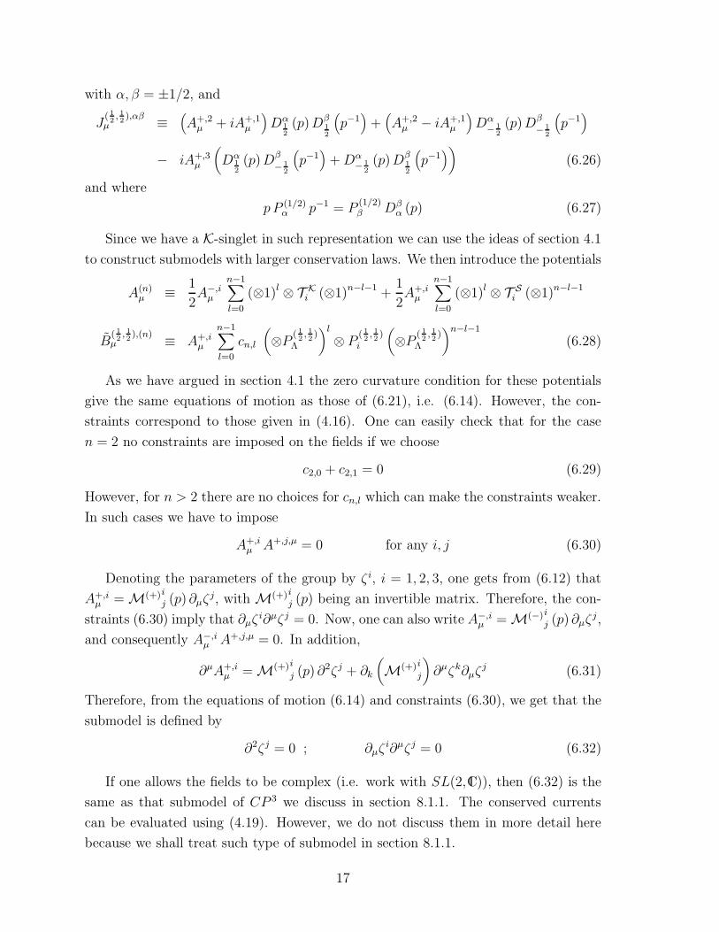
with α, β = ±1/2, and

J( 12, 12),αβ

µ ≡(

A+,2µ + iA+,1

µ

)

Dα1

2

(p)Dβ1

2

(

p−1)

+(

A+,2µ − iA+,1

µ

)

Dα− 1

2

(p)Dβ

− 1

2

(

p−1)

− iA+,3µ

(

Dα1

2

(p)Dβ

− 1

2

(

p−1)

+Dα− 1

2

(p)Dβ1

2

(

p−1)

)

(6.26)

and where

p P (1/2)α p−1 = P

(1/2)β Dβ

α (p) (6.27)

Since we have a K-singlet in such representation we can use the ideas of section 4.1

to construct submodels with larger conservation laws. We then introduce the potentials

A(n)µ ≡ 1

2A−,iµ

n−1∑

l=0

(⊗1)l ⊗ T Ki (⊗1)n−l−1 +

1

2A+,iµ

n−1∑

l=0

(⊗1)l ⊗ T Si (⊗1)n−l−1

B( 12, 12),(n)

µ ≡ A+,iµ

n−1∑

l=0

cn,l

(

⊗P ( 12, 12)

Λ

)l

⊗ P( 12, 12)

i

(

⊗P ( 12, 12)

Λ

)n−l−1

(6.28)

As we have argued in section 4.1 the zero curvature condition for these potentials

give the same equations of motion as those of (6.21), i.e. (6.14). However, the con-

straints correspond to those given in (4.16). One can easily check that for the case

n = 2 no constraints are imposed on the fields if we choose

c2,0 + c2,1 = 0 (6.29)

However, for n > 2 there are no choices for cn,l which can make the constraints weaker.

In such cases we have to impose

A+,iµ A+,j,µ = 0 for any i, j (6.30)

Denoting the parameters of the group by ζ i, i = 1, 2, 3, one gets from (6.12) that

A+,iµ = M(+)i

j (p) ∂µζj, with M(+)i

j (p) being an invertible matrix. Therefore, the con-

straints (6.30) imply that ∂µζi∂µζj = 0. Now, one can also write A−,i

µ = M(−)i

j (p) ∂µζj,

and consequently A−,iµ A+,j,µ = 0. In addition,

∂µA+,iµ = M(+)i

j (p) ∂2ζj + ∂k

(

M(+)i

j

)

∂µζk∂µζj (6.31)

Therefore, from the equations of motion (6.14) and constraints (6.30), we get that the

submodel is defined by

∂2ζj = 0 ; ∂µζi∂µζj = 0 (6.32)

If one allows the fields to be complex (i.e. work with SL(2,C)), then (6.32) is the

same as that submodel of CP 3 we discuss in section 8.1.1. The conserved currents

can be evaluated using (4.19). However, we do not discuss them in more detail here

because we shall treat such type of submodel in section 8.1.1.

17

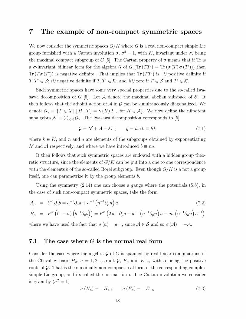
7 The example of non-compact symmetric spaces

We now consider the symmetric spaces G/K where G is a real non-compact simple Lie

group furnished with a Cartan involution σ, σ2 = 1, with K, invariant under σ, being

the maximal compact subgroup of G [5]. The Cartan property of σ means that if Tr is

a σ-invariant bilinear form for the algebra G of G (Tr (TT ′) = Tr (σ (T ) σ (T ′))) then

Tr (Tσ (T ′)) is negative definite. That implies that Tr (TT ′) is: i) positive definite if

T, T ′ ∈ S; ii) negative definite if T, T ′ ∈ K; and iii) zero if T ∈ S and T ′ ∈ K.

Such symmetric spaces have some very special properties due to the so-called Iwa-

sawa decomposition of G [5]. Let A denote the maximal abelian subspace of S. It

then follows that the adjoint action of A in G can be simultaneously diagonalized. We

denote Gγ ≡ T ∈ G | [H , T ] = γ (H)T , for H ∈ A. We now define the nilpotent

subalgebra N ≡ ∑

γ>0 Gγ . The Iwasawa decomposition corresponds to [5]

G = N +A+K ; g = n a k ≡ b k (7.1)

where k ∈ K, and n and a are elements of the subgroups obtained by exponentiating

N and A respectively, and where we have introduced b ≡ na.

It then follows that such symmetric spaces are endowed with a hidden group theo-

retic structure, since the elements of G/K can be put into a one to one correspondence

with the elements b of the so-called Borel subgroup. Even though G/K is a not a group

itself, one can parametrize it by the group elements b.

Using the symmetry (2.14) one can choose a gauge where the potentials (5.8), in

the case of such non-compact symmetric spaces, take the form

Aµ = b−1∂µb = a−1∂µa + a−1(

n−1∂µn)

a (7.2)

Bµ = P ψ(

(1− σ)(

b−1∂µb))

= P ψ(

2 a−1∂µa+ a−1(

n−1∂µn)

a− aσ(

n−1∂µn)

a−1)

where we have used the fact that σ (a) = a−1, since A ∈ S and so σ (A) = −A.

7.1 The case where G is the normal real form

Consider the case where the algebra G of G is spanned by real linear combinations of

the Chevalley basis Ha, a = 1, 2, . . . rank G, Eα and E−α, with α being the positive

roots of G. That is the maximally non-compact real form of the corresponding complex

simple Lie group, and its called the normal form. The Cartan involution we consider

is given by (σ2 = 1)

σ (Ha) = −Ha ; σ (Eα) = −E−α (7.3)

18

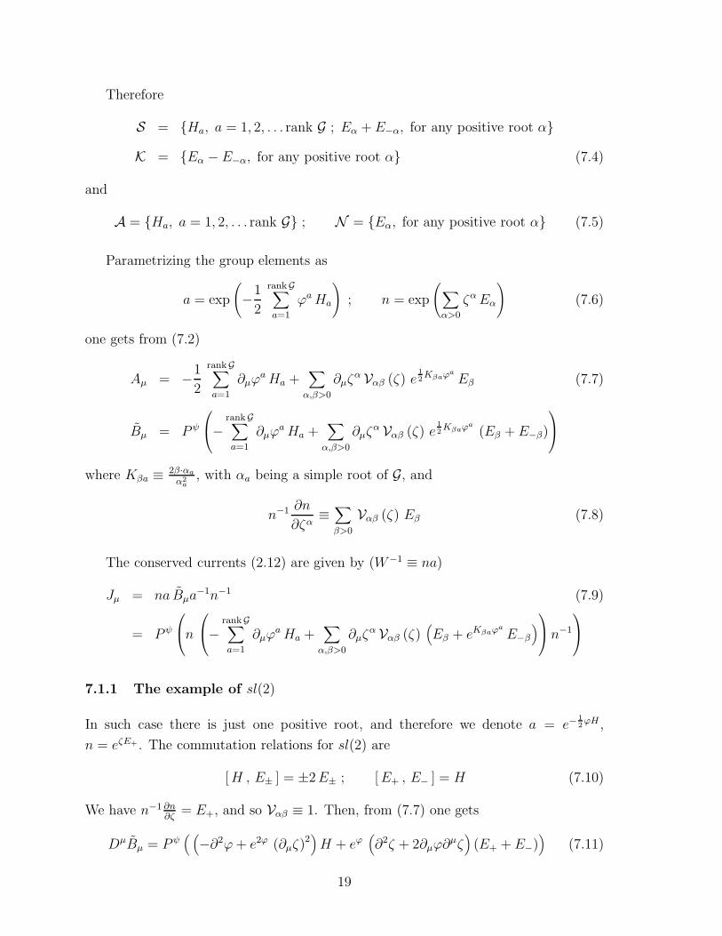
Therefore

S = Ha, a = 1, 2, . . . rank G ; Eα + E−α, for any positive root α

K = Eα − E−α, for any positive root α (7.4)

and

A = Ha, a = 1, 2, . . . rank G ; N = Eα, for any positive root α (7.5)

Parametrizing the group elements as

a = exp

(

−1

2

rankG∑

a=1

ϕaHa

)

; n = exp

(

∑

α>0

ζαEα

)

(7.6)

one gets from (7.2)

Aµ = −1

2

rankG∑

a=1

∂µϕaHa +

∑

α,β>0

∂µζα Vαβ (ζ) e

1

2Kβaϕ

a

Eβ (7.7)

Bµ = P ψ

−rankG∑

a=1

∂µϕaHa +

∑

α,β>0

∂µζα Vαβ (ζ) e

1

2Kβaϕ

a

(Eβ + E−β)

where Kβa ≡ 2β·αa

α2a, with αa being a simple root of G, and

n−1 ∂n

∂ζα≡∑

β>0

Vαβ (ζ) Eβ (7.8)

The conserved currents (2.12) are given by (W−1 ≡ na)

Jµ = na Bµa−1n−1 (7.9)

= P ψ

n

−rankG∑

a=1

∂µϕaHa +

∑

α,β>0

∂µζα Vαβ (ζ)

(

Eβ + eKβaϕa

E−β

)

n−1

7.1.1 The example of sl(2)

In such case there is just one positive root, and therefore we denote a = e−1

2ϕH ,

n = eζE+ . The commutation relations for sl(2) are

[H , E± ] = ±2E± ; [E+ , E− ] = H (7.10)

We have n−1 ∂n∂ζ

= E+, and so Vαβ ≡ 1. Then, from (7.7) one gets

DµBµ = P ψ( (

−∂2ϕ+ e2ϕ (∂µζ)2)

H + eϕ(

∂2ζ + 2∂µϕ∂µζ)

(E+ + E−))

(7.11)

19

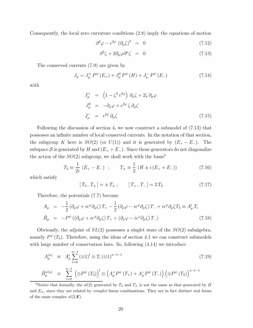
Consequently, the local zero curvature conditions (2.8) imply the equations of motion

∂2ϕ− e2ϕ (∂µζ)2 = 0 (7.12)

∂2ζ + 2∂µϕ∂µζ = 0 (7.13)

The conserved currents (7.9) are given by

Jµ = J+µ P

ψ (E+) + J0µ P

ψ (H) + J−µ P

ψ (E−) (7.14)

with

J+µ =

(

1− ζ2 e2ϕ)

∂µζ + 2ζ ∂µϕ

J0µ = −∂µϕ+ e2ϕ ζ ∂µζ

J−µ = e2ϕ ∂µζ (7.15)

Following the discussion of section 4, we now construct a submodel of (7.13) that

possesses an infinite number of local conserved currents. In the notation of that section,

the subgroup K here is SO(2) (or U(1)) and it is generated by (E+ − E−). The

subspace S is generated byH and (E+ + E−). Since those generators do not diagonalize

the action of the SO(2) subgroup, we shall work with the basis3

T3 ≡1

2i(E+ − E−) ; T± ≡ 1

2(H ± i (E+ + E−)) (7.16)

which satisfy

[T3 , T± ] = ±T± ; [T+ , T− ] = 2 T3 (7.17)

Therefore, the potentials (7.7) become

Aµ = −1

2(∂µϕ+ ieϕ∂µζ)T+ − 1

2(∂µϕ− ieϕ∂µζ)T− + ieϕ∂µζT3 ≡ Aiµ Ti

Bµ = −P ψ ((∂µϕ+ ieϕ∂µζ)T+ + (∂µϕ− ieϕ∂µζ)T−) (7.18)

Obviously, the adjoint of SL(2) possesses a singlet state of the SO(2) subalgebra,

namely P ψ (T3). Therefore, using the ideas of section 4.1 we can construct submodels

with large number of conservation laws. So, following (4.14) we introduce

A(n)µ ≡ Aiµ

n−1∑

l=0

(⊗1)l ⊗ Ti (⊗1)n−l−1 (7.19)

Bψ(n)µ ≡

n−1∑

l=0

(

⊗P ψ (T3))l ⊗

(

A+µP

ψ (T+) + A−µP

ψ (T−)) (

⊗P ψ (T3))n−l−1

3Notice that formally, the sl(2) generated by T3 and T± is not the same as that generated by H

and E±, since they are related by complex linear combinations. They are in fact distinct real forms

of the same complex sl(2,C).

20

According to the comments below (4.4) and (4.14) we could have rescaled the basis of

the irreducible representations of SO(2), independently. However, such freedom would

not produce more submodels with infinite number of conserved currents (see discussion

below (8.33) for a similar situation)4

As we have argued in section 4.1 the zero curvature for these potentials lead to the

equations of motion (7.13) and the constraints corresponding to (4.16). One can verify

that such constraints for any value of n correspond to(

A+µ

)2=(

A−µ

)2= 0, which is

equivalent to

(∂µϕ+ ieϕ∂µζ)2 = 0 (7.20)

Therefore the equations of motion and constraints of the submodel defined by (7.13)

and (7.20) can be written as

∂2ϕ− (∂µϕ)2 = 0 ; ∂2ζ = 0 ; (∂µϕ)

2−e2ϕ (∂µζ)2 = 0 ; ∂µζ∂µϕ = 0 (7.21)

Introducing

φ ≡ e−ϕ ; and so φ ≥ 0 (7.22)

it becomes

∂2φ = 0 ; ∂2ζ = 0 ; ∂µζ∂µφ = 0 ; (∂µφ)

2 = (∂µζ)2 (7.23)

Now, using the results of section 4, we can find an infinite number of conserved

currents for the submodel defined by equations (7.13). These currents will have the

form of (4.19); since for this model

b = na = eζE+ e−1

2ϕH =

e−1

2ϕ ζe

1

2ϕ

0 e1

2ϕ

, (7.24)

the Vα(b)’s take the form

b P ψ (T3) b−1 = P ψ

V 0 V +

V − −V 0

(7.25)

with

V + =(

1 + ζ2e2ϕ)

e−ϕ =

(

1 +ζ2

φ2

)

φ

V 0 = −ζeϕ = − ζφ

V − = −eϕ = −1

φ4There is an additional choice which would lead to the constraint | ∂µϕ+ ieϕ∂µζ |2= 0, instead of

(7.20). However, the method of section 4.1 would lead to conserved currents for the case n = 2 only.

21

So, for the case n = 2 in (4.19), one gets

J2,(+,+)µ ≡ J+

µ V+ = e−ϕ

(

1 + ζ2 e2ϕ) [

2 ζ ∂µϕ+(

1− ζ2 e2ϕ)

∂µζ]

;

J2,(0,0)µ ≡ J0

µ V0 = ζ eϕ ∂µϕ− ζ2 e3ϕ ∂µζ ;

J2,(−,−)µ ≡ J−

µ V− = −e3ϕ ∂µζ ;

J2,(0,−)µ ≡ J0

µ V− + J−

µ V0 = eϕ∂µϕ− 2 ζ e3ϕ ∂µζ ;

J2,(0,+)µ ≡ J0

µ V+ + J+

µ V0 = 2 ζ3 e3ϕ ∂µζ −

(

1 + 3 ζ2 e2ϕ)

e−ϕ ∂µφ ;

J2,(+,−)µ ≡ J+

µ V− + J−

µ V+ = 2 ζ2 e3ϕ ∂µζ − 2 ζ eϕ ∂µϕ ;

The models discussed in section 7.1, and in particular the example of sl(2) given

by (7.13), have been discussed in the literature [9, 10] in the context of dualities in

supergravity theories. It would be interesting to investigate the role of such infinite set

of conserved currents in those theories.

8 The CPN models

The CPN model contains N complex scalar fields ui, i = 1, 2, . . .N , and on a space-time

of d+ 1 dimensions it is defined by the action

S ≡∫

dd+1x

(

1 + u† · u) (

∂µu† · ∂µu

)

−(

u† · ∂µu) (

∂µu† · u)

(1 + u† · u)2(8.1)

where we have denote by u the N -dimensional column matrix with components ui, and

by u† the complex conjugate of its transpose. The corresponding equations of motion

are5(

1 + u† · u)

∂2ui = 2(

u† · ∂µu)

∂µui (8.2)

and the corresponding complex conjugates.

The CPN model corresponds in fact to the non-linear sigma model on the symmetric

space SU(N + 1)/SU(N) × U(1), defined in the manner discussed in section 5, and

therefore possesses a local zero curvature representation as discussed there. See [11, 12]

for alternative formulations. Let αi and λi, i = 1, 2, . . .N , denote the simple roots and

5Actually the equation of motion following from (8.1) is(

1 + u† · u)

∂2ui + 2(u†·∂µu)

2

ui

(1+u†·u) −2(

u† · ∂µu)

∂µui−(

u† · ∂2u)

ui = 0. However, such equation (as well as (8.2)) implies, by contraction

with u∗i , that

(

u† · ∂2u)

= 2(u†·∂µu)

2

(1+u†·u) . Those two relations leads to (8.2).

22

fundamental weights respectively, of SU(N+1). They satisfy2λi·αj

α2j

= δij . The relevant

involutive automorphism is given by

σ (T ) ≡ ΩT Ω−1 ; Ω ≡ eiπΛ ; Λ ≡ 2 λN ·Hα2N

(8.3)

with T being an element of the algebra su(N +1), and Hi being the basis of its Cartan

subalgebra. Therefore, the subalgebra of su(N + 1) invariant under σ is generated

by the Cartan subalgebra and the step operators E±α corresponding to roots which

are orthogonal to λN , or in other words, which do not contain αN in its expansion

in terms of simple roots. Therefore, it corresponds to the subalgebra su(N) ⊕ u(1),

where the simple roots of such su(N) are the first N −1 simple roots of su(N +1), i.e.

αa, a = 1, 2, . . .N − 1. The u(1) factor is obviously generated by Λ defined in (8.3).

Following the notation of (5.1) one has

S ≡ S±i ≡ E±(αi+αi+1+...αN ) ; i = 1, 2, . . .N

K ≡ su(N)⊕ u(1) (8.4)

The action and equations of motion of the CPN model can then be written in the

form (5.4) and (5.5) respectively. The main problem is to find the correct parametriza-

tion in terms of the fields ui of the SU(N + 1) group element g, in (5.3), such that

(5.5) reproduces (8.2). The answer to it is

g = eiS eϕ[S , S† ] eiS

†

; ϕ ≡ log√1 + u† · uu† · u (8.5)

where we have defined

S ≡ ui Si S† ≡ u∗i S−i (8.6)

with S±i introduced in (8.4), and where we have used the fact that in any finite di-

mensional representation we can choose the basis such that H†i = Hi and E

†α = E−α.

In the (N + 1)-dimensional defining representation of SU(N + 1), g is given by

g ≡ 1

ϑ

∆ iu

iu† 1

; ϑ ≡√

1 + u† · u (8.7)

where ∆ is a N ×N hermitian matrix given by

∆ij ≡ ϑ δij −uiu

∗j

1 + ϑ; i, j = 1, 2, . . .N (8.8)

It then follows that g is indeed an unitary matrix.

23

Notice that u is an eigenvector of ∆ with unit eigenvalue

∆ · u = u (8.9)

In the defining representation, Λ and Ω leading to the automorphism σ of (8.3) are

given by

Λ =1

N + 1

1lN×N 0

0 −N

Ω = eiπ/(N+1)

1lN×N 0

0 −1

(8.10)

and therefore6

σ (g) = Ω gΩ−1 = g−1 and y (g) = g2 (8.11)

where y (g) is defined in (5.3).

One can check that

g−1∂µg =1

ϑ2

κµ i∆ · ∂µui(

∂µu†)

·∆ vµ

(8.12)

where

κµij ≡ ϑ

1 + ϑ

(

ui∂µu∗j − (∂µui)u

∗j

)

+1

2

(

u† · ∂µu−(

∂µu†)

· u) uiu

∗j

(1 + ϑ)2

vµ ≡ 1

2

(

u† · ∂µu−(

∂µu†)

· u)

(8.13)

One can write (8.12) as a linear combination of a basis of su(N + 1) using the odd

generators S±i introduced in (8.4). In order to simplify the notation we introduce the

covariant derivative

∇µui ≡ ∆ij∂µuj =

(

ϑ ∂µ −u† · ∂µu1 + ϑ

)

ui (8.14)

The potentials (5.8) can then be written as

Aµ = g−1∂µg

=1

ϑ2

i∇µS + i (∇µS)† +

[

S , (∂µS)†]

−[

∂µS , S†]

1 + ϑ− vµ

[

S , S†]

(1 + ϑ)2

Bµ = P ψ(

(1− σ)(

g−1∂µg))

(8.15)

=2i

ϑ2P ψ

(

∇µS + (∇µS)†)

=2i

ϑ2

(

∇µui Pψ (Si) + (∇µui)

† P ψ (S−i))

6Notice that, from (8.3), (8.5) and (8.11), one has (in the defining representation at least) that

ΩgΩ−1 = e−iS eϕ[S , S† ] e−iS†

= g−1, and so one can also write g = eiS†

e−ϕ[S , S† ] eiS .

24

Notice that in the even part under σ of Aµ, i.e. the terms involving commutators of

S’s, the ordinary derivative can be replaced by the covariant derivatives (8.14) due to

the antisymmetry of the terms.

By imposing the local zero curvature condition (2.8) on these potentials one obtains

the CPN equations of motion (8.2). Indeed, the flatness condition Fµν = 0 is trivially

satisfied since Aµ is of the pure gauge form. The condition DµBµ = 0 leads to 2N

equations which are equivalent to (8.2).

According to (2.12) (or (3.12)) the conserved currents of the CPN model are given

by7

Jµ = g Bµ g−1 = 2P ψ

J ijµ iJ iµiJ iµ

† −Jµ

= P ψ(

J ijµ [Si , S−j ] + iJ iµ Si + iJ iµ†S−i

)

=1

1 + u† · u Pψ([

∂µ(

S + S†)

, S + S†]

+ i∂µ(

S + S†)

− u† · ∂µu− ∂µu† · u

1 + u† · u(

i(

S − S†)

+[

S , S†])

)

(8.16)

with i, j = 1, 2, . . .N , and

J ijµ =

(

1 + u† · u) (

∂µui u†j − ui∂µu

†j

)

− uiu†j

(

u† · ∂µu− ∂µu† · u

)

(1 + u† · u)2

J iµ =

(

1 + u† · u)

∂µui − ui(

u† · ∂µu− ∂µu† · u

)

(1 + u† · u)2

Jµ =u† · ∂µu− ∂µu

† · u(1 + u† · u)2

(8.17)

In (8.16) J ijµ , Jiµ, J

iµ†and Jµ stand for matrices (N × N), (N × 1), (1 × N) and

(1 × 1) respectively. Notice that the number of conserved currents is indeed equal to

the dimension of SU(N + 1), i.e. (N2 + 2N), since∑Ni=1 J

iiµ = Jµ.

7Where we have used the fact that in the defining representation of SU(N + 1), one has (Si)rs =

δirδs,N+1 and (S−i)rs = δr,N+1δis, with r, s = 1, 2, . . .N + 1, and i = 1, 2, . . .N .

25

8.1 Integrable submodels of CPN

We now follow the strategy of section 4 to construct submodels of CPN which presents

an infinite number of conserved currents.

Since su(N + 1) has no roots containing twice ±αN in their expansions in terms

of simple roots, it follows that S defined in (8.4) splits into two abelian subspaces

generated by Si and S−i, i.e.

S = S+ + S− ; S± ≡ S±i ; i = 1, 2, . . .N (8.18)

and

[Si , Sj ] = [S−i , S−j ] = 0 ; any i, j (8.19)

It follows that S+ and S− transform under the representations N(1) and N(−1)

respectively, of the subalgebra K = su(N)⊕ u(1), i.e.

[

K , P ψ (Si)]

= P ψ (Sj) RN(1)ji (K)

[

K , P ψ (S−i)]

= P ψ (S−j) RN(−1)ji (K) (8.20)

Therefore, according to the discussion of section 4 we have to look for representa-

tions P λ of su(N + 1) such that its branching in terms of su(N)⊕ u(1) possesses the

representations N(1) and N(−1) at least once, i.e.

P λ = N(1) + N(−1) + anything (8.21)

If that happens let us denote by P λi and P λ

−i, i = 1, 2, . . .N , the basis of the subspaces

corresponding to N(1) and N(−1) respectively, that transform exactly like P ψ (Si) and

P ψ (S−i), i.e.

[

K , P λi

]

= P λj R

N(1)ji (K)

[

K , P λ−i

]

= P λ−j R

N(−1)ji (K) (8.22)

As we have commented below (4.4), we can rescale the basis P λi and P λ

−i of N(1) and

N(−1) respectively, independently without changing the relation between (8.20) and

(8.22). Then following (8.15), we introduce the potential

Bλµ =

2i

ϑ2

(

∇µui Pλi + β (∇µui)

† P λ−i

)

(8.23)

where β is the parameter accounting for the freedom of rescaling the basis of the

irreducible components.

26

Again, according to the arguments of section 4 the zero curvature condition

Dµ Bλµ = 0 (8.24)

where the covariante derivative is w.r.t. the same potential Aµ as in (8.15), leads to

the equations of motion of the CPN model (8.2) plus the constraints (see (4.7))

∂µui ∂µuj

([

Si , Pλj

]

+[

Sj , Pλi

])

= 0 (8.25)

∂µu∗i ∂

µu∗j([

S−i , Pλ−j

]

+[

S−j , Pλ−i

])

= 0 (8.26)

∂µui ∂µu∗j

(

β[

Si , Pλ−j

]

+[

S−j , Pλi

])

= 0 (8.27)

In the above calculation we have used that ∇µui = ∆ij∂µuj, together with the fact

that ∆ij is invertible, i.e.

∆−1ij ≡ 1

ϑ

(

δij +uiu

∗j

1 + ϑ

)

(8.28)

Therefore, any eq. of the type ∇µui∇µujMij = 0 can be written as ∂µui ∂µujMij = 0,

for a genereic tensor Mij .

We have that the terms involving commutators in (8.25), (8.26), and (8.27) trans-

form under K = su(N) ⊕ u(1) as (N ×N)s (2) = N(N+1)2

(2),(

N × N)

s(−2) =

N(N+1)2

(−2), and(

N × N)

(0) = (1 + adjoint) (0), respectively. Therefore, as we dis-

cussed in section 4, the constraints (8.25)-(8.27) will only be effective if such represen-

tation appear in the branching of P λ in terms of representations of K = su(N)⊕ u(1).

In any case, the model defined by the equations (8.2) and constraints (8.25)-(8.27)

possesses the conserved currents (see (2.12))

Jλµ ≡ g Bλµ g

−1 (8.29)

with g given by (8.5). If the number of representations P λ satisfying the conditions

discussed above is infinite, one obviously gets an infinite number of conserved currents.

8.1.1 The singlet states and infinite number of currents

The adjoint representation of SU(N +1) decomposes into representations of SU(N)⊗U(1) as

Adj (SU(N + 1)) = N(1) + N(−1) + Adj (SU(N)) (0) + 1(0) (8.30)

Therefore it possesses a singlet state satisfying (4.12). That singlet corresponds to the

U(1) generator Λ defined in (8.3) and (8.10).

27

Consequently, we can apply the ideas of section 4.1 to construct an infinite number

of conserved currents for submodels of CPN . Denoting the generators of K = su(N)⊕u(1), by Kr, r = 1, 2, . . .N2, one can write the potential Aµ in (8.15) as

Aµ = i(

ArµKr + bµ + b†µ)

; bµ ≡ ∇µS

1 + u† · u (8.31)

Then, following (4.14) we define

A(n)µ ≡ i

n−1∑

l=0

(⊗1)l ⊗(

ArµKr + bµ + b†µ)

(⊗1)n−l−1 (8.32)

Bψ(n)µ ≡ 2i

n−1∑

l=0

(

⊗P ψ (Λ))l ⊗ P ψ

(

cn,l bµ + cn,l b†µ

) (

⊗P ψ (Λ))n−l−1

Since the representation RS = N(1) + N(−1), is reducible we can rescale each irre-

ducible component independently (see comments below (4.4) and (4.14)). The con-

stants cn,l and cn,l account for such freedom.

We now impose that these potentials should satisfy the zero curvature conditions

(4.8). Obviously A(n)µ satisfy Fµν = 0. As we have argued in section 4.1, the components

of the condition DµBψ(n)µ = 0, involving ∂µBψ(n)

µ and the commutator of Bψ(n)µ with

the K-part of A(n)µ lead to the equations of motion of the CPN model (8.2). The

commutator of Bψ(n)µ with the S-part of A(n)

µ leads to the constraints defining the

submodel. We analyze those constraints by collecting the linearly independent terms

in the tensor product. The terms involving bµ’s in the l and m positions of the tensor

product are (l < m)

(cn,l + cn,m)(

⊗P ψ (Λ))l−1 ⊗ P ψ (bµ)

(

⊗P ψ (Λ))m−l

P ψ (bµ)(

⊗P ψ (Λ))n−m

(8.33)

− (cn,l + cn,l)(

⊗P ψ (Λ))l−1 ⊗ P ψ

(

b†µ) (

⊗P ψ (Λ))m−l

P ψ(

b†µ) (

⊗P ψ (Λ))n−m

− (cn,l − cn,m)(

⊗P ψ (Λ))l−1 ⊗ P ψ (bµ)

(

⊗P ψ (Λ))m−l

P ψ(

b†µ) (

⊗P ψ (Λ))n−m

+ (cn,l − cn,m)(

⊗P ψ (Λ))l−1 ⊗ P ψ

(

b†µ) (

⊗P ψ (Λ))m−l

P ψ (bµ)(

⊗P ψ (Λ))n−m

= 0

where we have used the fact that[

Λ , bµ + b†µ]

= bµ − b†µ.

The terms involving commutators of bµ’s are

(cn,l − cn,l)(

⊗P ψ (Λ))l ⊗ P ψ

([

bµ , b†µ]) (

⊗P ψ (Λ))n−l−1

= 0 (8.34)

Therefore, if we choose

cn,l = cn,l = 1 ; for any n and l (8.35)

28

we get the contraints ∇µui∇µuj = 0 and (∇µui)† (∇µuj)

† = 0, for any i and j.

However, from (8.14) we have that ∇µui = ∆ij∂µuj, and since ∆ij is invertible (see

(8.28)), it follows that the constraints become just ∂µui ∂µuj = 0 and their complex

conjugates. Using such contraints on the equation of motion of CPN (8.2) one gets

that ∂2ui = 0. Consequently, the submodel we obtain is defined by the equations

∂2ui = 0 ; ∂µui ∂µuj = 0 (8.36)

and the corresponding complex conjugate equations.

According to the discussions of section 4.1 such submodel possesses an infinite

number of currents given by (4.19). The quantities Vα, defined in (4.18), are given by

g P ψ (Λ) g−1 = P ψ

V ij −iV i

iV i† −V

= P ψ(

V ij [Si , S−j ]− iV i Si + iV i† S−i

)

= P ψ(

Λ− 1

1 + u† · u([

S , S†]

+ i(

S − S†))

)

(8.37)

with i, j = 1, 2, . . .N , and

V ij ≡ δijN + 1

− uiu†j

1 + u† · uV i ≡ ui

1 + u† · u

V ≡ − 1

N + 1+

1

1 + u† · u (8.38)

In (8.37) we are using the same notation as in (8.16). The number of independent

quantities V ’s is the dimension of SU(N + 1), since∑Ni=1 Vii = V .

One can easily check that the currents (8.17) can be written in terms of (8.38) as

J ijµ = −(

δV ij

δum∂µum − δV ij

δu†m∂µu

†m

)

J iµ =δV i

δum∂µum − δV i

δu†m∂µu

†m

J iµ†

= −

δV i†

δum∂µum − δV i†

δu†m∂µu

†m

(8.39)

Since we have chosen all the cn,l’s to be unity (see (8.35)), it follows that all the

conserved currents (4.19) are of the form

Jα1α2...αn

µ ≡ δFα1α2...αn

δum∂µum − δFα1α2...αn

δu†m∂µu

†m (8.40)

29

where

Fα1α2...αn ≡ −n∏

l=1

V αl (8.41)

with V αl’s being any of the quantities in (8.38), i.e V ij , V i and V i†.

In fact, any quantity of the form

Jµ = Mi∂µui +Ni∂µu†i (8.42)

with Mi and Ni being functionals of uj and u†j, is a conserved current of the submodel

(8.36) provided [12]δMi

δu†j+δNj

δui= 0 (8.43)

The conserved quantitites we have obtained above, using the ideas of section 4.1, are

particular examples of the cases where Mi =δFδui

and Ni = − δF

δu†i

.

It is worth mentioning that the amount of conservation laws the submodel (8.36)

possesses is due (at least partially) to the huge symmetry group it presents. Indeed,

the submodel (8.36) is invariant under the transformations

ui → u′i ≡ ω(1)i (u) + ω

(2)i (u∗)

u∗i → u∗ ′i ≡ ω(1)−i (u) + ω

(2)−i (u

∗) (8.44)

provided

ω(1)i (u)ω

(2)j (u∗) + ω

(2)i (u∗)ω

(1)j (u) = h

(1)ij (u) + h

(2)ij (u∗)

ω(1)−i (u)ω

(2)−j (u

∗) + ω(2)−i (u

∗)ω(1)−j (u) = h

(1)−i,−j (u) + h

(2)−i,−j (u

∗) (8.45)

for any i, j, k, l = 1, 2, . . .N , and where(

ω(1)±i , h

(1)±i,±j

)

and(

ω(2)±i , h

(2)±i,±j

)

are functions of

ui’s and u∗i ’s only, respectively. Particular solutions for (8.45) are obtained by taking

ω(1)i = const., and ω

(2)j arbitrary, or vice-versa. The same being true for the negative

ω’s. Therefore, starting with a suitable small set of currents, a large amount of other

currents can be construct using the transformations (8.44).

30

In the case n = 2, the currents (8.40) are given by

J ijµ Vkl + V ijJklµ =

1

(1 + u† · u)2

2(u† · ∂µu− ∂µu† · u)

1 + u† · u uiu†juku

†l

+(1 + u† · u)(N + 1)

[

δkl(∂µuiu†j − ui∂µu

†j) + δij(∂µuku

†l − uk∂µu

†l )]

− uiu†j(∂µuku

†l − uk∂µu

†l )− uku

†l (∂µuiu

†j − ui∂µu

†j)

− (u† · ∂µu− ∂µu† · u)

N + 1

(

δkluiu†j + δijuku

†l

)

J ijµ Vk − V ijJkµ =

1

(1 + u† · u)2[

uk(

∂µuiu†j − ui∂µu

†j

)

+ uiu†j∂µuk

−2(

u† · ∂µu− ∂µu† · u

)

1 + u† · u ui u†j uk

− 1 + u† · uN + 1

δij∂µuk +(u† · ∂µu− ∂µu

† · u)N + 1

ukδij

]

J iµVj + V iJ jµ =

ui∂µuj + uj∂µui

(1 + u† · u)2− 2uiuj

(1 + u† · u)3(

u† · ∂µu− ∂µu† · u

)

J ijµ Vk† + V ijJkµ

†=

1

(1 + u† · u)2[

u†k(∂µuiu†j − ui∂µu

†j)

− 2(u† · ∂µu− ∂µu

† · u)1 + u† · u uiu

†ju

†k − uiu

†j∂µu

†k

+1 + u† · uN + 1

δij∂µu†k +

(u† · ∂µu− ∂µu† · u)

N + 1δiju

†k

]

J iµ†V j − V i†J jµ =

1

(1 + u† · u)3(

1 + u† · u) (

∂µu†iuj − u†i∂µuj

)

+ 2 u†iuj(

u† · ∂µu− ∂µu† · u

)

(8.46)

J iµ†V j† + V i†J jµ

†=

∂µu†iu

†j + u†i∂µu

†j

(1 + u† · u)2− 2u†iu

†j

(1 + u† · u)3(

∂µu† · u− u† · ∂µu

)

Notice that with the choice (8.35), the operator Bψ(n)µ given in (8.32), belongs to

the symmetric part of the tensor product. Therefore, the above currents are associated

to the irreducible representations of SU(N + 1) in the symmetric part of the tensor

product of the adjoint representation with itself. For instance, in the case of N = 1

one gets that the adjoint (triplet) of SU(2) satisfies 3⊗ 3 = 5s + 3a + 1s. Indeed, for

N = 1 one can easily check that (8.46) gives 6 currents and that 5 of them coincide

31

with the spin j = 2 (5) currents calculated in [4] for the example of CP 1. The sixth

one coincides with one of the spin j = 1 currents of [4].

8.1.2 Further submodels

When analyzing the constraints (8.33) and (8.34) we looked for a solution valid for any

n in order to have an infinite number of currents. However, for the case n = 2 there is

an additional solution, besides (8.35), which corresponds to

c2,0 + c2,1 = 0 ; c2,0 + c2,1 = 0 (8.47)

Such choice leads to the submodel of CPN defined by(

1 + u† · u)

∂2ui = 2(

u† · ∂µu)

∂µui ; ∂µui ∂µu∗j = 0 (8.48)

with i, j = 1, 2, . . .N . Therefore, using the same procedures of section 8.1.1 one obtains

conserved currents of the type (8.46). In such case, the currents will depend upon one

parameter which is the ratio c2,0/c2,0.

Additional conserved currents for the submodel (8.48) can be constructed using the

ideas of section 8.1. As an example consider the case of CP 2. The representations 10

and 10 of SU(3) break into irreducibles of SU(2)⊗ U(1) as

10 = 4(1) + 3(0) + 2(−1) + 1(−2)

10 = 4(−1) + 3(0) + 2(1) + 1(2) (8.49)

Therefore, 10+ 10 contains the representation RS = 2(1)+ 2(−1) discussed in (8.21),

and therefore one can defined an operator Bµ like in (8.23) using such representa-

tions. One can check that the constraints (8.25)-(8.27) can be solved by imposing

∂µui ∂µu∗j = 0, i, j = 1, 2. Then through (8.29) one obtains 20 conserved currents for

the corresponding submodel (8.48) of CP 2. A more careful analysis is necessary to

work out all the conserved currents of such type of submodels.

Acknowledgements

We are grateful to J.A.C. Alcaraz, H. Aratyn, J.F. Gomes and A.H. Zimerman for

interesting discussions. L.A.F. is partially supported by CNPq (Brazil) and E.E.L. is

supported by FAPESP (Brazil).

32

References

[1] N. Seiberg and E. Witten; Nucl. Phys. B426 (1994) 19; hep-th 9407087 Nucl.

Phys. B431 (1994) 484; hep-th 9408099 C. Vafa and E. Witten; Nucl. Phys.

B431 (1994) 3; hep-th/9408074.

[2] C. Montonen and D. Olive; Phys. Lett. 72B (1977) 117; D. Olive; Nucl. Phys.

Proc. Suppl. 45A (1996) 88; hep-th/9508089; L.A. Ferreira, Exact electromagnetic

duality I and D. Olive, Exact electromagnetic duality II, to appear in the Proceed-

ings of the IX Jorge Andre Swieca Summer School, Section: Particles and Fields,

Campos do Jordao, Brazil, Feb/97 (World Scientific)

[3] M. K. Prasad and C. H. Sommerfield; Phys. Rev. Lett. 35 (1975) 760; E. B.

Bogomolny; Sov. J. Nucl. Phys. 24 (1976) 449;

[4] O. Alvarez, L. A. Ferreira and J. Sanchez Guillen, Nucl. Phys. B529 (1998) 689,

hep-th/9710147.

[5] Sigurdur Helgason, Differential Geometry, Lie Groups, and Symmetric Spaces,

Academic Press (1978).

[6] M. Olshanetsky and A. Perelomov, Inventiones Math. 54 (1979) 261; Theor. Math.

Phys. 45 (1980) 843; Phys. Rep. 71 (1981) 313.

[7] H. Eichenherr and M. Forger, Nucl. Phys. B155 (1979) 381; Nucl. Phys. B164

(1980) 528.

[8] D. Gianzo, J.O. Madsen, and J. Sanchez Guillen, Integrable chiral theories in

(2+1)-dimensions; US-FT-3-98; hep-th/9805094, to appear in Nucl. Phys. B

[9] E. Cremmer, I.V. Lavrinenko, H. Lu, C.N. Pope, K.S. Stelle and T.A. Tran;

Euclidean-signature Supergravities, Dualities and Instantons; hep-th/9803259.

[10] E. Cremmer, B. Julia, H. Lu and C.N. Pope; Dualisation of Dualities II: Twisted

self-duality of doubled fields and superdualities; hep-th/9806106.

[11] Kazuyuki Fujii and Tatsuo Suzuki, Non-linear sigma models in (1+2)-dimensions

and an infinite number of conserved currents, hep-th/9802105; Some useful for-

mulas in non-linear sigma models in (1+2)-dimensions, hep-th/9804004; K. Fujii,

Y. Homma and T. Suzuki; Non-linear grassmann sigma models in any dimension

and an infinite number of conserved currents; hep-th/9806084.

33

[12] K. Fujii, Y. Homma and T. Suzuki; Submodels of non-linear grassmann sigma

models in any dimension and conserved currents, exact solutions; hep-th/9809149.

34