arX

iv:h

ep-t

h/96

1119

0v1

24

Nov

199

6

CERN-TH/96-332

hep-th/9611190

Introduction to Seiberg-Witten Theory and its Stringy Origin1

W. Lerche2

CERN, Geneva, Switzerland

We give an elementary introduction to the recent solution of N = 2 supersymmetricYang-Mills theory. In addition, we review how it can be re-derived from string duality.

CERN-TH/96-332

November 1996

1Contribution to the Proceedings of the Spring School and Workshop on String Theory, Gauge Theory and Quantum

Gravity, I.C.T.P., Trieste, Italy, March 18-29, 1996. Based, in part, on lectures given at “Gauge Theories, Applied Super-

symmetry and Quantum Gravity”, Leuven, Summer 1995, and at Les Houches, Summer 1995.2e-mail: lerche@nxth04.cern.ch

1

Introduction to Seiberg-Witten Theory and its Stringy Origin

W. Lerchea

a CERN, Geneva, Switzerland

We give an elementary introduction to the recent solution of N = 2 supersymmetric Yang-Mills theory. In

addition, we review how it can be re-derived from string duality.

1. Introduction

In the last two years, there has been a remark-

able progress in understanding non-perturbative

properties of supersymmetric field and string the-

ories. This dramatic development was initiated

by the work of Seiberg and Witten on N=2 su-

persymmetric Yang-Mills theory [1], and by Hull

and Townsend on heterotic-type II string equiv-

alence [2]. By now, many non-perturbatively ex-

act statements can be made about various types

of supersymmetric Yang-Mills theories with and

without matter, and even more drastic state-

ments about superstring theories in various di-

mensions.

It has become evident that the main insight

is of conceptional nature and goes far beyond

original expectations. The picture that seems

to emerge is that the various known, pertur-

batively defined string theories represent non-

perturbatively equivalent, or dual, descriptions of

one and the same fundamental theory. Moreover,

strings do not appear to play a very privileged

role in this theory, besides higher dimensional p-

branes [3]. It may well turn out, ultimately, that

there is just one theory that is fully consistent at

the non-perturbative level, or a just small num-

ber of such theories. Though the number of free

parameters (“moduli”) may a priori be very large

–which would hamper predictive power– it is clear

that investigating this kind of issues is important

and will shape our understanding of the very na-

ture of grand unification.

A full treatment of these matters is surely out-

side the scope of these lecture notes, and would

be premature anyway. We therefore limit our-

selves to discussing some of the basic concepts,

and since some of these arise already in supersym-

metric Yang-Mills theory, we think it is a good

idea to start in section 2 with a very basic in-

troduction to the original work of Seiberg and

Witten (for gauge group SU(2)). We will em-

phasize the idea of analytic continuation and the

underlying monodromy problem, and show how

the effective action can be explicitly computed.

For other reviews on this subject, see [4].

In section 3 we will then explain the general-

ization to other gauge groups, emphasizing the

role of the “simple singularities” that are canoni-

cally associated with the simply laced Lie groups

of type ADE [5]. The simple singularities will

turn out to be the key to understand how the

SW theory arises in string theory. Indeed, as we

will explain in section 4, the SW theory can ac-

tually be derived from Hull-Townsend string du-

ality. This string duality will also allow to inter-

pret the geometrical structure of the SW theory,

in particular the “auxiliary” Riemann surface, in

concrete physical terms. In section 5, it will turn

out [6] that the SW geometry has indeed a natural

interpretation in terms of a very peculiar string

theory !

2. N = 2 Yang-Mills Theory

2.1. Overview

So, in a nutshell, what is all the excitement

about that has made furor even in the mass me-

2

dia ? As one of the main results one may state

the exact non-perturbative low energy effective

Lagrangian of N=2 supersymmetric Yang-Mills

theory with gauge group SU(2); it contains, in

particular, the effective, renormalized gauge cou-

pling, geff , and theta-angle, θeff :

(θeff(a)

π+

8πi

geff2(a)

)= (2.1)

8πi

g02

︸︷︷︸bare

+2i

πlog[ a2

Λ2

]

︸ ︷︷ ︸one−loop

− i

π

∞∑

ℓ=1

cℓ

(Λ

a

)4ℓ

︸ ︷︷ ︸instanton corrections

Here, Λ is the dynamically generated scale at

which the gauge coupling becomes strong, and

a is the Higgs field. This effective, field depen-

dent coupling arises by setting the renormaliza-

tion scale, µ, equal to the characteristic scale of

the theory, which is given by the Higgs VEV:

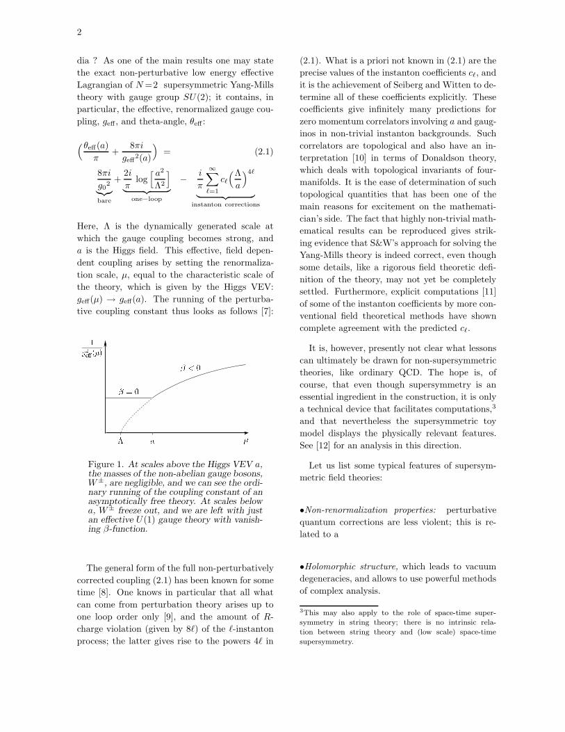
geff(µ) → geff(a). The running of the perturba-

tive coupling constant thus looks as follows [7]:

1g2e()

a = 0 < 0

Figure 1. At scales above the Higgs VEV a,the masses of the non-abelian gauge bosons,W±, are negligible, and we can see the ordi-nary running of the coupling constant of anasymptotically free theory. At scales belowa, W± freeze out, and we are left with justan effective U(1) gauge theory with vanish-ing β-function.

The general form of the full non-perturbatively

corrected coupling (2.1) has been known for some

time [8]. One knows in particular that all what

can come from perturbation theory arises up to

one loop order only [9], and the amount of R-

charge violation (given by 8ℓ) of the ℓ-instanton

process; the latter gives rise to the powers 4ℓ in

(2.1). What is a priori not known in (2.1) are the

precise values of the instanton coefficients cℓ, and

it is the achievement of Seiberg and Witten to de-

termine all of these coefficients explicitly. These

coefficients give infinitely many predictions for

zero momentum correlators involving a and gaug-

inos in non-trivial instanton backgrounds. Such

correlators are topological and also have an in-

terpretation [10] in terms of Donaldson theory,

which deals with topological invariants of four-

manifolds. It is the ease of determination of such

topological quantities that has been one of the

main reasons for excitement on the mathemati-

cian’s side. The fact that highly non-trivial math-

ematical results can be reproduced gives strik-

ing evidence that S&W’s approach for solving the

Yang-Mills theory is indeed correct, even though

some details, like a rigorous field theoretic defi-

nition of the theory, may not yet be completely

settled. Furthermore, explicit computations [11]

of some of the instanton coefficients by more con-

ventional field theoretical methods have shown

complete agreement with the predicted cℓ.

It is, however, presently not clear what lessons

can ultimately be drawn for non-supersymmetric

theories, like ordinary QCD. The hope is, of

course, that even though supersymmetry is an

essential ingredient in the construction, it is only

a technical device that facilitates computations,3

and that nevertheless the supersymmetric toy

model displays the physically relevant features.

See [12] for an analysis in this direction.

Let us list some typical features of supersym-

metric field theories:

•Non-renormalization properties: perturbative

quantum corrections are less violent; this is re-

lated to a

•Holomorphic structure, which leads to vacuum

degeneracies, and allows to use powerful methods

of complex analysis.

3This may also apply to the role of space-time super-

symmetry in string theory; there is no intrinsic rela-

tion between string theory and (low scale) space-time

supersymmetry.

3

•Duality symmetries between electric and mag-

netic, or weak and strong coupling sectors, are

more or less manifest, depending on the number

of supersymmetries.

The maximum number of supersymmetries is four

in a globally supersymmetric theory:

•N=4 supersymmetric Yang-Mills theory is con-

jectured to be self-dual [13], i.e., completely in-

variant under the exchange of electric and mag-

netic sectors. However, though interesting, this

theory is too simple for the present purpose of in-

vestigating non-trivial quantum corrections, since

there aren’t any in this theory.

•N=1 supersymmetric Yang-Mills theory, on the

other hand, is presumably not exactly solvable,

since the quantum corrections are not under full

control; only certain sub-sectors of the theory are

governed by holomorphic objects (like the chiral

superpotential), and thus are protected from per-

turbative quantum corrections. Indeed many in-

teresting results on exact effective superpotentials

have been obtained recently [14].

•N=2 supersymmetric Yang-Mills theory is at the

border between “trivial” and “not fully solvable”,

in that it is in the low-energy limit exactly solv-

able. It is governed by a holomorphic function,

the “prepotential” F , for which the perturbative

quantum corrections are under complete control,

ie., occur just to one loop order.

Having motivated why it is particularly fruitful

to study N = 2 Yang-Mills theory, we now turn

to discuss it in more detail.

2.2. The Semi-Classical Theory for G =

SU(2)

The fields of pure N=2 Yang-Mills theory are

vector supermultiplets in the adjoint representa-

tion of the gauge group. For convenience, one

often rewrites such multiplets in terms of N = 1

chiral multiplets, W iα,Φ

i, as follows:

spin

Aiµ 1

. ..

λiα ψβi 1

2

ւ . ..

W iα φi 0

ւΦi

The bottom component, the scalar field φ ≡ φiσi,

has the following potential:

V (φ) = Tr[φ, φ†]2 . (2.2)

This potential displays a typical feature of super-

symmetric theories, namely flat directions along

which V (φ) ≡ 0. That is, field configurations

φ = a σ3 (2.3)

do not cost any energy. Of course, if a 6= 0, there

is a spontaneous symmetry breakdown: SU(2) →U(1). A more suitable “order” parameter is given

by the gauge invariant Casimir

u(a) = Trφ2 = 2a2 . (2.4)

It is in particular invariant under the Weyl group

of SU(2), which acts as a → −a and is, physi-

cally, the discrete remnant of the gauge transfor-

mations. that act within the Cartan subalgebra.

The quantity u represents a good coordinate of

the manifold Mc of inequivalent vacua, which one

usually calls “moduli space”. Since u can be any

complex number, the moduli space is given by the

complex plane, which may be compactified to the

Riemann sphere by adding a point at infinity.

In the bulk of Mc one has an unbroken U(1)

gauge symmetry, which is enhanced to SU(2) just

at the origin. What we are after is a “Wilso-

nian” effective lagrangian description of the the-

ory, for any given value of u. Such an effective

lagrangian can in principle be obtained by inte-

grating out all fluctuations above some scale µ

4

(that, as we have indicated earlier, is chosen to

be equal to a). In particular, we would integrate

out the massive non-abelian gauge bosonsW±, to

obtain an effective action that involves only the

neutral gauge multiplet, W 0 = (A ≡ Φ0,W 0λ). It

is clear that, semi-classically, this theory can pos-

sibly be meaningful only outside a neighborhood

of u = 0, since at u = 0 the non-abelian gauge

bosonsW± become massless, and the effective de-

scription in terms of only W 0 cannot be accurate

– actually, it would become meaningless. This

tells that u = 0 will be a singular point on Mc

(besides the point of infinity). In order to have a

well-defined theory near u = 0, one would need

to include the charged W -bosons in the effective

theory; one then says that the gauge bosons W±

“resolve” the singularity.

It is clear from Fig.1 that, because of asymp-

totic freedom, the region near u = ∞ will cor-

respond to weak coupling, so that only in this

“semi-classical” region reliable computations can

be done in perturbation theory. On the other

hand, the theory will be strongly coupled near the

classical SU(2)-enhancement point u = 0, so that

a priori no reliable quantum statements about the

theory can be made here.

It is known (just from supersymmetry) that the

low energy effective lagrangian4 is completely de-

termined by a holomorphic prepotential F and

must be of the form:

L =1

4πIm[ ∫

d4θK(A, A)

+

∫d2θ

(12

∑τ(A)WαWα

)]. (2.5)

Here, Φ ≡: Aσ3, and

K(A, A) =∂F(A)

∂AA (2.6)

4By this we mean the piece of the effective lagrangian

that is leading for vanishing momenta, i.e., that contains

at most two derivatives. There are of course infinitely

many higher derivative terms in the full effective action.

These are not governed by holomorphic quantities, and

thus we do not have much control of them. See [15] for

some results in this direction.

is the “Kahler potential” which gives a supersym-

metric non-linear σ-model for the field A, and

τ(A) =∂2F(A)

∂2A. (2.7)

That is, the bosonic piece of (2.5) is, schemati-

cally,

L = Im(τ)∂a ∂a+F ·F

+Re(τ)F ·F +. . . , (2.8)

from which we see that

τ(a) ≡ θ(a)

π+

8πi

g2(a)(2.9)

represents the complexified effective gauge cou-

pling, and Im(τ) is the σ-model metric on Mc.

Classically, F(A) = 12τ0A

2, where τ0 is the bare

coupling constant. However, the full quantum

prepotential will receive [9] perturbative (one-

loop) and non-perturbative corrections, and must

be of the form [8]:

F(A) = (2.10)

1

2τ0A

2 +i

πA2 log

[A2

Λ2

]+

1

2πiA2

∞∑

ℓ=1

cℓ

(Λ

A

)4ℓ

.

By taking two derivatives, F gives rise to the ef-

fective coupling (2.1) mentioned in the introduc-

tion. Note that indeed for large a ≡ A|θ=0, the

instanton sum converges well, and the theory is

dominated by semi-classical, one-loop physics.

A crucial insight [1] is that the global properties

of the effective gauge coupling τ(a) are very im-

portant. Specifically, we know that near u = ∞:

τ = const +2i

πlog[ uΛ2

]+ single valued. (2.11)

This implies that if we loop around u = ∞ in

the moduli space, the logarithm will produce an

extra shift of 2πi because of its branch cut, and

thus:

τ −→ τ − 4 . (2.12)

5

From (2.9) it is clear that this monodromy just

corresponds to an irrelevant shift of the θ-angle,

but what we learn is that τ , as well as F , are not

functions but rather multi-valued sections. Actu-

ally, the full story is more complicated than that,

in that also the imaginary part, Imτ = 8πg2 , will

be globally non-trivial.

More specifically, we see from (2.8) that Im(τ)

represents a metric on the moduli space, and the

physical requirement of unitarity implies that it

must be positive throughout the moduli space:

Im(τ(u)) > 0 . (2.13)

It is now a simple mathematical fact that since

Im(τ) is a harmonic function (ie., ∂∂Im(τ) = 0),

it cannot have a minimum if it is globally defined.

Thus, in order not to conflict with unitarity, we

learn that Im(τ) can only be locally defined –

a priori, it is defined only in the semi-classical

coordinate patch near infinity, cf., (2.11). We

thus conclude that the global structure of the true

”quantum” moduli space, Mq, must be very dif-

ferent as compared to the classical moduli space,

Mc. In particular, any situation with just two

singularities must be excluded.

2.3. The exact quantum moduli space

The question thus arises, how many and what

kind of singularities the exact quantum moduli

space should have, and what the physical signifi-

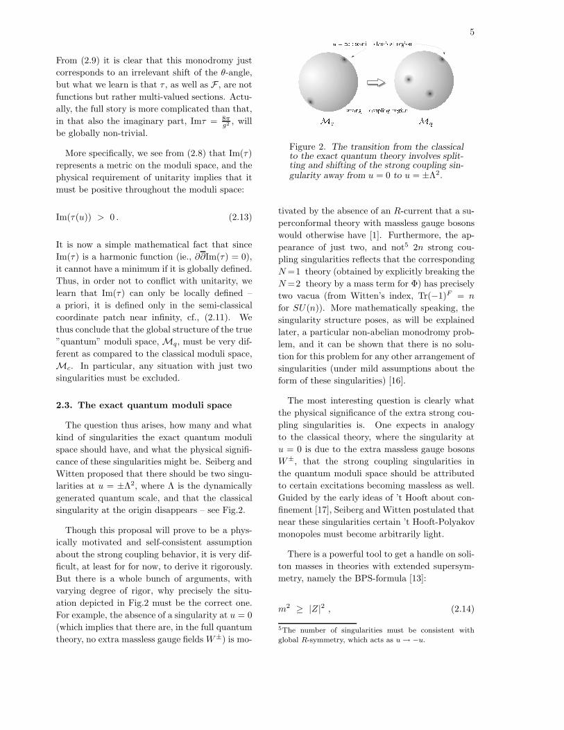
cance of these singularities might be. Seiberg and

Witten proposed that there should be two singu-

larities at u = ±Λ2, where Λ is the dynamically

generated quantum scale, and that the classical

singularity at the origin disappears – see Fig.2.

Though this proposal will prove to be a phys-

ically motivated and self-consistent assumption

about the strong coupling behavior, it is very dif-

ficult, at least for for now, to derive it rigorously.

But there is a whole bunch of arguments, with

varying degree of rigor, why precisely the situ-

ation depicted in Fig.2 must be the correct one.

For example, the absence of a singularity at u = 0

(which implies that there are, in the full quantum

theory, no extra massless gauge fields W±) is mo-

Mc Mqstrong coupling region

u =1 : semi classical region

Figure 2. The transition from the classicalto the exact quantum theory involves split-ting and shifting of the strong coupling sin-gularity away from u = 0 to u = ±Λ2.

tivated by the absence of an R-current that a su-

perconformal theory with massless gauge bosons

would otherwise have [1]. Furthermore, the ap-

pearance of just two, and not5 2n strong cou-

pling singularities reflects that the corresponding

N=1 theory (obtained by explicitly breaking the

N=2 theory by a mass term for Φ) has precisely

two vacua (from Witten’s index, Tr(−1)F = n

for SU(n)). More mathematically speaking, the

singularity structure poses, as will be explained

later, a particular non-abelian monodromy prob-

lem, and it can be shown that there is no solu-

tion for this problem for any other arrangement of

singularities (under mild assumptions about the

form of these singularities) [16].

The most interesting question is clearly what

the physical significance of the extra strong cou-

pling singularities is. One expects in analogy

to the classical theory, where the singularity at

u = 0 is due to the extra massless gauge bosons

W±, that the strong coupling singularities in

the quantum moduli space should be attributed

to certain excitations becoming massless as well.

Guided by the early ideas of ’t Hooft about con-

finement [17], Seiberg and Witten postulated that

near these singularities certain ’t Hooft-Polyakov

monopoles must become arbitrarily light.

There is a powerful tool to get a handle on soli-

ton masses in theories with extended supersym-

metry, namely the BPS-formula [13]:

m2 ≥ |Z|2 , (2.14)

5The number of singularities must be consistent with

global R-symmetry, which acts as u → −u.

6

where Z is the central charge of the superal-

gebra in question. For N = 2 supersymme-

try, this formula immediately follows from uni-

tarity (QQ > 0), in combination with the anti-

commutator

Qαi, Qβj

= δijγ

µαβPµ + δαβǫijU + (γ5)αβǫijV,

where |Z|2 ≡ U2 + V 2. The important point is

that the BPS bound (2.14) is saturated by a cer-

tain class of excitations, namely by the “BPS-

states” that obey Q|ψ〉 = 0. The idea is that

if a state obeys this condition semi-classically,

it obeys it also in the exact quantum theory.

This is because the number of degrees of freedom

of a “short” (or “chiral”) multiplet that obeys

Q|ψ〉 = 0 is smaller as compared to those of a

generic supersymmetry multiplet, and the num-

ber of degrees of freedom is supposed not to jump

when switching on quantum corrections. In par-

ticular, since ’t Hooft-Polyakov monopoles do sat-

isfy the BPS bound semi-classically, they must

obey it in the exact theory as well. From semi-

classical considerations we can also learn that the

monopoles lie in N = 2 hypermultiplets, which

have maximum spin 12 .

For N = 2 supersymmetric Yang-Mills theories,

the central charge takes the form

Z = q a+ g aD , (2.15)

where (g, q) are the (magnetic,electric) quantum

numbers of the BPS state under consideration.

Above, aD is the “magnetic dual” of the elec-

tric Higgs field a and belongs to the N = 2 vec-

tor multiplet (AD,Wα,D) that contains the dual,

magnetic photon, AµD. By studying the electric-

magnetic duality transformation, under which the

ordinary electric gauge potential Aµ transforms

into AµD, it turns out [1] that in the N=2 Yang-

Mills theory the dual variable aD is simply given

by:

aD =∂

∂aF(a) . (2.16)

The general idea is that at the singularity at

u = Λ2, one would have a 6= 0 but aD = 0, such

that (by (2.15)) a monopole hypermultiplet with

charges (g, q) = (±1, 0) would be massless. On

the other hand, one would have that in the exact

theory u = 0 does not imply a = 0, so that in

contrast to the classical theory, no gauge bosons

(with charges (0,±2)) become massless. This in

particular would imply that the classical relation

u = 2a2 can hold only asymptotically in the weak-

coupling region.

The point is to view aD(u) as a variable that is

on a equal footing as a(u); it just belongs to a dual

gauge multiplet that couples locally to magneti-

cally charged excitations, in the same way that

a couples locally to electric excitations (such as

W±). A priori, it would not matter which vari-

able we use to describe the theory, and which

variable we actually use will rather depend on the

region of Mq that we are looking at. More specif-

ically, in the original semi-classical, “electric” re-

gion near u = ∞, the preferred local variable is a,

and an appropriate lagrangian is given by (2.11).

As mentioned above, the instanton sum converges

well for large a ≃√u/2.

However, if we try to extend F(a) to a region

far enough away from u = ∞, we will leave the

domain of convergence of the instanton sum, and

we cannot really make any more much sense of

F . That is, in attempting to globally extend the

effective lagrangian description outside the semi-

classical coordinate patch, we face the problem of

suitably analytically continuing F . The point is

that even though we cannot have a choice of Fthat would be globally valid anywhere on Mq (it

would be in conflict with positivity, cf., (2.13)),

we can resum the instanton terms in F in terms

of other variables, to yield another form of the

lagrangian that converges well in another region

of Mq.

The reader might already have guessed that

while a is the preferred variable near u = ∞, it

is aD that is the preferred variable in the “mag-

netic” strong coupling coordinate patch centered

at u = Λ2. More precisely, near u = Λ2 we expect

to have the following, dual form of the effective

lagrangian:

7

FD(aD) =1

2τD0 aD

2 − i

4πaD

2 log[aD

Λ

]

− 1

2πiΛ2

∞∑

ℓ=1

cDℓ

( iaD

Λ

)ℓ

. (2.17)

The infinite sum indeed converges well, because

at this singularity aD → 0.

From the coefficient of the logarithm we see

that the theory is non-asymptotically free (pos-

itive β-function), and thus weakly coupled for

aD → 0 (though strongly coupled in terms of

the original variable, a). Indeed the dual theory

is simply given by an abelian U(1) gauge theory

(contributing zero to the β-function), coupled to

charged matter that is integrated out (and that

would be massless at aD = 0). The magnitude of

the coefficient shows that there should be a sin-

gle matter field with unit charge coupling to the

(dual) photon, which belongs to a N =2 hyper-

multiplet. This extra matter hypermultiplet is

just the dual representative of the massless mag-

netic monopole. To the dual magnetic photon

related to aD, the monopole looks like an ordi-

nary, elementary (local) field, in spite of that it

couples to the original electric photon in a non-

local way. It is this dual, abelian reformulation of

the original non-abelian instanton problem what

leads to substantial simplifications, especially to

the mathematician’s profit.

Note that the infinite sum of correction terms

in (2.17) reflects the effect of integrating out in-

finitely many massive BPS states, and though its

physical meaning is completely different, has the

same information content as the instanton sum in

the original lagrangian, (2.11). Note also that the

situation at the other singularity, u = −Λ2, does

not present anything new, in that (by u → −usymmetry) it is isomorphic to the the situation

at u = Λ2 and related to it by simply replacing

aD in FD(aD) by aD−2a. The whole scheme can

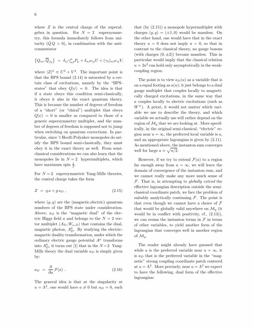
therefore be depicted as in Fig.3.

The alert reader might have noticed that so far

nothing concrete was achieved yet – instead, we

have introduced another set of infinitely many un-

MqF(a) = ia2 log a22 + a22i 1X=1 c`a 4`

FD(aD) = aD24i log aD 22i 1X=1 cD iaD `

~FD = FD(a 2aD)

Figure 3. The exact quantum moduli spaceis covered by three distinct regions, in thecenter of each of which the theory is weaklycoupled when choosing suitable local vari-ables. A local effective lagrangian exists ineach coordinate patch, representing a par-ticular perturbative approximation. Noneof such lagrangians is more fundamentalthan the other ones, and no local lagrangianexists that would be globally valid through-out the moduli space.

knowns, cDℓ – and also that we have just guessed

the coefficient of the logarithm in (2.17). Indeed,

this specific coefficient cannot be derived at this

point, but rather is part of the assumption that a

single monopole with unit charge becomes mass-

less at u = Λ2.

The issue is now to determine the values of all

the unknown coefficients in F , FD (2.11),(2.17)

from the assumptions that govern the local, i.e.,

perturbative behavior of the theory in each of the

three coordinate patches in Fig.3. The local be-

havior is determined by the coefficients of the log-

arithms, which can reliably be computed in one-

loop perturbation theory and directly reflect the

charge quantum numbers of the fields that are

supposed to be light near a given singularity.

The key idea is that it is the patching together

of the known local data in a globally consistent

way that will completely fix the theory (up to

irrelevant ambiguities like θ-shifts). More pre-

cisely, the one-loop term determines the local

monodromy M around a given singularity, and

this acts on the section (aD

a ) as follows:

(aD(u)

a(u)

)−→ M

(aD(u)

a(u)

). (2.18)

In particular, from our knowledge of the asymp-

totic behavior of aD(u), a(u) at semi-classical in-

8

finity,

(aD(u)

a(u)

)≃( i

π

√2u log(u/Λ2))√

u/2

)(2.19)

we infer that for a loop around u = ∞:

M∞ =

(−1 4

0 −1

). (2.20)

As for the strong coupling singularities at u =

±Λ2, we choose a different strategy: we know on

general grounds that the monodromy of a dyon

with charges (g, q) that becomes massless at a

given singularity is given by:

M (g,q) =

(1 + qg q2

−g2 1 − gq

)(2.21)

This can be seen in various ways, one of which

will be explained further below.

The global consistency condition on how to

patch together the local, perturbative data is then

simply

M+Λ2 ·M−Λ2 = M∞ , (2.22)

since we can smoothly pull the monodromy paths

γ around the Riemann sphere (u0 is an arbitrary

base point):

u02 +2 1 +2 2

Figure 4. Monodromy paths in the u-plane.

One may view equation (2.22) as a condition

on the possible massless spectra at u = ±Λ2. For

matrices of the restricted form (2.21), its solution

is:

M+Λ2 = M (1,0)

M−Λ2 = M (1,−2) , (2.23)

which is unique up to irrelevant conjugacy.

From this we can read off the allowed (mag-

netic, electric) quantum numbers of the massless

monopoles/dyons. They indeed give back the co-

efficient of the logarithmic term of FD that we

had anticipated in eq. (2.17).

If we would consider a situation with more than

two strong coupling singularities, we would have

to solve an equation like (2.22) with the corre-

sponding product of matrices (2.21). However, it

can be deduced [16] that such equations for more

than two such matrices do not have any solution.

2.4. Solving the monodromy problem

The physics problem has now become a math-

ematical one, namely simply to find multi-valued

functions a(u), aD(u) that display the required

monodromies M±Λ2,∞ around the singularities

(and that in addition lead to a coupling τ ≡ ∂aaD

with Imτ > 0). This is a classical mathematical

problem, the “Riemann-Hilbert” problem, which

is known to have a unique6 solution.

The RH problem can be accessed from two

complementary point of views: either by consid-

ering a, aD as solutions of a differential equation

with regular singular points, or from considering

a, aD as certain period integrals related to some

auxiliary “spectral surface” X . The latter ap-

proach, to be discussed momentarily, allows an

easy geometric implementation of the right mon-

odromy properties, while the differential equation

approach, to be considered later, is more use-

ful for obtaining explicit expressions for a(u) and

aD(u).

Any two of the monodromy matrices M±Λ2,∞generate the monodromy group ΓM , which con-

stitutes the subgroup Γ0(4) of the modular group

SL(2,ZZ) and consists of matrices of the form

Γ0(4) =( a b

c d

)∈ SL(2,ZZ), b = 0 mod 4

.

6Unique up to multiplication of(

aDa

)(u) by an entire

function; this can however be fixed by imposing the cor-

rect, semi-classical asymptotic behavior.

9

Mathematically speaking, the quantum moduli

space can thus be viewed as the upper half-plane

modulo the monodromy group:

Mq∼= H+

/Γ0(4) . (2.24)

This group represents the quantum symmetries

of the theory, and acts (because of (2.18)) on the

gauge coupling τ = ∂aD(u)∂a(u) via τ → aτ+b

cτ+d . Is

particular, we see that S : τ → − 1τ is not part of

ΓM , and this means that the theory is not weak-

string coupling duality invariant (in contrast to

N=4 Yang-Mills theory).

Now, motivated by the appearance of a sub-

group of the modular group (which is the group of

the discontinuous reparametrizations of a torus),

the basic idea is that the monodromy problem

can be formulated in terms of a toroidal Riemann

surface, whose moduli space is precisely Mq [1].

Such an elliptic curve indeed exists and can be

algebraically characterized by: 7

X1 : y2(x, u) = (x2 − u)2 − Λ4

≡ :

4∏

i=1

(x− ei(u,Λ)) . (2.25)

The point is to interpret the gauge coupling τ(a)

as the period “matrix” of this torus, and this has

the added bonus that manifestly Im(τ) > 0 is

guaranteed, by virtue of a mathematical theorem

called “Riemann’s second relation”. As such is τ

defined by a ratio of period integrals:

τ(u) =D(u)

(u), (2.26)

where

D(u) =

∮

β

ω , (u) =

∮

α

ω (2.27)

with the holomorphic differential ω ≡ 1√2π

dxy(x,u) .

Here, α, β are canonical basis homology cycles of

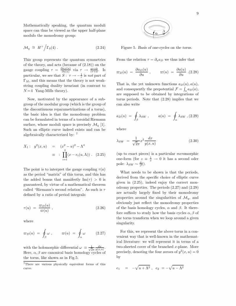
the torus, like shown as in Fig.5.

7There are various physically equivalent forms of this

curve.

Figure 5. Basis of one-cycles on the torus.

From the relation τ = ∂aaD we thus infer that

D(u) =∂aD(u)

∂u, (u) =

∂a(u)

∂u.(2.28)

That is, the yet unknown functions aD(u), a(u),

and consequently the prepotential F =∫

aaD(a),

are supposed to be obtained by integrations of

torus periods. Note that (2.28) implies that we

can also write

aD(u) =

∮

β

λSW , a(u) =

∮

α

λSW , (2.29)

where

λSW =1√2πx2 dx

y(x, u)(2.30)

(up to exact pieces) is a particular meromorphic

one-form (for z ≡ 1x → 0 it has a second oder

pole: λSW ∼ dzz2 ).

What needs to be shown is that the periods,

derived from the specific choice of elliptic curve

given in (2.25), indeed enjoy the correct mon-

odromy properties. The periods (2.27) and (2.29)

are actually largely fixed by their monodromy

properties around the singularities of Mq, and

obviously just reflect the monodromy properties

of the basis homology cycles, α and β. It there-

fore suffices to study how the basis cycles α, β of

the torus transform when we loop around a given

singularity.

For this, we represent the above torus in a con-

venient way that is well-known in the mathemat-

ical literature: we will represent it in terms of a

two-sheeted cover of the branched x-plane. More

precisely, denoting the four zeroes of y2(x, u) = 0

by

e1 = −√u+ Λ2 , e2 = −

√u− Λ2

10

Figure 6. Representation of the auxiliaryelliptic curve X1 in terms of a two-sheetedcovering of the branched x-plane. The twosheets are meant to be glued together alongthe cuts that run between the branch pointsei(u). Shown is our choice of homology ba-sis, given by the cycles α, β. This picturecorresponds to the choice of the basepointu0 > Λ2 real.

e3 =√u− Λ2 , e4 =

√u+ Λ2 , (2.31)

we can specify the torus in the way depicted in

Fig.6.

The singularities in the quantum moduli space

arise when the torus degenerates, and this obvi-

ously happens when any two of the zeros ei co-

incide. This can be expressed as the vanishing of

the “discriminant”

∆Λ =

4∏

i<j

(ei − ej)2 = (2Λ)8(u2 − Λ4) . (2.32)

The zeroes of ∆Λ describe the following degener-

ations of the elliptic curve:

i+) u→ +Λ2, for which (e2 → e3), i.e., the cycle

ν+Λ2 ≡ β degenerates,

i−) u→ −Λ2, for which (e1 → e4), i.e., the cycle

ν−Λ2 ≡ β − 2α degenerates,

ii) Λ2/u→ 0, for which (e1 → e2) and (e3 → e4).

Is is now easy to see that a loop γ+Λ2 around

the singularity at u = Λ2 makes e2 and e3 ro-

tate around each other, so that the cycle α gets

transformed into α−β, as can be seen from Fig.7.

This means that on the basis vector (βα ), the mon-

odromy action looks

(1 0

−1 1

)≡ M (1,0) = M+Λ2 . (2.33)

Similarly, from Fig.7 one can see that the mon-

Figure 7. Vanishing cycles on the torus thatshrink to zero as one moves towards a de-generation point.

odromy around u = −Λ2 is given by

(−1 4

−1 3

)≡ M (1,−2) = M−Λ2 . (2.34)

To obtain the monodromy around Λ2/u→ 0, one

can compactify the u−plane to IP1, as we did be-

fore, and get the monodromy at infinity from the

global relation M∞ = M+Λ2M−Λ2 (cf., Fig.4.).

We thus have reproduced the monodromy ma-

trices associated with the exact quantum moduli

space directly from the the elliptic curve (2.25),

and what this means is that the integrated torus

periods aD(u), a(u) defined by (2.28) must indeed

have the requisite monodromy properties. How-

ever, before we are going to explicitly determine

these functions in the next section, let us say some

more words on the general logic of what we have

just been doing.

We have seen in Fig.7 that when we loop

around a singularity in Mq, the branch points

ei(u) exchange along certain paths, ν, which

shrink to zero as ei → ej . Such paths are called

“vanishing cycles” and play, as we will see, an

important role for the properties of BPS states.

Indeed, in a quite general context, many features

of a BPS spectrum can be encoded in the singular

homology of an appropriate auxiliary surface X .

Concretely, assume that a path vanishes at a

singularity that has the following expansion in

terms of given basis cycles:

ν = g β + q α . (2.35)

Then obviously, assuming that λ does not blow

11

up, we have

0 =

∮

ν

λ = g

∮

β

λ+ q

∮

α

λ = g aD + q a ≡ Z,

so that we have at the singularity a massless BPS

state with (magnetic,electric) charges equal to

(g, q). That is, we can simply read off the quan-

tum numbers of massless states from the coordi-

nates of the vanishing cycle ! Obviously, under

a change of homology basis, the charges change

as well, but this is nothing but a duality rota-

tion. What remains invariant is the intersection

number

νi νj = νt · Ω · ν = giqj − gjqi ∈ ZZ , (2.36)

where is the intersection product of one-cycles

and Ω is the symplectic (skew-symmetric) inter-

section metric for the basis cycles. Note that this

represents the well-known Dirac-Zwanziger quan-

tization condition for the possible electric and

magnetic charges, and we see that it is satisfied by

construction. The vanishing of the r.h.s. of (2.36)

is required for two states to be local with respect

to each other [17,18]. This means that only states

that are related to non-intersecting vanishing cy-

cles are mutually local. In our case, the monopole

with charges (1, 0), the dyon with charges (1,−2)

and the (massive) gauge boson W+ with charges

(0, 2) are all mutually non-local, and thus can-

not be simultaneously represented in a local la-

grangian.

Furthermore, there is a closed formula for the

monodromy around a given singularity associated

with a vanishing cycle: the monodromy action on

any given cycle, γ ∈ H1(X,ZZ), is directly deter-

mined in terms of this vanishing cycle ν by means

of the “Picard-Lefshetz” formula [5]:

Mν : γ −→ γ − (γ ν) ν . (2.37)

This implies that for a vanishing cycle of the form

(2.35), the monodromy matrix is precisely the one

given in (2.21), as promised.

2.5. The BPS Spectrum

We noted above that the global consistency

relation (2.22) is solved by monodromy matri-

ces that correspond to a monopole with charges

(g, q) = ±(1, 0) and to a dyon with charges

±(1,−2). These excitations are massless at u =

Λ2 and u = −Λ2, respectively. We now like to ask

about other BPS states that may exist, though

these must be massive throughout the moduli

space.

For this, remember that the charge labels (g, q)

are highly ambiguous, because they are defined

only up to symplectic transformations; this re-

flects the choice of homology basis. The charges

can thus be changed by conjugation by any mon-

odromy transformation belonging to Γ0(4). In

particular, looping around u = ∞ acts as

M∞ ·M (g,q) ·M∞−1 = M (−g,−q−4g) , (2.38)

and thus will shift the electric charge, q → −q −4g. This corresponds to τ → τ − 4 and to θ →θ − 4π, and hence is a manifestation of the fact

[19] that the electric charge of a dyon changes

if the θ-angle is changed – there is no absolute

definition of the electric charge of a dyon.

It also means that the weak coupling spec-

trum of the theory must be invariant under shifts

θ → θ − 4πn, n ∈ ZZ. That is, under “spectral

flow” induced by smoothly changing θ by 4π, the

BPS spectrum must map back to itself, though in-

dividual states need not map back to themselves.

More precisely, since the above monodromy con-

jugation can be induced by arbitrarily small loops

around u = ∞, we know that the BPS spectrum

should consist in the weak coupling patch at least

of dyons with charges ±(1, 2ℓ), ℓ ∈ ZZ, besides the

massive gauge bosons W± ∼ (0,±2).

A very important point made in [1] is that the

stable BPS spectrum in the strong coupling re-

gion is, in fact, different and consists only of a

subset of the above semi-classical BPS spectrum.

This is because the moduli space Mq decomposes

into two regions, Mweakq and Mstrong

q , with differ-

ent physics. They are separated by a line C, on

which most of the semi-classical BPS states decay.

12

This line is defined by

C =u :

aD(u)

a(u)∈ IR

, (2.39)

and turns out the be almost an ellipse passing

through the singular points at u = ±Λ2; see Fig.8.

Indeed all possible singularities associated with

massless BPS states must lie on C, since if Z =

gaD + qa = 0 for g, q ∈ ZZ, then aD/a ∈ IR.

Figure 8. The line C of marginal stabilityseparates the strong coupling BPS spectrumfrom the semi-classical BPS spectrum. Bothspectra are indicated here by the charges ofthe stable states. The dashed line representsthe logarithmic branch cut.

One can check [20] that if one traces C clockwise

starting from u = −Λ2, (aD/a)(u) varies mono-

tonically from −2 to +2, with (aD/a)(Λ2) = 0.

That we do not map back to (aD/a) = −2 is due

to the branch cut of the logarithm in a(u). Thus

there is really an ambiguity in the electric charge

of the dyon: if we approach u = −Λ2 from the

upper-half u-plane, the dyon has charges ±(1, 2),

which is M∞-conjugate to ±(1,−2) that we had

before.

The physical significance of the marginal line

of stability C is that when (aD/a)(u) ∈ IR, the

lattice (or “Jacobian”) of the central charges

Z = gaD + qa degenerates to a line. Then mass

and charge conservation do not any more prohibit

BPS states to decay into monopoles and dyons,

because the triangle inequality |Zg1+g2,q1+q2| ≤

|Zg1,q1| + |Zg2,q2

| becomes saturated. For exam-

ple, if aD = ξ a, ξ ∈ [0, 2], then the gauge field

with (g, q) = (0, 2) and m(0,2) = 2|a| is unstable

against decay into a monopole-dyon pair, with

m(−1,2) = (2 − ξ)|a| and m(1,0) = ξ|a|.

These purely kinematical considerations do

not, a priori, prove that such decays actually take

place, but we will see later in section 5, from an

entirely different perspective, that the quantum

BPS states indeed do decay (or rather degener-

ate) precisely in this manner.

With a more detailed analysis [20], employing

the global symmetry u→ −u, one can show that

the only stable BPS states in Mstrongq are in-

deed precisely the monopole and the dyon, and

no other states. Furthermore, one can show that

the semi-classical, stable BPS spectrum in Mweakq

consists precisely of the above-mentioned states

±(0, 2) and ±(1, 2ℓ), ℓ ∈ ZZ, and of no other

states.

2.6. Picard-Fuchs equations

In order to obtain the effective action explicitly,

one needs to evaluate the period integrals (2.27).

However, instead of directly computing the inte-

grals, one may use the fact that the periods form

a system of solutions of the Picard-Fuchs equa-

tion associated with the curve (2.25). One then

has to evaluate the integrals only in leading order,

just to determine the correct linear combinations

of the solutions.

Concretely, in order to derive the PF equations

(see also refs. [21]), let us first write the defining

relation of the curve (2.25) in homogenous form,

by introducing another coordinate z:

W (x, y, z, u) ≡ (x2−u z2)2−z4−y2 = 0 (2.40)

(here we have set Λ = 1). We also introduce the

following integrals over certain globally defined

one-forms:

Ω1 =

∮

γ

1

Wω , Ω2 =

∮

γ

x2z2

W 2ω , (2.41)

where γ is a one-cycle that winds around the sur-

face W = 0, and ω is an appropriate volume form

on IP3. The point is that we do not need to eval-

uate these periods by explicitly performing the

13

integrations. Rather, the integrands should be

considered here as dummy variables, introduced

only to conveniently derive the PF equations that

will then be solved by other means. By elemen-

tary algebra one easily finds:

∂

∂uΩ1 =

∮

γ

2z2(x2 − u z2)

W 2ω (2.42)

=2

(u2 − 1)Ω2 −

∮

γ

u z

2(u2 − 1)

∂zW

W 2ω, (2.43)

where we have used in the second line the follow-

ing expansion into “ring elements and vanishing

relations”:

2z2(x2−u z2) ≡ − 2

(u2 − 1)x2z2− u

2(u2 − 1)z∂zW.

Integrating by parts, we can cancel W in the sec-

ond term to get

∂

∂uΩ1 = − 2

(u2 − 1)Ω2 −

u

2(u2 − 1)Ω1 .

We can repeat a similar game for Ω2, and obtain,

after multiple partial integrations, the following

differential identity:

∂

∂uΩ2 =

∮

γ

x z4 ∂xW

W 3ω

=1

8(u2 − 1)Ω1 +

u

2(u2 − 1)Ω2 .(2.44)

We now can eliminate Ω2 from (2.43) and (2.44)

to obtain a differential equation for the funda-

mental period: LΩ1 = 0, with L = (Λ4 −u2)∂2u −

2u∂u− 14 . This Picard-Fuchs equation is supposed

to be satisfied by all the periods, in particular

by (D(u), (u)) ≡ (∂uaD, ∂ua). In terms of

the variable α = u2

Λ4 , the PF differential opera-

tor turns into (θα = α∂α)

L = θα(θα − 1

2) − α(θα +

1

4)2 , (2.45)

which constitutes a hypergeometric system of

type (a, b, c) = (14 ,

14 ; 1

2 ).

It is also possible to derive a second order dif-

ferential equation for the section (aD, a) directly

[22]. In fact, one easily verifies that L∂u = ∂uLwith

L = θα(θα − 1

2) − α(θα − 1

4)2 , (2.46)

and this forms a hypergeometric system of type

(− 14 ,− 1

4 ; 12 ). One may also check directly that

L ·∮λ = 0.

The solutions of L (aD(u), a(u)) = 0 in terms

of hypergeometric functions, and their analytic

continuation over the complex plane, are of course

well known. For |u| > |Λ| a system of solutions

to the Picard-Fuchs equations is given by w0 and

w1 with

w0(u) =

√u

Λ

∑c(n)(

Λ4

u2)n , c(n) =

(14 )n(− 1

4 )n

(1)2n

and w1(u) = w0(u) log(Λ4

u2)+

√u

Λ

∑d(n)(

Λ4

u2)n,

where d(n) ≡ c(n)[2(ψ(1) − ψ(n+ 1))

+ψ(n+1

4) − ψ(

1

4) + ψ(n− 1

4) − ψ(−1

4)]

and where (a)m ≡ Γ(a+m)/Γ(a) is the Pochham-

mer symbol and ψ the digamma function. Match-

ing the asymptotic expansions of the period inte-

grals one finds

a(u) =Λ√2w0(u) (2.47)

aD(u) = − iΛ√2π

[w1(u) + (4 − 6 log(2))w0(u)

],

which transform under counter-clockwise contin-

uation of u along γ∞ (c.f., Fig.4) precisely as in

(2.20). These expansions correspond to particular

linear combinations of hypergeometric functions,

the most concise form of which are

aD(α) =i

4Λ(α− 1) 2F1

(3

4,3

4, 2; 1 − α

)

!a(α) =1√2Λα1/4

2F1

(− 1

4,1

4, 1;

1

α

).

From these expressions the prepotential in the

semi-classical regime near infinity in the moduli

14

space can readily be computed to any given or-

der. Inverting a(u) as series for large a/Λ yields

for the first few terms u(a)Λ2 = 2

(aΛ

)2+ 1

16

(Λa

)2+

54096

(Λa

)6+ O(

(Λa

)10). After inserting this into

aD(u), one obtains F by integration as follows:

F(a)=i a2

2π

(2 log

a2

Λ2−6 + 8 log 2−

∞∑

ℓ=1

cℓ

(Λ

a

)4ℓ).

It has indeed the form advertised in (2.11).

Specifically, the first few terms of the instanton

expansion are:

ℓ 1 2 3 4 5 6

cℓ1

25

5

214

3

218

1469

231

4471

234 · 540397

243

One can treat the dual magnetic semi-classical

regime is an analogous way. Near the point

u = Λ2 where the monopole becomes massless,

we introduce z = (u−Λ2)/(2Λ2) and rewrite the

Picard-Fuchs operator as

L = z(θz − 1

2)2 + θz(θz − 1) . (2.48)

At z = 0, the indices are 0 and 1, and we have

again one power series

w0(z) = Λ2∑

c(n)zn+1, c(n) = (−1)n (12 )2n

(1)n(2)n

and a logarithmic solution

w1(z) = w0(z) log(z) +∑

d(n)zn+1 − 4 ,

with

d(n) ≡ c(n)[2(ψ(n+

1

2) − ψ(

1

2)) + ψ(n+

1

4)

−ψ(1

4) + +ψ(1) − ψ(n+ 1) + ψ(2) − ψ(n+ 2)

].

For small z one can easily evaluate the low-

est order expansion of the period integrals and

thereby determine the analytic continuation of

the solutions from the weak coupling to the strong

coupling domain:

aD = 2

∫ e3

e2

λ = iΛw0(z)

a = 2

∫ e2

e1

λ =−Λ

2π(w1(z)−(1+log(2))w0(z)).

This exhibits the monodromy of (2.33) along

the path γ+Λ2 . Inverting aD(z) yields z(aD) =

−2aD + 14 a

2D + 1

32 a3D +O(a4

D), with aD ≡ iaD/Λ.

After inserting this into a(z) we integrate w.r.t.

aD and obtain the dual prepotential FD as fol-

lows:

FD(aD) =iΛ2

2π

(a2

D log[− i

4

√aD

]+

∞∑

ℓ=1

cDℓ aℓD

),

where the lowest threshold correction coefficients

cDℓ are

ℓ 1 2 3 4 5 6

cDℓ 4 −3

4

1

24

5

29

11

212

63

216

They reflect the effect of integrating out the mas-

sive BPS spectrum near u = Λ2.

3. Generalization to other Gauge Groups

The above construction for SU(2) Yang-Mills

theory can be generalized in many ways; for ex-

ample, one may add extra matter fields [23,24],

and/or consider other gauge groups [25–27]. For

lack of space, we will confine ourselves in the lec-

tures to the extension of pure Yang-Mills the-

ory to simply laced gauge groups of type ADE

(though interesting phenomena can arise when

matter is added [23]).

3.1. Simple Singularities

We will first outline the group theoretical as-

pects for G = SU(n), and present the discussion

in a particular way that follows [22]: namely by

starting with the classical theory. Indeed, inter-

esting features appear in a simplified fashion al-

ready at the classical level, and some of them will

play an important role in the generalization to

string theory.

Just like as for G = SU(2), the scalar super-

field component φ labels a continuous family of in-

equivalent ground states that constitutes the clas-

sical moduli space, Mc. One can always rotate

φ into the Cartan sub-algebra, φ =∑n−1

k=1 akHk,

withHk = Ek,k−Ek+1,k+1, (Ek,l)i,j = δikδjl. For

15

generic eigenvalues of φ, the SU(n) gauge sym-

metry is broken to the maximal torus U(1)n−1.

However, if some eigenvalues coincide, then some

larger, non-abelian group H ⊆ G remains unbro-

ken. Precisely which gauge bosons are massless

for a given background a = ak, can easily be

read off from the central charge formula. For an

arbitrary charge vector q, this formula reads:

Z = eq(a) = q · a , with m2 = |Z|2 , (3.1)

and in the present context we take for the charge

vectors q of the gauge bosons the roots α ∈ ΛR(G)

in Dynkin basis.

The Cartan sub-algebra variables ak are not

gauge invariant and in particular not invariant

under discrete Weyl transformations. Therefore,

one introduces other variables for parametrizing

the classical moduli space, which are given by

the Weyl invariant Casimirs uk(a), k = 2, ..., n.

These variables parametrize the (complexified)

Cartan sub-algebra modulo the Weyl group, ie,

uk ∼= Cn−1/S(n), and can formally be gener-

ated as follows:

PnAn−1

≡ detn×n

[x1− φ

]=

n∏

i=1

(x− eλi

(a))

= xn −n−2∑

l=0

ul+2(a)xn−2−l

≡ WAn−1(x, u) . (3.2)

Here, λi are the weights of the n-dimensional

fundamental representation, and WAn−1(x, u) is

nothing but the “simple singularity”8 [5,28] asso-

ciated with SU(n), with

uk(a) = (−1)k+1∑

j1 6=... 6=jk

eλj1eλj2

. . . eλjk(a) .

These symmetric polynomials are manifestly in-

variant under the Weyl group S(n), which acts

by permutation of the weights λi.

8More precisely, W (x, 0) = 0 has a singularity of type

An−1 at the origin, which is resolved by switching on the

uk.

From the above we know that whenever

eλi(a) = eλj

(a) for some i and j, there are, clas-

sically, extra massless non-abelian gauge bosons,

since the central charge vanishes: eα = 0 for

some root α. For such backgrounds the effective

action becomes singular. The classical moduli

space is thus given by the space of Weyl invariant

deformations, except for such singular regions:

M0 = uk\Σ0. Here, Σ0 ≡ uk : ∆0(uk) = 0is the zero locus of the discriminant

∆0(u) =

n∏

i<j

(eλi(u) − eλj

(u))2 =∏

positive

roots α

(eα(u))2 (3.3)

of the simple singularity (3.2). We schematically

depicted (the real slices of) the singular loci Σ0

for n = 2, 3, 4 in Fig.9.

Figure 9. Singular loci Σ0 in the classicalmoduli spaces Mc of pure SU(n) N = 2Yang-Mills theory. They are nothing butthe bifurcation sets of the type An−1 simplesingularities, and reflect all possible symme-try breaking patterns in a gauge invariantway (for SU(3) and SU(4) we show only thereal parts). The picture for SU(4) is knownin singularity theory as the “swallowtail”.

The discriminant loci Σ0 are generally given by

intersecting hypersurfaces of complex codimen-

sion one. On each such surface one has eαi= 0

for some pair of roots ±αi, so that there is an

unbroken SU(2). In total, there are 12n(n− 1) of

such branches Σαi

0 . On the intersections of these

branches one has, correspondingly, larger unbro-

ken gauge groups. All surfaces intersect together

in just one point, namely in the origin, where the

gauge group SU(n) is fully restored. Thus, what

we learn is that all possible classical symmetry

breaking patterns are encoded in the discriminant

loci of the simple singularities, WAn−1(x, u).

In previous sections we have seen that SU(2)

quantum Yang-Mills theory is characterized by an

16

auxiliary elliptic curve. In a more general con-

text, one may view it as a “spectral”, or “level”

manifold. The relationship between BPS states

and cycles on an auxiliary manifold X seems in

fact to be quite generic. As we will see, there is a

whole variety of such manifolds, describing vari-

ous different physical systems. In these notes, we

will denote generic spectral manifolds of complex

dimension d by Xd.

Indeed one may introduce here this concept to

describe classical YM theory as well, and charac-

terize BPS states (the non-abelian gauge bosons)

by an auxiliary manifold X = X0. This level

manifold is zero dimensional and simply given by

the following set of points:

X0 =x : WAn−1

(x, u) = 0

=eλi

(u).(3.4)

It is singular if any two of the eλi(u) coincide,

and the vanishing cycles are simply given by the

formal differences: να = eλi− eλj

= eα, i.e., by

the central charges (3.1) associated with the non-

abelian gauge bosons. Obviously, massless gauge

bosons are associated with vanishing 0-cycles of

the spectral set X0. It is indeed well-known [5]

that such 0-cycles να generate the root lattice:

H0(X0,ZZ) ∼= ΓSU(n)R . (3.5)

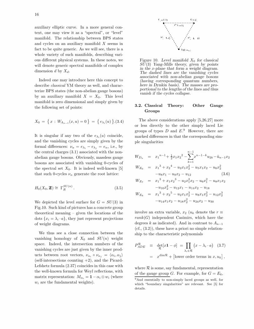
We depicted the level surface for G = SU(3) in

Fig.10. Such kind of pictures has a concrete group

theoretical meaning – given the locations of the

dots xi = λi · a, they just represent projections

of weight diagrams.

We thus see a close connection between the

vanishing homology of X0 and SU(n) weight

space. Indeed, the intersection numbers of the

vanishing cycles are just given by the inner prod-

ucts between root vectors, ναi ναj

= 〈αi, αj〉(self-intersections counting +2), and the Picard-

Lefshetz formula (2.37) coincides in this case with

the well-known formula for Weyl reflections, with

matrix representation: Mαi= 1−αi ⊗wi (where

wi are the fundamental weights).

Figure 10. Level manifold X0 for classicalSU(3) Yang-Mills theory, given by pointsin the x-plane that form a weight diagram.The dashed lines are the vanishing cyclesassociated with non-abelian gauge bosons(having corresponding quantum numbers,here in Dynkin basis). The masses are pro-portional to the lengths of the lines and thusvanish if the cycles collapse.

3.2. Classical Theory: Other Gauge

Groups

The above considerations apply [5,26,27] more

or less directly to the other simply laced Lie

groups of types D and E.9 However, there are

marked differences in that the corresponding sim-

ple singularities

WDn= x1

n−1+ 12x1x2

2 −n−1∑

k=1

xn−1−ku2k−un−1x2

WE6= x1

3 + x24 − u2x1x

22 − u5x1x2 − u6x

22

−u8x1 − u9x2 − u12 (3.6)

WE7= x1

3 + x1x23 − u2x

21x2 − u6x

21 − u8x1x2

−u10x22 − u12x1 − u14x2 − u18

WE8= x1

3 + x25 − u2x1x

32 − u8x1x

22 − u12x

32

−u14x1x2 − u18x22 − u24x2 − u30

involve an extra variable, x2 (uk denote the r ≡rank(G) independent Casimirs, which have the

degrees k as indicated). And in contrast to An−1

(cf., (3.2)), these have a priori no simple relation-

ship to the characteristic polynomials

PRADE ≡ det

R[x1− φ] =

∏

λi∈R

(x− λi · a

)(3.7)

= xdimR +[lower order terms in x, uk

],

where R is some, say fundamental, representation

of the gauge group G. For example, for G = E6,9And essentially to non-simply laced groups as well, for

which “boundary singularities” are relevant. See [5] for

details.

17

WE6(x1, x2) is of degree 12, while P 27

E6(x) is of

order 27 – so these polynomials are really quite

different from each other. The point is that the

equations WADE = 0 and PRADE = 0 have the

same relevant information content (in fact, for ar-

bitrary representations R); the simple singulari-

ties (3.6) are in a sense more efficient in encod-

ing this information, in that the overall scaling

degree is minimized (given by the dual Coxeter

number h), at the expense of introducing another

variable, x2.

In effect, both equations W = 0 and P = 0 can

be taken to define an auxiliary spectral surface

X . However, for D,E gauge groups the surfaces

W (x1, x2) = 0 happen to be no longer zero di-

mensional. 10 For Dn one can “integrate out” the

variable x2 and thereby relate W = 0 to P = 0.

That is, we can simply eliminate x2 via the “equa-

tion of motion” ∂x2WDn

(x1, x2) = 0. Multiplying

WDnby x1 and substituting x1 = x2, we then in-

deed get

x2n −n−1∑

k=1

x2n−2ku2k − 12 u

2n−1 ≡ P 2n

Dn(x, u) = 0.

The relation between W = 0 and P = 0 is how-

ever much more complicated for the exceptional

groups; see [29] for E6.

3.3. Quantum SU(n) Gauge Theory

We now turn to the quantum version of the

N =2 Yang-Mills theories, where the issue is to

construct curvesX1 whose moduli spaces give the

supposed quantum moduli spaces, Mq. We have

seen that the classical theories are characterized

by simple singularities, so we may expect that

the quantum versions should also have something

to do with them. Indeed, for G = SU(n) the

appropriate manifolds were found in [25] and can

be represented by

X1 : y2 =(WAn−1

(x, ui))2 − Λ2n , (3.8)

which corresponds to special genus g = n − 1

hyperelliptic curves. Above, Λ is the dynamically10Actually, as we will see later, the best way to think about

this is to add a third variable x3 and promote W = 0 to

an “ALE space”.

generated quantum scale.

Since y2 factors into WAn−1±Λn, the situation

is in some respect like two copies of the classical

theory, with the top Casimir un shifted by ±Λn.

Specifically, the points eλiof the classical level

surface (3.4) split as follows,

eλi(u) → e±λi

(u,Λ) ≡ eλi(u2, , ..., un−1, un±Λn) ,

and become the 2n branch points of the Riemann

surface (3.8). The curve can accordingly be repre-

sented by the two-sheeted x-plane with cuts run-

ning between pairs e+λiand e−λi

. See Fig.11 for an

example.

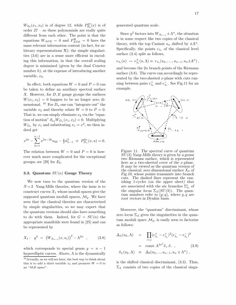
Figure 11. The spectral curve of quantumSU(3) Yang-Mills theory is given by a genustwo Riemann surface, which is representedhere as a two-sheeted cover of the x-plane.It may be viewed as the quantum version ofthe classical, zero dimensional surface X0 ofFig.10, whose points transmute into branchcuts. The dashed lines represent the van-ishing 1-cycles (on the upper sheet) thatare associated with the six branches Σi

± ofthe singular locus ΣΛ(SU(3)). The quan-tum numbers refer to (g; q), where g, q areroot vectors in Dynkin basis.

Moreover, the “quantum” discriminant, whose

zero locus ΣΛ gives the singularities in the quan-

tum moduli space Mq, is easily seen to factorize

as follows:

∆Λ(uk,Λ) =∏

i<j

(e+λi− e+λj

)2(e−λi− e−λj

)2

= const.Λ2n2

δ+ δ− , (3.9)

δ±(uk,Λ) ≡ ∆0(u2, ..., un−1, un ± Λn) ,

is the shifted classical discriminant, (3.3). Thus,

ΣΛ consists of two copies of the classical singu-

18

lar locus Σ0, shifted by ±Λn in the un direction.

Obviously, for Λ → 0, the classical moduli space

is recovered: ΣΛ → Σ0. That is, when the quan-

tum corrections are switched on, a single isolated

branch Σαi

0 of Σ0 (associated with massless gauge

bosons of a particular SU(2) subgroup) splits into

two branches Σi± of ΣΛ (reflecting two massless

dyons related to this SU(2)). For G = SU(3),

this is depicted in Fig.12.

Figure 12. When switching to the exactquantum theory, the classical singular lo-cus splits into two quantum loci that areassociated with massless dyons; this is com-pletely analogous to Fig.2. The distance isgoverned by the quantum scale Λ. Shownare here the six branches Σi

± forG = SU(3).

According to the line of arguments given be-

low equ. (2.35), all what it takes to determine

the dyon spectrum associated with the n(n − 1)

singular branches, is to determine the set of one-

cycles νi± that vanish on the Σi

±, with respect to

some appropriate symplectic basis of α and β cy-

cles. This can be done by tracing the exchange

paths of the branch points e±λiwhen we encir-

cle the components of the discriminant Σi± in the

moduli space (starting from and ending at an ar-

bitrary, but fixed base point).11

11Hypertex capable on-line readers may click here to ob-

tain a Mathematica notebook that shows how this can be

done in practice.

The result can be characterized in a very sim-

ple way: the punctured x-plane (cf., Fig.11) can

be thought of as a “quantum deformation” of the

classical level surface X0 (cf., Fig.10), and thus

inherits its group theoretical properties. We al-

ready mentioned above that the points eλiof X0,

associated with the projected weight vectors λi,

turn into branch cuts, whose length is governed

by the quantum scale, Λ (in fact, one obtains two,

slightly rotated copies of the weight diagram).

Now, a basis of cycles can be chosen such that

the coordinates of the “electric” α-type of cycles

around the cuts are given precisely by the corre-

sponding weight vectors λi. That is, we can as-

sociate charges (g; q) = (0;λi) with the α-cycles.

Moreover, the classical cycles of X0 (related to

the roots αi), turn into pairs of “magnetic” β-

type of cycles. By consistently assigning charge

vectors to all vanishing cycles, we can then imme-

diately read off the electric and magnetic quan-

tum numbers of the massless dyons: they are

given by specific combinations of root vectors.

For G = SU(3), this is indicated in Fig.11.

At this point a feature that is novel for SU(n),

n > 2, becomes evident: there are regions in Mq

where mutually non-local dyons become simulta-

neously massless [18]. Indeed, as can be inferred

from Figs.10,11 for G = SU(3), at u ≡ u2 = 0,

v ≡ u3 = ±Λn, dyons are massless whose van-

ishing cycles have non-zero intersection numbers,

νi νj 6= 0; this phenomenon persists for higher

n as well. In other words, their Dirac-Zwanziger

charge product (2.36) does not vanish, and this

means, as mentioned before, that they are not

local with respect to each other.

Whenever this happens, then by general argu-

ments [30] the theory becomes conformally in-

variant. From (3.8) it is clear that near such an

“Argyres-Douglas” point the curve looks locally

like y2 = WAn−1= xn + ..., and thus effectively

behaves like a genus g = (n − 1)/2 (for n =odd,

g = n/2 − 1 for even n) curve that has a singu-

larity of type An−1. This is the same singular-

ity type that the classical level set X0 (3.4) has

at the conformally invariant point, ul = 0. In-

deed one may view the AD points as arising from

19

“splitting and shifting” the classical An−1 singu-

larities,12 analogously to what saw in Fig.2 for

SU(2). However, whereas the classical theory has

a gauge symmetry at the singularity, the SW the-

ory appears not to have massless gauge bosons at

the AD points [18]. Rather, the SW theory may

have some sort of novel symmetry, but this is not

yet completely settled.

To obtain the effective action (i.e., prepoten-

tial [31,24]), one must first determine the sections

ai(uk), aD,i(uk) ≡ ∂aiF(a), appropriately defined

as period integrals. For theories with more than

one modulus, the existence of a prepotential poses

an integrability condition, which can be solved by

finding a suitable meromorphic one-form λSW .

More specifically, the genus of the hyperelliptic

curve X1 (3.8) is equal to g = n − 1, so that its

2n− 2 periods can naturally be associated with

~π ≡(~aD

~a

). (3.10)

On such a curve there are n− 1 holomorphic dif-

ferentials (abelian differentials of the first kind)

ωn−i = xi−1 dxy , i = 1, . . . , g, out of which one

can construct n − 1 sets of periods∫

γjωi. (Here

γj, j = 1, . . . , 2g, is any basis of H1(X1,ZZ).) All

periods together can be combined in the (g, 2g)-

dimensional period matrix

Πij =

∫

γj

ωi . (3.11)

If we chose a symplectic homology basis, i.e.

αi = γi, βi = γg+i, i = 1, . . . , g, with intersection

pairing13 (αi βi) = δij , (αi αj) = (βi βj) = 0,

and if we write Π = (A,B), then τ ≡ A−1B is

the metric on the quantum moduli space. By

Riemann’s second relation, Im(τ) ≡ 8π2/g2eff is

manifestly positive, which is important for unitar-

ity of the effective N = 2 supersymmetric gauge

theory.12This generalized to a whole series of d = 4, N = 2 su-

perconformal theories, classified by the ADE Lie algebras

[30].13We use the convention that a crossing between the cycles

α, β counts positively to the intersection (αβ), if looking

in the direction of the arrow of α the arrow of β points to

the right.

The precise relation between the periods and

the components of the section ~π is given by:

Aij =

∫

αj

ωi =∂

∂ui+1aj

Bij =

∫

βj

ωi =∂

∂ui+1aDj

(3.12)

(where i, j = 1, . . . , n − 1). From the explicit

expression (3.8) for the family of hyperelliptic

curves, one immediately verifies that the integra-

bility conditions ∂i+1Ajk = ∂j+1Aik, ∂i+1Bjk =

∂j+1Bik are satisfied. It also follows that τij ≡∂ai

∂ajF(a). This reflects the special geometry of

the quantum moduli space, and implies that the

components of ~π can directly be expressed as in-

tegrals

aDi=

∫

βi

λSW , ai =

∫

αi

λSW , (3.13)

over a suitably chosen meromorphic differential.

One may take, for example [32,33]:

λSW =dx

4√

2πlog[WAn−1

+√W 2

An−1−Λ2n

WAn−1−√W 2

An−1−Λ2n

]

=1

2√

2π

( ∂∂xWAn−1

(x, ui))xdx

y+∂[∗]. (3.14)

Explicit expressions for the prepotentials [21,

31,24] can be obtained by first solving Picard-

Fuchs equations, and consequently matching the

solutions with the asymptotic expansions of the

period integrals (in analogy to what we discussed

in section 2.5; recently, a more efficient method

has been developed in ref. [34].) In fact, for a

given group one can write down a whole variety of

effective actions that are valid in appropriate co-

ordinate patches in the moduli space; this is sim-

ilar to what was shown in Fig.3 for G = SU(2).

Specifically, in the semi-classical coordinate

patch, where by definition the classical central

charges are large, eαi≡ αi ·a≫ Λ, the prepoten-

20

tial has the form:14

F(ai) = Fclass + F1−loop + Fnon−pert , (3.15)

where

Fclass =1

2τ0 (at · C · a)

F1−loop =i

4π

∑

positive

roots α

eα2 log [eα

2/Λ2] (3.16)

Fnon−pert = − i

2π

(∑

positive

roots α

eα2) ∞∑

ℓ=1

F2hℓ(eα−1)Λ2hℓ.

Here F2hℓ(eα−1) are Weyl invariant Laurent poly-

nomials in the eα of degree −2hℓ. For exam-

ple, for G = SU(3), F6 = 14

∏α eα

−2; see refs.

[22,34]. for some further explicit expressions for

F2hℓ. The one-loop term, F1−loop, here obtained

from solving a differential equation, indeed coin-

cides exactly with what one obtains by a standard

perturbative quantum field theory computation !

3.4. Fibrations of Weight Diagrams

There is an alternative representation of the

SW curves X1, which is not manifestly hyperge-

ometric and thus perhaps slightly less convenient

to deal with, but which can easily be generalized

to arbitrary gauge groups. As we will see, it is also

precisely this geometrically more natural form of

the curves that arises in string theory [6].

Inspired by the role of spectral curves in inte-

grable systems [7,27,35], one is lead to consider

SW curves (3.8) of the form [7,27]:

X1 : z +Λn

z+ 2Pn

An−1(x, uk) = 0 , (3.17)

where the characteristic polynomial (3.8) for

SU(n) obeys “by accident” : PnAn−1

≡ WAn−1.

These curves are related to the hyperelliptic

curves (3.8) by a simple reparametrization, z →y−P , and thus are completely equivalent to them.

14This form is valid for all ADE groups; C denotes the

Cartan matrix, τ0 the bare coupling and h the dual Cox-

eter number (h ≡ n for SU(n)).

Figure 13. The Seiberg-Witten curve can beunderstood as fibration of a weight diagram(the classical surface X0 of Fig.10 over IP1.Pairs of singular points in the base are asso-ciated with vanishing 0-cycles in the fiber,i.e., to root vectors ai−aj . In string theory,the local fibers will be replaced by appropri-ate ALE spaces with corresponding vanish-ing two-cycles.

Moreover, note also that the classical limit Λ → 0

gives X1 : z + P (x) = 0, which is an (equiv-

alent) alternative to the classical level surfaces,

X0: P (x) = 0.

A curve of the form (3.17) can be thought as

fibration of the classical level setX0 (3.4) over IP1,

coordinatized by z and whose size is measured by

1/Λ. There are (n − 1) pairs of branch points

in the z-plane, z±i , which are associated with the

basic degenerations of X0, ie., with the simple

roots αi. There are two additional branch points

z0, z∞, and cuts run between, say z−i and z0, and

between z+αi

and z∞. See Fig.13 for G = SU(3),

where X1 : z + Λ3/z + 2(x3 − ux− v) = 0 and

z±1 = 2u32 + 3

√3v ±

√(2u

32 + 3

√3v)2

− Λ6

z±2 = −2u32 + 3

√3v ±

√(2u

32 − 3

√3v)2

− Λ6 .

The curve may also be viewed as a foliation, or n-

sheeted covering of the z-plane, the sheets being

associated to the points of X0, ie., to the weights

λi, see Fig.14.15

The meromorphic differential takes the follow-

15One may draw the cuts also in different ways; we have

chosen them here such that the massless monopoles are

related to vanishing β-type cycles.

21

z

Figure 14. The genus two curve resultingfrom the fibration shown in Fig.13 can beviewed as a foliation with three leaves thatare glued together over the cuts. The sheetsare one-to-one to the weights of the funda-mental representation of SU(3).

ing particularly simple form,

λSW =1

2√

2πx(z, u)

dz

z. (3.18)

which, via partial integration, is equivalent to

(3.14). Note that there are actually n versions

of λSW , since x(z) ∼ z1/n, each associated to one

of the sheets of the foliation.

Having represented the SU(n) curves in the

form (3.17), the generalization to other simply

laced groups is now easy to state [27]: one just

takes the characteristic polynomial PRADE (3.8)

(for an arbitrary representation R), and shifts the

top Casimir uh by z + Λh

z , i.e.,

X1 : PRADE(x, uk, uh + z +

Λh

z) = 0 , (3.19)

where h is the dual Coxeter number. As explained

in [27], the choice of the representation is irrele-

vant. That is, there is for each gauge group an

infinity of possible curves, with arbitrarily high

genera; however, one can restrict attention to a

particular subset of r ≡ rank(G) α- and r dual

β-periods, which carry all the relevant informa-

tion.

On can in fact write down curves for the non-

simply laced groups as well. These are obtained

by fibering ADE level surfaces PRADE = 0 in a

“non-split” fashion, i.e., in a way that encircling

the singular points in the z-plane gives rise not

only to Weyl transformations acting on the fiber

X0, but also to outer automorphisms. This is

similar to the considerations of [36], and gives

an orbifold prescription leading to a “folding” of

the ADE Dynkin diagram into the corresponding

non-simply laced one; it also appropriately mod-

ifies the curves (3.19)[27].

4. SW Geometry from String Duality

4.1. General Picture

So far, the auxiliary “spectral curves”

(3.8),(3.17),(3.19) have been introduced in a

somewhat ad hoc fashion, originally just in order

to deal with the monodromy problem in a system-

atic way. One may in fact approach the SW the-

ory without directly referring to a Riemann sur-

face, for example along the lines of [37], but this

gets pretty quickly out of hand for larger gauge

groups. Thus the question comes up whether the

SW curves have a more concrete physical signif-

icance – it would be rather absurd if all the ge-

ometrical richness of Riemann surfaces would be

nothing more than a technical convenience, and

would not have any deeper meaning.

This attitude is supported by growing recent

experience that whenever we meet a geometri-

cal object like a spectral manifold, it represents a

concrete physical object in some appropriate dual

formulation of the theory. For example, the clas-

sical level set X0 (3.4), consisting of a discrete

set of points, has been associated with the loca-

tions of D-branes in a dual formulation of gauge

symmetry enhancement [38] – the dashed lines in

Fig.10 then are nothing but open strings linking

D-branes.

Indeed it turns out [6] that, in this sense, the

natural home of SW geometry is string theory,

but of a rather peculiar, “non-critical” kind [39,

40].

For ease of discussion it is most convenient to

start with ordinary, “critical” superstrings that

naturally live in ten dimensions. Remember that

for these theories, complex manifolds play an

ubiquitous role as compactification manifolds –

22

and this already hints at our aim to ultimately

view the SW curves as some kind of compactifi-

cation manifolds as well.

K3 surface CY 3-fold

SW curveclass spectr set

local singularity

fibration

fibration

local singularity

Figure 15. Complex manifolds that are rel-evant in heterotic-type II duality. The ver-tical direction is a local scaling limit thatincludes switching off α′. The horizontalstep corresponds to switching on space-timequantum corrections.

More specifically, what we have in mind is a

structure roughly as depicted in Fig.15. That

is, starting from the spectral set X0, which de-

scribes classical Yang-Mills theory, one can go to

the quantum version via fibering X0 over IP1 with

size 1/Λ – this was described in section 3.4. How-

ever, one may also go vertically and view X0 (and

thus classical, N = 4 Yang-Mills theory itself) as

arising from a particular multiple scaling limit of

a K3 compactification (which includes the limit

α′ → 0). This K3 surface X2 may then itself be

taken as a fiber over IP1, to yield a Calabi-Yau

threefold X3. One may thus expect to close the

circle in Fig.15 by performing a suitable limit of

X3, in order to get back to the SW curve. How

this exactly works will be explained in the next

couple of sections.

4.2. ALE Spaces and Heterotic-Type II

String Duality in Six Dimensions

Fig.15 may look suggestive, but so far we did

not specify the precise physical context to which

it is supposed to apply. The correct framework is

the duality [2,41,42] between the heterotic string

and the type II string that appears when the

strings are compactified on suitable manifolds.

See [43] for a detailed review on this subject.

Let us first review the original Hull-Townsend

hypothesis, which states the non-perturbative

equivalence of the heterotic string (compactified

on T4) with the type IIA string (compactified on

K3). As is well-known, gauge symmetry arises

in the six-dimensional heterotic string from the

Narain lattice, Γ20,4. More precisely, ADE type

of gauge symmetries arise if the background mod-

uli are such that the Narain lattice becomes ADE

symmetric, i.e., if there are lattice vectors with

(length)2 = 2. These are just the root vectors

associated with the gauge group, and give rise to

space-time gauge fields via the Frenkel-Kac mech-

anism (see eg., [44]).

On the type IIA string side, gauge symme-

tries arise from ADE type of singularities of K3

[2,45,46,38,47]. More specifically, if the K3 mod-

uli are tuned appropriately, K3 can locally (near

the singularity and in some suitable coordinate

patch) be written as:

WK3 = ǫ[WALE

ADE

]+ O(ǫ2) = 0 , (4.1)

where, in physical terms, ǫ∼ (α′)σ → 0 for some

power σ. Moreover, SADE : WALEADE(xi) = 0 is

the Asymptotically Local Euclidean space [48]

with ADE singularity at the origin; it is a non-

compact space obtained by excising a small neigh-

borhood around the singularity on K3. This kind

of spaces is essentially given by the ADE simple

singularities (3.2), (3.6), up to “morsification” by

extra quadratic pieces:

WALEAn−1

= WAn−1(x1, uk) + x2

2 + x32

= x1n + x2

2 + x32 + . . . (4.2)

WALED,E = WD,E(x1, x2, uk) + x3

2 .

In fact, the ADE singularities can be character-

ized in a most uniform and natural way if they

are written, exactly as above, as ALE space sin-

gularities in terms of three variables. By defini-

tion, SADE = C3/[WADE = 0], but one may also

write SADE = C2/Γ, where Γ = Cn,Dn, T ,O, I ⊂SL(2,C) are the discrete isometry groups of the

sphere that are canonically associated with the

ADE groups [5,28].

The variables uk provide a minimal resolution

of these singularities, obtained by iterated blow

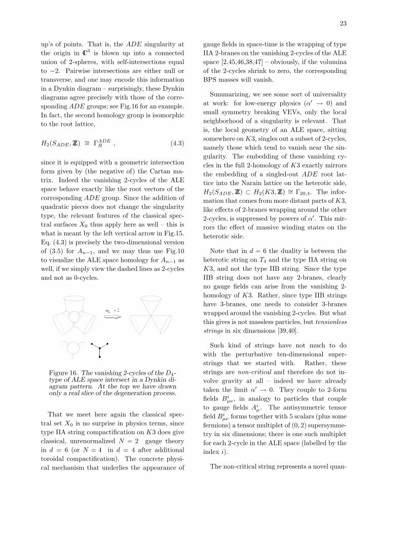
23

up’s of points. That is, the ADE singularity at

the origin in C3 is blown up into a connected

union of 2-spheres, with self-intersections equal

to −2. Pairwise intersections are either null or

transverse, and one may encode this information

in a Dynkin diagram – surprisingly, these Dynkin

diagrams agree precisely with those of the corre-

sponding ADE groups; see Fig.16 for an example.

In fact, the second homology group is isomorphic

to the root lattice,

H2(SADE ,ZZ) ∼= ΓADER , (4.3)

since it is equipped with a geometric intersection

form given by (the negative of) the Cartan ma-

trix. Indeed the vanishing 2-cycles of the ALE

space behave exactly like the root vectors of the

corresponding ADE group. Since the addition of

quadratic pieces does not change the singularity

type, the relevant features of the classical spec-

tral surfaces X0 thus apply here as well – this is

what is meant by the left vertical arrow in Fig.15.

Eq. (4.3) is precisely the two-dimensional version

of (3.5) for An−1, and we may thus use Fig.10

to visualize the ALE space homology for An−1 as

well, if we simply view the dashed lines as 2-cycles

and not as 0-cycles.

Figure 16. The vanishing 2-cycles of theD4-type of ALE space intersect in a Dynkin di-agram pattern. At the top we have drawnonly a real slice of the degeneration process.

That we meet here again the classical spec-

tral set X0 is no surprise in physics terms, since

type IIA string compactification on K3 does give

classical, unrenormalized N = 2 gauge theory

in d = 6 (or N = 4 in d = 4 after additional

toroidal compactification). The concrete physi-

cal mechanism that underlies the appearance of

gauge fields in space-time is the wrapping of type

IIA 2-branes on the vanishing 2-cycles of the ALE

space [2,45,46,38,47] – obviously, if the volumina

of the 2-cycles shrink to zero, the corresponding

BPS masses will vanish.

Summarizing, we see some sort of universality

at work: for low-energy physics (α′ → 0) and

small symmetry breaking VEVs, only the local

neighborhood of a singularity is relevant. That

is, the local geometry of an ALE space, sitting

somewhere onK3, singles out a subset of 2-cycles,

namely those which tend to vanish near the sin-

gularity. The embedding of these vanishing cy-

cles in the full 2-homology of K3 exactly mirrors

the embedding of a singled-out ADE root lat-

tice into the Narain lattice on the heterotic side,

H2(SADE ,ZZ) ⊂ H2(K3,ZZ) ∼= Γ20,4. The infor-

mation that comes from more distant parts ofK3,

like effects of 2-branes wrapping around the other

2-cycles, is suppressed by powers of α′. This mir-

rors the effect of massive winding states on the

heterotic side.

Note that in d = 6 the duality is between the

heterotic string on T4 and the type IIA string on

K3, and not the type IIB string. Since the type

IIB string does not have any 2-branes, clearly

no gauge fields can arise from the vanishing 2-

homology of K3. Rather, since type IIB strings

have 3-branes, one needs to consider 3-branes

wrapped around the vanishing 2-cycles. But what

this gives is not massless particles, but tensionless

strings in six dimensions [39,40].

Such kind of strings have not much to do

with the perturbative ten-dimensional super-

strings that we started with. Rather, these

strings are non-critical and therefore do not in-

volve gravity at all – indeed we have already

taken the limit α′ → 0. They couple to 2-form

fields Biµν , in analogy to particles that couple

to gauge fields Aiµ. The antisymmetric tensor

field Biµν forms together with 5 scalars (plus some

fermions) a tensor multiplet of (0, 2) supersymme-

try in six dimensions; there is one such multiplet

for each 2-cycle in the ALE space (labelled by the

index i).

The non-critical string represents a novel quan-

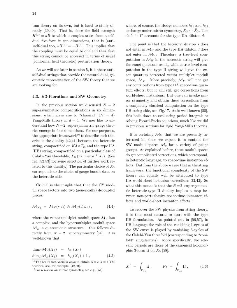
24

tum theory on its own, but is hard to study di-

rectly [39,40]. That is, since the field strength

H(3) = dB to which it couples arises from a self-

dual five-form in ten dimensions, that is (anti-

)self-dual too, ∗H(3) = −H(3). This implies that

the coupling must be equal to one and thus that

this string cannot be accessed in terms of usual

(conformal field theoretic) perturbation theory.

As we will see later in section 5, it is these anti-

self-dual strings that provide the natural dual, ge-

ometric representation of the SW theory that we

are looking for.

4.3. K3-Fibrations and SW Geometry

In the previous section we discussed N = 2

supersymmetric compactifications in six dimen-

sions, which gives rise to “classical” (N = 4)

Yang-Mills theory in d = 4. We now like to un-

derstand how N=2 supersymmetric gauge theo-

ries emerge in four dimensions. For our purposes,

the appropriate framework16 to describe such the-

ories is the duality [42,41] between the heterotic

string, compactified on K3×T2, and the type IIA

(IIB) string, compactified on a particular class of

Calabi-Yau threefolds, X3 (its mirror17 X3). (See

ref. [52,53] for some selection of further work re-

lated to this duality.) The particular choice of X3

corresponds to the choice of gauge bundle data on

the heterotic side.

Crucial is the insight that that the CY mod-

uli space factors into two (generically) decoupled

pieces:

MX3= MV (s, ti) ⊗ MH(d, hk) , (4.4)

where the vector multiplet moduli space MV has

a complex, and the hypermultiplet moduli space

MH a quaternionic structure – this follows di-

rectly from N = 2 supersymmetry [54]. It is

well-known that

dimCMV (X3) = h11(X3)

dimCMH(X3) = h21(X3) + 1 , (4.5)16The are in fact various ways to obtain N =2 d = 4 YM

theories, see, for example, [49,50].17For a review on mirror symmetry, see e.g., [51].

where, of course, the Hodge numbers h11 and h22

exchange under mirror symmetry, X3 ↔ X3. The

shift “+1” accounts for the type IIA dilaton d.

The point is that the heterotic dilaton s does

not enter in MH and the type IIA dilaton d does

not enter in MV . Therefore, a tree-level com-

putation in MH in the heterotic string will give

the exact quantum result, while a tree-level com-

putation in the type II string will give the ex-

act quantum corrected vector multiplet moduli

space, MV . More precisely, MV will not get

any contributions from type IIA space-time quan-

tum effects, but it will still get corrections from

world-sheet instantons. But one can invoke mir-

ror symmetry and obtain these corrections from

a completely classical computation on the type

IIB string side, see Fig.17. As is well-known [55],

this boils down to evaluating period integrals or

solving Picard-Fuchs equations, much like we did

in previous sections for rigid Yang-Mills theories.

It is certainly MV that we are presently in-

terested in, since we expect it to contain the

SW moduli spaces Mq for a variety of gauge

groups. As explained before, these moduli spaces

do get complicated corrections, which correspond,

in heterotic language, to space-time instanton ef-

fects. But from the above we see that in the string

framework, the functional complexity of the SW

theory can equally well be attributed to type

IIA world-sheet instanton corrections [32,42]. So

what this means is that the N=2 supersymmet-

ric heterotic-type II duality implies a map be-

tween non-perturbative space-time instanton ef-

fects and world-sheet instanton effects !

To recover the SW physics from string theory,

it is thus most natural to start with the type

IIB formulation. As pointed out in [56,57], in

IIB language the role of the vanishing 1-cycles of

the SW curve is played by vanishing 3-cycles of

the Calabi-Yau threefold (corresponding to “coni-

fold” singularities). More specifically, the rele-

vant periods are those of the canonical holomor-

phic 3-form Ω on X3 [58]:

XI =

∫

ΓαI

Ω , FJ =

∫

ΓβJ

Ω , (4.6)

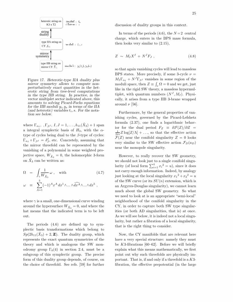
25

heterotic string onK3 x T2

type IIA string on

CY

dualitystring

symmetrymirror

type IIB string onmirror CY

Figure 17. Heterotic-type IIA duality plusmirror symmetry allows to compute non-perturbatively exact quantities in the het-erotic string from tree-level computationsin the type IIB string. In practice, in thevector multiplet sector indicated above, thisamounts to solving Picard-Fuchs equationsfor the IIB moduli yi, ys in terms of the IIA(and heterotic) variables ti, s. For the nota-tion see below.

where ΓαI, ,ΓβJ , I, J = 1, . . . , h11(X3) + 1 span

a integral symplectic basis of H3, with the α-

type of cycles being dual to the β-type of cycles:

ΓαI ΓβJ = δI

J , etc. Concretely, assuming that

the mirror threefold can be represented by the

vanishing of a polynomial in some weighted pro-

jective space, WX3= 0, the holomorphic 3-form

on X3 can be written as:

Ω =

∫

γ

1

WX3

ω , with (4.7)

ω ≡5∑

A=1

(−1)AxA dx1∧... ∧dxA∧...∧dx5 ,

where γ is a small, one-dimensional curve winding

around the hypersurface WX3= 0, and where the

hat means that the indicated term is to be left

out.

The periods (4.6) are defined up to sym-

plectic basis transformations which belong to

Sp(2h11(X3) + 2,ZZ). The duality group, which

represents the exact quantum symmetries of the

theory and which is analogous the SW mon-

odromy group Γ0(4) in section 2.4, must be a

subgroup of this symplectic group. The precise

form of this duality group depends, of course, on

the choice of threefold. See refs. [59] for further

discussion of duality groups in this context.

In terms of the periods (4.6), the N=2 central

charge, which enters in the BPS mass formula,

then looks very similar to (2.15),

Z ∼ MIXI + NJFJ , (4.8)

so that again vanishing cycles will lead to massless

BPS states. More precisely, if some 3-cycle ν =

MIΓαI+ NJΓβJ vanishes in some region of the

moduli space, then Z ≡∫

νΩ = 0 and we get, just

like in the rigid SW theory, a massless hypermul-

tiplet, with quantum numbers (NJ ,MI). Physi-

cally, it arises from a type IIB 3-brane wrapped

around ν [56].

Furthermore, by the general properties of van-

ishing cycles, governed by the Picard-Lefshetz

formula (2.37), one finds a logarithmic behav-

ior for the dual period FZ ≡ ∂F(Z)/∂Z =1

2πiZ log[Z/Λ] + . . ., so that the effective action

F(Z) near the conifold singularity Z = 0 looks

very similar to the SW effective action FD(aD)

near the monopole singularity.

However, to really recover the SW geometry,

we should not look just to a single conifold singu-

larity (of local form∑4

i=1 xi2 = u), since it does

not carry enough information. Indeed, by analogy

just looking at the local singularity x12 +x2

2 = u

of the SW curve (or its SU(n) extension, which is

an Argyres-Douglas singularity), we cannot learn

much about the global SW geometry. So what

we need to look at is an appropriate “semi-local”

neighborhood of the conifold singularity in the

CY, in order to capture both SW type singular-

ities (or both AD singularities, that is) at once.

As we will see below, it is indeed not a local singu-

larity, but rather a fibration of a local singularity,

that is the right thing to consider.

Now, the CY manifolds that are relevant here

have a very special structure: namely they must

be K3-fibrations [60–62]. Before we will briefly

explain what this means mathematically, we first

point out why such threefolds are physically im-

portant. That is, if and only if a threefold is aK3-

fibration, the effective prepotential (in the large

26

radius limit) has this particular asymptotic form:

F(s, t) =1

2sQijt

itj +1

6Cijkt

itjtk + . . . . (4.9)

Here, Q and C directly reflect the classical inter-

section properties of 2-cycles, and s, ti are Kahler

moduli of the CY, where s is singled out in that

it couples only linearly. This means that s can

naturally be identified (to leading order) with the

semi-classical dilaton of the heterotic string, since

the dilaton couples exactly in this way.

The K3 fibration structure turns out to be cru-

cial for our purposes. To see this, let us assume,

for simplicity, that the (mirror) threefold X3 can

be represented by some polynomial

X3 : WX3(x1, x2, x3, x4, x5; yi, ys) = 0 (4.10)

in weighted projective space W IP2d1,1,2k1,2k2,2k3

,

with overall degree 2d ≡ 2(1 + k1 + k2 + k3).

Above, yi denote the moduli, and, in particular,

ys denotes the special distinguished modulus that

is related to the heterotic dilaton, ys ∼ e−s. A

list of this kind ofK3 fibered threefolds was given

in [60]. (For more general classes of fibrations, see

[63]. Considerations similar to those below apply

to these cases as well.)

The statement that X3 is a K3 fibration of this

particular type means that it can be written as

WX3(xj ; yi, ys) =

1

2d

(x1

2d+x22d+

2√ys

(x1x2)d)

+ W (x1x2

ys1/d

, xk; yi) . (4.11)

Upon the variable substitution

x1 =√x0 ζ

1/2d

x2 =√x0 ζ

−1/2dys1/2d (4.12)

this gives

WX3(xj ; ζ, yi) =

1

2d

(ζ+

ys

ζ+2)xd

0+W (x0, xk; yi).

That is, if we now alternatively view ζ as

a modulus, and not as a coordinate, then

WX3(ζ, x2, x3, x4, x5; yi, ys)≡WK3(x2, x3, x4, x5;

ζ + ys

ζ , yi) = 0 describes a K3 – this is precisely

what is meant by fibration (of course, if we con-

tinue to view ζ as a coordinate, then this equation

still describes the Calabi-Yau threefold). More

precisely, ζ is the coordinate of the base IP1, and

ys → 0 corresponds to the large base limit – ob-

viously, the fibration looks in this limit locally

trivial, and one expects then the theory to be

dominated by the “classical” physics of the K3

(cf., the top horizontal step in Fig.15). This is

the “adiabatic limit” [61], in which the K3 fibers

vary only slowly over the base and where one can

apply the original Hull-Townsend duality fiber-

wise.

The left-over piece W is precisely such that1dx

d0 + W (x0, xk; yi) = 0 describes a K3 in canon-

ical parametrization in W IPd1,k1,k2,k3

. Now as-

suming that the K3 is singular of type ADE in

some region of the moduli space, we can expand

it around the critical point and thereby replace it

locally by the ALE normal form (4.2) of the sin-

gularity, 1dx

d0 + W ∼ ǫWALE

ADE(xi, uk). Going to

the patch x0 = 1 and rescaling18 ys = ǫ2Λ2h and

ζ = ǫ z, we then obtain the following fibration of

the ALE space:

WX3(xj , z;uk) = (4.13)

ǫ(z +

Λ2h

z+ 2WALE

ADE(xj , uk))

+ O(ǫ2) = 0.

This is not totally surprising: since the CY was a

K3 fibration, considering a region in moduli space

where the K3 can be approximated by an ALE

space simply produces locally a corresponding fi-

bration of the ALE space.

Now, focusing on G = SU(n) ∼ An−1 and

remembering the definition of the ALE space

(4.2), we see that (4.13) is exactly the same as

the fibered form of the SW curve (3.17), apart

from the extra quadratic pieces in x2, x3 ! Since

quadratic pieces do not change the local singu-

larity type, this means that the local geometry

of the threefold in the SW regime of the mod-

uli space is indeed equivalent to the one of the

Seiberg-Witten curve. However, just because of

18 This fixes ǫ = (α′)h/2.

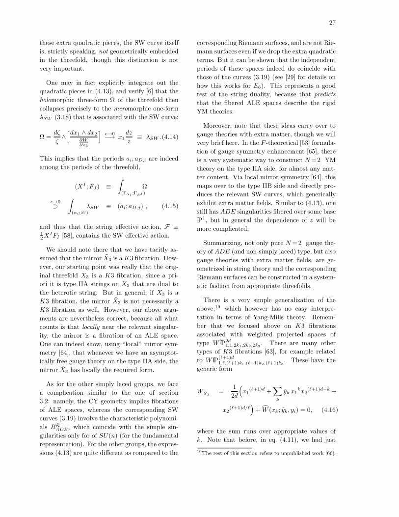
27

these extra quadratic pieces, the SW curve itself

is, strictly speaking, not geometrically embedded

in the threefold, though this distinction is not

very important.

One may in fact explicitly integrate out the

quadratic pieces in (4.13), and verify [6] that the

holomorphic three-form Ω of the threefold then

collapses precisely to the meromorphic one-form

λSW (3.18) that is associated with the SW curve:

Ω =dζ

ζ∧[dx1 ∧ dx2

∂W∂x3

]ǫ→0−→ x1

dz

z≡ λSW .(4.14)

This implies that the periods ai, aD,i are indeed

among the periods of the threefold,

(XI ;FJ ) ≡∫

(ΓαI;Γ

βJ )

Ω

ǫ→0⊃∫

(αi;βj)

λSW ≡ (ai; aD,j) , (4.15)

and thus that the string effective action, F ≡12X

IFI [58], contains the SW effective action.

We should note there that we have tacitly as-

sumed that the mirror X3 is a K3 fibration. How-

ever, our starting point was really that the orig-

inal threefold X3 is a K3 fibration, since a pri-

ori it is type IIA strings on X3 that are dual to

the heterotic string. But in general, if X3 is a

K3 fibration, the mirror X3 is not necessarily a

K3 fibration as well. However, our above argu-

ments are nevertheless correct, because all what

counts is that locally near the relevant singular-

ity, the mirror is a fibration of an ALE space.

One can indeed show, using “local” mirror sym-

metry [64], that whenever we have an asymptot-

ically free gauge theory on the type IIA side, the

mirror X3 has locally the required form.

As for the other simply laced groups, we face

a complication similar to the one of section

3.2: namely, the CY geometry implies fibrations

of ALE spaces, whereas the corresponding SW

curves (3.19) involve the characteristic polynomi-

als RRADE , which coincide with the simple sin-

gularities only for of SU(n) (for the fundamental

representation). For the other groups, the expres-

sions (4.13) are quite different as compared to the

corresponding Riemann surfaces, and are not Rie-

mann surfaces even if we drop the extra quadratic

terms. But it can be shown that the independent

periods of these spaces indeed do coincide with

those of the curves (3.19) (see [29] for details on

how this works for E6). This represents a good

test of the string duality, because that predicts

that the fibered ALE spaces describe the rigid

YM theories.

Moreover, note that these ideas carry over to

gauge theories with extra matter, though we will

very brief here. In the F -theoretical [53] formula-

tion of gauge symmetry enhancement [65], there

is a very systematic way to construct N=2 YM

theory on the type IIA side, for almost any mat-

ter content. Via local mirror symmetry [64], this

maps over to the type IIB side and directly pro-

duces the relevant SW curves, which generically

exhibit extra matter fields. Similar to (4.13), one

still has ADE singularities fibered over some base

IP1, but in general the dependence of z will be

more complicated.

Summarizing, not only pure N =2 gauge the-

ory of ADE (and non-simply laced) type, but also

gauge theories with extra matter fields, are ge-

ometrized in string theory and the corresponding

Riemann surfaces can be constructed in a system-

atic fashion from appropriate threefolds.

There is a very simple generalization of the

above,19 which however has no easy interpre-

tation in terms of Yang-Mills theory. Remem-

ber that we focused above on K3 fibrations

associated with weighted projected spaces of

type W IP2d1,1,2k1,2k2,2k3

. There are many other

types of K3 fibrations [63], for example related

to W IP(ℓ+1)d1,ℓ,(ℓ+1)k1,(ℓ+1)k2,(ℓ+1)k3

. These have the

generic form

WX3=

1

2d

(x1

(ℓ+1)d +∑

k

yk x1kx2

(ℓ+1)d−k +

x2(ℓ+1)d/ℓ

)+ W (xk; yk, yi) = 0, (4.16)

where the sum runs over appropriate values of

k. Note that before, in eq. (4.11), we had just

19The rest of this section refers to unpublished work [66].

28

one variable ys in the bracket. The difference is

that we have now ℓ moduli of this sort, yk. Still,

one of the yk is distinguished by the linear cou-

pling property and thus is related to the heterotic

dilaton; we will continue to denote it by ys ∼ e−s.

Also note that before, when we tuned ys → 1, the

term in the bracket became a perfect square, and

hence the threefold singular (of type A1). This

singularity leads in fact to an IR free SU(2) gauge

symmetry that is non-perturbative from the het-

erotic point of view (since ys = 1 corresponds to

strong coupling).

For the K3 fibrations above, we have now ℓ

such parameters, and tuning them appropriately,

there arises an analogous SU(ℓ+ 1) “strong cou-

pling” gauge symmetry [67]. But this is not the

gauge symmetry that we are interested in here,

we are rather still interested in the perturbative

gauge symmetries that come from the K3 singu-

larities. By taking now a singular limit similar to

before, we arrive at the following modified fibra-

tion of the ALE spaces:

WX3(xj , z;uk) ∼ (4.17)

ǫ(zℓ +

ℓ−1∑

m=1

Λ(m) zm+Λ2h

z+2WALE

ADE(xj , uk))

= 0.

This kind of fibrations has obviously a more com-

plicated structure in the base IP1, and indeed we

have now a whole series of extra moduli, Λ(m),

that move the new singular points on the base

around. If we send the extra Λ’s to infinity, we

obviously recover the SW theories as explained

before.

The interesting point is here that the physics

associated to the extra parameters has nothing

to do with the K3 fibers, and thus is intrinsi-

cally non-perturbative from the heterotic point

of view. So what we have here is a marriage of

the SW physics with physics inherited from the

strong-coupling singularity. It results in SW type

of curves that do not simply describe ordinary

Yang-Mills physics. More concretely, in the clas-

sical limit, Λ → 0, the discriminant of (4.17) looks

∆(uk,Λ(m),Λ = 0) =

(∆0(uk)

)2∆(uk,Λ

(m))

∆(uk,Λ(m) = 0) ≡

(∆0(uk)

)ℓ−1, (4.18)

where ∆0 is the classical discriminant (3.3) asso-

ciated with the corresponding ADE gauge group.

The discriminant ∆(Λ = 0) describes a classical

gauge symmetry G = GADE × U(1)ℓ, with extra

matter fields charged under the various group fac-

tors; in general this theory is non-asymptotically

free.

However, for ℓ > 1 the dependence of ∆ on the

Λ(m) is such that it does not describe any classi-

cal gauge theory (an exception is for G = SU(2)

with ℓ = 2, where the theory is identical to the

SU(2) gauge theory with Nf = 1, with Λ(1) play-

ing the role of the bare mass parameter). In other

words, even though we can identify gauge symme-

tries and matter representations, the dependence

of the theory on the extra parameters is in general

not like the dependence on any mass parameters,

or VEV’s (because ∆ 6= ∏weights λ(a · λ+m)).

Rather, the moduli Λ(m) are novel, dilaton-like

parameters that reflect non-perturbative physics

of the heterotic string. Their effects persist even

for weak coupling, Λ → 0, and are thus like “small

instanton” effects [68].

The lesson we draw from this is that “rigid”

limits in string theory will in general not only re-

produce known field theories like Yang-Mills the-

ories and their curves, but also new kinds of SW

like theories that do not have the interpretation in

terms of conventional physics. Indeed, since the

variety of possible CY singularities is quite large,

one may expect to find a whole zoo of supersym-

metric effective theories, and there is no reason

why such theories should always be interpretable

in terms of conventional field theories like gauge

theories.

5. Anti-Self-Dual Strings on Riemann Sur-

faces

5.1. Geometry of Wrapped 3-Branes

In the previous section we have mentioned that

the role of the SW monopole singularity is played

in the CY threefold by a conifold singularity [56].

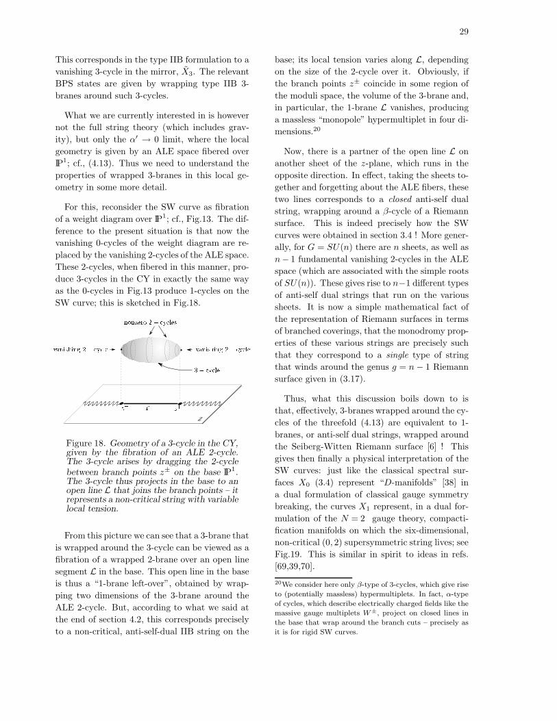
29

This corresponds in the type IIB formulation to a

vanishing 3-cycle in the mirror, X3. The relevant

BPS states are given by wrapping type IIB 3-

branes around such 3-cycles.

What we are currently interested in is however

not the full string theory (which includes grav-

ity), but only the α′ → 0 limit, where the local

geometry is given by an ALE space fibered over

IP1; cf., (4.13). Thus we need to understand the

properties of wrapped 3-branes in this local ge-

ometry in some more detail.

For this, reconsider the SW curve as fibration

of a weight diagram over IP1; cf., Fig.13. The dif-

ference to the present situation is that now the

vanishing 0-cycles of the weight diagram are re-

placed by the vanishing 2-cycles of the ALE space.

These 2-cycles, when fibered in this manner, pro-

duce 3-cycles in the CY in exactly the same way

as the 0-cycles in Fig.13 produce 1-cycles on the

SW curve; this is sketched in Fig.18.

z

Figure 18. Geometry of a 3-cycle in the CY,given by the fibration of an ALE 2-cycle.The 3-cycle arises by dragging the 2-cyclebetween branch points z± on the base IP1.The 3-cycle thus projects in the base to anopen line L that joins the branch points – itrepresents a non-critical string with variablelocal tension.

From this picture we can see that a 3-brane that

is wrapped around the 3-cycle can be viewed as a

fibration of a wrapped 2-brane over an open line

segment L in the base. This open line in the base

is thus a “1-brane left-over”, obtained by wrap-

ping two dimensions of the 3-brane around the

ALE 2-cycle. But, according to what we said at

the end of section 4.2, this corresponds precisely

to a non-critical, anti-self-dual IIB string on the

base; its local tension varies along L, depending

on the size of the 2-cycle over it. Obviously, if

the branch points z± coincide in some region of

the moduli space, the volume of the 3-brane and,

in particular, the 1-brane L vanishes, producing

a massless “monopole” hypermultiplet in four di-

mensions.20

Now, there is a partner of the open line L on

another sheet of the z-plane, which runs in the

opposite direction. In effect, taking the sheets to-

gether and forgetting about the ALE fibers, these

two lines corresponds to a closed anti-self dual

string, wrapping around a β-cycle of a Riemann

surface. This is indeed precisely how the SW

curves were obtained in section 3.4 ! More gener-

ally, for G = SU(n) there are n sheets, as well as

n− 1 fundamental vanishing 2-cycles in the ALE

space (which are associated with the simple roots

of SU(n)). These gives rise to n−1 different types

of anti-self dual strings that run on the various

sheets. It is now a simple mathematical fact of

the representation of Riemann surfaces in terms

of branched coverings, that the monodromy prop-

erties of these various strings are precisely such

that they correspond to a single type of string

that winds around the genus g = n− 1 Riemann

surface given in (3.17).

Thus, what this discussion boils down to is

that, effectively, 3-branes wrapped around the cy-

cles of the threefold (4.13) are equivalent to 1-

branes, or anti-self dual strings, wrapped around

the Seiberg-Witten Riemann surface [6] ! This

gives then finally a physical interpretation of the

SW curves: just like the classical spectral sur-

faces X0 (3.4) represent “D-manifolds” [38] in

a dual formulation of classical gauge symmetry

breaking, the curves X1 represent, in a dual for-

mulation of the N = 2 gauge theory, compacti-

fication manifolds on which the six-dimensional,

non-critical (0, 2) supersymmetric string lives; see

Fig.19. This is similar in spirit to ideas in refs.

[69,39,70].

20We consider here only β-type of 3-cycles, which give rise

to (potentially massless) hypermultiplets. In fact, α-type

of cycles, which describe electrically charged fields like the

massive gauge multiplets W±, project on closed lines in

the base that wrap around the branch cuts – precisely as

it is for rigid SW curves.

30

duality

heterotic string onK3 x T2

type IIA/B string onCYduality

string

rigidstandard N=2

Yang-Millsanti-self-dual string

on SW curve

Figure 19. The duality between conven-tional N = 2 Yang-Mills theory and anti-self-dual strings winding around the SWcurve is just the rigid remnant of the non-perturbative duality between heterotic andtype II strings.

5.2. Geodesics and BPS States

We now focus on some of the properties of the

anti-self dual string when wrapped around a SW

curve; as we will see, this gives valuable insight

into the N=2 YM theory itself. There is a cru-

cial point to make in this context, which can be

easier appreciated if we ask first: if we compact-

ify the six dimensional anti-self dual string on an

ordinary flat torus T2, it is known [39] that this

gives an N = 4 supersymmetric gauge theory in

four dimensions (this theory has BPS states for

all coprime (g, q); see Fig.20). Why are we then

supposed to get only an N = 2 gauge theory, if

we wrap the string on the SW curve, which is also

a torus (for SU(2)) ?

g12q

(1; 0)(0; 2) (1; 2) (2; 2)(1; 4)Figure 20. On a torus with standard flatmetric, there are string geodesics for all ho-mology classes (g, q) where g and q are co-prime. This reflects the BPS spectrum ofN=4 supersymmetric Yang-Mills theory.

The answer is that the non-critical string can-

not wrap the curve in an arbitrary fashion, rather

it must wrap it in a particular way. Indeed, a BPS

state always corresponds to a minimal volume, or

“supersymmetric” cycle – otherwise, it does not

have the lowest energy in a given homology class.

This mean that the string trajectory (or space-

part of the string world-sheet) must be a geodesic

on the curve, with respect to a suitable metric.

But, what is then here the right metric ? To see

this, recall the condition for a “supersymmetric

3-cycle” [71] in the threefold:

∂αXµ∂βX

ν∂γXρ Ωµνρe

−α′K = const.ǫαβγ (5.1)

Here, K is the Kahler potential (in which we have

at present no further interest), Ω the holomor-

phic 3-form on the CY, and ∂αXµ the pull-back

from the compactified space-time to the 3-brane

world volume. Now remember that in the limit

α′ → 0, the three-form Ω can be reduced by inte-

gration to give the meromorphic SW differential

λSW = x(z)dzz . Therefore, in the rigid limit the

supersymmetric cycle condition (5.1) reduces to:

∂

∂tλz(z(t)) = const. , where λSW ≡ λz(z)dz , (5.2)

and where t parametrizes the space part of the

string world-sheet. This is precisely the geodesic

differential equation for z(t), associated with the

flat metric21 [6]

gzz = λzλz . (5.3)

Now, in contrast to the usual flat metric on the

torus used in the N = 4 supersymmetric com-

pactification, this metric has poles since λSW is

meromorphic. Thus, metrically the SW curves

have “spikes” sticking out, which severely influ-

ence the form and kind of the possible geodesics.

The main effect from these singularities on the

world-sheet metric is, for generic windings of type

(g, q), that the shortest trajectory in the homol-

ogy class (g, q) may not be the “direct” one.

Rather, the shortest trajectory may be one that

is just a composition of fundamental trajectories;

21That this is the metric that governs the shape of the self-

dual strings on the SW curve, can also be seen by some

more direct geometrical reasoning, see [6]. Note that λSW

is multi-valued on the z-plane, but is single valued on the

curve X1. This means that g really is a metric on the SW

curve, and not on the base space of the fibration.

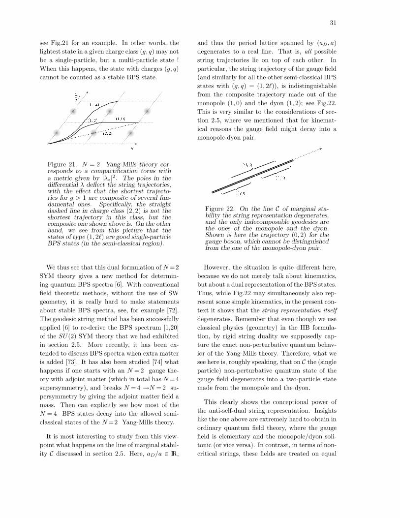
31

see Fig.21 for an example. In other words, the

lightest state in a given charge class (g, q) may not

be a single-particle, but a multi-particle state !

When this happens, the state with charges (g, q)

cannot be counted as a stable BPS state.

(1; 2)(1; 4)g

12q (1; 0)(2; 2)Figure 21. N = 2 Yang-Mills theory cor-responds to a compactification torus witha metric given by |λz|2. The poles in thedifferential λ deflect the string trajectories,with the effect that the shortest trajecto-ries for g > 1 are composite of several fun-damental ones. Specifically, the straightdashed line in charge class (2, 2) is not theshortest trajectory in this class, but thecomposite one shown above is. On the otherhand, we see from this picture that thestates of type (1, 2ℓ) are good single-particleBPS states (in the semi-classical region).

We thus see that this dual formulation of N=2

SYM theory gives a new method for determin-

ing quantum BPS spectra [6]. With conventional

field theoretic methods, without the use of SW

geometry, it is really hard to make statements

about stable BPS spectra, see, for example [72].

The geodesic string method has been successfully

applied [6] to re-derive the BPS spectrum [1,20]

of the SU(2) SYM theory that we had exhibited

in section 2.5. More recently, it has been ex-

tended to discuss BPS spectra when extra matter

is added [73]. It has also been studied [74] what

happens if one starts with an N = 2 gauge the-

ory with adjoint matter (which in total has N=4

supersymmetry), and breaks N = 4 →N = 2 su-

persymmetry by giving the adjoint matter field a

mass. Then can explicitly see how most of the

N = 4 BPS states decay into the allowed semi-

classical states of the N=2 Yang-Mills theory.

It is most interesting to study from this view-

point what happens on the line of marginal stabil-

ity C discussed in section 2.5. Here, aD/a ∈ IR,

and thus the period lattice spanned by (aD, a)

degenerates to a real line. That is, all possible

string trajectories lie on top of each other. In

particular, the string trajectory of the gauge field

(and similarly for all the other semi-classical BPS

states with (g, q) = (1, 2ℓ)), is indistinguishable

from the composite trajectory made out of the

monopole (1, 0) and the dyon (1, 2); see Fig.22.

This is very similar to the considerations of sec-

tion 2.5, where we mentioned that for kinemat-

ical reasons the gauge field might decay into a

monopole-dyon pair.

Figure 22. On the line C of marginal sta-bility the string representation degenerates,and the only indecomposable geodesics arethe ones of the monopole and the dyon.Shown is here the trajectory (0, 2) for thegauge boson, which cannot be distinguishedfrom the one of the monopole-dyon pair.

However, the situation is quite different here,

because we do not merely talk about kinematics,

but about a dual representation of the BPS states.

Thus, while Fig.22 may simultaneously also rep-

resent some simple kinematics, in the present con-

text it shows that the string representation itself

degenerates. Remember that even though we use

classical physics (geometry) in the IIB formula-

tion, by rigid string duality we supposedly cap-

ture the exact non-perturbative quantum behav-

ior of the Yang-Mills theory. Therefore, what we

see here is, roughly speaking, that on C the (single

particle) non-perturbative quantum state of the

gauge field degenerates into a two-particle state

made from the monopole and the dyon.

This clearly shows the conceptional power of

the anti-self-dual string representation. Insights

like the one above are extremely hard to obtain in

ordinary quantum field theory, where the gauge

field is elementary and the monopole/dyon soli-

tonic (or vice versa). In contrast, in terms of non-

critical strings, these fields are treated on equal

32

footing [39]. Other applications of this dual rep-

resentation of N = 2 gauge theory include the

description of non-abelian gauge flux tubes and

confinement in terms of non-critical strings [75].

6. Conclusions

Note that the above construction of the SW

theory is deductive – the SW theory in its full

glory can be systematically derived from string

theory, once one takes the heterotic-type II string

duality [2] for granted and works out its conse-

quences. This convergent evolution of a priori

disparate physical ideas seems to indicate that

we are really on the right track for understanding

non-perturbative phenomena in supersymmetric

field and string theory.

Acknowledgements

I like to thank S. Kachru, A. Klemm, P. Mayr,

S. Theisen, C. Vafa, N. Warner and S. Yankielow-

icz for pleasant collaboration, and K. Pilch for

comments on the manuscript. I also thank the

organizers of the school for their hard work.

REFERENCES

1. N. Seiberg and E. Witten, Nucl. Phys. B426

(1994) 19, hep-th/9407087; Nucl. Phys. B431

(1994) 484, hep-th/9408099.

2. C. Hull and P. Townsend, Nucl. Phys. B438

(1995) 109, hep-th/9410167.

3. See eg.,

E. Witten, as in [39];

P. K. Townsend, P-brane Democracy, hep-

th/9507048;

K. & M. Becker and A. Strominger,

Nucl. Phys. B456 (1995) 130-152, hep-

th/9507158;

J. Polchinski, Phys. Rev. Lett. 75 (1995)

4724-4727, hep-th/9510017;

Cumrun Vafa, Nucl. Phys. B469 (1996) 403-

418, hep-th/9602022.

D. Kutasov and E. Martinec, New Princi-

ples for String/Membrane Unification, hep-

th/9602049;

M. Green, World-volumes and string target

spaces, hep-th/9602061.

4. A. Bilal, Duality in N=2 SUSY SU(2) Yang-

Mills Theory: A pedagogical introduction

to the work of Seiberg and Witten, hep-

th/9601007;

C. Gomez and R. Hernandez, Electric-

Magnetic Duality and Effective Field The-

ories, hep-th/9510023; C. Gomez, R. Her-

nandez and E. Lopez, Integrability, Duality

and Strings, hep-th/9604043, Integrability,

Jacobians and Calabi-Yau Threefolds, hep-

th/9604057;

L. Alvarez-Gaume and M. Marino, to appear.

5. See e.g., V. Arnold, A. Gusein-Zade and

A. Varchenko, Singularities of Differentiable

Maps I, II, Birkhauser 1985;

V. Arnold, Dynamical Systems VI, Singu-

larity Theory I, Enc. of Math. Sci. Vol. 6,

Springer 1993.

6. A. Klemm, W. Lerche, P. Mayr, C. Vafa and

N. Warner, Self-Dual Strings and N=2 Super-

symmetric Field Theory, hep-th/9604034.

7. A. Gorskii, I. Krichever, A. Marshakov, A.

Mironov and A. Morozov, Phys. Lett. B355

(1995) 466-474, hep-th/9505035.

8. N. Seiberg, Phys. Lett. B206 (1988) 75.

9. V. Novikov, M. Schifman, A. Vainstein, M

Voloshin and V. Zakharov, Nucl. Phys. B229

(1983) 394;

V. Novikov, M. Schifman, A. Vainstein and

V. Zakharov, Nucl. Phys. B229 (1983) 381,

407;

M. Schifman, A. Vainstein and V. Zakharov,

Phys. Lett. B166 (1986) 329.

10. E. Witten, Monopoles and Four Manifolds,

hep-th/9411102.

11. D. Finnell and P. Pouliot, Nucl. Phys. B453

(1995) 225-239, hep-th/9503115;

A. Yung, Instanton-induced Effective La-

grangian in the Seiberg-Witten Model, hep-

th/9605096;

K. Ito and N. Sasakura, Phys. Lett. B382

(1996) 95-103, hep-th/9602073;

F. Fucito and G. Travaglini, Instanton Calcu-

lus and Nonperturbative Relations in N =

2 Supersymmetric Gauge Theories, hep-

33

th/9605215;

N. Dorey, V.A. Khoze and M. Mattis, Multi-

Instanton Check of the Relation Between the

Prepotential F and the Modulus u in N = 2

SUSY Yang-Mills Theory, hep-th/9606199;

Phys. Rev. D54 (1996) 2921-2943, hep-

th/9603136; A Two-Instanton Test of the Ex-

act Solution of N = 2 Supersymmetric QCD,

hep-th/9607066; Multi-Instanton Calculus in

N = 2 Supersymmetric Gauge Theory II:

Coupling to Matter, hep-th/9607202;

T. Harano and M. Sato, Multi-Instanton Cal-

culus versus Exact Results in N = 2 Super-

symmetric QCD, hep-th/9608060;

H. Aoyama, T. Harano, M. Sato and S. Wada,

Multi-Instanton Calculus in N = 2 Super-

symmetric QCD, hep-th/9607076.

12. L. Alvarez-Gaume, J. Distler, C. Kounnas

and M. Marino, Large Softly broken N = 2

QCD, hep-th/9604004;

L. Alvarez-Gaume and M. Marino, Softly bro-

ken N = 2 QCD, hep-th/9606168; More on

softly broken N = 2 QCD, hep-th/9606191.

13. D. Olive and E. Witten, Phys. Lett. B78(

1978) 97.

14. See for reviews eg., N. Seiberg, The Power of

holomorphy: Exact results in 4-D SUSY field

theories, hep-th/9408013;

K. Intriligator and N. Seiberg, Lectures

on Supersymmetric Gauge Theories and

Electric-Magnetic Duality, Nucl. Phys. Proc.

Suppl. 45BC (1996) 1-28, hep-th/9509066;

S. Elitzur, A. Forge, A. Giveon and E. Ra-

binovici, Summary of Results in N = 1 Su-

persymmetric SU(2) Gauge Theories, hep-

th/9512140.

15. Mans Henningson, Nucl. Phys. B458 (1996)

445-455, hep-th/9507135;

M. Matone, Modular Invariance and Exact

Wilsonian Action of N = 2 SYM, hep-

th/9610204.

16. R. Flume, M. Magro, L. O’Raifeartaigh, I.

Sachs and O. Schnetz, Uniqueness of the

Seiberg-Witten Effective Lagrangian, hep-

th/9611123.

17. G. ‘t Hooft, Nucl. Phys. B190 (1981) 455.

18. P. Argyres and M. Douglas, as in ref. [25].

19. E. Witten, Phys. Lett. B86 (1979) 283.

20. A. Bilal and F. Ferrari, The Strong-Coupling

Spectrum of the Seiberg-Witten Theory,

Nucl. Phys. B469 (1996) 387-402, hep-

th/9602082.

21. A. Ceresole, R. D’Auria, S. Ferrara, Phys.

Lett. B339 (1994) 71-76, hep-th/9408036;

A. Klemm, W. Lerche and S. Theisen, as in

ref. [25];

S. Ryang, Phys. Lett. B365 (1996) 113-118,

hep-th/9508163;

J. Isidro, A. Mukherjee, J. Nunes and H.

Schnitzer, A New Derivation of the Picard-

Fuchs Equations for Effective N=2 Super

Yang-Mills Theories, hep-th/9609116;

M. Alishahiha, On the Picard-Fuchs equa-

tions of the SW models, hep-th/9609157;

H. Ewen and K. Foerger, Simple Calculation

of Instanton Corrections in Massive N = 2

SU(3)SYM, hep-th/9610049.

22. A. Klemm, W. Lerche and S. Theisen, last

reference in [25].

23. N. Seiberg and E. Witten, as in [1];

A. Hanany and Y. Oz, Nucl. Phys. B452

(1995) 283-312, hep-th/9505075;

P. Argyres, M. Plesser and A. Shapere,

Phys. Rev. Lett. 75 (1995) 1699-1702, hep-

th/9505100;

J. Minahan and D. Nemeschansky, Nucl.

Phys. B464 (1996) 3-17, hep-th/9507032;

Nucl. Phys. B468 (1996) 72-84, hep-

th/9601059;

R. Donagi and E. Witten, Nucl. Phys. B460

(1996) 299-334, hep-th/9510101;

P. Argyres and A. Shapere, Nucl. Phys. B461

(1996) 437-459, hep-th/9509175;

A. Hanany, Nucl. Phys. B466 (1996) 85-100,

hep-th/9509176;

P. Argyres, M. Plesser and N. Seiberg, Nucl.

Phys. B471 (1996) 159-194, hep-th/9603042;

K. Ito and S.K. Yang, Picard-Fuchs Equa-

tions and Prepotentials in N = 2 Supersym-

metric QCD, hep-th/9603073;

A. Bilal and F. Ferrari, Exact Multiplets of

Spontaneously Broken Discrete Global Sym-

metries: The Example of N = 2 SUSY QCD,

hep-th/9606111;

F. Ferrari, Charge fractionization in N = 2

supersymmetric QCD, hep-th/9609101;

34

A. Brandhuber and S. Stieberger, Periods,

Coupling Constants and Modular Functions

in N = 2 SU(2) SYM with Massive Matter,

hep-th/9609130;

N. Dorey, V. Khoze and M. Mattis, OnN = 2

Supersymmetric QCD with 4 Flavors, hep-

th/9611016.

24. K. Ito and S.K. Yang, Picard-Fuchs Equa-

tions and Prepotentials in N = 2 Supersym-

metric QCD, hep-th/9603073;

Y. Ohta, Prepotential of N = 2 SU(2) Yang-

Mills Gauge Theory Coupled with a Massive

Matter Multiplet, hep-th/9604051; Prepoten-

tial of N = 2 SU(2) Yang-Mills Gauge The-

ory Coupled with Massive Matter Multiplets,

hep-th/9604059;

T. Masuda and H. Suzuki, Prepotential of

N = 2 Supersymmetric Yang-Mills The-

ories in the Weak Coupling Region, hep-

th/9609065; Periods and Prepotential of

N=2 SU(2) Supersymmetric Yang- Mills

Theory with Massive Hypermultiplets, hep-

th/9609066;

H. Ewen, K. Forger and S. Theisen, Prepoten-

tials in N = 2 Supersymmetric SU(3) YM-

Theory with Massless Hypermultiplets, hep-

th/9609062.

25. A. Klemm, W. Lerche, S. Theisen and S.

Yankielowicz, Phys. Lett. B344 (1995) 169,

hep-th/9411048;

P. Argyres and A. Faraggi, Phys. Rev. Lett.

74 (1995) 3931, hep-th/9411057;

M. Douglas and S. Shenker, Nucl. Phys.

B447 (1995) 271, hep-th/9503163;

P. Argyres and M. Douglas, Nucl. Phys.

B448 (1995) 93, hep-th/9505062;

A. Klemm, W. Lerche and S. Theisen, Int.

J. Mod. Phys. A11 (1996) 1929-1974, hep-

th/9505150;

C. Fraser and T. Hollowood, On the Weak

Coupling Spectrum of N = 2 Supersymmet-

ric SU(n) Gauge theory, hep-th/9610142.

26. U. Danielsson and B. Sundborg, Phys. Lett.

B358 (1995) 273, hep-th/9504102;

A. Brandhuber and K. Landsteiner, Phys.

Lett. B358 (1995) 73, hep-th/9507008;

U. Danielsson and B. Sundborg, Phys. Lett.

B370 (1996) 83-94, hep-th/9511180;

M. Alishahiha, F. Ardalan and F. Man-

souri, Phys. Lett. B381 (1996) 446-450, hep-

th/9512005; M. R. Abolhasani, M. Alishahiha

and A. M. Ghezelbash, The Moduli Space and

Monodromies of the N = 2 Supersymmet-

ric Yang-Mills Theory with any Lie Gauge

Groups, hep-th/9606043;

W. Lerche and N. Warner, Exceptional

SW Geometry from ALE Fibrations, hep-

th/9608183;

K. Landsteiner, J. Pierre and S. Giddings, On

the Moduli Space of N = 2 Supersymmetric

G2 Gauge Theory, hep-th/9609059.

27. E. Martinec and N.P. Warner, Nucl. Phys.

B459 (1996) 97-112, hep-th/9509161.

28. see eg., P. Slodowy, Platonic Solids, Kleinian

Singularities and Lie Groups, in: Algebraic

Geometry, Lecture Notes in Mathematics

1008, Springer 1983.

29. W. Lerche and N. P. Warner, as in [26].

30. P. Argyres, M. Plesser and N. Seiberg and E.

Witten, Nucl. Phys. B461 (1996) 71-84, hep-

th/9511154;

T. Eguchi, K. Hori, K. Ito and S.K. Yang,

Nucl. Phys. B471 (1996) 430-444, hep-

th/9603002.

31. M. Matone, Phys. Lett. B357 (1995) 342-

348, hep-th/9506102;

J. Sonnenschein, S. Theisen and S. Yankie-

lowicz, Phys. Lett. B367 (1996) 145-150,

hep-th/9510129;

T. Eguchi and S.K. Yang, Prepotentials of

N = 2 Supersymmetric Gauge Theories and

Soliton Equations, hep-th/9510183;

H. Itoyama and A. Morozov, Prepotential and

the Seiberg-Witten Theory, hep-th/9512161;

G. Bonelli and M. Matone, Phys. Rev. Lett.

76 (1996) 4107-4110, hep-th/9602174; Non-

perturbative Relations in N = 2 Susy Yang-

Mills and WDVV Equation, hep-th/9605090.

32. A. Klemm, W. Lerche, S. Theisen and S.

Yankielowicz, first reference in [25].

33. P. Argyres and A. Faraggi, as in [25].

34. E. D’Hoker, I. Krichever and D. Phong,

The Effective Prepotential of N = 2 Su-

persymmetric SU(Nc) Gauge Theories, hep-

th/9609041; The Effective Prepotential of

N = 2 Supersymmetric SO(Nc) and Sp(Nc)

35

Gauge Theories, hep-th/9609145.

35. T. Nakatsu and K. Takasaki, Mod. Phys.

Lett. A11 (1996) 157-168, hep-th/9509162;

E. Martinec, Phys. Lett. B367 (1996) 91-96,

hep-th/9510204;

H. Itoyama and A. Morozov, Integrability

and Seiberg-Witten Theory: Curves and Pe-

riods, hep-th/9511126; Prepotential and the

Seiberg-Witten Theory, hep-th/9512161; In-

tegrability and Seiberg-Witten theory, hep-

th/9601168;

I. Krichever and D. Phong, On the Inte-

grable Geometry of Soliton Equations and

N = 2 Supersymmetric Gauge Theories, hep-

th/9604199;

A. Gorskii, Peierls model and Vacuum Struc-

ture in N = 2 Supersymmetric Gauge Theo-

ries, hep-th/9605135;

A. Marshakov, A. Mironov and A. Morozov,

WDVV-like equations in N = 2 SUSY Yang-

Mills Theory, hep-th/9607109;

A. Marshakov, From Nonperturbative SUSY

Gauge Theories to Integrable Systems, hep-

th/9607159; Integrability as Effective Prin-

ciple of Nonperturbative Field and String

Theories, hep-th/9608161; Non-perturbative

Quantum Theories and Integrable Equations,

hep-th/9610242;

36. P. Aspinwall and M. Gross, The SO(32)

Heterotic String on a K3 Surface, hep-

th/9605131.

37. W. Nahm, On the Seiberg-Witten Approach to

electric-magnetic Duality, hep-th/9608121.

38. M. Bershadsky, V. Sadov and C. Vafa,

Nucl. Phys. B463 (1996) 398-414, hep-

th/9510225.

39. E. Witten, Some Comments on String Dy-

namics, hep-th/9507121.

40. M. Duff and J. Lu, Nucl. Phys. B416 (1994)

301, hep-th/9306052;

N. Seiberg and E. Witten, Nucl. Phys. B471

(1996) 121-134, hep-th/9603003;

M. J. Duff, H. Lu and C. N. Pope, Phys.

Lett. B378 (1996) 101-106, hep-th/9603037;

E. Witten, Nucl. Phys. B471 (1996) 195-216,

hep-th/9603150;

P. Argyres and K. Dienes, Phys. Lett. B387

(1996) 727-734, hep-th/9607190;

M. Perry and J. Schwarz, Interacting Chiral

Gauge Fields in Six Dimensions and Born-

Infeld Theory, hep-th/9611065;

J. Distler and A. Hanany, (0,2) Noncritical

Strings in Six Dimensions, hep-th/9611104.

41. S. Kachru and C. Vafa, Nucl. Phys. B450

(1995) 69, hep-th/9506024.

42. S. Ferrara, J. Harvey, A. Strominger and

C. Vafa, Phys. Lett. B361 (1995) 59, hep-

th/9505162.

43. P. Aspinwall, K3 Surfaces and String Duality,

hep-th/9611137.

44. W. Lerche, A. N. Schellekens and N. P.

Warner, Lattices and Strings, Phys. Rept.

177 (1989) 1.

45. E. Witten, Nucl. Phys. B443 (1995) 85, hep-

th/9503124.

46. P. Aspinwall, Phys. Lett. B357 (1995) 329-

334, hep-th/9507012.

47. M. Douglas and G. Moore, D-branes, Quivers,

and ALE Instantons, hep-th/9603167.

48. T. Eguchi and A. Hanson, Phys. Lett. B74

(1978) 249.

49. A. Sen, F-theory and Orientifolds, hep-

th/9605150;

T. Banks, M. Douglas and N. Seiberg, Prob-

ing F-theory with Branes, hep-th/9605199;

K. Dasgupta and S. Mukhi, F-theory at Con-

stant Coupling, hep-th/9606044.

50. M. Douglas and M. Li, D-Brane Realization

of N = 2 Super Yang-Mills Theory in Four

Dimensions, hep-th/9604041.

51. S. Yau (ed.), Essays on Mirror Manifolds, In-

ternational Press 1992.

52. V. Kaplunovsky, J. Louis, and S. Theisen,

Phys. Lett. B357 (1995) 71-75, hep-

th/9506110;

A.Klemm, W. Lerche and P. Mayr, as in [60];

C. Vafa and E. Witten,as in [61];

G. Cardoso, D. Lust and T. Mohaupt, hep-

th/9507113;

I. Antoniadis, E. Gava, K. Narain and T.

Taylor, Nucl. Phys. B455 (1995) 109, hep-

th/9507115;

S. Kachru, A. Klemm, W. Lerche, P. Mayr

and C. Vafa, as in [76];

A. Sen and C. Vafa, Nucl. Phys. B455 (1995)

165-187, hep-th/9508064.

36

I. Antoniadis and H. Partouche, Nucl. Phys.

B460 (1996) 470, hep-th/9509009;

G. Curio, Phys. Lett. B366 (1996) 131, hep-

th/9509042; Phys. Lett. B368 (1996) 78,

hep-th/9509146;

G. Aldazabal, A. Font, L.E. Ibanez and F.

Quevedo, hep-th/9510093;

I. Antoniadis, S. Ferrara, E. Gava, K. Narain

and T. Taylor, Nucl. Phys. Proc. Suppl.

45BC (1996) 177-187, hep-th/9510079;

P. Aspinwall, Nucl. Phys. B460 (1996) 57-

76, hep-th/9510142;

J. Harvey, G. Moore, Algebras, BPS States,

and Strings, Nucl. Phys. B463 (1996) 315-

368, hep-th/9510182;

P. Aspinwall and J. Louis, as in [62];

I. Antoniadis, S. Ferrara and T. Taylor,Nucl.

Phys. B460 (1996) 489, hep-th/9511108;

M. Henningson and G. Moore, Nucl. Phys.

B472 (1996) 518-528, hep-th/9602154;

G. Cardoso, G. Curio, D. Lust and T Mo-

haupt, Instanton Numbers and Exchange

Symmetries in N = 2 Dual String Pairs, hep-

th/9603108;

P. Candelas and A. Font, Duality Between

Webs of Heterotic and Type II Vacua, hep-

th/9603170;

I. Antoniadis, E. Gava, K. Narain and T. Tay-

lor, Topological Amplitudes in Heterotic Su-

perstring Theory, hep-th/9604077;

J. Louis, J. Sonnenschein, S. Theisen and

S. Yankielowicz, Non-Perturbative Properties

of Heterotic String Vacua Compactified on

K3 × T 2, hep-th/9606049;

I. Antoniadis and B. Pioline, Higgs branch,

HyperKaehler Quotient and Duality in SUSY

N = 2 Yang-Mills Theories, hep-th/9607058;

C. Gomez, R. Hernandez and E. Lopez, K3-

Fibrations and Softly Broken N = 4 Super-

symmetric Gauge Theories, hep-th/9608104;

G. Cardoso, G. Curio and D. Lust, Perturba-

tive Couplings and Modular Forms in N =

2 String Models with a Wilson Line, hep-

th/9608154;

J. Harvey and G. Moore, Fivebrane Instan-

tons and R2 couplings in N = 4 String The-

ory, hep-th/9610237.

53. C. Vafa, Nucl. Phys. B469 (1996) 403-418,

hep-th/9602022;

D. Morrison and C. Vafa, Nucl. Phys. B473

(1996) 74-92, hep-th/9602114; Compactifica-

tions of F-Theory on Calabi–Yau Threefolds

– II, hep-th/9603161.

54. B. de Wit, P. Lauwers, R. Philippe, S. Su and

A. van Proeyen, Phys. Lett. B134 (1984)37;

B. de Wit, A. van Proeyen, Nucl. Phys. B245

(1984)89;

J.P. Derendinger, S. Ferrara, A. Masiero and

A. van Proeyen, Phys. Lett. B140 (1984)307;

B. de Wit, P.G. Lauwers, A. van Proeyen,

Nucl. Phys. B255 (1985)569;

E. Cremmer, C. Kounnas, A. van Proeyen,

J.P. Derendinger, S. Ferrara, B. de Wit and

L. Girardello, Nucl. Phys. B250 (1985)385;

N. Berkovits and W. Siegel, Nucl. Phys. B462

(1996)213.

55. P. Candelas, X. De La Ossa, P. Green and L.

Parkes, Nucl. Phys. B359 (1991) 21-74;

S. Hosono, A. Klemm and S. Theisen, Lec-

tures on Mirror Symmetry, hep-th/9403096.

56. A. Strominger, Nucl. Phys. B451 (1995) 96,

hep-th/9504090;

B. Greene, D. Morrison and A. Stro-

minger, Nucl. Phys. B451 (1995) 109, hep-

th/9504145.

57. A. Strominger, Black Hole Condensation and

Duality in String Theory, hep-th/9510207.

58. S. Ferrara and A. Strominger, N = 2 Space-

Time Supersymmetry and Calabi-Yau Moduli

Space, in Strings ’89, eds. R. Arnowitt et al.

(World Scientific, 1989) p.245;

A. Strominger, Comm. Math. Phys 133

(1990) 163-180;

L. Dixon, V. Kaplunovsky and J. Louis, Nucl.

Phys. B329, (1993) 27;

L. Castellani, R. D’Auria and S. Ferrara,

Phys. Lett. B241,(1990) 57.

59. A. Ceresole, R. D’Auria, S. Ferrara and A.

Van Proeyen, Nucl. Phys. B444 (1995) 92,

hep-th/9502072;

B. de Wit, V. Kaplunovsky, J. Louis and D.

Lust, Perturbative Couplings of Vector Mul-

tiplets in N = 2 Heterotic String Vacua, hep-

th/9504006;

I. Antoniadis, S. Ferrara, E. Gava, K. Narain

and T. Taylor, Nucl. Phys. B447 (1995) 35-

37

61, hep-th/9504034;

M. Billo, A. Ceresole, R. D’Auria, S. Fer-

rara, P. Fre, T. Regge, P. Soriani, and A. Van

Proeyen, Class. Quant. Grav. 13 (1996) 831-

864, hep-th/9506075;

G. Cardoso, D. Lust and T. Mohaupt,

Nucl. Phys. B455 (1995) 131-164, hep-

th/9507113;

S. Kachru, A. Klemm, W. Lerche, P. Mayr

and C. Vafa, as in [76].

60. A. Klemm, W. Lerche and P. Mayr, Phys.

Lett. B357 (1995) 313-322, hep-th/9506112.

61. C. Vafa and E. Witten, Dual String Pairs

With N = 1 And N = 2 Supersymmetry In

Four Dimensions, hep-th/9507050.

62. P. Aspinwall and J. Louis, Phys. Lett. B369

(1996) 233-242, hep-th/9510234;

P. Aspinwall and M. Gross, Phys. Lett. B382

(1996) 81-88, hep-th/9602118.

63. B. Hunt and R. Schimmrigk, Phys. Lett.

B381 (1996) 427-436, hep-th/9512138;

S. Hosono, B. Lian and S. T. Yau, Calabi-

Yau Varieties and Pencils of K3 Surfaces, alg-

geom/9603020;

A. C. Avram, M. Kreuzer, M. Mandelberg

and H. Skarke, Searching for K3 Fibrations,

hep-th/9610154.

64. S. Katz, A. Klemm and C. Vafa, Geometric

Engineering of Quantum Field Theories, hep-

th/9609239.

65. S. Katz and C. Vafa, Matter from Geometry,

hep-th/9606086;

M. Bershadsky et. al., Geometric Singulari-

ties and Enhanced Gauge Symmetries, hep-

th/9605200.

66. A. Klemm, W. Lerche, P. Mayr and N.

Warner, unpublished and perhaps to appear.

67. A. Klemm and P. Mayr, Strong Coupling Sin-

gularities and Non-abelian Gauge Symmetries

in N = 2 String Theory, hep-th/9601014;

S. Katz, D. Morrison and M. Plesser,

Nucl. Phys. B477 (1996) 105-140, hep-

th/9601108.

68. E. Witten, Nucl. Phys. B460 (1996) 541-

559, hep-th/9511030.

69. E. Verlinde, Nucl. Phys. B455 (1995) 211,

hep-th/9506011.

70. A. Ceresole, R. D’Auria, S. Ferrara and A.

Van Proeyen, as in ref. [59];

S. Ferrara, R. Minasian and A. Sagnotti,

Nucl. Phys. B474 (1996) 323-342, hep-

th/9604097.

71. K. & M. Becker and A. Strominger, as in ref.

[3].

72. A. Sen, Phys. Lett. B329 (1994) 217, hep-

th/9402032;

S. Sethi, M. Stern, and E. Zaslow, Nucl. Phys.

B457 (1995) 484, hep-th/9508117;

J. Gauntlett and J. Harvey, preprint EFI-95-

56, hep-th/9508156.

73. A. Brandhuber and S. Stieberger, Self-Dual

Strings and Stability of BPS States in N = 2

SU(2) Gauge Theories, hep-th/9610053.

74. J. Schulze and N. Warner, to appear.

75. B. Greene, D. Morrison and C. Vafa, A

Geometric Realization of Confinement, hep-

th/9608039.

76. S. Kachru, A. Klemm, W. Lerche, P. Mayr

and C. Vafa, Nucl. Phys. B459 (1996) 537,

hep-th/9508155.