Embed Size (px)
Citation preview

arX
iv:h
ep-t
h/04
1100
4v2
27
Feb
2005
Mechanics and Newton-Cartan-Like Gravity on the Newton-Hooke
Space-time
Yu Tian1,∗ Han-Ying Guo2,1,† Chao-Guang Huang3,‡ Zhan Xu4,§ and Bin Zhou5,6¶
1 Institute of Theoretical Physics, Chinese Academy of Sciences,P.O. Box 2735, Beijing 100080, China
2 CCAST (World Laboratory), P.O. Box 8730, Beijing 100080, China3 Institute of High Energy Physics, Chinese Academy of Sciences,
P.O. Box 918-4, Beijing 100049, China4 Physics Department, Tsinghua University, Beijing 100084, China
5 Physics Department, Beijing Normal University, Beijing 100875, China and6 Interdisciplinary Center of Theoretical Studies,
Chinese Academy of Sciences, Beijing 100080, China(Dated: October 13, 2018)
AbstractWe focus on the dynamical aspects on Newton-Hooke space-time NH+ mainly from the viewpoint of ge-
ometric contraction of the de Sitter spacetime with Beltrami metric. (The term spacetime is used to denote
a space with non-degenerate metric, while the term space-time is used to denote a space with degenerate
metric.) We first discuss the Newton-Hooke classical mechanics, especially the continuous medium mechan-
ics, in this framework. Then, we establish a consistent theory of gravity on the Newton-Hooke space-time as
a kind of Newton-Cartan-like theory, parallel to the Newton’s gravity in the Galilei space-time. Finally, we
give the Newton-Hooke invariant Schrodinger equation from the geometric contraction, where we can relate
the conservative probability in some sense to the mass density in the Newton-Hooke continuous medium
mechanics. Similar consideration may apply to the Newton-Hooke space-time NH− contracted from anti-de
Sitter spacetime.
PACS numbers: 04.20.Cv, 45.20.-d, 02.40.Dr
∗Electronic address: [email protected]†Electronic address: [email protected]‡Electronic address: [email protected]§Electronic address: [email protected]¶Electronic address: [email protected]
1

Contents
I. Introduction 3
II. Newton-Hooke Space-time as a Limit of Beltrami-de Sitter Spacetime 4A. Hyperboloid Model of de Sitter Spacetime 5B. Beltrami-de Sitter Model 6
1. Beltrami Coordinates 62. Fractional Linear Form of de Sitter Group 7
C. The Newton-Hooke Limit 7
III. Newton-Hooke Classical Mechanics 9A. Newton-Hooke Kinematics 9B. Newton-Hooke Dynamics 10C. On Newton-Hooke Continuous Medium Mechanics 11
IV. Newton-Cartan-Like Theory on the Newton-Hooke Space-time 12A. Physical Requirements and Gravitational Field Equation 13B. Law of Gravity for Spherical Source 14
V. Schrodinger Equation on the Newton-Hooke Space-time 15A. Schrodinger Equation from Geometric Contraction 15B. Conservation of Probability 16
VI. Conclusion and Discussion 17
Acknowledgments 17
A. Newton-Hooke Invariant Connection 17
B. Energy in Newton-Hooke Mechanics 19
C. Transformation Property of Γ ktt 19
D. Schrodinger Equation from Algebraic Viewpoint 20
References 20
2
I. INTRODUCTION
From the viewpoint of purely theoretical and fundamental physics, it is well known that thereare eight types of possible kinematical symmetry groups based on some rather natural assumptions[1]. Among them the most basic two are de Sitter (dS) and anti-de Sitter (AdS) groups, which areSO(1, d+ 1) and SO(2, d) for (1 + d)-dimensional spacetime, respectively; all the others are Inonu-Wigner contractions [2] of them. The so-called Newton-Hooke (NH) group N± is an important andinteresting contraction of dS/AdS group, respectively. It is the meaningful non-relativistic limitof dS/AdS group. At the same time, the Galilei group is a further contraction (the flat limit) ofboth N± groups. All these kinematical groups can lead to the corresponding (1 + d)-dimensionalspace-times as some homogeneous spaces of them. Furthermore, the action of these groups ontheir corresponding space-times can take some nice fractional linear forms under special coordinatesystems (called Beltrami coordinates1), and the corresponding mechanics, like Newtonian mechanicson Galilei space-time, can be really established from first principles [3, 4]. Especially, the NH caseas a non-relativistic cosmological kinematics is studied in detail in [5] and recently in [3].
On the other hand, from the viewpoint of modern physics and cosmology, constant curvaturespace-times have drawn much attention, from both theoretical and observational considerations.The significance of AdS space is early recognized, based upon the fact that its symmetry algebrahas supersymmetric extensions and so it can be incorporated into supergravity and string theory.Related study has resulted in the profound AdS/CFT correspondence [6]. The great interest in dSspace comes from recent cosmological observations showing that our universe is asymptotic dS, i.e.,with a positive cosmological constant [7, 8]. However, there will be lots of puzzles within the presentframework of physics if our universe does have a positive cosmological constant [9]. Under thisembarrassed situation, of course, any instructive attempts related to these problems are worthwhile.One available attempt is just to consider the non-relativistic limit, i.e., the NH limit, which drasticallysimplifies the analysis while still taking the effects of cosmological constant into account. That iswhy the interest in NH space-time revives recent years [3, 10–12].
Following our recent paper [3] that investigates NH space-time from the geometric contraction,in this paper we focus on the dynamical aspects on NH space-time. We discuss in detail the NHkinematics, dynamics and even continuous medium mechanics. Especially, we establish a consistenttheory of gravity on NH space-time as a kind of Newton-Cartan-like theory, parallel to the Newton’sgravity on the Galilei space-time. We also discuss some interesting aspects of the NH invariantSchrodinger equation. We find that it is possible to relate the conservative probability in some senseto the mass density in the NH continuous medium mechanics. Unlike most of preceding articles,which investigate NH mechanics mainly from the algebraic point of view, our discussion will be moregeometric and based on the foundation of physics. The invariance of physics under the action of NHgroup plays an important role in our discussion.
The paper is organized as follows. In Sec.II, after a brief introduction to algebraic construction ofNH space-time, we introduce the geometric description of dS/AdS spacetime, Beltrami coordinates,dS/AdS group action and their NH limit for the dS spacetime. In Sec.III we discuss the NH mechan-ics, concentrating on the dynamics. The Newton-Cartan-like theory on NH space-time is constructedin Sec.IV. We give the gravitational field equation there and solve it to obtain the law of gravityfor the exterior of spherical source. In Sec.V we deduce the Schrodinger equation on NH space-timefrom the geometric contraction, show its NH invariance, and discuss the conservation of probability,which can be related in some sense to the mass density in fluid mechanics. We end the paper witha brief conclusion and discussion in Sec.VI.
1 Cartesian coordinates on the (pseudo-)Euclidean spaces, actually, are the limiting case under contraction of Beltrami
coordinates.
3

II. NEWTON-HOOKE SPACE-TIME AS A LIMIT OF BELTRAMI-DE SITTER SPACE-
TIME
The Lie algebra of dS/AdS group, in terms of the time-space decomposition, is (taking d = 3 fordefiniteness) [3]
[Ji,H] = 0, [Ji,Jj] = ǫijkJk, [Ji,Pj] = ǫijkPk,
[Ji,Kj] = ǫijkKk, [H,Pi] = ±ν2Ki, [H,Ki] = Pi, (2.1)
[Pi,Pj] = ±R−2ǫijkJk, [Ki,Kj] = −c−2ǫijkJk, [Pi,Kj] = c−2δijH,
where the generators have their usual meanings, ν := c/R has the same dimension as frequency,and the “+”/“−” sign is for dS/AdS, respectively. The Newton-Hooke (NH) algebra n±(1, 3) is thefollowing limit (contraction) of the above dS/AdS algebra:
c→ ∞, R → ∞, but ν =c
Ris a positive, finite constant, (2.2)
which reads
[Ji,Jj ] = ǫijkJk, [Ji,Pj] = ǫijkPk,
[Ji,Kj] = ǫijkKk, [H,Pi] = ±ν2Ki, [H,Ki] = Pi, (2.3)
and the other Lie brackets vanish.
If we first replace H with H− imc2, where m is a central element, and then perform the contraction,we will get the central extension nC±(1, 3) of NH algebra (2.3):
[Ji,Jj ] = ǫijkJk, [Ji,Pj] = ǫijkPk,
[Ji,Kj] = ǫijkKk, [H,Pi] = ±ν2Ki, [H,Ki] = Pi, (2.4)
[Pi,Kj] = −iδijm, and the other Lie brackets vanish.
From the spacetime point of view, the parameter R in eq.(2.1) is the cosmic radius, which is relatedto the cosmological constant Λ by Λ = ±3R−2. Now in the NH limit the new parameter ν takes itsplace and has the meaning of temporal curvature. If we perform a further contraction ν → 0 (theso-called flat limit) the algebras n± and nC± come back to the familiar Galilei algebra gal and the
corresponding central extension galC, respectively. The algebra galC is well known as the symmetryof non-relativistic quantum mechanics (Schrodinger equation). And it can be seen there that thecentral element m corresponds to the mass.
The above statements on the NH limit is from the Lie algebra point of view (or after exponentiat-ing, from the Lie group point of view). But the group aspects are far from sufficiency. The geometricaspects, such as connections, metrics (if exist) etc, are very important when concerning physics onthese space-times. Conventionally, the next step is to consider dS and AdS spacetimes and NHspace-time as homogeneous spaces SO(1, d+1)/SO(1, d), SO(2, d)/SO(1, d) and N±(1, d)/N±(1, d),respectively, while considering the original groups as the corresponding principal bundles over them.Here N±(1, d) is the homogeneous NH group, whose Lie algebra is the subalgebra of n±(1, d) gen-erated by Ji and Ki.
2 Then one can examine the actions of dS, AdS and NH groups on thesehomogeneous spaces. In this picture the invariant connections on these spaces can be systematicallyobtained as the so-called “canonical” connections [10, 13]. However, this picture does not help usestablish the NH dynamics when taking into account the gravity from matter.
2 In fact, it is easy to see that N±(1, d) and the homogeneous Galilei group are both isomorphic to SO(d) ⊗S Rd.
4
Fortunately, the dS/AdS spacetime has a simple geometric description as the pseudo-sphere em-bedded in higher dimensional Minkowski spacetime. The NH space-time NH± can be directlyobtained as some appropriate limit of this geometric picture. In fact, this naive limiting procedurecan give us all the necessary geometric information of NH space-time. So, from now on, we canforget the algebraic construction of NH space-time and study NH± directly from a geometric pointof view. In the following, we only consider the dS case and the corresponding NH+ (denoted byNH for briefness). NH− can be dealt with in parallel.
A. Hyperboloid Model of de Sitter Spacetime
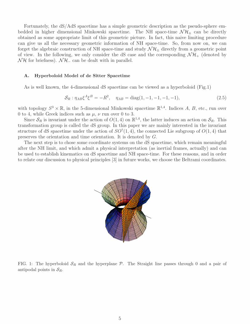
As is well known, the 4-dimensional dS spacetime can be viewed as a hyperboloid (Fig.1)
SR : ηABξAξB = −R2, ηAB = diag(1,−1,−1,−1,−1), (2.5)
with topology S3 × R, in the 5-dimensional Minkowski spacetime R1,4. Indices A, B, etc., run over
0 to 4, while Greek indices such as µ, ν run over 0 to 3.Since SR is invariant under the action of O(1, 4) on R
1,4, the latter induces an action on SR. Thistransformation group is called the dS group. In this paper we are mainly interested in the invariantstructure of dS spacetime under the action of SO↑(1, 4), the connected Lie subgroup of O(1, 4) thatpreserves the orientation and time orientation. It is denoted by G.
The next step is to chose some coordinate systems on the dS spacetime, which remain meaningfulafter the NH limit, and which admit a physical interpretation (as inertial frames, actually) and canbe used to establish kinematics on dS spacetime and NH space-time. For these reasons, and in orderto relate our discussion to physical principles [3] in future works, we choose the Beltrami coordinates.
FIG. 1: The hyperboloid SR and the hyperplane P. The Straight line passes through 0 and a pair of
antipodal points in SR.
5

B. Beltrami-de Sitter Model
1. Beltrami Coordinates
Now let P+4 be the hyperplane ξ4 = R in R
1,4. For each point ξ ∈ SR with ξ4 > 0, there is aone-to-one-corresponding point x ∈ P+
4 such that
ξµx = Rξµ
ξ4=: xµ, ξ4x = R. (2.6)
This map is actually obtained by drawing a straight line passing through ξ and 0 ∈ R1,4, as shown
in Fig.1. Since ξ ∈ SR satisfies eq.(2.5), the corresponding x in P+4 satisfies
σ(x) > 0, (2.7)
whereσ(x) = 1−R−2ηµνx
µxν . (2.8)
The above “gnomonic” projection from SR with ξ4 > 0 into P+4 defines a coordinate system on a
patch, denoted U+4 , of SR, which is known as a Beltrami coordinate system [3, 14, 15]. Note that
in order to preserve the orientation, the antipodal identification should not been taken. Under theBeltrami coordinates, the metric on SR has the form
ds2 = [ηµνσ−1(x) +R−2ηµρηνσx
ρxσσ−2(x)]dxµdxν . (2.9)
We also give the Christoffel connection
Γ ρµν =
xµδρν + xνδ
ρµ
R2σ(x)(2.10)
of this metric for later reference.The patch U+
4 covers almost half of SR. The other half is almost covered by another patch U−4 ,
which is the “gnomonic” projection from SR with ξ4 < 0 into the hyperplane P−4 located at ξ4 = −R
in R1,4. The Beltrami coordinates on U−
4 is given by
xµ = −Rξµ
ξ4. (2.11)
Obviously, there are at least eight patches U±α , α = 1, · · · , 4 to cover the whole SR. In patches
U±α , α = 1, 2, 3, the Beltrami coordinates are given by
xν = ±Rξν
ξα, ν = 0, · · · , α, · · · , 4, ξα ≷ 0, (2.12)
where α means omission of α. In the following discussions, we mainly concentrate on the U+4 patch.
The 3-dimensional hyperboloidσ(x) = 0 (2.13)
is a part of the projective boundary of SR [4], which corresponds to the conformal boundary on thePenrose diagram of dS spacetime. In fact, it is the intersection of P+
4 and the 5-dimensional lightcone
ηABξAξB = 0. (2.14)
6

2. Fractional Linear Form of de Sitter Group
The isometry group of SR is O(1, 4). Its subgroup SO↑(1, 4) which preserves the orientation andtime orientation of SR has been denoted by G. Let (DA
B) ∈ G. Then a point (ξA) ∈ R1,4 will be
sent to another point (ξ′A) = (DAB ξ
B). Examples show that D44 can be arbitrary real number when
(DAB) runs over G. Later we will identify the transformations in G with transformations among
inertial frames on dS spacetime (and its NH limit NH).For a given (DA
B), if D44 6= 0,3 we can define
aµ = −RD4
µ
D44
, aµ = ηµνaν . (2.15)
Then we can obtain the relations
D44 = ±σ−1/2(a), Dµ
4 = −Dµ
ν aν
R. (2.16)
In the following, the signs ± and ∓ are taken corresponding to the sign of D44. We can define
Lµν = Dµ
ν −R−2Dµ
ρ aρaν
1 + σ1/2(a), (2.17)
which satisfyηρσL
ρµL
σν = ηµν . (2.18)
The inverse relation reads
Dµν = Lµ
ν +R−2 Lµ
ρ aρaν
σ(a) + σ1/2(a). (2.19)
The action of (DAB) on U+
4 can be easily obtained from eq.(2.6). The result takes a factionallinear form:
xµ = ±Bµ
ν(xν − aν)
σ(a, x), (2.20)
whereσ(a, x) := 1−R−2 ηµνa
µxν , Bµν := σ1/2(a)Dµ
ν . (2.21)
In fact, if ±σ(a, x) > 0, x′ remains in the U+4 patch and so eq.(2.20) is valid; if ±σ(a, x) ≤ 0, then
x′ will go out of U+4 and a transition between coordinate patches is needed. It is important that all
transition functions in intersections can be realized by elements of G, which is easily understood.
C. The Newton-Hooke Limit
Here we choose the most convenient way to consider the NH limit from the 5-dimensional pointof view. Replace for all equations in Sec.II B the original metric ηAB with
gAB = diag(c2,−1,−1,−1,−1), (2.22)
where c is a positive constant with the physical meaning speed of light. Now ξ0 has a dimension oftime, and we can define
t ≡ x0 = Rξ0/ξ4. (2.23)
3 The D44 = 0 case is a little subtle, which is discussed in [4].
7

When c increases, the 5-dimensional light cone
gABξAξB = 0 (2.24)
collapses. The NH limit is attained when c, R → ∞ while keeping ν ≡ c/R fixed. This will keepthe crossing points of the 5-d light cone and the x0 axis on P+
4 fixed at x0 = ±1/ν. In fact, thec→ ∞ limit of the original 5-d Minkowski spacetime is the 5-d Galilei space-time. The latter has adegenerate (or split) space-time metric, which induces the split metric of NH space-time NH. Nowthe U+
4 patch is itself geodesically complete, so other coordinate patches are no longer needed. It iseasy to see that the projective boundary becomes the hyperplanes t = ±1/ν in NH.
Now put the NH limit in a little more detail. Using gµν = diag(c2,−1,−1,−1), eq.(2.8) becomes
σ(t) = 1− ν2t2 (2.25)
under the NH limit. From the metric gµν the Lorentz matrix (Lµν) has the familiar Newtonian limit:
(
L00 L0
j
Li0 Li
j
)
→
(
1 0−Oi
juj Oi
j
)
, Oij ∈ SO(3). (2.26)
Correspondingly, one can obtain the NH limit of Dµν from eq.(2.19):
D00 →
1
σ1/2(ta), (2.27)
D0j → 0, (2.28)
Di0 → −
Oiju
j
σ1/2(ta)+
ν2taOija
j
σ(ta) + σ1/2(ta)=: −Oi
juj, (2.29)
Dij → Oi
j, (2.30)
where ta ≡ a0. Hereafter, u is renamed to u for convenience.Because the restriction to U+
4 requires D44 > 0, we will have from eq.(2.20)
t =t− taσ(ta, t)
, (2.31)
xi =σ1/2(ta)
σ(ta, t)Oi
j [xj − aj − uj(t− ta)]. (2.32)
Definingbi ≡ ai − uita, (2.33)
the above transformation becomes the same form as in [3]:
t =t− taσ(ta, t)
, (2.34)
xi =σ1/2(ta)
σ(ta, t)Oi
j(xj − bj − ujt). (2.35)
The group properties of this type of fractional linear transformations have been discussed in [3]. Itis important that the transformation for time coordinate is independent of space coordinates, andthat the transformation for space coordinates are linear among themselves. Thus it follows that theBeltrami-time simultaneity on NH is absolute, i.e., independent of (inertial) reference frames, whichis similar to the Newtonian space-time.
8

Considering the infinitesimal form of NH transformation (2.34,2.35), we can get the Beltrami-coordinate realization of (anti-Hermitian) generators of the NH algebra n+(1, 3):
H = σ(t)∂t − ν2txi∂i,
Pi = ∂i, Ki = t∂i, (2.36)
and the usual form of the SO(3) generators Ji.
Then the Lie brackets (2.3) are easily checked.The meaningful NH limit of eq.(2.9) is
dτ 2 = c−2ds2 = σ−2(t)dt2. (2.37)
If dτ 2 is taken as the new line element instead of ds2, we will have the following degenerate metrictensor:
gtt = σ−2(t), gij = 0, gti = git = 0. (2.38)
In a fixed hypersurface of simultaneity (dt = 0), we have
dl2 = gijdxidxj , gij = σ−1(t)δij . (2.39)
A connection exists as the contraction of the Christoffel connection (2.10), whose nonzero coefficientsare only
Γ ttt =
2ν2t
1− ν2t2, Γ i
tj = Γ ijt =
ν2t
1− ν2t2δji . (2.40)
It is pleasant to see that this connection is torsion-free, as expected, and that the correspondingcurvature tensor and Ricci tensor have the following nonzero components:
Ritµν =
ν2
(1− ν2t2)2(δtµδ
iν − δiµδ
tν) and Rtt =
−3ν2
(1− ν2t2)2, (2.41)
respectively. Note that eq.(2.41) can be directly obtained by contracting the curvature tensor andRicci tensor on SR, and that the relation
Rtt = −3ν2gtt (2.42)
holds as expected.It is easy to check that eqs.(2.37), (2.38), (2.39), (2.40) and (2.41) are all invariant under NH
transformations. It can be proved that the above connection is the only one that is NH invariantand keeps dτ invariant. For details, see Appendix A. Further, under the flat limit ν → 0, all theabove expressions reduce to their counterparts in the Newtonian case.
III. NEWTON-HOOKE CLASSICAL MECHANICS
A. Newton-Hooke Kinematics
Following [3], we only list here some related results of the kinematics on NH space-time. Differ-entiating NH transformation (2.34,2.35) gives rise to the velocity composition law
vi =Oi
j
σ1/2(ta)[σ(ta, t)v
j − uj + ν2ta(xj − bj)] (3.1)
9

for v ≡ dx/dt. Differentiating again, one obtains the following transformation of (3-)acceleration:
dvi
dt=σ3(ta, t)
σ3/2(ta)Oi
j
dvj
dt. (3.2)
Surprisingly, the NH transformation of acceleration is much simpler than that of velocity.Noting that the NH transformation (3.1) of velocity is dependent on the position x, we can define
a new quantity
V i ≡ vi +ν2txi
1− ν2t2, (3.3)
whose NH transformation is independent of x:
V i =σ(ta, t)
σ1/2(ta)Oi
j
[
V j −uj
σ(t)−ν2tbj
σ(t)
]
. (3.4)
We will see later that this quantity is very useful.
B. Newton-Hooke Dynamics
It is well-known that the gnomonic projection maps a great circle (also a geodesic) on a sphere toa straight line on the target plane. Since the dS/AdS spacetime is a pseudo-sphere (see eq.(2.5) forthe dS spacetime), one can expect that the similar conclusion holds. This is indeed the case, and isactually an important reason why we chose such a kind of coordinate systems [16]. Based on this, wecan define the inertial motion (free motion, or moving along geodesics) as uniform-velocity motion,parallel to the corresponding concept in Newtonian mechanics and Special Relativity, and identifythe Beltrami coordinates with inertial frames. The fractional linear transformation (2.20) preservesstraight (world) lines. Then the whole mechanics on dS/AdS spacetime can be established. In fact,it is more appropriate to examine this from a projective-geometry-like point of view [4], which wewill not dwell on in this article.
In the NH limit, one can intuitively expect from the geometric picture that via Beltrami coor-dinates the relation between geodesics and straight lines survives. This expectation can be strictlyproved using the geodesic equation with connection (2.40) [3]. Thus, we have the counterpart ofNewton’s first law on NH, which we call Newton-Hooke’s first law.
To go further along this direction, we first list the (conserved) non-relativistic energy and 3-momentum obtained in [3] as
Ek =1
2mv2 −
mν2
2(x− tv)2, (3.5)
P = mv. (3.6)
Then, to justify that we can extend Newton’s second law
dP i
dt= F i (3.7)
to the NH space-time, it is expected that at least one side of the above equation has good propertyunder NH transformation (2.34,2.35). In fact, we see from eq.(3.6) that the transformation propertyof dP i/dt is the same as that of acceleration (3.2). So if we assume that the force F i has thesame transformation property, Newton’s second law can hold on NH, which we call Newton-Hooke’ssecond law.
10

Differentiating the kinetic energy-momentum relation
Ek =1
2mP 2 −
ν2
2m(mx− tP )2 (3.8)
obtained from eqs.(3.5,3.6), we have
dEk = (1− ν2t2)F · dx+ ν2tx · F dt. (3.9)
This can be regarded as the kinetic energy theorem in NH. A detailed discussion on the kinetic andpotential energy can be found in Appendix B.
Since the NH group N±(1, d), similar to the Galilei group, has the space-translation subgroup Rd,
one can expect that the conservation law of momentum (for a system of particles), or equivalentlyNewton’s third law, is respected in some sense. In fact, it is easy to show from the velocity compositionlaw (3.1) that for a two-body system the usual definitions
m = m1 +m2, p = p1 + p2 (3.10)
are invariant under NH transformations, which can be generalized to many-body systems. Theconservation of total momentum will lead to the reversion of acting and reacting forces, which againwe call Newton-Hooke’s third law. Later we will see that for the gravitational interaction on NHNewton-Hooke’s third law is really respected.
C. On Newton-Hooke Continuous Medium Mechanics
In a general curved spacetime, we have the covariant conservation of stress-energy tensor,
DµTµν = gµβ(∂βTµν − Γ αµβTαν − Γ α
νβTµα) = 0. (3.11)
In the present paper, we use Dµ denoting the covariant derivative and ∇ the derivative operator in 3-space. Now considering the dS spacetime, we substitute eqs.(2.9,2.10,2.20) into the above equations.Under the NH limit, the temporal component of eq.(3.11) becomes the equation of continuity:
σ(t)∂t
σ2(t)− ν2txi∂i
σ2(t)− 4ν2t
σ2(t)+ ∂i
i
σ(t)= 0, (3.12)
where we have defined Ttt = σ−2(t) and Tit = −c−2σ−1(t)i. Taking the NH limit of coordinatetransformation law of the stress-energy tensor,
Tµν =∂xα
∂xµTαβ
∂xβ
∂xν, (3.13)
we see that is a scalar under NH transformations and transforms as4
i =σ(ta, t)
σ1/2(ta)Oi
j
[
j − uj
σ(t)−
ν2tbj
σ(t)
]
, (3.14)
which is similar to eq.(3.4). If we further define
ρ = σ−3/2(t) (3.15)
4 The first order Newtonian limit (2.26) is not enough for considering the NH transformation of . One must carefully
retain terms of order c−2 in L0j .
11

andj = σ−3/2(t)− σ−5/2(t)ν2tx, (3.16)
eq.(3.12) will become the same form
∂tρ+∇ · j = 0 (3.17)
as in the flat spaces.The stress-energy tensor for a perfect fluid is
Tµν = (+ p)UµUν − pgµν , (3.18)
where Uµ is the 4-velocity. The covariant conservation (3.11) gives rise to
UµDµ+ (+ p)DµUµ = 0, (3.19)
(+ p)UµDµUν + (UµUν − gµν)D
µp = 0. (3.20)
Considering the dS spacetime and taking the NH limit, we obtain from eq.(3.19) the same equation
of continuity (3.17) if ρ is still given by eq.(3.15) and j now given by
ji =vi
σ3/2(t)=
V i
σ3/2(t)−ν2txi
σ5/2(t), (3.21)
where v and V now stand for the velocity fields of the NH perfect fluid. Comparing this expressionwith eq.(3.16), one sees that
= V (3.22)
for NH perfect fluid, which is consistent with the fact that both sides of this equation have exactlythe same NH transformation property.
It can be shown that eq.(3.20) becomes
(∂tvi + vj∂jv
i) = −σ−1(t)∂ip (3.23)
orρ(∂tv
i + vj∂jvi) = −σ−5/2(t)∂ip (3.24)
under the NH limit, which is the Euler equation for a perfect fluid on NH. It is also straightforwardto check the NH invariance of this equation.
IV. NEWTON-CARTAN-LIKE THEORY ON THE NEWTON-HOOKE SPACE-TIME
It is well known that Newton’s gravity can be formulated in torsion-free affine spaces [17, 18] dueto Cartan’s observation [19]. In Sec. IIC, NH has been shown to be a torsion-free affine space withnonzero curvature. (See eq.(2.40) for the connection coefficients.) So one may naturally expect thatsome kind of Newton-Cartan theory can be constructed to describe the gravitational interaction onNH. In the present section, we try to follow Cartan to set up a self-consistent Newton-Cartan-liketheory of gravitational interaction on NH. As a simple dynamical model that takes the effect ofcosmological constant into account, this theory may be valuable in the study of cosmology.
To construct any self-consistent, dynamical theories on NH, the formulation of physical laws(or in other words, dynamical equations) should be invariant under NH transformations. Notethat the connection in any Newton-Cartan-like theory will not be NH invariant because in thespirit of Newton-Cartan theory matter modifies the connection on the space-time and because theNH invariant connection has been determined up to a constant (See Appendix A). Similar to theNewtonian case, it can be shown that the Newton-Cartan-like connection cannot be fully determinedby the invariance of physical laws and the gravitational field equation. Therefore, in order to obtain aunique and simple description of the Newton-Cartan-like theory, what we shall do in the following isto introduce physical requirements to preserve the NH invariance of as many as possible coefficientsof the connection.
12

A. Physical Requirements and Gravitational Field Equation
Following the Newton-Cartan theory, we require that a test particle in gravitational field movesalong a geodesic with respect to the Newton-Cartan-like connection. We also require, from physicalconsiderations, that the absolute time on empty NH is preserved, and that Newton-Hooke’s secondlaw is valid for gravitational action. For simplicity, the Newton-Cartan-like connection coefficientsare still denoted by Γ ρ
µν .First, when the absolute time is not affected by the introduction of interactions, including gravity,
we have from eq.(2.37)d2t
dτ 2+
2 ν2t
1− ν2t2dt
dτ
dt
dτ= 0. (4.1)
Second, the Newton-Hooke’s second law (3.7) can be rewritten as
d2xi
dτ 2=F i
m
dt
dτ
dt
dτ−
2ν2t
1− ν2t2dt
dτ
dxi
dτ. (4.2)
In the spirit of Cartan, the two equations may be regarded as the component ones of geodesic equationas long as what is called the Newton-Cartan-like connection is taken:
Γ ttt =
2ν2t
1− ν2t2, Γ t
tj = 0, Γ tij = 0, (4.3)
Γ itt = −
F i
m, Γ i
tj =ν2t
1− ν2t2δij , Γ i
jk = 0. (4.4)
Compared with the NH invariant connection in Appendix A, only Γ itt among the Newton-Cartan-like
connection coefficients have different values. Though one can easily see from Appendix A that theother coefficients are still invariant under NH transformations in spite of non-vanishing Γ i
tt , one maysuspect the legality of the first equation in eq.(4.4) because F i transforms under NH transformationsas acceleration does (see eq.(3.2)) while Γ i
tt are connection coefficients and have different transforma-tion law in general. Fortunately, they satisfy the same transformation law for NH transformations,provided the other coefficients of the connection are given as in eqs.(4.3,4.4). The transformationlaw of Γ i
tt under NH transformations is discussed in detail in Appendix C.If the above connection coefficients are chosen, the proper time τ on empty NH is still acting as
an affine parameter in a gravitational field. It can also be verified that in this case a geodesic tangentto the hypersurface of simultaneity t = t0 at (t0,x0) will not leave this hypersurface.
For the gravitational field equation, we have three constraints: the first is that its form must beinvariant under NH transformations; the second is that it must reduce to its Newtonian counterpartwhen ν → 0; the third is that it must reduce to the empty case (2.42) if there is no matter at all.Thus we can assume the following form of this equation:
Rtt = 4πG(x, t)gtt − 3ν2gtt, (4.5)
where G is the Newton-like gravitational constant and the mass density (x, t) is a scalar underNH transformations. The connection (4.3,4.4) gives the only non-vanishing components of curvaturetensor
R jitt ≡ −R j
tit = ∂iΓjtt − ν2(1− ν2t2)−2δji (4.6)
and Ricci tensorRtt = ∂iΓ
itt − 3ν2(1− ν2t2)−2, (4.7)
where the second terms of both equations coincide with the empty case (2.41). From eq.(4.5) wehave the following field equation:
∂iΓitt =
4πG(x, t)
(1− ν2t2)2. (4.8)
13
B. Law of Gravity for Spherical Source
To solve eq.(4.8), a curl-free condition must be introduced as usual. This implies that Γ itt can be
expressed as the gradient of a scalar potential V (cf Appendix B), which is responsible to the gravityinduced by compact objects:
Γ itt(t, x) =
∂iV (t, x)
1− ν2t2. (4.9)
Thus we have△V = 4πG(x, t), (4.10)
where △ := gij∂i∂j and gij is the inverse of gij in eq.(2.39). This equation has the same form ofPoisson equation for Newton’s gravity.
For point-like gravitational source at X, the mass density has the form
(x, t) = (1− ν2t2)3/2Mδ3(x−X), (4.11)
which is an NH scalar and comes back to the Newtonian case when ν → 0. Here M is the massof the point-like source. (Such a density is consistent with the density of probability from the NHSchrodinger equation, as we can see in the next section.) For boundary condition V → 0 as |x| → ∞,eq.(4.10) is straightforward to be solved with
V = −σ1/2(t)GM
|x−X |. (4.12)
So the connection
Γ itt =
GM
σ1/2(t)
xi −X i
|x−X|3(4.13)
and the equation of motion for the test particle is obtained as
d2xi
dt2= −
GM
σ1/2(t)
xi −X i
|x−X|3. (4.14)
Compared with the ordinary (Newton’s) law of gravity, it is interesting to see that the effect ofNewton-Hooke parameter ν can be totally embodied by a time-dependent gravitational “constant”G(t) := σ−1/2(t)G, at least from the viewpoint of particle mechanics. One can check that the formof eq.(4.14) is invariant under NH transformations. We also learn from this law of gravity thatNewton-Hooke’s third law holds in this case.
In terms of the well-used coordinates on NH as homogeneous space N+(1, d)/N+(1, d) [5, 12],5
whose relation to the Beltrami coordinates is [3]:
τ = ν−1 tanh−1 νt, (4.15)
qi =xi
σ1/2(t), (4.16)
eq.(4.14) becomesd2qi
dτ 2− ν2qi = −GM
qi −Qi
|q −Q|3. (4.17)
This is exactly a particular case of the so-called Dimitriev-Zel’dovich equation [12, 20, 21]. As inthe usual (Newtonian) case, the result for point-like source can be readily extended to the exteriorof spherical source.
5 We call them static coordinates for convenience.
14

V. SCHRODINGER EQUATION ON THE NEWTON-HOOKE SPACE-TIME
A. Schrodinger Equation from Geometric Contraction
From the algebraic viewpoint, the usual Schrodinger equation can be deduced from the secondCasimir operator of the extended Galilei algebra galC. This standard method can be applied to theNH case, which is shown in Appendix D. Here we want to show how the Schrodinger equation onNH can be directly obtained from a geometric contraction. Rewrite the Klein-Gordon equation ondS spacetime in terms of Beltrami coordinates [3] as
[∂i∂i − c−2∂t∂t +R−2(t2∂2t + 2txi∂t∂i + xixj∂i∂j + 2t∂t + 2xi∂i)]φ = m2c2σ−1φ. (5.1)
In order to subtract the static energy, we substitute
φ = ψ(x, t)e−imc2f(t) (5.2)
into the above equation and require the terms of order c2 to cancel out, which gives the condition
df
dt= (1− ν2t2)−1. (5.3)
Noting eq.(2.37) it is easy to see f = τ and the explicit form is given by eq.(4.15), which makes eq.(5.2)of clear physical meaning. Now omitting terms of order c−2, we obtain the following Schrodingerequation for free particle on NH:
i∂tψ =[
−∇2
2m+
iν2txi∂iσ(t)
−mν2x2
2σ2(t)
]
ψ. (5.4)
The invariance of eq.(5.4) under NH transformations is interesting, which actually gives the real-ization of the extended NH group NC
+ .6 For simplicity, we consider rotation, time translation, space
translation and boost one by one. First, eq.(5.4) is obviously invariant under rotation if the wavefunction ψ is invariant. Second, time translation (2.34) gives an overall factor
σ(ta)σ−2(ta, t)
to eq.(5.4) for t if the wave function ψ keeps invariant, so eq.(5.4) is again invariant. Third, the NHspace translation
xi = xi − ai (5.5)
needs some careful consideration. In fact, the wave function cannot keep invariant in this case, incontrast to that of the ordinary Schrodinger equation. It transforms as
ψ = ψ exp[imν2t(1− ν2t2)−1(a · x+1
2a2)]. (5.6)
It is easy to check that its inverse transformation takes the same form, which in fact imposes strongrestriction on the possible forms of the wave function transformation. The calculation to substituteeqs.(5.5,5.6) into eq.(5.4) and check the invariance is straightforward but a little laborious. Finally,the case of boost
xi = xi − uit (5.7)
6 There is standard method to obtain the realization of the extended group [5, 22]. The really interesting thing here
is that the local exponents are rational expressions in terms of the Beltrami coordinates.
15

is even more complicated. Eq.(5.4) turns out to be invariant under this transformation when thewave function transforms as
ψ = ψ exp[im(1 − ν2t2)−1(u · x+1
2u2t)]. (5.8)
As expected, the wave function transformations (5.6) and (5.8) come back to their familiar formswhen ν = 0, which gives the Galilean invariance of the ordinary Schrodinger equation. Because anarbitrary NH transformation can be composed by the above transformations, we have verified theNewton-Hooke invariance of eq.(5.4).
To introduce interactions into Schrodinger equation (5.4), one just add a term to it:
i∂tψ =[
−∇2
2m+
iν2txi∂iσ(t)
−mν2x2
2σ2(t)+U(x, t)
σ(t)
]
ψ, (5.9)
where U(x, t) is a real scalar under NH transformations. Then one can easily check the NH invarianceof this Schrodinger equation based on the above discussion.
B. Conservation of Probability
It is interesting to ask whether there is something for eq.(5.9) corresponding to the conservationof probability for the ordinary Schrodinger equation. Take the complex conjugation of eq.(5.9):
−i∂tψ∗ =
[
−∇2
2m−
iν2txi∂iσ(t)
−mν2x2
2σ2(t)+U(x, t)
σ(t)
]
ψ∗. (5.10)
By constructing σ−3/2(t)[ψ∗×(5.9)−ψ×(5.10)] and rearranging it, we get
∂t
[
σ−3/2(t)ψ∗ψ]
= ∇ ·[
σ−3/2(t)i
2m(ψ∗∇ψ − ψ∇ψ∗) + σ−5/2(t)ν2t(ψ∗xψ)
]
.
So if we define the density of probability as
ρ = σ−3/2(t)ψ∗ψ, (5.11)
and the flux of probability as
j = σ−3/2(t)i
2m(ψ∇ψ∗ − ψ∗∇ψ)− σ−5/2(t)ν2t(ψ∗xψ), (5.12)
we do have something like the conservation of probability:
∂tρ+∇ · j = 0. (5.13)
In fact, one can check that the expression i2m
(ψ∇ψ∗ − ψ∗∇ψ) in eq.(5.12) has the same NHtransformation property (3.14) as defined in the NH continuous medium mechanics. So it is easyto see from the NH invariance of ψ∗ψ that ρ and j defined here have the same NH transformationproperties as ρ and j in the NH continuous medium mechanics, respectively, and that eq.(5.13) canbe regarded as the quantum correspondence of the equation of continuity (3.17). This correspondencejustifies eq.(5.13) as the genuine equation for the conservation of probability.
16

VI. CONCLUSION AND DISCUSSION
In this article we have mainly discussed the dynamical aspects on Newton-Hooke space-timeand established the consistent theory of gravity on this space-time as a kind of Newton-Cartan-like theory. In our discussion, we concentrate on the geometric properties of NH space-time andthe NH invariance of physics on it. We obtain the NH space-time manifold, NH transformation(2.34,2.35) and NH Schrodinger equation (5.9) etc directly from Inonu-Wigner contraction of theirdS counterparts under the Beltrami coordinates. For the NH quantum mechanics, we find that aconservative probability can be defined and related to the mass density in NH fluid mechanics.
For NH space-time the two most useful coordinates are the Beltrami coordinates and the staticcoordinates, their relation being eqs.(4.15,4.16). It is interesting to see from the NH transforma-tion (2.34,2.35) that in the Beltrami coordinates NH space-time is spatially uniform, while in thestatic coordinates it is temporally uniform. The Beltrami coordinates are introduced through someprojective-geometry-like method [14–16]. It is not strange that Beltrami-dS spacetime or NH space-time has something to do with projective geometry, since there is systematic projective-geometry-likemethod to deal with constant curvature spaces [4]. If the so-called “elliptic” interpretation of dSspacetime [23], i.e., dS spacetime with topology SR/Z2, is taken, one can examine dS spacetime reallyfrom projective geometry point of view. It should be mentioned that the key difference between SR
and SR/Z2 is that the latter is not orientable while the former is orientable.For the Newton-Cartan-like theory on NH space-time, unlike the previous papers that take se-
rious the diffeomorphism invariance, we concentrate on the NH invariance and construct a theoryof gravity which preserves the NH invariance of the formulation of physical laws and of as many aspossible coefficients of the connection. We see from eqs.(4.3,4.4) that in the Beltrami coordinatesthe contributions from the cosmological background and material gravitation to the connection arecompletely decoupled, while in other coordinates, say the static coordinates (4.15,4.16), they arenot. One can reasonably expected that Beltrami coordinate systems are the only one having thisproperty, for there exists Newton-Hooke’s first law, i.e., the law of inertia.
The discussion in this article can be easily applied to Beltrami-AdS spacetime and the corre-sponding NH−. It is also readily extended to space-time dimensions other than four. Especially,our Newton-Cartan-like formalism in Sec.IV can be contracted to the Newton-Cartan theory on theGalilei space-time as the case of ν → 0.
Acknowledgments
The authors would like to thank Professors Q.-K. Lu, J.-Z. Pan and X.-C. Song for valuablediscussions. Y. Tian would also like to thank Dr. H.-Z. Chen for helpful suggestions. This work ispartly supported by NSFC under Grant Nos. 90103004, 10175070, 10375087, 10347148, 10373003and 90403023.
APPENDIX A: NEWTON-HOOKE INVARIANT CONNECTION
In this appendix, we investigate connections that are invariant under NH transformations. Weshall prove that the connection (2.40) contracted from Beltrami-dS spacetime is the only NH invariantconnection that keeps the proper time dτ invariant under NH transformations.
By the term NH invariant connection, we refer to a connection with coefficients depending on theBeltrami coordinates in the same way under NH transformations:
Γ ρµν(x) = Γ ρ
µν(x), (A1)
17

while, at the same time, the transformation law
Γ ρµν(x) =
∂xρ
∂xσ∂xα
∂xµ∂xβ
∂xνΓ σαβ(x) +
∂xρ
∂xσ∂2xσ
∂xµ∂xν(A2)
is satisfied.First, space translation {t = t, xi = xi − bi} results in ∂xµ
∂xν = δµν and thus Γ ρµν(x) = Γ ρ
µν(x)according to eq.(A2). Substituting it into eq.(A1), we immediately obtain Γ ρ
µν(t,x− b) = Γ ρµν(t,x),
which implies that each Γ ρµν depends on t only. Next, for boosts {t = t, xi = xi − uit},
∂t
∂t= 1,
∂t
∂xi= 0,
∂xi
∂t= −ui,
∂xi
∂xj= δij ,
and inversely,∂t
∂t= 1,
∂t
∂xi= 0,
∂xi
∂t= ui,
∂xi
∂xj= δij .
The transformation law (A2) gives rise to
Γ ttt (t) = Γ t
tt (t) + 2 Γ ttj(t) u
j + Γ tij(t) u
iuj,
Γ itt(t) = −Γ t
tt (t) ui + Γ i
tt(t) + 2 Γ ijt(t) u
j + Γ ijk(t) u
juk.
On the other hand, the invariance of the connection indicates Γ ttt (t) = Γ t
tt (t) = Γ ttt (t) and Γ i
tt(t) =Γ itt(t) = Γ i
tt(t). These, together with the above results, imply that
Γ ttj(t) = Γ t
jt(t) = 0, Γ tij(t) = 0, (A3)
Γ ijk(t) = 0, Γ i
tj(t) = Γ ijt(t) =
1
2Γ ttt (t) δ
ij. (A4)
As for Γ ttt (t), its transformation law and invariance under NH time translation indicate
Γ ttt
(
t− ta1− ν2ta t
)
=(1− ν2ta t)
2
1− ν2t2aΓ ttt (t)−
2ν2ta (1− ν2ta t)
1− ν2t2a. (A5)
Taking the derivative of the above equation with respect to ta at ta = 0, then we have
(1− ν2t2)dΓ t
tt
dt= 2ν2 + 2ν2tΓ t
tt . (A6)
The general solution of this ODE reads
Γ ttt (t) =
2ν2t+ 2Cν
1− ν2t2(A7)
with C the integral constant. Finally, under space rotations {t = t, xi = Oij x
j}, the transformation
law (A2) reduces to Γ itt(t) = Oi
j Γjtt (t). Due to the invariance, we have Γ i
tt(t) = Oij Γ
jtt (t) for
arbitrary (Oij) ∈ SO(3,R). This is only possible when
Γ itt = 0. (A8)
The above NH invariant connection is almost the same as that (2.40) contracted from Beltrami-dSspacetime, except for an arbitrary integral constant C. It is easy to prove that the NH invarianceof proper-time element dτ = σ−1(t)dt requires C = 0, because the first integral of the temporalcomponent of the geodesic equation
d2t
dτ 2+ Γ t
µν(t, x)dxµ
dτ
dxν
dτ= 0 (A9)
isdt
dτ= (1− ν2t2)
(
1− νt
1 + νt
)C
, (A10)
which leads to C = 0.
18

APPENDIX B: ENERGY IN NEWTON-HOOKE MECHANICS
In our formulism, the manifest time-translation invariance is lost. However, since there is “time-like” Killing vector H (2.36) in NH (which is ∂τ in terms of the coordinates (4.15,4.16), actually),we can expect that some kind of energy conservation law should exist. Before investigating theenergy conservation law, we first give some justifications for the kinetic energy (3.5) obtained fromcontraction of Beltrami-dS spacetime in [3]. Under coordinate transformation (4.15,4.16) it becomes
Ek =m
2
(dq
dτ
)2
−1
2mν2q2, (B1)
which is just the (conservative) total energy of an anti-harmonic oscillator, as is well known asthe conservative energy in (empty) NH [5, 11]. It has obvious τ -translational invariance. For itsfull NH transformation property, we can consider v2 − ν2(x − vt)2 from eq.(3.5). A lengthy butstraightforward calculation gives
v2 − ν2(x− vt)2 = (v − u)2 − ν2(x− b− vt)2, (B2)
which is elegant and whose ta-independence is what we wanted.Let us write down the total energy E as
E = Ek + V, (B3)
where V is the potential energy. We require the conservation of E along the world line, which givesfrom eq.(3.9)
dE
dt= [(1− ν2t2)F i + ∂iV ]
dxi
dt+ (ν2txiF i + ∂tV ) = 0. (B4)
Since this equation is valid for arbitrary dx/dt, we will have
(1− ν2t2)F i + ∂iV = 0, (B5)
ν2txiF i + ∂tV = 0, (B6)
if the velocity-independence of both F = F (t,x) and V = V (t,x) is assumed. Eq.(B5) is a general-ization of the usual relation ∂iV = −F i.
Thus, we have the equation∂V
∂t−
ν2t
1− ν2t2xi∂iV = 0 (B7)
for V . This PDE can be solved with general solution
V = V (σ−1/2(t)x). (B8)
Noticing eq.(4.16), it isV = V (q), (B9)
which is reasonable because of the manifest time-translation invariance in coordinates (4.15,4.16).
APPENDIX C: TRANSFORMATION PROPERTY OF Γ ktt
It is necessary and interesting to investigate Γ ktt in eq.(4.4). The k-tt component equation of
transformation law Eq.(A2), the first equation of (4.3), and the latter two equations of (4.4) give
Γ ktt (t, x) = Γ i
tt(t, x)∂t
∂t
∂t
∂t
∂xk
∂xi+
2ν2t
1− ν2t2∂t
∂t
(∂t
∂t
∂xk
∂t+∂xi
∂t
∂xk
∂xi
)
+∂2xρ
∂t∂t
∂xk
∂xρ.
19

The second term on the RHS vanishes since
∂t
∂t
∂xk
∂t+∂xi
∂t
∂xk
∂xi=∂xk
∂t= 0. (C1)
The third term on the RHS actually includes two parts:
∂2t
∂t∂t
∂xk
∂t+∂2xi
∂t∂t
∂xk
∂xi, (C2)
which exactly cancels each other, as shown by careful calculation. The following identity is useful tothis calculation:
σ(ta, t)σ(−ta, t) = σ(ta). (C3)
Thus, the NH transformation of Γ ktt has the following form:
Γ ktt (t, x) = Γ i
tt(t, x)∂t
∂t
∂t
∂t
∂xk
∂xi=σ3(ta, t)
σ3/2(ta)Ok
iΓitt , (C4)
which is, in fact, the same as that of acceleration (3.2). This justifies the first equation in eq.(4.4).
APPENDIX D: SCHRODINGER EQUATION FROM ALGEBRAIC VIEWPOINT
As is well known, the familiar Schrodinger equation can be written as
C2ψ(x, t) = 2mU(x, t)ψ(x, t), (D1)
where C2 is the second order Casimir operator of the central extension galC of Galilei algebra:
C2 = 2imH+P2, (D2)
and U(x, t) is a scalar under NH transformations. Since eq.(D1) satisfies the requirement of symmetryand is rather general, the Schrodinger equation in NH should also be given by it. For the extendedNH algebra nC+, the second Casimir is
C2 = 2imH+P2 − ν2K2, (D3)
where the realization (2.36) is modified to
Pi = ∂i −imν2txi
1− ν2t2, Ki = t∂i −
imxi
1− ν2t2. (D4)
It is straightforward to check that the above realization satisfies the nC+ algebra (2.4). After a littlecalculation, one obtains the Schrodinger equation on NH same as eq.(5.9).
[1] H. Bacry and J.M. Levy-Leblond, J. Math. Phys. 9 (1968) 1605; H. Bacry and J. Nuyts, J. Math. Phys.
27 (1986) 2455.
[2] E. Inonu and E.P. Wigner, Proc. Nat. Acad. Sci. 39 (1953) 510.
[3] C.-G. Huang, H.-Y. Guo, Y. Tian, Z. Xu and B. Zhou, Newton-Hooke Limit of Beltrami-de Sitter
Spacetime, Principles of Galilei-Hooke’s Relativity and Postulate on Newton-Hooke Universal Time,
[hep-th/0403013].
20

[4] H.-Y. Guo, C.-G. Huang, Y. Tian, Z. Xu and B. Zhou, in preparation.
[5] J.R. Derome and J.G. Dubois, Nuovo Cimento B 9 (1972) 351.
[6] J. Maldacena, Adv. Theor. Math. Phys. 2 (1998) 231 [hep-th/9711200]; E. Witten, Adv. Theor. Math.
Phys. 2 (1998) 253 [hep-th/9802150]; O. Aharony, S. Gubser, J. Maldacena, H. Ooguri and Y. Oz,
Phys. Rept. 323 (2000) 183 [hep-th/9905111].
[7] A.G. Riess et al, Astron. J. 116 (1998) 1009; S. Perlmutter et al, Astrophys. J. 517 (1999) 565.
[8] C. L. Bennett et al, Astrophys. J. (Suppl.) 148 (2003) 1; M. Tegmark, et al, [astro-ph/0310723].
[9] E. Witten, Quantum Gravity in de Sitter Space, [hep-th/0106109]; A. Strominger, String Theory and
de Sitter Cosmology, Talk at the String Satellite Conference to ICM 2002. August, 2002, Beijing; R.
Bousso, Adventures in de Sitter space, [hep-th/0205177].
[10] R. Aldrovandi, A.L. Barbosa, L.C.B. Crispino and J.G. Pereira, Class. Quant. Grav. 16 (1999) 495-506
[gr-qc/9801100].
[11] Yi-Hong Gao, Symmetries, matrices, and de Sitter gravity, [hep-th/0107067].
[12] G.W. Gibbons and C.E. Patricot, Class. Quant. Grav. 20 (2003) 5225 [hep-th/0308200].
[13] S. Kobayashi and K. Nomizu, Foundations of Diff. Geometry Vol. II, Chap. X, Wiley, New York (1963).
[14] H.-Y. Guo, C.-G. Huang, Z. Xu and B. Zhou, Mod. Phys. Lett. A 19 (2004) 1701 [hep-th/0311156].
[15] H.-Y. Guo, C.-G. Huang, Z. Xu and B. Zhou, Phys. Letts. A 331 (2004) 1 [hep-th/0403171].
[16] H.-Y. Guo, C.-G. Huang, Y. Tian, Z. Xu and B. Zhou, On de Sitter Invariant Special Relativity and
Cosmological Constant as Origin of Inertia, [hep-th/0405137].
[17] P. Havas, Rev. Mod. Phys. 36 (1964) 938.
[18] H.P. Kunzle, Ann. Inst. Henri Poincare A 17 (1972) 337.
[19] E. Cartan, Ann. Scient. Ec. Norm. Sup. 40 (1923) 325; 41 (1924) 1.
[20] N.A. Dmitriev and Ya B. Zel’dovich, Sov. Phys. JETP 18 (1964) 793.
[21] P.J.E. Peebles, The Large-scale structure of the universe, Princeton University Press, Princeton, NJ
(1980).
[22] V. Bargmann, Ann. Math. 59 (1954) 1.
[23] E. Schrodinger, Expanding Universes, Cambridge University Press (1956); M. Parikh, I. Savonije and
E. Verlinde, Phys. Rev. D 67 (2003) 064005 [hep-th/0209120].
21