arX

iv:h

ep-t

h/01

0807

5v3

7 S

ep 2

001

hep-th/0108075NSF-ITP-01-75SLAC-PUB-8955

Don’t Panic! Closed String Tachyons in ALE Spacetimes

A. Adams1,2, J. Polchinski2 and E. Silverstein1,2

1Department of Physics and SLAC

Stanford University

Stanford, CA 94305/94309

2Institute for Theoretical Physics

University of California

Santa Barbara, CA 93106

We consider closed string tachyons localized at the fixed points of noncompact non-

supersymmetric orbifolds. We argue that tachyon condensation drives these orbifolds to

flat space or supersymmetric ALE spaces. The decay proceeds via an expanding shell of

dilaton gradients and curvature which interpolates between two regions of distinct angular

geometry. The string coupling remains weak throughout. For small tachyon VEVs, evi-

dence comes from quiver theories on D-branes probes, in which deformations by twisted

couplings smoothly connect non-supersymmetric orbifolds to supersymmetric orbifolds of

reduced order. For large tachyon VEVs, evidence comes from worldsheet RG flow and

spacetime gravity. For IC2/ZZn, we exhibit infinite sequences of transitions producing

SUSY ALE spaces via twisted closed string condensation from non-supersymmetric ALE

spaces. In a T -dual description this provides a mechanism for creating NS5-branes via

closed string tachyon condensation similar to the creation of D-branes via open string

tachyon condensation. We also apply our results to recent duality conjectures involving

fluxbranes and the type 0 string.

August 2001

1. Motivation and Outline

An understanding of the vacuum structure of String/M theory after supersymmetry

breaking is crucial for phenomenology and cosmology. It is also relevant to the question

of unification; it is important to understand the extent and nature of connections between

different vacua in the theory. A basic issue is the fate of theories that have tachyons in their

tree-level spectra. This has long been a source of puzzlement, but for open strings there

has been a great deal of progress.1 Open string tachyons generally have an interpretation

in terms of D-brane annihilation, binding, or decay, and a quantitative description of these

processes has been achieved by an assortment of methods from conformal field theory, string

field theory, and noncommutative geometry. This has also led to a deeper understanding

of the role of K theory, and the reanimation of open string field theory.

For closed string tachyons the understanding is much more rudimentary. These should

be connected with the decay of spacetime itself, rather than of branes in embedded in a

fixed spacetime. In this paper we study a class of tachyonic closed string theories in which

the decay can be followed with reasonable confidence. The key feature of these theories is

that the bulk of spacetime is stable, and the tachyons live only on a submanifold. Thus they

are similar to the tachyonic open string theories, and we will note certain close parallels,

though in the absence of closed string field theory we will not be able to achieve as complete

a quantitative control.

The theories we study are noncompact, nonsupersymmetric orbifolds [11][12] of ten-

dimensional superstring theories [13][14][15][16][17]. The simplest case is to identify two

dimensions under a rotation by 2π/n, forming a cone with deficit angle 2π − 2π/n (n

must be odd, for reasons to be explained in §2). This is the simplest example of an

Asymptotically Locally Euclidean (ALE) space, which is defined generally as any space

whose geometry at long distance is of the form IRk/Γ, with Γ some subgroup of the rotation

group. The tip of the cone, which is singular, is a seven-dimensional submanifold. The

rotation leaves no spinor invariant and so supersymmetry is completely broken, and there

are tachyons in the twisted sector of the orbifold theory. Where do these tachyons take

1 A small sampling of references on this subject is [1][2][3][4][5][6][7][8][9][10].

1

us?

There are several plausible guesses, based on experience in other systems:

(I) A hole might appear at the tip, and then expand to consume spacetime. Such a re-

duction in degrees of freedom is naively suggested by the relevance of the tachyon vertex

operator at zero momentum [18], and by the presence of a nonperturbative Kaluza-Klein

instability in certain backgrounds [19], and has been argued to be the fate of other tachy-

onic closed string theories [20][21][22][23][24].

(II) The tip might begin to elongate, asymptotically approaching the infinite throat geom-

etry that is often found in singular conformal field theories [25].

(III) The tip might smooth out, by analogy to the effect of the marginal twisted sector

perturbations in supersymmetric orbifolds. This smoothing might stop at the string scale,

or continue indefinitely.

We will argue that it is the last of these that occurs, as was also suggested recently in

[17]. At late times, when a general relativistic analysis is valid, an expanding dilaton pulse

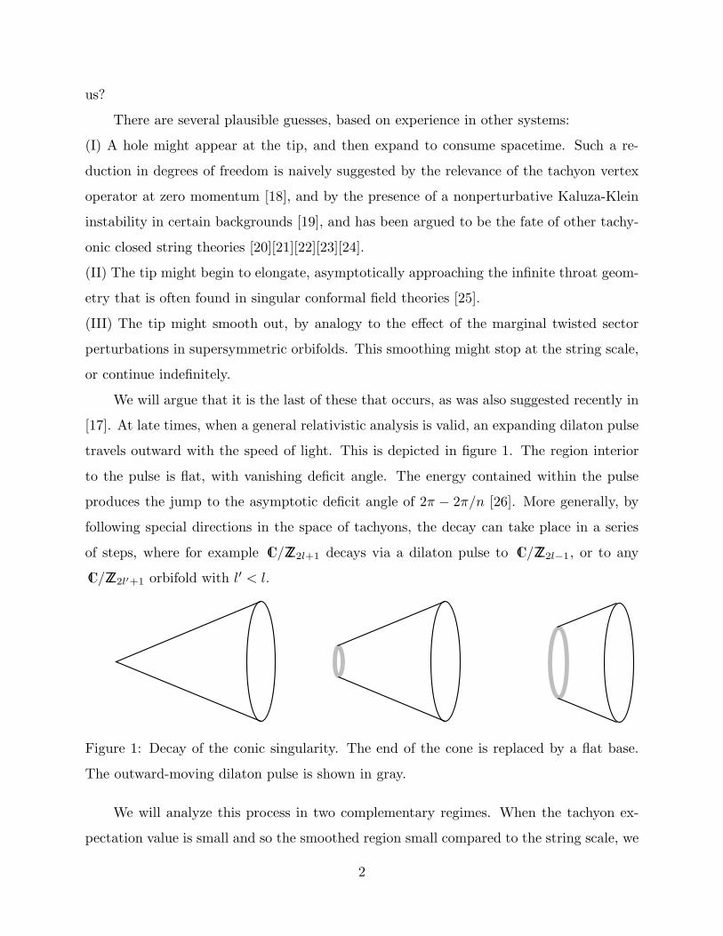
travels outward with the speed of light. This is depicted in figure 1. The region interior

to the pulse is flat, with vanishing deficit angle. The energy contained within the pulse

produces the jump to the asymptotic deficit angle of 2π − 2π/n [26]. More generally, by

following special directions in the space of tachyons, the decay can take place in a series

of steps, where for example IC/ZZ2l+1 decays via a dilaton pulse to IC/ZZ2l−1, or to any

IC/ZZ2l′+1 orbifold with l′ < l.

Figure 1: Decay of the conic singularity. The end of the cone is replaced by a flat base.

The outward-moving dilaton pulse is shown in gray.

We will analyze this process in two complementary regimes. When the tachyon ex-

pectation value is small and so the smoothed region small compared to the string scale, we

2

use D-brane probes [27], whose world-volume theory is a quiver gauge theory [28]. This is

the substring regime. D-branes on supersymmetric orbifolds have been studied extensively;

we extend these techniques to study non-supersymmetric orbifold compactifications with

closed string tachyons. The probes see a smoothed geometry when the tachyon is nonzero.

When the smoothing region exceeds the string length scale, we can instead use a general

relativistic description, and we argue that the solution has the form in figure 1. This is the

gravity regime. Because of α′ corrections, we do not have a controlled approximation that

connects the two regimes, but we argue that together they give a simple and consistent

picture of a transition from a conic singularity to flat space via tachyon condensation.

These same complementary descriptions have been applied to type I instantons and to

supersymmetric ALE spaces [28].

If one or more of these singularities is part of a compact manifold, then the initial

stages of tachyon condensation will be the same near each orbifold fixed point, producing

a smooth compact geometry. Unlike the noncompact system, which evolves forever, we

will argue that the compact space collapses toward a Big Crunch in finite time.

If we put N D3-branes on the fixed plane, and consider the near horizon limit, then the

system is expected to be dual to a nonsupersymmetric gauge theory [29]. The fixed plane

is partly transverse to the D3-brane, and in the large-radius limit of the AdS5 × S5/ZZn

background we find a dramatic instability that grows toward the boundary of AdS. We

argue that at large ’t Hooft coupling these nonsupersymmetric field theories are unphysical.

This contrasts with the more benign infrared Coleman-Weinberg instabilities evident on

the field theory side at weak ’t Hooft coupling (small radius), which arise in theories whose

gravity duals have tachyons at large radius [16][30].

The analysis can also be applied to orbifolds the form ICq/Γ, where Γ is a discrete

subgroup of the rotation group that fixes a point in ICq. If Γ 6⊂ SU(q) then the background

does not preserve supersymmetry, and there are twisted-sector tachyons localized at the

fixed point. For q = 1 there is no Γ that preserves supersymmetry, but for q ≥ 2 there will

be.

We study several IC2/ZZn examples, where analysis of the quiver theories on D-brane

probes leads to predictions for transitions between different orbifolds. There is a new effect

3

that can occur in this case: we exhibit infinite sequences of examples with transitions from

nonsupersymmetric ALE spaces to supersymmetric ones. We again expect a gravitational

background for large tachyon VEV that involves an expanding shell of dilaton gradient,

combined with metric curvature. In this case the total energy of the transition region must

vanish, since both the initial and final ALE spaces have vanishing energy as measured by

the falloff of the gravitational fields at infinity. (We will explain why this is not inconsistent

with positive energy theorems.)

For large n in Γ = ZZn, an angular direction is small for a significant range of radii

and it is useful to go to a T -dual picture involving NS5-branes [31]. These transitions

therefore provide a closed string analogue of the open string brane descent relations [32],

in that we can realize for example any Ak space (and therefore the equivalent dual system

of k + 1 NS5-branes) via tachyon condensation (and/or marginal deformation) from a

non-supersymmetric ALE space. Also, by adding an R-R flux, which has little effect on

the geometry, we obtain a system which has a conjectured dual description in terms of

fluxbranes [33][34][23][24][35][36].

This realization of supersymmetric ALE spaces (and therefore NS branes) by closed-

string tachyon condensation is very reminiscent of similar constructions in open string

theory [10]. In this regard, we should emphasize that certain puzzles that arise in the open

string case arise here as well [17].2 In particular, in open string tachyon condensation, one

finds gauge fields without sufficient perturbative charged matter to Higgs them [37][38],

but open string field theory calculations at disk order suggest that they are nonetheless

lifted classically [10][39][40]. In the tachyonic closed string systems we study here, there are

twisted RR gauge potentials without perturbative charged matter; our evidence suggests

that the defect is nonetheless smoothed and the RR potential lifted. In both the open

and closed string cases, it would be very interesting to understand the classical stringy

effect, evidently going beyond ordinary effective quantum field theory, which allows gauge

fields to be so lifted. In the closed string case, it would be interesting to understand an

analogue of the quantum confinement effect identified in the open string case in [41]; here

2 We thank M. Berkooz, P. Kraus, E. Martinec, and other participants of the Amsterdam

Summer workshop for discussions on this.

4

as there one has D-branes charged under the gauge group of interest (in our case these are

the fractional D-branes, whose condensation might lead to confinement of twisted strings

into untwisted strings).

The organization of this paper is as follows. In §2 we discuss the IC/ZZn orbifold,

including the twisted sector spectrum and the quantum symmetry group of the orbifold

theory. We also discuss the difference between orbifolds and ALE spaces that do not

have orbifold descriptions. We consider D-brane probes in the orbifold theory, deriving

the quiver representation. In §3 we analyze the quiver theory/linear sigma model for the

IC/ZZn orbifolds and their twisted deformations, discussing both generic decays and de-

cays that leave lower-order orbifolds. In §4 we develop the general relativistic description

of these same solutions. We discuss renormalization group evolution and time evolution.

These are similar, in that both lead to a smoothed region that grows without bound, but

there are differences in the details. We discuss the consistency between the renormaliza-

tion group analysis and the c-theorem. We then discuss the fate of compact spaces with

nonsupersymmetric orbifold points, and the consequences of our results for AdS/CFT du-

ality. In §5, we analyze transitions in the IC2/Γ case by means of the quiver theories, and

exhibit decays from non-SUSY to SUSY ALE spaces. In the general relativistic regime

we explain how our results are consistent with positive energy theorems. Finally, in §6 we

discuss dual systems, including fluxbranes, and in §7 mention some directions for further

research.

2. The IC/ZZn Orbifold

2.1. Closed String Spectrum

Let us start by reviewing some of the basic properties of the IC/ZZn orbifold conformal

field theory [13][14][15]. These orbifolds are defined by identifying the 8-9 plane under a

rotation R through 2π/n. This allows two possible actions on the spinors,

R = exp(2πiJ89/n) or exp(2πiJ89) exp(2πiJ89/n) , (2.1)

where J89 is the rotation generator. For either choice, Rn acts trivially on spacetime

and so is either 1 or exp(2πiJ89) = (−1)F. If Rn = (−1)F, the orbifold group (which is

5

actually ZZ2n in this case) includes this operator and so projects out spacetime fermions

and introduces tachyons in the bulk. Because we want to have all tachyons localized at

the fixed point we must have Rn = 1. For the two choices (2.1) one finds

Rn = (−1)F or (−1)(n+1)F . (2.2)

Thus, only the second choice of R is acceptable, and only for n odd:

R = exp

(

2πin+ 1

nJ89

)

, n = 2l + 1 . (2.3)

In the sector twisted by Rk (1 ≤ k ≤ n − 1), in the light-cone Green-Schwarz de-

scription there are six real untwisted scalars, one complex scalar twisted by k/n, and four

complex fermions twisted by k/2+k/2n. The standard calculation of the zero-point energy

givesα′

4m2 =

−k/2n , k even ,

(k − n)/2n , k odd .(2.4)

Thus the lowest state is tachyonic in every twisted sector. There are also excited state

tachyons in many sectors. For example, when k = 1 the lowest twisted scalar excitation

takes (1 − n)/2n to (3 − n)/2n and so this state is tachyonic for n > 3. Our analysis will

be rather coarse, and so we will generally not distinguish the ground state in each sector

from excited states with the same symmetries.

We wish to ask, where do these tachyonic perturbations take the system? Since they

are in the twisted sectors, their initial effect is in the neighborhood of the fixed point.

There are two contexts to consider. First, we could add the tachyonic vertex operators

to the Hamiltonian. Tachyonic states correspond to relevant vertex operators, so they

change the IR behavior of the world-sheet theory. We are then interested in determining

the renormalization group (RG) flow. Second, we could consider a time-dependent string

solution that begins as a small but exponentially growing tachyonic perturbation of the

orbifold. We are then interested in the subsequent time evolution.

Physically these are distinct questions. The first is an off-shell question from the

point of view of string theory, but well posed as question in two-dimensional quantum field

theory. The second is an on-shell question in string theory. In fact we will find, as has

6

been seen in other contexts, that the scale and time evolutions are similar. In both cases

the question can be posed in the classical string limit, with no string loop effects. If the

world-sheet theory were to become singular, for example if the dilaton were to become

large, then this framework would break down, but we will find that at least generically

this does not happen.

The orbifold preserves an SO(7, 1) × U(1) subgroup of the parent SO(9, 1). In addi-

tion there is a new “quantum” symmetry that appears in the orbifolded theory [42]: the

twist is conserved, mod n.3 The lowest tachyons in general break the quantum symme-

try completely but leave the SO(7, 1) × U(1) unbroken (in the RG case) or break it to

SO(7) × U(1) (in the time-dependent case). In some cases we will consider perturbations

that leave part of the quantum symmetry unbroken, while in others we will find that a

new quantum symmetry, unrelated to the original one, emerges asymptotically.

Actually, the evolution is more restricted than would follow from spacetime symmetry

alone. The XM and ψM (of the RNS description) upon which the SO(7, 1) or SO(7)

acts do not appear in the perturbation. These fields therefore remain free, whereas the

symmetry would allow a warp factor depending on the other coordinates.

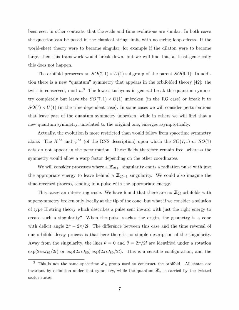
We will consider processes where a ZZ2l+1 singularity emits a radiation pulse with just

the appropriate energy to leave behind a ZZ2l−1 singularity. We could also imagine the

time-reversed process, sending in a pulse with the appropriate energy.

This raises an interesting issue. We have found that there are no ZZ2l orbifolds with

supersymmetry broken only locally at the tip of the cone, but what if we consider a solution

of type II string theory which describes a pulse sent inward with just the right energy to

create such a singularity? When the pulse reaches the origin, the geometry is a cone

with deficit angle 2π − 2π/2l. The difference between this case and the time reversal of

our orbifold decay process is that here there is no simple description of the singularity.

Away from the singularity, the lines θ = 0 and θ = 2π/2l are identified under a rotation

exp(2πiJ89/2l) or exp(2πiJ89) exp(2πiJ89/2l). This is a sensible configuration, and the

3 This is not the same spacetime ZZn group used to construct the orbifold. All states are

invariant by definition under that symmetry, while the quantum ZZn is carried by the twisted

sector states.

7

dynamical process allows one to reach it. However, on the 2l-fold covering space, the lines

θ = 0 and θ = 2π are identified under the action of (−1)F, and so there is a branch cut

in the spinor fields. This is the essential difference from the orbifold: in the orbifold the

untwisted fields are single-valued on the covering space. We could similarly consider a

wedge of any opening angle θo, where the plane is generically not a covering space. Again,

dynamically we could construct a state that has this behavior away from the singularity,

but that within a string distance of the singularity has some complicated description, not

based on a free CFT, if the singularity is resolved at all. Indeed, we will find many example

of orbifolds decaying to such spaces; we will use the terms ‘quasi-orbifold’ or ‘quasi-ALE

(QALE)’ to refer to these more general spaces that are locally Euclidean but are not

obtained as orbifolds of a single-valued theory on Euclidean space.

2.2. Open String Spectrum

We now consider a Dp-brane probe of the geometry. Here as in many other contexts,

D-brane probes [28] and closely related linear sigma model techniques [43] are useful for

obtaining a broader view of the space of closed string backgrounds than is available from

perturbation theory about a specific world-sheet CFT. In studying a D-brane probe, the low

energy quantum field theory on its world-volume is only valid in the substring regime, where

the VEVs of world-volume scalars (scaled to have dimensions of length) are sufficiently

small compared to the string length√α′. We will also study the D-brane probes in

the classical limit, and in doing so will self-consistently find results consistent with the

string coupling remaining bounded throughout the tachyon decay process. It would be an

interesting, but distinct, question to relax the gs → 0 limit we consider here and analyze

the quantum dynamics on D-brane probes in these backgrounds, a question that could be

considered both before and after the tachyons condense.

The classical world-volume theories of D-branes probing orbifold singularities were

worked out in a beautiful paper by Douglas and Moore [28]. The orbifold group Γ has

both a geometric action R and an action γR on the Chan-Paton indices,

|ψ, i, j〉 → γR ii′ |Rψ, i′, j′〉γ−1R j′j . (2.5)

8

For branes that are free to move away from the orbifold singularity, there must be a

distinct image for each element of Γ and so the Chan-Paton indices transform in the regular

representation. These branes have integer tensions and charges. Irregular representations

correspond to fractional branes bound to the fixed locus. We will be interested in the

regular case; as we have noted in the introduction, fractional branes are confined once the

singularity is resolved, but the full mechanism is not understood.

We will consider a Dp-brane probe that is extended in the directions µ = 0, 1, . . . , p and

localized in the directions m = p+1, . . . , 7 and in the orbifolded 8-9 plane. The treatment

will be uniform for the IIA or IIB theories, and for all p in the respective theories. We take

a single copy of the regular representation, but the discussion readily extends to N copies.

For Γ = ZZn, R cyclically permutes the D-brane images and so γR jk = δj+1,k. The indices

j, k are understood to be defined mod n, so in particular γR n1 = 1. It is more convenient

to work in a basis in which the spacetime action is not so evident but the spectrum and

its quiver representation are simple:

γR jk = e2πij/nδjk . (2.6)

The low energy theory is itself an “orbifold” of the N = 4 world-volume theory of a

D-brane in flat space, obtained by projecting out gauge theory fields that are not invariant

under the action (2.5). The massless open string fields are the vector potential Aµjk, the

collective coordinates Xmjk and Zjk = (X8 + iX9)jk, and the spinor ξjk in the 8 of SO(7, 1)

and with J89 = +12 . The real and imaginary parts of ξ form the 16 of SO(9, 1); we will

suppress the SO(7, 1) spinor index. The orbifold projection (2.5) on the operation (2.3),

(2.6) retains fields with j − k + (n+ 1)J89 = 0. The surviving fields are then

Aµ jj , Xmjj , Zj,j+1 , ξj,j−l , (2.7)

where j runs from 1 to n = 2l + 1 and indices are defined mod n. The conjugates are

Zj+1,j and ξj,j+l.

Thus the gauge group is U(1)n, with the collective coordinate Zj,j+1 having charge

+1 under U(1)j and charge −1 under U(1)j+1, while ξj,j−l has charge +1 under U(1)j

and charge −1 under U(1)j−l. The spectrum can be succinctly expressed through “quiver”

9

diagrams [28]. For each factor in the product gauge group, the diagram has a node; for

Γ = ZZn these are in one-to-one correspondence with the range of the Chan-Paton indices.

A field with charge +1 under U(1)j and charge −1 under U(1)k is denoted by an arrow

from node k to node j. For more general representations of Γ the gauge group is a product∏

j U(Nj) and the arrows represent bifundamentals. Arrows beginning and ending on the

same node are adjoints, which of course are neutral in the case of U(1)n. For the example

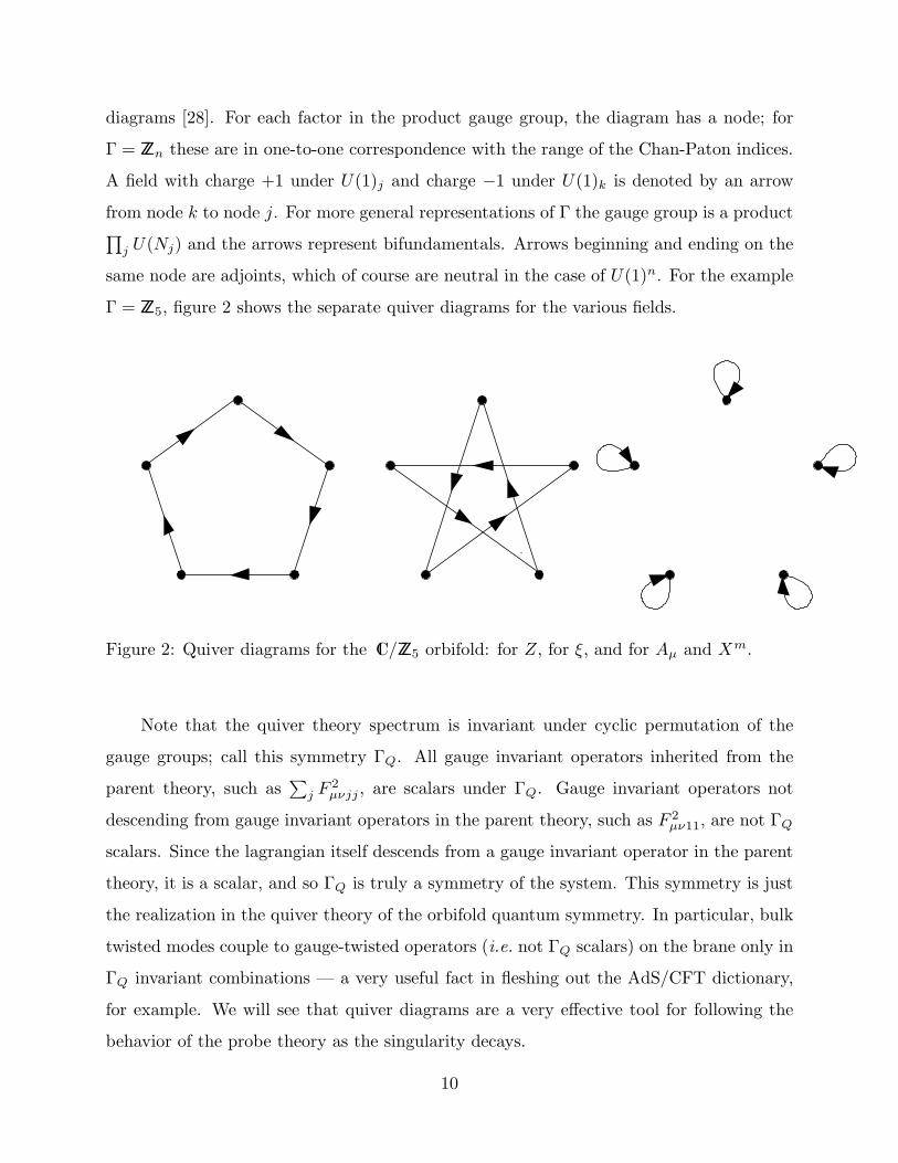
Γ = ZZ5, figure 2 shows the separate quiver diagrams for the various fields.

Figure 2: Quiver diagrams for the IC/ZZ5 orbifold: for Z, for ξ, and for Aµ and Xm.

Note that the quiver theory spectrum is invariant under cyclic permutation of the

gauge groups; call this symmetry ΓQ. All gauge invariant operators inherited from the

parent theory, such as∑

j F2µνjj , are scalars under ΓQ. Gauge invariant operators not

descending from gauge invariant operators in the parent theory, such as F 2µν11, are not ΓQ

scalars. Since the lagrangian itself descends from a gauge invariant operator in the parent

theory, it is a scalar, and so ΓQ is truly a symmetry of the system. This symmetry is just

the realization in the quiver theory of the orbifold quantum symmetry. In particular, bulk

twisted modes couple to gauge-twisted operators (i.e. not ΓQ scalars) on the brane only in

ΓQ invariant combinations — a very useful fact in fleshing out the AdS/CFT dictionary,

for example. We will see that quiver diagrams are a very effective tool for following the

behavior of the probe theory as the singularity decays.

10

The potential for the scalars is classically, at the orbifold point,

V =1

2

∑

j,m

(Xmjj −Xm

j+1,j+1)2|Zj,j+1|2 +

1

2

∑

j

(

|Zj,j+1|2 − |Zj−1,j|2)2

, (2.8)

where the overall normalization will not be important. We are interested in the Higgs

branch, where Xmjj is independent of j and the Zj,j+1 are nonzero. This corresponds to

a D-brane probe of the orbifold geometry. On the Coulomb branch the Xmjj depend on

j and the Zj,j+1 vanish. This branch corresponds to the probe separating into fractional

D-branes trapped at the singularity, and it disappears in the deformed geometry. On the

Higgs branch there is a Yukawa interaction

LY =∑

j

ξj,j−lξj−l,j+1Zj+1,j . (2.9)

Note that each interaction forms a closed loop on the quiver diagram.

We now consider the geometry of the Higgs branch. The vanishing of the potential

(2.8) implies that the magnitude |Zj,j+1| is independent of j. Of the n U(1) symmetries,

the diagonal decouples. The remaining n − 1 gauge symmetries can be used to set the

phases of the Zj,j+1 equal as well, so that the common value Zj,j+1 = Z parameterizes

the branch. The branch is thus two-dimensional, as it should be for the interpretation of

a probe. The gauge choice leaves unfixed a ZZn gauge symmetry, whose generator is

exp

(

−2πi

n

∑

j

jQj

)

. (2.10)

This identifies Z → e2πi/nZ, so the probe moduli space is indeed the IC/ZZn spacetime.

For each of the fields (2.7) there is one massless mode, where the field is independent of j.

This is the correct spectrum for a D-brane probe.

The moduli space metric, as measured by the probe kinetic term, is obtained by

integrating out the higgsed gauge fields. In a general gauge, the potential requires that on

the moduli space Zj,j+1 = reiθj . The kinetic terms are then

Lk =n

∑

j=1

∣

∣

∣(∂µ + iAµ jj − iAµ j+1,j+1)Zj,j+1

∣

∣

∣

2

=

n∑

j=1

[

(∂r)2 + r2(∂µθj −Bµj)2]

.

(2.11)

11

We have defined the relative gauge potentials, Bµj = Aµ jj − Aµ j+1,j+1, which tauto-

logically satisfy the constraint∑

Bµj = 0. The total U(1) is unbroken and decouples.

Integrating out the broken gauge fields subject to the constraint gives

Bµj = ∂µ(θj − θ) , θ =1

n

n∑

k=1

θk . (2.12)

Inserting this into the kinetic term gives the manifestly gauge invariant result

Lk = n[

(∂r)2 + r2(∂θ)2]

. (2.13)

As deduced above, the periodicity of θ is 2π/n. Rescaling to θ = nθ, with canonical period

2π, the kinetic term becomes

Lk = n (∂r)2 +r2

n(∂θ)2 , (2.14)

corresponding to the metric of a flat ZZn cone,

ds2 = n dr2 +r2

ndθ2 , (2.15)

as expected. For future reference note that we can define θ as

θ = arg(Zn1Z12 . . . Zn−1,n) ; (2.16)

the RHS is gauge invariant, so the period of θ is manifestly 2π.

The gauge bosons that have been integrated out have masses of order r/α′, while

excited string states with masses of order α′−1/2 have been ignored. The result is therefore

valid in the substringy regime [27], r ≪ α′1/2. We have also ignored quantum corrections

in the world-volume theory. This is valid because the world-volume fluctuations are open

string fields, and we have taken gs → 0 at the beginning — we have posed the problem in

classical string theory.

There is a closely related context in which world-volume quantum corrections would

be important. The world-volume theory of the D1-brane provides a linear sigma model

construction analogous to those in [43] of the F-string orbifold CFT [44]. In this one must

let the quantum world-volume theory flow to the IR fixed point. In the present case we

know independently, from the orbifold construction, that the fixed point action is the free

action (2.13).

12

3. Decay of IC/ZZn in the Substring Regime

3.1. Generic Tachyon VEVs: Breaking the Quantum Symmetry

In the initial stage of the instability, the tachyon VEV is small and so the geometry

is modified only in the substringy region near the tip of the cone. D-brane probes are

therefore the effective tool for investigating the geometry. The closed string background

determines the low energy quantum field theory on the probe. This can be obtained

directly from a calculation of the disk amplitude with a tachyon vertex operator plus open

string vertex operators, as in the appendix of ref. [28]. For our purposes, however, it will

suffice to identify the world-volume theory by matching with the quantum numbers of the

closed string tachyons.

¿From the discussion in §2.1, the tachyons generically break the quantum symmetry

completely, so this will be broken in the world-volume theory. We are in the substringy

regime, so we are interested in the leading effects in powers of Z. In the potential, this

would be a mass term

∆V =

n∑

j=1

m2j |Zj,j+1|2 . (3.1)

A term of definite quantum charge k would have a coefficient proportional to e2πijk/n.

Since there are tachyons with all charges except for the untwisted k = 0, one obtains

arbitrary masses subject to the constraint∑

j m2j = 0. It is then useful to reexpress the

mass term as

∆V = −n

∑

j=1

λj

(

|Zj,j+1|2 − |Zj−1,j|2)

,

n∑

j=1

λj = 0 . (3.2)

The notation is suggested by the supersymmetric case, where λj would be the Fayet-

Iliopoulos (FI) coefficient for U(1)j.

On the moduli space we now have

|Zj,j+1|2 − |Zj−1,j |2 = λj . (3.3)

For generic λj the Zj,j+1 are therefore distinct, and one of these has magnitude less than

the rest, say Z12. When this vanishes the remaining n − 1 Zj,j+1 are still nonzero. It

follows that U(1)n is broken to U(1) everywhere on the moduli space, and so there is no

13

orbifold point. The moduli space is smoothed; topologically it is IR2. The gauge-invariant

combination Zn1Z12 . . .Zn−1,n, which now vanishes linearly when Z12 → 0, is a good

coordinate.

We can confirm these conclusions by finding the probe metric. Define ρj iteratively,

ρ2j = ρ2

j−1 + λj , ρ1 = 0 . (3.4)

Then with Zj,j+1 = rjeiθj , eq. (3.3) implies

r2j = r2 + ρ2j , r ≡ r1 . (3.5)

The kinetic term is now

Lk =n

∑

j=1

[

(∂rj)2 + r2j (∂µθj −Bµj)

2]

. (3.6)

Enforcing the constraint∑

j Bµj = 0 with a Lagrange multiplier λµ, the equation of motion

for Bµj is r2j (∂µθj−Bµj) = λµ. Inserting this into the constraint determines the multiplier,

λµ

n∑

j=1

1

r2j= ∂µθ , (3.7)

where θ =∑

j θj is defined as in eq. (2.16) and so has period 2π. The action then takes

the simple form

Lk = n(r)(∂r)2 +r2

n(r)(∂θ)2 , (3.8)

where

n(r) =n

∑

j=1

r2

r2 + ρ2j

. (3.9)

The corresponding metric is

n(r)dr2 +r2

n(r)dθ2 ; (3.10)

for constant n(r) this is the metric (2.15)of a cone cone of deficit angle 2π/n. The function

n(r) interpolates smoothly from n(0) = 1 (the term j = 1) to n(∞) = n. Thus the

metric (3.10) is nonsingular at the origin and connects smoothly onto the original IC/ZZn

geometry asymptotically, as in figure 3.

14

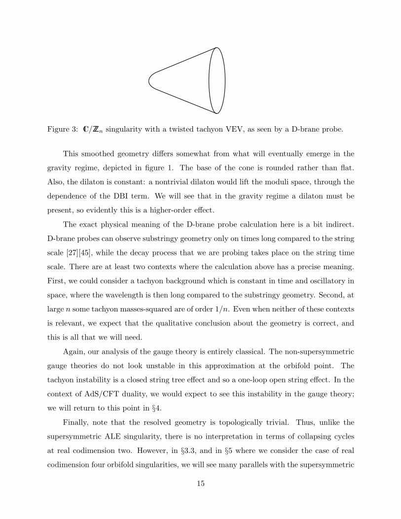
Figure 3: IC/ZZn singularity with a twisted tachyon VEV, as seen by a D-brane probe.

This smoothed geometry differs somewhat from what will eventually emerge in the

gravity regime, depicted in figure 1. The base of the cone is rounded rather than flat.

Also, the dilaton is constant: a nontrivial dilaton would lift the moduli space, through the

dependence of the DBI term. We will see that in the gravity regime a dilaton must be

present, so evidently this is a higher-order effect.

The exact physical meaning of the D-brane probe calculation here is a bit indirect.

D-brane probes can observe substringy geometry only on times long compared to the string

scale [27][45], while the decay process that we are probing takes place on the string time

scale. There are at least two contexts where the calculation above has a precise meaning.

First, we could consider a tachyon background which is constant in time and oscillatory in

space, where the wavelength is then long compared to the substringy geometry. Second, at

large n some tachyon masses-squared are of order 1/n. Even when neither of these contexts

is relevant, we expect that the qualitative conclusion about the geometry is correct, and

this is all that we will need.

Again, our analysis of the gauge theory is entirely classical. The non-supersymmetric

gauge theories do not look unstable in this approximation at the orbifold point. The

tachyon instability is a closed string tree effect and so a one-loop open string effect. In the

context of AdS/CFT duality, we would expect to see this instability in the gauge theory;

we will return to this point in §4.

Finally, note that the resolved geometry is topologically trivial. Thus, unlike the

supersymmetric ALE singularity, there is no interpretation in terms of collapsing cycles

at real codimension two. However, in §3.3, and in §5 where we consider the case of real

codimension four orbifold singularities, we will see many parallels with the supersymmetric

15

case.

3.2. World-sheet Linear Sigma Model

As we noted above, the D1-brane gauge theory provides the starting point for a LSM

representation of the F-string world-sheet theory. Let us digress slightly to explain the

picture of the tachyon decay process which emerges from this point of view.

The LSM description involves considering a simple gauge theory in the UV which flows

to the world-sheet CFT of interest in the IR [43]. In the context of quiver theories on D1-

branes at orbifold points, the classical moduli space is the orbifold space (as we reviewed

in §2.2), which is the target space for the F-string world-sheet CFT. Based on this and

the discrete symmetries of the theory arising for appropriate choice of theta angles, it was

argued in [44] that the D1-brane quiver theory provides a linear sigma model formulation

of the orbifold CFT, with the caveat that without supersymmetry one must fine-tune away

the quantum potential on the moduli space in order to reach the orbifold CFT in the IR

(which then enjoys an accidental supersymmetry).

We are interested in the effect on the world-sheet CFT when the tachyon VEVs are

turned on in spacetime, which means in terms of a renormalization group analysis that

a relevant operator is added to the world-sheet CFT action (taking the tachyons at zero

spacetime momentum). We would like to describe this deformation from the UV LSM

quiver theory. As we have discussed, the tachyons transform under the quantum symmetry

in the IR CFT, and this symmetry exists already in the UV quiver theory. Therefore we

can identify twisted operators in the UV theory which will generically mix with the twisted-

sector tachyon vertex operators in the IR. The twisted couplings of interest include the λj

in (3.2) above. These are the most relevant twisted deformations in the UV, and we will

focus on their effects.

The RG flow diagram of this theory appears as in the following figure.

16

OrbifoldCFT

1/e 2

λv

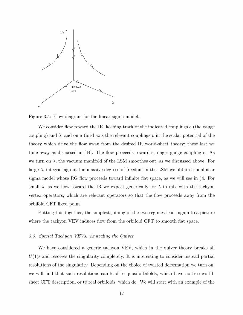
Figure 3.5: Flow diagram for the linear sigma model.

We consider flow toward the IR, keeping track of the indicated couplings e (the gauge

coupling) and λ, and on a third axis the relevant couplings v in the scalar potential of the

theory which drive the flow away from the desired IR world-sheet theory; these last we

tune away as discussed in [44]. The flow proceeds toward stronger gauge coupling e. As

we turn on λ, the vacuum manifold of the LSM smoothes out, as we discussed above. For

large λ, integrating out the massive degrees of freedom in the LSM we obtain a nonlinear

sigma model whose RG flow proceeds toward infinite flat space, as we will see in §4. For

small λ, as we flow toward the IR we expect generically for λ to mix with the tachyon

vertex operators, which are relevant operators so that the flow proceeds away from the

orbifold CFT fixed point.

Putting this together, the simplest joining of the two regimes leads again to a picture

where the tachyon VEV induces flow from the orbifold CFT to smooth flat space.

3.3. Special Tachyon VEVs: Annealing the Quiver

We have considered a generic tachyon VEV, which in the quiver theory breaks all

U(1)s and resolves the singularity completely. It is interesting to consider instead partial

resolutions of the singularity. Depending on the choice of twisted deformation we turn on,

we will find that such resolutions can lead to quasi-orbifolds, which have no free world-

sheet CFT description, or to real orbifolds, which do. We will start with an example of the

17

former case and then proceed to the transitions between real orbifolds that are our main

interest.

Consider for example the case that λ1 = −λ2 > 0, for which eq. (3.3) implies that one

bifundamental is greater than the rest,

|Z12|2 = |Zj,j+1|2 + λ1 , j 6= 1 . (3.11)

The maximum unbroken gauge symmetry is now U(1)n−1, where all Zj,j+1 other than Z12

vanish, so we expect that the symmetry is partially resolved to ZZn−1.

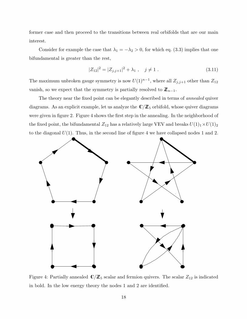
The theory near the fixed point can be elegantly described in terms of annealed quiver

diagrams. As an explicit example, let us analyze the IC/ZZ5 orbifold, whose quiver diagrams

were given in figure 2. Figure 4 shows the first step in the annealing. In the neighborhood of

the fixed point, the bifundamental Z12 has a relatively large VEV and breaks U(1)1×U(1)2

to the diagonal U(1). Thus, in the second line of figure 4 we have collapsed nodes 1 and 2.

Figure 4: Partially annealed IC/ZZ5 scalar and fermion quivers. The scalar Z12 is indicated

in bold. In the low energy theory the nodes 1 and 2 are identified.

18

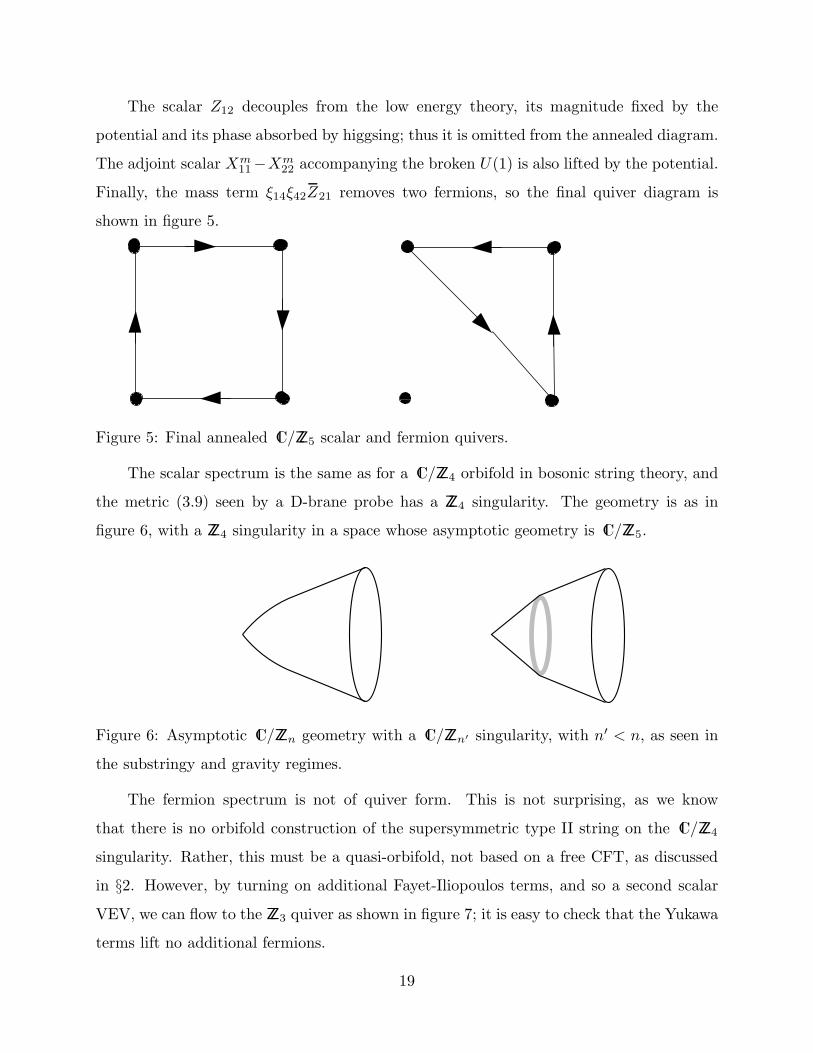
The scalar Z12 decouples from the low energy theory, its magnitude fixed by the

potential and its phase absorbed by higgsing; thus it is omitted from the annealed diagram.

The adjoint scalar Xm11−Xm

22 accompanying the broken U(1) is also lifted by the potential.

Finally, the mass term ξ14ξ42Z21 removes two fermions, so the final quiver diagram is

shown in figure 5.

Figure 5: Final annealed IC/ZZ5 scalar and fermion quivers.

The scalar spectrum is the same as for a IC/ZZ4 orbifold in bosonic string theory, and

the metric (3.9) seen by a D-brane probe has a ZZ4 singularity. The geometry is as in

figure 6, with a ZZ4 singularity in a space whose asymptotic geometry is IC/ZZ5.

Figure 6: Asymptotic IC/ZZn geometry with a IC/ZZn′ singularity, with n′ < n, as seen in

the substringy and gravity regimes.

The fermion spectrum is not of quiver form. This is not surprising, as we know

that there is no orbifold construction of the supersymmetric type II string on the IC/ZZ4

singularity. Rather, this must be a quasi-orbifold, not based on a free CFT, as discussed

in §2. However, by turning on additional Fayet-Iliopoulos terms, and so a second scalar

VEV, we can flow to the ZZ3 quiver as shown in figure 7; it is easy to check that the Yukawa

terms lift no additional fermions.

19

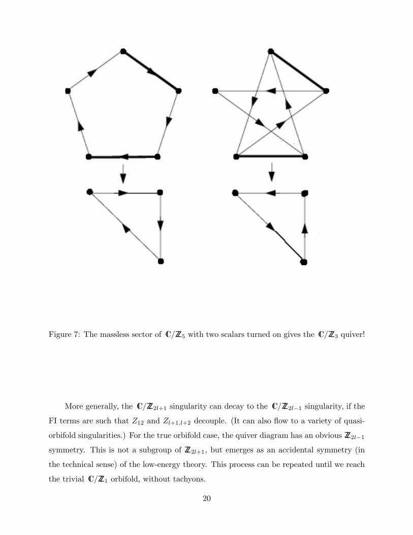
Figure 7: The massless sector of IC/ZZ5 with two scalars turned on gives the IC/ZZ3 quiver!

More generally, the IC/ZZ2l+1 singularity can decay to the IC/ZZ2l−1 singularity, if the

FI terms are such that Z12 and Zl+1,l+2 decouple. (It can also flow to a variety of quasi-

orbifold singularities.) For the true orbifold case, the quiver diagram has an obvious ZZ2l−1

symmetry. This is not a subgroup of ZZ2l+1, but emerges as an accidental symmetry (in

the technical sense) of the low-energy theory. This process can be repeated until we reach

the trivial IC/ZZ1 orbifold, without tachyons.

20

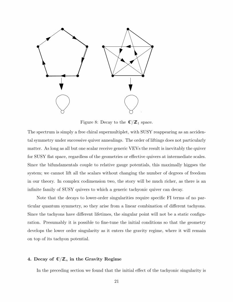
Figure 8: Decay to the IC/ZZ1 space.

The spectrum is simply a free chiral supermultiplet, with SUSY reappearing as an acciden-

tal symmetry under successive quiver annealings. The order of liftings does not particularly

matter. As long as all but one scalar receive generic VEVs the result is inevitably the quiver

for SUSY flat space, regardless of the geometries or effective quivers at intermediate scales.

Since the bifundamentals couple to relative gauge potentials, this maximally higgses the

system; we cannot lift all the scalars without changing the number of degrees of freedom

in our theory. In complex codimension two, the story will be much richer, as there is an

infinite family of SUSY quivers to which a generic tachyonic quiver can decay.

Note that the decays to lower-order singularities require specific FI terms of no par-

ticular quantum symmetry, so they arise from a linear combination of different tachyons.

Since the tachyons have different lifetimes, the singular point will not be a static configu-

ration. Presumably it is possible to fine-tune the initial conditions so that the geometry

develops the lower order singularity as it enters the gravity regime, where it will remain

on top of its tachyon potential.

4. Decay of IC/ZZn in the Gravity Regime

In the preceding section we found that the initial effect of the tachyonic singularity is

21

to smooth the geometry. As with any tachyon, an essential question is the nature of the

final state: does the tachyon potential have a minimum, or does the instability continue

without end? The D-brane probe analysis in the previous section breaks down when the

size of the smoothed region reaches the string scale. We do not have tools to probe this

regime, so will study the question by going beyond it to the regime of small curvature.

If we were to find that the RG flow in that regime carries us back to higher curvature,

this would indicate the presence of a minimum with curvature of order the string scale. In

fact, we will find that the flow goes toward ever-smaller curvature.4 Thus the geometry

evolves forever, generating an arbitrarily large region of arbitrarily small curvature, which

contains a lower-order singularity if the initial state has been appropriately fine-tuned.

4.1. RG Flow

We now study the RG flow of the world-sheet NLSM corresponding to a background

of the massless closed string fields. Owing to discrete symmetries, we need only consider

the metric and dilaton. Note that there is no explicit tachyon field in this regime. The

instability, whose initial stage is represented by a tachyon in the orbifold description, would

now be a property of the solutions to the low energy field equations. The RG equations

areGMN = −β[GMN ] + ∇MξN + ∇NξM ,

Φ = −β[Φ] + ξM∇MΦ ,(4.1)

where GMN is the string metric, a dot denotes the logarithmic derivative with respect to

world-sheet length scale ℓ∂ℓ, and

β[GMN ] = α′RMN + 2α′∇M∇NΦ ,

β[Φ] = α′(∇Φ)2 − α′

2∇2Φ .

(4.2)

The vector field ξM is arbitrary and represents the freedom to make a spacetime coordinate

change with the change of world-sheet scale. A convenient choice is ξM = α′∇MΦ, so that

GMN = −α′RMN , Φ =α′

2∇2Φ . (4.3)

4 We cannot exclude the possibility of a fixed point with curvature of order the string scale, but

the fact that both the substring and gravity geometries evolve toward smaller curvature strongly

suggest that this flow continues smoothly through the stringy regime.

22

In these coordinates the flow of the metric does not depend on the dilaton; this is possible

because the dilaton does not appear in the flat world-sheet action.

The perturbation leaves a (7 + 1)-dimensional free field theory, so the problem is

essentially two dimensional. It is convenient to work in conformal gauge, because the flow

(4.3) preserves that gauge. Thus,

ds2 = e2ω(dρ2 + ρ2dθ2) , (4.4)

where for generality we consider an arbitrary periodicity 0 ≤ θ ≤ 2π/ν. In this gauge, the

metric (2.15) for a cone of opening angle 2π/n corresponds to

ω =

(

ν

n− 1

)

ln ρ+ constant . (4.5)

In conformal gauge the RG is

ω =α′

2e−2ω∇2ω , (4.6)

where ∇2 is the Laplacian for the flat metric dρ2 + ρ2dθ2, which is ∂2ρ + ρ−1∂ρ for a

cylindrically symmetric solution.

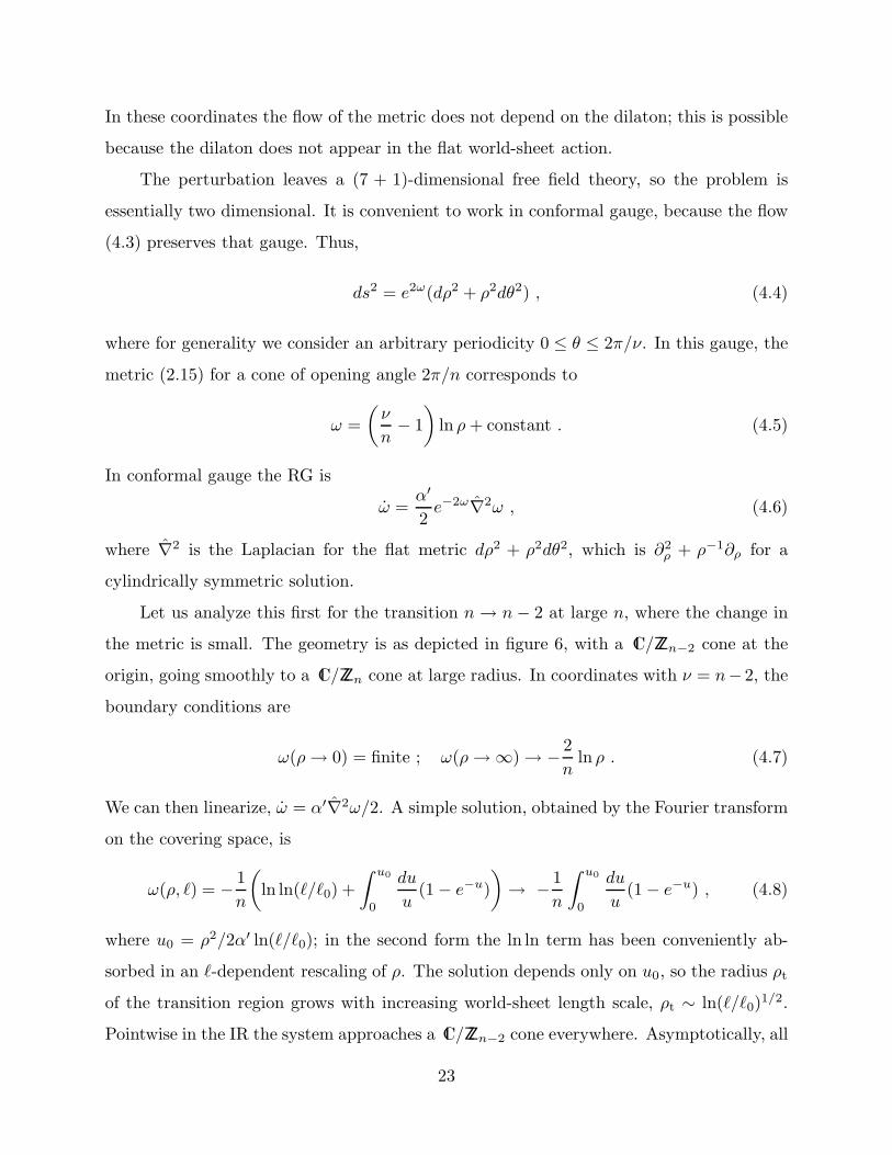
Let us analyze this first for the transition n → n− 2 at large n, where the change in

the metric is small. The geometry is as depicted in figure 6, with a IC/ZZn−2 cone at the

origin, going smoothly to a IC/ZZn cone at large radius. In coordinates with ν = n− 2, the

boundary conditions are

ω(ρ→ 0) = finite ; ω(ρ→ ∞) → − 2

nln ρ . (4.7)

We can then linearize, ω = α′∇2ω/2. A simple solution, obtained by the Fourier transform

on the covering space, is

ω(ρ, ℓ) = − 1

n

(

ln ln(ℓ/ℓ0) +

∫ u0

0

du

u(1 − e−u)

)

→ − 1

n

∫ u0

0

du

u(1 − e−u) , (4.8)

where u0 = ρ2/2α′ ln(ℓ/ℓ0); in the second form the ln ln term has been conveniently ab-

sorbed in an ℓ-dependent rescaling of ρ. The solution depends only on u0, so the radius ρt

of the transition region grows with increasing world-sheet length scale, ρt ∼ ln(ℓ/ℓ0)1/2.

Pointwise in the IR the system approaches a IC/ZZn−2 cone everywhere. Asymptotically, all

23

solutions to the diffusion equation with the given boundary conditions will have the same

form. The dilaton satisfies a diffusion equation as well and any initial dilaton gradient will

similarly diffuse outward.

For the full nonlinear evolution (4.6) we do not have a simple analytic result, but

given the diffusive nature of the equation we expect that in general the smoothed area

depicted in figure 3 grows without bound. Hence our conclusion that the flow found in the

substring region, toward smaller curvature, continues indefinitely in the gravity region.

There are two reasons that one might doubt this result. The first is the Zamolodchikov

c-theorem, showing irreversibility of the flow of the central charge [46]. Here we start with

an orbifold CFT of canonical central charge (15 in all for the type II string). In the IR, we

claim that the theory flows pointwise to flat spacetime, again with canonical central charge.

The reason that this is consistent is that the noncompactness of the target space invalidates

the c-theorem [47]. There are other cases of CFT theorems that are invalid in noncompact

target spaces. The classic example is the holomorphicity of conserved currents, which does

not hold for the world-sheet currents associated with rotational invariance in noncompact

directions [48]. For the c-theorem, the basic objects are the vacuum expectation values of

operator products. The string world-sheet vacuum fills out the entire target manifold, a

familiar IR effect, so the region of curvature makes a contribution of measure zero.

A second reason that one might have expected the opposite result is the example of

compact spaces of positive curvature, which flow to greater curvature. We claim that the

difference of boundary conditions in the compact and noncompact cases accounts for the

differing behaviors. In fact, there is a simple monotonicity result that makes this clear.

From the differential equation (4.3) it follows that

ℓ∂ℓ

∫

d2x√G = −α

′

2

∫

d2x√GR . (4.9)

For a manifold of spherical topology, the RHS is −4πα′ and so the volume is monotonically

decreasing. The curvature must at some point become stringy, and the low energy theory

break down. For the noncompact manifold the integral is not defined, but one can consider

the integral interior to a circle of some given radius (over a region such as depicted in

figure 3). The smoothing of the singularity does have the effect of reducing this volume,

24

whereas flow back toward a singular cone would increase the volume in contradiction to

the flow (4.9).

Finally, we might also be interested in the case that the original singularity is part of

a compact space. Most simply, consider T 2/ZZ3, which is a flat space of spherical topology,

with three IC/ZZ3 singularities each of deficit angle 4π/3. From the c-theorem, or from

eq. (4.9), one concludes that the space eventually flows to large curvature. The three

singularities begin to smooth, until the smoothed regions merge to form a rough sphere,

which then evolves toward smaller radius.

4.2. Dynamical Evolution

We now consider on-shell evolution,

β[GMN ] = β[Φ] = 0 , (4.10)

with the same β-functions (4.2). This is now a three-dimensional problem, since the

solution depends on time. It is convenient to work in the Einstein frame, where this

system is just a massless scalar canonically coupled to the metric. The initial metric is

again assumed to interpolate from IC/ZZn at infinity to IC/ZZn′ at the origin, with n′ < n.

This is true in both the Einstein and the string frames, because we assume that the dilaton

is nonsingular at the origin, while it goes to a constant at infinity (where the evolution has

not yet reached).

We do not have analytic solutions for this problem, but it is easy to deduce the general

form of the solutions. The constraint equations require that the change in deficit angle

be accompanied by energy density of matter. Since we can solve the equations with the

NS three-form field strength set to zero, so that the only matter involved is the massless

dilaton, this energy must be dilaton gradient and kinetic energy. This dilaton field will

radiate outward at the speed of light, as in figure 1. The time scale of the initial decay,

before the gravity regime, is the string scale, so this sets the initial width of the dilaton

pulse and the kink in the geometry, which then gradually broadens due to dispersion. For

n′ = n−2 at large n, an analytic treatment is again simple. The dilaton satisfies a massless

wave equation in flat spacetime, and the backreaction on the metric is a perturbative effect.

25

As a check, let us look for static solutions in the gravity regime, which would have

corresponded to minima of the tachyon potential that are visible in this regime. We will

take the most general form with SO(7, 1) × SO(2) spacetime symmetry:

ds2 = e2σ(r)ηµνdxµdxν + e2f(r)(dr2 + r2dθ2) . (4.11)

This is slightly more general than elsewhere, in that we allow the (7, 1) directions to be

warped; note also a slight change of notation, µ, ν = 0, . . . , 7. The dilaton field equation is

Φ′′

Φ′− 2Φ′ = −1

r− 8σ′ ⇒ (e−2Φ)′ =

c1re−8σ (4.12)

with integration parameter c1. The µν curvature equation reads

(rσ′)′

rσ′+ 8σ′ = 2Φ′ ⇒ e2Φ = c2rσ

′e8σ (4.13)

with integration parameter c2. Putting these together gives Φ′ = −c1c2σ′/2, and so

eΦ ∝ (ln r/r0)−c1c2/2(8+c1c2) , eσ ∝ (ln r/r0)

1/(8+c1c2) . (4.14)

These are doubly unacceptable: they do not go over to the unperturbed behavior at large

r, and they have a singularity at finite r = r0. Only the flat cone, the exceptional solution

with Φ and σ constant, survives.

It is interesting again to consider the T 2/ZZ3 orbifold, with nonsupersymmetric singu-

larities in a compact space. We cannot follow the behavior analytically, but might expect

that after the dilaton pulses have begun to cross the compact space, the time-averaged be-

havior will be that of a positively curved radiation dominated spacetime. Thus, it will reach

a Big Crunch in finite time, beyond which we cannot follow the evolution. One supposition

would be that the compact dimensions effectively disappear, leaving an eight-dimensional

noncritical string theory [18]. However, the simplest background in that theory — the

linear dilaton — has the wrong symmetries to be the endstate of our evolution, as the

dilaton gradient is spacelike.

4.3. Application to AdS/CFT

In ref. [29] it was argued that orbifolding should commute with AdS/CFT duality, so

that the dual of the orbifolded gauge theory is IIB string theory on the orbifolded spacetime.

26

This expectation is based on the fact that a duality like the AdS/CFT correspondence

concerns a single system with two dual descriptions; if orbifolding makes sense on one side

of the duality then the procedure can be mapped to the equivalent dual description of the

system given a complete duality dictionary translating between them. In the absence of

supersymmetry, if the orbifolding procedure produces a consistent physical system, this

requires any instabilities that arise to match up between the two equivalent descriptions.

The leading instability that arises in a string background is that of interest here, namely the

tachyons. In freely-acting orbifolds on the sphere component of the AdSp × Sq geometry,

the spectrum is classically tachyon-free. Non-freely acting orbifolds on the Sq do have

tachyons, and this has been considered at small ’t Hooft parameter [16], where the gauge

theory is perturbative. Now let us consider the situation at large ’t Hooft parameter, where

the AdS description is good.

The AdS description starts with N coincident D3-branes extended in the 0123 di-

rections. The orbifold produces a (7+1)-dimensional fixed plane. This plane contains

the D3-branes and extends in four transverse directions. The AdS curvature is small

on the string scale and so locally on the fixed plane the initial instability is the same

as in flat spacetime. In particular, the decay will release a given energy per unit

volume of the fixed plane, as measured in a local inertial frame. The invariant vol-

ume element is (r/RAdS)3d3x (r/RAdS)

−4r3dr, where x coordinatizes the field theory

dimensions and r is a coordinate along the radial direction of AdS5 × S5, with metric

(r/RAdS)2dx2 +(r/RAdS)

−2(dr2 + r2dΩ2). The translation to the global conserved energy

brings in an additional factor of r/RAdS, so the total energy released per unit gauge theory

volume is simply∫ ∞

0

dr r3 ∼ Λ4 . (4.15)

That is, it diverges quarticly in the gauge theory.

We can make a simple model of how this divergence might arise in the gauge theory.

Consider a state a U(1) gauge theory where we add a + and a − charge in a volume of

linear size ℓ. The kinetic energy is of order 2ℓ−1, but this is reduced somewhat by the

gauge theory potential, for a net 2 −O(g2)ℓ−1. Extrapolation would suggest a possible

instability at large g2 (to be precise, this theory will have a Landau pole in the UV, so we

27

must imagine a cutoff). In a globally supersymmetric theory, positivity of the energy is

guaranteed and so this instability is absent; thus, supersymmetric field theories can make

sense at large coupling. However, for nonsupersymmetric theories there is no guarantee

that they make sense at strong coupling. Indeed the result (4.15) suggests an instability of

just this sort: in a conformal theory we can produce pairs on any scale ℓ, and the integral

over all scales produces a quarticly divergent result. Note that this is much more severe

than the instabilities normally encountered in field theories (such as symmetry breaking),

which are IR effects and release a finite energy per unit volume. It is difficult to see how

this instability could have any sensible final state.

Indeed, the AdS picture is similarly pathological. We can quantitatively study the

large-n case ZZn → ZZn−2, because the dilaton essentially satisfies a free wave equation on

the AdS5 × S5 covering space,

R2AdS

r2∂2

t Φ =r2

R2AdS

∂2⊥Φ . (4.16)

The orbifold breaks the SO(6) symmetry of S5 so the dilaton is a superposition of different

angular states. For angular momentum L,

∂2⊥ = ∂2

r +5

r∂r −

L(L+ 4)

r2. (4.17)

Imagine that the decay starts everywhere at once at t = 0. This condition is conformally

invariant so the dilaton is a function only of rt. The wave equation (4.16) then becomes

an ordinary differential equation for ΦL(rt), and rt = R2AdS is a singular point. From the

dominant terms near the singular point one finds that

ΦL ∼ (R2AdS − rt)−3/2 (4.18)

for every partial wave L. Thus, the energy density diverges at finite time for any r; this

occurs when a geodesic from (r, t) = (∞, 0) reaches a given radius, carrying the information

about the divergent energy release at large radius.

Again, this instability is a property of large ’t Hooft parameter, and is not inconsistent

with the much milder instability found at small ’t Hooft parameter in ref. [16]. Note that

28

we have assumed that the ’t Hooft parameter does not run, as holds at large N . If the full

β function were in fact asymptotically free, then the theory would be stable in the UV,

and the instability that we are discussing would set in only below some scale. In this event

it is possible that there would be a stable final state.

5. IC2/ZZn Orbifolds and Non-SUSY to SUSY Flows

5.1. Orbifolds and Quivers

One of the interesting results of the study of open string tachyons has been the pos-

sibility of realizing stable branes, in particular SUSY branes, by open string tachyon con-

densation [10][32]. In this section, we study closed string tachyon condensation on IC2/ZZn

orbifolds by generalizing the D-brane probe approach of §3 to this case. We will exhibit

various transitions from non-supersymmetric, tachyonic IC2/ZZn orbifolds to supersymmet-

ric ALE spaces, and provide an infinite sequence of such flows which allows us to realize any

SUSY ALE space via closed-string tachyon condensation (or more generally a combination

of marginal deformation and tachyon condensation).

The discussion will parallel the IC/ZZn case. All the orbifolds that we consider will be

based on a twist of the form

R = exp

2πi

n(J67 + kJ89)

, (5.1)

depending on two integers n and k (mod 2n). We will denote the group generated by R

as ZZn(k). On spinors with J67 and J89 charge s67 = s89 = ±12, R acts as e±2πi(k+1)/2n.

On spinors with −s67 = s89 = ±12 it acts as e±2πi(k−1)/2n. The condition that Rn = 1 on

spinors forces k to be odd. If k is ±1, then R leaves half of the D = 10 spinors invariant

and so produces the familiar supersymmetric An−1 orbifold (for reviews see [49][50]). For

other values of k, at least some of the twisted sector ground states are tachyonic. If

2n is divisible by k + 1 or by k − 1, then R2n/(k+1) or R2n/(k−1) leaves some spinors

invariant. The associated twisted sector ground state is massless, and indeed is the same

as the corresponding twisted sector state in the supersymmetric orbifold (but note that

the respective cases k + 1 = 2 and k − 1 = 2 are trivial).

29

Let us now consider a D-brane probe in this background. Define

Z1 = X6 + iX7 , Z2 = X8 + iX9 . (5.2)

For the world-volume spinor in the 16 of SO(9, 1), its component with (s67, s89) =

(−12 ,−1

2) will be denoted χ and it component with (s67, s89) = (−12 ,+

12 ) will be de-

noted η (the remaining two components are the conjugates). The SO(5, 1) spinor indices,

respectively 4 and 4′, are suppressed. Using the techniques discussed in [28] and §2, one

finds the world-volume theory to be a U(1)n quiver theory with matter content

Aµ jj , Xmjj , Z1

j,j+1 , Z2j,j+k , χj,j−q−1 , ηj,j+q (k ≡ 2q + 1) . (5.3)

The classical scalar potential is

V = Tr

1

2[Z1, Z1]2 +

1

2[Z2, Z2]2 +

∣

∣[Z1, Z2]∣

∣

2+

∣

∣[Z1, Z2]∣

∣

2

. (5.4)

Using the Jacobi identity this can also be rewritten

V = Tr

1

2

(

[Z1, Z1] − [Z2, Z2])2

+ 2∣

∣[Z1, Z2]∣

∣

2

= Tr

1

2

(

[Z1, Z1] + [Z2, Z2])2

+ 2∣

∣[Z1, Z2]∣

∣

2

.

(5.5)

The Yukawa terms are

LY = Tr

[Z1, χ] η + [Z2, χ] η + h.c.

. (5.6)

5.2. The Example ZZ2l(2l−1): Non-SUSY ZZ2l to SUSY ZZ2

Now we analyze the case k = n−1, where n = 2l must be even because k is odd. Here

R = exp2πiJ89 exp2πi(J67 − J89)/2l (5.7)

is the same as in the supersymmetric case except for a factor of exp2πiJ89 = (−1)F,

which breaks supersymmetry. Note however that the special case l = 1, the IC2/ZZ2(1)

orbifold, is supersymmetric: R = exp2πi(J67 + J89)/2 leaves invariant spinors such that

s67 = −s89.

30

Before exciting tachyons, the geometry is the same as for the supersymmetric orbifold.

In particular, on the probe moduli space the condition that V vanish gives

Z1j,j+1 = Z1 , Z2

j+1,j = Z2 (independent of j) (5.8)

up to gauge transformation. Thus the probe has two complex moduli, as it should. The

origin, where the U(1)2l gauge symmetry is restored, is a ZZ2l singularity as in §2.2.

Before discussing the generic decay, it is interesting to consider first deformations

that preserve a ZZ2 ⊂ ZZ2l quantum symmetry. This ZZ2 acts on the lth twisted sector as

(−1)l, so only states twisted by powers of R2 can have VEVs. Since R2 = exp2πi(J67 −J89)/l, these sectors are exactly the same as for the supersymmetric IC2/ZZl(−1) orbifold.

In particular, there are no tachyons, so we are actually considering marginal deformations.

The perturbation of the gauge theory is then a supersymmetric D-term

∆V = −2l

∑

j=1

λjDj , Dj = |Z1j,j+1|2 − |Z2

j+1,j |2 − |Z1j−1,j|2 + |Z2

j,j−1|2 , (5.9)

where the sign of each term is determined by the U(1)j charge (note that for a k = −1

orbifold Z1 and Z2 are in chiral superfields, while for k = +1 it would be Z1 and Z2).

An overall additive constant is ignored. As in §2.2,∑2l

j=1 λj = 0, while the ZZ2 quantum

symmetry requires that λj = λj+l. Now consider the deformed moduli space; focus on the

second of forms (5.5) and note that the first term there is just∑2l

j=1D2j . The vanishing of

the second term requires that

Z1j,j+1Z

2j+1,j ≡ α (5.10)

be independent of j. Minimizing the D-terms then sets Dj = λj , which determines all of

the magnitudes in terms of |Z112| and α. Finally, the phases can be gauged away except

for∑2l

j=1 argZ1j,j+1, giving four real moduli in all.

There are still singularities. Consider the subspace α = 0. The condition Dj = λj

determines

|Z1j,j+1|2 − |Z2

j+1,j|2 = ρj + x , (5.11)

where ρj = ρj−1 + λj and x is undetermined. When x = −ρj0 for some j0, both Z1j0,j0+1

and Z2j0+1,j0

vanish. Further, the ZZ2 quantum symmetry implies that Z1j0+l,j0+l+1 and

31

Z2j0+l+1,j0+l vanish as well. There are then two unbroken U(1)’s, namely

∑j0+lj=j0+1Qj and

∑j0j=j0+l+1Qj , where Qj is the U(1)j charge and j is defined mod 2l. Thus, these l points

of restored gauge symmetry, which are generically distinct, are ZZ2 singularities on the

moduli space.

Thus far the discussion is the same as for the resolution of a supersymmetric

IC2/ZZ2l(−1) singularity while preserving a ZZ2 quantum symmetry: the result there would

be a ZZ2(−1) orbifold of a smooth ZZl ALE space. The difference for us is that the final

orbifold operation here contains an extra factor of (−1)F, so it must be ZZ2(1). Naively

one might expect this orbifold point to be nonsupersymmetric, but the discussion at the

beginning of this subsection shows that it is supersymmetric with the opposite supersym-

metry from that respected by R2. One can think of the final picture as follows: we resolve

the IC2/ZZl(−1) orbifold generated by R2 into a smooth ALE space preserving half of the

supersymmetry, and then make a ZZ2(1) orbifold which locally would preserve the other

half. In other words, we have a space of SU(2)1 ⊂ SO(4) = SU(2)1 × SU(2)2 holonomy,

with l orbifold singularities whose holonomy is in SU(2)2. The space as a whole has no

supersymmetry, but half of the supersymmetry survives in the smooth region and the other

half locally at the orbifold points. In the limit that the marginal deformation is taken to

infinity, we simply have a supersymmetric IC2/ZZ2(1) space, without tachyons.

We can verify this by examining the quivers. At the orbifold point, the potential

for the vanishing fields Z1j0,j0+1, Z

2j0+1,j0

, Z1j0+l,j0+l+1 and Z2

j0+l+1,j0+l is quartic so they

are massless, while all other scalars are massed up. One unbroken U(1) acts on indices

j = j0, j0 + l + 1, and the other on indices j = j0 + 1, j0 + l. Expanding the Yukawa

coupling (5.6) in components, one finds that ηj0+1,j0+l and ηj0+l+1,j0 do not appear in

terms with scalar expectation values, so these remain massless (note that these are neutral

under the unbroken U(1)’s). There must therefore also be two massless linear combina-

tions of χ’s; these come in the bifundamental representation of the unbroken U(1)2. The

correlation between U(1) charges and SO(5, 1) quantum numbers is the same as for the

IC/ZZ2(1) orbifold, namely the spectrum (5.3) at k = 1 with η in the adjoint and χ in the

bifundamental representation of the gauge group.

We now turn to the generic twisted state background. The full D-brane probe analysis

32

is less useful here, for two reasons. The first is that without any connection to supersym-

metry, the quantum symmetry alone does not fix the form of the quadratic mass terms

(specifically, the ratio of Z1 and Z2 masses); it requires the calculation of a disk ampli-

tude, as in the appendix to ref. [28]. More critically, for general mass terms allowed by the

quantum symmetry, there is no probe moduli space. This is not a problem — from the

spacetime point of view it is the same effect that a dilaton background would have — but

it makes it difficult to give a geometric interpretation in the substring regime.

Fortunately, we can largely deduce the fate of the instability by expanding around

the deformation already considered. Let us first deform IC2/ZZ2l(2l−1) along directions

that preserve the ZZ2 quantum symmetry as above, so as to have an orbifold of SU(2)2

holonomy in a space of SU(2)1 holonomy. The orbifold locally is supersymmetric and so

has marginal deformations in the twisted sector. These correspond to blowing the orbifold

points up into smooth ZZ2 ALE spaces of SU(2)2 holonomy. Thus we have small patches

of SU(2)2 holonomy in a larger region of SU(2)1 holonomy. This is only an approximate

solution to the equations of motion, and will in time evolve to a space of generic holonomy

and expand indefinitely as in the IC/ZZn case.

Note that the second blowing-up will not be exactly marginal, as the coupling to the

SU(2) curvature will break supersymmetry and presumably drive the marginal direction to

be tachyonic. If the extent of initial blowing-up is reduced, so as to condense the two steps

towards one, the ZZ2(1) twisted state will become more tachyonic, so we seem to connect

smoothly onto the original string-scale tachyon.

There is a seeming paradox here, whose resolution provides an elegant check on our

picture. The initial IC2/ZZ2l(2l−1) orbifold is an exact CFT, and so its tree-level energy (as

measured by the 1/r2 falloff of the metric) is zero. There is a tree-level tachyon, and so

the final state should have negative energy when the kinetic energy of the outgoing pulse

is subtracted.5 Does this not violate a positive energy theorem? In fact, there is no such

theorem: negative energy configurations of asymptotic ALE geometry exist [51].6 There is

5 This paradox did not arise for IC/ZZn, because in two dimensions a conic deficit angle is an

ADM energy.6 We would like to thank G. Horowitz for informing us about these spaces and explaining their

33

a negative energy theorem for any geometry that admits spinor fields going to a constant

at infinity [53][54]. The geometries of ref. [51] admit spinors, so it must be that any smooth

spinor field is antiperiodic under the asymptotic ALE identification. This is precisely the

geometry of the ZZ2l(2l−1) orbifold.

In the above example and the others we will consider in this section, we have studied in

detail the substring regime using D-brane probes, and in the case of marginal deformations,

we have also studied the regime far away from the original orbifold point using inheritance

from a related SUSY orbifold. Once tachyons turn on and the system evolves into the

gravity regime, we have not analyzed the subsequent GR solutions as explicitly as in the

IC/ZZn case. However, the following indicates that the behavior is as before. Consider a

configuration of negative energy. If the size of the configuration is scaled up by a factor λ,

the energy scales as λ2 (λ4 from the volume and λ−2 from the derivatives). This implies

that the potential is unbounded below in this direction.

5.3. The Example IC2/ZZ2l(3): Non-SUSY ZZ2l to SUSY ZZl

These results have a resemblance to phenomena that have been observed in open string

systems. The existence of a tachyon, which disappears as one goes along a marginal direc-

tion, is the same as in a D-brane/anti-D-brane system, where the string-scale tachyon at

small separation goes over to a long-range attraction as the branes are separated. The de-

cay of a nonsupersymmetric configuration to a supersymmetric configuration plus outgoing

radiation is also familiar.

There are many other similar flow patterns that can be deduced by studying the quiver

theories as we have done for the above case. One interesting sequence is for n = 2l and

k = 3,

R = exp

2πi

2l(J67 + 3J89)

, (5.12)

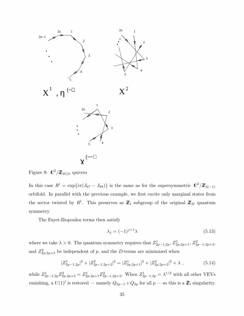
whose quiver diagrams are shown in figure 9.

significance, as well as sharing insights from his investigations into GR solutions for the IC2/ZZn

cases [52].

34

2n1

2

3

45

.

χ(−−)

..

1

2

3

4

5

2n

2n−1

X , η (−+)

2n 1

2

3

45

X1 2

......

Figure 9: IC2/ZZ2l(3) quivers

In this case Rl = expiπ(J67 − J89) is the same as for the supersymmetric IC2/ZZ2(−1)

orbifold. In parallel with the previous example, we first excite only marginal states from

the sector twisted by Rl. This preserves as ZZl subgroup of the original ZZ2l quantum

symmetry.

The Fayet-Iliopoulos terms then satisfy

λj = (−1)j+1λ (5.13)

where we take λ > 0. The quantum symmetry requires that Z12p−1,2p, Z

12p,2p+1, Z

22p−1,2p+2,

and Z22p,2p+3 be independent of p, and the D-terms are minimized when

|Z12p−1,2p|2 + |Z2

2p−1,2p+2|2 = |Z12p,2p+1|2 + |Z2

2p,2p+3|2 + λ , (5.14)

while Z12p−1,2pZ

22p,2p+3 = Z1

2p,2p+1Z22p−1,2p+2. When Z1

2p−1,2p = λ1/2 with all other VEVs

vanishing, a U(1)l is restored — namely Q2p−1 +Q2p for all p — so this is a ZZl singularity.

35

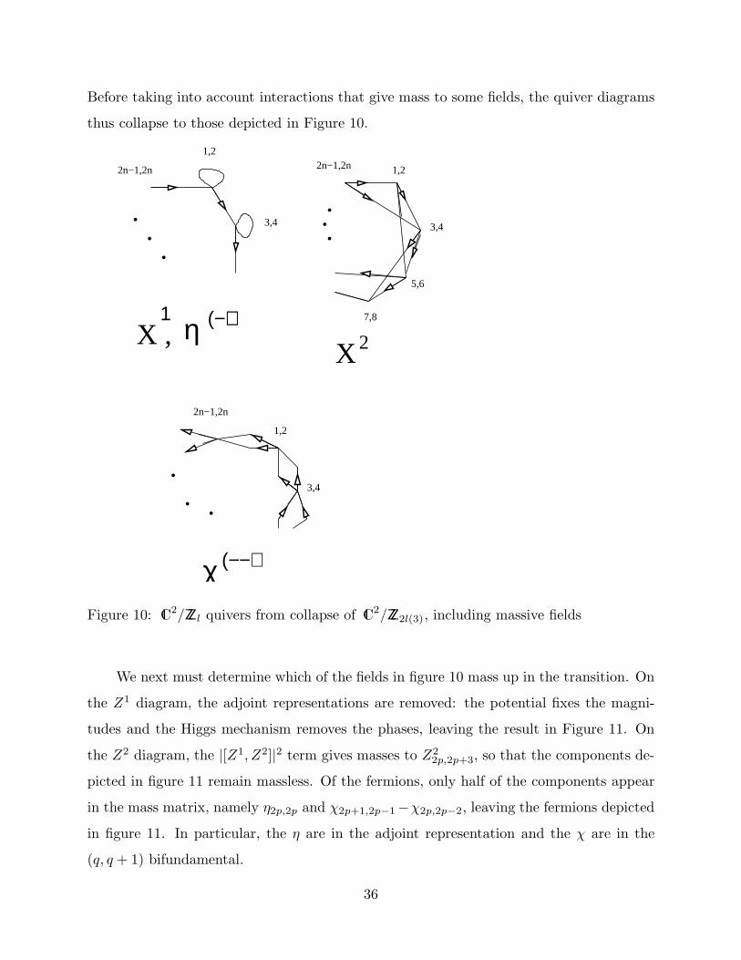
Before taking into account interactions that give mass to some fields, the quiver diagrams

thus collapse to those depicted in Figure 10.

X , η (−+)1

2n−1,2n

1,2

3,4

2n−1,2n 1,2

3,4

5,6

7,8

X 2

χ (−−)

2n−1,2n

1,2

3,4

...

...

.. .

Figure 10: IC2/ZZl quivers from collapse of IC2/ZZ2l(3), including massive fields

We next must determine which of the fields in figure 10 mass up in the transition. On

the Z1 diagram, the adjoint representations are removed: the potential fixes the magni-

tudes and the Higgs mechanism removes the phases, leaving the result in Figure 11. On

the Z2 diagram, the |[Z1, Z2]|2 term gives masses to Z22p,2p+3, so that the components de-

picted in figure 11 remain massless. Of the fermions, only half of the components appear

in the mass matrix, namely η2p,2p and χ2p+1,2p−1−χ2p,2p−2, leaving the fermions depicted

in figure 11. In particular, the η are in the adjoint representation and the χ are in the

(q, q + 1) bifundamental.

36

η (−+)(−−)

χ

2n−1,2n 1,2

5,6

3,4

1

2n−1,2n

1,2

3,4

2n−1,2n 1,2

3,4

5,6

7,8

X 2

1,2

3,4

5,6

2n−1, 2n

X

.

.

...

...

...

.

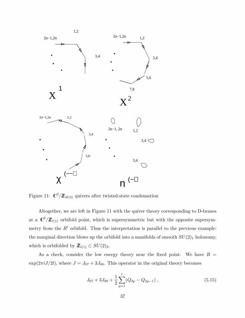
Figure 11: IC2/ZZ2l(3) quivers after twisted-state condensation

Altogether, we are left in Figure 11 with the quiver theory corresponding to D-branes

at a IC2/ZZl(1) orbifold point, which is supersymmetric but with the opposite supersym-

metry from the Rl orbifold. Thus the interpretation is parallel to the previous example:

the marginal direction blows up the orbifold into a manifolds of smooth SU(2)1 holonomy,

which is orbifolded by ZZl(1) ⊂ SU(2)2.

As a check, consider the low energy theory near the fixed point. We have R =

exp(2πiJ/2l), where J = J67 + 3J89. This operator in the original theory becomes

J67 + 3J89 +1

2

l∑

p=1

(Q2p −Q2p−1) , (5.15)

37

in the low energy theory, because this is the linear combination including the broken

generators that leaves the background invariant. This acts on the massless fields as

Z12p,2p+1 → 2Z1

2p,2p+1 , Z22p−1,2p+2 → 2Z2

2p−1,2p+2 (5.16)

and so it acts as J = 2(J67 + J89) in the low energy theory. The orbifold operation

exp(2πiJ/2l) is then ZZl(1) in the low energy theory.

There is another orbifold point, where Z22p−1,2p+2 = λ1/2 with all other VEVs van-

ishing. The analysis of the previous paragraph shows that this is a ZZl(−3), which is

nonsupersymmetric for l > 2.

In summary, we can obtain all supersymmetric ALE orbifolds by descent from non-

supersymmetric ones. The IC2/ZZ4(3) → IC2/ZZ2(1) flow is common to both this sequence

and the one discussed in §5.2.

5.4. The Example IC2/ZZ5(3) → IC/ZZ2(1): Tachyon Condensation

Since both of the above examples involved marginal as well as tachyonic deformations,

it is interesting to ask whether there are in fact examples where such transitions between

non-supersymmetric and supersymmetric ALE spaces proceed exclusively by tachyon con-

densation, without any marginal component. The following simple example exhibits this

possibility (which we expect to be generic). We will make the assumption that the twisted

deformations we turn on in the quiver world-volume QFT can be accessed by adjusting

modes in the tower of twisted states in the closed string sector. It would be interesting to

check this generic assumption more explicitly as in [28].

Start with the orbifold IC2/ZZ5(3). We can choose three independent λj such that

the D-terms induce VEVs for Z145, Z

151, and Z1

23. This preserves a U(1)2 subgroup of the

U(1)5 gauge symmetry, generated by combinations of charges Q4 +Q5 +Q1 and Q2 +Q3.

Plugging these VEVs into the component expansion of the interaction terms (5.5)(5.6)

as before, we find that the spectrum reduces to that of the IC/ZZ2(1) quiver theory, with

gauge group U(1)2, η in the adjoint and χ, Z1, and Z2 transforming as bifundamentals.

This theory does not have effectively supersymmetric subsectors, in contrast to those in

§5.2 and §5.3. So given our assumption about the availability of these deformations in the

38

closed string spectrum (including those that put the Lagrangian in supersymmetric form),

this provides an example of a truly tachyonic transition from a non-supersymmetric ALE

space to a supersymmetric one.

6. Dualities, Fluxbranes, and the Type 0 Tachyon

The results in the preceding sections describe transitions between different ALE spaces

(including flat space) by processes in which the string coupling remains bounded. While

this is sufficient for our purposes, it is also instructive to consider the predictions that these

results imply for processes in dual descriptions of the system. In particular we will consider

T -dual descriptions, in the angular direction, of the orbifolds that we have considered, as

well as the addition of R-R Wilson lines. The duals thus involve NS5-branes, fluxbranes,

and the type 0 tachyon.

6.1. IC/ZZn at Large n

An angular direction along which we rotate in performing a ZZn orbifold projection

ends up n times smaller than in the parent theory, so for n large it is of interest to T -dualize

along this direction in the region near the origin. Near but not at the origin, there is a

subspace that looks approximately like a cylinder, with twisted strings playing the role of

winding modes around the S1 direction of the cylinder:

Figure 12: The IC/ZZn cone at large n, with a twisted closed string.

In other words, there are many low-lying twisted states, which become Kaluza-Klein states

in the T -dual description. The formal T -dual of the cone metric (2.15) is

ds2 = ndr2 +nα′2

r2dθ2 . (6.1)

Also, the dilaton is now position-dependent,

eΦ = gs

√nα′

r. (6.2)

39

In the large-n limit the orbifold operation (2.3) is a small rotation times (−1)F, so on

the circle that we are T -dualing fields are twisted by (−1)F. Such a twist has three effects

on the T -dual description. First, the bulk theory is twisted by (−1)F, so it is the type 0

theory (type 0B if we began with IIA, and type 0A if we began with IIB). Second, in going

around the T -dual circle there is a twist by (−1)Q, where Q is the quantum symmetry dual

to the twist (−1)F. That is, type 0 fields that descend from the type II theory are periodic,

while type 0 fields that do not descend (including the type 0 tachyon) are antiperiodic.

Third, the periodicity of the dual coordinate is halved, 0 ≤ θ ≤ π.

The T -dual description is valid out to r ∼ n√α′, beyond which the T -dual circle is

small and the original circle is large. It also breaks down for r <√α′, where the curvature

becomes large. Thus, the apparent divergence of the dilaton (6.2) is irrelevant, as we

could have expected since the orbifold description is manifestly weakly coupled. We do

not have any good description in this region; it is some sort of effective ‘wall’ in spacetime,

whose properties can be deduced from the exact orbifold description. One property of

the wall that is not evident in the metric (6.1) is the breaking of translation invariance in

the θ-direction. The twisted modes of the orbifold transform under the finite ZZn quantum

symmetry rather than the infinite group ZZ characterizing true winding modes on a cylinder.

In the T -dual description, this means that the continuous translation symmetry along the

dual angular circle is broken to a discrete ZZn symmetry [55]. This suggests that the

wall is actually a line of n branes (defined broadly as defects which break translation

invariance) spaced equally along the T -dual circle. In the case of IC2/ZZn, this picture is

well understood, as we will review shortly, but for IC/ZZn we do not know of any suitable

candidate branes.

The twisted state tachyon of the original theory is just the bulk type 0 tachyon in

the T -dual description. The multiplicity of excited tachyons associated with the eight-

dimensional fixed plane on the orbifold side maps on the T -dual side to the multiplicity

of modes of the ten-dimensional type 0 tachyon. Because of the (−1)Q twist the decay

is most rapid at small r. The type 0 tachyon in ten dimensions has α′

4 m2 = −1

2 , and

the antiperiodic boundary condition should shift this upward by an amount of order the

40

inverse radius of the dual circle. Indeed, the most tachyonic mode has

α′

4m2 = −1

2+

1

2n(6.3)

For the partial resolution n→ n−2, it seems that the wall relaxes into a lower energy

state while a metric and dilaton perturbation (given by the T -dual of the picture in §4)

propagates outward. For the full decay n → 1, the tip of the cone and the associated

low-lying states disappear at the speed of light. In the T -dual picture, it seems that the

wall, where our control breaks down, is propagating to larger r at the speed of light. At

larger r, the angular direction gets smaller in this T-dual picture. It would be interesting

to try to extract from this a prediction for the type 0 tachyon, but this is not immediate

in our system here because the initial wall is present to act as a seed for the decay.

6.2. IC2/ZZn and NS5-Branes

For the orbifold IC2/ZZn at large n and fixed k, the angular direction generated by

J67 + kJ89 is again small and a T -dual picture is valid. This is best understood in the

supersymmetric cases k = ±1: the T -dual description has n evenly spaced NS5-branes

[31]. The sequences of transitions between non-supersymmetric and supersymmetric four-

dimensional ALE spaces detailed in §5 (and presumably many others like them) allow us to

produce any supersymmetric ALE space by closed-string tachyon condensation or marginal

deformation. Using the T -duality, we can restate this in terms of NS5-branes. Namely, any

number of NS5-branes can be obtained by condensation of modes in a non-supersymmetric

closed string background.

It is also interesting to look for a brane description of the tachyonic starting point.

In particular, in the case IC2/ZZ2l(2l−1) → IC2/ZZ2(1) one might have expected that since

the bosonic action is the same as in a supersymmetric IC2/ZZ2l orbifold, the T -duality

transformation would produce a similar configuration of 2l NS5-branes. However, the

factor (−1)F in the twist (5.7) modifies the T -duality as described in §6.1. The T -dual

circle is only half as large, so there are only l NS5-branes, while the bulk theory is type 0

theory with a (−1)Q twist around the T -dual circle. The marginal deformations that we

discussed descend from those of the supersymmetric ZZl theory, and so correspond to the

41

positions of the l NS5-branes. The tachyons, in the sectors of odd ZZ2 quantum symmetry,

are modes of the type 0 tachyon.

It would be interesting to pursue this type of dual description of the non-supersym-

metric ALE orbifolds further. It is straightforward to apply the general T -duality trans-

formation [56], but this results in a smeared 5-brane solution and we do not know the

localized form in general.

6.3. Adding RR Flux

A simple generalization is to add an RR Wilson line to the IC/ZZn orbifold,7 Cθ = 1

in coordinates where the identification is θ ∼ θ + 2π/n. The net phase is then 2π/n. In

M theory this corresponds to an orbifold by a 2π/n rotation accompanied by a shift by

1/n around the M theory circle. In a dual description where a linear combination of the

eleventh direction and the angular direction of the orbifold is taken to be the M direction,

this is a fluxbrane [33][34][23][24][35][36]. Because of the factor of (−1)F in the orbifold,

it is a fluxbrane in the type 0A theory [57] of strength BR2 = 1/n, or a fluxbrane in the

type IIA theory of strength BR2 = 1 + 1/n.

This duality is a strong-weak coupling duality, so that both sides are not simulta-

neously weakly coupled. However, on the fluxbrane side the coupling varies with radial

distance from the origin, becoming weaker toward the origin. If we fix the string coupling

to be gs < 1 on the orbifold side, on the fluxbrane side one has a region r < lsg1/3s n = nlP,11

near the origin which has string coupling g(f)s < 1. For large n and gs > 0, this region can

cover many string lengths. We will study the predictions of our results combined with the

conjectured orbifold/fluxbrane duality for decay of the Type 0A tachyon in this region.

In our analysis in the bulk of this paper, we worked in the classical string limit. As we

have just learned, in order to dualize to a fluxbrane side with a significant region of weak

coupling near the origin, we must relax this limit somewhat, and consider a nonvanishing

orbifold string coupling, though we can keep it weak. For the remainder of this section,

we will assume that the decay process we studied proceeds similarly at weak but nonzero

coupling.

7 We thank A. Strominger for discussions on this issue.

42

RR field strengths couple to extra powers of gs in the action and so for weak string

coupling they have only a small effect on the tachyon decay process we have studied. The

decay will proceed as we have described, with the RR flux ultimately dispersing when we

reach the flat space endpoint. For the partial decay n → n − 2, the outgoing pulse must

contain a negative RR flux 2π( 1n − 1

n−2 ). In the dual fluxbrane, the flux near the origin

increases in the transition, from 1n

to 1n−2

. According to the conjectured duality dictionary

in [23][24], this addition of flux takes the 0A theory closer to the flat space IIA theory.

Therefore, by assuming the dualities described in [23][24][35], and combining them

with our results on classical tachyon decay in orbifolds, we predict that the type 0A tachyon

in ten dimensions decays toward the flat ten-dimensional IIA vacuum. This agrees with

the conjecture for the fate of the Type 0A tachyon made in [24] based on extrapolating

to a regime where non-perturbative decays from 0A to IIA occur [19][58]. Our route to

this conclusion is somewhat more direct, as we use our classical results on tachyon decays

in orbifolds rather than non-perturbative instanton effects. However, these statements

are still predicated on the conjectural non-supersymmetric strong-weak coupling duality

[57][23] assumed in [24]. Therefore we regard this as a mild consistency check of the

proposal that the type 0A tachyon drives the theory to the type IIA vacuum.

7. Conclusions

In this paper we have exhibited strong evidence that tachyonic non-supersymmetric

ALE spaces decay to supersymmetric ALE spaces (including flat space). There are several

interesting lessons and directions for future work that emerge from our analysis.

On the theoretical side, as we have emphasized at various points, our results are rather

similar to ones that emerge in the study of open string tachyon condensation and its rela-

tion to unstable brane annihilation. It would be very interesting to understand how far the

analogy between twisted strings and open strings goes. Is there a notion of confinement of

twisted strings into ordinary untwisted closed strings? Is there a simplification of closed

string field theory if one focuses on twisted states and regards untwisted strings as deriva-

tive degrees of freedom obtained in internal legs of the diagrams? What does the similarity

43

between closed string and open string processes say about the extent of applicability of

K-theoretic techniques as a function of gs?

We should reemphasize, as discussed in the introduction, that there is a similar puz-

zling issue in the two cases. Namely as in the open string case, our results point to the need

for a strictly classical stringy mechanism, different from the Higgs mechanism, for lifting

gauge bosons living on decaying defects. It is perhaps a clue that the disappearance of

these gauge bosons and the other phenomena we have observed occurs in the closed string

as well as open string context: whatever the physics is that gives rise to these processes,

it is not tied uniquely to the open string perturbation expansion since it arises for twisted

closed strings as well.

Another related lesson is the existence of a large class of non-supersymmetric config-

urations which, while unstable, do not “decay to nothing”, as a class of non-SUSY models

without massless fermions are known to do [19][58][21]. Instead, they decay via a relatively

well-controlled weakly coupled process to stable supersymmetric configurations. It would

be very interesting to understand the fate of compact non-supersymmetric orbifolds of the

superstring with massless fermions, particularly since as we discussed the time-dependent

physics in the compact case is very similar to that of a cosmology heading toward a big

crunch singularity.

In terms of model-building, these results, while mostly negative for supersymmetry

breaking, at least may help direct attention to more stable possibilities than geometrical

orbifolds for breaking SUSY. The fact that the noncompact models decay to SUSY spaces

provides a new indication of the intrinsic role of SUSY within the theory. Again, the

question of the fate of compact examples which are most relevant for phenomenological

model-building is still open.

Finally, it would be interesting to extend these results to other cases, such as inter-

secting ALE spaces probed by different combinations of D-branes, and the type I theory.

In particular, dualities suggest that the case of singular ALE spaces intersecting at angles

introduces novel phenomena [59], and it will be interesting to see if our techniques in this

paper can provide insight into this case (or a deformation of it).

Noncompact tachyonic orbifolds of the heterotic string may have a similar fate to

44

those we discussed here, but in that case there are no D-brane probes available to study

the substring regime. The heterotic case will require an understanding of the dynamics of

the vector bundle formed by the gauge bosons as well as the configuration of dilaton and

metric. Under RG flow the cases with a standard embedding of the orbifold action into

the gauge group will behave as our models here; it would be interesting to study also the

time-dependent on-shell spacetime solutions in the heterotic string.

Acknowledgements

We would like to thank M. Rocek for many useful and enjoyable discussions on this

topic. We would also like to thank M. Berkooz, D. Gross, G. Horowitz, S. Kachru, P.

Kraus, E. Martinec, A. Strominger, and W. Taylor for very useful discussions. This work

was supported in part by the NSF under grant numbers PHY97-22022 and PHY99-07949.

A. A. and E.S. would like to thank the hospitality of the Institute for Theoretical Physics at

UCSB where this work was initiated. A.A. is also supported in part by an NSF Graduate

Fellowship, and A.A. and E.S. by the DOE (contract DE-AC03-76SF00515 and OJI) and

the Alfred P. Sloan Foundation.

45

References

[1] K. Bardakci, “Dual Models and Spontaneous Symmetry Breaking”, Nucl.Phys.

B68(1974)331; K.Bardakci and M.B.Halpern, “Explicit Spontaneous Breakdown in

a Dual Model”, Phys.Rev.D10 (1974)4230; K.Bardakci and M.B.Halpern, “Explicit

Spontaneous Breakdown in a Dual Model II: N Point Functions”, Nucl. Phys.

B96(1975)285; K.Bardakci, “Spontaneous Symmetry Breakdown in the Standard Dual

String Model”, Nucl.Phys.B133(1978)297.

[2] V. A. Kostelecky and S. Samuel, “On A Nonperturbative Vacuum For The Open

Bosonic String,” Nucl. Phys. B 336, 263 (1990);

[3] T. Banks and L. Susskind, “Brane - Antibrane Forces,” hep-th/9511194.

[4] A. Sen, “Non-BPS states and branes in string theory,” hep-th/9904207.

[5] J. A. Harvey, D. Kutasov and E. J. Martinec, cp “On the relevance of tachyons,”

hep-th/0003101.

[6] A. A. Gerasimov and S. L. Shatashvili, “On exact tachyon potential in open string

field theory,” JHEP 0010, 034 (2000) [hep-th/0009103].

[7] D. Kutasov, M. Marino and G. Moore, “Some exact results on tachyon condensation

in string field theory,” JHEP 0010, 045 (2000) [hep-th/0009148].

[8] D. J. Gross and W. Taylor, “Split string field theory. I,” JHEP 0108, 009 (2001)

[hep-th/0105059].

[9] L. Rastelli, A. Sen and B. Zwiebach, “Vacuum string field theory,” hep-th/0106010.

[10] Owing to a lack of written reviews, for reviews and further references we suggest

http://online.itp.ucsb.edu/online/mp01/sen1/ ,

http://www.slac.stanford.edu/spires/find/hep/www?rawcmd=ti+tachyon%23 .

[11] L. J. Dixon, J. A. Harvey, C. Vafa and E. Witten, “Strings On Orbifolds,” Nucl. Phys.

B 261, 678 (1985).

[12] L. J. Dixon, J. A. Harvey, C. Vafa and E. Witten, “Strings On Orbifolds. 2,” Nucl.

Phys. B 274, 285 (1986).

[13] A. Dabholkar, “Strings on a cone and black hole entropy,” Nucl. Phys. B 439, 650

(1995) [hep-th/9408098].

[14] A. Dabholkar, “Quantum corrections to black hole entropy in string theory,” Phys.

Lett. B 347, 222 (1995) [hep-th/9409158].

[15] D. A. Lowe and A. Strominger, “Strings near a Rindler or black hole horizon,” Phys.

Rev. D 51, 1793 (1995) [hep-th/9410215].

[16] A. Adams and E. Silverstein, “Closed string tachyons, AdS/CFT, and large N QCD,”

hep-th/0103220.

[17] E. J. Martinec and W. McElgin, “String theory on AdS orbifolds,” hep-th/0106171.

[18] S. P. de Alwis, J. Polchinski and R. Schimmrigk, “Heterotic Strings With Tree Level

Cosmological Constant,” Phys. Lett. B 218, 449 (1989).

46

[19] E. Witten, “Instability Of The Kaluza-Klein Vacuum,” Nucl. Phys. B 195, 481 (1982).

[20] S. Kachru, J. Kumar and E. Silverstein, “Orientifolds, RG flows, and closed string

tachyons,” Class. Quant. Grav. 17, 1139 (2000) [hep-th/9907038].

[21] M. Fabinger and P. Horava, “Casimir effect between world-branes in heterotic M-

theory,” Nucl. Phys. B 580, 243 (2000) [hep-th/0002073].

[22] G. T. Horowitz and L. Susskind, “Bosonic M theory,” hep-th/0012037.

[23] M. S. Costa and M. Gutperle, “The Kaluza-Klein Melvin solution in M-theory,” JHEP

0103, 027 (2001) [hep-th/0012072].

[24] M. Gutperle and A. Strominger, “Fluxbranes in string theory,” JHEP 0106, 035

(2001) [hep-th/0104136].

[25] E. Witten, “Some comments on string dynamics,” hep-th/9507121.

[26] S. Deser, R. Jackiw and G. ’t Hooft, “Three-Dimensional Einstein Gravity: Dynamics

Of Flat Space,” Annals Phys. 152, 220 (1984).

[27] M. R. Douglas, D. Kabat, P. Pouliot and S. H. Shenker, “D-branes and short distances

in string theory,” Nucl. Phys. B 485, 85 (1997) [hep-th/9608024].

[28] M. R. Douglas and G. Moore, “D-branes, Quivers, and ALE Instantons,” hep-

th/9603167.

[29] S. Kachru and E. Silverstein, “4d conformal theories and strings on orbifolds,” Phys.

Rev. Lett. 80, 4855 (1998) [hep-th/9802183].

[30] A. A. Tseytlin and K. Zarembo, “Effective potential in non-supersymmetric SU(N)

x SU(N) gauge theory and interactions of type 0 D3-branes,” Phys. Lett. B 457, 77

(1999) [hep-th/9902095].

[31] H. Ooguri and C. Vafa, “Two-Dimensional Black Hole and Singularities of CY Mani-

folds,” Nucl. Phys. B 463, 55 (1996) [hep-th/9511164].

[32] N. Berkovits, A. Sen and B. Zwiebach, “Tachyon condensation in superstring field

theory,” Nucl. Phys. B 587, 147 (2000) [hep-th/0002211].

[33] F. Dowker, J. P. Gauntlett, D. A. Kastor and J. Traschen, Phys. Rev. D 49, 2909

(1994) [hep-th/9309075].

[34] F. Dowker, J. P. Gauntlett, S. B. Giddings and G. T. Horowitz, Phys. Rev. D 50,

2662 (1994) [hep-th/9312172].

[35] M. S. Costa, C. A. Herdeiro and L. Cornalba, “Flux-branes and the dielectric effect

in string theory,” hep-th/0105023.

[36] P. M. Saffin, “Gravitating fluxbranes,” Phys. Rev. D 64, 024014 (2001) [gr-qc/0104014].

[37] M. Srednicki, “IIB or not IIB,” JHEP 9808, 005 (1998) [hep-th/9807138].

[38] E. Witten, “D-branes and K-theory,” JHEP 9812, 019 (1998) [hep-th/9810188].

[39] I. Ellwood and W. Taylor, “Open string field theory without open strings,” Phys.

Lett. B 512, 181 (2001) [hep-th/0103085].

[40] I. Ellwood, B. Feng, Y. He and N. Moeller, “The identity string field and the tachyon

vacuum,” JHEP 0107, 016 (2001) [hep-th/0105024].

47

[41] P. Yi, “Membranes from five-branes and fundamental strings from Dp branes,” Nucl.

Phys. B 550, 214 (1999) [hep-th/9901159].

[42] C. Vafa, “Quantum Symmetries Of String Vacua,” Mod. Phys. Lett. A 4, 1615 (1989).

[43] E. Witten, “Phases of N = 2 theories in two dimensions,” Nucl. Phys. B 403, 159

(1993) [hep-th/9301042].

[44] E. Silverstein and Y. S. Song, “On the critical behavior of D1-brane theories,” JHEP

0003, 029 (2000) [hep-th/9912244].

[45] M. Li and T. Yoneya, “D-particle dynamics and the space-time uncertainty relation,”

Phys. Rev. Lett. 78, 1219 (1997) [hep-th/9611072].

[46] A. B. Zamolodchikov, “Irreversibility Of The Flux Of The Renormalization Group In

A 2-D Field Theory,” JETP Lett. 43, 730 (1986) [Pisma Zh. Eksp. Teor. Fiz. 43, 565

(1986)].

[47] J. Polchinski, “Scale And Conformal Invariance In Quantum Field Theory,” Nucl.

Phys. B 303, 226 (1988).

[48] T. Banks and L. J. Dixon, “Constraints On String Vacua With Space-Time Super-

symmetry,” Nucl. Phys. B 307, 93 (1988).

[49] D. Anselmi, M. Billo, P. Fre, L. Girardello and A. Zaffaroni, “ALE manifolds and

conformal field theories,” Int. J. Mod. Phys. A 9, 3007 (1994) [hep-th/9304135].

[50] C. V. Johnson, “D-brane primer,” hep-th/0007170.

[51] C. LeBrun, “Counterexamples to the Generalized Positive Action Conjecture”, Comm.

Math. Phys. 118, 591 (1988).

[52] G. Horowitz, work in progress

[53] E. Witten, “A Simple Proof Of The Positive Energy Theorem,” Commun. Math. Phys.

80, 381 (1981).

[54] G. W. Gibbons and C. N. Pope, “Positive Action Theorems For Ale And Alf Spaces,”

ICTP-81-82-20.

[55] R. Gregory, J. A. Harvey and G. Moore, “Unwinding strings and T-duality of Kaluza-

Klein and H-monopoles,” Adv. Theor. Math. Phys. 1, 283 (1997) [hep-th/9708086].

[56] T. H. Buscher, “A Symmetry Of The String Background Field Equations,” Phys. Lett.

B 194, 59 (1987); “Path Integral Derivation Of Quantum Duality In Nonlinear Sigma

Models,” Phys. Lett. B 201, 466 (1988).

[57] O. Bergman and M. R. Gaberdiel, “Dualities of type 0 strings,” JHEP 9907, 022

(1999) [hep-th/9906055].

[58] F. Dowker, J. P. Gauntlett, G. W. Gibbons and G. T. Horowitz, “The Decay of mag-

netic fields in Kaluza-Klein theory,” Phys. Rev. D 52, 6929 (1995) [hep-th/9507143].

[59] A. Uranga, work in progress; K. Dasgupta, private communication.

48