arX

iv:h

ep-t

h/00

1112

7v2

18

Sep

2001

PUPT-1966

hep-th/0011127

The evolution of unstable black holes

in anti-de Sitter space

S. S. Gubser and I. Mitra

Joseph Henry Laboratories, Princeton University, Princeton, NJ 08544

Abstract

We examine the thermodynamic stability of large black holes in four-dimensional anti-

de Sitter space, and we demonstrate numerically that black holes which lack local

thermodynamic stability often also lack stability against small perturbations. This

shows that no-hair theorems do not apply in anti-de Sitter space. A heuristic argument,

based on thermodynamics only, suggests that if there are any violations of Cosmic

Censorship in the evolution of unstable black holes in anti-de Sitter space, they are

beyond the reach of a perturbative analysis.

November 2000

1 Introduction

The Gregory-Laflamme instability [1] is a classical instability of black brane solutions

in which the mass tends to clump together non-uniformly. The intuitive explanation

for this instability is that the entropy of an array of black holes is higher for a given

mass than the entropy of the uniform black brane. The intuitive explanation leaves

something to be desired, since it applies equally to near-extremal Dp-branes: scaling

arguments establish that a sparse array of large black holes threaded by an extremal

Dp-brane will be entropically favored over a uniform non-extremal Dp-brane; however it

is not expected that near-extremal Dp-branes exhibit the type of instability found in [1].

It was checked in [2] that a Dp-brane which is far from extremality (that is, one whose

tension is many times the extremal tension) does have an instability. It was also shown

that the instability persists for charged black strings in five dimensions fairly close to

extremality.1 Less is known about the case of near-extremal D3-branes, M2-branes, and

M5-branes, but one may take the absence of tachyons in the extensive AdS-glueball

calculations ([3, 4] and subsequent works—see [5] for a review) as provisional evidence

that these near-extremal branes are (locally) stable.2

In the AdS/CFT correspondence [6, 7, 8], one might at first think that the existence

of a unitary field theory dual forbids an instability. But suppose we are at finite

temperature, and that there is a thermodynamic instability in the field theory—like

the onset of a phase transition. Then it is quite natural for some fluctuation mode (or

modes) to grow exponentially in time, at least in a linearized analysis, as one nucleates

the new phase. Exciting an unstable mode is a change in the state of the field theory,

not its lagrangian; thus according to AdS/CFT there should be a normalizable mode

in AdS which likewise grows exponentially with time [9]. This might be referred to as a

“boundary tachyon,” or a “tachyonic glueball,” since in the gauge theory it corresponds

to some bound state with negative mass-squared. We will prefer the term “dynamical

instability,” which is meant to convey that there is an instability in the Lorentzian time

evolution of the black brane, in both its supergravity and dual field theory descriptions.

To sum up, the existence of a field theory dual makes plausible the following adap-

1The charged black string studied in [2] happens to be thermodynamically unstable all the waydown to extremality: the specific heat is negative. Thus (1) would lead us to believe that this non-extremal black string is always unstable. The extremal solution should be stable since it can beembedded in a supersymmetric theory as a BPS object.

2More properly, we should say that the near-extremal black brane solutions with many units of D3-brane, M2-brane, or M5-brane charge appear to be stable. A single brane has Planck scale curvaturesnear the horizon, so classical two-derivative gravity does not provide a reliable description. We willconcern ourselves exclusively with solutions which have a discrete parameter (M2-brane charge, forthe most part) which can be dialed to infinity to suppress all corrections to classical gravity.

1

tation of the entropic justification for the Gregory-Laflamme instability:

For a black brane solution to be free of dynamical instabilities, it is necessary

and sufficient for it to be locally thermodynamically stable.(1)

Here, local thermodynamic stability is defined as having an entropy which is concave

down as a function of the mass and the conserved charges. This criterion was first used

in a black brane context in [10], where it was found that spinning D3-branes could

be made locally thermodynamically unstable if the ratio of the spin to the entropy

was high enough. Further work in this direction, relevant to the current paper, has

appeared in [11, 12, 13, 14]. For a somewhat complementary point of view on the

nature of the unstable solutions, see [15, 16].

The conjecture (1) is meant to be a local version of the argument about whether

the array of black holes or the black brane has higher entropy; however it seems on

more precarious ground since one may not be able to write down a non-uniform sta-

tionary solution that competes with the black brane entropically. Nonetheless, it was

shown in [17] that (1) predicts with good accuracy the value of the charge where the

four-dimensional anti-de Sitter Reissner-Nordstrom solution (AdS4-RN) develops an

instability.

The aim of this paper is to give a fuller exposition of the calculations in [17], to

present a more complete picture of the results of the numerics, and to explore via ther-

modynamic arguments the likely paths for time-evolution of the unstable solutions.

Section 2 contains a summary of the AdS4-RN solution and some generalizations of

it in N = 8 gauged supergravity and in higher dimensions. Section 3 discusses the

thermodynamic instability which occurs for large charge. In section 4, a linear pertur-

bation analysis is carried out around the AdS4-RN solution. In the large black hole

limit, a dynamical instability appears when local thermodynamic stability is lost. The

existence of a dynamical instability was the main result of [17]. It disproves the claim

of [18, 19] that charged black holes in AdS are classically stable. As we explain in

section 4, the instability persists some ways away from the large black hole limit, pro-

viding the first proven example of a black hole with a compact horizon and a pointlike

singularity which exhibits a dynamical Gregory-Laflamme instability.3 Such solutions

are interesting from the point of view of Cosmic Censorship, and we discuss the possi-

bility of forming a naked singularity, or at least regions of arbitrarily large curvatures.

Our main result here is that adiabatic evolution toward maximum entropy does not

lead to solutions which arise from making the mass smaller than some appropriate

3Here we are referring to the existence of a local instability visible in a classical analysis. It hasbeen observed [20] that the AdS-Schwarzschild solution times a sphere can have a lower entropy thana Schwarzschild black hole of the same mass which is localized on the sphere. This demonstratesglobal but not local instability, and suggests the possibility of tunneling from one configuration to theother.

2

combination of the charges. Because entropic arguments appear to give good informa-

tion not only on the existence of dynamical instabilities but also on the direction they

point, it is reasonable to predict from our results that no perturbative analysis of a

smooth black hole in AdS will demonstrate a violation of Cosmic Censorship.

The unstable mode of the AdS4-RN solution does not involve fluctuations of metric

at linear order. Rather, it involves the gauge fields and scalars of N = 8 gauged

supergravity. Because the metric is not fluctuating, it may seem odd to describe the

process as a Gregory-Laflamme instability. But we claim that the instability we see

is in the same “universality class” as instabilities where the horizon does fluctuate:

to be more precise, if the charges of the black hole are made slightly unequal, then

generically the instability will involve the metric. In fact, the metric does fluctuate in

the equal charge case as well—only at a subleading order that is beyond the scope of our

linearized perturbation analysis. We would in fact make the case that any dynamical

instability of a black hole which leads to non-uniformities in charge or mass densities

should be considered in the same category as the Gregory-Laflamme instability of

uncharged black branes.

We emphasize that this paper is concerned with the relation between local thermo-

dynamic stability of stationary solutions and the stability of their classical evolution

in Lorentzian time. It is known [21, 22, 23, 24, 25, 26] that black holes which are

thermodynamically unstable have an unstable mode in the Euclidean time formalism.

For spherically symmetric black holes this mode is an s-wave. The interpretation is

that, for instance, an AdS-Schwarzschild black hole in contact with a thermal bath

of radiation will not equilibrate with the bath if the specific heat of the black hole is

negative. This beautiful story does not fall under the rubric of problems we are con-

sidering, because the processes by which equilibration takes place in Lorentzian time

include Hawking radiation, which is non-classical. Rather, we are contemplating black

holes or branes in isolation from other matter, in a classical limit where Hawking radi-

ation is suppressed, and inquiring whether a stationary, uniform black object wants to

stay uniform or get lumpy as Lorentzian time passes. It is less clear that there should

be any relation between this dynamical question and local thermodynamic stability:

for instance, a Schwarzschild black hole in asymptotically flat space is stable.4 Yet we

conjecture that (1) gives a precise relation when the black object has a non-compact

translational symmetry.

Our focus in this paper is black holes in AdS and their black brane limits; however

the conjecture (1) is intended to apply equally to any black brane. It may apply

even beyond the regime of validity of classical gravity. Any “sensible” gravitational

4This stability is implied by classical no-hair theorems, see for example [27]. A more extensive listof references on no-hair theorems can be found in [28]. A consequence of the present work is thatthese theorems cannot be extended to charged black holes in AdS.

3

dynamics should satisfy the Second Law of Thermodynamics, and (1) is motivated

solely by intuition that Lorentzian time evolution should proceed so as to increase

the entropy. (The stipulation of translational invariance prevents finite volume effects

from vitiating simple thermodynamic arguments). For instance, it has recently been

shown [29] that the near-extremal NS5-brane has a negative specific heat arising from

genus one contributions on the string worldsheet (see also [30, 31], and [32] for related

phenomena in 1+1-dimensional string theory).5 This is not classical gravity, but (1)

leads us to expect an instability in the Lorentzian time evolution of near-extremal

NS5-branes.6 The instability would drive the NS5-brane to a state in which the energy

density is non-uniformly distributed over the world-volume.

2 The AdS4-RN solution and its cousins

The bosonic part of the lagrangian for N = 8 gauged supergravity [33, 34] in four

dimensions involves the graviton, 28 gauge bosons in the adjoint of SO(8), and 70

real scalars. Because of the scalar potential introduced by the gauging procedure, flat

Minkowski space is not a vacuum solution of the theory; rather, AdS4 is. It is known

[35] that the maximally supersymmetric AdS4 vacuum of N = 8 gauged supergravity

represents a consistent truncation of 11-dimensional supergravity compactified on S7.

The AdS4×S7 solution can be obtained as the analytic completion of the near-horizon

limit of a large number of coincident M2-branes.7 Making the M2-branes near-extremal

corresponds to changing AdS4 to the AdS4-Schwarzschild solution. Near-extremal M2-

branes can also be given angular momentum in the eight transverse dimensions. There

are four independent angular momenta, corresponding to the U(1)4 Cartan subgroup

of SO(8): these reduce to electric charges in the AdS4 description. The electrically

charged black hole solutions can be obtained most efficiently by first making a consis-

tent truncation of the full N = 8 gauged supergravity theory to the U(1)4 gauge fields

plus three real scalars. Consistent truncation means that any solution of the reduced

theory can be embedded in the full theory, with no approximations. For our purposes,

it can be viewed as a sophisticated technique for generating solutions. The truncated

5We thank D. Kutasov for bringing [29, 32] to our attention.6We thank M. Rangamani for a number of discussions on this point.7As stated in the introduction, taking the number of M2-branes large makes the geometry smooth

on the Planck/string scale and thus suppresses corrections to classical two-derivative gravity.

4

bosonic lagrangian is

L =

√g

2κ2

[

R−3∑

i=1

(

1

2(∂ϕi)

2 +2

L2coshϕi

)

− 24∑

A=1

eαi

Aϕi(F (A)

µν )2]

where αiA =

1 1 −1 −11 −1 1 −11 −1 −1 1

.

(2)

We use the conventions of [36], in particular, the metric signature is −+++ and G4 = 1.

In [36] the electrically charged solutions were found to be

ds2 = − F√Hdt2 +

√H

Fdz2 +

√Hz2dΩ2

e2ϕ1 =h1h2h3h4

e2ϕ2 =h1h3h2h4

e2ϕ3 =h1h4h2h3

F(A)0z = ± 1√

8h2A

QA

z2

H =4∏

A=1

hA F = 1− µ

z+z2

L2H hA = 1 +

qAz

QA = µ cosh βA sinh βA qA = µ sinh2 βA

(3)

where the signs on the gauge fields can be chosen independently. We will lose nothing

by choosing them all to be +. The quantities QA are the physical conserved charges,

and they correspond to the four independent angular momenta of M2-branes in eleven

dimensions. The mass is [11]

M =µ

2+

1

4

4∑

A=1

qA , (4)

and the entropy is

S = πz2H

√

H(zH) (5)

where zH is the largest root of F (zH) = 0. Only for sufficiently large µ do roots to this

equation exist at all. When they don’t, the solution is nakedly singular.

We will be most interested in the case where all four charges are equal, qA = q.

Then the solution can be written more conveniently in terms of a new radial variable,

r = z + q, and it takes the form

ds2 = −fdt2 + dr2

f+ r2dΩ2

F0r =Q√8r2

f = 1− 2M

r+Q2

r2+r2

L2,

(6)

5

with the scalars set to 0. In (6), F0r is the common value of all four gauge field

strengths F(A)0r . The geometry (6) is a solution of pure Einstein-Maxwell theory with

a cosmological constant: it is the AdS4-RN solution.

There are related solutions to maximally supersymmetric gauged supergravity in five

and seven dimensions, corresponding respectively to spinning D3-branes and spinning

M5-branes. In the case of D3-branes, there are six transverse dimensions, the rota-

tion group is SO(6), the Cartan subalgebra is U(1)3, and as a result there are three

independent angular momenta (or charges in the Kaluza-Klein reduced description).

In the case of M5-branes, there are five transverse dimensions, the rotation group is

SO(5), the Cartan subalgebra is U(1)2, and there are two independent angular mo-

menta/charges. We will record here only the Einstein frame metric in the Kaluza-Klein

reduced description, in conventions where GN = 1 and L is the radius of the asymp-

totic AdS space. For further information on these solutions, the reader is referred to

[11, 15]. The metrics are

AdS5 : ds2 = −H− 2

3Fdt2 +H1

3

(

dr2

F+ r2dΩ3

)

H =3∏

A=1

hA F = 1− µ

r2+r2

L2H hA = 1 +

qAr2

AdS7 : ds2 = −H− 4

5Fdt2 +H1

5

(

dr2

F+ r2dΩ3

)

H =2∏

A=1

hA F = 1− µ

r4+r2

L2H hA = 1 +

qAr4.

(7)

3 Thermodynamics

3.1 Generalities

Given the solutions (3) and (7), we may read off the entropy, the mass, and the con-

served electric charges. Typically it is most straightforward to express these quantities

in terms of the non-extremality parameter µ and the boost parameters βA. However it

is possible to eliminate µ and βA and find a polynomial equation relating M , S, and

the QA. This equation can be solved straightfowardly for M , but not in general for

S. We will quote explicit results for M = M(S,Q1, . . . , Qn) in the next section. In

this section we will discuss thermodynamic stability assuming that M(S,Q1, . . . , Qn)

is known.

The microcanonical ensemble is usually specified by a function S = S(M,Q1, . . . , Qn).

Assuming positive temperature (which is safe for regular black holes since the Hawk-

6

ing temperature can never be negative), one may always invert M = M(S,QA) to

S = S(M,QA), where now we abbreviate Q1, . . . , Qn to QA. A standard claim in clas-

sical thermodynamics is that the entropy for “sensible” matter must be concave down

as a function of the other extensive variables. Locally this means that the Hessian

matrix,

HSM,QA

≡( ∂2S

∂M2

∂2S∂M∂QB

∂2S∂QA∂M

∂2S∂QA∂QB

)

, (8)

satisfies HSM,QA

≤ 0, i.e. it has no positive eigenvalues. To understand what this

requirement means, consider the simplest case where n = 0 and ∂2S/∂M2 > 0. This

is the statement that the specific heat is negative. A substance with this property (in

a non-gravitational setting, but equating mass with energy) is unstable: if we start

at temperature T , then it is possible to raise the entropy without changing the total

energy by having some regions at temperature T + δT and others at T − δT . Since we

are implicitly assuming a thermodynamic limit, it is irrelevant how big the domains of

high and low temperature are. In a more refined description (e.g. Landau-Ginzburg

theory), these domains might have a preferred size, or at least a minimal size.

In the more general setting of many independent thermodynamic variables, let us

define intensive quantities

(y0, y1, . . . , yn) = (M/V,Q1/V, . . . , Qn/V ) , (9)

where V is the volume. Suppose that HSM,QA

has a positive eigenvector: HSM,QA

~v = λ~v

with λ > 0. Through a variation

yj → yj + ǫvj , (10)

where ǫ is a function of position which integrates to 0, we can raise the entropy without

changing the total energy or the conserved charges. Thus positive eigenvectors of

HSM,QA

indicate the way in which mass density and charge density tend to clump.

Presumably the eigenvector with the most positive eigenvalue gives the dominant effect.

The stability requirement HSM,QA

≤ 0 may be rephrased as HMS,QA

≥ 0, where HMS,QA

is the Hessian of M with respect to S and QA. This is easy to understand from a

geometrical point of view. HSM,QA

≤ 0 says that all the principle curvatures of S(M,QA)

point toward negative S, or, equivalently, away from the point (S,M,QA) = (∞, 0, 0).

Now, the point (S,M,QA) = (0,∞, 0) is on the opposite side of the co-dimension

hypersurface defined by S = S(M,QA) from (S,M,QA) = (0,∞, 0). Thus all principle

curvatures should point toward (0,∞, 0), which means that HMS,QA

≥ 0. To determine

the region of thermodynamic stability we may thus require detHMS,QA

> 0, and then

take the smallest connected components around points which are known to be stable.

While regions of stability are conveniently calculated from HMS,QA

, it is not clear that

the eigenvector ofHSM,QA

with the largest positive eigenvalue can be read off easily from

7

HMS,QA

. So it is useful to express HSM,QA

directly in terms of derivatives of M(S,QA):

∂2S

∂M2= − 1

(∂M/∂S)3∂2M

∂S2

∂2S

∂QA∂M=

1

(∂M/∂S)3

[

−∂M∂S

∂2M

∂QA∂S+∂M

∂QA

∂2M

∂S2

]

∂2S

∂QA∂QB=

1

(∂M/∂S)3

[

−(

∂M

∂S

)2∂2M

∂QA∂QB− ∂2M

∂S2

∂M

∂QA

∂M

∂QB

+∂M

∂S

(

∂M

∂QA

∂2M

∂QB∂S+∂M

∂QB

∂2M

∂QA∂S

) ]

.

(11)

A prescription for dealing with energy functions which violate the convexity condition

HMS,QA

≤ 0 is the Maxwell construction, where one replaces M(S,QA) with its convex

hull (or S(M,QA) by its convex hull—it’s the same thing). This formal procedure is

equivalent to allowing mixed phases where some domains have higher mass density or

charge density than others. The energy functions resulting from charged black holes in

AdS have the curious property that the convex hull is completely flat in some directions,

so that chemical potentials (after taking the convex hull) are everywhere zero. This

arises because, in certain directions, M rises slower than any nontrivial linear function

of the other extensive variables. In this situation the Maxwell construction does not

make much sense, because the mixed phases that it calls for have charges and mass

concentrated arbitrarily highly in a small region, while the rest of the “sample” is

at very low charge and mass density. A similar example in the simpler context of

no conserved charges would be a mass function M(S) like the one in figure 1. Here

the natural physical interpretation is that the region between A and B represents a

stable phase, while the region to the right of B is unstable toward clumping most

of its energy into small regions. This tendency would presumably be cut off by some

minimal length scale of domains. The mass functions obtained from charged black holes

in AdS look roughly like figure 1 along some slices of the space of possible (S,QA). The

interpretation we will offer is that the black holes are stable in the regime of parameters

where convexity holds, and that they become dynamically unstable toward clumping

their charge and energy outside this region.8

The line of thought summarized in the previous paragraph was already advanced in

[12], but with only thermodynamic arguments to support it. A competing point of view

was suggested in [18]: the black holes in question have no ergosphere (more precisely,

there is Killing vector field which is timelike everywhere outside the horizon), and this

8There is a subtlety, discussed in [12], about the precise location of the boundary between stableand unstable regions. As the system approaches the inflection point at B, finite fluctuations mightallow it to make small excursions into the unstable region. Working in a large N limit where classicalsupergravity applies on the AdS side of the duality seems to suppress such fluctuations.

8

was argued to imply that there could be no superradiant modes, and hence no classical

instability in the Lorentzian-time dynamics. The argument used the dominant energy

condition, which need not always be satisfied by matter in AdS: in fact, the scalars

ϕi in (2) violate the dominant energy condition because of their tachyonic potential

(which however does satisfy the Breitenlohner-Freedman bound).

In [17], an explicit numerical calculation demonstrated the existence of a dynamical

instability for certain AdS4-RN black holes (related to spinning M2-branes with all four

spins equal, as explained in the previous section). We will discuss this calculation at

greater length in section 4. For now let us only remark that in the limit of large black

holes, where the horizon area is infinite, the instability appears when thermodynamic

stability is lost, up to a discrepancy of 0.7% which we suspect is numerical error.

Furthermore, the combination of supergravity fields which became unstable indicated

a change in local charge densities precisely in agreement with the analysis leading

up to (10). Thus the conjecture (1) was tested to reasonably good accuracy along a

two-parameter subspace (entropy and the common value of the four charges) of the five-

parameter phase space. Further tests in AdS4 are significantly more difficult because

the metric usually enters in to the perturbation equations in a non-trivial way. However

we will indicate in section 4 another case where the metric decouples. Tests in AdS5

and AdS7 can also be performed most easily in the equal charge case, but the analysis

is somewhat more tedious because the spinor formalism is not as well worked out in

higher dimensions (and probably is more cumbersome in any case).

Despite the absence of comprehensive tests, we will use (1) and the idea that black

hole perturbations should follow the most unstable eigenvector of HSM,QA

to propose

in section 3.3 a qualitative picture of the evolution of unstable black holes in AdS. In

brief, once the boundary of stability is passed, the independent charges tend to clump

separately, as if they repelled one another but attracted themselves. But this is only

an approximate tendency, with significant exceptions to be noted in section 3.3. When

a particular angular momentum density becomes very large, it is possible that anti-de

Sitter space fragments by a classical process.9 This also will be discussed at greater

length in section 3.3. We emphasize that our proposals for the evolution of unstable

black holes are largely conjectural, and difficult to check by any means other than

numerical solution of the full equations of motion.

9Fragmentation of AdS via tunneling has been discussed in [37].

9

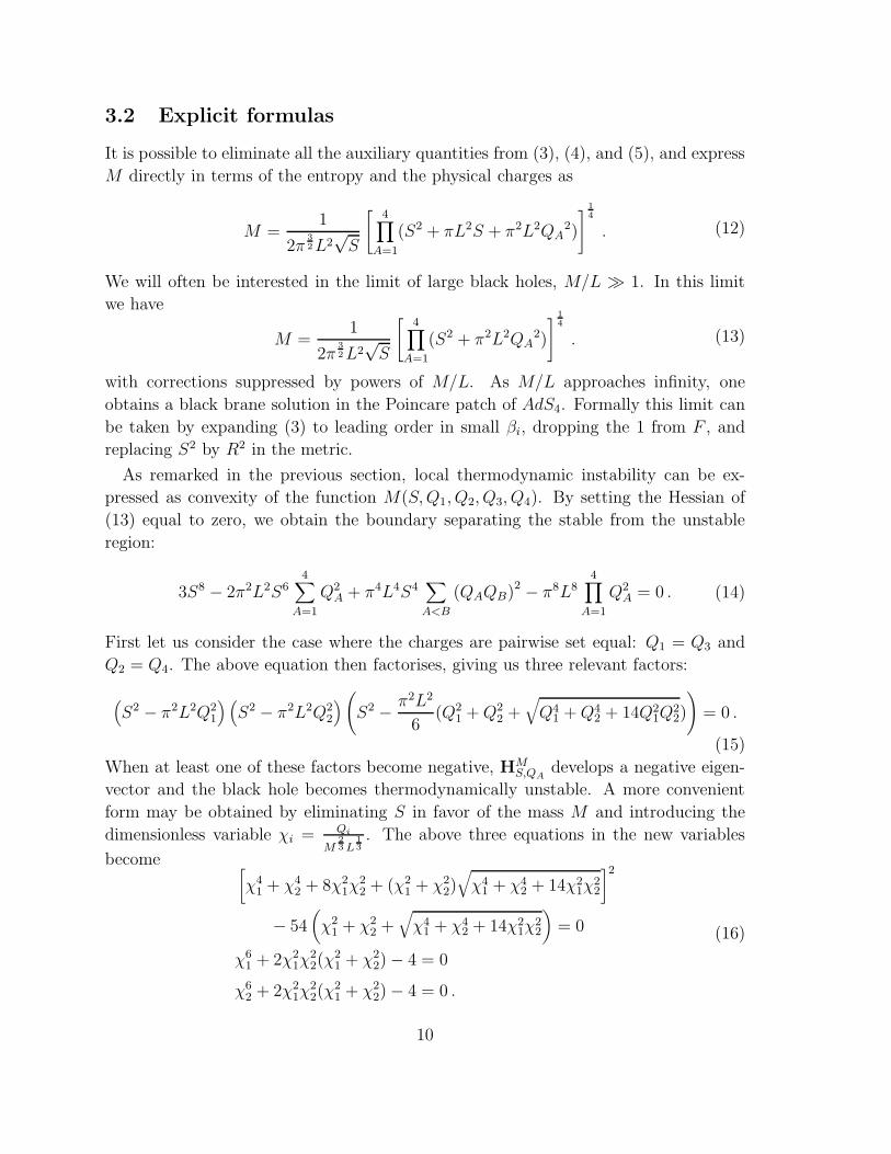
3.2 Explicit formulas

It is possible to eliminate all the auxiliary quantities from (3), (4), and (5), and express

M directly in terms of the entropy and the physical charges as

M =1

2π3

2L2√S

[

4∏

A=1

(S2 + πL2S + π2L2QA2)

]

1

4

. (12)

We will often be interested in the limit of large black holes, M/L ≫ 1. In this limit

we have

M =1

2π3

2L2√S

[

4∏

A=1

(S2 + π2L2QA2)

]

1

4

. (13)

with corrections suppressed by powers of M/L. As M/L approaches infinity, one

obtains a black brane solution in the Poincare patch of AdS4. Formally this limit can

be taken by expanding (3) to leading order in small βi, dropping the 1 from F , and

replacing S2 by R2 in the metric.

As remarked in the previous section, local thermodynamic instability can be ex-

pressed as convexity of the function M(S,Q1, Q2, Q3, Q4). By setting the Hessian of

(13) equal to zero, we obtain the boundary separating the stable from the unstable

region:

3S8 − 2π2L2S64∑

A=1

Q2A + π4L4S4

∑

A<B

(QAQB)2 − π8L8

4∏

A=1

Q2A = 0 . (14)

First let us consider the case where the charges are pairwise set equal: Q1 = Q3 and

Q2 = Q4. The above equation then factorises, giving us three relevant factors:

(

S2 − π2L2Q21

) (

S2 − π2L2Q22

)

(

S2 − π2L2

6(Q2

1 +Q22 +

√

Q41 +Q4

2 + 14Q21Q

22)

)

= 0 .

(15)

When at least one of these factors become negative, HMS,QA

develops a negative eigen-

vector and the black hole becomes thermodynamically unstable. A more convenient

form may be obtained by eliminating S in favor of the mass M and introducing the

dimensionless variable χi =Qi

M2

3L1

3

. The above three equations in the new variables

become[

χ41 + χ4

2 + 8χ21χ

22 + (χ2

1 + χ22)√

χ41 + χ4

2 + 14χ21χ

22

]2

− 54(

χ21 + χ2

2 +√

χ41 + χ4

2 + 14χ21χ

22

)

= 0

χ61 + 2χ2

1χ22(χ

21 + χ2

2)− 4 = 0

χ62 + 2χ2

1χ22(χ

21 + χ2

2)− 4 = 0 .

(16)

10

The region depicting thermodynamically stable black holes is the intersection of the

areas under the 3 curves as shown in figure 2(a).

The other relevant curve is the one separating nakedly singular solutions from regular

black holes. The mathematical criterion for having a regular black hole solution is that

the polynomial F in (3) should have a zero. In the large black hole limit, and in terms

of χ1 and χ2, this criterion reduces to

χ21χ

22(χ

81 + χ8

2)− 4χ41χ

42(χ

41 + χ4

2) + 132χ21χ

22(χ

21 + χ2

2)− 4(χ61 + χ6

2) + 6χ61χ

62 − 432 = 0 .

(17)

To determine if a black hole with given values of mass and charges is unstable, one

first computes the values of χ1 and χ2 and locates this point in figure 2(a). The black

hole is unstable if the point lies outside the shaded region depicting stable black holes

but is within the boundary which separates black holes with naked singularities from

those with a horizon. If the point lies in the unshaded (unstable) region of the plot

without the vector field shown, it means that within each pair one charge wants to

increase while the other decreases. The unstable eigenvector has no components along

the hyperplane Q1 = Q3 and Q2 = Q4 and is not shown.

Finally, let us collect the thermodynamic results for the special case of all charges

equal. We see that thermodynamic instability is present in the narrow region 1 <

χ <√3/22/3. The associated eigenvector has the form (0, 1,−1, 1,−1) where the

components are along the axes M,Q1, Q2, Q3, and Q4 respectively: it looks like one

pair of charges wants to increase while the other decreases. This can happen only

locally, with each of the four charges conserved globally.

We’ll also consider the case in which only two of the charges, Q1 and Q2, are non-

zero. To get the region of thermodynamically stable black holes, we set Q3 = Q4 = 0

in (14):

3S4 − 2π2L2S2(Q21 +Q2

2) + π4L4Q21Q

22 = 0 . (18)

Just as we did in the previous case, we first eliminate S in favor of the mass M and

then introduce the dimensionless variables χi =Qi

M2

3L1

3

to get:

10(χ61 + χ6

2) + 21χ21χ

22(χ

21 + χ2

2)

+(

10χ41 + 10χ4

2 + 26χ21χ

22

)

√

χ41 + χ4

2 − χ21χ

22 − 432 = 0 .

(19)

This is the boundary of the stable region, and is plotted in figure 2(b). Unlike the case

of charges set equal pair-wise, black holes with two charges set to zero always have a

horizon. This may be connected with the fact that there is a limit of rotating M2-branes

with only two independent angular momenta nonzero which is a well-defined multi-

center M2-brane solution, while with all angular momenta nonzero the corresponding

limit is a singular configuration in eleven dimensions [38, 39, 40].

11

For black holes in AdS5 and AdS7, we will simply record here the mass in terms of

the entropy and charges:

AdS5 : M =3

2L2(2π4S)2/3

[

3∏

A=1

(4S2 + π4L2Q2A)

]1/3

AdS7 : M =5

4L2(4π9S)2/5

[

2∏

A=1

(16S2 + π6L2Q2A)

]2/5

.

(20)

Stability analyses similar to the AdS4 case can be carried out for AdS5 and AdS7.

Some work along these lines was presented in [12], but the explicit expressions in (20)

make the calculations much easier.

3.3 Adiabatic evolution

Tracking the evolution of unstable black holes in Lorentzian time is difficult. We have

succeeded in establishing perturbatively the existence of a dynamical instability for

the very special case of all charges equal: this is explained in section 4. This simplest

case required the numerical solution of a fourth order ordinary differential equation

with constraints at the horizon of the black hole and the boundary of AdS4. Most

other cases for black holes in AdS4 involve fluctuations of the metric, which makes

the analysis significantly harder. To investigate the instabilities beyond perturbation

theory would require extensive numerical investigation of the second order PDE’s that

comprise the equations of motion of N = 8 gauged supergravity.

The aim of this section is to use thermodynamic arguments to guess the qualitative

features of the evolution of unstable black holes. Here we focus exclusively on the large

black hole limit; however the conclusions may remain valid to an extent for finite size

black holes with dynamical instabilities. The intuition is that knowing the entropy as

a function of the other extensive parameters amounts to knowing the zero-derivative

terms in an effective Landau-Ginzburg theory of the black hole (or of its dual field

theory representation).

As explained in the paragraph around (9) and (10), an unstable eigenvector ofHSM,QA

(by which we mean one with positive eigenvalue) suggests a direction in which a black

hole solution can be perturbed in order to raise entropy while keeping its total mass

and conserved charges fixed; moreover it was shown in [17] (as we will explain in

section 4) that the black hole’s dynamical instability causes it to evolve in precisely

the direction that the eigenvector indicates. The physics has no infrared cutoff, as is

typical in Gregory-Laflamme setups, so we may hope that the charge and mass densities

vary over long enough distance scales that we may continue to use the most unstable

eigenvector of HSM,QA

locally to determine the direction of the subsequent evolution.

12

Following this line of thought to its logical conclusion leads us to the claim that the mass

density and charge densities will locally evolve, subject to the constraints of conserving

total energy and charge, from their initial values to values along a characteristic curve

of the unstable vector field of HSM,QA

. This can only be approximately correct: finite

wavelength distortions will occur, and it is not precisely right anyway to say that the

time-evolution of Einstein’s equations proceeds so as to maximize black hole entropy.

Nevertheless it seems to us likely that a correct qualitative picture will emerge from

tracking the flows generated by the most unstable eigenvector of HSM,QA

. At late times,

or when charge and mass density are highly concentrated in small regions, another

description is needed.

The characteristic curves of the most unstable eigenvector of HSQ,MA

may terminate

in a region of stability, or in a region of naked singularities. Cosmic Censorship plus the

conjectures of the previous paragraph suggest that the latter should never happen. This

can be checked explicitly for the examples that we have. To this end, one can choose a

generic value of charges and mass so that the black hole is almost naked, then determine

the most unstable eigenvector ofHSM,QA

, and then check that it is tangent to the surface

separating naked singularities from regular black holes. We carried this out numerically

for several cases and verified tangency; however we do not have a general argument. It

appears, in fact, that the normal vector to the surface separating naked singularities

from black holes is a stable eigenvector of HSM,QA

(i.e. its eigenvalue is negative)—at

least in the three-dimensional subspace with Q1 = Q3 and Q2 = Q4—so the obvious

approach to an analytic demonstration that Cosmic Censorship is not violated by

adiabatic evolution of black holes is to show that this normal vector is always a stable

eigenvector of HSM,QA

. For now we content ourselves with the observation that in all

the cases we have checked numerically, adiabatic evolution does stay in the region of

regular black holes.

It is also possible that a characteristic curve becomes unstable at some point, in the

sense that nearby characteristic curves diverge from it. To refine our previous claim,

we may suppose that the black hole evolves along a bundle of nearby characteristic

curves emanating from the original mass and charge density. This bundle may remain

nearly one-dimensional, or it may split or become higher dimensional. We will not

investigate the stability properties of the characteristic curves in any detail. Note that

we are not attempting to specify any spatial or temporal properties of the evolution,

only the range of mass and charge densities which form.

We present in figure 2 plots of unstable eigenvectors of the Hessian matrix HSM,QA

,

projected onto a plane parametrized by two of the charges. From these vector fields,

we may conclude that the different charges exhibit some tendency to separate from one

another, but that this does not always happen, as in the upper right part of figure 2(b).

The crucial point is that the unstable eigenvectors don’t have a component normal

13

to the boundary between naked singularities and regular black holes. Although this

appears obvious from figure 2(a), the plot is slightly misleading in that the eigenvectors

have been projected onto the plane of Q1 = Q3 and Q2 = Q4. One must preserve the

components of vectors in the M direction to verify tangency.

When some angular momenta become large compared to the entropy for a spinning

M2-brane solution, the geometry in eleven dimensions is approximately given by a

rotating multi-center brane solution [38]. If one angular momentum is large, this multi-

center solution is in the shape of a disk; if two are large and equal, it has the shape

of a filled three-sphere. It seems clear that solutions of this form in an asymptotically

flat eleven-dimensional spacetime are unstable toward fragmentation in the directions

transverse to the M2-brane. This would mean that anti-de Sitter space fragments. In

terms of the SU(N) gauge theory, the disk corresponds to a U(1)N−1 Higgsing, and

in the fragmentation process some groups of U(1)’s try to come together to partially

restore gauge invariance. It is not certain that such fragmentation occurs, particularly

if the angular momentum density is large only locally. We merely indicate it as a

possibility in the complicated late-time evolution of unstable black holes.

Finally, it is possible that the unstable black holes evolve to a some new stationary

solution, presumably with a non-uniform horizon. No such solutions are known. It

seems to us most likely that, upon becoming unstable, black holes in AdS undergo an

evolution which eventually produces large curvatures.

4 Existence of a dynamical instability

The existence of dynamical instabilities for thermodynamically unstable black branes

should be completely generic. However, as mentioned already, the stability analysis is

technically complicated for the general case of unequal charges: perturbations of the

metric, four gauge fields, and three scalars lead to difficult coupled partial differential

equations. Here we focus on the AdS4-RN example, where the metric decouples and the

problem can be reduced to a single gauge field and a single scalar. A formal argument

relating thermodynamic and dynamical instability was suggested in [17], using the

identification of the free energy with the Euclidean supergravity action; however we

have not yet succeeded in making this argument rigorous.

Because the unstable eigenvectors of HSM,QA

(for all charges equal and sufficiently

large) do not involve any change in the mass density, it is natural to expect that the

perturbations that give rise to an unstable mode do not involve the metric.10 More

precisely, because of the form of the unstable eigenvectors, we expect that a relevant

10Indeed, we suspect that the decoupling of the metric is possible precisely when there is an eigen-value of HS

M,QAwhich does not have a component in the M direction.

14

perturbation is

δFA = αiAδF (21)

for some δF and fixed i, where the αiA were defined in (2). In section 3 we saw explicitly

that δQ1 = δQ3 = −δQ2 = −δQ4 gave an unstable eigenvector; now we make a trivial

alteration and focus on δQ1 = δQ2 = −δQ3 = −δQ4. Correspondingly we set i = 1 in

(21).

The spectrum of linear perturbations to charged black holes in AdS has been consid-

ered before [41], but for the most part the perturbations under study were minimally

coupled scalars. It is impractical to sift through the entire spectrum of supergravity

looking for unstable modes (or tachyonic glueballs, in the language of [41]). The point

of the previous paragraphs is that thermodynamics provides guidance not only on when

to expect an instability, but also in which mode.

It is straightforward to start with the lagrangian in (2) and show that linearized

perturbations to the equations of motion result in the following coupled equations:

dδF = 0 d ∗ δF + dδϕ1 ∧ ∗F = 0[

+2

L2− 8F 2

µν

]

δϕ1 − 16F µνδFµν = 0 .(22)

Here = gµν∇µ∂ν is the usual scalar laplacian. F in (22) is the background field

strength in (6): it is the common value of the four FA. δF is not the variation in

F itself; rather, the variation of the FA is expressed in terms of δF in (21), with

i = 1. The variation of the field strength is in a direction orthogonal to the background

field strength of the AdS4-RN solution. The graviton decouples from the linearized

perturbation equations: δTµν vanishes at linear order in δF because δFA · FA = 0.11

For comparison, we write down the linearized equations for fluctuations of the other

scalars:[

+2

L2− 8F 2

µν

]

δϕi = 0 (23)

for i = 2, 3. It was shown in [18] that any perturbation involving only matter fields

satisfying the dominant energy condition could not result in a normalizable unstable

mode (that is, a normalizable mode which grows exponentially in Lorentzian time). It

was conjectured [18, 19] that in fact there was no classical instability at all. The scalars

ϕi do not satisfy the dominant energy condition because of the potential term in (2).

Thus the outcome of our calculations is not fore-ordained by general arguments, and

we have a truly non-trivial check on the classical stability of highly charged black holes

in N = 8 gauged supergravity. In fact, our results turn out to be in conflict with the

claim of classical stability in [18, 19].11Besides the all-charges-equal case, we know of one other case where the metric decouples at linear

order: Q1 = Q3 with Q2 = Q4 = 0. There may be other cases as well—presumably wheneverQA · δQA = 0 and δS = 0 for an unstable eigenvector (δS, δQA) of H

MS,QA

.

15

Decoupling the equations in (22) is a chore greatly facilitated by the use of the dyadic

index formalism introduced in [42]. For the reader interested in the details, we present

an outline of the derivation in section 4.1. The final result is the fourth order ordinary

differential equation (ODE)

(

ω2

f+ ∂rf∂r −

ℓ(ℓ+ 1)

r2

)

r3(

ω2

f+ ∂rf∂r −

ℓ(ℓ+ 1)

r2− 2M

r3+

4Q2

r4

)

rδϕ1(r) =

4Q2

(

ω2

f+ ∂rf∂r

)

δϕ1(r) ,

(24)

where we have assumed the separated form δϕ1 = Re e−iωtYℓmδϕ1(r), where Yℓm is the

usual spherical harmonic on S2. This is to be compared with the separated equation

for the other scalars:(

ω2

f+ ∂rf∂r −

ℓ(ℓ+ 1)

r2− 2M

r3+

4Q2

r4

)

rδϕi(r) = 0 (25)

for i = 2, 3.

4.1 Dyadic index derivation of (24)

To derive (24) using the dyadic index formalism, it is convenient first to switch to

+−−− signature to avoid sign incompatibilities between the raising and lowering of

dyadic and vector indices. One introduces a null tetrad of vectors, (lµ, nµ, mµ, mµ),

defined so that lµnµ = −mµmµ = 1 and all other inner products vanish. Next define

σµ

∆∆=(

lµ mµ

mµ nµ

)

(26)

and set D = lµ∂µ, ∆ = nµ∂µ, δ = mµ∂µ, δ = mµ∂µ. Vector indices are converted into

dyadic indices by setting v∆∆ = σµ

∆∆vµ. Dyadic indices are raised and lowered using

northwest contraction rules with ǫ01 = ǫ01 = ǫ01 = ǫ01 = 1. By demanding that σµ

∆∆

is covariantly constant, one can obtain a unique covariant derivative Dµ, whose action

on a spinor is

DµψΓ = ∂µψΓ − ψΣγµΣΓ . (27)

The so-called spin coefficients, γ∆∆ΣΓ = σµ

∆∆γµΣΓ, are conventionally written as

γ00ΣΓ =(

κ ǫǫ π

)

γ01ΣΓ =(

σ ββ µ

)

γ10ΣΓ =(

ρ αα λ

)

γ11ΣΓ =(

τ γγ ν

)

.

(28)

16

A less compressed presentation of dyadic index formalism can be found in [42, 43], and

the appendix to [44].

For AdS4-RN, a convenient choice of the null tetrad and the corresponding nonzero

spin coefficients are as follows:

lµ = (1/f, 1, 0, 0) nµ =1

2(1,−f, 0, 0)

mµ =1

r√2(0, 0, 1, i csc θ) mµ =

1

r√2(0, 0, 1,−i csc θ)

(29)

ρ = −1

rµ = − f

2rγ =

f ′

4α = −β = −cot θ√

8r. (30)

in (29) and (30) we have not yet taken the black brane limit. Taking this limit replaces

csc θ by 1 in (29) and sets α = β = 0 in (30). Proceeding without the black brane

limit, we trade the real antisymmetric tensor Fµν for a complex symmetric tensor,

Φ(0)∆Γ =

(

φ(0)0 φ

(0)1

φ(0)1 φ

(0)2

)

(31)

through the formula

4√2Fµνσ

µ

∆∆σνΓΓ = Φ

(0)∆Γǫ∆Γ + Φ

(0)

∆Γǫ∆Γ . (32)

The factor of 4√2 in (31) is for convenience: the AdS4-RN background has φ

(0)1 = Q/r2

and all other components zero. In the same way we trade in δFµν for Φ∆Γ, whose

components are φ0, φ1, and φ2, with a similar factor of 4√2. Finally, we write ϕ in

place of δϕ1 to avoid the ambiguity in the meaning of δ.

The first order equations for the gauge field in (22) can now be cast in dyadic form

as follows:

D∆ΓΦ∆Γ +

1

2∂∆∆ϕ(Φ

(0)∆Γǫ∆Γ + Φ

(0)

∆Γǫ∆Γ) = 0 . (33)

In components, these equations read

(D − 2ρ)φ1 − (δ − 2α)φ0 = −φ(0)1 Dϕ

(∆ + µ− 2γ)φ0 − δφ1 = 0

(D − ρ)φ2 − δφ1 = 0

(δ + 2β)φ2 − (∆ + 2µ)φ1 = φ(0)1 ∆ϕ .

(34)

It is possible to combine these equations into three second order equations in which only

a single φi appears. Together with the scalar equation, these equations are equivalent

17

to (22):[

(D − 3ρ)(∆ + µ− 2γ)− δ(δ − 2α)]

φ0 = −φ(0)1 δDϕ

[

(∆ + 3µ)(D − ρ)− δ(δ + 2β)]

φ2 = −φ(0)1 δ∆ϕ

[

(D − 2ρ)(∆ + 2µ)− (δ + β − α)δ]

φ1 = −φ(0)1 D∆ϕ

[

+2

L2+ 2(φ

(0)1 )2

]

ϕ = −4φ(0)1 Reφ1

(35)

where we have made use of the fact that the spin coefficients are all real for AdS4-

RN. The equations (34) are a special case of (3.1)-(3.4) of [45]. The first and second

equations of (35) are (3.5) and (3.7) of [45], and the third is derived in a similar manner.

The fourth is the scalar equation in (22), but to preserve the definition of we write

= −gµν∇µ∂ν in +−−− conventions. The differential operators in the third equation

of (35) are purely real (this takes a bit of checking for (δ + β − α)δ), so we can take

the real and imaginary parts of this equation. The equation for Imφ1 decouples from

all the others. The equations for φ0 and φ2 are sourced by ϕ, but φ0 and φ2 do not

otherwise enter; thus one can solve first for Reφ1 and ϕ, and afterwards use the first

and second equations in (35) to obtain φ0 and φ2. Since φ(0)1 is nowhere vanishing, the

last equation in (35) can be used to eliminate Reφ1 algebraically. The final result is

[

(D − 2ρ)(∆ + 2µ)− (δ + β − α)δ] 1

4φ(0)1

[

+2

L2+ 2(φ

(0)1 )2

]

ϕ = φ(0)1 D∆ϕ . (36)

Plugging in the separated ansatz ϕ = Re e−iωtYℓmδϕ1(r), one easily obtains (24).

4.2 Numerical results from the fourth order equation

A dynamical instability exists if there is a normalizable, unstable solution to (24)

or to (25). Neither of these equations admits a solution in closed form, so we have

resorted to numerics. Briefly, the conclusion is that, in the black brane limit and within

the limits of numerical accuracy, we find a single unstable mode for (24) precisely

when χ > 1, and no instabilities for (25). This is completely in accord with the

intuition from thermodynamics: (25) represents a fluctuation that has nothing to do

with the variation of charges that gave the unstable eigenvector of the Hessian matrix

of M(S,Q1, Q2, Q3, Q4). The unstable mode in (24) persists to finite size AdS4-RN

black holes, but eventually disappears for small enough black holes.

To carry out a numerical study of (24), the first step is to cast the equation in terms of

a dimensionless radial variable u, a dimensionless charge parameter χ, a dimensionless

mass parameter σ, and a dimensionless frequency ω:

u =r

M1/3L2/3χ =

Q

M2/3L1/3σ =

(

L

M

)2/3

ω =ωL4/3

M1/3. (37)

18

Then we have(

ω2

f+ ∂uf∂u − σ

ℓ(ℓ+ 1)

u2

)

u3(

ω2

f+ ∂uf∂u − σ

ℓ(ℓ+ 1)

u2− 2

u3+

4χ2

u4

)

uδϕ1 =

4χ2

(

ω2

f+ ∂uf∂u

)

δϕ1

f = σ − 2

u+χ2

u2+ u2 .

(38)

Evidently, the dimensionless control parameters are ℓ (the partial wave number), σ,

and χ. Using Mathematica, we solved (38) numerically via a shooting method, and

obtained wavefunctions δϕ1(r) which fall off like 1/r2 near the boundary of AdS4 and

at least as fast as (r − rH)|ω|/f ′(rH ) near the horizon.

To check that the wavefunction is well behaved near the horizon12 let us transform

to Kruskal coordinates. The metric near the horizon is

ds2 ≈ −f ′(rH)(r − rH)dt2 +

dr2

f ′(rH)(r − rH)+ r2HdΩ

22 , (39)

where rH is the radius of the horizon. Dropping the S2 piece and introducing a tortoise

coordinate r∗, null coordinates P±, and Kruskal coordinates (T,R) according to

dr∗dr

=1

f ′(rH)(r − rH)

P± = e1

2f ′(rH )(±t+r∗) = ±T +R ,

(40)

one finds that the near-horizon metric is indeed regular:

ds22 = −f ′(rH)(r − rH)dt2 +

dr2

f ′(rH)(r − rH)=

4

f ′(rH)(−dT 2 + dR2) . (41)

Having a radial wavefunction δϕ1(r) = (r − rH)|ω|/f ′(rH )ρ(r − rH), where ρ(r − rH)

remains bounded at the horizon, means that the time-dependent perturbation (with

angular dependence suppressed) is

δϕ1(t, r) ∼ (r − rH)|ω|/f ′(rH )e|ω|tρ(r − rH) ∼ P

2|ω|/f ′(rH )+ ρ(P+P−) , (42)

which remains bounded as P− → 0. The black hole horizon is at P− = 0, P+ > 0

(see figure 3). Thus we see that the perturbation is small at the horizon in good

coordinates, at least for small P+. (As the perturbation grows, the horizon eventually

starts to fluctuate, but this is not an issue in the question of whether the instability

exists).

12We thank G. Horowitz for suggesting that this check should be made.

19

A qualitative summary of our numerical results is displayed in figure 4(a). An

example of a normalizable wave-function with negative ω2 is shown in figure 4(b).

Some points to note are:

• The boundary of the region of dynamical stability comes from instability in the

ℓ = 1 mode. The ℓ = 0 mode is projected out by charge conservation. Higher ℓ

modes become unstable in the upper left part of the shaded triangle in figure 4(b).

The boundaries of dynamical instability for different ℓ all come together at σ = 0.

• At σ = 0, thermodynamic stability is lost at χ = 1, whereas dynamical instability

sets in at χ = 1.007. We believe that the 0.7% discrepancy is due to numerical

error.

• We have drawn the regions of dynamical instability and thermodynamic stability

as disjoint in figure 4(a). In fact, our current numerics shows them overlapping

by about 0.1% around σ = 0.1. We do not view this as significant because the

numerical errors seem to be around 1%.

Finally, it is worth pointing out that the string theory program of computing black

hole entropy via a microscopic state count in a field theory dual (see for example [46],

or [47] for a review) has proved hard to extend past the boundaries of thermodynamic

stability. For instance, we have a good understanding of the entropy of near-extremal

D3-branes [48, 49], but not of small Schwarzschild black holes in AdS. It seems to us

that this is no accident: most sensible field theories have log-convex partition functions,

and this translates into Hessian matrices HSM,QA

which have no negative eigenvalues.

Pushing past the boundary of thermodynamic stability in a field theory may be possible

(particularly as one crosses a phase boundary and begins to nucleate the new phase),

but doing so seems likely to produce dynamical instabilities in the Lorentzian time-

evolution. This point of view has indeed informed our entire investigation.

A dual field theory description of a small Schwarzschild black hole in AdS must in-

volve thermodynamic instability but no dynamical instabilities. We believe that finite

volume effects in the field theory are essential in this regard: if one imagines a Landau-

Ginzburg effective description of the field theory, then derivative terms must restore

stability to a system whose infrared tendencies are controlled by the thermodynamic

instability. Various properties of small AdS-Schwarzschild black holes have been ex-

plored (see for example [50, 51]), but the basic problem of reconciling thermodynamic

instability with dynamical stability in the presence of a field theory dual remains to be

addressed.

20

5 Conclusions

A common conception of the Gregory-Laflamme instability is that a uniform solution

to Einstein’s equations (plus matter) competes with a non-uniform solution, and the

non-uniform solution sometimes wins out entropically. In such a situation, the generic

expectation is that there is a first order tunneling transition from the uniform to the

non-uniform state, which may take place very slowly due to a large energetic barrier.

In fact, the original papers [1, 2] focused mainly on demonstrating the existence of

unstable modes in a linearized perturbation analysis of the uniform solution. The

distinction is between global and local stability. At the level of classical gravity/field

theory, the latter concept is more meaningful, because with quantum effects suppressed

it is impossible to tunnel away from a locally stable solution. The aim of this paper and

its shorter companion paper [17] has been to study local dynamical stability of black

holes in anti-de Sitter space in relation to a particular notion of local thermodynamic

stability, namely downward concavity of the entropy as a function of the other extensive

variables. We reach two main conclusions:

1. In the limit of large black holes in AdS, dynamical and thermodynamic stability

coincide. This conclusion is supported by numerical evidence. The small discrep-

ancy between the observed onset of dynamical and thermodynamic instabilities

is probably numerical error.

2. Dynamical instabilities persist for finite size black holes in AdS, down to horizon

radii on the order of the AdS radius. The evidence is again only numerical, but

we believe the final answer is correct and robust.

We regard point 1 as a partial verification of a rather more general conjecture, namely

that black branes should have Gregory-Laflamme instabilities (in the local, dynamical

sense of the original papers [1, 2]) precisely when thermodynamic stability is lost.

Point 2 is surprising because it is the first known example of a stationary black hole

solution with a point-like singularity which exhibits a dynamical Gregory-Laflamme

instability. Furthermore, it shows that no-hair theorems cannot always hold in anti-de

Sitter space. Black branes which experience a Gregory-Laflamme instability are often

supposed to split their horizons and fall into pieces. For this to happen to a horizon

whose topology is S2 and which cloaks a point-like singularity would be truly novel:

what could tear apart a point-like singularity?

21

Is Cosmic Censorship really threatened by our analysis?13 It is too early to say.

Using the heuristic method of calculating the most unstable eigenvector of the Hessian

of the entropy function, we have argued that adiabatic evolution of unstable black holes

does not lead to nakedly singular solutions. However this does not bear directly on

the question of whether the horizon should split as it is assumed to do in the evolution

of unstable black branes. We leave open many questions as to the eventual fate of

unstable black holes in AdS: Might they settle down to new non-uniform stationary

solutions? Do regions of strong curvature form? Does the horizon split? Does AdS

itself fragment through a classical process? We leave these issues for future work.

Acknowledgements

We thank C. Callan and A. Chamblin for useful discussions, and H. Reall, T. Prestidge,

and G. Horowitz for other enlightening communications. This work was supported in

part by DOE grant DE-FG02-91ER40671, and by a DOE Outstanding Junior Inves-

tigator award. S.S.G. thanks the Aspen Center for Physics for hospitality during the

early phases of the project.

References

[1] R. Gregory and R. Laflamme, “Black strings and p-branes are unstable,” Phys.

Rev. Lett. 70 (1993) 2837, hep-th/9301052.

[2] R. Gregory and R. Laflamme, “The Instability of charged black strings and

p-branes,” Nucl. Phys. B428 (1994) 399–434, hep-th/9404071.

[3] E. Witten, “Anti-de Sitter space, thermal phase transition, and confinement in

gauge theories,” Adv. Theor. Math. Phys. 2 (1998) 505, hep-th/9803131.

[4] C. Csaki, H. Ooguri, Y. Oz, and J. Terning, “Glueball mass spectrum from

supergravity,” JHEP 01 (1999) 017, hep-th/9806021.

[5] O. Aharony, S. S. Gubser, J. Maldacena, H. Ooguri, and Y. Oz, “Large N field

theories, string theory and gravity,” Phys. Rept. 323 (2000) 183,

hep-th/9905111.

13If asymptotically flat spacetimes are part of the hypothesis of Cosmic Censorship, as is oftenthe case, then of course no demonstration in global anti-de Sitter space is relevant. We prefer abroader interpretation of Cosmic Censorship—loosely speaking, that no observer who follows a timeliketrajectory which never runs into singularities can receive signals from a singularity.

22

[6] J. Maldacena, “The large N limit of superconformal field theories and

supergravity,” Adv. Theor. Math. Phys. 2 (1998) 231–252, hep-th/9711200.

[7] S. S. Gubser, I. R. Klebanov, and A. M. Polyakov, “Gauge theory correlators

from non-critical string theory,” Phys. Lett. B428 (1998) 105, hep-th/9802109.

[8] E. Witten, “Anti-de Sitter space and holography,” Adv. Theor. Math. Phys. 2

(1998) 253–291, hep-th/9802150.

[9] V. Balasubramanian, P. Kraus, and A. Lawrence, “Bulk vs. boundary dynamics

in anti-de Sitter spacetime,” Phys. Rev. D59 (1999) 046003, hep-th/9805171.

[10] S. S. Gubser, “Thermodynamics of spinning D3-branes,” Nucl. Phys. B551

(1999) 667, hep-th/9810225.

[11] M. Cvetic and S. S. Gubser, “Phases of R-charged black holes, spinning branes

and strongly coupled gauge theories,” JHEP 04 (1999) 024, hep-th/9902195.

[12] M. Cvetic and S. S. Gubser, “Thermodynamic stability and phases of general

spinning branes,” JHEP 07 (1999) 010, hep-th/9903132.

[13] R.-G. Cai and K.-S. Soh, “Localization instability in the rotating D-branes,”

JHEP 05 (1999) 025, hep-th/9903023.

[14] T. Harmark and N. A. Obers, “Thermodynamics of spinning branes and their

dual field theories,” JHEP 01 (2000) 008, hep-th/9910036.

[15] A. Chamblin, R. Emparan, C. V. Johnson, and R. C. Myers, “Charged AdS

black holes and catastrophic holography,” Phys. Rev. D60 (1999) 064018,

hep-th/9902170.

[16] A. Chamblin, R. Emparan, C. V. Johnson, and R. C. Myers, “Holography,

thermodynamics and fluctuations of charged AdS black holes,” Phys. Rev. D60

(1999) 104026, hep-th/9904197.

[17] S. S. Gubser and I. Mitra, “Instability of charged black holes in anti-de Sitter

space,” hep-th/0009126.

[18] S. W. Hawking and H. S. Reall, “Charged and rotating AdS black holes and

their CFT duals,” Phys. Rev. D61 (2000) 024014, hep-th/9908109.

[19] S. Hawking, “Stability in ADS and Phase Transitions,” talk at Strings ’99,

http://strings99.aei-potsdam.mpg.de/cgi-bin/viewit.cgi?speaker=Haw-

king.

23

[20] T. Banks, M. R. Douglas, G. T. Horowitz, and E. Martinec, “AdS dynamics

from conformal field theory,” hep-th/9808016.

[21] S. W. Hawking and D. N. Page, “Thermodynamics of black holes in anti-de

Sitter space,” Commun. Math. Phys. 87 (1983) 577.

[22] D. J. Gross, M. J. Perry, and L. G. Yaffe, “Instability of flat space at finite

temperature,” Phys. Rev. D25 (1982) 330–355.

[23] T. Prestidge, “Dynamic and thermodynamic stability and negative modes in

Schwarzschild-anti-de Sitter,” Phys. Rev. D61 (2000) 084002, hep-th/9907163.

[24] T. Prestidge, “Making $ense of the information loss paradox,”. D.Phil. thesis,

Cambridge University, January 2000.

[25] C. S. Peca and J. P. S. Lemos, “Thermodynamics of Reissner-Nordstroem

anti-de Sitter black holes in the grand canonical ensemble,” Phys. Rev. D59

(1999) 124007, gr-qc/9805004.

[26] C. S. Peca and J. P. S. Lemos, “Thermodynamics of toroidal black holes,” J.

Math. Phys. 41 (2000) 4783–4789, gr-qc/9809029.

[27] R. H. Price, “Nonspherical perturbations of relativistic gravitational collapse. 1.

Scalar and gravitational perturbations,” Phys. Rev. D5 (1972) 2419–2438.

[28] S. B. Giddings, J. A. Harvey, J. G. Polchinski, S. H. Shenker, and A. Strominger,

“Hairy black holes in string theory,” Phys. Rev. D50 (1994) 6422–6426,

hep-th/9309152.

[29] D. Sahakian, to appear.

[30] M. Berkooz and M. Rozali, “Near Hagedorn dynamics of NS fivebranes, or a new

universality class of coiled strings,” JHEP 05 (2000) 040, hep-th/0005047.

[31] T. Harmark and N. A. Obers, “Hagedorn behaviour of little string theory from

string corrections to NS5-branes,” Phys. Lett. B485 (2000) 285–292,

hep-th/0005021.

[32] V. Kazakov, I. Kostov, and D. Kutasov, to appear.

[33] B. de Wit and H. Nicolai, “N=8 supergravity with local SO(8) X SU(8)

invariance,” Phys. Lett. B108 (1982) 285.

[34] B. de Wit and H. Nicolai, “N=8 supergravity,” Nucl. Phys. B208 (1982) 323.

24

[35] B. de Wit and H. Nicolai, “The consistency of the S7 truncation in d = 11

supergravity,” Nucl. Phys. B281 (1987) 211.

[36] M. J. Duff and J. T. Liu, “Anti-de Sitter black holes in gauged N = 8

supergravity,” Nucl. Phys. B554 (1999) 237, hep-th/9901149.

[37] J. Maldacena, J. Michelson, and A. Strominger, “Anti-de Sitter fragmentation,”

JHEP 02 (1999) 011, hep-th/9812073.

[38] P. Kraus, F. Larsen, and S. P. Trivedi, “The Coulomb branch of gauge theory

from rotating branes,” JHEP 03 (1999) 003, hep-th/9811120.

[39] D. Z. Freedman, S. S. Gubser, K. Pilch, and N. P. Warner, “Continuous

distributions of D3-branes and gauged supergravity,” JHEP 07 (2000) 038,

hep-th/9906194.

[40] M. Cvetic, S. S. Gubser, H. Lu, and C. N. Pope, “Symmetric potentials of

gauged supergravities in diverse dimensions and Coulomb branch of gauge

theories,” Phys. Rev. D62 (2000) 086003, hep-th/9909121.

[41] C. Csaki, Y. Oz, J. Russo, and J. Terning, “Large N QCD from rotating branes,”

Phys. Rev. D59 (1999) 065012, hep-th/9810186.

[42] E. Newman and R. Penrose, “An Approach to gravitational radiation by a

method of spin coefficients,” J. Math. Phys. 3 (1962) 566–578.

[43] R. M. Wald, General Relativity. Chicago University Press, Chicago, 1984.

[44] S. S. Gubser, “Absorption of photons and fermions by black holes in four

dimensions,” Phys. Rev. D56 (1997) 7854–7868, hep-th/9706100.

[45] S. A. Teukolsky, “Perturbations of a rotating black hole. 1. Fundamental

equations for gravitational, electromagnetic, and neutrino field perturbations,”

Astrophys. J. 185 (1973) 635–647.

[46] A. Strominger and C. Vafa, “Microscopic Origin of the Bekenstein-Hawking

Entropy,” Phys. Lett. B379 (1996) 99–104, hep-th/9601029.

[47] A. W. Peet, “TASI lectures on black holes in string theory,” hep-th/0008241.

[48] S. S. Gubser, I. R. Klebanov, and A. W. Peet, “Entropy and Temperature of

Black 3-Branes,” Phys. Rev. D54 (1996) 3915–3919, hep-th/9602135.

[49] A. Strominger, unpublished, 1996.

25

[50] G. T. Horowitz and V. E. Hubeny, “Quasinormal modes of AdS black holes and

the approach to thermal equilibrium,” Phys. Rev. D62 (2000) 024027,

hep-th/9909056.

[51] G. T. Horowitz and V. E. Hubeny, “CFT description of small objects in AdS,”

JHEP 10 (2000) 027, hep-th/0009051.

S

M

BA

inflection point

FIGURES

Figure 1: An example of a mass function whose convex hull is flat. The region weinterpret as stable is from A to B.

26

Q = Q1 3

Q =

Q2

4

Q1

0 0.5 1 1.5 20

0.5

1

1.5

2

0 1 2 3 40

1

2

3

4

Nakedsingularities

(a) (b)

stable

stable

Q2

Figure 2: Plots of the most unstable eigenvector of the Hessian matrix ofS(M,Q1, Q2, Q3, Q4). The inner curves are boundaries of stability. The outer curves(when they are present) denote the boundary between regular black branes and nakedsingularities.

T P

P-

+

R

AdS

horiz

on

singularity

Figure 3: The Penrose diagram of a regular AdS black hole. We can take T = R =P+ = P− = 0 at the center of the diagram. The black hole horizon is the diagonal linegoing up and right from the origin.

27

unstable

stable

unstable

unstable

stable

stable

dynamicallythermodynamically

highlycharged

σ

χ

large AdS-Schwarzschild

small AdS-Schwarzschild

uncharged

Nakedsingularities

AdSwithinAdS 4

2

a)

1~δφ

2 4 6 8 10

0.2

0.4

0.6

0.8

u

b)

Figure 4: (a) A topologically correct representation of dynamical and thermodynamicstability in the whole χ-σ plane (but see the text regarding possible overlap of thetwo shaded regions). (b) A sample normalizable wave-function with negative ω2: hereσ = 0.3, χ = 0.96, and ω2 = −0.281.

28