arX

iv:a

stro

-ph/

9704

243v

2 7

Oct

199

7

Determination of the Primordial Magnetic Field Power Spectrum

by Faraday Rotation Correlations

Tsafrir Kolatt1

Harvard-Smithsonian Center for Astrophysics, 60 Garden St., Cambridge, MA 02138and

The Physics Department and Lick Observatory, UCSC, Santa-Cruz, CA 95064

ABSTRACT

This paper introduces the formalism which connects between rotation measure (RM)

measurements for extragalactic sources and the cosmological magnetic field power spec-

trum. It is shown that the amplitude and shape of the cosmological magnetic field power

spectrum can be constrained by using a few hundred radio sources, for which Faraday

RMs are available. This constraint is of the form Brms<∼ 1 × [2.6 × 10−7cm−3/nb]h

nano-Gauss (nG) on ∼ 10− 50 h−1Mpc scales, with nb the average baryon density and

h the Hubble parameter in 100 km s−1 Mpc−1 units. The constraint is superior to and

supersedes any other constraint which come from either CMB fluctuations, Baryonic

nucleosynthesis, or the first two multipoles of the magnetic field expansion. The most

adequate method for the constraint calculation uses the Bayesian approach to the max-

imum likelihood function. I demonstrate the ability to detect such magnetic fields by

constructing simulations of the field and mimicking observations. This procedure also

provides error estimates for the derived quantities.

The two main noise contributions due to the Galactic RM and the internal RM

are treated in a statistical way following an evaluation of their distribution. For a

range of magnetic field power spectra with power indices −1 ≤ n ≤ 1 in a flat

cosmology (Ωm=1) we estimate the signal-to-noise ratio, Q, for limits on the mag-

netic field Brms on ∼ 50 h−1Mpc scale. Employing one patch of a few square de-

grees on the sky with source number density nsrc, an approximate estimate yields

Q ≃ 3 × (Brms/1nG)(nsrc/50 deg−2)(2.6 × 10−7cm−3/nb)h. An all sky coverage, with

much sparser, but carefully tailored sample of ∼ 500 sources, yields Q ≃ 1 with the

same scaling. An ideal combination of small densely sampled patches and sparse all-sky

coverage yields Q ≃ 3 with better constraints for the power index. All of these estimates

are corroborated by the simulations.

Subject headings: Cosmology: Large-Scale Structure of Universe, Theory – Magnetic

Fields – Polarization – Methods: Statistical

1email:tsafrir@physics.ucsc.edu

– 2 –

1. INTRODUCTION

There is plenty evidence for magnetic fields on the scale of the earth, the solar system, the

interstellar medium, galaxies and clusters of galaxies [for the extragalactic magnetic field see review

by Kronberg (1994, K94) and references therein]. We still don’t know however whether any larger

scale magnetic fields exist. There are various upper limits on the rms value of the cosmological

magnetic field, but the upper limits are still too high to exclude any relevance to magnetic fields

observed on smaller scales. Cosmological magnetic fields might help to resolve the bothersome

question of the origin of the ∼ 10−6G magnetic field which exists on galactic scales or fields of

similar size seen on the scales of galaxy clusters. A primordial (pre – galaxy formation) magnetic

field amplified by the gravitational collapse, and then by processes like differential rotation and

dynamo amplification (Parker 1979), can serve to seed these observed smaller scale magnetic fields.

The most stringent upper limits to date for magnetic fields on cosmological scales come from

three different sources:

1. Big Bang Baryonic Nucleosynthesis (BBN).

Magnetic fields that existed during the BBN epoch would affect the expansion rate, the

reaction rates, the electron density (and possibly the space-time geometry). By taking all

these effects into account in the calculation of the element abundances, and then comparing

the results with the observed abundances one can set limits on the magnetic field amplitude.

The limits for homogeneous magnetic fields on scales ≫ 10−14 h−1Mpc (distances are quoted

in comoving coordinates) and up to the BBN horizon size (∼ 10−4 h−1Mpc) are 10−9 − 10−6

G in terms of today’s values (Grasso & Rubinstein 1995, 1996 ; Cheng, Olinto, Schramm, &

Truran 1996). The relevance of these limits for the maximum value of magnetic field seeds on

the subgalactic scale is obvious, but in order for these limits to be relevant to the intergalactic

magnetic field, further assumptions about the super-horizon magnetic field power spectrum

and the magnetic field generation epoch should be made.

2. The CMB radiation.

The presence of magnetic fields during the time of decoupling causes anisotropy, i.e. different

expansion rates in different directions (Zel’dovich & Novikov 1975). Masden (1989) provides

a useful formula for the connection between the measured temperature fluctuations on a given

scale at zd, the decoupling time, and the limits on the equivalent scale today. For a magnetic

field energy density much smaller than the matter energy density, the limit is

Brms(R) ≤ 3× 10−4h

√∆TT (R)Ω

√1 + zd

G . (1)

For typical values of h = 1 (the Hubble constant in units of 100 km s−1 Mpc−1), temperature

fluctuations of ∼ 10−5, Ω = 1 and zd ≃ 103 the limit becomes Brms < 10−8−10−9G. Recently,

Barrow, Frreira, & Silk (1997) used the COBE 4-year data to constrain the magnetic field on

the horizon scale by B(R = Rh) < 6.8(Ωh2)1/2 nG.

– 3 –

3. Multipole expansion of RM observations.

Passing through a magnetoionic medium, polarized light undergoes rotation of the polariza-

tion vector (Faraday rotation, for definition see §2). The rotation amount is proportional to

the dot product of the magnetic field and the light propagation direction, and to the distance

the light travels through the medium. If any cosmological magnetic field exists, the farther

away the source, the more the polarized light component is rotated. We refer to this as the

“monopole” term. This term exists even if the field has no preferred direction on the horizon

scale, namely even without breaking the isotropy hypothesis.

If there is a preferred direction to the field on a cosmological scale, a dipole will show up in

the RM measurements across the sky, due to the different sign of the dot product (and thus

the different rotation direction). So far attempts have been made only to identify a monopole

or a dipole in the magnetic field for scales of z ≃ 2.5 (Kronberg 1976) and z ≃ 3.6 (Vallee

1990). The search for a dipole signature in the Faraday rotation values for a sample of extra-

galactic sources (QSO) yields limits of B < 1−10−1 nG depending on the assumed cosmology

(Kronberg & Simard-Normandin 1976, Kronberg 1976). Vallee (1990) tried to estimate the

limits on the dipole and the monopole terms and concluded that an all-prevailing (up to

z = 3.6) field must be smaller than 6× 10−2[10−6cm−3

nb

]nG .

Other potential methods of detecting a possible cosmological magnetic field include distortion of the

acoustic (“Doppler”) peak in the CMB power spectrum (Adams, Danielsson, Grasso, & Rubinstein

1996) and Faraday rotation of the CMB radiation polarized components (Loeb & Kosowsky 1996).

These methods where not designed to probe any magnetic field generated after recombination.

Their implementation is still pending on the upcoming measurements of the CMB fluctuations and

polarization.

A method that does probe magnetic fields generated in the post recombination era, relies on

cosmic ray (CR) detection. The effect of magnetic fields on high energy CRs (> 1018 eV) is twofold.

It will first alter the energy distribution of CRs (Lee, Olinto, & Sigl 1995, Waxman & Miralda-

Escude 1996) and then, if the CR direction is identified and attributed to a known region or source,

the magnetic field either smears the directionality (for field coherent scales much smaller than the

distance to the source) or deflects the CR direction from aligning with the source direction. Current

limits from this last effect are either very weak or non-existing.

Theories for primordial magnetic fields in the framework of structure evolution paradigms

have been suggested by a number of authors. Magnetic fields on cosmological scales emerge in the

framework of these theories in one of three epochs: the inflation era, the plasma era, and the post-

recombination era. In the inflation era, magnetic fields form due to quantum mechanical processes

(Turner & Widrow 1988; Quashnock, Loeb, & Spergel 1989, Vachaspati 1991, Ratra 1992a, 1992b,

Dolgov & Silk 1993) or possibly magneto-hydrodynamics (Brandenburg, Enquist, & Olesen 1996).

During the plasma era, prior to recombination, magnetic fields form due to vorticity caused by

the mass difference between the electron and the proton (Harrison 1973, but see Rees 1987), or

where magnetic field fluctuation survival (no vorticity assumed) depends on the fluctuation scale

– 4 –

(Tajima et al. 1992). Other authors have pointed out that even in the post recombination era

(but before galaxy formation) magnetic fields can be generated by tidal torques (Zweibel 1988), or

by cosmic strings wakes (Ostriker & Thompson 1987, Thompson 1990). Magnetic field generated

in the process of structure formation itself, due to falling matter (Pudritz & silk 1989), or star

burst regions, are less likely to feed back into the intergalactic space and to affect the cosmological

magnetic field. Nevertheless, proposals in this spirit were also considered by taking into account

wind driven plasma which fills intergalactic space with magnetic fields.

Whatever the origin of cosmological magnetic fields, each suggested theory, specifies the mag-

netic field amplitude and power spectrum shape. Thus, each of the theories can in principle become

refutable if we could measure, or put limits on, the normalized power spectrum of the cosmological

magnetic field.

This challenge and the realization that with existing or upcoming data, it will be possible to

measure the magnetic field power spectrum has led us to develop a method for doing so. We argue

that much better estimates (or upper limits) for the cosmological magnetic field can be calculated

by using the RM correlation matrix.

All previous attempts to limit the cosmological magnetic field dipole on very large scales

(z ≃ 2.5 − 3.6), suffer from two drawbacks. From a theoretical point of view it is difficult to

reconcile the necessary anisotropy such a dipole imposes with other evidence which suggest global

isotropy. From a practical point of view, this test is confined to one scale, and doesn’t allow

measurements over a whole range. Only by extending the measurement to a whole range, can one

estimate the full power spectrum (PS). Although contribution from a “random walk” can be useful

even if only a monopole is calculated (see below), the information is partial, inferior to the full

derivation of the magnetic field by RM correlations, and sensitive to evolutionary effects.

Why is the correlation approach more advantageous than other type of statistics and in partic-

ular why is it better than the monopole approach? In the monopole approach we are looking for a

correlation between RM values and the source redshift. Let’s pretend at first that all measurements

are exact and there are no noise sources (we’ll notice in §3 that these two assumptions are far too

optimistic). Consider a scale l0 over which the magnetic field is coherent with an rms value of

Brms. A line-of-sight to a source at a distance rsrc will cross Nl = rsrc/l0 such regions. There is no

correlation in the magnetic field orientation between the regions, and on average each one of them

contributes RMirms ∝ Brmsl0. The overall contribution due to Nl random walk steps sums up to

RMrms =√NlRM

irms ∝ Brms

√l0rsrc . It is thus clear that the larger rsrc, the bigger RMrms we

expect for an ensemble of sources located at rsrc . Now let’s turn to the correlation approach. Two

lines-of-sight to two adjacent sources (separation angle γ and assume the same redshift for the two)

are observed for correlation between the RM values of the polarized light emanating from them.

If γrsrc ≤ l0 the two light rays undergo the same rotation in each patch of length l0 (for small γ

we neglect the difference in the cos(θ) term between the magnetic field and the line-of-sight). The

ensemble average of the correlation term would then be < RM1RM2 >1/2= NlRMirms ∝ Brmsrsrc,

with the same proportionality constant as before. In the limit of lo → rsrc, the two expressions

– 5 –

coincide, but for any value of l0 < rsrc, the signal from the correlation calculation is amplified

by the factor√rsrc/l0. For example, if rsrc = 1700 h−1Mpc (z ≃ 1) and l0 = 10 h−1Mpc the

signal is amplified by more than an order of magnitude. Moreover, the correlation provides infor-

mation about the power spectrum (different γ and rsrc values) of the magnetic field that otherwise

we wouldn’t be able to obtain. The correlation also makes it easyer to separate the noise from

the signal, unlike the monopole approach. We will return to this approximation later on, under

more realistic considerations (§3.5), when we attempt to evaluate the number of pairs needed in

order to establish a certain signal-to-noise ratio at a given scale (γ). For now, this simple model

demonstrates the advantages of this paper’s approach.

In order to relate actual data of RM measurements to the magnetic field, we begin by con-

sidering the connection between the two. In section 2 we introduce the magnetic field correlation

tensor and its connection to the RM correlation. In section 3 we make use of these definitions and

describe the calculation procedure for the RM correlation from the raw data to the constraints on

the magnetic field power spectrum. A key issue is the estimate of noise from non-cosmological con-

tributions to the RM. The impatient reader can turn immediately to §3.5 to get a rough estimate

for the expected signal-to-noise ratio. We demonstrate the procedure in the following section (§4),where we simulate a few realistic examples of cosmological magnetic fields, and exploit them to get

RM measurements from which we derive back an estimate for the original power spectrum. The

simulations also allow us to perform a realistic error analysis. In section 5 we discuss prospects for

applying the procedure to real data and conclude with our results.

2. THE ROTATION MEASURE CORRELATION MATRIX

Linearly polarized electro-magnetic radiation of frequency ν traveling a distance dl through

a non-relativistic plasma medium with the magnetic field ~B, is rotated by the angle dφ. In other

words, the polarization angle is changed by (e.g. Lang 1978 Eqs. 1-268 − 1-270)

dφ =e3ne

2πm2eν

2~B · ~dl , (2)

where e, me, and ne are the electron charge, mass, and number density respectively (we use units

of c = 1). The rotated polarization vector itself is written

p(ν) = |p(ν)|e2iφ , (3)

a pseudo-vector degenerated in rotation of φ by nπ. It is related to the Stokes parameters via

|p| = (Q2 + U2)1/2

I; φ =

1

2tan−1

(U

Q

), (4)

that in turn are expressed by the electric field components perpendicular to the wave propagation

direction (z)

I = E2x + E2

y

– 6 –

Q = E2x − E2

y

U = E∗yEx + EyE

∗x (5)

where time average is explicitly assumed.

In the cosmological context, some of the quantities are functions of time (or equivalently redshift or

distance). We assume fully ionized gas (ionization fraction Xe = 1) and thus the average number

density of free electrons is

ne = Xenb = nb . (6)

The baryon number density at a specific location is nb(~x) = nb(1+δ(~x)), with δ(~x) the dimensionless

density fluctuation. Number densities scale like a−3, where a is the scale factor. The frequency

scales like a−1, and under the assumption of flux conservation, B scales like a−2. The distance unit

“dl” in a Robertson-Walker metric is given by

dl = dt = a(t)dη =dr√

1−Kr2, (7)

expressed via η the conformal time. Since a = (1 + z)−1 for the redshift z, the overall rotation of

the polarized radiation of a source at the redshift z, the direction q as observed from ~x, (we set

x = 0 for simplicity) and at frequency ν0, is given by

∫ r

0dφ =

e3nb0

2πm2eν

20

∫ r(z)

0

[1 + δ(qr′)

](1 + z′)3 ~B0(qr

′) · q dr′√1−Kr′2

=RM(q, z)

ν20. (8)

Today’s values are all denoted by the subscript “0” and z′ = z(r′). The time dependence of δ(qr′)

is taken into account later on (cf. Eq. 12). The two point correlation function of the RM is defined

by

Υ ≡ 〈RM(q1, z1)RM(q2, z2)〉 , (9)

see Nissen & Thielheim (1975) for a similar definition. Throughout the paper, 〈...〉 is the notation

for an ensemble average. We use the notation ~r ′ = ~r1′ − ~r2

′ and obtain

Υ =

(e3nb0

2πm2e

)2 ∫ r1(z1)

0

dr′1√1−Kr

′21

[1 + δ(q1r

′1)](1 + z′1)

3∫ r2(z2)

0

dr′2√1−Kr

′22

[1 + δ(q2r

′2)](1 + z′2)

3

× q1iq2j1

V

∫B0i(~x)B0j(~x+ ~r ′)d3~x , (10)

where summation over the spatial components i, j is assumed. The integral (10) is made out

of four terms. Two of the terms (those involve only one power of δ) vanish because 〈δ〉 = 0

and we assume vanishing correlation between the density fluctuations and magnetic fluctuations

[〈 ~B(~x)δ(~x + ~r)〉 = 0∀(~x,~r)] due to the vector nature of ~B and the scalar δ.

The two remaining terms are

Υ0 =

(e3nb0

2πm2e

)2 ∫ r1(z1)

0

dr′1√1−Kr

′21

(1 + z′1)3∫ r2(z2)

0

dr′2√1−Kr

′22

(1 + z′2)3×

– 7 –

q1iq2j1

V

∫B0i(~x)B0j(~x+ ~r ′)d3~x , (11)

and

Υξ =

(e3nb0

2πm2e

)2 ∫ r1(z1)

0

dr′1√1−Kr

′21

(1 + z′1)2∫ r2(z2)

0

dr′2√1−Kr

′22

ξ0(~r′)(1 + z′2)

2×

q1iq2j1

V

∫B0i(~x)B0j(~x+ ~r ′)d3~x , (12)

where ξ(r) is the baryonic matter correlation function that we identify with the matter correlation

function. Today’s value of it is ξ0 and the missing powers of (1 + z) in Eq. (12) account for the

linear evolution of this correlation. The RM correlation function is the sum Υ = Υ0 +Υξ.

The last integral of Eqs. (10, 11, 12) is the correlation tensor of the magnetic field defined as

Cij(~r) = 〈Bi(~x)Bj(~x + ~r)〉. In the cosmological case, we assume isotropy on scales much smaller

than the horizon and confine Cij to be a function of |~r| only. Being a divergence-free field the

magnetic field correlation can be written (Monin & Yaglom 1975) as a combination of parallel (C‖)

and perpendicular (C⊥) functions. The parallelism and orthogonality are given with respect to the

connecting vector: ~r = ~r1 − ~r2

Cij(~r) = [C‖(r)− C⊥(r)]rirjr2

+ C⊥(r)δKij ,

Cjl(~k) =

∫Cjl(~r) exp(−i~k · ~r) d3r

Cjl(~k) = [C‖(k)− C⊥(k)]kjklk2

+C⊥(k)δKjl , (13)

where δKij is the Kronecker δ-function. In the spectral domain we define the function E(k) =

4πk2C⊥(k) and express both correlation functions by the function E(k), namely

C⊥(r) =

∫ ∞

0dkE(k)

(j0(kr)−

j1(kr)

kr

); C‖(r) = 2

∫ ∞

0dkE(k)

j1(kr)

kr, (14)

with ji denoting the spherical Bessel function of the ith order. When people refer to the “magnetic

power spectrum” they usually mean C⊥(k) which should further be multiplied by k2 in order to get

E(k). We shall hereafter comply with this notation and refer to C⊥(k) as the three-dimensional

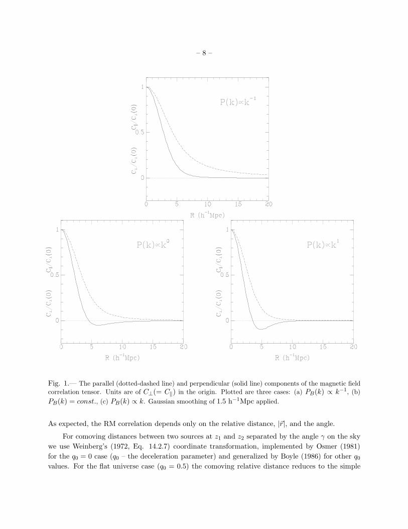
“magnetic power spectrum”, PB(k). Figure 1 show the two functions C‖(r) and C⊥(r) in units

of C⊥(0) for three values of the power index n = −1, 0, 1 [PB(k) ∝ kn]. Each function is shown

with a minimal Gaussian smoothing of 1.5 h−1Mpc. Naturally, smaller power indices mean larger

correlation length.

Going back to the expression (10) for the RM correlation we can rewrite it as

Υ0 =

(e3nb0

2πm2e

)2 ∫ r1(z1)

0

dr′1√1−Kr

′21

(1 + z′1)3∫ r2(z2)

0

dr′2√1−Kr

′22

(1 + z′2)3×

[C‖(r

′)− C⊥(r′)](q1 · r′)(q2 · r′) + C⊥(r

′)q1 · q2. (15)

– 8 –

Fig. 1.— The parallel (dotted-dashed line) and perpendicular (solid line) components of the magnetic field

correlation tensor. Units are of C⊥(= C‖) in the origin. Plotted are three cases: (a) PB(k) ∝ k−1, (b)

PB(k) = const., (c) PB(k) ∝ k. Gaussian smoothing of 1.5 h−1Mpc applied.

As expected, the RM correlation depends only on the relative distance, |~r|, and the angle.

For comoving distances between two sources at z1 and z2 separated by the angle γ on the sky

we use Weinberg’s (1972, Eq. 14.2.7) coordinate transformation, implemented by Osmer (1981)

for the q0 = 0 case (q0 – the deceleration parameter) and generalized by Boyle (1986) for other q0values. For the flat universe case (q0 = 0.5) the comoving relative distance reduces to the simple

– 9 –

form

r(z1, z2, γ) =1

H0

[r1(z1)

2 + r2(z2)2 − 2r1(z1)r2(z2) cos γ

]1/2. (16)

The distance to a source at the redshift z (no cosmological constant) is given by (Kolb & Turner

1990, Eq. 3.112)

r(z) =1

H0

2Ω0z + (2Ω0 − 4)(√Ω0z + 1− 1)

Ω20(1 + z)

, (17)

and can be easily generalized for other cases.

In order to estimate the importance of Υξ [Eq. (12)] we adopt the APM power spectrum

(Baugh & Efstathiou 1993; Tadros & Efstathiou 1995) with the fitting formula

Pm(k) =2π2

k3(k/k0)

3−m

1 + (k/kc)−(m+n), (18)

the fitting parameters m = 1.4, kc = 0.02, k0 = 0.19, and Gaussian smoothing of 1.5 h−1Mpc.

We then derive the real space correlation function by the Fourier transform of the smoothed power

spectrum. In the range 3 − 30 h−1Mpc the result is very similar to the derived APM real space

correlation function (no explicit smoothing) ξ0 = (r/5.25 h−1Mpc)−1.7 (Baugh 1995). For this

choice we get (regardless of the PB(k) form, and for zsrc >∼ 0.5), |Υξ/Υ| < 10−4. We hence identify

Υ = Υ0 hereafter.

2.1. The Power Spectrum Normalization

We relate the magnetic field normalization to the power spectrum by Brms(R) where

(BG,THrms )2(R) =

3

2π2

∫ ∞

0PB(k)k

2W 2G,TH(kR)dk , (19)

the factor 3 is due to the definition of PB(k) [as C⊥(r)], and WG,TH(kR) is the Gaussian (Top-hat)

window function of radius R, in k space,

WG = exp

[−(kR)2

2

]; WTH =

3

(kR)3[sin(kR)− kR cos(kR)] . (20)

A good benchmark to use for the normalization range is the CMB limit due to its simplicity and

the availability of ∆T/T measurements on many scales (either today or in the near future). We

therefore work in the range of ∼ 1 nG throughout this paper.

The observational limits on the magnetic field as deduced from the RM dipole [R ≃ r(z = 2.5)

or R ≃ r(z = 3.6)] are thus very different from the limits imposed by CMB fluctuations on 1′ scale.

We note that by Eq. (19) one cannot infer limits on the magnetic field magnitude from one scale

to another. The limits must involve the power spectrum shape. Since no estimate for the latter

exists, and since theoretical predictions for it range from power index of n = −3 to n = 2 (Ratra

1992a), limits on one particular scale hardly limit other scales.

– 10 –

Fig. 2.— RM correlation as function of the separation angle between source pairs at three different redshifts.The redshift values are zsrc = 0.5, 1, 2 with thicker lines for higher redshift. The magnetic field normalization

in all cases is BTHrms(50 h−1Mpc) = 1 nG . Three magnetic power spectra are shown with the power indices

n = −1, 0, 1. Note the different y axis scales.

Figure 2 show the values for the RM correlation function for pairs of sources at the same

redshift, and three different spectral indices. The normalization of the magnetic field in each case

is BTHrms(50 h−1Mpc) = 1 nG (Ωm = 1, h = 1,Ωb = 0.024). This scale resembles the mean separation

between rich clusters.

We notice that for close pairs, high redshift sources are preferable in order to get high signal,

while a transition typically occurs at a fraction of a degree where it becomes preferable to use lower

redshift sources. This transition is due to the uncorrelated magnetic fields experienced by high

redshift sources with large separation. Only when the two lines-of-sight approach the correlation

length, does contribution to the RM correlation becomes substantial. The different, uncorrelated

– 11 –

magnetic fields up to the correlation length, play the role of uncorrelated noise, and dominate the

correlated signal from the low redshift segment of the line-of-sight.

On the scale 0.5−2.5, the RM correlation signal still stands on ∼ 10−102 rad2m−4 depending

on the power spectrum.

3. CALCULATION PROCEDURE FOR THE CORRELATION MATRIX

3.1. The Raw Data

The raw data consist of Nsrc extra Galactic objects for which polarization measurements are

available in Nλ wavelengths. Broten, Macleod, & Vallee (1988), and Oren & Wolfe (1995) have

emphasized the need for a careful selection of wavelengths for each observed source. For the

current application there are additional special requirements that will become clear when we get

to the discussion (§5).Each of such Nλ measurements consists of two types of data : the degree of polarization, and the

polarization position angle [|p| and 2φ of Eq. (3)]. Two functions are then constructed which give

the dependence of these on wavelength. The RM is computed from the latter by using Eq. (3) where

RM = φλ−2. Each measured RMm value has an error, ǫm, that emerges from the measurement

error (instrumental, ionosphere model, the earth magnetic field model etc.) and translates to the

error in the fit from which the RM is derived. For typical sources with polarization degree of>∼ 10% (namely 10−1 − 10−2 Jy of polarized component at a few GHz frequency), the measurement

error in each datum is of the order of a few degrees (e.g. Kato, Tabara, Inoue & Aizu 1987;

Simard-Normandin, Kronberg, Button, 1980 (SKB); Oren & Wolfe 1995). For realistic Nλ = 4,

this instrumental error translates to a typical error in the φ−λ2 fit of 0.5−5 radm−2 and is dwarfed

by other noise terms in the procedure (cf. §3.2, §3.3). We therefore set ǫm ≃ 0 from now on.

The measured RMs are the sum of a few contributions, and cannot be directly plugged into

the expression (15) to evaluate Υ.

To begin with, there exists the internal RMI for every one of the Nsrc extragalactic sources. Then

there is the integrated RMc which is presumably due to the cosmological magnetic field (and

the free electrons) along the line-of-sight to the source. There may also exist contribution RMf

from intervening systems along the line-of-sight (foreground screen) either next to the source itself

(e.g. the host galaxy of a quasar), Lyman-α systems, galaxies, or clusters of galaxies. Before this

combined signal gets to the detector it still has to go through the Galactic magnetic field, where it

is rotated once more by the amount RMG. The final measurement, RMm is thus the linear sum

RMm(~zi) = RMiI +RMc(~zi) + RMf (~zi) + RMG(zi) , (21)

where ~zi is the redshift-vector [actually translated to a distance vector (cf. §2)] for the ith source.

Since we are interested in the cosmological contribution to the RM [i.e. the second term in Eq. (21)],

the first step should involve “cleaning” the measured signal of all irrelevant extra contributions.

We shall attempt to perform this cleaning in a statistical way.

– 12 –

3.2. The Galactic Mask

There are two alternatives to assess the Galactic contribution to the measured RM. The two

ways differ by the population sample used for the assessment. If an independent population at

the outskirts of the Galaxy exists, for which RM can be measured, this population can be used to

map out the Galactic RM. We shall hereafter use the term “mask source population” for the set

of objects by which we map the Galactic contribution to the RM.

An estimate for the thickness of the Galactic magnetic layer is ∼ 1 kpc (Simard-Normandin

& Kronberg 1980). That means that apart from the Galactic center direction, sources of distances

that satisfy rsrc > 1/ sin(|b|) kpc (∼ 3 kpc for |b| = 20) are located beyond the Reynolds layer and

fully probe the Galactic contribution to the RM. We hence consider two possibilities for the mask

source population.

One natural candidate for this role is the pulsar population, for which RMs are available. In

order to make use of the pulsars we need to find a subset of them that reside in the outer part of

the Milky-way magnetic layer.

A class of pulsars that is especially appropriate for the task of probing the Galactic RM contribution

is the millisecond pulsars. This population of old pulsars is believed to reside far out of the Galactic

plane. The number density of millisecond pulsars as implied by a number of surveys at high Galactic

latitude (∼ 1mJy sensitivity at ∼ 1 GHz) ranges between 0.01−0.0175 deg−2, i.e. 400−700 pulsars

over the sky (Foster, Cadwell, Wolszczan, & Anderson 1995; Camilo, Nice, & Taylor 1996).

The alternative mask population for assessment of the Galactic RM contribution is a sub-set

of the closest extragalactic sources. The disadvantage of using this population is the need for a

large enough source number at low enough redshift, to allow differentiation between the cosmological

contribution and the Galactic one. Exploiting extragalactic sources for the resolution of the Galactic

contribution affects only slightly the amount of cosmological contribution correlation, as long as

the nearby sources are taken within z <∼ 0.1, since the bulk of the sources is at z >∼ 1 (cf. §4).In order to use either one of the galactic mask populations, its number density should exceed

a certain minimal number density. We now attempt to assess this minimal number.

The Galactic RM contribution is a two-dimensional field with RM values. The data on the other

hand are made of distinctive sources located at discrete directions. The lines-of-sight to the Galac-

tic mask population, do not necessarily coincide with the line-of-sight direction towards the extra-

galactic sources. The way to circumvent this difficulty is by introducing a smoothed version of the

Galactic RM map, namely the field RMG(z). The two fields are connected via the smoothing angle

θs, and by a specific choice of a Gaussian smoothing for NG measurements of the Galactic RMG(zi)

located at the directions zi

RMG(z) =

NG∑i=1

RMiG exp

[− (zi−z)2

2θs

]

NG∑i=1

exp[− (zi−z)2

2θ2s

] . (22)

– 13 –

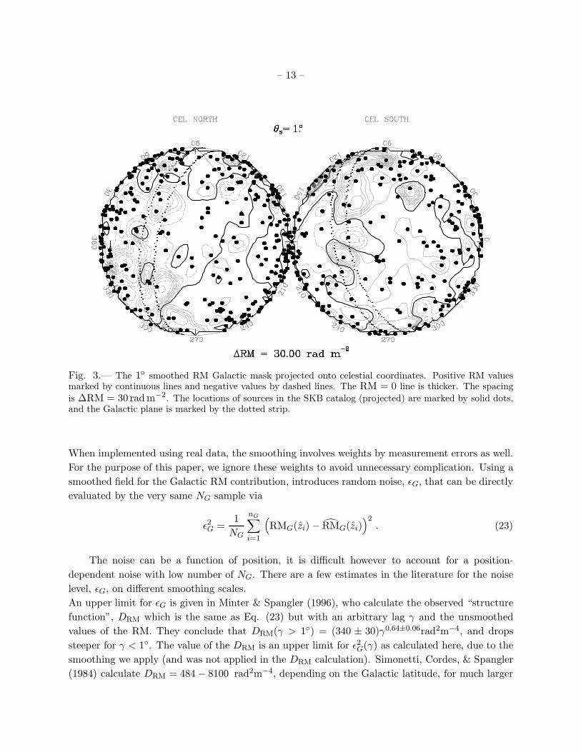
Fig. 3.— The 1 smoothed RM Galactic mask projected onto celestial coordinates. Positive RM valuesmarked by continuous lines and negative values by dashed lines. The RM = 0 line is thicker. The spacing

is ∆RM = 30 radm−2. The locations of sources in the SKB catalog (projected) are marked by solid dots,and the Galactic plane is marked by the dotted strip.

When implemented using real data, the smoothing involves weights by measurement errors as well.

For the purpose of this paper, we ignore these weights to avoid unnecessary complication. Using a

smoothed field for the Galactic RM contribution, introduces random noise, ǫG, that can be directly

evaluated by the very same NG sample via

ǫ2G =1

NG

nG∑

i=1

(RMG(zi)− RMG(zi)

)2. (23)

The noise can be a function of position, it is difficult however to account for a position-

dependent noise with low number of NG. There are a few estimates in the literature for the noise

level, ǫG, on different smoothing scales.

An upper limit for ǫG is given in Minter & Spangler (1996), who calculate the observed “structure

function”, DRM which is the same as Eq. (23) but with an arbitrary lag γ and the unsmoothed

values of the RM. They conclude that DRM(γ > 1) = (340 ± 30)γ0.64±0.06rad2m−4, and drops

steeper for γ < 1. The value of the DRM is an upper limit for ǫ2G(γ) as calculated here, due to the

smoothing we apply (and was not applied in the DRM calculation). Simonetti, Cordes, & Spangler

(1984) calculate DRM = 484 − 8100 rad2m−4, depending on the Galactic latitude, for much larger

– 14 –

Fig. 4.— The RM residuals from the 1 smoothed Galactic mask as function of the Galactic longitude (left)and latitude (right).

Fig. 5.— The 1 smoothed RM residuals of the Galactic mask in celestial coordinates. Symbols as in figure(3).

angular scales of 30 − 50 ! (linear scale).

Simonetti & Cordes (1986) corroborate these results and consider even larger angular scales to

obtain typically DRM < 1000 rad2m−4 on scales less than 100.

– 15 –

Oren & Wolfe (1995) calculate a very similar quantity to ǫG (with a varying top hat window instead

of a fixed Gaussian), and obtain a typical variance of < 1000 rad2m−4 on ∼ 30 scales.

All of these measurements suggest that for a mask population with number density of about one

source per 1000 deg.2 , the Galactic contribution to the RM (|b| > 20) can be resolved with a 1σ

accuracy of 30 radm−2. That means that an isotropic coverage of about 100 − 200 mask sources

on the sky is enough for achieving this noise level.

“Damage control” for ignoring the position dependence can be devised by comparing the “clean”

RM field dipole and quadrupole to the Galactic direction of the two. These first two multipole

should be the most prominent signature of the Galactic RM mask.

We go back to the suggested mask populations and examine whether they are able to fulfill

the requirement of the minimal number density.

The largest pulsar catalog to date [the electronic version of Taylor, Manchester, & Lyne (1993)]

consists of 800 pulsars out of which 259 have RM measurements. This catalog was not compiled

with a specific emphasis for millisecond pulsars, and therefore only 124 pulsars with RM values

lie in Galactic latitude |b| > 5. The softer condition rsrc > 2/ sin(|b|) (i.e. considering an “RM

layer” of 4 kpc) is fulfilled for 237 pulsars with both RM registered value and estimated distance

rsrc (Taylor & Cordes 1993).

However, these 237 pulsars are still not distributed isotropically across the sky, and tend to con-

centrate near the Galactic plane.

A way to avoid this anisotropy is to compile a sample of millisecond pulsars, that lie far away

from the Galactic plane. This population has a number density that exceeds the necessary ∼ 10−2

deg.−2 by at least a factor of two and it may be as high as seven times denser than the minimal

value. This population can be detected for RM (Fernando Camilo, private communication, 1997)2 and ensures the ǫG ≃ 30 radm−2 noise level. This kind of sample is ideal for the current paper

analysis, as it does not contain any cosmological contribution or internal RM contribution. The

main disadvantage of it is that it does not exist yet.

In considering the extragalactic mask population; for the <∼ 400 sources needed to resolve the

Galactic contribution, it is sufficient to have a sample of 1mJy sensitivity (at a few GHz) up to

z ≃ 0.1 [see Loan, Wall, & Lahav (1997) for the number density of radio sources with flux > 35

mJy, and Dunlop & Peacock (1990) for the combined flat/steep spectrum luminosity function for

extrapolation to the 1mJy limit].

For this paper we follow Oren & Wolfe (1995) and use an extragalactic sample of RM measure-

ments as an upper limit for the noise that appears by the Galactic RM removal procedure. The

sample we use consists of 555 sources as listed by SKB. The SKB catalog allows us to realistically

mimic the Galactic mask, and is an overestimate since we ascribe all the RM of the sources to the

Galactic contribution. Moreover, unlike Oren & Wolfe we do not exclude “outliers”. This use aims

2In the Taylor, Manchester, & Lyne catalog there are two pulsars with both RM registered value and p < 10 ms,

and five for which p < 100 ms. The smallest polarized flux at 1.4GHz for a pulsar with a registered RM is 0.2mJy

– 16 –

to provide a realistic model of the Galactic mask contribution, and allows us to demonstrate the

method power. For our purpose it should not be taken literally as the true Galactic mask contribu-

tion (even though Oren & Wolfe did consider it that way) because no segregation by redshift was

applied to choose mask sources from the SKB list. We neither attempted to evaluate the internal

RM (by means explained in §3.3) in order to minimize the ǫG value.

The SKB source locations (projected, and therefore concentrated toward the circumference)

are marked as black dots on Figure 3 and shown on top of the smoothed Galactic RM field with

smoothing scale of θs = 1. The smooth map is shown in celestial coordinates. Figure 4 shows the

RM residuals as functions of Galactic latitude and longitude, and figure 5 shows the contour map

of the smoothed residual field. Both figures (4 & 5) show hardly any longitude dependence of the

residuals (in spite of the solar system off-center position), and bigger residuals in the ∼ ±20 strip

about the Galactic plane (cf. the same conclusion of Oren & Wolfe 1995). In an all-sky coverage

of sources, this residual deviation should be of some worry, but as we shall see (§4.2), it doesn’t

bias the result for the most likely power spectrum as calculated by the Bayesian analysis. If the

analysis is confined to high latitudes, then no systematic error due to the Galactic mask is expected

(cf. §4). For a few square degrees area, we notice there are typically no significant gradients in

the Galactic RM field beyond |b| >∼ 30. This allows us to use the smooth value safely when

analyzing a small area with extragalactic RM measurements. This value is also consistent with all

the abovementioned values of DRM as obtained by more detailed analyses.

3.3. The Internal Variation and foreground screens

We would like to get an estimate for the internal RM contribution and for the foreground

screen contribution (if the latter exists). We do not attempt to correct each individual source for

the RM contribution due to the internal and foreground screen terms. We do not take the measured

RM and subtract an estimate for RMI+f , we rather attempt to estimate the distribution of RMI+f ,

and treat it as another noise term.

The difference between the two separate terms in Eq. (21) (RMI and RMf ) emerges from

the fact that while the internal contribution is obtained from the same medium that emits the

polarized light, the foreground screen only serves as a filter for an already existing signal. In

previous investigations, attempts were made to separate the two contributions (Burn 1966; Laing

1984), later on it became clear that the signature of the two is rather similar (Tribble 1991).

For our purposes we are interested in all previous calculations’ “left overs”, their signal is

our noise and vice versa. For the noise estimate we claim it is legitimate to take the internal

contribution and the foreground screen contribution together. We argue that the two can be dealt

with simultaneously. To this end we shall use the other piece of information provided by the

observations – the polarization degree.

Tribble (1991) shows the connection between the observed depolarization (as a function of

– 17 –

wavelength) and the observed RM for an extended source. Using this connection, and provided

the polarization measurements are available, a direct estimate for the internal RM can be carried

out. Recall we do not expect any depolarization due to the cosmological RM since the cosmological

coherence we are after is orders of magnitude bigger (>∼ a few h−1Mpc) than the source size.

It is interesting to note, that even if we had perfect information about the depolarization

due to the source structure and foreground screen contribution and an exact relation between the

depolarization degree and the RM, we could still not subtract this derived RM from the observed

one. This is due to the fact that the polarization degree doesn’t specify the RM direction.

Tribble’s statistical connection between the observed depolarization and the observed RM is

valid only if the correlation scale of the RM structure function for the source or the foreground

screen is much shorter than the telescope beam size. This condition is probably not valid for

individual damped Lyman–α systems, and galaxies that serve as foreground screens, and for which

long range correlation across the telescope beam may exist.

Full justification for neglecting damped Lyman–α systems and galaxies exists only if we can

avoid lines-of-sight that cross such systems. Otherwise the order of magnitude of an intervening

galaxy contribution is obtained as follows: For a galaxy seen face-on, where there is a danger of a

well ordered magnetic field, the disc thickness, to which the magnetic field is presumably connected

is of the order of kpc (Simard-Normandin & Kronberg 1980). Observations show magnetic field

magnitude of ∼ µG, mainly in the disc plane. In order to equate this to a cosmological magnetic

field of the order of nG, and coherent scale of 50 h−1Mpc, the average baryon number density across

the galaxy should be at least fifty times higher than the cosmological nb.

However, we do not expect any correlation between the magnetic field orientation of galaxies

along the line-of-sight, or galaxies adjacent (in angle) to each other. The worst contribution to

the RM, could only come from a random walk of Nf steps where Nf is the number of foreground

screens (intervening systems) along the line-of-sight. Since one can model the probability for an

intersecting system along the line-of-sight as a function of the source redshift (Welter, Perry, &

Kronberg 1984; Lanzetta, Wolfe, & Turnshek 1995), another noise term can be added. We did not

attempt to model this noise term here, because we believe that the best strategy would be to avoid

highly contributing (i.e. damped Lyman-α and Lyman limit) intervening systems. Low column

density Lyman-α system contribute very little to the RM signal (see Eq. (1.2) in Welter, Perry, &

Kronberg 1984). An exception may exist, if two sources (or two separated parts of the same source)

cross the same cluster. In that case the noise of the two sources (RMI+f ) may be correlated, but

then we can go back to the technique that uses the depolarization, in an attempt to remove the

noise correlation.

The best strategy, as stated earlier, would be to avoid intervening systems altogether. There

are two methods for doing this. The first method is simply to avoid intervening systems by looking

for sources that exhibit no absorption lines in their spectra (we assume spectrography is carried

out anyway, to allow redshift determination). The existence of a large fraction of quasar lines-of-

sight which do not intersect a dense intervenor is corroborated by Møller & Jakobsen (1990) and

– 18 –

Lanzetta, Wolfe, & Turnshek (1995) analyses.

The other method is to put a depolarization limit on the observations (e.g. the one imposed

by Tabara & Inoue 1979). Such a limit naturally reduces the noise term of ǫI+f and does not affect

the correlation signal. As a matter of fact, a sequence of such depolarization limits, may be helpful

in constituting the estimate for ǫI+f . There are yet more methods for minimizing the number of

sources that manifest internal RM as we shall point out when we consider real observations (§5).

3.4. Bayesian Likelihood Analysis

In the current stage of research we have very little knowledge about the power spectrum of the

cosmological magnetic field. We can hardly even put limits on its integral value, i.e. the rms value

of the field. There are, however predictions regarding the power spectrum shape and amplitude. In

the lack of any observational preference towards any of these predictions (apart from the limits on

its rms value), we assume that all models are equally probable. Conventional estimates of the RM

correlation, estimates of the sort applied to galaxies are not very useful. It is difficult to get correct

error estimate without simulations, that in turn must assume some magnetic field power spectrum,

moreover in the traditional correlation calculation procedure, the errors of different bins in r space

are correlated. On top of that, the quantity we are after is the magnetic field power spectrum,

and the inversion from the integrated RM back to the magnetic field is a non-trivial one. All of

the above lead us to the use of Bayesian statistics as a tool for finding the best parameters, and

their probability, given a model. In the Bayesian formalism, the a-posteriori probability density of

a model, m, given the data, d, is

P(m|d) = P(m)P(d|m)

P(d). (24)

As stated earlier, P(m), the model probability density is unknown and therefore assumed uniform

for all models. The data probability, in the denominator is the same for all models, and therefore

serves as a normalization factor. We are thus left with equivalence between the operation of

maximizing the probability of the model, given the data [P(m|d)] and the operation of maximizing

the probability of the data, given the model [P(d|m)]. This equivalence allows us to write down

the likelihood function for Nsrc sources with measured RM.

We begin by constructing the Nsrc ×Nsrc symmetric matrix Υij of the expectation values for

the RM correlation (Eq. 15) between these sources (as determined by their position). We further

assume that the errors in each RM value are uncorrelated and Gaussianly distributed. The variance

of the overall error is the sum of the quadratures of the various error sources i.e.

ǫ2i = ǫ2G + ǫ2I+f,i + ǫ2m,i , (25)

and the likelihood function becomes

L = [(2π)Nsrc det(Υij)]−1/2 exp

−1

2

Nsrc∑

i,j

RMiΥ−1ij RMj

, (26)

– 19 –

where Υij = Υij + δKij ǫ2i .

The χ2 statistic is defined as χ2 = −2lnL. The χ2 statistics as defined, is a χ2 distribution (of

Nsrc degrees of freedom) with respect to the data points, not the model parameters. This χ2 is

interpreted as a rough estimate for the confidence levels in the parameter space.

3.5. Estimating the Signal-to-Noise Ratio

Before proceeding to the elaborated description of the various tests we performed with artificial

data, we would like to get a rough estimate for the expected RM correlation and the necessary

number of sources for a high enough signal-to-noise ratio at various scales. We temporarily abandon

the Bayesian approach, and focus on P(m|d). Recall that the noise in the cross correlation is not

correlated, but may still dominate the signal if not appropriately averaged over many pairs. The

signal-to-noise ratio for an individual measurement of a pair at identical redshift, a separation angle

γ, and in the context of a specific model, is given by

⟨Υ(z, γ)

ǫ2

⟩=

〈Υ(z, γ)〉〈ǫ2〉 , (27)

where in the last equality we assume no dependence between the various noise terms and the model

(cosmology + power spectrum). The cosmological parameters we choose to use are as follows: We

restrict ourselves to flat cosmology with Ωm = 1, we choose H0 = 100 km s−1Mpc−1 (but the

scaling with h is straightforward). We take the ionization factor to be Xn = 1 which according

to the Gunn-Peterson effect (Gunn & Peterson 1965) is a reasonable choice, and Ωb = 0.024h−2

(Tytler, Fan, & Burles 1996), i.e. nb = 2.6× 10−7 cm−3.

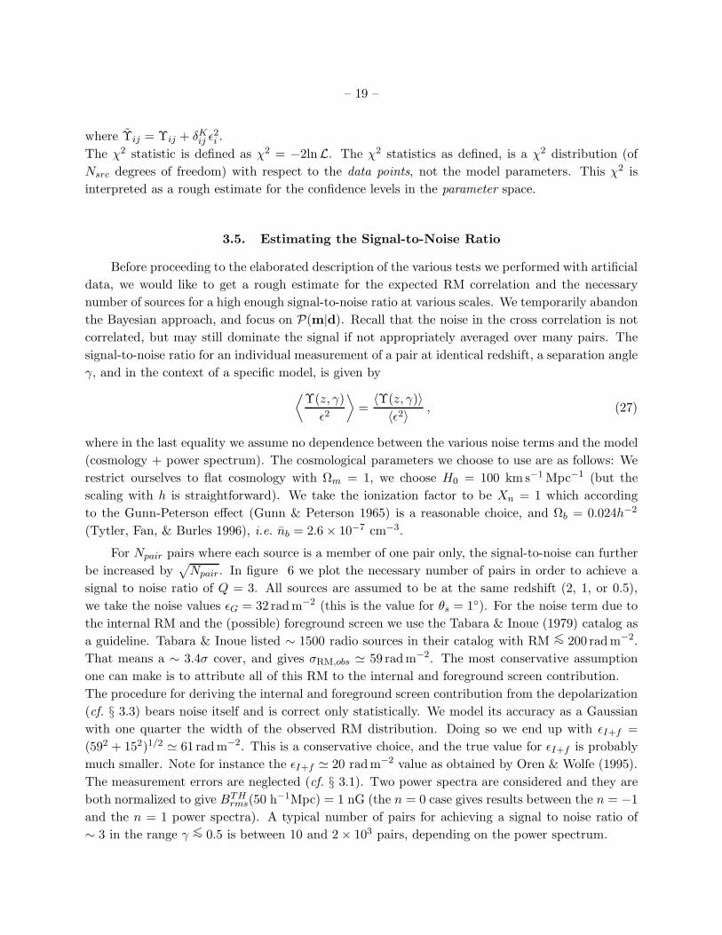
For Npair pairs where each source is a member of one pair only, the signal-to-noise can further

be increased by√Npair. In figure 6 we plot the necessary number of pairs in order to achieve a

signal to noise ratio of Q = 3. All sources are assumed to be at the same redshift (2, 1, or 0.5),

we take the noise values ǫG = 32 radm−2 (this is the value for θs = 1). For the noise term due to

the internal RM and the (possible) foreground screen we use the Tabara & Inoue (1979) catalog as

a guideline. Tabara & Inoue listed ∼ 1500 radio sources in their catalog with RM <∼ 200 radm−2.

That means a ∼ 3.4σ cover, and gives σRM,obs ≃ 59 radm−2. The most conservative assumption

one can make is to attribute all of this RM to the internal and foreground screen contribution.

The procedure for deriving the internal and foreground screen contribution from the depolarization

(cf. § 3.3) bears noise itself and is correct only statistically. We model its accuracy as a Gaussian

with one quarter the width of the observed RM distribution. Doing so we end up with ǫI+f =

(592 + 152)1/2 ≃ 61 radm−2. This is a conservative choice, and the true value for ǫI+f is probably

much smaller. Note for instance the ǫI+f ≃ 20 radm−2 value as obtained by Oren & Wolfe (1995).

The measurement errors are neglected (cf. § 3.1). Two power spectra are considered and they are

both normalized to give BTHrms(50 h−1Mpc) = 1 nG (the n = 0 case gives results between the n = −1

and the n = 1 power spectra). A typical number of pairs for achieving a signal to noise ratio of

∼ 3 in the range γ <∼ 0.5 is between 10 and 2× 103 pairs, depending on the power spectrum.

– 20 –

Fig. 6.— Estimate of the number of pairs at separation γ needed to achieve signal to noise ratio of 3. Themagnetic field is normalized by BTH

rms(50 h−1Mpc) = 1 nG, and the noise calculation is explained in thetext. Two cases for power index of −1 (left) and 1 (right) are plotted.

This estimate of Q is not accurate. To begin with, for Nsrc sources we expect less than

(N2src −Nsrc)/2 statistically independent pairs. We do not expect all sources to reside at the same

redshift, neither do we expect the errors to be identical for all sources. Furthermore, the separation

between the sources is not fixed , but rather is spread from the arc-minute scale to 180. Due

to the need for a realistic error estimate, and a demonstration of an actual implementation of the

technique we propose, led us to apply it to mock catalogs, for which the underlying power spectrum

is known.

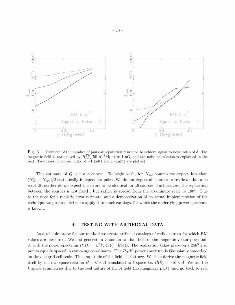
4. TESTING WITH ARTIFICIAL DATA

As a reliable probe for our method we create artificial catalogs of radio sources for which RM

values are measured. We first generate a Gaussian random field of the magnetic vector potential,~A with the power spectrum PA(k) = k2PB(k)(= E(k)). The realization takes place on a 2563 grid

points equally spaced in comoving coordinates. The PB(k) power spectrum is Gaussianly smoothed

on the one grid cell scale. The amplitude of the field is arbitrary. We then derive the magnetic field

itself by the real space relation ~B = ~∇× ~A translated to k space i.e. ~B(~k) = −i~k × ~A. We use the

k space symmetries due to the real nature of the ~A field (no imaginary part), and go back to real

– 21 –

space to obtain a divergence-free magnetic field with the desired correlation function, and periodic

boundary conditions. We check the resultant field by calculating the field divergence about each

and every grid point in real space and get ~∇ · ~B/Brms < 5× 10−5.

At this point we select the cosmology into which we embed the simulation. Our standard

choice is identical to the one described in the signal-to-noise estimate (§ 3.5). Due to the limited

dynamical range, we choose the grid scale to represent 1.5 h−1Mpc, and we are therefore confined

to a largest simulation wavelength of 768 h−1Mpc.

We then select the source mask, i.e. the source distribution across the sky, and their redshifts.

The two-dimensional distribution is taken to be a Poisson-like distribution, this choice allows us

to have close pairs (unlike grid selection), but to be as conservative as possible in terms of the

angular correlation function of the sources. Introducing any correlation as observed for radio

sources (Kooiman, Burne & Klypin 1995; Sicotte 1995; Cress et al. 1995; Loan, Wall, & Lahav

1997) can only increase the number of close pairs on small angles, and thus improve the RM

correlation resultant signal (see fig. 6). We do not take explicitly into account very small angle

(sub arc-minute) separations that may exist in real data sets for resolved extended sources, whose

different parts can be used as more than one background source. We employ two distribution

schemes, an all-sky coverage, and a cover of 150 deg.2 area centered about the north Galactic pole.

The source redshift distribution is selected according to the N(z) of radio sources with flux

> 35 mJy (at 4.85 GHz) as calculated by Loan, Wall, & Lahav (1997) who used the mean of

the theoretical luminosity function models of Dunlop & Peacock (1990) and kindly provided their

fit. Loan et al. (1997) N(z) is peaked around z = 1, and has a shape resembling a low redshift

truncated Gaussian of width (2 × σ) ∆z ≃ 1.9.

In principle, setting flux limit and sky coverage, sets the source number. In practice only a

sub-set of all radio sources emit polarized light. A random sample taken from the NVSS survey

(Condon et al. 1994) shows registered polarization angle for ∼ 40% of the sources. Refraining from

sources with intervening systems and large internal RM may further decrease the number. Since

the source number density in the radio catalogs of this flux limit is a few per square degree, when

we prepare an “all-sky” coverage catalog (see below), we are always way below the available number

of sources. For smaller angular coverage with higher source density, one has to further decrease

the flux limit. For example in the 2.5 mJy limit we expect ∼ 50 sources per square degree (NVSS,

Condon et al. 1994), and in the 1 mJy limit we expect source density of about 100 per square

degree (the “FIRST” survey; Becker, White, & Helfand 1995).

The N(z) function of Loan et al. (1997) is therefore interpreted as a normalized selection

function, with a cutoff at the highest redshift of the catalog. We expect this selection function to

provide an underestimate for the number of sources at high redshift, if a lower flux limit is set.

Since sources at higher redshift typically bear higher signal (without changing the noise), such an

imposed selection is a conservative choice in terms of the expected signal-to-noise ratio 3.

3The N(z) we choose, which is peaked in a relatively low redshift, may be useful in mimicking another effect. As

– 22 –

For each selected source, we integrate along the line-of-sight over the dot product between

the magnetic field and the line-of-sight direction using the periodic boundary conditions. The

integration scheme assigns weights to each integration segment, k, according to

wBk =

(1 + zk)3

√1−Kr2k(zk)

, (28)

in order to account for the cosmological evolution.

We then add the following noise terms to the resultant RM

1. Internal variation + foreground screens.

We draw this noise term from a Gaussian of (59 radm−2)2 variance (cf. § 3.5). This is the

added RM to the cosmological one. However, we also try to imitate the procedure of ǫI+f

evaluation by the depolarization. To this end, for a specific value of RMiI+f (drawn earlier),

we mimic the recovery of the ǫI+f from the depolarization degree, by listing an ǫI+f value

scattered about RMiI+f . The scatter has a Gaussian distribution of (15 radm−2)2 variance.

This is the error in the noise estimate. The “observer” takes into account the scattered value

of the ǫI+f and not the value that was actually added to the integrated cosmological RM.

2. Galactic mask.

We use the model-estimate of the Galactic mask, smoothed to 1 scale (see § 3.2). Since the

smoothed galactic RM differs from the true RM to the line-of-sight, we add a RM drawn from

a Gaussian distribution with the standard deviation of ǫG = 32 radm−2 (Eq. 23).

At the end of this process we are left with a mock RM catalog that consists of source coordinates

and redshift, measured RM value, and the total error in the RM value (i.e. ǫI+f ).

We proceed by feeding the mock catalog into the maximum likelihood procedure. In the

current application, we consider only the right cosmology, i.e. the one in which the simulation was

embedded. In principle the sensitivity to the cosmology choice can be checked as well. The two

variables for the model are the amplitude and the power index. It is really the combination of the

two that the likelihood procedure constraints best.

The statistical significance of the χ2 distribution (as defined following Eq. (26)) is obtained in the

standard way. The number of degrees of freedom is the source number minus the number of fitting

parameters, and the goodness of fit is calculated by taking into account the value of χ2min. If the

goodness of fit turns out to be very small (< 0.1), this is a clear indication for convergence to the

wrong minimum, and vice versa. For the right solution the minimum value for the χ2 per degree

of freedom (the source number) is typically unity within 10−3 accuracy.

the source redshift increases, the probability for intervening systems along the line-of-sight increases as well. If in a

sample compilation we try to avoid intervening system, this attempt translates to a steeper fall-off of the selection

function.

– 23 –

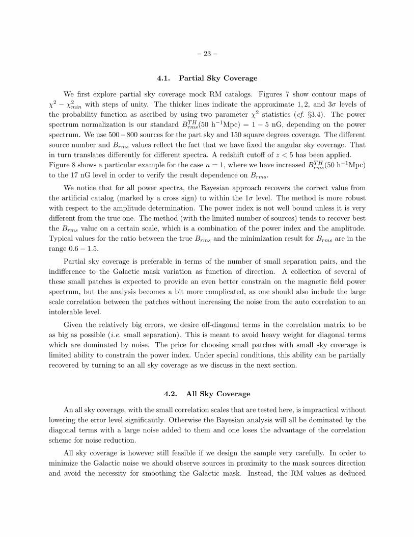
4.1. Partial Sky Coverage

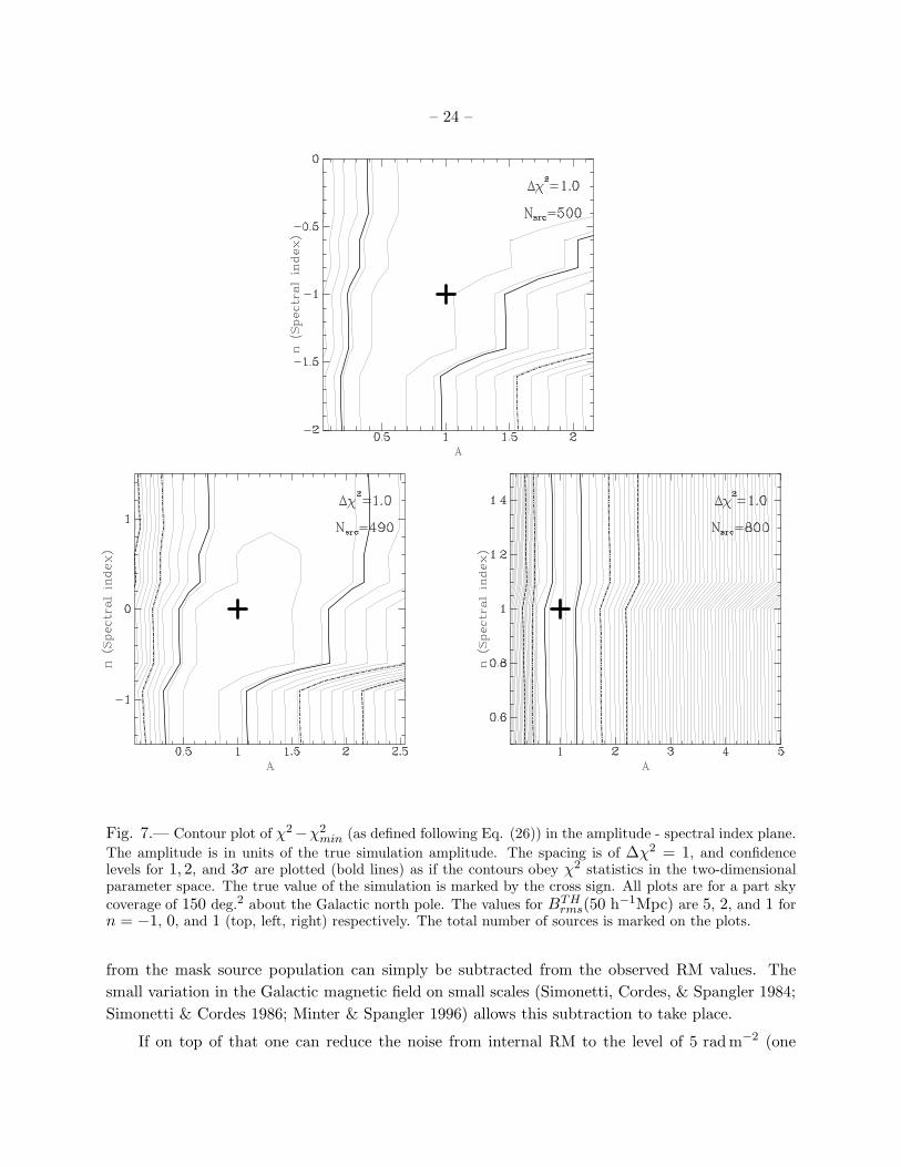
We first explore partial sky coverage mock RM catalogs. Figures 7 show contour maps of

χ2 − χ2min with steps of unity. The thicker lines indicate the approximate 1, 2, and 3σ levels of

the probability function as ascribed by using two parameter χ2 statistics (cf. §3.4). The power

spectrum normalization is our standard BTHrms(50 h−1Mpc) = 1 − 5 nG, depending on the power

spectrum. We use 500−800 sources for the part sky and 150 square degrees coverage. The different

source number and Brms values reflect the fact that we have fixed the angular sky coverage. That

in turn translates differently for different spectra. A redshift cutoff of z < 5 has been applied.

Figure 8 shows a particular example for the case n = 1, where we have increased BTHrms(50 h−1Mpc)

to the 17 nG level in order to verify the result dependence on Brms.

We notice that for all power spectra, the Bayesian approach recovers the correct value from

the artificial catalog (marked by a cross sign) to within the 1σ level. The method is more robust

with respect to the amplitude determination. The power index is not well bound unless it is very

different from the true one. The method (with the limited number of sources) tends to recover best

the Brms value on a certain scale, which is a combination of the power index and the amplitude.

Typical values for the ratio between the true Brms and the minimization result for Brms are in the

range 0.6− 1.5.

Partial sky coverage is preferable in terms of the number of small separation pairs, and the

indifference to the Galactic mask variation as function of direction. A collection of several of

these small patches is expected to provide an even better constrain on the magnetic field power

spectrum, but the analysis becomes a bit more complicated, as one should also include the large

scale correlation between the patches without increasing the noise from the auto correlation to an

intolerable level.

Given the relatively big errors, we desire off-diagonal terms in the correlation matrix to be

as big as possible (i.e. small separation). This is meant to avoid heavy weight for diagonal terms

which are dominated by noise. The price for choosing small patches with small sky coverage is

limited ability to constrain the power index. Under special conditions, this ability can be partially

recovered by turning to an all sky coverage as we discuss in the next section.

4.2. All Sky Coverage

An all sky coverage, with the small correlation scales that are tested here, is impractical without

lowering the error level significantly. Otherwise the Bayesian analysis will all be dominated by the

diagonal terms with a large noise added to them and one loses the advantage of the correlation

scheme for noise reduction.

All sky coverage is however still feasible if we design the sample very carefully. In order to

minimize the Galactic noise we should observe sources in proximity to the mask sources direction

and avoid the necessity for smoothing the Galactic mask. Instead, the RM values as deduced

– 24 –

Fig. 7.— Contour plot of χ2−χ2min (as defined following Eq. (26)) in the amplitude - spectral index plane.

The amplitude is in units of the true simulation amplitude. The spacing is of ∆χ2 = 1, and confidencelevels for 1, 2, and 3σ are plotted (bold lines) as if the contours obey χ2 statistics in the two-dimensionalparameter space. The true value of the simulation is marked by the cross sign. All plots are for a part skycoverage of 150 deg.2 about the Galactic north pole. The values for BTH

rms(50 h−1Mpc) are 5, 2, and 1 forn = −1, 0, and 1 (top, left, right) respectively. The total number of sources is marked on the plots.

from the mask source population can simply be subtracted from the observed RM values. The

small variation in the Galactic magnetic field on small scales (Simonetti, Cordes, & Spangler 1984;

Simonetti & Cordes 1986; Minter & Spangler 1996) allows this subtraction to take place.

If on top of that one can reduce the noise from internal RM to the level of 5 radm−2 (one

– 25 –

Fig. 8.— Same as the n = 0 panel in the previous figure (fig. 7). Here BTHrms(50 h−1Mpc) is 17 nG, and

allows a better determination of the parameters.

can always avoid foreground screens) by multi wavelength observations, then it becomes sensible

to exploit an all-sky coverage.

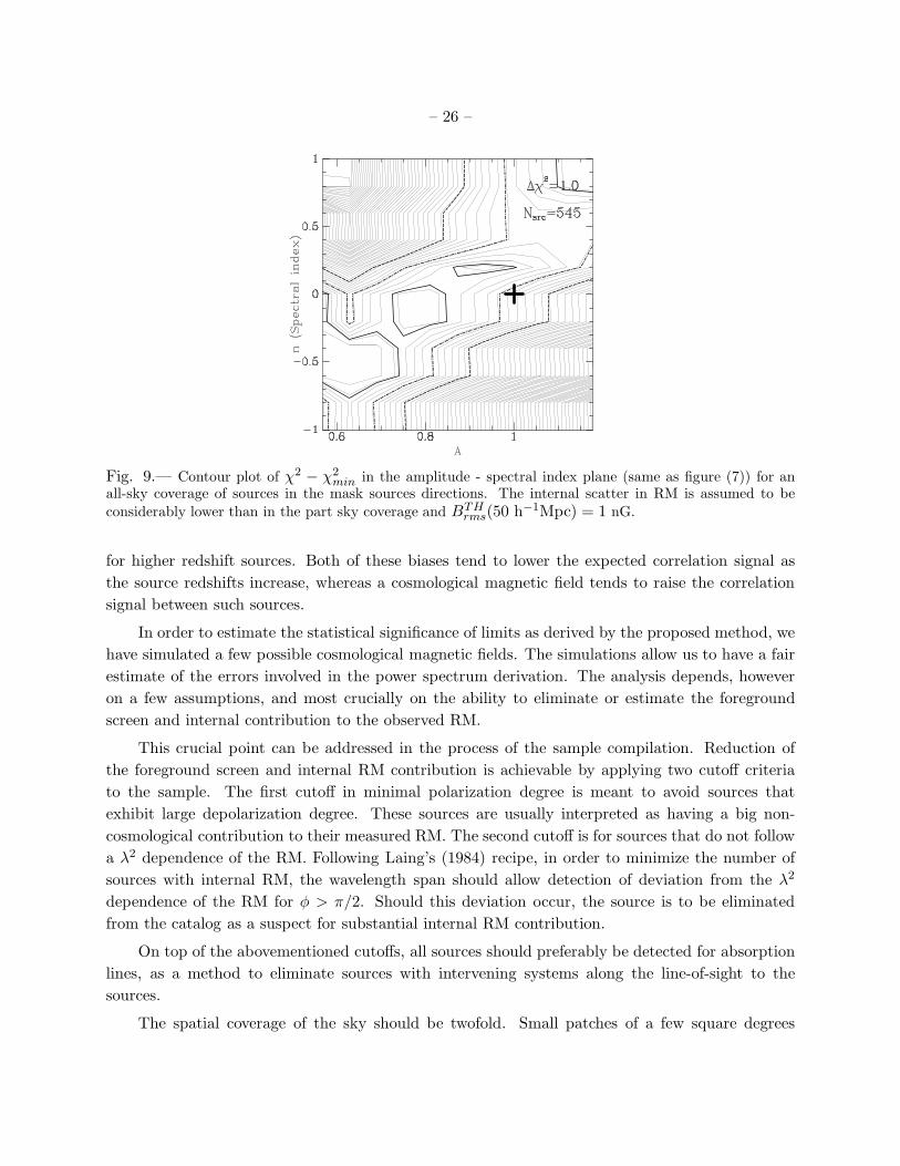
Figure 9 shows an example of a sample taken at the mask source directions with ǫI = 5 radm−2

and BTHrms(50 h−1Mpc) = 1 nG. The rest of the parameters are identical to those of the part

sky coverage (n = 1) of the last section. We notice that the power index is somewhat better

constrained in an all sky coverage, especially if the amplitude (or Brms) are assumed or known

from some different source. The true values are recovered to within the ∼ 2σ level. Moreover

such coverage allows us to calculate all prevailing magnetic fields on the sample scale, expressed as

PB(k) = δD(k − πR ) with δD the Dirac delta function and R the sample depth. Notice, however

that using the formalism proposed in section 2, we cannot take into account power spectra that are

not functions of |k| alone so this test is a bit weaker than the dipole test.

5. DISCUSSION AND CONCLUSIONS

We have presented the formalism for the RM correlation function and demonstrated that by

using it we can put limits on the power spectrum of the cosmological magnetic field. These limits

are more stringent than limits obtained by any other method that currently exists. Limits of 2−3σ

level for magnetic field of ∼ 1 nG on inter-cluster scales (∼ 50 h−1Mpc) can be devised with only

102 − 103 sources. The increment of the source number reflects linearly in the Brms limits.

We performed the statistical analysis following a Bayesian approach that seems to be the most

adequate for this problem. The correlation method we propose is also less susceptible to systematic

effects such as observational bias (or bias due to evolution) toward smaller internal RM measures

– 26 –

Fig. 9.— Contour plot of χ2 − χ2min in the amplitude - spectral index plane (same as figure (7)) for an

all-sky coverage of sources in the mask sources directions. The internal scatter in RM is assumed to beconsiderably lower than in the part sky coverage and BTH

rms(50 h−1Mpc) = 1 nG.

for higher redshift sources. Both of these biases tend to lower the expected correlation signal as

the source redshifts increase, whereas a cosmological magnetic field tends to raise the correlation

signal between such sources.

In order to estimate the statistical significance of limits as derived by the proposed method, we

have simulated a few possible cosmological magnetic fields. The simulations allow us to have a fair

estimate of the errors involved in the power spectrum derivation. The analysis depends, however

on a few assumptions, and most crucially on the ability to eliminate or estimate the foreground

screen and internal contribution to the observed RM.

This crucial point can be addressed in the process of the sample compilation. Reduction of

the foreground screen and internal RM contribution is achievable by applying two cutoff criteria

to the sample. The first cutoff in minimal polarization degree is meant to avoid sources that

exhibit large depolarization degree. These sources are usually interpreted as having a big non-

cosmological contribution to their measured RM. The second cutoff is for sources that do not follow

a λ2 dependence of the RM. Following Laing’s (1984) recipe, in order to minimize the number of

sources with internal RM, the wavelength span should allow detection of deviation from the λ2

dependence of the RM for φ > π/2. Should this deviation occur, the source is to be eliminated

from the catalog as a suspect for substantial internal RM contribution.

On top of the abovementioned cutoffs, all sources should preferably be detected for absorption

lines, as a method to eliminate sources with intervening systems along the line-of-sight to the

sources.

The spatial coverage of the sky should be twofold. Small patches of a few square degrees

– 27 –

enable the small separation pair number needed for noise reduction. Small patches, however, can

not reveal large correlation scales in an effective way. It is thus desirable to compile a dilute all sky

coverage sample, in addition to the high number density patches off the Galactic plane. The two

sampling strategies cover a large range of potential correlation scales, without the necessity for an

all-sky dense sample. The all sky coverage should preferably look for sources in proximity to the

mask sources directions in order to minimize the Galactic noise term. Accurate internal RM for

these sources should be evaluated through depolarization measurements in order for them to be

useful for the power spectrum evaluation. Ultimately, the sample can always be mimicked in terms

of the exact source locations in the framework of all and every detected model. Exact imitation of

the source locations ensures the right correlation terms in the correlation matrix.

The limits we have derived here are a combination of limits on the free electron average density,

ne, and the magnetic field. If by any other fashion (like HII absorption) an estimate for ne can

be achieved, then the limits on B will become more robust. The estimate is also a function of the

assumed cosmology, and may be entangled with magnetic field evolution in the post recombination

era. We haven’t modeled such evolution in this paper.

This method of RM correlation can further be generalized to the smoothed RM correlation.

The data can be smoothed on a certain angular scale, and then either compared to the expectation

value predicted by a model, or inverted numerically to give limits on B. The Bayesian approach,

though ceases to be advantageous in the smoothed case, because even though the noise terms

decrease, the smoothing introduces correlation among the errors, and the statistical interpretation

becomes more hazardous.

A nice feature of the proposed analysis is that it is bound to yield results. These can be either

limits on the magnetic field magnitude, or actual detection of its value. Either way, these results

may help in lifting the curtain over the mystery of the cluster and galactic magnetic fields origin.

I would like to thank Arthur Kosowsky for extensive discussions and helpful assistance, George

Blumenthal for valuable insight and critical reading of the manuscript, and James Bullock for a

very carefull examination of the manuscript.

This work was supported in part by the US National Science Foundation (PHY-9507695).

REFERENCES

Adams, J., Danielsson, U.H., Grasso, D., & Rubinstein, H. 1996, sissa preprint, astro-ph/9607043

Barrow, J.D., Ferreira, P.G., & Silk, J. 1997, sissa preprint, astro-ph/9701063

Baugh, C.M. 1995, sissa preprint, astro-ph/9512011

Baugh, C.M. and Efstathiou, G. 1993, MNRAS, 265, 145

Becker, R.H., White, R.L., & Helfand, D.J. 1995, ApJ, 450, 559

Boyle, B.J. 1986, PhD thesis, University of Durham

– 28 –

Brandenburg, A., Enquist, K., & Olesen, P. 1996, sissa preprint, asrto-ph/9602031

Broten, N.W., Macleod, J.M., & Vallee, J,P. 1988, Ap&SS, 141, 303

Burn, B.J. 1966, MNRAS, 133, 67

Camilo, F., Nice, D.J., & Taylor J.H. 1996, ApJ, 461, 812

Cheng, B.L., Olinto, A.V., Schramm, D.N., & Truran, J.W 1996, Phys. Rev. D, 54, 4714

Condon, J.J., Cotton, W.D., Greisen, E.W., Yin, Q.F., Perley, R.A., & Broderick, J.J. 1994, in

Astronomical Data Analysis Software and Systems III, A.S.P. Conference Series, Vol. 61

Eds. Dennis, R. Crabtree, R.J., Barnes H., & Barnes, J. p. 155

Cress, C.M., Helfand, D.J., Becker, R.H., Gregg, M.D., White, R.L. 1996, ApJ, 473, 7

Dolgov, A. & Silk, J. 1993 Phys. Rev. D, 47, 3144

Dunlop, J.S. & Peacock, J.A. 1990 MNRAS, 247, 19

Foster, R.S., Cadwell, B.J., Wolszczan, A., & Anderson, S.B. 1995, ApJ, 454, 826

Grasso, D. & Rubinstein H.R. 1995, Nucl. Phys. B, 43, 303

Grasso, D. & Rubinstein H.R. 1996, Phys. Let. B, 388, 253

Gunn, J.E. & Peterson, B.,A. 1965, ApJ, 142, 1633

Harrison, E.R. 1973, Phys. Rev. Lett., 30, 18

Kato, T., Tabara, H., Inoue, M., & Aizu, K. 1987, Nature, 329, 223

Kolb, E.W. & Turner, M.S. 1990, The Early Universe, (USA: Addison-Wesley) p. 84

Kooiman, B.L., Burns, J.O., & Klypin, A.A. 1995, ApJ, 448, 500

Kronberg, P.P. 1976, Int. Astron. Union Symp. 74, 367

Kronberg, P.P. 1994, Rep. Prog. Phys., 57, 325 (K94)

Kronberg, P.P. & Simard-Normandin, M. 1976, Nature, 263, 653

Laing, R.A. 1984, in Physics of Energy Transport in Extragalactic Radio Sources, edited by Bridle,

A.H. & Eilek, J.A. (Green Bank W.Va. USA:NRAO) p. 90

Lang, K.R. 1978, Astrophysical Formulae, (New-York: Springer-Verlag) p. 57

Lanzetta, K.M., Wolfe, A.M., Turnshek, D.A. 1995, ApJ, 440, 425

Lee, S., Olinto, A.V., & Sigl, G. 1995, ApJ, 455, L21

Loan, A.J., Wall, J.V., & Lahav, O. 1997, MNRAS, 286, 994

Loeb, A. & Kosowsky, A. 1996, ApJ, 469, 1

Masden, M.S. 1989, MNRAS, 237, 109

Minter, A.H. & Spangler, S.R. 1996, ApJ, 458, 194

Møller, P. & Jakobsen, P. 1990, A&A228, 299

– 29 –

Monin, A.S. & Yaglom, A.M. 1975, Statistical Fluid Mechanics (Cambridge; MIT Press), pp. 29–52

Nissen, D. & Thielheim, K.O. 1975, Ap&SS, 33, 441

Oren, A.L. & Wolfe, A.M. 1995 ApJ, 445, 624

Osmer, P.S. 1981, ApJ, 247, 762

Ostriker, J.P. & Thompson, C. 1987, ApJ, 323, L97

Parker, E.N. 1979, Cosmical Magnetic Fields (Oxford; Clarendon Press) p. 616

Pudritz, R.E. & Silk, J. 1989, ApJ, 342, 650

Quashnock, J.M., Loeb, A., & Spergel, D.N. 1989, ApJ, 342, 650

Ratra, B. 1992a, Phys. Rev. D, 45, 1913

Ratra, B. 1992b, ApJ, 391, L1

Rees, M.,J. 1987, QJRAS, 28, 197

Sicotte, H., 1995, Ph.D. thesis, Princeton University

Simard-Normandin, M. & Kronberg, P.P. 1980, ApJ, 242, 74

Simard-Normandin, M. & Kronberg, P.P., & Button, S. 1980, ApJS, 45, 97 (SKB)

Simonetti, J.H., Cordes, J.M., & Spangler, S.R. 1984 ApJ, 284, 126

Simonetti, J.H. & Cordes, J.M. 1986 ApJ, 310, 160

Tabara, H. & Inoue, M. 1979, A&ASupp., 39, 379

Tadros, H. & Efstathiou, G. 1995, MNRAS, 276, 45

Tajima, T., Cable, S., Shibata, K., & Kulsrud, R.M. 1992, ApJ, 390, 309

Taylor, J.H. & Cordes, J.M. 1993, ApJ, 411, 674

Taylor, J.H., Manchester, R.N., & Lyne, A.G. 1993, ApJS, 88, 529

Thompson, C. 1990, Int. Astron. Union Symp., 140, 127

Tribble, P.C. 1991, MNRAS, 250, 726

Turner, M.S. & Widrow, L.M. 1988, Phys. Rev. D, 37, 10

Tytler, D., Fan, X., & Burles, S. 1996, Nature, 381, 207

Vachaspati, T. 1991, Phys. Lett., 265, 258

Vallee, J.,P. 1990, ApJ, 360, 1

Waxman, E. & Miralda-Escude, J. 1996, ApJ, 472, L89

Weinberg, S. 1972, Gravitation and Cosmology (Wiley & Sons, NY) p. 413

Welter, G.L., Perry, J.J., & Kronberg, P.P. 1984, ApJ, 279, 19

Zel’dovich, Y.B. & Novikov, I.D., 1975, Relativistic Astrophysics, (Chicago; University of Chicago

Press)

– 30 –

Zweibel, E.G. 1988, ApJ, 329, L1

This preprint was prepared with the AAS LATEX macros v4.0.