Embed Size (px)
Citation preview
ARTIN APPROXIMATION
HERWIG HAUSER, GUILLAUME ROND
Abstract. In 1968, M. Artin proved that any formal power series solutionof a system of analytic equations may be approximated by convergent powerseries solutions. Motivated by this result and a similar result of Płoski, he con-jectured that this remains true when we replace the ring of convergent powerseries by a more general ring.This paper presents the state of the art on this problem, aimed at non-experts.In particular we put a slant on the Artin Approximation Problem with con-straints.
Contents
1. Introduction 12. Artin Approximation 142.1. The analytic case 142.2. Artin Approximation and Weierstrass Division Theorem 232.3. Néron’s desingularization and Popescu’s Theorem 253. Strong Artin Approximation 283.1. Greenberg’s Theorem: the case of a discrete valuation ring 283.2. Strong Artin Approximation Theorem: the general case 323.3. Ultraproducts and proofs of Strong Approximation type results 343.4. Effectivity of the behaviour of Artin functions: some examples 364. Examples of Applications 415. Approximation with constraints 435.1. Examples 435.2. Nested Approximation in the algebraic case 465.3. Nested Approximation in the analytic case 495.4. Other examples of approximation with constraints 55Appendix A. Weierstrass Preparation Theorem 58Appendix B. Regular morphisms and excellent rings 58Appendix C. Étale morphisms and Henselian rings 60References 63
1. Introduction
The aim of this paper is to present the Artin Approximation Theorem and somerelated results. The problem we are interested in is to find analytic solutions of somesystem of equations when this system admits formal power series solutions and theArtin Approximation Theorem yields a positive answer to this problem. We begin
Date: March 11, 2013.1
2 HERWIG HAUSER, GUILLAUME ROND
this paper by giving several examples explaining what this sentence means exactly.Then we will present the state of the art on this problem. There is essentially threeparts: the first part is dedicated to present the Artin Approximation Theorem andits generalizations; the second part presents a stronger version of Artin Approxima-tion Theorem; the last part is mainly devoted to explore the Artin ApproximationProblem in the case of constraints. An appendix presents the algebraic materialused in this paper (Weierstrass Preparation Theorem, excellent rings, étales mor-phisms and Henselian rings).We do not give the proofs of all the results presented in this paper but, at least, wealways try to outline the proofs and give the main arguments.
Example 1. Let us consider the following curve C := {(t3, t4, t5), t ∈ C} in C3.This curve is an algebraic set which means that it is the zero locus of polynomialsin three variables. Indeed, we can check that C is the zero locus of the polynomialsf := y2 − xz, g := yz − x3 and h := z2 − x2y. If we consider the zero locus of anytwo of these polynomials we always get a set larger than C. The complex dimensionof the zero locus of one non-constant polynomial in three variables is 2 (such a setis called a hypersurface of C3). Here C is the intersection of the zero locus of threehypersurfaces and not of two of them, but its complex dimension is 1.In fact we can see this phenomenon as follows: we call an algebraic relation betweenf , g and h any element of the kernel of the linear map ϕ : C[x, y, z]3 −→ C[x, y, z]defined by ϕ(a, b, c) := af + bg + ch. Obviously r1 := (g,−f, 0), r2 := (h, 0,−f)and r3 := (0, h,−g) ∈ Ker(ϕ). These are called the trivial relations between f , gand h. But in our case there is one more relation which is r0 := (z, y,−x) and r0cannot be written as a1r1 +a2r2 +a3r3 with a1, a2 and a3 ∈ C[x, y, z], which meansthat r0 is not in the sub-C[x, y, z]-module of C[x, y, z]3 generated by r1, r2 and r3.On the other hand we can prove that Ker(ϕ) is generated by r0, r1, r2 and r3.Let X be the common zero locus of f and g. If (x, y, z) ∈ X and x 6= 0, thenh = zf+yg
x = 0 thus (x, y, z) ∈ C. If (x, y, z) ∈ X and x = 0, then y = 0. Geometri-cally this means thatX is the union of C and the z-axis, i.e. the union of two curves.
Now let us denote by CJx, y, zK the ring of formal power series with coefficientsin C. We can also consider formal relations between f , g and h, that is elementsof the kernel of the map CJx, y, zK3 −→ CJx, y, zK induced by ϕ. Any elementof the form a0r0 + a1r1 + a2r2 + a3r3 is a formal relation as soon as a0, a1, a2,a3 ∈ CJx, y, zK.In fact any formal relation is of this form, i.e. the algebraic relation generate theformal and analytic relations. We can show this as follows: we can assign theweights 3 to x, 4 to y and 5 to z. In this case f , g, h are homogeneous polynomialsof weights 8, 9 and 10 and r0, r1, r2 and r3 are homogeneous relations of weights(5, 4, 3), (9, 8, 0), (10, 0, 8) and (0, 10, 9). If (a, b, c) ∈ CJx, y, zK3 is a formal relationthen we can write a =
∑∞i=0 ai, b =
∑∞i=0 bi and c =
∑∞i=0 ci where ai, bi and ci are
homogeneous polynomials of degree i with respect to the previous weights. Thensaying that af + bg + ch = 0 is equivalent to
aif + bi−1g + ci−2h = 0 ∀i ∈ N
with the assumption bi = ci = 0 for i < 0. Thus (a0, 0, 0), (a1, b0, 0) and any(ai, bi−1, ci−2), for 2 ≤ i, are in Ker(ϕ), thus are homogeneous combinations of r0,r1, r2 and r3. Hence (a, b, c) is a combination of r0, r1, r2 and r3 with coefficients
ARTIN APPROXIMATION 3
in CJx, y, zK.
Now we can investigate the same problem by replacing the ring of formal powerseries by C{x, y, z}, the ring of convergent power series with coefficients in C, i.e.
C{x, y, z} :=
∑i,j,k∈N
ai,j,kxiyjzk / ∃ρ > 0,
∑i,j,k
|ai,j,k|ρi+j+k <∞
We can also consider analytic relations between f , g and h, that is elements of thekernel of the map C{x, y, z}3 −→ C{x, y, z} induced by ϕ. From the formal casewe see that any analytic relation r is of the form a0r0 + a1r1 + a2r2 + a3r3 withai ∈ CJx, y, zK for 0 ≤ i ≤ 4. In fact we can prove that ai ∈ C{x, y, z} for 0 ≤ i ≤ 4.Let us remark that, saying that r = a0r0 + a1r1 + a2r2 + a3r3 is equivalent to saythat a0,..., a3 satisfy a system of three affine equations with analytic coefficients.This is the first example of the problem we are interested in: if we some equationswith analytic coefficients have formal solutions do they have analytic solutions?Artin Approximation Theorem yields an answer to this problem. Here is the firsttheorem proven by M. Artin in 1968:
Theorem 1.1 (Artin Approximation Theorem). [Ar68] Let f(x, y) be a vector ofconvergent power series over C in two sets of variables x and y. Assume given aformal power series solution y(x),
f(x, y(x)) = 0.
Then there exists, for any c ∈ N, a convergent power series solution y(x),
f(x, y(x)) = 0
which coincides with y(x) up to degree c,
y(x) ≡ y(x) modulo (x)c.
We can define a topology on CJxK by saying that two power series are close iftheir difference is in a high power of the maximal ideal (x). Thus we can reformulateTheorem 1.1 as: formal power series solutions of a system of analytic equations maybe approximated by convergent power series solutions.
Example 2. A special case of Theorem 1.1 and a generalization of Example 1occurs when f is linear in y, say f(x, y) =
∑fi(x)yi, where fi(x) is a vector of
convergent power series with r coordinates for any i. A solution y(x) of f(x, y) = 0is a relation between the fi(x). In this case the formal relations are linear combi-nations of analytic combinations with coefficients in CJxK. In term of commutativealgebra, this is expressed as the flatness of the ring of formal power series over thering of convergent powers series, a result which can be proven via the Artin-ReesLemma.It means that if y(x) is a formal solution of f(x, y) = 0, then there exist analytic so-lutions of f(x, y) = 0 denoted by yi(x), 1 ≤ i ≤ s, and formal power series b1(x),...,bs(x), such that y(x) =
∑i bi(x)yi(x). Thus, by replacing in the previous sum the
bi(x) by their truncation at order c, we obtain an analytic solution of f(x, y) = 0coinciding with y(c) up to degree c.If the fi(x)’s are vectors of polynomials then the formal relations are also linearcombinations of algebraic relations since the ring of formal power series is flat over
4 HERWIG HAUSER, GUILLAUME ROND
the ring of polynomials, and Theorem 1.1 remains true if f(x, y) is linear in y andC{x} is replaced by C[x].
Example 3. A slight generalization of the previous example is when f(x, y) is avector of polynomials in y of degree one with coefficients in C{x} (resp. C[x]), say
f(x, y) =
m∑i=1
fi(x)yi + b(x)
where the fi(x)’s and b(x) are vectors of convergent power series (resp. polynomi-als). Here x and y are multi-variables If y(x) is a formal power series solution off(x, y) = 0, then (y(x), 1) is a formal power series solution of g(x, y, z) = 0 where
g(x, y, z) :=
m∑i=1
fi(x)yi + b(x)z
and z is a single variable. Thus using the flatness of CJxK over C{x} (resp. C[x])(Example 2), we can approximate (y(x), 1) by a convergent power series (resp. poly-nomial) solution (y(x), z(x)) which coincides with (y(x), 1) up to degree c. In orderto obtain a solution of f(x, y) = 0 we would like to be able to divide y(x) by z(x)since y(x)z(x)−1 would be a solution of f(x, y) = 0 approximating y(x). We canremark that, if c ≥ 1, then z(0) = 1 thus z(x) is not the ideal (x). But C{x} is alocal ring. We call a local ring any ring A that has only one maximal ideal. This isequivalent to say that A is the disjoint union of one ideal (its only maximal ideal)and of the set of units in A. In particular z(x)−1 is invertible in C{x}, hence wecan approximate formal power series solutions of f(x, y) = 0 by convergent powerseries solutions.In the case (y(x), z(x)) is a polynomial solution of g(x, y, z) = 0, z(x) is not invert-ible in general in C[x] since it is not a local ring. For instance set
f(x, y) := (1− x)y − 1
where x and y are single variables. Then y(x) :=
∞∑n=0
xn =1
1− xis the only formal
power series solution of f(x, y) = 0, but y(x) is not a polynomial. Thus we cannotapproximate the roots of f in CJxK by roots of f in C[x].But instead of working in C[x] we can work in C[x](x) which is the ring of rationalfunctions whose denominator does not vanish at 0. This ring is a local ring. Sincez(0) 6= 0, then y(x)z(x)−1 is a vector of rational function of C[x](x). In particularany system of polynomial equations of degree one with coefficients in C[x] whichhas solutions in CJxK has solutions in C[x](x).
Example 4. The next example we are looking at is the following: set f ∈ A whereA = C[x] or C[x](x) or C{x}. When do there exist g, h ∈ A such that f = gh?First of all, we can take g = 1 and h = f or, more generally, g a unit in A andh = g−1f . These are trivial cases and thus we are looking for non units g and h.Of course, if there exist non units g and h in A such that f = gh, then f =(ug)(u−1h) for any unit u ∈ CJxK. But is the following true: let us assume thatthere exist g, h ∈ CJxK such that f = gh. Then do there exist non units g, h ∈ Asuch that f = gh ?Let us remark that this question is equivalent to the following: if A
(f) is an integral
domain, is CJxK(f)CJxK still an integral domain?
ARTIN APPROXIMATION 5
The answer to this question is no in general: set A := C[x, y] and set f :=x2 − y2(1 + y). Then f is irreducible as a polynomial since y2(1 + y) is not asquare in C[x, y]. But f = (x + y
√1 + y)(x − y
√1 + y) where
√1 + y is a formal
power series such that√
1 + y2
= 1 + y. Thus f is not irreducible in CJx, yK nor inC{x, y} but it is irreducible in C[x, y] or C[x, y](x,y).
In fact it is easy to see that x+y√
1 + y and x−y√
1 + y are power series which arealgebraic over C[x, y], i.e. they are roots of polynomials with coefficients in C[x, y].The set of such algebraic power series is a subring of CJx, yK and it is denoted byC〈x, y〉. In general if x is a multivariable the ring of algebraic power series C〈x〉 isthe following:
C〈x〉 := {f ∈ CJxK / ∃P (z) ∈ C[x][z], P (f) = 0} .
It is not difficult to prove that the ring of algebraic power series is a subring ofthe ring of convergent power series and is a local ring. In 1969, M. Artin provedan analogue of Theorem 2.1 for the rings of algebraic power series [Ar69]. Thusif f ∈ C〈x〉 (or C{x}) is irreducible then it remains irreducible in CJxK, this isa consequence of Artin Approximation Theorem. From this theorem we can alsodeduce that if f ∈ C〈x〉
I (or C{x}I ), for some ideal I, is irreducible, then it remains
irreducible in CJxKICJxK .
Example 5. Let us strengthen the previous question. Let us assume that thereexist g, h ∈ CJxK such that f = gh with f ∈ A with A = C〈x〉 or C{x}. Then doesthere exist a unit u ∈ CJxK such that ug ∈ A and u−1h ∈ A ?The answer to this question is positive if A = C〈x〉 or C{x}, this is a non trivialcorollary of Artin Approximation Theorem (see Corollary 4.4). But it is negativein general for C〈x〉
I or C{x}I if I is an ideal. The following example is due to S. Izumi
[Iz92]:Set A := C{x,y,z}
(y2−x3) . Set ϕ(z) :=∑∞n=0 n!zn (this is a divergent power series) and set
f := x+ yϕ(z), g := (x− yϕ(z))(1− xϕ(z)2)−1 ∈ CJx, y, zK.
Then we can check that x2 = f g modulo (y2 − x3). Now let us assume thatthere exists a unit u ∈ CJx, y, zK such that uf ∈ C{x, y, z} modulo (y2 − x3).Thus P := uf − (y2 − x3)h ∈ C{x, y, z} for some h ∈ CJx, y, zK. We can checkeasily that P (0, 0, 0) = 0 and ∂P
∂x (0, 0, 0) = u(0, 0, 0) 6= 0. Thus by the ImplicitFunction Theorem for analytic functions there exists ψ(y, z) ∈ C{y, z}, such thatP (ψ(y, z), y, z) = 0 and ψ(0, 0) = 0. This yields
ψ(y, z) + yϕ(z)− (y2 − ψ(y, z)3)h(ψ(y, z), y, z)u−1(ψ(y, z), y, z) = 0.
By substituting 0 for y we obtain ψ(0, z) + ψ(0, z)3k(z) = 0 for some power seriesk(z) ∈ CJzK. Since ψ(0, 0) = 0, this gives that ψ(0, z) = 0, thus ψ(y, z) = yθ(y, z)with θ(y, z) ∈ C{y, z}. Thus we obtain
θ(y, z) + ϕ(z)− (y − y2θ(y, z)3)h(ψ(y, z), y, z)u−1(ψ(y, z), y, z) = 0
and by substituting 0 for y, we see that ϕ(z) = θ(0, z) ∈ C{z} which is a contra-diction.
6 HERWIG HAUSER, GUILLAUME ROND
Thus x2 = f g modulo (y2 − x3) but there is no unit u ∈ CJx, y, zK such thatuf ∈ C{x, y, z} modulo (y2 − x3).
Example 6. A similar question is the following: if f ∈ A with A = C[x], C[x](x),C〈x〉 or C{x} and if there exist a non unit g ∈ CJxK and an integer m ∈ N suchthat gm = f , does there exist a non unit g ∈ A such that gm = f?A weaker question is the following: if A
(f) is reduced, isCJxK
(f)CJxK still reduced? Indeed,
if gm = f for some non unit g then CJxK(f)CJxK is not reduced. Thus, if the answer to
the second question is positive, then there exists a non unit g ∈ A and a unit u ∈ Asuch that ugk = f for some integer k.
As before, the answer to the first question is positive for A = C〈x〉 and A = C{x}by Artin Approximation Theorem.If A = C[x] or C[x](x), the answer to this question is negative. Indeed let us con-sider f = xm +xm+1. Then f = gm with g := x m
√1 + x but there is no g ∈ A such
that gm = f .
Nevertheless, the answer to the second question is positive in the cases A = C[x]or C[x](x). This deep result is due to D. Rees (see [H-S06] for instance).
Example 7. Using the same notation as in Example 4 we can ask a strongerquestion: set A = C〈x〉 or C{x} and let f be in A. If there exist g and h ∈ C[x],vanishing at 0, such that f = gh modulo a large power of the ideal (x), do thereexist g and h in A such that f = gh? By example 4 there is no hope, if g and hexist, to expect that g and h ∈ C[x].We have the following theorem:
Theorem 1.2 (Strong Artin Approximation Theorem). [Ar69] Let f(x, y) be avector of polynomials over C in two sets of variables x and y. Then there existsa function β : N −→ N, such that for any integer c and any given approximatesolution y(x) at order β(c),
f(x, y(x)) ≡ 0 modulo (x)β(c),
there exists an algebraic power series solution y(x),
f(x, y(x)) = 0
which coincides with y(x) up to degree c,
y(x) ≡ y(x) modulo (x)c.
In particular, if gh−f ≡ 0 modulo (x)β(1), where β is the function of the previoustheorem for the polynomial y1y2 − f , and if g(0) = h(0) = 0, then there exist nonunits g and h ∈ C〈x〉 such that gh− f = 0.A natural question is: given f ∈ C[x] how to compute β or, at least, β(1)? Thatis, up to what order do we have to check that the equation y1y2 − f = 0 hasan approximate solution in order to be sure that this equation as solutions? Forinstance, if f := x1x2 − xd3 then f is irreducible but x1x2 − f ≡ 0 modulo (x)d forany d ∈ N, so obviously β(1) really depends on f .In fact, in Theorem 1.2 M. Artin proved that β can be chosen independently of thedegree of the components of the the vector f(x, y). But it is still an open problemto find effective bounds on β (see Section 3.4).
ARTIN APPROXIMATION 7
Example 8 (Ideal Membership Problem). Set f1,...., fr ∈ CJxK where x = (x1, ..., xn).Let us denote by I the ideal of CJxK generated by f1,..., fr. If g is a power series,how can we detect that g ∈ I or g /∈ I? Since a power series is determined byits coefficients, saying that g ∈ I will depend in general on a infinite number ofconditions and it will not be possible to check that all these conditions are satisfiedin finite time. Another problem is to find canonical representatives of power seriesmodulo the ideal I that will help us to make computations in the quotient ring CJxK
I .
One way to solve these problems is the following. Let us consider the following orderon Nn: for all α, β ∈ Nn, we say that α ≤ β if (|α|, α1, ..., αn) ≤lex (|β|, β1, ..., βn)where |α| := α1 + · · ·+ αn and ≤lex is the lexicographic order. For instance
(1, 1, 1) ≤ (1, 2, 3) ≤ (2, 2, 2) ≤ (3, 2, 1) ≤ (2, 2, 3).
This order induces an order on the sets of monomials xα11 ...xαn
n : we say that xα ≤ xβif α ≤ β. Thus
x1x2x3 ≤ x1x22x33 ≤ x21x22x23 ≤ x31x22x3 ≤ x21x22x33.
If f :=∑α∈Nn fαx
α ∈ CJxK, the initial exponent of f with respect to the previousorder is
exp(f) := min{α ∈ Nn / fα 6= 0} = inf Supp(f)
where the support of f is Supp(f) := {α ∈ Nn / fα 6= 0}. The initial term of f isfexp(f)x
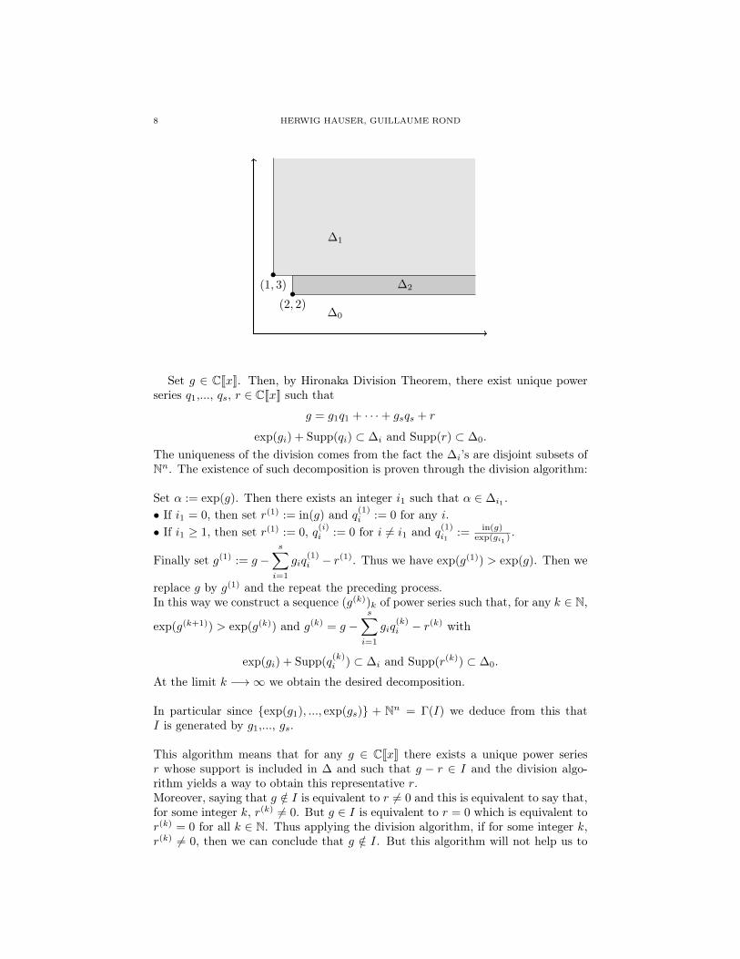
exp(f). This is the smallest non zero monomial in the Taylor expansion off with respect to the previous order.If I is an ideal of CJxK, we define Γ(I) to be the subset of Nn of all the initialexponents of elements of I. Since I is an ideal, for any β ∈ Nn and any f ∈ I,xβf ∈ I. This means that Γ(I) + Nn = Γ(I). Then we can prove that there existsa finite number of elements g1,..., gs ∈ I such that
{exp(g1), ..., exp(gs)}+ Nn = Γ(I).
Set
∆1 := exp(g1) + Nn and ∆i = (exp(gi) + Nn)\⋃
1≤j<i
∆j , for 2 ≤ i ≤ s.
Finally, set
∆0 := Nn\s⋃i=1
∆i.
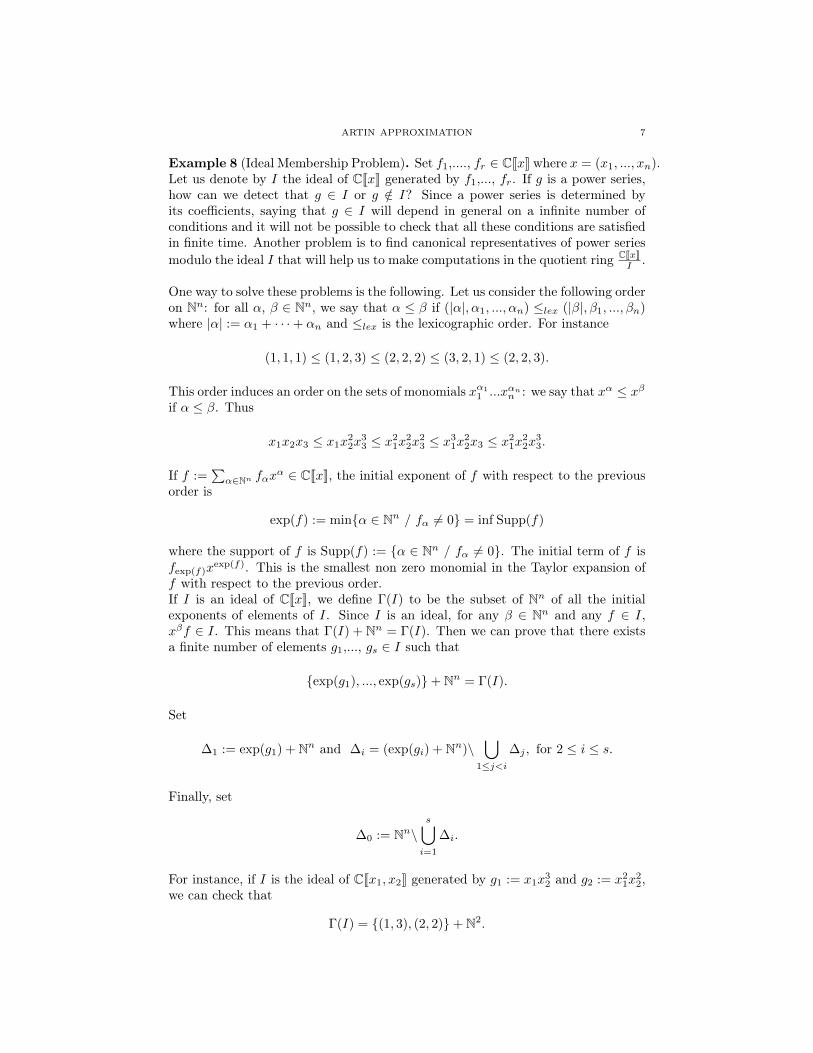
For instance, if I is the ideal of CJx1, x2K generated by g1 := x1x32 and g2 := x21x
22,
we can check that
Γ(I) = {(1, 3), (2, 2)}+ N2.
8 HERWIG HAUSER, GUILLAUME ROND
∆1
∆2
∆0
•(1, 3)
•(2, 2)
Set g ∈ CJxK. Then, by Hironaka Division Theorem, there exist unique powerseries q1,..., qs, r ∈ CJxK such that
g = g1q1 + · · ·+ gsqs + r
exp(gi) + Supp(qi) ⊂ ∆i and Supp(r) ⊂ ∆0.
The uniqueness of the division comes from the fact the ∆i’s are disjoint subsets ofNn. The existence of such decomposition is proven through the division algorithm:
Set α := exp(g). Then there exists an integer i1 such that α ∈ ∆i1 .• If i1 = 0, then set r(1) := in(g) and q(1)i := 0 for any i.• If i1 ≥ 1, then set r(1) := 0, q(i)i := 0 for i 6= i1 and q(1)i1 := in(g)
exp(gi1 ).
Finally set g(1) := g−s∑i=1
giq(1)i − r
(1). Thus we have exp(g(1)) > exp(g). Then we
replace g by g(1) and the repeat the preceding process.In this way we construct a sequence (g(k))k of power series such that, for any k ∈ N,
exp(g(k+1)) > exp(g(k)) and g(k) = g −s∑i=1
giq(k)i − r
(k) with
exp(gi) + Supp(q(k)i ) ⊂ ∆i and Supp(r(k)) ⊂ ∆0.
At the limit k −→∞ we obtain the desired decomposition.
In particular since {exp(g1), ..., exp(gs)} + Nn = Γ(I) we deduce from this thatI is generated by g1,..., gs.
This algorithm means that for any g ∈ CJxK there exists a unique power seriesr whose support is included in ∆ and such that g − r ∈ I and the division algo-rithm yields a way to obtain this representative r.Moreover, saying that g /∈ I is equivalent to r 6= 0 and this is equivalent to say that,for some integer k, r(k) 6= 0. But g ∈ I is equivalent to r = 0 which is equivalent tor(k) = 0 for all k ∈ N. Thus applying the division algorithm, if for some integer k,r(k) 6= 0, then we can conclude that g /∈ I. But this algorithm will not help us to
ARTIN APPROXIMATION 9
determine if g ∈ I since we would have to make a infinite number of computations.
Now a natural question is, what happens if we replace CJxK by A := C〈x〉 orC{x}? Of course we can proceed with the division algorithm but we do not know ifq1,..., qs, r ∈ A. In fact by controlling the size of the coefficients of q(k)1 ,..., q(k)s , r(k)at each step of the division algorithm, we can prove that if g ∈ C{x} then q1,...,qs and r remain in C{x} ([Hir64], [Gra72] and [dJ-Pf00]). But if g ∈ C〈x〉 then itmay happen that q1,..., qs and r are not in C〈x〉 (see Example 5.4 of Section 5).
Example 9 (Arcs Space and Jets Spaces). Let X be an affine algebraic sub-set of Cm, i.e. X is the zero locus of some polynomials in m variables: f1,...,fr ∈ C[y1, ..., ym]. Let t be a single variable. For any integer n, let us define Xn tobe the set of of vectors y(t) whose coordinates are polynomials of degree ≤ n andsuch that f(y(t)) ≡ 0 modulo (t)n+1. The elements of Xn are called n-jets on X.If yi(t) = yi,0 + yi,1t + · · · + yi,nt
n and if we consider each yi,j has one indetermi-nate, saying that f(y(t)) ∈ (t)n+1 is equivalent to the vanishing of rn polynomialsequations involving the yi,j ’s. This shows that the jets spaces of X are algebraicsets.For instance, if X is a cusp, i.e. the plane curve defined by X := {y21 − y32 = 0},then
X0 := {(a0, b0) ∈ C2 / a20 − b30 = 0} = X.
We have
X1 = {(a0, a1, b0, b1) ∈ C4 / (a0 + a1t)2 − (b0 + b1t)
3 ≡ 0 modulo t2}= {(a0, a1, b0, b1) ∈ C4 / a20 − b30 = 0 and 2a0a1 − 3b20b1 = 0}.
The morphisms C[t](t)k+1 −→ C[t]
(t)n+1 , for k ≥ n, induce truncation maps πkn : Xk −→Xn by reducing (k)-jets modulo (t)n+1. In the example we are considering, thefibre of π1
0 over the point (a0, a1) 6= (0, 0) is the line in the (a1, b1)-plane whoseequation is 2a0a1 − 3b20b1 = 0. This line is exactly the tangent space at X at thepoint (a0, b0). The tangent space at X in (0, 0) is the whole plane since this pointis a singular point of the plane curve X. This corresponds to the fact that the fibreof π1
0 over (0, 0) is the whole plane.On this example we show that X1 is isomorphic to the tangent bundle of X, whichis a general fact.We can easily see that X2 is given by the following equations:
a20 − b30 = 0
2a0a1 − 3b20b1 = 0
a21 + 2a0a2 − 3b0b21 − 3b20b2 = 0
In particular, the fibre of π20 over (0, 0) is the set of points of the form (0, 0, a2, 0, b1, b2)
and the image of this fibre by π21 is the line b1 = 0. This shows that π2
1 is not sur-jective.But, we can show that above the smooth part of X, the maps πn+1
n are surjectiveand the fibres are isomorphic to C.
The space of arcs on X, denoted by X∞, is the set of vectors y(t) whose coor-dinates are formal power series and such that f(y(t)) = 0. For such a generalvector of formal power series y(t), saying that f(y(t)) = 0 is equivalent to say that
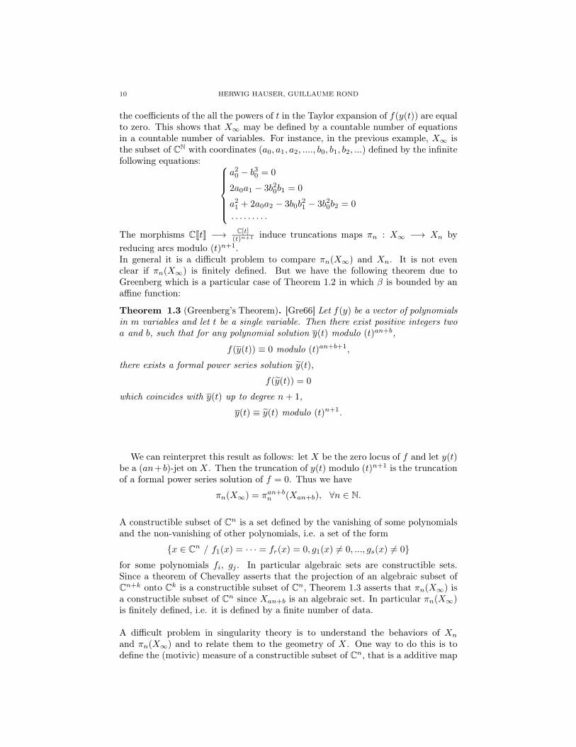
10 HERWIG HAUSER, GUILLAUME ROND
the coefficients of the all the powers of t in the Taylor expansion of f(y(t)) are equalto zero. This shows that X∞ may be defined by a countable number of equationsin a countable number of variables. For instance, in the previous example, X∞ isthe subset of CN with coordinates (a0, a1, a2, ...., b0, b1, b2, ...) defined by the infinitefollowing equations:
a20 − b30 = 0
2a0a1 − 3b20b1 = 0
a21 + 2a0a2 − 3b0b21 − 3b20b2 = 0
· · · · · · · · ·
The morphisms CJtK −→ C[t](t)n+1 induce truncations maps πn : X∞ −→ Xn by
reducing arcs modulo (t)n+1.In general it is a difficult problem to compare πn(X∞) and Xn. It is not evenclear if πn(X∞) is finitely defined. But we have the following theorem due toGreenberg which is a particular case of Theorem 1.2 in which β is bounded by anaffine function:
Theorem 1.3 (Greenberg’s Theorem). [Gre66] Let f(y) be a vector of polynomialsin m variables and let t be a single variable. Then there exist positive integers twoa and b, such that for any polynomial solution y(t) modulo (t)an+b,
f(y(t)) ≡ 0 modulo (t)an+b+1,
there exists a formal power series solution y(t),
f(y(t)) = 0
which coincides with y(t) up to degree n+ 1,
y(t) ≡ y(t) modulo (t)n+1.
We can reinterpret this result as follows: let X be the zero locus of f and let y(t)be a (an+b)-jet on X. Then the truncation of y(t) modulo (t)n+1 is the truncationof a formal power series solution of f = 0. Thus we have
πn(X∞) = πan+bn (Xan+b), ∀n ∈ N.
A constructible subset of Cn is a set defined by the vanishing of some polynomialsand the non-vanishing of other polynomials, i.e. a set of the form
{x ∈ Cn / f1(x) = · · · = fr(x) = 0, g1(x) 6= 0, ..., gs(x) 6= 0}for some polynomials fi, gj . In particular algebraic sets are constructible sets.Since a theorem of Chevalley asserts that the projection of an algebraic subset ofCn+k onto Ck is a constructible subset of Cn, Theorem 1.3 asserts that πn(X∞) isa constructible subset of Cn since Xan+b is an algebraic set. In particular πn(X∞)is finitely defined, i.e. it is defined by a finite number of data.
A difficult problem in singularity theory is to understand the behaviors of Xn
and πn(X∞) and to relate them to the geometry of X. One way to do this is todefine the (motivic) measure of a constructible subset of Cn, that is a additive map
ARTIN APPROXIMATION 11
χ from the set of constructible sets to a commutative ring R, such that:• χ(X) = χ(Y ) as soon as X and Y are isomorphic algebraic sets,• χ(X\U) + χ(U) = χ(X) as soon as U is an open set of an algebraic set X,• χ(X × Y ) = χ(X).χ(Y ) for any algebraic sets X and Y .Then we are interested in understand the following formal power series:∑
n∈Nϕ(Xn)Tn and
∑n∈N
χ(πn(X∞))Tn ∈ RJT K.
The reader may consult [De-Lo99], [Lo00], [Ve06] for instance.
Example 10. Let f1,..., fr ∈ k[x, y] where k is an algebraically closed field andx := (x1, ..., xn) and y := (y1, ..., ym) are multivariables. Moreover we will assumehere that k is uncountable. As in the previous example let us define the followingsets:
Xl := {y(x) ∈ k[x]m / fi(x, y(x)) ∈ (x)l+1 ∀i}.As we have done in the previous example, for any l there exists an integer N(l) ∈ Nsuch that Xl ⊂ kN(l). Moreover Xl is an algebraic subset of KN(l) and the mor-phisms k[x]
(x)k+1 −→ k[x](x)l+1 for k ≤ l induce truncations maps πkl : Xk −→ Xl for any
k ≥ l.
By a theorem of Chevalley, for any l ∈ N, the sequence (πkl (Xk))k is a decreasingsequence of constructible subsets ofXl. Thus the sequence (πkl (Xk))k is a decreasingsequence of algebraic subsets of Xl, where Y denotes the Zariski closure of a subsetY , i.e. the smallest algebraic set containing Y . By Noetherianity this sequencestabilizes: πkl (Xk) = πk
′l (Xk) for all k and k′ large enough (say for any k, k′ ≥ kl).
Let us denote by Fl this algebraic set.Let us assume that Xk 6= ∅ for any k ∈ N. This implies that Fl 6= ∅. Set
Ck,l := πkl (Xk). It is a constructible set whose Zariski closure is Fl for any k ≥ kl.Thus Ck,l has the form Fl\Vk where Vk is an algebraic proper subset of Fl, for anyk ≥ kl. Since k is uncountable the set Ul :=
⋂k Ck,l =
⋂k Fl\Vk is not empty. By
construction Ul is exactly the set of points of Xl that can be lifted to points of Xk
for any k ≥ l. In particlar πkl (Uk) = Ul. If x0 ∈ U0 then x0 may be lifted to U1,i.e. there exists x1 ∈ U1 such that π1
0(x1) = x0. By induction we may construct asequence of points xl ∈ Ul such that πl+1
l (xl+1) = xl for any l ∈ N. At the limit weobtain a point x∞ in X∞, i.e. a power series y(x) ∈ kJxKm solution of f(x, y) = 0.
We have proved here the following result similar to Theorem 1.2: if k is a un-countable algebraically closed field and if f(x, y) = 0 has solutions modulo (x)k forany k ∈ N, then there exists a power series solution y(x):
f(x, y(x)) = 0.
This kind of argument using asymptotic contructions (here the Noetherianity is thekey point of the proof) may be nicely formalized using ultraproducts. Ultraproductsmethods can be used to prove easily stronger results as Theorem 1.2 (See Part 3.3and Proposition 3.25).
Example 11 (Linearization of germ of diffeomorphism). Given f ∈ C{x}, x beinga single variable, let us assume that f ′(0) = λ 6= 0. Then f defines an analytic
12 HERWIG HAUSER, GUILLAUME ROND
diffeomorphism from a neighborhood of 0 in C onto a neighborhood of 0 in C pre-serving the origin. The linearization problem, firstly investigated by C. L. Siegel,is the following: is f conjugated to its linear part? That is: does there existg(x) ∈ C{x}, with g′(0) 6= 0, such that f(g(x)) = g(λx) or g−1 ◦ f ◦ g(x) = λx (inthis case we say that f is analytically linearizable)?This problem is difficult and the following cases may occur: f is not lineariz-able, f is formally linearizable but not analytically linearizable (i.e. g exists butg(x) ∈ CJxK\C{x}), f is analytically linearizable (see [Ce91]).
Let us assume that f is formally linearizable, i.e. there exists g(x) ∈ CJxK suchthat f(g(x))− g(λx) = 0. By considering the Taylor expansion of g(λx):
g(λx) = g(y) +
∞∑n=1
(y − λx)n
n!f (n)(y)
we see that there exists h(x, y) ∈ CJx, yK such that g(λx) = g(y) + (y − λx)h(x, y).Thus f is formally linearizable if and only if that there exists h(x, y) ∈ CJx, yK suchthat
f(g(x))− g(y) + (y − λx)h(x, y) = 0.
This former equation is equivalent to the existence of k(y) ∈ CJyK such that{f(g(x))− k(y) + (y − λx)h(x, y) = 0
k(y)− g(y) = 0
Using the same trick as before (Taylor expansion), this is equivalent to the existenceof l(x, y, z) ∈ CJx, y, zK such that
(1)
{f(g(x))− k(y) + (y − λx)h(x, y) = 0
k(y)− g(x) + (x− y)l(x, y) = 0
Hence, we see that, if f is formally linearizable, there exists a formal solution(g(x), k(z), h(x, y), l(x, y, z)) of the system (1). Such a solution is called a solutionwith constraints. On the other hand, if the system (1) has a convergent solution(g(x), k(z), h(x, y), l(x, y, z)), then f is analytically linearizable.
We see that the problem of linearizing analytically f when f is formally linearizableis equivalent to find convergent power series solutions of the system (1) with con-straints. Since it happens that f may be analytically linearizable but not formallylinearizable, such a system (1) may have formal solutions with constraints but noanalytic solutions with constraints.In Section 5 we will give some results about the Artin Approximation Problem withconstraints.
Example 12. Another related problem is the following: if a differential equationwith convergent power series coefficients has a formal power series solution, does ithave convergent power series solutions? We can ask the same question by replacing"convergent" by "algebraic".For instance let us consider the (divergent) formal power series y(x) :=
∑n≥0
n!xn+1.
ARTIN APPROXIMATION 13
It is straightforward to check that it is a solution of the equation
x2y′ − y + x = 0 (Euler Equation).
On the other hand if∑n anx
n is a solution of the Euler Equation then the sequence(an)n satisfies the following recursion:
a0 = 0, a1 = 1
an+1 = nan ∀n ≥ 1.
Thus an+1 = (n + 1)! for any n > 0 and y(x) is the only solution of the EulerEquation. Hence we have an example of a differential equation with polynomialscoefficients with a formal power series solution but without convergent power seriessolution. We will discuss in Section 5 how to relate this phenomenon to an ArtinApproximation problem for polynomial equations with constraints (see Example5.2).
14 HERWIG HAUSER, GUILLAUME ROND
Conventions We will assume that all the rings we consider are Noetheriancommutative rings with unit. Ring morphisms A −→ B are assumed to take theunit element of A into the unit element of B.If A is a local ring, then mA will denote its maximal ideal. For any f ∈ A, f 6= 0,
ord(f) := max{n ∈ N \ f ∈ mnA}.
If A is an integral domain, Frac(A) denotes its field of fractions.If no other indication is given the letters x and y will always denote multivariables,x := (x1, ..., xn) and y := (y1, ..., ym), and t will denote a single variable.If f(y) is a vector of polynomials with coefficients in a ring A,
f(y) := (f1(y), ..., fr(y)) ∈ A[y]r,
if I is an ideal of A and y ∈ Am, then f(y) ∈ I (resp. f(y) = 0) means fi(y) ∈ I(resp. fi(y) = 0) for 1 ≤ i ≤ r.
2. Artin Approximation
In this first part we review the main results concerning the Artin ApproximationProperty. We give four results that are the most characteristic in the story: theclassical Artin Approximation Theorem in the analytic case, its generalization by A.Płoski, a result of J. Denef and L. Lipschitz concerning rings with the WeierstrassDivision Property and, finally, Popescu’s Approximation Theorem.
2.1. The analytic case. In the analytic case, the first result is due to MichaelArtin in 1968 [Ar68]. His result asserts that the set of convergent solutions is densein the set of formal solutions of a system of implicit analytic equations. This resultis particularly useful, since if you have some analytic problem that you can expressin a system of analytic equations, in order to find solutions of this problem youonly need to find formal solutions and this may be done in general by an inductiveprocess. Another way to use this result is the following: let us assume that you havesome algebraic problem and that you are working over a ring of the form A := kJxK,where x := (x1, ..., xn) and k is a characteristic zero field. If the problem involvesonly a countable number of data (which is often the case in this context), sinceC is algebraically closed and the transcendence degree of Q −→ C is uncountable,you may assume that you work over CJxK. Using Theorem 2.1, you may, in somecases, reduce the problem to A = C{x}. Then you can use powerful methods ofcomplex analytic geometry to solve the problem. This kind of method is used, forinstance, in the proof of the Nash Conjecture for algebraic surfaces (see TheoremA of [FB12] and the crucial use of this theorem in [FB-PP1]) or in the proof of theAbhyankar-Jung Theorem given in [P-R12].Let us mention that C. Chevalley had apparently proven this theorem some yearsbefore M. Artin but he did not publish it because he did not find applications of it[Ra].
2.1.1. Artin’s result.
Theorem 2.1. [Ar68] Let k be a valued field of characteristic zero and let f(x, y)be a vector of convergent power series in two sets of variables x and y. Assumegiven a formal power series solution y(x) vanishing at 0,
f(x, y(x)) = 0.
ARTIN APPROXIMATION 15
Then there exists, for any c ∈ N, a convergent power series solution y(x),
f(x, y(x)) = 0
which coincides with y(x) up to degree c,
y(x) ≡ y(x) modulo (x)c.
Remark 2.2. The ideal (x) defines a topology on kJxK called the Krull topologyinduced by the following norm: |a(x)| := e−ord(a(x)). In this case small elements ofkJxK are elements of high order. Thus Theorem 2.1 asserts that the set of solutionsin k{x}m of f(x, y) = 0 is dense in the set of solutions in kJxKm of f(x, y) = 0 forthe Krull topology.
Proof of Theorem 2.1. Let us first give the main ideas of the proof. The proof isdone by induction on n, the case n = 0 being obvious.The first step is to reduce the problem to the case the ideal I generated by f1,...,fr is a prime ideal by adding to I all the elements g(x, y) such that g(x, y(x)) = 0.Let us denote by X the analytic set defined by I.The next step is to reduce to the case X is complete intersection, this means thatI is generated by r elements where r is equal to the codimension of X in kn+m.After these reductions, the proper proof starts. The key ingredient is a suitableminor δ of the Jacobian matrix
(∂f∂y
)of f , namely one which is not identically zero
on X. The existence of such a minor is ensured by the Jacobian Criterion: at asmooth point of X, the rank of the Jacobian matrix is the codimension of X at thispoint. Since the set of smooth points is dense, the assertion follows.We denote by δ(x) := δ(x, y(x)) the evaluation of δ at our given formal solution.Then, the idea is the following: instead of trying to solve f(x, y) = 0 with a con-vergent solution, we aim at finding a convergent power series vector y(x) such thatδ2(x, y(x)) divides f(x, y(x)). Since f(x, y(x)) = 0, then δ2(x, y(x)) already dividesf(x, y(x)), we will reformulate the statement "δ2(x, y(x))2 divides f(x, y(x))" asthe vanishing of analytic equations defined over k{x1, ..., xn−1}.By a linear change of coordinates in x we may transform δ(x)2 into a xn-regularseries of order d. Thus δ(x)2 is, up to multiplication by a unit, a monic polynomialin xn of degree d with coefficients in kJx′K where x′ denotes the first n − 1 vari-ables x1,..., xn−1 (by the Weierstrass Preparation Theorem, see Section A). Wefirst divide y(x) by δ(x)2 and work with the remainder of this division. So writey(x) ≡ z(x) modulo δ(x)2 with z(x) a vector of polynomials in xn of degree < dwith coefficients in kJx′K. A short but technical computation shows that the divisi-bility of f(x, y(x)) by δ(x, y(x))2 is equivalent to solving a finite system of analyticequations for the coefficients of a vector z(x) of polynomials in xn of degree < dwith coefficients in k{x′}. As z(x) solves this system, we know from the inductionhypothesis that an analytic solution z(x) exists. This, in turn, yields the requiredsolution analytic solution y(x). Therefore we may assume to have found an analyticvector y(x) such that δ2(x, y)) divides f(x, y(x)). Then we conclude with a gener-alization of the Implicit Function Theorem due to J.-Cl. Tougeron (cf. Theorem2.4).
Let us now explain the proof in more details. Let us assume that the theoremis proven for n and let us prove it for n+ 1.
16 HERWIG HAUSER, GUILLAUME ROND
Let I be the ideal of k{x, y} generated by f1(x, y),..., fr(x, y). Let ϕ be the k{x}-morphism k{x, y} −→ kJxK sending yi onto yi(x). Then Ker(ϕ) is a prime idealcontaining I and if the theorem is true for generators of Ker(ϕ) then it is true forf1,..., fr. Thus we can assume that I = Ker(ϕ).The local ring k{x, y}I is regular by a theorem of Serre (see Theorem 19.3 [Mat80]).Set h :=height(I). Thus, from the Jacobian Criterion, there exists a h × h minorof the Jacobian matrix ∂(f1,...,fr)
∂(x,y) , denoted by δ(x, y), such that δ /∈ I = Ker(ϕ). Inparticular we have δ(x, y(x)) 6= 0.By considering the partial derivative of fi(x, y(x)) = 0 with respect to xj we get
∂fi∂xj
(x, y(x)) = −r∑
k=1
∂yk(x)
∂xj
∂fi∂yk
(x, y(x)).
Thus there exists a h× h minor of the Jacobian matrix ∂(f1,...,fr)∂(y) , still denoted by
δ(x, y), such that δ(x, y(x)) 6= 0. In particular δ /∈ I. From now on we will assumethat δ is the determinant of ∂(f1,...,fh)∂(y1,...,yh)
.If we denote J := (f1, ..., fh), then ht(Jk{x, y}I) ≤ h. On the other hand wehave ht(Jk{x, y}I) ≥ rk( ∂(f1,...,fh)∂(y1,...,yh)
) mod. I, and h ≤rk( ∂(f1,...,fh)∂(y1,...,yh)) mod. I since
δ(x, y(x)) 6= 0. Thus ht(Jk{x, y}I) = h and√Jk{x, y}I = Ik{x, y}I . This means
that there exists q ∈ k{x, y}, q /∈ I, and e ∈ N such that qfei ∈ J for h+ 1 ≤ i ≤ m.In particular q(x, y(x)) 6= 0. We will use this fact later.
Then we will use the following lemma with g := δ2.
Lemma 2.3. Let us assume that Theorem 2.1 is true for an integer n − 1. Letg(x, y) be a convergent power series and let f(x, y) be a vector of convergent powerseries.Let y(x) be in (x)kJxKm such that g(x, y(x)) 6= 0 and f(x, y(x)) = 0 mod. g(x, y(x)).Let c be an integer. Then there exists y(x) ∈ (x)k{x}m such that f(x, y(x)) = 0mod. g(x, y(x)) and y(x)− y(x) ∈ (x)c.
Proof of Lemma 2.3. If g(x, y(x)) is invertible, the result is obvious (just take foryi(x) any truncation of yi(x)). Thus let us assume that g(x, y(x)) is not invertible.By making a linear change of variables we may assume that g(x, y(x)) is regularwith respect to xn and by Weierstrass Preparation Theorem g(x, y(x)) = a(x)×unitwhere
a(x) := xdn + a1(x′)xd−1n + · · ·+ ad(x′)
where x′ := (x1, ..., xn−1) and ai(x′) ∈ (x′)kJx′K, 1 ≤ i ≤ d.Let us perform the Weierstrass division of yi(x) by a(x):
yi(x) = a(x)wi(x) +
d−1∑j=0
yi,j(x′)xjn
for 1 ≤ i ≤ m. Let us denote
y∗i (x) :=
d−1∑j=0
yi,j(x′)xjn, 1 ≤ i ≤ m.
Then g(x, y(x)) = g(x, y∗(x)) mod. a(x) and fk(x, y(x)) = fk(x, y∗(x)) mod. a(x)for 1 ≤ k ≤ r.
ARTIN APPROXIMATION 17
Let yi,j , 1 ≤ i ≤ m, 1 ≤ j ≤ d − 1, be new variables. Let us denote y∗i :=∑d−1j=1 yi,jx
jn, 1 ≤ i ≤ m. Let us denote the polynomial
A(ai, xn) := xdn + a1xd−1n + · · ·+ ad ∈ k[xn, a1, ..., ad]
where a1,..., ad are new variables. Let us perform the Weierstrass division of g(x, y∗)and fi(x, y∗) by A:
g(x, y∗) = A.Q+
d−1∑l=1
Glxln
fk(x, y∗) = A.Qk +
d−1∑l=1
Fk,lxln, 1 ≤ k ≤ r
where Q, Qk ∈ k{x, yi,j , ap} and Gl, Fk,l ∈ k{x′, yi,j , ap}.Then we have
g(x, y∗(x)) =
d−1∑l=1
Gl(x′, yi,j(x
′), ap(x′))xln mod. (a(x))
fk(x, y∗(x)) =
d−1∑l=1
Fk,l(x′, yi,j(x
′), ap(x′))xln mod. (a(x)), 1 ≤ k ≤ r.
This proves that Gl(x′, yi,j(x), ap(x′)) = 0 and Fk,l(x′, yi,j(x′), ap(x′)) = 0 for all k
and l. By the inductive hypothesis, there exists yi,j(x′) ∈ k{x′} and ap(x′) ∈ k{x′}for all i, j and s, such thatGl(x′, yi,j(x), ap(x
′)) = 0 and Fk,l(x′, yi,j(x′), ap(x′)) = 0for all k and l and yi,j(x′)− yi,j(x′), ap(x′)− ap(x′) ∈ (x′)c for all i, j and p.
Let us denotea(x) := xdn + a1(x′)xd−1n + · · ·+ ad(x
′)
yi(x) := a(x)wi(x) +
d−1∑j=0
yi,j(x′)xjn
for some wi(x) ∈ k{x} such that wi(x)− wi(x) ∈ (x)c for all i. It is straightforwardto check that fi(x, y(x)) = 0 mod. g(x, y(x)) for 1 ≤ i ≤ r and yj(x)− yj(x) ∈ (x)c
for 1 ≤ j ≤ m.�
We can apply this lemma to g(x, y) := δ2(x, y) with c′ := c + d + 1 and d :=ord(δ2(x, y(x))). Thus we may assume that there is yi(x) ∈ k{x}, 1 ≤ i ≤ m, suchthat f(x, y) ∈ δ2(x, y) and yi(x)−yi(x) ∈ (x)c+d+1, 1 ≤ i ≤ m. Since ord(g(x, x)) =d, then we have f(x, y) ∈ δ2(x, y)(x)c. Then we use the following generalizationof the Implicit Function Theorem to show that there exists y(x) ∈ k{x}m withy(0) = 0 such that yj(x) − yj(x) ∈ (x)c, 1 ≤ j ≤ m, and and fi(x, y(x)) = 0 for1 ≤ i ≤ h.
Theorem 2.4 (Tougeron’s Implicit Function Theorem). [To72] Let f(x, y) be avector of k{x, y}h with m ≥ h, and let δ(x, y) be a h × h minor of the Jacobianmatrix ∂(f1,...,fh)
∂(y1,...,ym) . Let us assume that there exists y(x) ∈ k{x}m such that
f(x, y(x)) ∈ (δ(x, y(x)))2(x)c for all 1 ≤ i ≤ h
18 HERWIG HAUSER, GUILLAUME ROND
and for some c ∈ N. Then there exists y(x) ∈ k{x}m such that
fi(x, y(x)) = 0 for all 1 ≤ i ≤ h
y(x)− y(x) ∈ (δ(x, y(x)))(x)c.
Moreover y(x) is unique if we impose yj(x) = yj(x) for h < j ≤ m.
If c > ord(q(x, y(x))), then q(x, y(x)) 6= 0. Since qfei ∈ J for h+ 1 ≤ i ≤ r, thisproves that fi(x, y(x)) = 0 for all i. �
Proof of Theorem 2.4. We may assume that δ is the first r×r minor of the Jacobianmatrix. If we add the equations fh+1 := yh+1− yh+1(x) = 0,... fm := ym− ym(x) =0, we may assume that m = h and δ is the determinant of the Jacobian matrixJ(x, y) := ∂(f1,...,fh)
∂(y) . We have
f (x, y(x) + δ(x, y(x))z) = f(x, y(x)) + δ(x, y)zJ(x, y(x)) + δ(x, y(x))2H(x, y(x), z)
where z := (z1, ..., zm) and H(x, y(x), z) ∈ k{x, y(x), z}m is of order at least 2 in z.Let us denote by J ′(x, y(x)) the comatrix of J(x, y(x)). Let ε(x) be in (x)ck{x}rsuch that f(x, y(x)) = δ2(x, y(x))ε(x). Then we have
f(x, y(x) + δ(x, y(x))z) =
= δ(x, y(x)) (ε(x)J ′(x, y(x)) + z +H(x, y(x), z)J ′(x, y(x))) J(x, y(x)).
Let us denote
g(x, z) := ε(x)J ′(x, y(x)) + z +H(x, y(x), z)J ′(x, y(x)).
Then g(0, 0) = 0 and the matrix ∂g(x,z)∂z (0, 0) is the Identity matrix. Thus, by
the Implicit Function Theorem, there exists a unique z(x) ∈ k{x}m such thatf(x, y(x) + δ(x, y(x))z(x)) = 0. This proves the theorem.
�
Remark 2.5. We can do the following remarks about the proof of Theorem 2.1:i) In the case n = 1 i.e. x is a single variable, set e := ord(δ(x, y(x))). Ify(x) ∈ k{x}m satisfies y(x)− y(x) ∈ (x)2e+c, then we have
ord(f(x, y(x))) ≥ 2e+ c
andδ(x, y(x)) = δ(x, y(x)) mod. (x)2e+c,
thus ord(δ(x, y(x))) = ord(δ(x, y(x))) = e. Hence we have automaticallyf(x, y(x)) ∈ (δ(x, y(x)))2(x)c since k{x} is a discrete valuation ring (i.e. iford(a(x)) ≤ ord(b(x)) then a(x) divides b(x) in k{x}).Thus Lemma 2.3 is not necessary in this case and the proof is quite simple.This fact will be general: approximation results will be easier to obtain,and sometimes stronger, in discrete valuation rings than in more generalrings.
ii) In fact, we did not use that k is a field of characteristic zero, we just need kto be a perfect field in order to use the Jacobian Criterion. But the use ofthe Jacobian Criterion is more delicate for non perfect fields. This also willbe general: approximation results will be more difficult to prove in positivecharacteristic. For instance M. André proved Theorem 2.1 in the case k is a
ARTIN APPROXIMATION 19
complete field of positive characteristic and replace the use of the JacobianCriterion by the homology of commutative algebras [An75].
iii) For n ≥ 2, the proof of Theorem [Ar68] uses an induction on n. In orderto do it we use the Weierstrass Preparation Theorem. But to apply theWeierstrass Preparation Theorem we need to do a linear change of coor-dinates in k{x}, in order to transform g(x, y(x)) into a power series h(x)such that h(0, ..., 0, xn) 6= 0. Then the proof does not adapt to prove similarresults in the case of constraints: for instance if y1(x) depends only on x1and y2(x) depends only on x2, can we find a convergent solution such thaty1(x) depends only on x1, and y2(x) depends only on x2?Moreover, even if we can use a linear change of coordinates without modi-fying the constrains, the use of the Tougeron’s Implicit Function Theoremmay remove the constrains. We will discuss these problems in Section 5.
Corollary 2.6. Let k be a valued field of characteristic zero and let I be an idealof k{x}. If f(y) ∈
(k{x,y}Ik{x,y}
)r, let y ∈
(kJxKIkJxK
)mbe a solution of f = 0 such that
y ≡ 0 modulo I + (x). Then there exists a solution of f = 0 in ∈ k{x}I
mdenoted by
y such that y ≡ 0 modulo I + (x) and y − y ∈ (x)c kJxKIkJxK .
Proof. Set Fi(x, y) ∈ k{x, y} such that Fi(x, y) = fi(y) mod. I for 1 ≤ i ≤ r. Leta1,..., as ∈ k{x} be generators of I. Set w(x) ∈ kJxKm such that wj(x) = yj mod.I for 1 ≤ j ≤ m. Since fi(y) = 0 then there exists zi,k(x) ∈ kJxK, 1 ≤ i ≤ r and1 ≤ k ≤ s, such that
Fi(x, w(x)) + a1zi,1(x) + · · ·+ aszi,s(x) = 0 ∀i.After Theorem 2.1, there exist wj(x), zi,k(x) ∈ k{x} such that
Fi(x, w(x)) + a1zi,1(x) + · · ·+ aszi,s(x) = 0 ∀i
and wj(x) − wj(x) ∈ (x)c for 1 ≤ j ≤ m. Then the images of the wj(x)’s in k{x}I
satisfy the conclusion of the corollary. �
2.1.2. Płoski’s result. A few years after M. Artin’s result, A. Płoski strengthenedTheorem 2.1 by a careful analysis of the proof. His result yields an analyticparametrization of a piece of the set of solutions of f = 0 such that the formalsolution y(x) is a formal point of this parametrization.
Theorem 2.7. [Pł74] Let k be a valued field of characteristic zero and let f(x, y)be a vector of power series in two in k{x, y}r. Let y(x) be a formal power seriessolution such that y(0) = 0,
f(x, y(x)) = 0.
Then there exists a convergent power series solution y(x, z) ∈ k{x, z}m, wherez = (z1, ..., zs) are new variables,
f(x, y(x, z)) = 0,
and a vector of formal power series z(x) ∈ kJxKs with z(0) = 0 such that
y(x) = y(x, z(x)).
This result obviously implies Theorem 2.1 since we can choose convergent powerseries z1(x),..., zs(x) ∈ k{x} such that zj(x)− zj(x) ∈ (x)c for 1 ≤ j ≤ s. Then, bydenoting y(x) := y(x, z(x)), we get the conclusion of Theorem 2.1.
20 HERWIG HAUSER, GUILLAUME ROND
Sketch of proof of Theorem 2.7. The proof is very similar to the proof of Theorem2.1. It is also an induction on n. The beginning of the proof is the same, so we canassume that r = h and we need to prove an analogue of Lemma 2.3 with parametersfor g = δ2. But in order to prove it we need to make a slight modification in theproof. Here we will make a linear change of variables and assume that δ(x, y(x)) isregular with respect to xn, i.e.
δ(x, y(x)) = (xdn + a1(x′)xd−1n + · · ·+ ad(x′))× unit.
We will denotea(x) := xdn + a1(x′)xd−1n + · · ·+ ad(x
′).
(in the proof of Theorem 2.1, a(x) denotes the squre of (xdn + a1(x′)xd−1n + · · · +ad(x
′))!)Then we divide yi(x) by a(x) for 1 ≤ i ≤ h and by a(x)2 for h < i ≤ m:
yi(x) = a(x)wi(x) +
d−1∑j=0
yi,j(x′)xjn, 1 ≤ i ≤ h,
yi(x) = a(x)2zi(x) +
2d−1∑j=0
yi,j(x′)xjn, h < i ≤ m.
Let us denote
y∗i (x) :=
d−1∑j=0
yi,j(x′)xjn, 1 ≤ i ≤ h,
y∗i (x) :=
2d−1∑j=0
yi,j(x′)xjn, h < i ≤ m.
Let M(x, y) be the comatrix of ∂(f1,...,fh)∂(y1,...,yh):
M(x, y)∂(f1, ..., fh)
∂(y1, ..., yh)=∂(f1, ..., fh)
∂(y1, ..., yh)M(x, y) = δ(x, y)Ih
where Ih is the Identity matrix of size h× h. Then we denote
g(x, y) := M(x, y)f(x, y) = (g1(x, y), ..., gh(x, y))
where g and f are considered as column vectors. We have
0 = f(x, y(x)) = f(x, y∗1(x) + a(x)w1(x), ..., y∗h(x)+a(x)wh(x),
y∗h+1(x) + a(x)2zh+1(x), ..., y∗m(x) + a(x)2zm(x))
=
= f(x, y∗(x)) + a(x)∂(f1, ..., fh)
∂(y1, ..., yh)(x, y∗(x))
w1(x)...
wh(x)
+
+a(x)2∂(f1, ..., fh)
∂(yh+1, ..., ym)(x, y∗(x))
zh+1(x)...
zm(x)
+ a(x)2Q(x)
ARTIN APPROXIMATION 21
for some Q(x) ∈ kJxKh. Hence gk(x, y∗(x)) ∈ (a(x)2). As in the proof of Theorem2.1 we have δ(x, y∗(x)) ∈ (a(x)).Assuming Płoski’s Theorem for n − 1, with the notation of the proof of Lemma2.3, the solutions yi,j(x′) and ap(x′) are replaced by yi,j(x′, t), ap(x′, t) ∈ k{x, t},t = (t1, ..., ts), such that yi,j(x′) = yi,j(x
′, t(x′)) and ap(x′) = ap(x′, t(x′)) for some
t(x′) ∈ kJx′Ks andg (x, y∗(x, t)) ∈ (a(x, t)2)
f(x, y∗(x, t)) ∈ (g (x, y∗(x, t)))
witha(x, t) := xdn + a1(x′, t)xd−1n + · · ·+ ad(x
′, t),
y∗i (x, t) :=
d−1∑j=0
yi,j(x′, t)xjn for 1 ≤ i ≤ h,
y∗i (x, t) :=
2d−1∑j=0
yi,j(x′, t)xjn for h < i ≤ m.
Set w′ := (w′1, ..., w′h). Let us denote
yi(x, t, w′) := a(x, t)w′i +
d−1∑j=0
yi,j(x′, t)xjn for 1 ≤ i ≤ h.
Then we use the following theorem similar to Theorem 2.4 whose proof is givenbelow:
Theorem 2.8. [Pł99] With the previous notation, set z′ := (z′h+1, ...., z′m) and
z′′ := (t, z′). We define
yi(x, z′′) := y∗i (x, t) + δ(x, y∗(x, t))2z′i, h < i ≤ m.
Then there exist yi(x, z′′) ∈ k{x, z′′}, for 1 ≤ i ≤ h, such that fi(x, y(x, z′′)) = 0for 1 ≤ i ≤ h and yi(x, z′′)− y∗i (x, t) ∈ (δ(x, y∗(x, t))) for 1 ≤ i ≤ h.
This means that there exists w′i(x, z′′) ∈ k{x, z′′}, 1 ≤ i ≤ h, such thatyi(x, t, w
′(x, z′′)) = yi(x, z′′) for 1 ≤ i ≤ h. The only remaining problem is to
find z′(x) ∈ kJxKm−h such that yj(x, t(x), z′(x)) = yj(x) for all j, which is a bittechnical; we do not give details here. �
Proof of Theorem 2.8. We have
F (x, z′′, u) := f(x, y∗1(x, t) + δ(x, y∗(x, t))u1,..., y
∗h(x, t) + δ(x, y∗(x, t))uh,
y∗h+1(x, t) + δ(x, y∗(x, t))2z′h+1, ..., y∗m(x, t) + δ(x, y∗(x, t))2z′m
)=
= f(x, y∗(x, t)) + δ(x,y∗(x, t))2∂(f1, ..., fh)
∂(yh+1, ..., ym)(x, y∗(x, t))
z′h+1...z′m
+
+δ(x, y∗(x, t))∂(f1, ..., fh)
∂(y1, ..., yh)(x, y∗(x, t))
u1...uh
+ δ(x, y∗(x, t))2Q(x, z′′, u)
22 HERWIG HAUSER, GUILLAUME ROND
where the entries of the vector Q(x, z′′, u) are in (x, z′′)2.By multiplying on the left this equality by M(x, y∗(x)) we obtain
M(x, y∗(x))F (x, z′′, u) = δ2(x, y∗(x))G(x, z′′, u)
where the entries of the vectorG(x, z′′, u) are convergent power series andG(0, 0, 0) =0. By differentiation this equality yields
M(x, y∗(x, t))∂(F1, ..., Fh)
∂(u1, ..., uh)(x, z′′, u) = δ2(x, y∗(x, t))
∂(G1, ..., Gh)
∂(u1, ..., uh)(x, z′′, u).
It is easy to check that
det(∂(F1, ..., Fh)
∂(u1, ..., uh)
)(x, 0, 0) =
= det(∂(f1, ..., fh)
∂(y1, ..., yh)
)(x, 0, 0)δ(x, y∗(x, 0))h = δ(x, y∗(x, 0))h+1.
Since det(M(x, y∗(x, t)) = δ(x, y∗(x, t))h−1 we have
det(∂(G1, ..., Gh)
∂(u1, ..., uh)
)(x, 0, 0) = 1.
Thus det(∂(G1,...,Gh)∂(u1,...,uh)
)(0, 0, 0) 6= 0. Thus the Implicit Function Theorem yields
functions ui(x, z′′) ∈ k{x, z′′}, h < i ≤ m, such that G(x, z′′, u(x, z′′)) = 0. Thisshows F (x, z′′, u(x, z′′)) = 0. Hence we get the result by defining yi(x, z
′′) :=y∗i (x, t) + δ(x, y∗(x, t))ui(x, z
′′) for h < i ≤ m. �
Remark 2.9. Let us remark that this result remains true if we replace k{x} by aquotient k{x}
I as in Corollary 2.6.
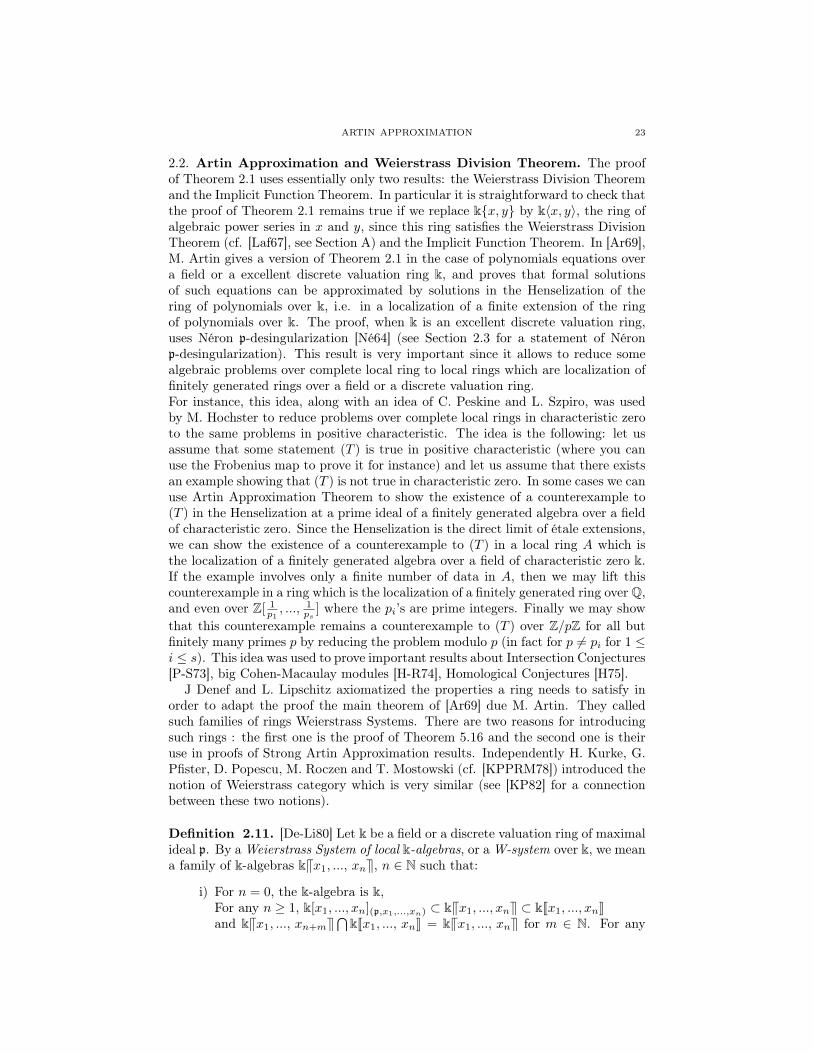
Remark 2.10. Let I be the ideal generated by f1,..., fr. The formal solu-tion y(x) of f = 0 induces a k{x}-morphism k{x, y} −→ kJxK defined by thesubstitution of y(x) for y. Then I is included in the kernel of this morphismthus, by the universal property of the quotient ring, this morphism induces ak{x}-morphism ψ : k{x,y}
I −→ kJxK. On the other hand, any k{x}-morphismψ : k{x,y}
I −→ kJxK is clearly defined by substituting for y a formal power seriesy(x) such that f(x, y(x)) = 0.
Thus we can reformulate Theorem 2.7 as follows: Let ψ : k{x,y}I −→ kJxK be
the k{x}-morphism defined by the formal power series solution y(x). Then thereexist an analytic k{x}-algebra D := k{x, z} and k{x}-morphisms C −→ D (definedvia the convergent power series solution y(x, z) of f = 0) and D −→ kJxK (definedby substituting z(x) for z) such that the following diagram commutes:
k{x}ϕ //
��
kJxK
k{x,y}I
ψ
88
// D := k{x, z}
OO
We will use and generalize this formulation later (see Theorem 2.16)
ARTIN APPROXIMATION 23
2.2. Artin Approximation and Weierstrass Division Theorem. The proofof Theorem 2.1 uses essentially only two results: the Weierstrass Division Theoremand the Implicit Function Theorem. In particular it is straightforward to check thatthe proof of Theorem 2.1 remains true if we replace k{x, y} by k〈x, y〉, the ring ofalgebraic power series in x and y, since this ring satisfies the Weierstrass DivisionTheorem (cf. [Laf67], see Section A) and the Implicit Function Theorem. In [Ar69],M. Artin gives a version of Theorem 2.1 in the case of polynomials equations overa field or a excellent discrete valuation ring k, and proves that formal solutionsof such equations can be approximated by solutions in the Henselization of thering of polynomials over k, i.e. in a localization of a finite extension of the ringof polynomials over k. The proof, when k is an excellent discrete valuation ring,uses Néron p-desingularization [Né64] (see Section 2.3 for a statement of Néronp-desingularization). This result is very important since it allows to reduce somealgebraic problems over complete local ring to local rings which are localization offinitely generated rings over a field or a discrete valuation ring.For instance, this idea, along with an idea of C. Peskine and L. Szpiro, was usedby M. Hochster to reduce problems over complete local rings in characteristic zeroto the same problems in positive characteristic. The idea is the following: let usassume that some statement (T ) is true in positive characteristic (where you canuse the Frobenius map to prove it for instance) and let us assume that there existsan example showing that (T ) is not true in characteristic zero. In some cases we canuse Artin Approximation Theorem to show the existence of a counterexample to(T ) in the Henselization at a prime ideal of a finitely generated algebra over a fieldof characteristic zero. Since the Henselization is the direct limit of étale extensions,we can show the existence of a counterexample to (T ) in a local ring A which isthe localization of a finitely generated algebra over a field of characteristic zero k.If the example involves only a finite number of data in A, then we may lift thiscounterexample in a ring which is the localization of a finitely generated ring over Q,and even over Z[ 1
p1, ..., 1
ps] where the pi’s are prime integers. Finally we may show
that this counterexample remains a counterexample to (T ) over Z/pZ for all butfinitely many primes p by reducing the problem modulo p (in fact for p 6= pi for 1 ≤i ≤ s). This idea was used to prove important results about Intersection Conjectures[P-S73], big Cohen-Macaulay modules [H-R74], Homological Conjectures [H75].
J Denef and L. Lipschitz axiomatized the properties a ring needs to satisfy inorder to adapt the proof the main theorem of [Ar69] due M. Artin. They calledsuch families of rings Weierstrass Systems. There are two reasons for introducingsuch rings : the first one is the proof of Theorem 5.16 and the second one is theiruse in proofs of Strong Artin Approximation results. Independently H. Kurke, G.Pfister, D. Popescu, M. Roczen and T. Mostowski (cf. [KPPRM78]) introduced thenotion of Weierstrass category which is very similar (see [KP82] for a connectionbetween these two notions).
Definition 2.11. [De-Li80] Let k be a field or a discrete valuation ring of maximalideal p. By a Weierstrass System of local k-algebras, or a W-system over k, we meana family of k-algebras kVx1, ..., xnW, n ∈ N such that:
i) For n = 0, the k-algebra is k,For any n ≥ 1, k[x1, ..., xn](p,x1,...,xn) ⊂ kVx1, ..., xnW ⊂ kJx1, ..., xnKand kVx1, ..., xn+mW
⋂kJx1, ..., xnK = kVx1, ..., xnW for m ∈ N. For any
24 HERWIG HAUSER, GUILLAUME ROND
permutation σ of {1, ..., n} if f ∈ kVx1, ..., xnW, then f(xσ(1), ..., xσ(n)) ∈kVx1, ..., xnW.
ii) Any element of kVxW, x = (x1, ..., xn), which is a unit in kJxK, is a unit inkVxW.
iii) If f ∈ kVxW and p divides f in kJxK then p divides f in kVxW.iv) Let f ∈ (p, x)kVxW such that f 6= 0. Suppose that f ∈ (p, x1, ..., xn−1, x
sn)
but f /∈ (p, x1, ..., xn−1, xs−1n ). Then for any g ∈ kVxW there exist a unique
q ∈ kVxW and a unique r ∈ kVx1, ..., xn−1W[xn] with deg xnr < d such that
g = qf + r.v) (if char(k) > 0) If y ∈ (p, x1, ..., xx)kJx1, ..., xnKm and f ∈ kVy1, ..., ymW
such that f 6= 0 and f(y) = 0, then there exists g ∈ kVyW irreduciblein kVyW such that g(y) = 0 and such that there does not exist any unitu(y) ∈ kVyW with u(y)g(y) =
∑α∈Nn aαy
pα (aα ∈ k).vi) (if char(k/p) 6= 0) Let (k/p)VxW be the image of kVxW under the projection
kJxK −→ (k/p)JxK. Then (k/p)VxW satisfies v).
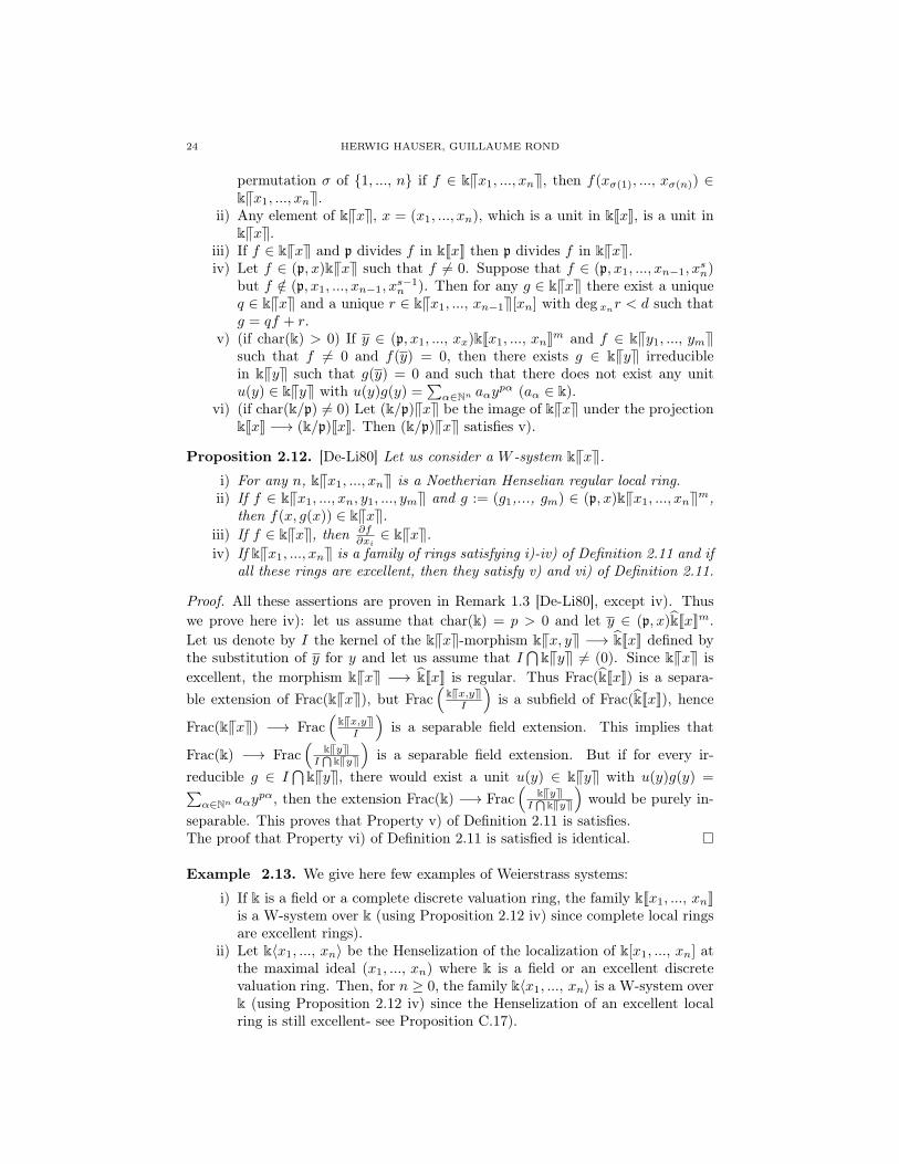
Proposition 2.12. [De-Li80] Let us consider a W -system kVxW.
i) For any n, kVx1, ..., xnW is a Noetherian Henselian regular local ring.ii) If f ∈ kVx1, ..., xn, y1, ..., ymW and g := (g1,..., gm) ∈ (p, x)kVx1, ..., xnWm,
then f(x, g(x)) ∈ kVxW.iii) If f ∈ kVxW, then ∂f
∂xi∈ kVxW.
iv) If kVx1, ..., xnW is a family of rings satisfying i)-iv) of Definition 2.11 and ifall these rings are excellent, then they satisfy v) and vi) of Definition 2.11.
Proof. All these assertions are proven in Remark 1.3 [De-Li80], except iv). Thuswe prove here iv): let us assume that char(k) = p > 0 and let y ∈ (p, x)kJxKm.Let us denote by I the kernel of the kVxW-morphism kVx, yW −→ kJxK defined bythe substitution of y for y and let us assume that I
⋂kVyW 6= (0). Since kVxW is
excellent, the morphism kVxW −→ kJxK is regular. Thus Frac(kJxK) is a separa-ble extension of Frac(kVxW), but Frac
(kVx,yWI
)is a subfield of Frac(kJxK), hence
Frac(kVxW) −→ Frac(
kVx,yWI
)is a separable field extension. This implies that
Frac(k) −→ Frac(
kVyWI⋂
kVyW
)is a separable field extension. But if for every ir-
reducible g ∈ I⋂kVyW, there would exist a unit u(y) ∈ kVyW with u(y)g(y) =∑
α∈Nn aαypα, then the extension Frac(k) −→ Frac
(kVyW
I⋂
kVyW
)would be purely in-
separable. This proves that Property v) of Definition 2.11 is satisfies.The proof that Property vi) of Definition 2.11 is satisfied is identical. �
Example 2.13. We give here few examples of Weierstrass systems:
i) If k is a field or a complete discrete valuation ring, the family kJx1, ..., xnKis a W-system over k (using Proposition 2.12 iv) since complete local ringsare excellent rings).
ii) Let k〈x1, ..., xn〉 be the Henselization of the localization of k[x1, ..., xn] atthe maximal ideal (x1, ..., xn) where k is a field or an excellent discretevaluation ring. Then, for n ≥ 0, the family k〈x1, ..., xn〉 is a W-system overk (using Proposition 2.12 iv) since the Henselization of an excellent localring is still excellent- see Proposition C.17).
ARTIN APPROXIMATION 25
iii) The family k{x1, ..., xn} (the ring of convergent power series in n variablesover a valued field k) is a W-system over k.
iv) The family of Gevrey power series in n variables over a valued field k is aW-system [Br86].
Then we have the following Approximation result (the case of k〈x〉 where k is afield or a discrete valuation ring is proven in [Ar69], the general case is proven in[De-Li80]):
Theorem 2.14. [Ar69][De-Li80] Let kVxW be a W-system over k, where k is a fieldor a discrete valuation ring with prime p. Let f ∈ kVx, yWr and y ∈ (p, x)kJxKmsatisfy
f(x, y) = 0.
Then, for any c ∈ N, there exists a convergent power series solution y ∈ (p, x)kVxWm,
f(x, y) = 0 such that y − y ∈ (p, x)c.
Let us mention that Theorem 2.7 extends also for Weierstrass systems (see[Ron10b]).
2.3. Néron’s desingularization and Popescu’s Theorem. During the 70’s andthe 80’s one of the main goals about Artin Approximation Problem was to find nec-essary and sufficient conditions on a local ring A for it having the Artin Approxi-mation Property, i.e. such that the set of solutions in Am of any system of algebraicequations (S) in m variables with coefficients in A is dense for the Krull topologyin the set of solutions of (S) in Am. Let us recall that the Krull topology on Ais the topology induced by the following norm: |a| := e−ord(a) for all a ∈ A\{0}.The problem was to find a way of proving approximation results without usingWeierstrass Division Theorem.
Remark 2.15. Let P (y) ∈ A[y] satisfy P (0) ∈ mA and ∂P∂y (0) /∈ mA. Then, by the
Implicit Function Theorem for complete local rings, P (y) has a unique root in Aequal to 0 modulo mA. Thus if we want being able to approximate roots of P (y) inA by roots of P (y) in A, a necessary condition is that the root of P (y) constructedby the Implicit Function Theorem is in A. Thus it is clear that if a local ring Ahas the Artin Approximation Property then A is necessarily Henselian.
In fact M. Artin conjectured that a sufficient condition would be that A is anexcellent Henselian local ring (Conjecture (1.3) [Ar70]). The idea to prove thisconjecture is to generalize Płoski’s Theorem 2.7 and a theorem of desingularizationof A. Néron [Né64]. This generalization is the following (for the definitions seeAppendix B):
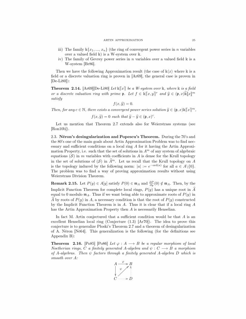
Theorem 2.16. [Po85] [Po86] Let ϕ : A −→ B be a regular morphism of localNoetherian rings, C a finitely generated A-algebra and ψ : C −→ B a morphismof A-algebras. Then ψ factors through a finitely generated A-algebra D which issmooth over A:
Aϕ //
��
B
C
ψ>>
// D
OO
26 HERWIG HAUSER, GUILLAUME ROND
Historically this theorem has been proven by A. Néron [Né64] when A and B arediscrete valuation rings. Then several authors gave proofs of particular cases (seefor instance [Po80], [Br83b] [Ar-De83], [Ar-Ro88], or [Rot87] - in this last paperthe result is proven in the equicharacteristic zero case) until D. Popescu [Po85][Po86] proved the general case. Then, several authors gave simplified proofs orstrengthened the result [Og94], [Sp99], [Sw98]. This result is certainly the mostdifficult to prove among all the results presented in this paper. We will just give aslight hint of the proof of this result here since there exist very nice presentations ofthe proof elsewhere (see [Sw98] in general, [Qu97] or [Po00] in the equicharacteristiczero case).Since A −→ A is regular if A is excellent, I is an ideal of A and A := lim
←−AIn , we get
the following result (exactly as Theorem 2.7 implies Theorem 2.1):
Theorem 2.17. Let (A, I) be an excellent Henselian pair. Let f(y) ∈ A[y]r andy ∈ Am satisfy f(y) = 0. Then, for any c ∈ N, there exists y ∈ Am such thaty − y ∈ IcA, and f(y) = 0.
Proof. The proof goes as follows: let us denote C := A[y]J where J is the ideal
generated by f1,..., fr. The formal solution y ∈ A defines a A-morphism ϕ :
C −→ A (see Remark 2.10). By Theorem 2.16, since A −→ A is regular (ExampleB.4), there exists a smooth A-algebra D factorizing this morphism. After sometechnical reductions we may assume that the morphism A −→ D decomposes asA −→ A[z] −→ D where z = (z1, ..., zs) and A[z] −→ D is standard étale. Letus choose z ∈ As such that z − z ∈ mcAA
s (z is the image of z in As). Thisdefines a morphism A[z] −→ A. Then A −→ D
(z1−z1,...,zs−zs) is standard étale andadmits a section in A
mcA. Since A is Henselian, this section lifts to a section in A
by Proposition C.9. This section composed with A[z] −→ A defines a A-morphismD −→ A, and this latter morphism composed with C −→ D yields a morphismϕ : C −→ A such that ϕ(zi)− ϕ(zi) ∈ mcAA for 1 ≤ i ≤ m. �
Remark 2.18. Let (A, I) be a Henselian pair and let J be an ideal of A. Byapplying this result to the Henselian pair
(BJ ,
IBJ
)we can prove the following (using
the notation of Theorem 2.17): if f(y) ∈ JA then there exists y ∈ Am such thatf(y) ∈ J and y − y ∈ IcA.
Remark 2.19. In [Rot90], C. Rotthaus proves the converse of Theorem 2.17 inthe local case: if A is a Noetherian local ring that satisfies Theorem 2.17, then Ais excellent. In particular Weierstrass systems are excellent local rings. Previouslythis problem had been studied in [C-P81] and [Br83a].
Remark 2.20. Let A be a Noetherian ring and I be an ideal of A. If we assumethat f1(y),..., fr(y) ∈ A[y] are linear, then Theorem 2.17 may be proven easily inthis case since A −→ A is flat (see Example 2). The proof of this flatness resultuses the Artin-Rees Lemma.
Example 2.21. If A is an excellent integral local domain let us denote by Ah itsHenselization. Then Ah is the ring of algebraic elements of A over A. In particular,if k is a field then k〈x〉 is the ring of formal power series which are algebraic overk[x].Indeed A −→ Ah is a filtered limit of algebraic extension, thus Ah is a subring of
ARTIN APPROXIMATION 27
the ring of algebraic elements of A over A.On the other hand if f ∈ A is algebraic over A, then f satisfies an equation
a0fd + a1f
d−1 + · · ·+ ad = 0
where ai ∈ A for all i. Thus for c large enough there exists f ∈ Ah such thatf satisfies the same polynomial equation and f − f ∈ mcA (by Theorem 2.17 andTheorem C.17). Since
⋂cm
cA = (0) and a polynomial equation has a finite number
of roots, this proves that f = f for c large enough and f ∈ Ah.Example 2.22. The strength of this result comes from the fact that it worksfor rings that does not satisfy the Weierstrass Preparation Theorem. For exampleTheorem 2.17 applies to the local ring B = A〈x1, ..., xn〉 where A is an excellentHenselian local ring (the main example being A = kJtK〈x〉 where t and x are multi-variables). Indeed, this ring is the Henselization of A[x1, ..., xn]mA+(x1,...,xn). ThusB is an excellent local ring by Example B.4 and Proposition C.17.This case was the main motivation of D. Popescu for proving Theorem 2.16 (see also[Ar70]), since this case implies a nested Artin Approximation result (see Theorem5.8).Previous particular cases of this application had been studied before: see [Pf-Po81]for a direct proof that V Jx1K〈x2〉 satisfies Theorem 2.17, when V is a completediscrete valuation ring, and [BDL83] for the ring kJx1, x2K〈x3, x4, x5〉.Hint of the proof of Theorem 2.16. Let A be a Noetherian ring and C be a A-algebra of finite type, C = A[y1,...ym]
I with I = (f1, ...., fr). We denote by ∆g the
ideal ofA[y] generated by the h×hminors of the Jacobian matrix(∂gi∂yj
)1≤i≤h,1≤j≤m
for g := (g1, ..., gh) ⊂ I. We define the ideal
HC/A :=
√∑g
∆g((g) : I)C
where the sum runs over all g := (g1, ..., gh) ⊂ I and h ∈ N. This ideal is indepen-dent of the presentation of C and it defines the singular locus of C over A:
Lemma 2.23. For any p ∈ Spec(C), Cp is smooth over A if and only if HC/A 6⊂ p.
We have the following property:
Lemma 2.24. Let C and C ′ be two A-algebras of finite type and let A −→ C −→ C ′
be two morphisms of A-algebras. Then HC′/C
⋂√HC/AC ′ = HC′/C
⋂HC′/A.
The idea of the proof of Theorem 2.16 is the following: if HC/AB 6= B, thenwe replace C by a A-algebra of finite type C ′ such that HC/AB is a proper sub-ideal of HC′/AB. Using the Noetherian assumption, after a finite number we haveHC/AB = B. Then we use the following proposition:
Proposition 2.25. Using the notation of Theorem 2.16, let us assume that HC/AB =B. Then ψ factors as in Theorem 2.16.
Proof of Proposition 2.25. Let (c1, ..., cs) be a system of generators of HC/A. Then
1 =
s∑i=1
biψ(ci) for some bi’s in B. Let us define
D :=C[z1, ..., zs]
(1−∑si=1 cizi)
.
28 HERWIG HAUSER, GUILLAUME ROND
We construct a morphism of C-algebra D −→ B by sending zi onto bi, 1 ≤ i ≤ s.It is easy to check Dci is a smooth C-algebras, thus ci ∈ HD/C by Lemma 2.23,and HC/AD ⊂ HD/C . By Lemma 2.24, since 1 ∈ HC/AD, we see that 1 ∈ HD/A.By Lemma 2.23, this proves that D is a smooth A-algebra.
�
Now to increase the size of HC/AB we use the following proposition:
Proposition 2.26. Using the notation of Theorem 2.16, let p be a minimal primeideal of HC/AB. Then there exist a factorization of ψ : C −→ D −→ B such thatD is finitely generated over A and
√HC/AB (
√HD/AB 6⊂ p.
The proof of Proposition 2.26 is done by induction on height(p). Thus there istwo cases to prove: first the case ht(p) = 0 which is equivalent to prove Theorem2.16 for Artinian rings, then the reduction ht(p) = k + 1 to the case ht(p) = k.This last case is quite technical, even in the equicharacteristic zero case (i.e. whenA contains Q, see [Qu97] for a good presentation of this case). In the case Adoes not contain Q there appear more problems due to the existence of inseparableextensions of residue fields. In this case the André homology is the good tool tohandle these problems (see [Sw98]).
�
3. Strong Artin Approximation
We review here results about the Strong Approximation Property. There isclearly two different cases: the first case is when the base ring is a discrete valuationring (where life is easy!) and the second case is the general case (where life is lesseasy).
3.1. Greenberg’s Theorem: the case of a discrete valuation ring. Let Vbe a Henselian discrete valuation ring, mV its maximal ideal and K be its fieldof fractions. Let us denote by V the mV -adic completion of V and by K its fieldof fractions. If char(K) > 0, let us assume that K −→ K is a separable fieldextension (in this case this is equivalent to V being excellent, see Example B.2 iii)and Example B.4 iv)).
Theorem 3.1 (Greenberg’s Theorem). [Gre66] If f(y) ∈ V [y]r, then there exista, b ≥ 0 such that
∀c ∈ N ∀y ∈ V m such that f(y) ∈ mac+bV
∃y ∈ V m such that f(y) = 0 and y − y ∈ mcV .
Sketch of proof. We will give the proof in the case char(K) = 0. The result is provenby induction on the height of the ideal generated by f1(y),..., fr(y). Let us denoteby I this ideal. We will denote by ν, the mV -adic order on V which is a valuationby assumption.There exists an integer e ≥ 1 such that
√Ie ⊂ I. Then f(y) ∈ mecV for all f ∈ I
implies that f(y) ∈ mcV for all f ∈√I since V is a valuation ring. Moreover if√
I = P1
⋂· · ·⋂Ps is prime decomposition of
√I, then f(y) ∈ mscV for all f ∈
√I
implies that f(y) ∈ mcV for all f ∈ Pi for some i. This allows us to assume that Iis a prime ideal of V [y].Let h be the height of I. If h = m+ 1, then I is a maximal ideal of V [y] and thus
ARTIN APPROXIMATION 29
it contains some non zero element of V denoted by v. Then there does not existy ∈ V m such that f(y) ∈ m
ν(v)+1V for all f ∈ I. Thus the theorem is true for a = 0
and b = ν(v) + 1.Let us assume that the theorem is proven for ideals of height h+ 1 and let I be aprime ideal of height h. As in the proof of Theorem 2.1, we may assume that r = hand that the determinant of the Jacobian matrix of f , denoted by δ, is not in I.Let us denote J := I + (δ). Since ht(J) = h+ 1, by the inductive hypothesis, thereexist a, b ≥ 0 such that
∀c ∈ N ∀y ∈ V m such that f(y) ∈ mac+bV ∀f ∈ J∃y ∈ V m such that f(y) = 0 ∀f ∈ J and yj − yj ∈ mcV , 1 ≤ j ≤ m.
Then let c ∈ N and y ∈ V m satisfy f(y) ∈ m(2a+1)c+2bV for all f ∈ I. If δ(y) ∈ mac+bV ,
then f(y) ∈ mac+bV for all f ∈ J and the result is proven by the inductive hypothesis.If δ(y) /∈ mac+bV , then fi(y) ∈ (δ(y))2mcV for 1 ≤ i ≤ r. Then the result comes fromthe following result.
�
Theorem 3.2 (Tougeron’s Implicit Function Theorem). Let A be a Henselianlocal ring and f(y) ∈ A[y]r, y = (y1, ..., ym), m ≥ r. Let δ(x, y) be a r× r minor ofthe Jacobian matrix ∂(f1,...,fr)
∂(y1,...,ym) . Let us assume that there exists y ∈ Am such that
fi(y) ∈ (δ(y))2mcA for all 1 ≤ i ≤ rand for some c ∈ N. Then there exists y ∈ Am such that
fi(y) = 0 for all 1 ≤ i ≤ r, and y − y ∈ (δ(y))mcA.
Proof. The proof is completely similar to the proof of Theorem 2.4. �
In fact we can prove the following result whose proof is identical to the proof ofTheorem 3.1:
Theorem 3.3. [Sc83] Let V be a complete discrete valuation ring and f(y, z) ∈V JyK[z]r, where z := (z1, ..., zs). Then there exist a, b ≥ 0 such that
∀c ∈ N ∀y ∈ (mV V )m, ∀z ∈ V s such that f(y, z) ∈ mac+bV
∃y ∈ (mV V )m, ∃z ∈ V s such that f(y, z) = 0 and y − y, z − z ∈ mcV .
Remark 3.4. M. Greenberg proved this result in order to study Ci fields. Previousresults about Ci fields had been already been studied, in particular by S. Lang in[Lan52] where appeared for the first time a particular case of Artin ApproximationTheorem (see Theorem 11 and its corollary in [Lan52]).
Remark 3.5. In the case f(y) has no solution in V , we can choose a = 0 andTheorem 3.1 asserts there exists a constant b such that f(y) has no solution in V
mbV
.
Remark 3.6. The valuation ν of V defines a ultrametric norm on K: we define itas ∣∣∣y
z
∣∣∣ := eν(z)−ν(y), ∀y, z ∈ V \{0}.
This norm defines a distance on V m, for any m ∈ N∗, denoted by d(., .) and definedby
d(y, z) :=m
maxk=1|yk − zk| .
30 HERWIG HAUSER, GUILLAUME ROND
Then Theorem 3.1 can be reformulated as a Łojasiewicz Inequality:
∃a ≥ 1, C > 0 s.t. |f(y)| ≥ Cd(f−1(0), y)a ∀y ∈ V m.
This Łojasiewicz Inequality is well known for algebraic or analytic functions andTheorem 3.1 can be seen as a generalization of this Łojasiewicz Inequality for al-gebraic or analytic functions defined over V . If V = kJtK where k is a field, thereis very few results known about the geometry of algebraic varieties defined overV . It is a general problem to extend classical results of differential or analytic ge-ometry over R or C to this setting. See for instance [H-M94], [B-H10] (extensionof Rank Theorem), [FB-PP2] (Extension of Curve Selection Lemma), [Hic05] forsome results in this direction.
For any c ∈ N let us denote by β(c) the smallest integer such that:for all y ∈ V m such that f(y) ∈ (x)β(c), there exists y ∈ V m such that f(y) = 0 andy− y ∈ (x)c. Greenberg’s Theorem asserts that such a function β : N −→ N existsand that it is bounded by an affine function. We call this function β the Greenbergfunction of f . We can remark that the Greenberg function is an invariant of theintegral closure of the ideal generated by f1,..., fr:
Lemma 3.7. Let us consider f(y) ∈ V [y]r and g(y) ∈ V [y]q. Let us denote by βfand βg their Greenberg functions. Let I (resp. J) be the ideal of V [y] generated byf1(y),..., fr(y) (resp. g1(y),..., gq(y)). If I = J then βf = βg. The same is truefor Theorem 3.3.
Proof. Let I be an ideal of V and y ∈ V m. We remark that
f1(y), ..., fr(y) ∈ I ⇐⇒ g(y) ∈ I ∀g ∈ I.
Then by replacing I by (0) and mcV , for all c ∈ N, we see that βf depends only onI.Now, for any c ∈ N, we have:
g(y) ∈ mcV ∀g ∈ I ⇐⇒ ν(g(y)) ≥ c ∀g ∈ I
⇐⇒ ν(g(y)) ≥ c ∀g ∈ I⇐⇒ g(y) ∈ mcV ∀g ∈ I.
Thus βf depends only on I. �
In general, it is a difficult problem to compute the Greenberg function of anideal I. It is even a difficult problem to bound this function in general. If weanalyze carefully the proof of Greenberg’s Theorem, using classical effective resultsin commutative algebra, we can prove the following result:
Theorem 3.8. [Ron10a] Let k be a characteristic zero field and V := kJtK wheret is a single variable. Then there exists a function
N2 −→ N
(m, d) 7−→ a(m, d)
which is a polynomial function in d whose degree is exponential in m, such that forany vector f(y) ∈ k[t, y]r of polynomials of total degree ≤ d, the Greenberg functionof f is bounded by c 7−→ a(m, d)(c+ 1). Here m denotes the size of y.
ARTIN APPROXIMATION 31
Moreover let us remark that, in the proof of Theorem 3.1, we proved a particularcase of the following inequality:
βI(c) ≤ 2βJ(c) + c, ∀c ∈ Nwhere J is the Jacobian Ideal of I (for a precise definition of the Jacobian Idealin general and a general proof of this inequality let see [El73]). The coefficient 2comes from the use of Tougeron’s Implicit Function Theorem. We can sharpen thisbound in the following particular case:
Theorem 3.9. [Hic93] Let k be an algebraically closed field of characteristic zeroand V := kJtK where t is a single variable. Let f(y) ∈ V JyK be one power series. Letus denote by J the ideal of V JyK generated by f(y), ∂f∂t (y), ∂f
∂y1(y),..., ∂f
∂ym(y), and
let us denote by βf the Greenberg function of (f) and by βJ the Greenberg functionof J . Then
βf (c) ≤ βJ(c) + c ∀c ∈ N.This bound may be used to find sharp bounds of some Greenberg functions (see
Remark 3.11).On the other hand we can describe the behaviour of β in the following case:
Theorem 3.10. [De84][De-Lo99] Let V be Zp or a Henselian discrete valuationring whose residue field is an algebraically closed field of characteristic zero. Letus denote by mV the maximal ideal of V . Let us denote by β the Artin functionof f(y) ∈ V [y]r. Then there exists a finite partition of N in congruence classessuch that on each such congruence class the function c 7−→ β(c) is linear for c largeenough.
Hints on the proof in the case the residue field has characteristic zero. Let us con-sider the following first order language of three sorts:
1) the field (K := Frac(V ),+,×, 0, 1)2) the group (Z,+, <,≡d (∀d ∈ N∗), 0) (≡d is the relation a ≡d b if and only
if a− b is divisible by d for a, b ∈ Z)3) the residue field (k := Frac
(VmV
),+,×, 0, 1)
with both following functions:a) ν : K −→ Z∗b) ac : K −→ k ("angular component")
The function ν is the valuation of the valuation ring V . The function ac may becharacterized by axioms, but here let us just give an example: let us assume thatV = kJtK. Then ac is defined by ac(0) = 0 and ac
(∑∞n=n0
antn)
= an0if an0
6= 0.The second sort (Z,+, <,≡d, 0) admits elimination of quantifiers ([Pr29]) and theelimination of quantifiers of (k,+,×, 0, 1) is a classical result of Chevalley. J. Pasproved that the first sort language and the three sorted language admits eliminationof quantifiers [Pa89]. This means that any subset of Kn1 × Zn2 × kn3 defined by afirst order formula in this three sorts language (i.e. a logical formula involving 0,1,+ ,× (but not a× b where a and b are integers), (, ), =, <, ∧, ∨, ¬, ∀, ∃, ν, ac,and variables for elements of K, Z and k may be defined by a formula involving thesame symbols except ∀, ∃.Then we see that β is defined by the following logical sentence:
[∀c ∈ N ∀y ∈ Km (ν(f(y)) ≥ β(c)) ∧ (ν(y) ≥ 0) ∃y ∈ Km (f(y) = 0 ∧ ν(y − y) ≥ c)]
32 HERWIG HAUSER, GUILLAUME ROND
∧ [∀c ∈ N ∃y ∈ Km (ν(f(y)) ≥ β(c) + 1) ∧ (ν(y) ≥ 0)
¬∃y ∈ Km (f(y) = 0 ∧ ν(y − y) ≥ c)]Applying the latter elimination of quantifiers result we see that β(c) may be definedwithout ∀ and ∃. Thus β(c) is defined by a formula using +, <, ≡d (for a finite setof integers d). This proves the result.The case where V = Zp needs more work since the residue field of Zp is notalgebraically closed, but the idea is the same. �
Remark 3.11. When V = C{t}, t being a single variable, it is tempting to linktogether the Greenberg function of a system of equations with coefficients in Vand some geometric invariants of the germ of complex set defined by this system ofequations. This has been done in several cases:
i) In [El89], a bound (involving the multiplicity and the Milnor number) of theGreenberg function is given when the system of equations defines a curvein Cm.
ii) Using Theorem 3.9 [Hic93] gives the following bound of the Greenbergfunction β of a germ of complex hypersurface with an isolated singularity:β(c) ≤ bλcc+c for all c ∈ N, and this bound is sharp for plane curves. Hereλ denotes the Łojasiewicz exponent of the germ, i.e.
λ := inf {θ ∈ R / ∃C > 0 ∃U neighborhood of 0 in Cm,
|f(z)|+∣∣∣∣ ∂f∂z1 (z)
∣∣∣∣+ · · ·+∣∣∣∣ ∂f∂zm (z)
∣∣∣∣ ≥ C|z|θ ∀z ∈ U} .iii) [Hic04] makes the complete computation of the Greenberg function of a
branch of plane curve and proves that it is a topological invariant. Thiscomputation has been done for several branches in [Sa10]. Some particularcases depending on the Newton polygon of the plane curve singularity arecomputed in [Wa78].
Finally we mention the following recent result that extends Theorem 3.1 to non-Noetherian valuation rings and whose proof is based on ultraproducts methods usedin [BDLvdD79] to prove Theorem 3.1 (see 3.3):
Theorem 3.12. [M-B11] Let V be a Henselian valuation ring and ν : V −→ Γ
its associated valuation. Let us denote by V its mV -adic completion, K := Frac(V )
and K := Frac(V ). Let us assume that K −→ K is a separable extension. Then forany f(y) ∈ V [y]r there exist a ∈ N, b ∈ Γ+ such that
∀c ∈ Γ ∀y ∈ V m (ν(f(y)) ≥ ac+ b) =⇒ ∃y ∈ V m (f(y) = 0 ∧ ν(y − y) ≥ c) .
3.2. Strong Artin Approximation Theorem: the general case. In the gen-eral case (when V is not a valuation ring), there still exists an approximationfunction β. We have the following results:
Theorem 3.13. [Ar68][BDLvdD79] Let k be a field. For all n,m, d ∈ N, thereexists a function βn,m,d : N −→ N such that the following holds:Set x := (x1, ..., xn) and y := (y1, ..., ym). Then for all f(x, y) ∈ k[x, y]r of totaldegree ≤ d, for all c ∈ N, for all y(x) ∈ kJxKm such that
f(x, y(x)) ∈ (x)βn,m,d(c),
ARTIN APPROXIMATION 33
there exists y(x) ∈ kJxKm such that f(y(x)) = 0 and y(x)− y(x) ∈ (x)c.
Remark 3.14. By following the proof of M. Artin, D. Lascar proved that thereexists a recursive function β that satisfies the conclusion of Theorem 3.13 [Las78].But the proof of Theorem 3.13 uses a double induction on the height of the ideal(like in Theorem 3.1) and on n (like in Theorem 2.1). In particular, in order toapply the Jacobian Criterion, we need to work with prime ideals, and replace theoriginal ideal I generated by f1,..., fr by one of its associated prime and then makea reduction to n − 1 variables. But the bounds of the degree of the generators ofsuch associated prime may be very large compared to the degree of the generatorsof I. This is essentially the reason why the proof of this theorem does not givemuch more information about the growth of β than Lascar’s result.
Theorem 3.15. [Pf-Po75] [Po86] Let A be a complete local ring whose maximalideal is denoted by mA. Let f(y, z) ∈ AJyK[z]r, with z := (z1, ..., zs). Then thereexists a function β : N −→ N such that the following holds:For any c ∈ N and any y ∈ (mA.A)m and z ∈ As such that f(y, z) ∈ m
β(c)A , there
exists y ∈ (mA.A)m and z ∈ As such that f(y, z) = 0 and y − y, z − z ∈ mcA.
Example 3.16. [Sp94] Set f(x1, x2, y1, y2) := x1y21 − (x1 + x2)y22 . Set
√1 + t = 1 +
∑n≥1
antn ∈ CJtK
be the power series such that√
1 + t2
= 1 + t. For any c ∈ N set y(c)2 (x) := xc1 andy(c)1 (x) := xc1 +
∑cn=1 anx
c−n1 xn2 . Then
f(x1, x2, y(c)1 (x), y
(c)2 (x)) ∈ (x2)c.
On the other side the equation f(x1, x2, y1(x), y2(x)) = 0 has no other solution(y1(x), y2(x)) ∈ kJxK2 but (0, 0). This proves that Theorem 3.17 is not valid forgeneral Henselian pairs since (kJx1, x2K, (x2)) is a Henselian pair.Let us notice that L. Moret-Bailley proved that if a pair (A, I) satisfies Theorem3.17, then A has to be an excellent Henselian local ring [M-B07]. It is still open toknow under which conditions on I the pair (A, I) satisfies Theorem 3.17 when A isan excellent Henselian local ring.
Corollary 3.17. [Pf-Po75] [Po86] Let A be an excellent Henselian local ring whosemaximal ideal is denoted by mA and let f(y) ∈ A[y]r. Then there exists a functionβ : N −→ N such that:
∀c ∈ N, ∀y ∈ Am such that f(y) ∈ mβ(c)A
∃y ∈ Am such that f(y) = 0 and y − y ∈ mcA.
Corollary 3.18. [Wa75][De-Li80] Let kVxW be a W-system over k, where k is afield or a discrete valuation ring with prime p. Let f(x, y) ∈ kVx, yWr. Then thereexists a function β : N −→ N such that for any c ∈ N and any y ∈ (p, x)kJxKm
such that f(x, y) ∈ (p, x)β(c), there exists y ∈ (p, x)kVxWm such that f(x, y) = 0and y − y ∈ (p, x)c.
Proof. We first apply Theorem 3.15 then we apply Theorem 2.14. �
34 HERWIG HAUSER, GUILLAUME ROND
Remark 3.19. As for Theorem 3.1, Corollary 3.17 implies that, if f(y) has nosolution in A, there exists a constant c such that f(y) has no solution in A
mcA.
Definition 3.20. Let f be as in Theorem 3.15 or Corollary 3.17. The leastfunction β that satisfies these theorems is called the Artin function of f .
Remark 3.21. As before, the Artin function of f depends only on the integralclosure of the ideal I generated by f1,..., fr (see Lemma 3.7).
Remark 3.22. Let f(y) ∈ AJyKr and y ∈ (mA)m satisfy f(y) ∈ mcA and let usassume that A −→ B := AJyK
(f(y)) is a smooth morphism. This morphism is local thusit splits as A −→ C := A[z]mA+(z) −→ B such that C −→ B is étale (see DefinitionC.5) and z := (z1, ..., zs). We remark that y defines a morphism of A-algebrasϕ : B −→ A
mcA. Let us choose any z ∈ As such that zi − zi ∈ mcA for all 1 ≤ i ≤ s
(zi denotes the image of zi in Amc
A). Then A −→ B
(z1−z1,...,zs−z) is étale and admitsa section in A
mcA. By Proposition C.9, this section lifts to a section in A. Thus we
have a section B −→ A equal to ϕ modulo mcA.This proves that β(c) = c when A −→ AJyK
(f(y)) is smooth.
3.3. Ultraproducts and proofs of Strong Approximation type results. His-torically, M. Artin proved Theorem 3.13 in [Ar69] by slightly modifying the proofof Theorem 2.1, i.e. by an induction on n using the Weierstrass Division Theorem.Then some people tried to prove this kind of result in the same way, but this wasnot always easy, in particular when the base field was not a characteristic zero field(for example there is a gap in the inseparable case of [Pf-Po75]). Then four peo-ple introduced the use of ultraproducts to give easy proofs of this kind of StrongApproximation type results ([BDLvdD79] and [De-Li80]; see also [Po79] for thegeneral case). The general principle is the following: ultraproducts reduce StrongArtin Approximation Problems to Artin Approximation Problems. We will presenthere the main ideas.
Let us start with some terminology. A filter D (over N) is a non empty subsetof P(N), the set of subsets of N, that satisfies the following properties:
a) ∅ /∈ D, b) E , F ∈ D =⇒ E⋂F ∈ D, c) E ∈ D, E ⊂ F =⇒ F ∈ D.
A filter D is principal if D = {F / E ⊂ F} for some subset E of N. A ultrafilteris a filter which is maximal for the inclusion. It is easy to check that a filter D isa ultrafilter if and only if for any subset E of N, D contains E or its complementN − E . In the same way a ultrafilter is non-principal if and only if it contains thefilter E := {E ⊂ N / N − E is finite}. Zorn’s Lemma yields the existence of non-principal ultrafilters.
Let A be a Noetherian ring. Let D be a non-principal ultrafilter. We define theultrapower (or ultraproduct) of A as follows:
A∗ :={(ai)i∈N ∈
∏iA}
((ai) ∼ (bi) iff {i / ai = bi} ∈ D).
We have a morphism A −→ A∗ that sends a onto the class of (a)i∈N. We have thefollowing fundamental result:
ARTIN APPROXIMATION 35
Theorem 3.23. [C-K73] Let L be a first order language, let A be a structure for Land let D be an ultrafilter over N. Then for any (ai)i∈N ∈ A∗ and for any first orderformula ϕ(x), ϕ((ai)) is true in A∗ if and only if {i ∈ N / ϕ(ai) is true in A} ∈ D.
In particular we can deduce the following properties:The ultraprower A∗ is equipped with a structure of commutative ring. If A is a fieldthen A∗ is a field. If A is an algebraically closed field then A∗ is an algebraicallyclosed field. If A∗ is a local ring with maximal ideal mA then A∗ is a local ringwith maximal ideal m∗A defined by (ai)i ∈ m∗A if and only if {i / ai ∈ mA} ∈ D. IfA is a local Henselian ring, then A∗ is a local Henselian ring. In fact all these factsare elementary and can be checked directly by hand. Elementary proofs of theseresults can be found in [BDLvdD79].Nevertheless if A is Noetherian, then A∗ is not Noetherian in general, since Noethe-rianity is a condition on ideals of A and not on elements of A. For example, if A isa Noetherian local ring, then m∗∞ :=
⋂n≥0 m
∗An 6= (0) in general. But we have the
following lemma:
Lemma 3.24. [Po00] Let (A,mA) be a Noetherian complete local ring. Let usdenote A1 := A∗
m∗∞. Then A1 is a Noetherian complete local ring of same dimension
as A and the composition A −→ A∗ −→ A1 is flat.
In fact, since A is excellent and mAA1 is the maximal ideal of A1, it is not diffi-cult to prove that A −→ A1 is regular. Details can be found in [Po00].
Let us sketch the idea in the case of Theorem 3.17:
Sketch of the proof of Theorem 3.17. Let us assume that some system of algebraicequations over an excellent Henselian local ring A, denoted by f = 0, does notsatisfy Theorem 3.17. Using Theorem 2.17, we may assume that A is complete.Thus it means that there exist an integer c0 ∈ N and y(c) ∈ Am, ∀ c ∈ N, suchthat f(y(c)) ∈ mcA and there does not exists y(c) ∈ Am such that f(y(c)) = 0 andy(c) − y(c) ∈ mc0A .Let us denote by y the image of (y(c))c in (A∗)m. Since f(y) ∈ A[y]r, we mayassume that f(y) ∈ A∗[y]r using the morphism A −→ A∗. Then f(y) ∈ m∗∞.Thus f(y) = 0 in A1. Let us choose c > c0. Since A −→ A1 is regular and A isHenselian, following the proof of Theorem 2.17, for any c ∈ N there exists y ∈ Amsuch that f(y) = 0 and y − y ∈ mcAA1. Thus y − y ∈ mcAA
∗. Hence the set{i ∈ N / y − y(i) ∈ mcAA
∗} ∈ D is non-empty. This is a contradiction. �
We can also prove easily the following proposition with the help of ultraproducts:
Proposition 3.25. [BDLvdD79] Let f(x, y) ∈ C[x, y]r. For any 1 ≤ i ≤ m let Jibe a subset of {1, ..., n}.Let us assume that, for any c ∈ N, there exist y(c)i (x) ∈ C[xj , j ∈ Ji], 1 ≤ i ≤ m,such that
f(x, y(c)(x)) ∈ (x)c.
Then there exist yi(x) ∈ CJxj , j ∈ JiK, 1 ≤ i ≤ m, such that f(x, y(x)) = 0.
Proof. Let us denote by y ∈ C[x]∗ the image of (y(c))c. Then f(x, y) = 0 modulo(x)∗∞. It is not very difficult to check that C[x]∗
(x)∗∞' C∗JxK as C∗[x]-algebras. More-
over C∗ ' C as k-algebras (where k is the subfield of C generated by the coefficients
36 HERWIG HAUSER, GUILLAUME ROND
of f), since they are algebraically closed field of same transcendence degree over Qand same characteristic. Then the image of y by the isomorphism yields the desiredsolution in CJxK. �
Let us remark that the proof of this result remains valid if we replace C by anyalgebraically closed field k whose cardinal is strictly greater that the cardinal of N.If we replace C by Q, this result is no more true in general (see Example 5.23).
3.4. Effectivity of the behaviour of Artin functions: some examples. Ingeneral the proofs of Strong Artin Approximation results do not give much in-formation about the Artin functions, since ultraproducts methods use a proof bycontradiction (see also Remark 3.14). The problem of finding estimates of Artinfunctions was raised first in [Ar70] and very few general results are known (the onlyones in the case of Greenberg Theorem are Theorems 3.8, 3.9, 3.10 and Remark3.14 in the general case). We give here a list of examples for which we can give nontrivial effective behaviour about their Artin function.
3.4.1. Artin-Rees Lemma. The following result has been known for long by thespecialists and has been communicated to the author by M. Hickel:
Theorem 3.26. [Ron06a] Let f(y) ∈ A[y]r be a vector of linear polynomials withcoefficients in a Noetherian ring A. Let I be an ideal of A. Then there exists aconstant c0 ≥ 0 such that:
∀c ∈ ∀y ∈ Am such that f(y) ∈ Ic+c0
∃y ∈ Am such that f(y) = 0 and y − y ∈ Ic.
This theorem asserts that the function β of Theorem 3.17 is bounded by thefunction c −→ c+ c0. Moreover let us remark that this theorem is valid for generalNoetherian ring and general ideals I if A. This can be compared with the factthat, for linear equations, Theorem 2.16 is true for any Noetherian ring A withoutHenselian condition (see Remark 2.20).
Proof. For convenience, let us assume that there is only one linear polynomial:
f(y) = a1y1 + · · ·+ amym.
Let us denote by I the ideal of A generated by a1,..., am. Artin-Rees Lemmaimplies that there exists c0 > 0 such that I
⋂Ic+c0 ⊂ I.Ic for any c ≥ 0.
If y ∈ Am is such that f(y) ∈ Ic+c0 then, since f(y) ∈ I, there exists ε ∈ (Ic)msuch that f(y) = f(ε). If we define yi := yi − εi, for 1 ≤ i ≤ m, we have theresult. �
We have the following result whose proof is similar:
Proposition 3.27. Let (A,mA) be a Henselian excellent local ring, I an ideal ofA generated by a1,..., aq and f(y) ∈ A[y]r. Set
Fi(y, z) := fi(y) + a1zi,1 + · · ·+ aqzi,q ∈ A[y, z], 1 ≤ i ≤ rwhere the zi,k’s are new variables and let F (y, z) be the vector whose coordinatesare the Fi(y, z)’s. Let us denote by β the Artin function of f(y) seen as a vectorof polynomials of A
I [y] and γ the Artin function of F (y, z) ∈ A[y, z]r. Then thereexists a constant c0 such that:
β(c) ≤ γ(c) ≤ β(c+ c0), ∀c ∈ N.
ARTIN APPROXIMATION 37
Proof. Let y ∈ AI
m satisfies f(y) ∈ mγ(c)A
AI . Then there exists z ∈ Aqr such that
F (y, z) ∈ mγ(c)A (we still denote by y a lifting of y in Am). Thus there exists y ∈ Am
and z ∈ Aqr such that F (y, z) = 0 and y − y, z − z ∈ mcA. Thus f(y) = 0 in AI .
Let c0 be a constant such that I⋂mc+c0A ⊂ I.mcA for all c ∈ N (such constant exists
by the Artin-Rees Lemma). Let y ∈ Am, z ∈ Aqr satisfy F (y, z) ∈ mβ(c+c0)A . Then
f(y) ∈ mβ(c+c0)A +I. Thus there exists y ∈ Am such that f(y) ∈ I and y−y ∈ mc+c0A .
Thus F (y, z) ∈ mc+c0A
⋂I. Then we conclude by following the proof of Theorem
3.26.�
Remark 3.28. By Theorem 2.17, in order to study the behaviour of the Artinfunction of some ideal we may assume that A is a complete local ring. Let usassume that A is an equicharacteristic local ring. Then A is the quotient of a powerseries ring over a field by Cohen Structure Theorem [Mat80]. Thus Proposition3.27 allows us to reduce the problem to the case A = kJx1, ..., xnK where k is a field.
3.4.2. Izumi’s Theorem and Diophantine Approximation. Let (A,mA) be a Noe-therian local ring. We denote by ν the mA-adic order on A, i.e.
ν(x) := max{n ∈ N / x ∈ mnA} for any x 6= 0.
We always have ν(x) + ν(y) ≤ ν(xy) for all x, y ∈ A. But we do not have theequality in general. For instance, if A := CJx,yK
(x2−y3) then ν(x) = ν(y) = 1 butν(x2) = ν(y3) = 3. Nevertheless we have the following theorem:
Theorem 3.29 (Izumi’s Theorem). [Iz85][Re89] Let (A,mA) be a local Noetherianring. Let us assume that A is analytically irreducible, i.e. A is irreducible. Thenthere exist b ≥ 1, and d ≥ 0 such that
∀x, y ∈ A, ν(xy) ≤ b(ν(x) + ν(y)) + d.
This result implies easily the following corollary using Corollary 3.27:
Corollary 3.30. [Iz95][Ron06a] Let us consider the polynomial
f(y) := y1y2 + a3y3 + · · ·+ amym,
with a3,..., am ∈ A where (A,mA) is a Noetherian local ring such that A(a3,...,am)
is analytically irreducible. Then there exist b ≥ 1 and d ≥ 0 such that the Artinfunction β of Theorem 3.17 satisfies β(c) ≤ bc+ d for all c ∈ N.
Proof. By Proposition 3.27 we have to prove that the Artin function β of y1y2 ∈ A[y]is bounded by an affine function if A is analytically irreducible. Thus let y1, y2 ∈ Asatisfy y1y2 ∈ m2bc+d
A where b and d satisfies Theorem 3.29. This means that
2bc+ d ≤ ν(y1y2) ≤ b(ν(y1) + ν(y2)) + d.
Thus ν(y1) ≥ c or ν(y2) ≥ c. In the first case we denote y1 = 0 and y2 = y2 andin the second case we denote y1 = y1 and y2 = 0. Then y1y2 = 0 and y1 − y1,y2 − y2 ∈ mcA. �
Hints on the proof of Theorem 3.29 in the complex analytic case. According to thetheory of Rees valuations, there exists discrete valuations ν1,..., νk such that ν(x) =min{ν1(x), ..., νk(x)} (they are called the Rees valuation of ν). The valuation rings
38 HERWIG HAUSER, GUILLAUME ROND
associated to ν1,..., νk are the valuation rings associated to the irreducible compo-nents of the exceptional divisor of the normalized blowup of mA.Since νi(xy) = νi(x) + νi(y) for any i, in order to prove the theorem we have tosee that there exists a ≥ 1 such that νi(x) ≤ aνj(x) for any x ∈ A and any i andj. If A is a complex analytic local ring, following S. Izumi’s proof, we may reducethe problem to the case dim(A) = 2 by using a Bertini type theorem, and thenassume that A is normal by using an inequality on the reduced order proved byD. Rees. Then let us consider a resolution of singularities of Spec(A) (denoted byπ) that factors through the normalized blow-up of mA. In this case, let us denoteby E1,..., Es the irreducible components of the exceptional divisor of π. Let usdenote ei,j := Ei.Ej for all 1 ≤ i, j ≤ s. Let x be an element of A. This elementdefines a germ of analytic hypersurface whose total transform Tx may be writtenTx = Sx +
∑sj=1mjEj where Sx is the strict transform of {x = 0} and mi = νi(x),
1 ≤ i ≤ s. Then we have
0 = Tx.Ei = Sx.Ei +
s∑j=1
mjei,j .
Since Sx.Ei ≥ 0 for any i, the vector (m1, ...,ms) is contained in the convex coneC defined by xi ≥ 0, 1 ≤ i ≤ s, and
∑sj=1 ei,jxj ≤ 0, 1 ≤ i ≤ s. To prove the
theorem, it is enough to prove that C is included in xi > 0, 1 ≤ i ≤ s. Let assumethat it is not the case. Then, after renumbering the Ei’s, we may assume that(x1, ..., xl, 0, ..., 0) ∈ C where xi > 0, 1 ≤ i ≤ l < s. Since ei,j ≥ 0 for all i 6= j,∑sj=1 ei,jxj = 0 for l < i ≤ s implies that ei,j = 0 for all l < i ≤ s and 1 ≤ j ≤ l.
This contradicts the fact that the exceptional divisor of π is connected (since A isan integral domain).
�
Let us mention that Izumi’s Theorem is the key ingredient to prove the followingresult:
Corollary 3.31. [Ron06b][Hic08][I-I08] Let (A,mA) be a regular excellent Henseliandomain. Let us denote by K and K the fraction fields of A and A respectively. Letz ∈ K\K be algebraic over K. Then
∃a ≥ 1, C ≥ 0,∀x ∈ A ∀y ∈ A∗∣∣∣∣z − x
y
∣∣∣∣ ≥ C|y|awhere |u| := e−ν(u) and ν is the usual mA-adic valuation.
This result is equivalent to the following:
Corollary 3.32. [Ron06b][Hic08][I-I08] Let (A,mA) be an excellent Henselian localring and let f1(y1, y2),..., fr(y1, y2) ∈ A[y1, y2] be homogeneous polynomials. Thenthe Artin function of f1,..., fr is bounded by an affine function.
3.4.3. Reduction to one quadratic equation and examples. In general Artin functionsare not bounded by affine functions as in Theorem 3.1. Here is such an example:
Example 3.33. [Ron05] Set f(y1, y2, y3) := y21−y22y3 ∈ kJx1, x2K[y1, y2, y3] wherek is a field of characteristic zero. Let us denote by h(T ) :=
∑∞i=1 aiT
i ∈ QJT K the
ARTIN APPROXIMATION 39
power series such that (1 + h(T ))2 = 1 + T . Let us denote
y(c)1 := x2c+2
1
(1 +
c+1∑i=1
aixci2x2i1
)= x2c+2
1 +
c+1∑i=1
aix2(c−i+1)1 xci2 ,
y(c)2 := x2c+1
1 ,
y(c)3 := x21 + xc2.
Then in the ring k(x2
x1)Jx1K we have
f(y(c)1 , y
(c)2 , y
(c)3 ) =
(y(c)1
y(c)2
)2
− y(c)3
y(c)2
2=
(y(c)1
y(c)2
)2
− x21(
1 +xc2x21
) y(c)2
2
=
(y(c)1
y(c)2
− x1(
1 + h
(xc2x21
)))(y(c)1
y(c)2
+ x1
(1 + h
(xc2x21
)))y(c)2
2.
Thus we see that f(y(c)1 , y
(c)2 , y
(c)3 ) ∈ (x)c
2+4c for all c ≥ 2. But if (y1, y2, y3) ∈kJx1, x2K3 is a solution of f = 0 then
1) Either y3 is a square in kJx1, x2K. But supz∈kJxK(ord(y(c)3 − z2)) = c.
2) Either y3 is not a square, hence y1 = y2 = 0. But ord(y(c)1 )−1 = ord(y
(c)2 ) =
2c+ 1.In any case we have
sup(min{ord(y(c)1 − y1), ord(y
(c)2 − y2), ord(y
(c)3 − y3)}) ≤ 2c+ 1.
This proves that the Artin function f is bounded from below by a polynomialfunction of degree 2. Thus Theorem 3.1 does not extend to kJx1, ..., xnK if n ≥ 2.
In [Ron06a] another example is given: the Artin function of the polynomialy1y2 − y3y4 ∈ kJx1, x2, x3K[y1, y2, y3, y4] is bounded from below by a polynomialfunction of degree 2. Both examples are the only known examples of Artin functionswhich are not bounded by an affine function.We can remark that both examples are given by binomial equations. In the binomialcase we can find effective bounds of the Artin functions as follows:
Theorem 3.34. [Ron10a][Ron12] Let k be an algebraically closed field of char-acteristic zero. Let I be an ideal of kJx1, x2K[y]. If I is generated by binomials ofk[y] or if Spec(kKx1, x2K[y]/I) has an isolated singularity then the Artin function ofI is bounded by a function which is doubly exponential, i.e. a function of the formc −→ aa
c
for some constant a > 1.
Moreover the Artin function of I is bounded by an affine function if the approx-imated solutions are not too close to the singular locus of I [Ron12]. We do notknow if this doubly exponential bound is sharp since there is no example of Artinfunction whose growth is greater than a polynomial of degree 2.
In general, in order to investigate bounds on the growth of Artin functions ingeneral, we can reduce the problem as follows, using a trick of [Ron10b]. From nowon we assume that A is a complete local ring.
40 HERWIG HAUSER, GUILLAUME ROND
Lemma 3.35. [Be77b] For any f(y) ∈ A[y]r or AJyKr the Artin function of f isbounded by the Artin function of
g(y) := f1(y)2 + y1(f2(y)2 + y1(f3(y)2 + · · · )2)2.
Proof. Indeed, if β is the Artin function of g and if f(y) ∈ mβ(c)A then g(y) ∈ m
β(c)A .
Thus there exists y ∈ Am such that g(y) = 0 and yi− yi ∈ mcA. But clearly g(y) = 0if and only if f(y) = 0. This proves the lemma. �
This allows us to assume that r = 1 and we define f(y) := f1(y). If f(y) isnot irreducible, then we may write f = h1...hs, where hi ∈ AJyK is irreducible for1 ≤ i ≤ s, and the Artin function of f is bounded by the sum of the Artin functionsof the hi’s. Hence we may assume that f(y) is irreducible.We have the following lemma:
Lemma 3.36. For any f(y) ∈ AJyK, where A is a complete local ring, the Artinfunction of f(y) is bounded by the Artin function of the polynomial
P (u, x, z) := f(y)u+ x1z1 + · · ·+ xmzm ∈ B[x, z, u]
where B := AJyK.
Proof. Let us assume that f(y) ∈ mβ(c)A where β is the Artin function of P . By
replacing f(y) by f(y0 + y), where y0 ∈ A is such that y0i − yi ∈ mA, 1 ≤ i ≤ m,we may assume that yi ∈ mA for 1 ≤ i ≤ m.Then there exists zi(y) ∈ AJyK, 1 ≤ i ≤ m, such that
f(y) +
m∑i=1
(yi − yi)zi(y) ∈ (mA + (y))β(c).
Thus there exists u(y), fi(y), zi(y) ∈ AJyK, 1 ≤ i ≤ m, such that
u(y)− 1, zi(y)− zi(y), xi(y)− (yi − yi) ∈ (mA + (y))c, 1 ≤ i ≤ n
and f(y)u(y) +
m∑i=1
xi(y)zi(y) = 0.
In particular u(y) is invertible in AJyK if c > 0. Let us assume that c ≥ 2. In thiscase the matrix of the partial derivatives of (xi(y), 1 ≤ i ≤ m) with respect toy1, ..., ym has determinant equal to 1 modulo mA + (y). By the Henselian propertythere exist yj,c ∈ mA such that xi(y1,c, ..., ym,c) = 0 for 1 ≤ i ≤ m. Hence, sinceu(yi,c) is invertible, f(y1,c, ..., ym,c) = 0 and yi,c − yi ∈ mcA, 1 ≤ i ≤ m.
�
Thus, by Corollary 3.27, in order to study the general growth of Artin functions,it is enough to study the Artin function of the polynomial
y1y2 + y3y4 + · · ·+ y2m+1y2m ∈ A[y]
where A is a complete local ring.
ARTIN APPROXIMATION 41
4. Examples of Applications
In this part we give some examples of applications of Theorem 2.17 and Corollary3.17.
Proposition 4.1. Let A be an excellent Henselian local ring. Then A is reduced(resp. is an integral domain, resp. an integrally closed domain) if and only if A isreduced (resp. is an integral domain, resp. an integrally closed domain).
Proof. If A is not reduced, then there exists y ∈ A, y 6= 0, such that yk = 0 forsome positive integer k. Thus we apply Theorem 2.17 to the polynomial yk withc ≥ ord(y) + 1 in order to find y ∈ A such that yk = 0 and y 6= 0.In order to prove that A is an integral domain if A is an integral domain, we applythe same procedure to the polynomial y1y2.If A is an integrally closed domain, then A is an integral domain. Let P (z) :=
zd + a1zd−1 + · · · + ad ∈ A[z], f , g ∈ A, g 6= 0, satisfy P
(fg
)= 0, i.e. fd +
a1fd−1g + · · · + adg
d = 0. By Theorem 2.17, for any c ∈ N, there exist ai,c, fc,gc ∈ A such that fdc + a1,cf
d−1c gc + · · ·+ ad,cg
dc = 0 and fc − f , gc − g ∈ mcA. Then
for c > c0, for some integer c0, gc 6= 0. Since A is an integrally closed domain, thenfc ∈ (gc) for c > c0. Thus f ∈ (g) +mc for c large enough. By Nakayama’s Lemmathis implies that f ∈ (g) and A is integrally closed. �
Proposition 4.2. Let A be an excellent Henselian local ring. Let Q be a primaryideal of A. Then QA is a primary ideal of A.
Proof. Let f ∈ A and g ∈ A\√QA satisfy f g ∈ QA. By Theorem 2.17, for any
c ∈ N, there exist fc, gc ∈ A such that fcgc ∈ Q and fc− f , gc− g ∈ mcA. For somec large enough, gc /∈
√Q. Since A is a primary ideal, this proves that fc ∈ Q for c
large enough, hence f ∈ QA.�
Corollary 4.3. Let A be an excellent Henselian local ring. Let I be an idealof A and let I = Q1
⋂· · ·⋂Qs be a primary decomposition of I in A. Then
Q1A⋂· · ·QsA is a primary decomposition of IA.
Proof. Since I =⋂si=1Qi, then IA =
⋂si=1(QiA) by faithfull flatness (or by Theo-
rem 2.17 for linear equations). We conclude with the help of Proposition 4.2. �
Corollary 4.4. [Iz92] Let A be an excellent Henselian local integrally closed do-main. If f ∈ A and if there exists g ∈ A such that f g ∈ A\{0}, then there exists aunit u ∈ A such that uf ∈ A.
Proof. Let (f g)A = Q1
⋂· · ·⋂Qs be a primary decomposition of the principal
ideal of A generated by f g. Since A is an integrally closed domain, it is a Krullring and Qi = p
(ni)i for some prime ideal pi, 1 ≤ i ≤ s, where p(n) denote the
n-th symbolic power of p (see [Mat80] p.88). In fact ni := νpi(f g) where νpi
is thepi-adic valuation of the valuation ring Api
. By Corollary 4.3, p(n1)1 A
⋂· · ·⋂p(ns)s A
is a primary decomposition of (f g)A. Since νpiare valuations, then
f A = p(k1)1 A
⋂· · ·⋂
p(ks)s A =(p(k1)1
⋂· · ·⋂
p(ks)s
)A
42 HERWIG HAUSER, GUILLAUME ROND
for some non negative integers k1,..., ks. Let h1,..., hr ∈ A be generators of
p(k1)1
⋂· · ·⋂p(ks)s . Then f =
r∑i=1
aihi and hi = bif for some ai, bi ∈ A, 1 ≤ i ≤ r.
Thusr∑i=1
aibi = 1, since A is an integral domain. Thus one of the bi’s is invertible
and we choose u to be this invertible bi. �
Corollary 4.5. [To72] Let A be an excellent Henselian local ring. For f(y) ∈ A[y]r
let I be the ideal of A[y] generated by f1(y),..., fr(y). Let us assume that ht(I) = m.Let y ∈ Am satisfy f(y) = 0. Then y ∈ Am.
Proof. Set p := (y1 − y1, ..., ym − ym). It is a prime ideal of A and ht(p) = m. Ofcourse IA ⊂ p and ht(IA) = m by Corollary 4.3. Thus p is of the form p′A where p′
is minimal prime of I. Then y ∈ Am is the only common zero of all the elements ofp′. By Theorem 2.17, y can be approximated by a common zero of all the elementsof p′ which is in Am. Thus y ∈ Am. �
Proposition 4.6. [KPPRM78][Po86] Let A be an excellent Henselian local ring.Then A is a unique factorization domain if and only if A is a unique factorizationdomain.
Proof. If A is a unique factorization domain, then any irreducible element of A isprime. Thus any irreducible element of A is prime. Since A is a Noetherian integraldomain, it is a unique factorization domain.Let us assume that A is a Noetherian integral domain but not a unique factorizationdomain. Thus there exists an irreducible element x1 ∈ A that is not prime. Thisequivalent to
∃x2, x3, x4 ∈ A such that x1x2 − x3x4 = 0
6 ∃z1, z2 ∈ A such that x1z1 − x3 = 0 and x2z2 − x4 = 0
and 6 ∃y1, y2 ∈ mAA such that y1y2 − x1 = 0.
Let us denote by β the Artin function of
f(y, z) := (x1z1 − x3, x2z2 − x4, y1y2 − x1) ∈ AJyK[z].
Since f(y, z) has no solution in (mAA)2 × A2, by Remark 3.19 β is a constant, andf(y, z) has no solution in (mAA)2 × A2 modulo mβA.On the other hand by Theorem 2.17 applied to x1x2 − x3x4, there exists xi ∈ A,1 ≤ i ≤ 4, such that x1x2 − x3x4 = 0 and xi − xi ∈ mβ+1
A , 1 ≤ i ≤ 4. Hence
g(y, z) := (x1z1 − x3, x2z2 − x4, y1y2 − x1) ∈ AJyK[z]
has no solution in (mAA)2× A2 modulo mβA, hence has no solution in (mAA)2×A2.This means that x1 is an irreducible element of A but it is not prime. Hence A isnot a unique factorization domain. �
ARTIN APPROXIMATION 43
5. Approximation with constraints
We will now discuss the problem of the Artin Approximation with constraintsthat is the following:
Problem 1 (Artin Approximation with constraints):Let A be an excellent Henselian local subring of kJx1, ..., xnK and f(y) ∈ A[y]r. Letus assume that we have a formal solution y ∈ Am of f = 0 and assume moreoverthat
yi(x) ∈ A⋂
kJxj , j ∈ JiK
for some subset Ji ⊂ {1, ..., n}, 1 ≤ i ≤ m.Is it possible to approximate y(x) by a solution y(x) ∈ Am of f = 0 such thatyi(x) ∈ A
⋂kJxj , j ∈ JiK, 1 ≤ i ≤ m?
Another problem is the following:
Problem 2 (Strong Artin Approximation with constraints):Let us consider f(y) ∈ kJxK[y]r and Ji ⊂ {1, ..., n}, 1 ≤ i ≤ m. Does there exist afunction β : N −→ N such that:for all c ∈ N and all yi(x) ∈ kJxj , j ∈ JiK, 1 ≤ i ≤ m, such that
f(y(x)) ∈ (x)β(c),
there exist yi(x) ∈ kJxj , j ∈ JiK such that f(y(x)) = 0 and yi(x) − yi(x) ∈ (x)c,1 ≤ i ≤ m?
If such function β exists, the smallest function satisfying this property is calledthe Artin function of the system f = 0.
Let us remark that we have already given a positive answer to a similar weakerproblem (see Proposition 3.25). The answer will be no in general for both problemsand yes for some particular cases. We present here the positive and negative resultsconcerning these problems. We will see that some systems yield a positive answerto Problem 2 but a negative answer to Problem 1.
5.1. Examples. First of all we give here a list of examples that show that thereis no hope, in general, to have a positive answer to Problem 1 without any morespecific hypothesis, even if A is the ring of algebraic or convergent power series.These examples are constructed by looking at the Artin Approximation Problemfor equations involving differentials (Examples 5.3 and 5.6) and operators on germsof functions (Examples 5.4 and 5.5). To construct these examples, the followinglemma will be used repeatedly:
Lemma 5.1. [Be77a] Let (A,mA) be a Noetherian local ring and let B be a Noether-ian local subring of AJyK such that B = AJyK. For any P (y) ∈ B and y ∈ (mA.A)m,P (y) = 0 if and only if there exists h(y) ∈ Bm such that
P (y) +
m∑i=1
(yi − yi)h(y) = 0.
44 HERWIG HAUSER, GUILLAUME ROND
Proof of Lemma 5.1. If P (y) = 0 then, by Taylor expansion, we have:
P (y)− P (y) =∑
α∈Nm\{0}
1
α1!...αm!(y1 − y1)α1 ....(ym − ym)αm
∂αP (y)
∂yα.
Thus there exists h(y) ∈ AJyKm such that
P (y) +
m∑i=1
(yi − yi)h(y) = 0.
Since B −→ B = AJxK is faithfully flat and we may assume that h(y) ∈ B (SeeExample 3).On the other hand if P (y) +
∑mi=1(yi − yi)h(y) = 0, by substitution of yi by yi, we
get P (y) = 0. �
Example 5.2. Let us consider P (x, y, z) ∈ kJx, y, zK where x, y and z are singlevariables and y ∈ (x).kJxK. Then P (x, y, ∂y∂x ) = 0 if and only if P (x, y, z) = 0 andz − ∂y
∂x = 0.
Moreover z − ∂y∂x = 0 if and only if z −
(y(x+t)−y(x)
t
)∈ (t)kJx, tK. By Lemma 5.1
this is equivalent to: there exist h(x, t, u), k(x, t, u) ∈ kJx, t, uK such that
tz(x)− y(u)− y(x) + t2h(x, t) + (u− x− t)k(x, t, u) = 0.
Finally we see that
P
(x, y(x),
∂y
∂x(x)
)= 0⇐⇒
∃z(x) ∈ kJxK, h(x, t, u), k(x, t, u), l(x, t, u) ∈ kJx, t, uK, g(u) ∈ kJuK s.t.P (x, y(x), z(x)) = 0
tz(x)− g(u)− y(x) + t2h(x, t) + (u− x− t)k(x, t, u) = 0
g(u)− y(x) + (u− y)l(x, t, u) = 0
Lemma 5.1 and Example 5.2 allow us to transform any system of equationsinvolving partial differentials and compositions of power series into a system ofalgebraic equations whose solutions depend only on some of the xi’s. Of course thereexists plenty of examples of such systems of equations with algebraic or analyticcoefficients that do not have algebraic or analytic solutions. These kinds of exampleswill provide counterexamples to Problem 1 as follows:
Example 5.3. Let us consider the following differential equation: y′ = y. Thesolutions of this equation are the convergent power series cex ∈ C{x} where c is acomplex number.On the other hand, by Example 5.2, y(x) is convergent power series solution ofthis equation if and only if there exists y1(x1) ∈ C{x1}, y2(x2) ∈ C{x2} andh(x1, x2, x3), k(x1, x2, x3), l(x1, x2, x3) ∈ C{x1, x2, x3} such that (with y1 := y):{
y2(x2)− y1(x1) = x3y1(x1) + x23h(x1, x2, x3) + (x2 − x1 − x3)k(x1, x2, x3)
y2(x2)− y1(x1) = (x1 − x2)l(x1, x2, x3)
ARTIN APPROXIMATION 45
Thus the former system of equations has a convergent solution
(y1, y2, h, k, l) ∈ C{x1} × C{x2} × C{x1, x2, x3}3,but no algebraic solution in C〈x1〉 × C〈x2〉 × C〈x1, x2, x3〉3.
Example 5.4 (Kashiwara-Gabber’s Example). ([Hir77] p. 75) Let us perform thedivision of xy by
g := (x− y2)(y − x2) = xy − x3 − y3 + x2y2
as formal power series in C{x, y} with respect to the monomial xy (see Example8 in the introduction). The remainder of this division can be written r(x) + s(y)where r(x) ∈ (x)C{x} and s(y) ∈ (y)C{y} since this remainder has no monomialdivisible by xy. By symmetry, we get r(x) = s(x), and by substituting y by x2 weget the following equation:
r(x2) + r(x)− x3 = 0.
This relation yields the expansion
r(x) =
∞∑i=0
(−1)ix3.2i
and shows that the remainder of the division is not algebraic. This proves that theequation
xy − gQ(x, y)−R(x)− S(y) = 0
has a convergent solution (q(x, y), r(x), s(y)) ∈ C{x, y} × C{x} × C{y} but has noalgebraic solution (q(x, y), r(x), s(y)) ∈ C〈x, y〉 × C〈x〉 × C〈y〉.
Example 5.5 (Becker’s Example). ([Be77b]) By direct computation we show thatthere exists a unique power series f(x) ∈ CJxK such that f(x+x2) = 2f(x)−x andthat this power series is not convergent. But, by Lemma 5.1, we have:
f(x+ x2)− 2f(x) + x = 0
⇐⇒ ∃g(y) ∈ CJyK, h(x, y), k(x, y) ∈ CJx, yK s.t.{F1 := g(y)− 2f(x) + x+ (y − x− x2)h(x, y) = 0
F2 := g(y)− f(x) + (x− y)k(x, y) = 0
Then this system of equations has solutions in CJxK×CJyK×CJx, yK2 but no solutionin C〈x〉 × C〈y〉 × C〈x, y〉2, even no solution in C{x} × C{y} × C{x, y}2.
Example 5.6. Set y(x) :=∑i≥0
i!xi+1 ∈ CJxK. This power series is divergent and
we have shown in Example 12 that it is the only solution of the equation
x2y′ − y + x = 0 (Euler Equation).
By Example 5.2, y(x) is a solution of this differential equation if and only if thereexist y2(x2) ∈ CJx2K and k(x1, x2, x3), h(x1, x2, x3), l(x1, x2, x3) ∈ CJx1, x2, x3Ksuch that (x := (x1, x2, x3)):{
x21(y2(x2)− y1(x1))− x3y1(x1) + x3x1 + x3k(x) + (x1 + x3 − x2)h(x) = 0
y2(x2)− y1(x1)− (x2 − x1)l(x) = 0
with y1(x1) := y(x1). Thus this system has no solution in C{x1} × C{x2} ×C{x1, x2, x3}3 but it has solutions in CJx1K× CJx2K× CJx1, x2, x3K3.
46 HERWIG HAUSER, GUILLAUME ROND
Remark 5.7. By replacing f1(y),..., fr(y) by g(y) := f1(y)2+y1(f2(y)2+y1(f3(y)2+· · · )2)2 in these examples as in the proof of Lemma 3.35, we can construct the samekind of examples involving only one equation. Indeed f1 = f2 = · · · = fr = 0 if andonly if g = 0.
5.2. Nested Approximation in the algebraic case. All the examples of Section5.1 involve components that depends on separate variables. Indeed, Example 5.2shows that equations involving partial derivatives yield algebraic equations whosesolutions have components with separate variables.In the case the variables are nested (i.e. yi = yi(x1, ..., xs(i)) for some integer i,which is equivalent to say that Ji contains or is contained in Jj for any i and j withnotations of Problems 1 and 2) it is not possible to construct a counterexampleas we did in Section 5.1 from differential equations or equations as in Example5.5. We will see, in the nested case, that the algebraic case is completely differentfrom the analytic case. First of all in the algebraic case, we have a nested Artinapproximation result as follows:
Theorem 5.8. [KPPRM78][Po86] Let (A,mA) be an excellent Henselian local ringand f(x, y) ∈ A〈x, y〉r. Let y(x) be a solution of f = 0 in (mA + (x))AJxKm. Letus assume that yi ∈ AJx1, ..., xsiK, 1 ≤ i ≤ m, for integers si, 1 ≤ si ≤ n.Then for any c ∈ N there exists a solution y(x) ∈ A〈x〉m such that yi(x) ∈A〈x1, ..., xsi〉 and y(x)− y(x) ∈ (mA + (x))c.
This result has a lot of applications and his one of the most important aboutArtin Approximation. For this reason we give here two proofs of this result. Thefirst one is classical and uses the formalism of étale morphism. The second one usesthe formalism of codes for algebraic power series. The key point of both of them isthe fact that A〈x〉 satisfies Theorem 2.17 for any excellent Henselian local ring A(see Remark 2.22).
First Proof of Theorem 5.8. After renumbering we may assume that (si)i is an in-creasing sequence.
Step 1. First we can replace the ideal I := (f1, ..., fr) by the kernel of theA〈x〉-morphism A〈x, y〉 −→ AJxK sending yi onto yi(x). This allows us to assumethat this ideal is prime. Then we may assume that f ∈ A[x, y]r by replacing I bythe ideal J := I
⋂A[x, y], we do not give the details here.
Step 2. We will prove the theorem by induction on n. Let us assume that it istrue for n − 1. We denote x′ := (x1, ..., xn−1). We will denote by z the unknownsdepending only on x′ and by y the unknowns depending on xn. Let us consider thefollowing system of equations
(2) f(x′, xn, z(x′), y(x′, xn)) = 0.
Since AJx′K〈xn〉 is an excellent Henselian local ring (cf. Example 2.22), by Theorem2.17, we may assume that yi(x′, x) ∈ AJx′K〈xn〉, 1 ≤ i ≤ m. Since AJx′K〈xn〉 isthe Henselisation of AJx′K[xn]mA+(x′,xn), it is a filtered inductive limit of standardétale extensions (see Definition C.5), thus we may assume that
yi(x′, xn) ∈
(AJx′K[xn][t]
(P (t))
)mA+(x′,xn)
∀i
ARTIN APPROXIMATION 47
where
AJx′K[xn]mA+(x′,xn) −→
(AJx′K[xn][t]
(P (t))
)mA+(x′,xn)
is standard étale. Since this morphism is standard étale then P (t) has a uniquesolution in AJxK〈xn〉 by the Implicit Function Theorem. Let us denote by g(x′, xn)this solution. Thus we may assume the following:
(3) ci(x′, xn)yi(x
′, xn) =
d−1∑k=0
ai,k(x′, xn)g(x′, xn)k,
P (g(x′, xn)) = 0,∂P
∂t(0, 0, 0) 6= 0
P (t) := b0(x′, xn)td + · · ·+ bd(x′, xn) ∈ AJx′K[xn][t]
for some ci, ai,k ∈ AJx′K[xn], ci /∈ mA + (x′, xn) , 1 ≤ i ≤ m, 0 ≤ k ≤ d− 1, whereb0(x′, xn) /∈ mA + (x′, xn) and P (t) is irreducible.
We can multiply Equation (2) by a large power of the product of the ci’s, thiswill not change the problem. Thus me may replace ciyi using equation (3). Thenwe obtain a new system of equations
h(x′, xn, z(x′), ci(x
′, xn), ai,k(x′, xn), g(x′, xn)) = 0.
This means that
(4) h(x′, xn, z(x′), ci(x
′, xn), ai,k(x′, xn), t) = P (t)Q(t)
for some Q(t) ∈ AJx′K[xn][t] since P (t) is the minimal polynomial of g(x′, xn).This system of equations (4) is equivalent to a system of algebraic equations wherethe unknowns depend only on x′ (each equation comes from the vanishing of thecoefficient of xlntp in (4) for any l, p ∈ N, and the unknowns are z(x′) and thecoefficients of the powers of xn in ci(x′, xn), ai,k(x′, xn), bs(x′, xn) and the coeffi-cients of Q(t)). By the induction hypothesis this system of equations admits solu-tions in A〈x′〉 (with possibly nested conditions). Thus there exist z(x′) ∈ A〈x′〉,ci(x
′, xn), ai,k(x′, xn) ∈ A〈x′〉[xn], P (t), Q(t) ∈ A〈x′〉[xn][t] satisfying equation(4) and z(x′) − z(x′), ci(x′, xn) − ci(x′, xn), ak,l(x′, xn) − ak,l(x′, xn) ∈ (x′, xn)c
and P (t) − P (t), Q(t) − Q(t) ∈ (x, xn)c. If c is large enough, we have moreoverP (0, 0, 0) = 0 and ∂P
∂t (0, 0, 0) 6= 0. Thus, by the Implicit Function Theorem, thereexist g(x′, xn) ∈ A〈x′, xn〉 such that P (g) = 0 and g(x′, xn) − g(x′, xn) ∈ (x)c−d.Since ci(x′, xn) /∈ mA + (x′, xn), we denote
yi(x′, xn) := c−1i (x′, xn)
d−1∑k=0
ai,k(x′, xn)g(x′, xn)k, 1 ≤ i ≤ m.
It is straightforward to check that
f(x′, xn, z(x′), y(x′, xn)) = 0.
�
Second Proof of Theorem 5.8.
48 HERWIG HAUSER, GUILLAUME ROND
Lemma 5.9. Let A be a complete normal local domain, u := (u1, ..., un), v :=(v1, ..., vm). ThenAJuK〈v〉 = {f ∈ AJu, vK / ∃s ∈ N, g ∈ A〈v, z1, ..., zs〉,
zi ∈ (mA + (u))AJuK, f = g(v, z1, ..., zs)}.
Proof of Lemma 5.9. Let us denoteB := {f ∈ AJu, vK / ∃s ∈ N, g ∈ A〈v, z1, ..., zs〉,
zi ∈(mA + (u))AJuK, f = g(v, z1, ..., zs)}.
Clearly B is a subring of AJuK〈v〉.If f ∈ AJuK〈v〉 we can write f = f0 + f1 where f0 ∈ A and f1 ∈ (mA + (v))A〈v〉.There exist F1,..., Fr ∈ AJuK[v][X1, ..., Xr] such that ∂(F1,...,Fr)
∂(X1,...,Xr)is non-zero modulo
mA + (u, v,X) and such that the unique (f1, ..., fr) ∈ (mA + (u, v))AJuK〈v〉r withF (f1, ..., fr) = 0 (by the Implicit Function Theorem) is such that f1 = f1 (cf.Proposition 5.10). Let us write
Fi :=∑α,β
Fi,α,βvαXβ , 1 ≤ i ≤ r
with Fi,α,β ∈ AJuK for all i, α, β. We can write Fi,α,β = F 0i,α,β + zi,α,β where
F 0i,α,β ∈ A and zi,α,β ∈ (mA + (u))AJuK. Let us denote
Gi :=∑α,β
(F 0i,α,β + zi,α,β
)vαXβ , 1 ≤ i ≤ r
where zi,α,β are new variables. Let us denote by z the vector whose coordinatesare the variables zi,α,β . Then ∂(G1,...,Gr)
∂(X1,...,Xr)= ∂(F1,...,Fr)
∂(X1,...,Xr)modulo mA + (u, v, z,X).
Hence, by the Implicit Function Theorem, there exists h := (h1, ..., hr) ∈ (mA +(v, z))A〈v, z〉r such that G(h) = 0. Moreover f1 = f1 = h1(v, z), thus we havef = g(v, z) where g(v, z) := f0 + h1(v, z). This proves the lemma. �
Then we can prove Theorem 5.8 by induction on n. First of all, since A = BI
where B is a complete regular local ring (by Cohen’s Structure Theorem), by usingthe same trick as in the proof of Corollary 2.6 we may replace A by B and assumethat A is a complete regular local ring. Let us assume that Theorem 5.8 is true forn − 1. We denote x′ := (x1, ..., xn−1). We will denote by y1,..., yk the unknownsdepending only on x′ and by yk+1,..., ym the unknowns depending on xn. Let usconsider the following system of equations
(5) f(x′, xn, y1(x′), ..., yk(x′), yk+1(x′, xn), ym(x′, xn)) = 0.
By Theorem 2.17 and Remark 2.22 we may assume that yk+1,..., ym ∈ kJx′K〈x〉.Thus by Lemma 5.9 we can write yi =
∑j∈N hi,j(z)x
jn with
∑j∈N hi,j(z)x
jn ∈
k〈z, xn〉 and z = (z1, ..., zs) ∈ (x′)kJx′Ks. We can write
f
x′, xn, y1, ..., yk,∑j
hk+1,j(z)xjn, ..., ,
∑j
hm,j(z)xjn
=∑j
Gj(x′, y1, ..., yk, z)x
jn
where Gj(x′, y1, ..., yk, z) ∈ k〈x′, y1, ..., yk, z〉 for all j ∈ N. Thus y1,...,yk, z1,...,zs ∈ kJx′K is a solution of the equations Gj = 0 for all j ∈ N. Since k〈t, y1, ..., yk, z〉is Noetherian, this system of equations is equivalent to a finite system Gj = 0 withj ∈ E where E is a finite subset of N. Thus by the induction hypothesis applied
ARTIN APPROXIMATION 49
to the system Gj(x′, y1, ..., yk, z) = 0, j ∈ E, there exist y1,..., yk, z1,..., zs ∈ k〈x′〉,
with nested conditions, such that yi− yi, zl− zl ∈ (x′)c, for 1 ≤ i ≤ k and 1 ≤ l ≤ s,and Gj(x′, y1, ..., yk, z) = 0 for all j ∈ E, thus Gj(x′, y1, ..., yk, z) = 0 for all j ∈ N.Set yi =
∑j∈N hi,j(z)x
jn for k < j ≤ m. Then y1,..., ym satisfy the conclusion of
the theorem.�
Proposition 5.10. [Ar-Ma65][AMR92] Let A be a complete local normal domainand v := (v1, ..., vn). If f ∈ (mA + (v))A〈v〉 then there exists an integer r ∈ Nand F1,..., Fr ∈ A[v][X1, ..., Xr] such that ∂(F1,...,Fr)
∂(X1,...,Xr)is non-zero modulo mA +
(v,X) and such that the unique (f1, ..., fr) ∈ (mA+ (v))A〈v〉r with F (f1, ..., fr) = 0(according to the Implicit Function Theorem) is such that f = f1.
Proof. Let P (v,X1) ∈ A[v][X1] be an irreducible polynomial such that P (v, f) = 0.Set R := A[v,X1]
(P (v,X1))and let R be its normalization. Let ϕ : R −→ A〈v〉 be the A[v]-
morphism defined by ϕ(X1) = f . Since A〈v〉 is an integrally closed domain, by theuniversal property of the normalization, the morphism ϕ factors through R −→ R.Let ϕ : R −→ A〈v〉 be the extension of ϕ to R.Since R is finitely generated over a local complete domain A, then R is module-finiteover R. Hence R = A[v,X1,X2,...,Xr]
(F1,...,Fs). Set fi := ϕ(Xi), for 2 ≤ i ≤ r. By replacing
Xi by Xi + ai for some ai ∈ A we may assume that fi ∈ mA + (v). Let us denoteB := RmA+(v,X1,...,Xr). Thus ϕ induces a surjective A[v]-morphism B −→ A〈v〉 andby the universal property of the Henselization it induces a surjective A[v]-morphismB −→ A〈v〉. Moreover A[v]mA+(v) −→ B induces a morphism between A〈v〉 andthe Henselization of B, denoted by Bh, which is finite since A[v] −→ R is finite.Since B is an integrally closed local domain then its completion is a local domain[Za48], hence Bh is a local domain. If b ∈ Bh is in the kernel of Bh −→ A〈v〉, sinceb is finite over A〈v〉, then b would satisfy bk = 0 for some positive integer k. ButBh being a domain, then b has to be zero. Thus Bh −→ A〈v〉 is injective hence Bhand A〈v〉 are isomorphic. Moreover we have Bh ' B ⊗A[v]mA+(v)
A〈v〉. Using thedefinition of an étale morphism, since A[v]mA+(v) −→ A〈v〉 is faithfully flat, it isan exercice to check that A[v]mA+(v) −→ B is étale. Thus s = r and ∂(F1,...,Fr)
∂(X1,...,Xr)is
non-zero modulo mA + (v,X) and the unique solution of F = 0 in (mA + (v))A〈v〉ris (f, f2, ..., fr). �
Using ultraproducts methods we can deduce the following Strong Approximationresult:
Corollary 5.11. [BDLvdD79] Let k be a field and f(x, y) ∈ k〈x, y〉r. There existsβ : N −→ N satisfying the following:Let c ∈ N and y(x) ∈ ((x)kJxK)m satisfy f(x, y(x)) ∈ (x)β(c). Let us assume thatyi(x) ∈ kJx1, ..., xsiK, 1 ≤ i ≤ m, for integers si, 1 ≤ si ≤ n.Then there exists a solution y(x) ∈ ((x)k〈x〉)m such that yi(x) ∈ k〈x1, ..., xsi〉 andy(x)− y(x) ∈ (x)c.
5.3. Nested Approximation in the analytic case. In the analytic case, Theo-rem 5.8 is no more valid, as shown in the following example:
Example 5.12 (Gabrielov’s Example). [Ga71] Let ϕ : C{x1, x2, x3} −→ C{y1, y2}be the morphism of analytic C-algebras defined by ϕ(x1) = y1, ϕ(x2) = y1y2,ϕ(x3) = y1e
y2 .
50 HERWIG HAUSER, GUILLAUME ROND
Let f ∈ Ker(ϕ) be written as f =∑+∞d=0 fd where fd is a homogeneous poly-
nomial of degree d for all d ∈ N. Then 0 = ϕ(f) =∑d y
d1fd(1, y2, y2e
y2). Thusfd = 0 for all d ∈ N since 1, y2 et y2ey2 are algebraically independent over C. HenceKer(ϕ) = (0) and Ker(ϕ) = (0). This remark is due to W. S. Osgood [Os16].
• We may remark that "ϕ(x3 − x2e
x2x1
)= 0". But x3 − x2e
x2x1 is not an ele-
ment of C{x1, x2, x3}.Let us denote
fn :=
(x3 − x2
n∑i=0
1
i!
xi2xi1
)xn1 ∈ C[x1, x2, x3], ∀n ∈ N.
Then
ϕ(fn) = yn+11 y2
+∞∑i=n+1
yi2i!, ∀n ∈ N.
Then we see that (n+ 1)!ϕ(fn) is a convergent power series whose coefficients havemodule less than 1. Moreover if the coefficient of yk1yl2 in the Taylor expansion ofϕ(fn) is non zero then k = n+1. Thus h :=
∑n(n+1)!ϕ(fn) is a convergent power
series since each of its coefficients has module less than 1. But ϕ being injective,the unique element whose image is h is necessarily g :=
∑n(n+ 1)!fn. But
g =∑n
(n+ 1)!fn =
(∑n
(n+ 1)!xn1
)x3 + f(x1, x2)
and∑n(n+ 1)!xn1 is a divergent power series and ϕ(g(x)) = h(y) ∈ C{y}.
Hence ϕ(C{x}) ( ϕ(CJxK)⋂C{y}.
• By Lemma 5.1 ϕ(g(x)) = h(y) is equivalent to say that there exist k1(x, y),k2(x, y), k3(x, y) ∈ CJx, yK such that
(6) g(x) + (x1− y1)k1(x, y) + (x2− y1y2)k2(x, y) + (x3− y1ey2)k3(x, y)−h(y) = 0.
Since g(x) is the unique element whose image under ϕ equals h(y), Equation (6)has no convergent solution g(x) ∈ C{x}, k1(x, y), k2(x, y), k3(x, y) ∈ C{x, y}. ThusTheorem 5.8 is not true in the analytic setting.Let us denote g1(x1, x2) :=
∑n(n+ 1)!xn1 and g2(x1, x2) := f(x1, x2). By replacing
y1 by x1, y2 by y and x3 by x1ey in Equation (6) we see that the equation
(7) g1(x1, x2)x1ey + g2(x1, x2) + (x2 − x1y)k(x, y)− h(x1, y) = 0.
has a nested formal solution but no nested convergent solution.
Nevertheless there are, at least, three positive results about the nested approxi-mation problem in the analytic category. They are the followings.
5.3.1. Grauert’s Theorem. The first one is due to H. Grauert who proved it in orderto construct analytic deformations of a complex analytic germ in the case it has anisolated singularity. The approximation result of H. Grauert may be reformulatedas: "if a system of complex analytic equations, considered as a formal nested system,admits an Artin function (as in Problem 2) which is the Identity function, then ithas nested analytic solutions". We present here the result.Set x := (x1, ..., xn), t := (t1, ..., tl), y = (y1, ..., ym) and z := (z1, ..., zp). Letf := (f1, ..., fr) be in C{t, x, y, z}r. Let I be an ideal of C{t}.
ARTIN APPROXIMATION 51
Theorem 5.13. [Gra72] Let d0 ∈ N and (y(t), z(t, x)) ∈ C[t]m × C{x}[t]p satisfy
f(t, x, y(t), z(t, x)) ∈ I + (t)d0 .
Let us assume that for any d ≥ d0 and for any (y(d)(t), z(d)(t, x)) ∈ k[t]m×k{x}[t]psuch that, y(t)− y(d)(t) ∈ (t)d0 et z(t, x)− z(d)(t, x) ∈ (t)d0 , and such that
f(t, x, y(d)(t), z(d)(t, x)
)∈ I + (t)d,
there exists (ε(t), η(t, x)) ∈ k[t]m × k{x}[t]p homogeneous in t of degree d such that
f(t, x, y(d)(t) + ε(t), z(d)(t, x) + η(t, x)) ∈ I + (t)d+1.
Then there exists (y(t), z(t, x))C{t}m × C{t, x}p such that
f(t, x, y(t), z(t, x)) ∈ I and y(t)− y(t), z(t, x)− z(t, x) ∈ (t)d0 .
The main ingredient of the proof is a result of Functional Analysis called "voisi-nages privilégiés" and proven by H. Cartan ([Ca44] Théorème α). We do not givedetails here, but the reader may consult [dJ-Pf00].
5.3.2. Gabrielov’s Theorem. The second positive result about the nested approxi-mation problem in the analytic category is due to A. Gabrielov. Before giving hisresult, let us explain the context.Let ϕ : A −→ B be a morphism of analytic algebras where A := C{x1,...,xn}
I andB := C{y1,...,ym}
J are analytic algebras. Let us denote ϕi := ϕ(xi) for 1 ≤ i ≤ n. Letus denote by ϕ : A −→ B the morphism induced by ϕ. A. Grothendieck [Gro60] andS. S. Abhyankar [Ar71] raised the following question: Does Ker(ϕ) = Ker(ϕ).A?Without loss of generality, we may assume that A = C{x1, ..., xn} and B =C{y1, ..., ym}.In this case, an element of Ker(ϕ) (resp. of Ker(ϕ)) is called an analytic (resp.formal) relation between ϕ1(y),..., ϕm(y). Hence the previous question is equiv-alent to the following: is any formal relation S between ϕ1(y),..., ϕn(y) a linearcombination of analytic relations?This question is also equivalent to the following: may any formal relation betweenϕ1(y),..., ϕn(y) be approximated by analytic relations for the (x)-adic topology? Inthis form the problem is the "dual" problem to the Artin Approximation Problem.In fact this problem is also a nested approximation problem. Indeed let S be aformal relation between ϕ1(y),..., ϕn(y). This means that S(ϕ1(y), ..., ϕn(y)) = 0.By Lemma 5.1 this is equivalent to the existence of h1(x, y),..., hn(x, y) ∈ CJx, yKsuch that
S(x1, ..., xn)−n∑i=1
(xi − ϕi(y))hi(x, y) = 0.
If this equation has an analytic nested solution S(x) ∈ C{x}, h1(x, y),..., hn(x, y) ∈C{x, y}, it gives an analytic relation between ϕ1(y),..., ϕn(y).Example 5.12 yields a negative answer to this problem as follows:
Example 5.14. [Ga71] Let us consider now the morphism
ψ : C{x1, x2, x3, x4} −→ C{y1, y2}defined by
ψ(x1) = y1, ψ(x2) = y1y2, ψ(x3) = y1y2ey2 , ψ(x4) = h(y1, y2).
52 HERWIG HAUSER, GUILLAUME ROND
Then x4 − g(x1, x2, x3) ∈ Ker(ψ). On the other hand the morphism induced by ψon CJx1, ..., x4K/(x4 − g(x1, x2, x3)) is isomorphic to ϕ (where ϕ is the morphismof Example 5.12) that is injective. Thus we have Ker(ψ) = (x4 − g(x1, x2, x3)).Since Ker(ψ) is a prime ideal of C{x}, Ker(ψ)CJxK is a prime ideal of CJxK includedin Ker(ψ) by Proposition 4.1. Let us assume that Ker(ψ) 6= (0), then Ker(ψ)CJxK =
Ker(ψ) since ht(Ker(ψ)) = 1. Thus Ker(ψ) is generated by one convergent powerseries denoted by f ∈ C{x1, ..., x4} (in unique factorization domains, prime idealsof height one are principal ideals). Since Ker(ψ) = (x4− g(x1, x2, x3)), there existsu(x) ∈ CJxK, u(0) 6= 0, such that f = u(x).(x4 − g(x1, x2, x3)). By applyingWeierstrass Preparation Theorem to f with respect to x4 we see that u(x) andx4 − g(x1, x2, x3) must be convergent, which is impossible since g is a divergentpower series. Hence Ker(ψ) = (0) but Ker(ψ) 6= (0).
Nevertheless A. Gabrielov proved the following theorem:
Theorem 5.15. [Ga73] Let ϕ : A −→ B be a morphism of complex analyticalgebras. Let us assume that the generic rank of the Jacobian matrix is equal todim( A
Ker(ϕ) ). Then Ker(ϕ) = Ker(ϕ).A.
Sketch of the proof. We give a sketch of the proof given by J.-Cl. Tougeron [To90].As before we may assume that A = C{x1, ..., xn} and B = C{y1, ..., ym}. Let usassume that Ker(ϕ).A 6⊂ Ker(ϕ). Using a Bertini type theorem we may assumethat n = 3, ϕ is injective and dim( CJxK
Ker(ϕ) ) = 2 (in particular Ker(ϕ) is a principalideal). Moreover, in this case we may assume that m = 2. After a linear change ofcoordinates we may assume that Ker(ϕ) is generated by an irreducible Weierstrasspolynomial of degree d in x3. Using change of coordinates and quadratic transformson C{y1, y2} and using changes of coordinates of C{x} involving only x1 and x2,we may assume that ϕ1 = y1 and ϕ2 = y1y2. Let us denote f(y) := ϕ3(y). Thenwe have
f(y)d + a1(y1, y1y2)f(y)d−1 + · · ·+ ad(y1, y1y2) = 0
for some ai(x) ∈ CJx1, x2K, 1 ≤ i ≤ d. Then we want to prove that the ai’s may bechosen convergent in order to get a contradiction. Let us denote
P (Z) := Zd + a1(x1, x2)Zd−1 + · · ·+ ad(x1, x2) ∈ CJxK[Z].
Since Ker(ϕ) is prime we may assume that P (Z) is irreducible. J.-Cl. Tougeronstudies the algebraic closure K of the field C((x1, x2)). Let consider the followingvaluation ring
V :=
{f
g/ f, g ∈ CJx1, x2K, g 6= 0, ord(f) ≥ ord(g)
},
let V be its completion and K the fraction field of V . J.-Cl. Tougeron proves thatthe algebraic extension K −→ K splits into K −→ K1 −→ K where K1 is a subsfieldof the following field
L :={A ∈ K / ∃δ, ai ∈ k[x] is homogeneous ∀i,
ord( aiδm(i)
)= i, ∃a, b such that m(i) ≤ai+ b ∀i and A =
∞∑i=0
aiδm(i)
}.
ARTIN APPROXIMATION 53
Moreover the algebraic extension K1 −→ K is the extension of K1 generated byall the roots of polynomials of the form Zq + g1(x)Zq−1 + · · ·+ gq where gi ∈ C(x)are homogeneous rational fractions of degree ei, 1 ≤ i ≤ q, e ∈ Q. A root of suchpolynomial is called a homogeneous element of degree e. For example, square rootsof x1 or of x1 + x2 are homogeneous elements of degree 2. We have K
⋂L = K1.
In the same way he proves that the algebraic closure Kan of Kan, the fraction fieldof C{x1, x2} can be factorized as Kan −→ Kan1 −→ Kan with Kan1 ⊂ Lan where
Lan :=
{A ∈ K / ∃δ, ai ∈ k[x] is homogeneous ∀i, ord
( aiδm(i)
)= i, A =
∞∑i=0
aiδm(i)
∃a, b such that m(i) ≤ ai+ b ∀i and ∃r > 0 such that∑i
||ai||ri <∞
}and ||a(x)|| := max
|zi|≤1|a(z1, z2)| for a homogeneous polynomial a(x).
Clearly, ξ := f(x1,x2
x1) is an element of K since it is a root of P (Z). Moreover ξ
may be written ξ =∑qi=1 ξiγ
i where γ is a homogenous element and ξi ∈ Lan⋂
Kfor any i, i.e. ξ ∈ Lan[γ]. Thus the problem is to show that ξi ∈ Kan1 for any i, i.e.Lan
⋂K = Kan1 .
Then the idea is to resolve, by a sequence of blowing-ups, the singularities of thediscriminant locus of P (Z) which is a germ of plane curve. Let us call π thisresolution map. Then the discriminant of π(P )(Z) is normal crossing and π(P )(Z)defines a germ of hypersurface along the exceptional divisor of π, denoted by E. Letp be a point of E. At this point π(P )(Z) may factor as a product of polynomialsand ξ is a root of one of these factors denoted by Q1(Z) and this root is a germ of ananalytic function at p. Then the other roots of Q1(Z) are also in Lan[γ′] accordingto the Abhyankar-Jung Theorem, for some homogeneous element γ′. Thus thecoefficients of Q1(Z) are in Lan and are analytic at p.Then the idea is to use the special form of the elements of Lan to prove that thecoefficients of Q1(Z) may be extended as analytic functions along the exceptionaldivisor E (the main ingredient in this part is the Maximum Principle). We canrepeat the latter procedure in another point p′: we take the roots of Q1(Z) at p′and using Abhyankar-Jung Theorem we construct new roots of π(P )(Z) at p′ andthe coefficients of Q2(Z) :=
∏i(Z−σi), where σi runs over all these roots, are in Lan
and are analytic at p′. Then we extend the coefficients of Q2(Z) everywhere alongE. Since π(P )(Z) has exactly d roots, this process stops after a finite number ofsteps. The polynomial Q(Z) :=
∏(Z−σk), where the σk’s are the roots of π(P )(Z)
that we have constructed, is a polynomial whose coefficients are analytic everywhereand it divides π(P )(Z). Thus, by Grauert’s Direct Image Theorem, there existsR(Z) ∈ C{x}[Z] such that π(R)(Z) = Q(Z). Thus R(Z) divides P (Z), but sinceP (Z) is irreducible, then P (Z) = R(Z) ∈ C{x}[Z] and the result is proven. �
5.3.3. One variable Nested Approximation. In the example of A. Gabrielov we canremark that the nested part of the solutions depends on two variables x1 and x2.In the case they depend only on one variable the nested approximation property istrue. This is the following theorem:
Theorem 5.16. (cf. Theorem 5.1 [De-Li80]) Let k be a field and let kVxW be a W-system over k. Let t be one variable, x = (x1, ..., xn), y = (y1, ..., ym, ym+1, ..., ym+k),f ∈ kVt, x, yWr. Let y1,..., ym ∈ (t)kJtK and ym+1,..., ym+k ∈ (t, x)kJt, xK satisfy
54 HERWIG HAUSER, GUILLAUME ROND
f(t, x, y) = 0. Then, for any c ∈ N, there exists y1,..., ym ∈ (t)kVtW, ym+1,....,ym+k ∈ (t, x)kVt, xW such that f(t, x, y) = 0 and y − y ∈ (t, x)c.
Example 5.17. The main example is the case where k is a valued field and kVxWis the ring of convergent power series over k.
Proof. The proof is very similar to the second proof of Theorem 5.8.Set u := (u1, ..., uj), j ∈ N and Set
kJtK[〈u〉] := {f(z1(t), ..., zs(t), u) ∈ kJt, uK /
f(z1, ..., zs, u) ∈ kVz, uW and z1(t), ..., zs(t) ∈ (t)kJtK for some s}.The rings kJtK[〈u〉] form a W -system over kJtK (cf. Lemma 52. [De-Li80] but itis straightforward to check it since kVxW is a W -system over k - in particular, ifchar(k) > 0, vi) of Definition 2.11 is satisfied since v) of Definition 2.11 is satisfiedfor kVxW). By Theorem 2.14 applied to
f(t, y1, ..., ym, ym+1, ..., ym+k) = 0
there exist ym+1,..., ym+k ∈ kJtK[〈x〉] such that f(t, y1, ..., ym, ym+1, ..., ym+k) = 0and yi − yi ∈ (t, x)c for m < i ≤ m+ k.Let us write yi =
∑α∈Nn hi,α(z)xα with
∑α∈Nn hi,α(z)xα ∈ kVz, xW and z =
(z1, ..., zs) ∈ kJtK. We can write
f
(t, x, y1, ..., ym,
∑α
hm+1,α(z)xα, ..., ,∑α
hm+k,α(z)xα
)=∑α
Gα(t, y1, ..., ym, z)xα
where Gα(t, y1, ..., ym, z) ∈ kVt, y1, ..., ym, zW for all α ∈ Nn. Thus y1,...,ym, z1,...,zs ∈ kJtK is a solution of the equationsGα = 0 for all α ∈ Nn. Since kVt, y1, ..., ym, zWis Noetherian, this system of equations is equivalent to a finite system Gα = 0 withα ∈ E where E is a finite subset of Nn. Thus by Theorem 2.14 applied to thesystem Gα(t, y1, ..., ym, z) = 0, α ∈ E, there exist y1,..., ym, z1,..., zs ∈ kVtW suchthat yi− yi, zj − zj ∈ (t)c, for 1 ≤ i ≤ m and 1 ≤ j ≤ s, and Gα(t, y1, ..., ym, z) = 0for all α ∈ E, thus Gα(t, y1, ..., ym, z) = 0 for all α ∈ Nn.Set yi =
∑α∈Nn hi,α(z)xα for m < i ≤ m + k. Then y1,..., ym+k satisfy the
conclusion of the theorem.�
Remark 5.18. The proof of this theorem uses in an essential way the WeierstrassDivision Property (in order to show that kJtK[〈u〉] is a Noetherian local ring, whichis the main condition to use Theorem 2.17. The Henselian and excellent conditionsmay be proven quite easily). It is an open question to know if this result remainstrue if we do no have the Weierstrass Division Property.For example let Cn be the ring of germs of k-valued Denjoy-Carleman functionsdefined at the origin of Rn, where k = R or C (see [Th08] for definitions andproperties of these rings). It is still an open problem to know if Cn is Noetherianor not for n ≥ 2 (C1 is a discrete valuation ring, thus it is Noetherian). These ringshave similar properties to the Weierstrass systems (stability by partial derivates,stability by division by coordinates, ...), except that there is no Weierstrass DivisionTheorem. For instance, there exists f ∈ C1 and g ∈ kJxK\C1 such that f(x) =g(x2). This implies that
(8) f(x) = (x2 − y)h(x, y) + g(y)
ARTIN APPROXIMATION 55
where h(x, y) ∈ kJx, yK but Equation (8) has no nested solution in C1 × C2.On the other hand, if the rings Cn were Noetherian, since their completions areregular local rings, they would be regular. Then using Example B.4 iii) we seethat they would be excellent (see also [ElKh11]). Thus these rings would satisfyTheorem 2.17. It would show that the Weierstrass Division Theorem is necessaryto obtain Theorem 5.16.
5.4. Other examples of approximation with constraints. We present heresome examples of positive or negative answers to Problems 1 and 2 in severalcontexts.
Example 5.19. [Mi78] P. Milman proved the following theorem:
Theorem 5.20. Let f ∈ C{x, y, u, v}r where x := (x1, ..., xn), y = (y1, ..., yn),u := (u1, ..., um), v := (v1, ..., vm). Then the set of convergent solutions of thefollowing system:
(9)
f(x, y, u(x, y), v(x, y)) = 0
∂uk∂xj
(x, y)− ∂vk∂yj
(x, y) = 0
∂vk∂xj
(x, y) +∂uk∂yj
(x, y) = 0, 1 ≤ j ≤ n
is dense (for the (x, y)-adic topology) in the set of formal solutions of this system.
Hints on the proof. Let (u(x, y), v(x, y)) ∈ CJx, yK2m be a solution of (9). Let usdenote z := x + iy and w := u + iv. In this case the Cauchy-Riemann equationsof (9) are equivalent to w(z, z) := u(x, y) + iv(x, y) ∈ CJzK (or in C{x}). Letϕ : C{z, z, w,w} −→ CJz, zK and ψ : C{z, w} −→ CJzK be the morphisms definedby
ϕ(h(z, z, w,w)) := h(z, z, w(z), w(z)) and ψ(h(z, w)) := h(z, w(z)).
Milman proved that
Ker(ϕ) = Ker(ψ).C{z, z, w,w}+ Ker(ψ).C{z, z, w,w}.
Since Ker(ψ) (as an ideal of C{z, w}) satisfies Theorem 2.1, the result follows. �
This proof does not give the existence of an Artin function for this kind ofsystem, since the proof consists in reducing Theorem 5.20 to Theorem 2.1, but thisreduction depends on the formal solution of (9). Nevertheless in [Hic-Ro11], it isproven that such a system admits an Artin function using ultraproducts methods.
Example 5.21. [BM79]Let G be a reductive algebraic group. Suppose that G acts linearly on Cn and
Cm. We say that y(x) ∈ CJxKm is equivariant if y(σx) = σy(x) for all γ ∈ G.E. Bierstone and P. Milman proved that, in Theorem 2.1, the constraint for thesolutions of being equivariant may be preserved for convergent solutions:
Theorem 5.22. [BM79] Let f(x, y) ∈ C{x, y}r. Then the set of equivariantconvergent solutions of f = 0 is dense in the set of equivariant formal solutions off = 0 for the (x)-adic topology.This result remains true is we replace C (resp. C{x} and C{x, y}) by any field ofcharacteristic zero k (resp. k〈x〉 and k〈x, y〉).
56 HERWIG HAUSER, GUILLAUME ROND
Using ultraproducts methods we may probably prove that Problem 2 has a pos-itive answer in this case.
Example 5.23. [BDLvdD79] Let k be a field. Let us consider the followingdifferential equation:
(10) a2x1∂f
∂x1(x1, x2)− x2
∂f
∂x2(x1, x2) =
∑i,j≥1
xi1xj2
(=
(x1
1− x1
)(x2
1− x2
)).
For a ∈ k, a 6= 0, this equation has only the following solutions
f(x1, x2) := b+∑i,j≥1
xi1xj2
a2i− j, b ∈ k.
Let us consider the following system of equations:
(11)
y29x1y5(x1, x2)− x2y7(x1, x2) =∑i,j≥1
xi1xj2
y1(x1, x2) = y2(x3, x4, x5) + (x1 − x3)z1(x) + (x2 − x4)z2(x)
y2(x3, x4, x5) = y1(x1, x2) + x5y5(x1, x2)+
x25y6+(x3 − x1 − x5)z3(x) + (x4 − x2)z4(x)
y3(x3, x4, x5) = y1(x1, x2) + x5y7(x1, x2)+
x25y8+(x3 − x1)z5(x) + (x4 − x2 − x5)z5(x)
y9(x1, x2) = y10(x3,4 , x5) i .e. y9 ∈ k and y9y11 = 1.
It is straightforward, by Lemma 5.1 and Example 5.2, to check that (a, f(x1, x2))is a solution of (10) if and only if (11) has a solution when y1 = f and y9 = a.Moreover, if y1,..., y11, z1,..., z5 is a solution of Equation (11), then (y9, y1) is asolution of (10).Thus (11) has no solution in QJxK. But clearly, (10) has solutions in Q[x]
(x)c for anyc ∈ N and the same is true for (11). This shows that Proposition 3.25 is not validif the base field is not C.
Example 5.24. [BDLvdD79] Let us assume that k = C and consider the latterexample. The system of equations (11) does not admit an Artin function. Indeed,for any c ∈ N, there is ac ∈ Q, such that (11) has a solution modulo (x)c withy9 = ac. But there is no solution in CJxK with y9 = ac modulo (x), otherwisey9 = ac which is not possible.Thus systems of equations with constraints does not satisfy Problem 2 in general.
Example 5.25. [Ron08] Let ϕ : C{x} −→ C{y} be a morphism of complexanalytic algebras and let us denote ϕi(y) := ϕ(xi). Let us denote by ϕ : CJxK −→CJyK the morphism induced on the completions. According to a lemma of Chevalley(Lemma 7 of [Ch43]), there exists a function β : N −→ N such that ϕ−1((y)β(c)) ⊂Ker(ϕ) + (x)c for any c ∈ N. It is called the Chevalley function of ϕ. Using Lemma5.1 we check easily that this function β satisfies the following statement (in factboth statements are equivalent [Ron08]): Let f(x) ∈ CJxK and hi(x, y) ∈ CJx, yK,1 ≤ i ≤ n, satisfy
f(x) +
n∑i=1
(xi − ϕi(y))hi(x, y) ∈ (x, y)β(c).
ARTIN APPROXIMATION 57
Then there exists f(y) ∈ CJxK, hi(x, y) ∈ CJx, yK, 1 ≤ i ≤, such that
(12) g(x) +
n∑i=1
(xi − ϕi(y))hi(x, y) = 0
and f(x)− f(x) ∈ (x)c, hi(x, y)− hi(x, y) ∈ (x, y)c, 1 ≤ i ≤ n.In particular Problem 2 has a positive answer for Equation (12), but not Problem1 (see Example 5.12). In fact, the conditions of Theorem 5.15 are equivalent to thefact that β is bounded by an affine function [Iz86].
The following example comes from [Ron08] and is inspired by Example 5.12. Letα : N −→ N be an increasing function. Let (ni)i be a sequence of integerssuch that ni+1 > α(ni + 1) for all i and such that the convergent power seriesξ(Y ) :=
∑i≥1 Y
ni is not algebraic over C(Y ). Then we define the morphismϕ : C{x1, x2, x3} −→ C{y1, y2} in the following way:
(ϕ(x1), ϕ(x2), ϕ(x3)) = (y1, y1y2, y1ξ(y2)).
It is easy to prove that ϕ is injective following Example 5.12. For any integer i wedefine:
f i := xni−11 x3 −
(xn12 xni−n1
1 + · · ·+ xni−1
2 xni−ni−1
1 + xni2
).
Then
ϕ(f i) = yni1 ξ(y2)− yni
1
i∑k=1
ynk2 ∈ (y)ni+ni+1 ⊂ (y)α(ni+1)
but f i /∈ (x)ni+1 for any i. Thus the Chevalley function of ϕ satisfies β(ni + 1) >
α(ni + 1) for all i ∈ N. Hence lim sup β(c)α(c) ≥ 1. In particular if the growth of α is
too big, then β is not recursive.
58 HERWIG HAUSER, GUILLAUME ROND
Appendix A. Weierstrass Preparation Theorem
In this part set x := (x1, ..., xn) and x′ := (x1, ..., xn−1). Moreover k will denotea local ring of maximal ideal m (if k is a field, m = (0)). A local subring of kJxKwill be a subring of kJxK which is a local ring and whose maximal ideal is generatedby (m + (x))
⋂A.
Definition A.1. If f ∈ kJxK we say that f is regular of order d with respect toxn if f = uxdn modulo m + (x′) where u is invertible in kJxK
m+(x′) 'kmJxnK.
Definition A.2. Let A be a local subring of kJxK. We say that A has the Weier-strass Division Property if for any f , g ∈ A such that f is regular of order d withrespect to xn, there exist q ∈ A and r ∈ (A
⋂kJx′K)[xn] such that deg xn(r) < d
and g = qf + r.
Definition A.3. Let A be a local subring of kJxK. We say that A satisfies theWeierstrass Preparation Theorem if for any f ∈ A which is regular with respect toxn, there exist an integer d, a unit u ∈ A and a1(x′),..., ad(x′) ∈ A
⋂(x′)kJxK such
thatf = u
(xdn + a1(x′)xd−1n + · · ·+ ad(x
′)).
In this case f is necessarily regular of order d with respect to xn.
Remark A.4. Clearly, if they exist, q and r are unique in Definition A.2. Thesame is true for u and the ai(x′)’s in Definition A.3.
Lemma A.5. If a local subring A of kJxK has the Weierstrass Division Propertythen it satisfies the Weierstrass Preparation Theorem.
Proof. If A has the Weierstrass Division Property and if f ∈ A is regular of order dwith respect to xn, then we can write xdn = qf + r where r ∈ (A
⋂kJx′K)[xn] such
that deg xn(r) < d. Thus qf = xdn − r. Since f is regular of order d with respect
to xn, then q is invertible in kJxK and r ∈ (m + (x′)). Thus q /∈ (m + (x)) and q isinvertible in A. Hence f = q−1(xdn − r).
�
Theorem A.6. The following rings have the Weierstrass Division Property:i) The ring A = kJxK where k is complete local ring ([Bo65]).ii) The ring A = k〈x〉 of algebraic power series where k is a field or a Noether-
ian Henselian local ring of characteristic zero which is analytically normal([Laf65] and [Laf67]).
iii) The ring A = k{x} of convergent power series over a valued field k ([Na62]).
Appendix B. Regular morphisms and excellent rings
Definition B.1. Let ϕ : A −→ B be a morphism of Noetherian rings. We saythat ϕ is regular if it is flat and if for any prime ideal P of A, the κ(P)-algebraB⊗A κ(P) is geometrically regular (where κ(P) := AP
PAP is the residue field of AP).This means that B ⊗A K is a regular Noetherian ring for any finite field extensionof κ(P).
Example B.2.i) If A and B are fields, then A −→ B is regular if and only if B is a separable fieldextension of A.
ARTIN APPROXIMATION 59
ii) If A is excellent, for any ideal I of A, the morphism A −→ A is regular whereA := lim
←−AIn is the I-adic completion of A (cf. [Gr-Di65-1] 7.8.3).
iii) If V is a discrete valuation ring, then the completion morphism V −→ V isregular if and only if Frac(V ) −→ Frac(V ) is separable. Indeed, V −→ V is alwaysflat and this morphism induces an isomorphism on the residue fields.
iv) Let X be compact Nash manifold, let N (X) be the ring of Nash functions onX and let O(X) be the ring of real analytic functions on X. Then the naturalinclusion N (X) −→ O(X) is regular (cf. [C-R-S95]).
In the case of Artin Approximation, we will be mostly interested in the morphismA −→ A. Thus we need to know what is an excellent ring.
Definition B.3. A Noetherian ring A is excellent if the following conditions hold:i) A is universally catenary.ii) For any p ∈ Spec(A), the formal fibre of Ap are geometrically regular.iii) For any p ∈ Spec(A) and for any finite separable extension Frac
(Ap
)−→ K,
there exists a finitely generated sub-Ap -algebra B of K, containing Ap , and
such that Frac(B) = K and the set of regular points of Spec(B) contains anon-empty open set.
This definition may be a bit obscure at first sight. Thus we give here the mainexamples of excellent rings:
Example B.4.i) Local complete rings (thus any field) are excellent. Dedekind rings of characteristiczero are excellent. Any ring which is essentially of finite type over an excellent ringis excellent. ([Gr-Di65-1] 7-8-3).
ii) If k is a complete valued field, then k{x1, ..., xn} is excellent [Ki69].iii) We have the following result: Let A be a regular ring containing a field ofcharacteristic zero denoted by k. Suppose that for any maximal ideal m, the fieldextension k −→ A
m is algebraic and ht(m) = n. Suppose moreover that there existD1,..., Dn ∈ Derk(A) and x1,..., xn ∈ A such thatDi(xj) = δi,j . Then A is excellent(cf. Theorem 102 [Mat80]).
iv) A Noetherian local ring A is excellent if and only if it is universally catenary andA −→ A is regular ([Gr-Di65-1] 7-8-3 i)). In particular, if A is a quotient of a localregular ring, then A is excellent if and only if A −→ A is regular (cf. [Gr-Di65-1]5-6-4).
Example B.5. [Na62][Mat80] Let k be a field of characteristic p > 0 such that[k : kp] = ∞ (for instance let us take k = Fp(t1, ...., tn, ...)). Let V := kpJxK[k]where x is a single variable, i.e. V is the ring of power series
∑∞i=0 aix
i such that[kp(a0, a1, ....) : kp] < ∞. Then V is a discrete valuation ring whose completion iskJxK and it is a Henselian ring.We have V p ⊂ V , thus [Frac(V ) : Frac(V )] is purely inseparable. Hence V −→ Vis not regular by Example B.2 and V is not excellent by Example B.4 iv).On the other hand, let f be the power series
∑∞i=0 aix
i, ai ∈ k such that [kp(a0, a1, ...) :
kp] =∞. Then f ∈ V but f /∈ V , and fp ∈ V . Thus f is the only root of the poly-nomial yp − fp. This shows that the polynomial yp − fp ∈ V [y] does not satisfiesTheorem 2.16.
60 HERWIG HAUSER, GUILLAUME ROND
Appendix C. Étale morphisms and Henselian rings
The material presented here is very classical and has first been studied by G.Azumaya and M. Nagata. We will give a quick review of the definitions and prop-erties that we need for the understanding of the rest of the paper. Nevertheless,the reader may consult [Na62], [Gr-Di65-1], [Ra70] or [Iv73].
Example C.1. In classical algebraic geometry, the Zariski topology has too fewopen sets. For instance, there is no Implicit Function Theorem.Let X be the zero set of the polynomial y2 − x2(x + 1) in C2. On an affine openneighborhood of 0, denoted by U , X
⋂U is equal to X minus a finite number of
points, thus X⋂U is irreducible since X is irreducible. In the analytic topology,
we can find an open neighborhood of 0, denoted by U , such that X⋂U is reducible,
for instance take U = {(x, y) ∈ C2 / |x|2 + |y|2 < 1/2}. This comes from the factthat x2(1 + x) is the square of an analytic function defined on U
⋂(C× {0}). Let
z(x) be such an analytic function, z(x)2 = x2(1 + x).In fact we can obtain z(x) from the Implicit Function Theorem. We see that z(x) isa root of the polynomial Q(x, z) := z2−x2(1+x). We have Q(0, 0) = ∂Q
∂z (0, 0) = 0,thus we can not use directly the Implicit Function Theorem to obtain z(x) from itsminimal polynomial.Nevertheless let us take P (x, t) := (t+ 1)2− (1 +x) = t2 + 2t−x. Then P (0, 0) = 0and ∂P
∂t (0, 0) = 2 6= 0. Thus, from the Implicit function Theorem, there exists t(x)analytic on a neighborhood of 0 such that t(0) = 0 and P (x, t(x)) = 0. If we denotez(x) := x(1 + t(x)), we have z2(x) = x2(1 + x). In fact z(x) ∈ B :=
C[x,t](x,t)
(P (x,t)) . Themorphism C[x] −→ B is an example of étale morphism.
Definition C.2. Let ϕ : A −→ B be a ring morphism. We say that ϕ is smooth(resp. étale) if for any A-algebra C along with an ideal I such that I2 = (0) andany morphism of A-algebras ψ : B −→ C
I there exists a morphism σ : B −→ C(resp. a unique morphism) such that the following diagram commutes:
Aϕ //
��
B
ψ
��σ��
C // CI
Example C.3. Let k := R or C and let us assume that A = k[x1,...,xn]J and
B = A[y1,...,ym]K for some ideals J and K. Let X be the zero locus of J in kn and
Y be the zero locus of K in kn+m. The morphism ϕ : A −→ B defines a regularmap Φ : Y −→ X. Let C := k[t]
(t2) and I := (t). Let f1(x),..., fr(x) be generators of J .
A morphism A −→ C is given by elements ai, bi ∈ k such that fj(a1 + b1t, ..., an +bnt) ∈ (t)2 for 1 ≤ j ≤ r. We have
fj(a1 + b1t, ..., an + bnt) = fj(a1, ..., an) +
(n∑i=1
∂fj∂xi
(a1, ..., an)bi
)t mod. (t)2.
Thus a morphism A −→ C is given by a point x := (a1, ..., an) ∈ X (i.e. suchthat fj(a1, ..., an) = 0 for all j) and a tangent vector u := (b1, ..., bn) to X at x
ARTIN APPROXIMATION 61
(i.e. such thatn∑i=1
∂fj∂xi
(a1, ..., an)bi = 0 for all j). In the same way a A-morphism
B −→ CI = k is given by a point y ∈ Y . Moreover the first diagram commutes if
and only if Φ(y) = x.
Then ϕ is smooth if for any x ∈ X, any y ∈ Y and any tangent vector u toX at x such that Φ(y) = x, there exists a tangent vector v to Y at y suchthat Dy(Φ)(v) = u. And ϕ is étale if and only if v is unique. This shows thatsmooth morphisms correspond to submersions and étale morphisms to local diffeo-morphisms.
Example C.4. Let ϕ : A −→ Bp be the canonical morphism where B := A[x](P (x))
and p is a prime ideal of B such that ∂P∂x (x) /∈ p. If we have such a commutative
diagram
Aϕ //
��
Bp
ψ
��C // C
I
then the morphism Bp −→ CI is given by an element c ∈ C such that P (c) ∈ I.
Looking for a lifting of ψ is equivalent to finding ε ∈ I such that P (c+ ε) = 0. Wehave
P (c+ ε) = P (c) +∂P
∂x(c)ε
since I2 = (0). Since ∂P∂x is invertible in Bp, ∂P
∂x (c) is invertible in CI , i.e. there
exists a ∈ C such that a∂P∂x (c) = 1 mod. I. Moreover a is unique modulo I. Forany η ∈ I let us set ε := −P (c)(a+ η). Since P (c) ∈ I, ε does not depend on η andthe lifting of ψ is unique. This proves that ϕ is étale. Compare this example withExample C.1.
Definition C.5. Étale morphisms of Example C.4 are called standard étale mor-phisms. We can prove that if A and B are local rings then any étale morphism isstandard ([Iv73] III. 2).
Example C.6 (Jacobian Criterion). We can generalize the former example asfollows. If k is a field and ϕ : k −→ B := k[x1,...,xn]m
(g1,...,gr)where m := (x1−c1, ..., xn−cn)
then ϕ is smooth if and only if the jacobian matrix(∂gi∂xj
(c))has rank equal to the
height of (g1, ..., gr). This is equivalent to say that V (I) has a non-singular pointat the origin. Let us recall that the fibers of submersions are always smooth.
Definition C.7. Let A be a local ring. An étale neighbourhood of A is an étalelocal morphism A −→ B inducing an isomorphism on the residue fields.If A is a local ring, the étale neighbourhoods of A form a filtered inductive limitand the limit of this system is called the Henselization of A ([Iv73] III. 6. or [Ra69]VIII) and denoted by Ah.We say that A is Henselian if A = Ah. The morphism A −→ Ah is universal amongall the morphisms A −→ B inducing an isomorphisms on the residue fields andwhere B is Henselian.
62 HERWIG HAUSER, GUILLAUME ROND
Proposition C.8. If A is a Noetherian local ring, then its Henselization Ah is aNoetherian local ring and A −→ Ah is faithfully flat. If ϕ : Ah −→ B is an étaleneighbourhood of Ah, then there is a section σ : B −→ A, i.e. σ ◦ ϕ = idAh .
Proposition C.9. Let A be a Henselian local ring and let ϕ : A −→ B be an étaleneighbourhood that admits a section in A
mcA
for c ≥ 1, i.e. a morphism of A-algebraσ : B −→ A
mcA. Then there exists a section s : B −→ A such that s = s modulo mc.
Proof. Since A is Henselian and ϕ is étale then A is isomorphic to the Henselizationof B. Moreover A
mcA
is Henselian. The result comes from the universal property ofthe Henselization. �
Definition C.10. Let A be a Henselian local ring and x := (x1, ..., xn). Then theHenselization of A[x]mA+(x) is denoted by A〈x〉.
Remark C.11. Let P (y) ∈ A[y] and a ∈ A satisfy P (a) ∈ mA and ∂P∂y (a) /∈ mA.
If A is Henselian, then A −→ A[y](P (y)) mA+(y−a) is an étale neighborhood of A, thus
it admits a section. This means that there exists y ∈ mA such that P (a+ y) = 0.If A is a local ring, then any étale neighborhood of A is of the previous form. Thus,by Proposition C.8, we have the following proposition:
Proposition C.12. Let A be a local ring. Then A is Henselian if and only if forany P (y) ∈ A[y] and a ∈ A such that P (a) ∈ mA and ∂P
∂y (a) /∈ mA there existsy ∈ mA such that P (a+ y) = 0.
We can the previous remark this remark as follows:
Theorem C.13 (Implicit Function Theorem). Let f(y) ∈ A[y]r, y = (y1, ..., ym),r ≤ m. Let J be the ideal of A[y] generated by the r × r minors of the Jacobianmatrix of f(y). If A is Henselian and if f(0) = 0 and J /∈ mA.
A[y](y) , then there
exists y ∈ mmA such that f(y) = 0.
Example C.14. The ring of germs of C∞ function at the origin of Rn is a Henselianlocal ring but it is not Noetherian. The ring of germ of analytic functions at theorigin of Cn is a Noetherian Henselian local ring; it is the ring of convergent powerseries.
Example C.15. If A = kVx1, ..., xnW for some Weierstrass system over k, thenA is a Henselian local ring by Proposition C.12. Indeed, let P (y) ∈ A[y] satisfiesP (0) = 0 and ∂P
∂y (0) /∈ (p, x). Thus P (y) contains a nonzero term of the form cy,c ∈ k∗. Then we have y = P (y)Q(y) + R where R ∈ mA. Clearly Q(y) is a unit,thus P (R) = 0.
Proposition C.16 (Hensel Lemma). Let (A,mA) be a local ring. Then A isHenselian if and only if for any monic polynomial P (y) ∈ A[y] such that P (y) =f(y)g(y) mod mA for some f(y), g(y) ∈ A[y] which are coprime modulo mA, thereexists f(y), g(y) ∈ A[y] such that P (y) = f(y)g(y) and f(y)− f(y), g(y)− g(y) ∈mA[y].
Proof. Let us prove the sufficiency of the condition. Let P (y) ∈ A[y] and a ∈ Asatisfy P (a) ∈ mA and ∂P
∂y (a) /∈ mA. This means that P (X) = (X − a)Q(x) whereX − a and Q(X) are coprime modulo m. Then this factorization lifts to A[X], this
ARTIN APPROXIMATION 63
means y ∈ mA such that P (a+ y) = 0. This proves that A is Henselian.To prove that the condition is necessary, let P (y) ∈ A[y] be a monic polynomial,P (y) = yd + a1y
d−1 + · · · + ad. Let k := AmA
be the residue field of A, an for anya ∈ A, let us write a for the image of a in k. Let us assume that P (y) = f(y)g(y)mod mA for some f(y), g(y) ∈ k[y] which are coprime in k[y]. Let us write
f(y) = yd1 + b1yd1−1 + · · ·+ bd1 , g(y) = yd2 + c1y
d2−1 + · · ·+ cd2
where b = (b1, · · · , bd1) ∈ kd1 , c = (c1, · · · , cd2) ∈ kd2 . The product of polynomialsP = fg defines a map Φ : kd1×kd2 → kd, that is polynomial in b and c with integercoefficients, and Φ(b, c) = a := (a1, ..., ad). The determinant of the Jacobian matrix∂a
∂(b,c) is the resultant of f(y) and g(y), and hence is nonzero at (b, c). Using the
Implicit Function Theorem C.13, there exist b ∈ Ad1 , c ∈ Ad2 such that P (y) =
P1(y)P2(y) where P1(y) = yd1 + b1yd1−1 + · · · + bd1 and P2(y) = yd2 + c1y
d2−1 +· · ·+ cd2 .
�
Proposition C.17. ([Gr-Di65-2] 18-7-6) If A is an excellent local ring, then itsHenselization Ah is also an excellent local ring.
References
[AMR92] M. Alonso, T. Mora, M. Raimondo, A computational model for algebraic power series,J. Pure Appl. Algebra, 77, (1992), no. 1, 1-38.
[An75] M. André, Artin’s theorem on the solution of analytic equations in positive characteristic,Manuscripta Math., 15, (1975), 314-348.
[Ar68] M. Artin, On the solutions of analytic equations, Invent. Math., 5, (1968), 277-291.[Ar69] M. Artin, Algebraic approximation of structures over complete local rings, Publ. Math.
IHES, 36, (1969), 23-58.[Ar70] M. Artin, Construction techniques for algebraic spaces, Actes Congres Intern. Math., 1,
(1970), 419-423.[Ar71] M. Artin, Algebraic spaces, Yale Mathematical Monographs, 3. Yale University Press, New
Haven, Conn.-London, 1971.[Ar-De83] M. Artin, J. Denef, Smoothing of a ring homomorphism along a section, Arithmetic
and Geometry, vol. II, (in honor of Shafarevitch), Birkaüser, (1983), 5-32.[Ar-Ma65] M. Artin, B. Mazur, On periodic points, Ann. of Math., 81, (1965), 82-99.[Ar-Ro88] M. Artin, C. Rotthaus, A structure theorem for power series rings, Algebraic geometry
and commutative algebra, Vol. I, 35-44, Kinokuniya, Tokyo, 1988.[Be77a] J. Becker, Exposé on a conjecture of Tougeron, Annales de l’Institut Fourier, 27, no. 4,
(1977), 9-27.[Be77b] J. Becker, A counterexample to Artin approximation with respect to subrings, Math.
Ann., 230, (1977), 195-196.[BDLvdD79] J. Becker, J. Denef, L. Lipshitz, L. van den Dries, Ultraproducts and approximation
in local rings I, Invent. Math., 51, (1979), 189-203.[BDL83] J. Becker, J. Denef and L. Lipshitz, The approximation property for some 5-dimensional
Henselian rings, Trans. Amer. Math. Soc., 276, (1983), 301-309.[BM79] E. Bierstone, P. Milman, Invariant solutions of analytic equations, Enseign. Math. (2),
25, (1979), 115-130.[Bo65] N. Bourbaki, Algèbre Commutative, Chap. 7, Hermann, 1965.[Br86] M. D. Bronshtein, Division theorems in spaces of functions of finite smoothness and in
Gevrey spaces, Dokl. Akad. Nauk SSSR, 289 (1986), no. 5, 1039-1042.[Br83a] M. L. Brown, Artin approximation and formal fibres of local rings, Math. Z., 183, (1983),
no. 2, 221-228.[Br83b] M. L. Brown, On 2-dimensional local rings with Artin’s approximation property, Math.
Proc. Cambridge Philos. Soc., 94, (1983), no. 1, 35-52.
64 HERWIG HAUSER, GUILLAUME ROND
[B-H10] C. Bruschek, H. Hauser, Arcs, cords, and felts-six instances of the linearization principle,Amer. J. Math., 132, (2010), no. 4, 941-986.
[Ca44] H. Cartan, Idéaux de fonctions analytiques de n variables complexes, Annales scientifiquesde l’École Normale Supérieure, Sér. 3, 61, (1944), 149-197.
[Ce91] D. Cerveau, Résultats de type Artin pour les sytèmes dynamiques holomorphes, Gaz.Math., 48, (1991), 77-95.
[C-K73] C. C. Chang, H. J. Keisler, Model Theory, North Holland, Amsterdam, 1973.[Ch43] C. Chevalley, On the theory of local rings, Ann. of Math., 44, (1943), 690-708.[C-P81] M. Cipu, D. Popescu, Some extensions of NŐron’s p-desingularization and approximation,
Rev. Roumaine Math. Pures Appl., 26, (1981), no. 10, 1299-1304.[C-R-S95] M. Coste, J. Ruiz, M. Shiota, Approximation in compact Nash manifolds, Amer. J.
Math., 117, (1995), no. 4, 905-927.[D-S97] D. Delfino - I. Swanson, Integral closure of ideals in excellent local rings, J. Algebra, 187,
(1997), 422-445.[De84] J. Denef, The rationality of the Poincaré series associated to the p-adic points on a variety,
Invent. Math., 77 (1984), 1-23.[De-Li80] J. Denef, L. Lipshitz, Ultraproducts and Approximation in Local Rings II, Math. Ann.,
253, 1-28 (1980).[De-Lo99] J. Denef, F. Loeser, Germs of arcs on singular algebraic varieties and motivic integra-
tion, Invent. Math., 135, (1999), 201-232.[Di07] T. T. Dinh, On the linearity of Artin functions, J. Pure Appl. Algebra, 209, (2007), 325-
336.[ElKh11] A. Elkhadiri, Link between Noetherianity and Weierstrass Division Theorem on some
quasi-analytic local rings, Proceedings of the AMS, 140, (2012), 3883-3892.[El73] R. Elkik, Solutions d’équations à coefficients dans un anneau hensélien, Annales scien-
tifiques de l’École Normale Supérieure, 6, (1973), 553-604.[El89] Juan Elías, A note on the one-dimensional systems of formal equations, Ann. Inst. Fourier,
39, (1989), no. 3, 633-640.[FB12] J. Fernández de Bobadilla, Nash Problem for surface singularities is a topological problem,
Adv. Math., 230, (2012), 131-176.[FB-PP1] J. Fernández de Bobadilla, M. Pe Pereira, Nash problem for surfaces, Ann. of Math.,
to appear.[FB-PP2] J. Fernández de Bobadilla, M. Pe Pereira, Curve selection lemma in infinite dimensional
algebraic geometry and arc spaces, preprint.[Ga71] A. M. Gabrielov, The formal relations between analytic functions, Funkcional. Anal. i
Prilovzen, 5, (1971), 64-65.[Ga73] A. M. Gabrielov, Formal relations among analytic functions, Izv. Akad. Naut. SSSR, 37,
(1973), 1056-1088.[Gra72] H. Grauert, Über die Deformation isolierter Singularitäten analytischer Mengen, Invent.
Math., 15, (1972), 171-198.[Gre66] M. J. Greenberg, Rational points in Henselian discrete valuation rings, Publ. Math. IHES,
31, (1966) 59-64.[Gro60] A. Grothendieck, Techniques de construction en géométrie analytique VI, Séminaire
Henri Cartan, 13, no. 1, (1960-61).[Gr-Di65-1] A. Grothendieck, J. Dieudonné, Éléments de Géométrie Algébrique IV, Seconde Par-
tie, Publ. Math. IHES, 24, (1965).[Gr-Di65-2] A. Grothendieck, J. Dieudonné, Éléments de Géométrie Algébrique IV, Quatrième
Partie, Publ. Math. IHES, 32, (1967).[H-M94] H. Hauser, G. Müller, A rank theorem for analytic maps between power series spaces,
Inst. Hautes Études Sci. Publ. Math., 80 (1994), 95-115.[Hic93] M. Hickel, Fonction de Artin et germes de courbes tracées sur un germe d’espace analy-
tique, Amer. J. Math., 115, (1993), 1299-1334.[Hic04] M. Hickel, Calcul de la fonction d’Artin-Greenberg d’une branche plane, Pacific J. of
Math., 213, (2004), 37-47.[Hic05] M. Hickel, Sur quelques aspects de la géométrie de l’espace des arcs tracés sur un espace
analytique, Ann. Fac. Sci. Toulouse Math. (6), 14, (2005), no. 1, 1-50.[Hic08] M. Hickel, Un cas de majoration affine pour la fonction d’approximation d’Artin, C. R.
Math. Acad. Sci. Paris, 346, (2008), no. 13-14, 753–756.
ARTIN APPROXIMATION 65
[Hic-Ro11] M. Hickel, G. Rond, Approximation of holomorphic solutions of a system of real ana-lytic equations, Canad. Math. Bull, to appear.
[Hir64] H. Hironaka, Resolution of singularities of an algebraic variety over a field of characteristiczero I, II, Ann. of Math., (2) 79, (1964), 109-203; ibid. (2) 79, (1964) 205-326.
[Hir77] H. Hironaka, Idealistic exponents of singularity, Algebraic Geometry, The John HopkinsCentennial Lectures, John Hopkins University Press, 1977.
[H75] M. Hochster, Topics in the Homological Theory of Modules over Commutative Rings, Pro-ceedings of the Nebraska Regional C.B.M.S. Conference, (Lincoln, Nebraska, 1974), Amer.Math. Soc., Providence, 1975.
[H-R74] M. Hochster, P. Roberts, Rings of invariants of reductive groups acting on regular ringsare Cohen-Macaulay, Advances in Math. 13, (1974), 115-175.
[H-S06] C. Huneke, I. Swanson, Integral closure of ideals, rings, and modules, London Mathemat-ical Society Lecture Note Series, 336, Cambridge University Press, Cambridge, 2006.
[I-I08] H. Ito, S. Izumi, Diophantine inequality for equicharacteristic excellent Henselian localdomains, C. R. Math. Acad. Sci. Soc. R. Can., 30 (2008), no. 2, 48-55.
[Iv73] B. Iversen, Generic local structure of the morphisms in commutative algebra, Lecture Notesin Mathematics, 310, Springer-Verlag, Berlin-New York, 1973.
[Iz85] S. Izumi, A mesure of integrity for local analytic algebras, Publ. RIMS, Kyoto Univ., 21,(1985), 719-736.
[Iz86] S. Izumi, Gabrielov’s Rank Condition is Equivalent to an Inequality of Reduced Orders,Math. Ann., 276, (1986), 81-89.
[Iz92] S. Izumi, Increase, convergence and vanishing of functions along a Moishezon space, J.Math. Kyoto Univ., 32-1, (1992), 245-258.
[Iz95] S. Izumi, Linear complementary inequalities for orders in analytic geometry (Łojasiewiczinequalities and strong approximation theorems), Surikaisekikenkyusho Kokyuroku, 926,(1995), 30-40.
[dJ-Pf00] T. de Jong, G. Pfister, Local Analytic Geometry, Vieweg 2000.[Ki69] R. Kiehl, Ausgezeichnete Ringe in der nichtarchimedischen analytischen Geometrie, J.
Reine Angew. Math., 234, (1969), 89-98.[KP82] H. Kurke, G. Pfister, Weierstrass categories and the property of approximation, Math.
Nachr., 109, (1982), 24-280.[KPPRM78] H. Kurke, G. Pfister, D. Popescu, M. Roczen, T. Mostowski, Die Approximation-
seigenschaft lokaler Ringe, Lecture Notes in Mathematics, 634 Springer-Verlag, Berlin-NewYork, (1978).
[Laf65] J.-P. Lafon, Séries formelles algébriques, C. R. Acad. Sci. Paris Sér. A-B, 260, (1965),3238-3241.
[Laf67] J.-P. Lafon, Anneaux henséliens et théorème de préparation, C. R. Acad. Sci. Paris Sér.A-B, 264, (1967), A1161-A1162.
[Lan52] S. Lang, On quasi algebraic closure, Ann. of Maths, 55, 1952, 373-390.[Las78] D. Lascar, Caractère effectif des théorèmes d’approximation d’Artin, C. R. Acad. Sci.
Paris Sér. A-B, 287, (1978), no. 14, A907-A910.[LJ90] M. Lejeune-Jalabert, Courbes tracées sur un germe d’hypersurface, Amer. J. Math., 112,
(1990), 525-568.[Lo00] F. Loeser, Solutions exactes et solutions approchées d’équations polynomiales, Gaz. Math.,
85, (2000), 24-31.[Ma76] A. Macintyre, On definable subsets of p-adic fields, J. Symbolic Logic, 41, (1976), no. 3,
605-610.[Mat80] H. Matsumura, Commutative Algebra, Mathematics Lecture Note Series, 56, Ben-
jamin/Cummings Publishing Co., Inc., Reading, Mass., 1980.[Mi78] P. Milman, Complex analytic and formal solutions of real analytic equations in Cn, Math.
Ann., 233, (1978), no. 1, 1-7.[M-B07] L. Moret-Bailly, Sur la définissabilité existentielle de la non-nullité dans les anneaux,
Algebra and Number Theory, 1, (2007), 331-346.[M-B11] L. Moret-Bailly, An extension of Greenberg’s theorem to general valuation rings,
Manuscripta math., 139, (2012), 153-166.[Na62] M. Nagata, Local rings, Interscience Tracts in Pure and Applied Mathematics, 13, New
York, (1962).
66 HERWIG HAUSER, GUILLAUME ROND
[Né64] A. Néron, Modèles minimaux des variétés abéliennes sur les corps locaux et globaux,Publications Mathématiques de l’IHÉS, 21, (1964), 5-128.
[Og94] T. Ogoma, General Néron desingularization based on the idea of Popescu, J. Algebra, 167,(1994), 57-84.
[Os16] W. F. Osgood, On functions of several complex variables, Trans. Amer. Math. Soc., 17,(1916), 1-8.
[P-R12] A. Parusiński, G. Rond, The Abhyankar-Jung Theorem, J. Algebra, 365, (2012), 29-41.[Pa89] J. Pas, Uniform p-adic cell decomposition and local zeta functions, J. reine angew. Math.,
399, (1989), 137-172.[P-S73] C. Peskine, L. Szpiro, Dimension projective finie et cohomologie locale, Publ. Math. IHES,
42, (1973), 47-119.[Pf-Po75] G. Pfister - D. Popescu, Die strenge Approximationeigenschaft lokaler Ringe, Invent.
Math., 30, (1975), 145-174.[Pf-Po81] G. Pfister, D. Popescu, On three-dimensional local rings with the property of approxi-
mation, Rev. Roumaine Math. Pures Appl., 26, (1981), no. 2, 301-307.[Pł74] A. Płoski, Note on a theorem of M. Artin, Bull. Acad. Polonaise Sci., 22, (1974), 1107-
1109.[Pł99] A. Płoski, Les solutions formelles et convergentes des équations analytiques, Semestre de
Singularités à Lille, 1999.[Po79] D. Popescu, Algebraically pure morphisms, Rev. Roumaine Math. Pures Appl., 24, (1979),
no. 6, 947-977.[Po80] D. Popescu, A remark on two-dimensional local rings with the property of approximation,
Math. Z., 173, (1980), no. 3, 235-240.[Po85] D. Popescu, General Néron desingularization, Nagoya Math. J., 100, (1985), 97-126.[Po86] D. Popescu, General Néron desingularization and approximation, Nagoya Math. J., 104,
(1986), 85-115.[Po90] D. Popescu, Letter to the Editor. General Néron desingularization and approximation,
Nagoya Math. J., 118, (1986), 45-53.[Po00] D. Popescu, Artin approximation, Handbook of algebra, 2, 321-356, North-Holland, Ams-
terdam, 2000.[Pr29] M. Presburger, Über die Vollständigkeit eines gewissen Systems der Arithmetik ganzer
Zahlen in welchem die Addition als einzige Operation hervortritt, Comptes-rendus du IerCongrès des Mathématiciens des Pays Slaves, Warsaw, 395, (1929), 92-101.
[Qu97] R. Quarez, The Artin conjecture for Q-algebras, Rev. Mat. Univ. Complut. Madrid, 10,(1997), no. 2, 229-263.
[Ra69] M. Raynaud, Travaux récents de M. Artin, Séminaire Bourbaki, 11,(1968-1969), ExposéNo. 363.
[Ra70] M. Raynaud, Anneaux locaux henséliens, Lecture Notes in Math., 169, Springer, Berlin(1970).
[Ra] M. Raynaud, Grothendieck et la théorie des schémas, unpublished notes.[Re89] D. Rees, Izumi’s theorem, Commutative algebra (Berkeley, CA, 1987), 407–416, Math. Sci.
Res. Inst. Publ., 15, (1989).[Ron05] G. Rond, Sur la linéarité de la fonction de Artin, Ann. Sci. École Norm. Sup. (4), 38,
no. 6, (2005), 979-988.[Ron06a] G. Rond, Lemme d’Artin-Rees, théorème d’Izumi et fonctions de Artin, J. Algebra, 299,
no. 1, (2006), 245-275.[Ron06b] G. Rond, Approximation diophantienne dans les corps de series en plusieurs variables,
Ann. Inst. Fourier, 56, no. 2, (2006), 299-308.[Ron08] G. Rond, Approximation de Artin cylindrique et morphismes d’algèbres analytiques,
Proceedings of the Lêfest - Singularities I: Algebraic and Analytic Aspects, ContemporaryMathematics, 474, (2008), 299-307.
[Ron10a] G. Rond, Bornes effectives des fonctions d’approximation des solutions formellesd’équations binomiales, J. Algebra, 323, no. 9, (2010), 2547-2555.
[Ron10b] G. Rond, Sur la lissification de type Płoski-Popescu, C. R. Math. Acad. Sci. Paris, 348,no. 13-14, (2010), 727-729.
[Ron12] G. Rond, Łojasiewicz inequality over the ring of power series in two variables, preprint.[Rot87] C. Rotthaus, On the approximation property of excellent rings, Invent. Math., 88, (1987),
no. 1, 39-63.
ARTIN APPROXIMATION 67
[Rot90] C. Rotthaus, Rings with approximation property, Math. Ann., 287 (1990), 455-466.[Sa10] S. Saleh, Calcul de la fonction d’Artin d’une singularité plane, PhD Thesis, 2010.[Sc83] N. Schappacher, L’inégalité de Łojasiewicz ultramétrique, C. R. Acad. Sci. Paris Sér. I
Math., 296, (1983), no. 10, 439-442.[Sp90] M. Spivakovsky, Valuations, the linear Artin approximation theorem and convergence of
formal functions, Proceedings of the II SBWAG, Santiago de Compostela, Felipe Gago andEmilio Villanueva, editors, ALXEBRA, 54, (1990), 237-254.
[Sp94] M. Spivakovsky, Non-existence of the Artin function for pairs, Math. Ann., 299, (1994),727-729.
[Sp99] M. Spivakovsky, A new proof of D. Popescu’s theorem on smoothing of ring homomor-phisms, J. Amer. Math. Soc., 12 (1999), no. 2, 381-444.
[Sw98] R. Swan, Néron-Popescu desingularization, Algebra and geometry (Taipei, 1995), 135-192,Lect. Algebra Geom., 2, Internat. Press, Cambridge, MA, 1998.
[Te94] B. Teissier, Résultats récents sur l’approximation des morphismes en algèbre commutative[d’après Artin, Popescu et Spivakovsky], Sém. Bourbaki, 784, (1994).
[Th08] V. Thilliez, On quasianalytic local rings, Expo. Math., 26, (2008), 1-23.[To72] J.-Cl. Tougeron, Idéaux de fonctions différentiables, Ergebnisse der Mathematik und ihrer
Grenzgebiete, Band 71, Springer-Verlag, (1972).[To90] J.-Cl. Tougeron, Sur les racines d’un polynôme à coefficients séries formelles, Real analytic
and algebraic geometry (Trento 1988), 325-363, Lectures Notes in Math., 1420, (1990).[Ve06] W. Veys, Arc spaces, motivic integration and stringy invariants, Singularity theory and its
applications, 529-572, Adv. Stud. Pure Math., 43, Math. Soc. Japan, Tokyo, 2006.[Wa75] J. J. Wavrik, A theorem on solutions of analytic equations with applications to deforma-
tions of complex structures, Math. Ann., 216, (1975), 127-142.[Wa78] J. J. Wavrik, Analytic equations and singularities of plane curves, Trans. Amer. Math.
Soc., 245, (1978), 409-417.[Za48] O. Zariski, Analytical irreducibility of normal varieties, Ann. of Math., 49, (1948), 352-361.
E-mail address: [email protected]
Institut de Mathématiques de Luminy, Faculté des Sciences de Luminy, Case 907,163 av. de Luminy, 13288 Marseille Cedex 9, France
E-mail address: [email protected]
Fakultät für Mathematik, Universität Wien, Nordbergstrasse 15, A-1090 Wien,Austria