Artificial Neural Networks for Gas Turbine Monitoring

Magnus Fast

December 2010 Doctoral Thesis

Division of Thermal Power Engineering Department of Energy Sciences

Faculty of Engineering Lund University

Sweden

Copyright © Magnus Fast ISBN 978-91-7473-035-7 ISSN 0282-1990 ISRN LUTMDN/TMHP-10/1072-SE Printed in Sweden Lund 2010

i

Abstract

Due to the deregulation of the electricity market the power producers are forced to continuously investigate various means of maintaining/increasing their profits. Improving the electrical efficiency through hardware upgrades is probably the most commonly employed measure, although the interest for enhancements with regard to plant operation is on the rise. Plant operation improvement is often measured in RAM (reliability, availability and maintainability) which acts as an indication of how well a plant can be utilized.

The availability can be increased by employing various monitoring tools allowing the maintenance to be based on the condition rather than equivalent operating hours, thereby extending the periods between overhauls. The reliability can also be increased by employing a combination of monitoring tools alerting the plant operators before faults are fully developed.

Modern power plants are equipped with distributed control systems delivering data to the control room through a considerable number of sensors. This data enables the development of data-driven methods for tasks such as condition monitoring, diagnosis and sensor validation. Artificial neural networks have proven suitable for the non-linear modeling of power plants and its components, and represent the data modeling tools used in this research.

Some of the results of the case studies are very accurate ANN models for different types of gas turbines. Furthermore, the integration of these models and the development of user interfaces for online condition monitoring have been demonstrated.

iii

Table of Contents

1 Introduction ........................................................................................... 1

1.1 Background .................................................................................... 2

1.2 Objectives ...................................................................................... 3

1.3 Limitations ..................................................................................... 3

1.4 Methods ......................................................................................... 4

1.5 Outline of the thesis ....................................................................... 5

1.6 Acknowledgements ......................................................................... 5

2 Artificial intelligence ............................................................................... 7

2.1 Artificial neural network ............................................................... 11

2.1.1 The artificial neuron ................................................................. 13

2.1.2 The single-layer feed-forward network ...................................... 15

2.1.3 The multi-layer feed-forward network ...................................... 18

2.2 Considerations when working with MLPs .................................... 20

2.2.1 Setup and training .................................................................... 21

2.2.2 Data management .................................................................... 25

iv

3 Gas turbine monitoring ........................................................................ 27

3.1 Background .................................................................................. 27

3.2 Condition monitoring .................................................................. 29

3.3 Fault detection and isolation ........................................................ 31

3.4 Sensor validation .......................................................................... 33

4 Concluding remarks ............................................................................. 37

5 Summary of Papers .............................................................................. 39

5.1 Papers outside the thesis ............................................................... 43

6 Bibliography ......................................................................................... 45

v

Nomenclature

d Desired output or target - E Error criterion - e Error - F Transfer function - H Number of hidden neurons - k Arbitrary neuron - M Number of input nodes - N Number of output neurons - n Iteration number - s Effective input - w Weight - w Weight vector - x Input vector - y Input or output signal form neuron - GREEK 𝛿 Delta term or local gradient - η Learning rate factor - ∑ Summation function -

SUPERSCRIPTS T Transposed (vector)

vi

ABBREVIATIONS AANN Auto-associative neural network ADALINE Adaptive linear element AI Artificial intelligence ANN Artificial neural network ASME American society of mechanical engineers CUSUM Cumulative sum ECOS Efficiency, cost, optimization and simulation EOH Equivalent operating hours FOD Foreign object damage GPA Gas path analysis KBS Knowledge based system LMS Least mean square MLP Multi-layer perceptron MSE Mean squared error OEM Original equipment manufacturer RAM Reliability, availability and maintainability SGC Swedish gas centre SGT Siemens gas turbine TIT Turbine inlet temperature

1

1 Introduction

This thesis sums up a series of smaller research projects, funded by the Swedish Gas Centre (SGC) and the Thermal Engineering Research Institute (Värmeforsk), on the topic of gas turbine-based power plant monitoring by means of artificial neural networks (ANN). The major goal of these research projects has been to study, develop and evaluate various neural network approaches for condition monitoring, diagnosis and sensor validation.

A gas turbine model can for instance be constructed on the basis of physical laws describing the system behavior. Such an approach is known as mechanistic modeling and involves the formulation of the governing equations such as balance equations for mass, energies and impulses. These models are complex since they include differential equations of the studied system and require much effort in order to become accurate. Especially gas turbines are difficult to model correctly since they are subjected to highly non-linear flow conditions under which detailed information is hard to obtain.

Another approach is to build so called nonparametric models, which basically exploit the process measurements in order to construct models of the system. These two approaches, mechanistic and nonparametric, are normally termed white-box and black-box modeling. One main advantage of black-box modeling is that the model can be developed in a cost-effective manner, and its accuracy can be validated directly against the measured data. When a model of a component is used for fault detection purposes it is fed with the same inputs as the actual component and, under normal working conditions, the outputs of the model should coincide with those of the actual system.

2

Recently, much attention has been devoted to improved monitoring systems for power plants. The reason is twofold: first, an increased competition on the electricity market has forced the power plant operators to optimize plant operation. This means that faults should be detected early so that correct measures can be taken, but also that false alarms should be avoided. The second reason is a growing shortage of knowledgeable personnel - a prerequisite to effectively troubleshoot and prevent failures in a power plant. With a good monitoring system, personnel dedicated to analysis is only required once a failure has been detected.

Today, a large number of parameters are measured and saved in databases to be used for historical analysis etc. However, a full analysis of this data requires extensive resources and it can be claimed that the benefits of the storage are not yet fully exploited. A data-driven, nonparametric modeling approach would provide a more effective use of the measured data and thus lead to a full utilization of the capabilities/opportunities provided by the historical records of the system behavior.

1.1 Background

An increase in efficiency as well as reliability, availability and maintainability (RAM) of a power plant is always of interest for a plant owner, especially when the competition toughens. By improving the monitoring of a power plant or its components, there is a contingency of increasing the RAM. This can be illustrated by imagining an impending failure in a gas turbine compressor. If the failure is detected at an early stage by the monitoring system the gas turbine can be shut down before a full compressor failure is developed. Consequently, the required resources for the repair, as well as the shut-down period, can be limited, thus affecting the reliability positively.

Tools that continuously monitor the performance could also allow the periods between maintenance to be extended. Currently, maintenance is performed according to schedules based on equivalent operation hours (EOH). Every stop for maintenance is very costly, as a result of production losses and expensive spare parts. By extending the periods between maintenance and

3

basing the stops on condition rather than on EOH, the availability can be increased as well.

1.2 Objectives

The main objective for this research has been to develop and evaluate ANN tools for condition monitoring and sensor validation of gas turbines. Other more specific issues have been to:

• Develop ANN models for a variety of gas turbines and gas turbine-based power plants.

• Identify the resources needed to develop the ANN models as well as assessing their generalization potential.

• Identify real-life aspects associated with the development of ANN models using operational data.

• Identify real-life aspects associated with the integration of ANN models in a power plant’s computer system.

• Develop user-friendly graphical interfaces both for offline and online use.

• Incorporate economic factors for operation and maintenance planning. • Investigate whether simulation data is suitable for ANN training in

order to overcome the unavailability of operational data for new gas turbines.

1.3 Limitations

Although there exists several kinds of artificial intelligence tools and neural network types, only the feed-forward ANN, also known as the multi-layer perceptron (MLP), has been utilized in this work. No effort has been made to compare the various types of artificial intelligence since ANN is, based on previous research at the department, deemed suitable for the high dimensional

4

modeling of gas turbines. Focus has instead been directed to finding and developing different applications with the selected tool.

1.4 Methods

The training of any ANN model is normally preceded by a system study where the system configuration and operational conditions are in focus. This is necessary in order to establish suitable input and output structures for the ANN model. The training process always involves the variation of one or more parameters where e.g. the number of neurons in the hidden layer is varied and the best converging network subsequently used. The number of neurons determines the complexity that can be approximated by the neural network. The nonlinear training phase is tackled in cooperation with recent development in computer capacities and by numerical training algorithms that provide efficient and fast learning/training.

A sensitivity analysis is performed to verify the possible redundancy of any input parameter in a network. It is desirable to use the simplest possible network structure with the least number of input parameters. The utilization of a simple network structure is motivated by the fact that it is less susceptible to network overfitting. The fact that it employs fewer input parameters is also motivated by the model being executable with a reduced number of available measurements.

The developed model is then utilized to validate new process measurements. Deviations from the model outputs compared to the real data, given the same input boundaries, indicate a change in the system which can be used to generate an alarm to the operator. This way, developing faults and degradation can be estimated and provide quantitative information about the actual condition of the gas turbine.

5

1.5 Outline of the thesis

The present thesis includes five scientific papers, preceded by the theoretical background of artificial neural networks and an overview of gas turbine monitoring. The research has been conducted at the Division of Thermal Power Engineering, Department of Energy Sciences at Lund University in close cooperation with members from the gas turbine industry and energy sector.

Chapter 1 gives a background to why the subject presented in this thesis is of interest, outlines the objectives and limitations for the studies and describes the methods used. Chapter 2 starts with a general description of artificial intelligence, followed by an explanation of artificial neural networks and leads up to the multi-layer perceptron which is the artificial intelligence approach of choice for the studies presented in the scientific papers. Chapter 3 presents various monitoring approaches for gas turbines, more specifically condition monitoring, fault detection and isolation and sensor validation. Chapter 4 gives a summary of the thesis and Chapter 5 introduces the papers included in the thesis.

1.6 Acknowledgements

The financers of this research, the Swedish Gas Centre (SGC) and the Thermal Engineering Research Institute (Värmeforsk), are greatly acknowledged for their support. Corfitz Nelsson at SGC deserves special thanks due to his belief in our research.

My supervisors, Bengt Sundén and Marcus Thern, deserve a word of thanks for their guidance during this time.

From Siemens I would like to express my gratitude to the late Agne Karlsson for his support and help me in numerous matters.

7

2 Artificial intelligence

This chapter provides a brief introduction to the field of artificial intelligence and, more specifically, to artificial neural networks. The last part of the chapter is focused on the multi-layer perceptron, which is the network structure used in the research articles.

Artificial intelligence (AI), or computational intelligence, is intelligence ascribed to a computer system, or research aiming at constructing computer systems that demonstrate intelligent behavior. The purpose is to artificially resemble a brain’s capacity to draw conclusions, plan, solve problems, learn etc. [1].

This research area is relatively new and the term artificial intelligence was established as late as 1956 at the now famous Dartmouth Summer Research Conference on Artificial Intelligence organized by John McCarthy1

1 An American computer and cognitive scientist responsible for coining the term “artificial intelligence”

[2]. However, the dream of intelligent machines has existed ever since the antiquity. As an example can be mentioned that, 800 B.C., the famous Greek poet Homer described “tripods” as the mechanical assistants of the gods [3]. A couple of centuries later, Aristotle, the Greek philosopher, student of Plato and teacher of Alexander the great, described syllogism as a method of formal, mechanical thought [4]. These are only a few examples that have formed the culture and inspired philosophers, writers, scientists, etc. for over two

8

thousand years. More recent versions of intelligent machines (or intelligent non-humans) can be found in the works of nineteenth and twentieth century science fiction writers Jules Verne and Isaac Asimov [3]. Over the years, several disciplines have contributed ideas, viewpoints and techniques to what we today refer to as AI, in Artificial Intelligence – A Modern Approach [5], these areas are listed, in chronological order, as:

• Philosophy (B.C. - present) • Mathematics (800 - present) • Economics (1776 - present) • Neuroscience (1861 - present) • Psychology (1879 - present) • Computer Engineering (1940 - present) • Control theory and Cybernetics (1948 - present) • Linguistics (1957 - present)

Although AI, in some form, has been on peoples’ minds for a long time, it was not until the second half of the twentieth century, much on behalf of birth of the modern digital computer, that AI development truly started. To give some examples, the first work recognized as AI, despite that the term AI was yet to be established, was presented in the Bulletin of Mathematical Biophysics in 1943 by McCullogh and Pitts. In their article A Logical Calculus of the Ideas Immanent in Nervous Activity [6], they showed that any computable function could be calculated by a network of connected neurons. They also proposed that a neural network could learn. The first complete vision of AI was presented by Alan Turing in his article Computing Machinery and Intelligence [7], where he posed the question “Can machines think?” and also introduced terms such as the Turing test2, machine learning3, genetic algorithms4

2 This is a proposed test to show a machine’s ability to demonstrate intelligence. The machine (or computer) passes the test if an interrogator cannot distinguish whether or not a number of written answers, to posed questions, come from a person.

and

3 The machine (or computer) possesses the ability to adapt to new circumstances and detect and extrapolate patterns, which is a requirement for passing the Turing test. 4 Similarly to evolution, genetic algorithms render a series of small mutations to a machine code program and preserve the ones that seem useful [8].

9

reinforced learning5

Over years of development several approaches within the field of AI have emerged from which two main frameworks can be distinguished, i.e. symbolic AI and connectionist AI. The symbolic AI approach is based on logic and uses sequences of rules to instruct the computer on what to do next. Generally, a top-down strategy is applied in this approach, which means that if a problem cannot be solved in a single step it will be continuously broken down into smaller pieces. Such a system consists of many, more or less complex, IF-THEN rules, and although it is based on logic the outcome may not appear so. In this way, human expert knowledge can be built into a computer system, known as a knowledge-based system, and then used to simulate the performance of an expert. The connectionist AI approach is purely numerical and a representative example of this group is artificial neural networks (ANN), in which several units work in parallel. These units are connected to each other with adjustable links that can either magnify or limit the signal from neighboring units. Contrarily to the symbolic AI approach, the connectionist AI approach uses a bottom-up strategy starting with small elements, such as the artificial neurons, which are then interconnected in various ways in order to determine larger scale phenomena. The symbolic AI approach is suitable for performing logic and following action sequences such as conducting efficient, systematic search procedures. The major weakness arises for weak interactions, as might be the case for pattern recognition. This is, however, the strength of the connectionist AI approach which, on the other hand, performs poorly when it comes to e.g. logic. Basically, the advantages of the symbolic AI approach constitute the drawbacks of the connectionist AI approach and vice versa. This is why hybrid systems, that combine the two approaches and their different advantages, are also under development. [5, 9]

. For a comprehensive historical review of AI, chapter 1 (Introduction) in Artificial Intelligence – A Modern Approach [5] is highly recommended. [8]

5 This is a type of machine learning where the “agent” is programmed by reward and punishment but without specifying how the task is to be achieved.

10

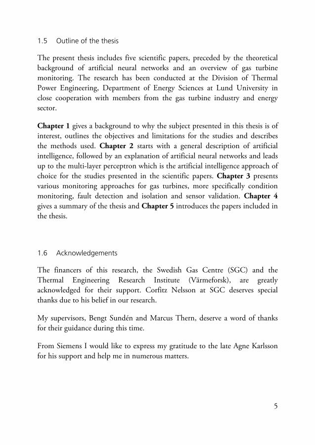
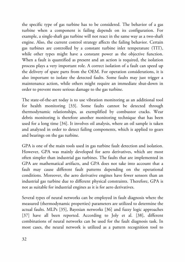
Figure 2.1: The two approaches of AI. [10]

Today, artificial intelligence exists in many shapes and forms and is employed for a large variety of tasks in numerous areas, including speech and handwriting recognition, data mining, medical diagnosis, game playing, robotics and logistics planning. Other applications that many people come into contact with on a daily basis are e-mail spam filtering and Internet search engines.

The remainder of this chapter is dedicated to artificial neural networks, as this data modeling tool was used throughout the research described in the scientific papers. The choice of a suitable AI approach for a given task generally requires much trial-and-error work and the decision was in the present case taken to rely on previous research at the department, which demonstrated that ANN was a good candidate for e.g. simulation, fault diagnosis and sensor validation of heat- and power plants. [11, 12]

AI

Systems that think and act like humans

Fram

ewor

kA

ppro

ach

NeurologyPsychology

PhysicsEngineeringFi

eld

Goa

l Carry out a task withthe best efficiency

Symbolic models- KBS

Connectionist models - ANN

Study of thecognitive processes

Systems that thinkand act rationally

11

2.1 Artificial neural network

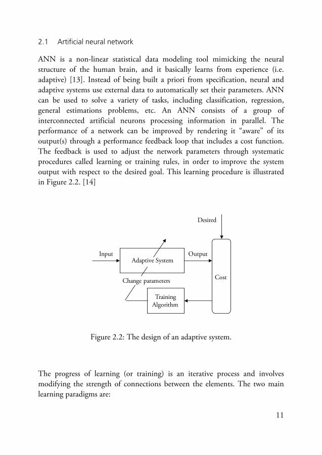
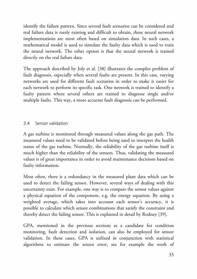
ANN is a non-linear statistical data modeling tool mimicking the neural structure of the human brain, and it basically learns from experience (i.e. adaptive) [13]. Instead of being built a priori from specification, neural and adaptive systems use external data to automatically set their parameters. ANN can be used to solve a variety of tasks, including classification, regression, general estimations problems, etc. An ANN consists of a group of interconnected artificial neurons processing information in parallel. The performance of a network can be improved by rendering it “aware” of its output(s) through a performance feedback loop that includes a cost function. The feedback is used to adjust the network parameters through systematic procedures called learning or training rules, in order to improve the system output with respect to the desired goal. This learning procedure is illustrated in Figure 2.2. [14]

Figure 2.2: The design of an adaptive system.

The progress of learning (or training) is an iterative process and involves modifying the strength of connections between the elements. The two main learning paradigms are:

Adaptive SystemInput Output

Cost

TrainingAlgorithm

Desired

Change parameters

12

• Supervised learning, in which both inputs and desired outputs are known. This means that the network can measure its predictive performance for given inputs.

• Unsupervised learning, in which the targets are unknown and the ANN has to find the underlying relationships within the data set by itself, and build clusters of data. [15]

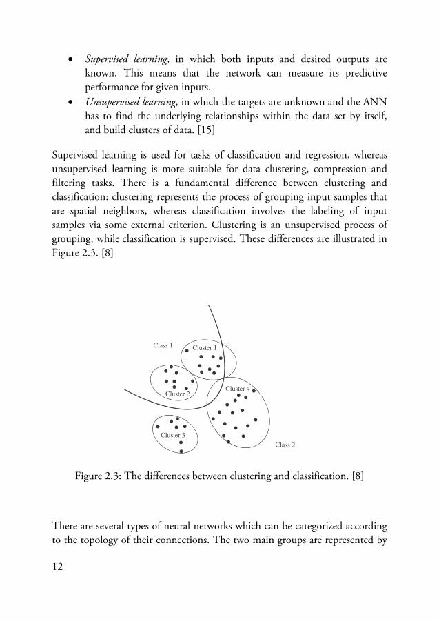
Supervised learning is used for tasks of classification and regression, whereas unsupervised learning is more suitable for data clustering, compression and filtering tasks. There is a fundamental difference between clustering and classification: clustering represents the process of grouping input samples that are spatial neighbors, whereas classification involves the labeling of input samples via some external criterion. Clustering is an unsupervised process of grouping, while classification is supervised. These differences are illustrated in Figure 2.3. [8]

Figure 2.3: The differences between clustering and classification. [8]

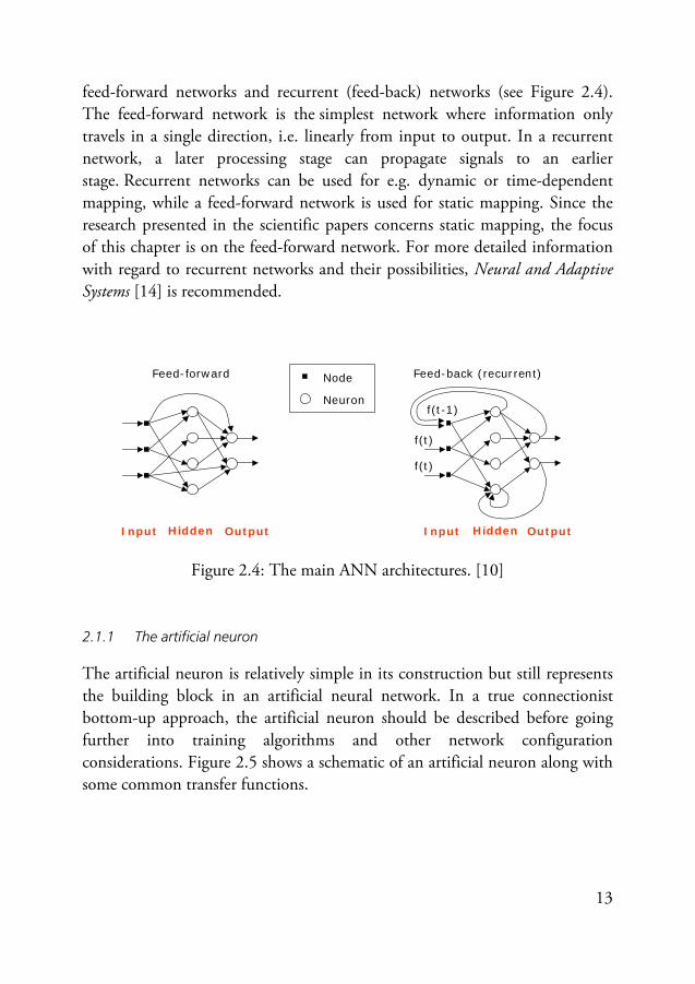
There are several types of neural networks which can be categorized according to the topology of their connections. The two main groups are represented by

13

feed-forward networks and recurrent (feed-back) networks (see Figure 2.4). The feed-forward network is the simplest network where information only travels in a single direction, i.e. linearly from input to output. In a recurrent network, a later processing stage can propagate signals to an earlier stage. Recurrent networks can be used for e.g. dynamic or time-dependent mapping, while a feed-forward network is used for static mapping. Since the research presented in the scientific papers concerns static mapping, the focus of this chapter is on the feed-forward network. For more detailed information with regard to recurrent networks and their possibilities, Neural and Adaptive Systems [14] is recommended.

Figure 2.4: The main ANN architectures. [10]

2.1.1 The artificial neuron

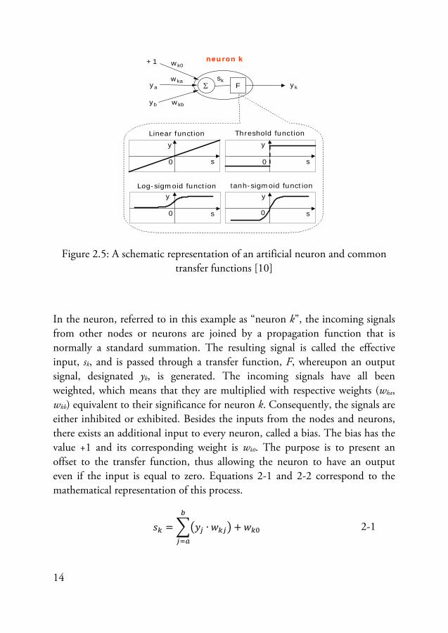
The artificial neuron is relatively simple in its construction but still represents the building block in an artificial neural network. In a true connectionist bottom-up approach, the artificial neuron should be described before going further into training algorithms and other network configuration considerations. Figure 2.5 shows a schematic of an artificial neuron along with some common transfer functions.

Feed-forward

Input OutputHidden

Feed-back (recurrent)

f(t)

f(t-1)

f(t)

Input OutputHidden

Node

Neuron

14

Figure 2.5: A schematic representation of an artificial neuron and common transfer functions [10]

In the neuron, referred to in this example as “neuron k”, the incoming signals from other nodes or neurons are joined by a propagation function that is normally a standard summation. The resulting signal is called the effective input, sk, and is passed through a transfer function, F, whereupon an output signal, designated yk, is generated. The incoming signals have all been weighted, which means that they are multiplied with respective weights (wka, wkb) equivalent to their significance for neuron k. Consequently, the signals are either inhibited or exhibited. Besides the inputs from the nodes and neurons, there exists an additional input to every neuron, called a bias. The bias has the value +1 and its corresponding weight is wk0. The purpose is to present an offset to the transfer function, thus allowing the neuron to have an output even if the input is equal to zero. Equations 2-1 and 2-2 correspond to the mathematical representation of this process.

𝑠𝑘 = ��𝑦𝑗 ∙ 𝑤𝑘𝑗� + 𝑤𝑘0

𝑏

𝑗=𝑎

2-1

wk0

wkb

ykFΣya

yb

sk

neuron k

Linear function Threshold function

Log-sigmoid function tanh-sigmoid function

y

0 0 s

y

y

0

y

0

+1

wka

s

s

s

15

𝑦𝑘 = 𝐹(𝑠𝑘) 2-2

2.1.2 The single-layer feed-forward network

The single-layer network is defined in the sense that there is only one layer with artificial neurons. The simplest single-layer feed-forward network is called the Perceptron and has only a single neuron. The Perceptron convergence algorithm uses supervised training in order to update the connection strengths (weights). As explained earlier, in supervised training, the desired outputs are known and employed in a cost function to calculate an error that is then used by the training algorithm to update the system. Presuming that the desired outputs of the data set are known, an error can be defined as the difference between this desired output, also known as target, and the output calculated by the ANN:

𝑒(𝑛) = 𝑑(𝑛) − 𝑦(𝑛) 2-3

However, prior to the calculation of errors, the weights have to be assigned random starting values. When the weights have received their starting values, the first input vector, x in Equation 2-4, is presented to the network, which then generates an output. This output is subsequently used to calculate the first error, employed in the perceptron training algorithm to calculate the next set of weights, i.e. the new training vector (according to Equation 2-4). When the weights have been updated, a new input vector is presented to the network and the whole procedure is repeated until the iteration receives the order to stop. The learning rate factor, η, varies between 0 and +1.

𝒘(𝑛 + 1) = 𝒘(𝑛) + 𝜂 ∙ 𝑒(𝑛) ∙ 𝒙(𝑛) 2-4

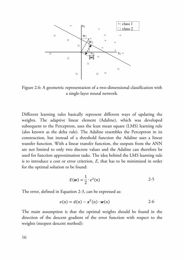
The Perceptron uses a threshold transfer function rendering it suitable for simple classification tasks. The graphical representation of a two-dimensional (i.e. two inputs) classification is illustrated in Figure 2.6, where the weights determine the slope of the line and the bias determines the distance of the line from its origin, i.e. offset.

16

x2

x1

w2

w1

w0w−

+: class 1 �: class 2

Figure 2.6: A geometric representation of a two-dimensional classification with a single-layer neural network.

Different learning rules basically represent different ways of updating the weights. The adaptive linear element (Adaline), which was developed subsequent to the Perceptron, uses the least mean square (LMS) learning rule (also known as the delta rule). The Adaline resembles the Perceptron in its construction, but instead of a threshold function the Adaline uses a linear transfer function. With a linear transfer function, the outputs from the ANN are not limited to only two discrete values and the Adaline can therefore be used for function approximation tasks. The idea behind the LMS learning rule is to introduce a cost or error criterion, E, that has to be minimized in order for the optimal solution to be found:

𝐸(𝒘) =12∙ 𝑒2(𝑛) 2-5

The error, defined in Equation 2-3, can be expressed as:

𝑒(𝑛) = 𝑑(𝑛) − 𝒙𝑇(𝑛) ∙ 𝒘(𝑛) 2-6

The main assumption is that the optimal weights should be found in the direction of the descent gradient of the error function with respect to the weights (steepest descent method):

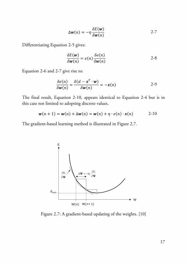
17

∆𝒘(𝑛) = −𝜂𝛿𝐸(𝒘)𝛿𝒘(𝑛) 2-7

Differentiating Equation 2-5 gives:

𝛿𝐸(𝒘)𝛿𝒘(𝑛) = 𝑒(𝑛)

𝛿𝑒(𝑛)𝛿𝒘(𝑛) 2-8

Equation 2-6 and 2-7 give rise to:

𝛿𝑒(𝑛)𝛿𝒘(𝑛) =

𝛿(𝑑 − 𝒙𝑇 ∙ 𝒘)𝛿𝒘(𝑛) = −𝒙(𝑛) 2-9

The final result, Equation 2-10, appears identical to Equation 2-4 but is in this case not limited to adopting discrete values.

𝒘(𝑛 + 1) = 𝒘(𝑛) + ∆𝒘(𝑛) = 𝒘(𝑛) + 𝜂 ∙ 𝑒(𝑛) ∙ 𝒙(𝑛) 2-10

The gradient-based learning method is illustrated in Figure 2.7.

Figure 2.7: A gradient-based updating of the weights. [10]

E

WW(n) W(n+1)

Emin

WW

∂∂

⋅η−=∆E

W∂∂E

18

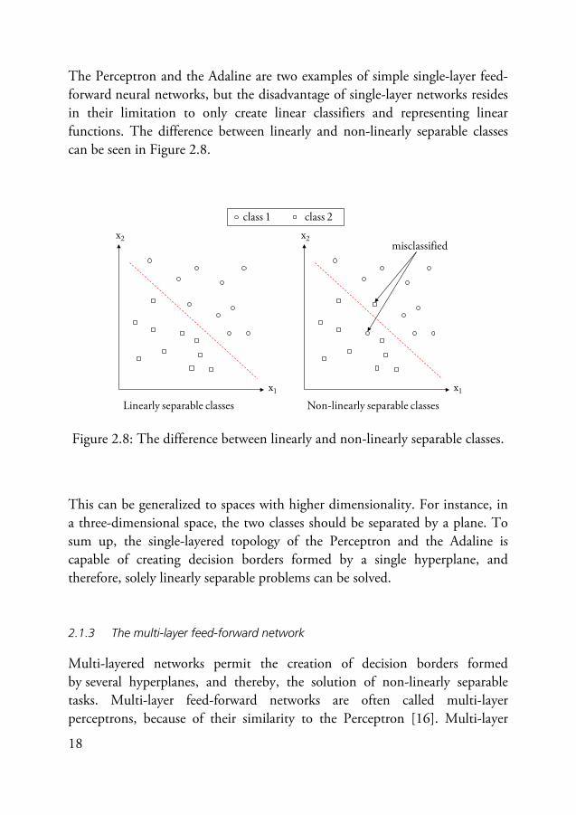
The Perceptron and the Adaline are two examples of simple single-layer feed-forward neural networks, but the disadvantage of single-layer networks resides in their limitation to only create linear classifiers and representing linear functions. The difference between linearly and non-linearly separable classes can be seen in Figure 2.8.

Figure 2.8: The difference between linearly and non-linearly separable classes.

This can be generalized to spaces with higher dimensionality. For instance, in a three-dimensional space, the two classes should be separated by a plane. To sum up, the single-layered topology of the Perceptron and the Adaline is capable of creating decision borders formed by a single hyperplane, and therefore, solely linearly separable problems can be solved.

2.1.3 The multi-layer feed-forward network

Multi-layered networks permit the creation of decision borders formed by several hyperplanes, and thereby, the solution of non-linearly separable tasks. Multi-layer feed-forward networks are often called multi-layer perceptrons, because of their similarity to the Perceptron [16]. Multi-layer

x2

x1

class 1 class 2x2

x1

misclassified

Linearly separable classes Non-linearly separable classes

19

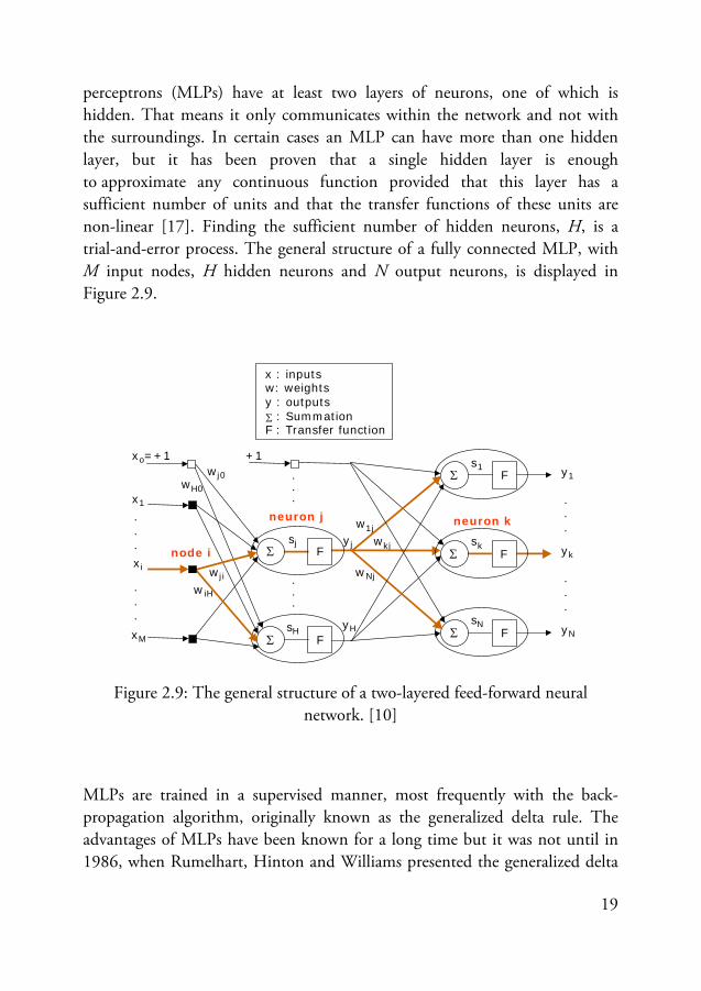
perceptrons (MLPs) have at least two layers of neurons, one of which is hidden. That means it only communicates within the network and not with the surroundings. In certain cases an MLP can have more than one hidden layer, but it has been proven that a single hidden layer is enough to approximate any continuous function provided that this layer has a sufficient number of units and that the transfer functions of these units are non-linear [17]. Finding the sufficient number of hidden neurons, H, is a trial-and-error process. The general structure of a fully connected MLP, with M input nodes, H hidden neurons and N output neurons, is displayed in Figure 2.9.

w kj w Nj

x : inputs w: weights y : outputs Σ : Summation F : Transfer function

y H

x o =+1

x M

w j0

neuron j

w H0

neuron k y j y k F Σ

s k F Σ s j

F Σ s H

x 1 . . .

.

.

.

.

.

.

.

.

.

.

.

.

+1

w 1j

x i . . .

w ji w iH

y 1 F Σ s 1

y N F Σ s N

node i

Figure 2.9: The general structure of a two-layered feed-forward neural network. [10]

MLPs are trained in a supervised manner, most frequently with the back-propagation algorithm, originally known as the generalized delta rule. The advantages of MLPs have been known for a long time but it was not until in 1986, when Rumelhart, Hinton and Williams presented the generalized delta

20

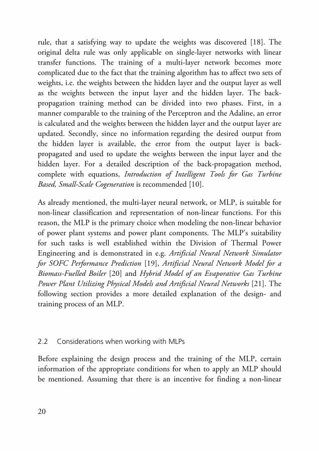
rule, that a satisfying way to update the weights was discovered [18]. The original delta rule was only applicable on single-layer networks with linear transfer functions. The training of a multi-layer network becomes more complicated due to the fact that the training algorithm has to affect two sets of weights, i.e. the weights between the hidden layer and the output layer as well as the weights between the input layer and the hidden layer. The back-propagation training method can be divided into two phases. First, in a manner comparable to the training of the Perceptron and the Adaline, an error is calculated and the weights between the hidden layer and the output layer are updated. Secondly, since no information regarding the desired output from the hidden layer is available, the error from the output layer is back-propagated and used to update the weights between the input layer and the hidden layer. For a detailed description of the back-propagation method, complete with equations, Introduction of Intelligent Tools for Gas Turbine Based, Small-Scale Cogeneration is recommended [10].

As already mentioned, the multi-layer neural network, or MLP, is suitable for non-linear classification and representation of non-linear functions. For this reason, the MLP is the primary choice when modeling the non-linear behavior of power plant systems and power plant components. The MLP’s suitability for such tasks is well established within the Division of Thermal Power Engineering and is demonstrated in e.g. Artificial Neural Network Simulator for SOFC Performance Prediction [19], Artificial Neural Network Model for a Biomass-Fuelled Boiler [20] and Hybrid Model of an Evaporative Gas Turbine Power Plant Utilizing Physical Models and Artificial Neural Networks [21]. The following section provides a more detailed explanation of the design- and training process of an MLP.

2.2 Considerations when working with MLPs

Before explaining the design process and the training of the MLP, certain information of the appropriate conditions for when to apply an MLP should be mentioned. Assuming that there is an incentive for finding a non-linear

21

relation between numerical data (i.e. creating a model), some basic considerations include the following:

• Since ANN is a statistical data modeling tool, a set of examples that are appropriately distributed over the input space and in sufficient numbers, must be available.

• The need for a non-linear model should be examined, since the design of a linear model is much simpler and faster. This can e.g. be done by first trying a linear model and, if it is found to be too inaccurate despite that all relevant factors are presented in the inputs, one can resort to a non-linear model.

• Finally, in cases where enough samples are available and a non-linear behavior is confirmed, one should consider whether neural networks should be employed instead of e.g. polynomials. This is a matter of how many variables the system to be modeled has, since the number of parameters in the first connection layer of a neural network increases linearly with the number of inputs, whereas it increases exponentially for polynomial approximations. Empirically, neural networks are advantageous when the number of inputs is equal to or exceeds three. [22]

2.2.1 Setup and training

Once the use of neural networks for the non-linear modeling (regression) of a system has been established, certain network specifics have to be decided on, such as these criteria:

• Number of hidden layers • Number of neurons in hidden layers • Transfer functions in neurons • Error criteria • Training algorithm • Stop criteria • Initial values of weights

22

No attempt is made to explain everything in detail. The objective is rather to provide a general overview of the decisions one might face when designing an MLP.

The number of hidden layers is decided based on trial-and-error. But one hidden layer is enough to approximate any continuous function, as long as the number of neurons in this hidden layer is sufficient. Additional hidden layers are seldom required for regression tasks while it might be useful for other tasks. [14]

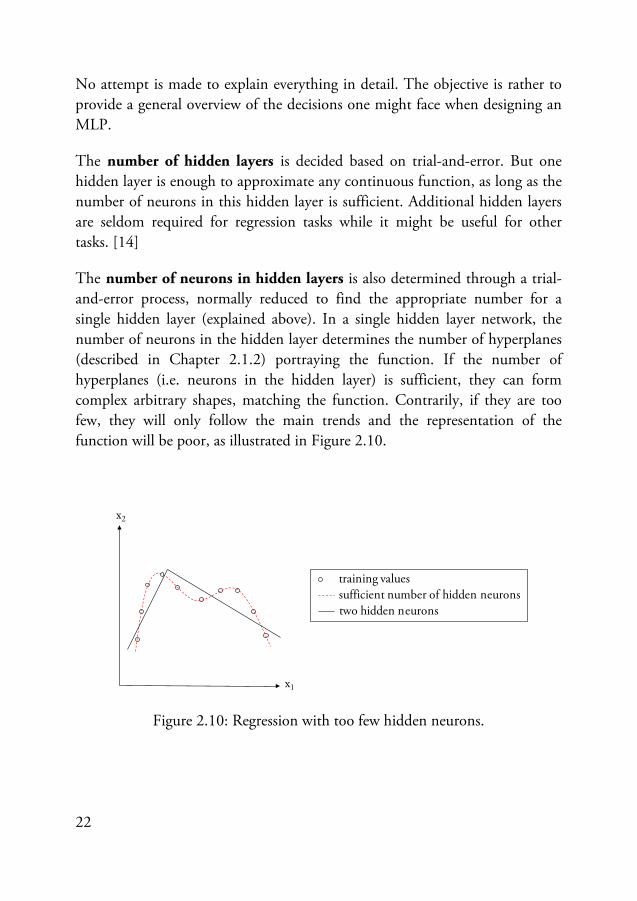
The number of neurons in hidden layers is also determined through a trial-and-error process, normally reduced to find the appropriate number for a single hidden layer (explained above). In a single hidden layer network, the number of neurons in the hidden layer determines the number of hyperplanes (described in Chapter 2.1.2) portraying the function. If the number of hyperplanes (i.e. neurons in the hidden layer) is sufficient, they can form complex arbitrary shapes, matching the function. Contrarily, if they are too few, they will only follow the main trends and the representation of the function will be poor, as illustrated in Figure 2.10.

Figure 2.10: Regression with too few hidden neurons.

x2

x1

training values sufficient number of hidden neuronstwo hidden neurons

23

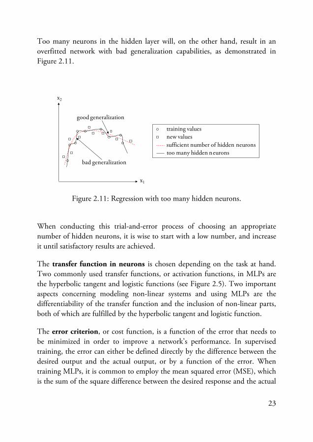
Too many neurons in the hidden layer will, on the other hand, result in an overfitted network with bad generalization capabilities, as demonstrated in Figure 2.11.

Figure 2.11: Regression with too many hidden neurons.

When conducting this trial-and-error process of choosing an appropriate number of hidden neurons, it is wise to start with a low number, and increase it until satisfactory results are achieved.

The transfer function in neurons is chosen depending on the task at hand. Two commonly used transfer functions, or activation functions, in MLPs are the hyperbolic tangent and logistic functions (see Figure 2.5). Two important aspects concerning modeling non-linear systems and using MLPs are the differentiability of the transfer function and the inclusion of non-linear parts, both of which are fulfilled by the hyperbolic tangent and logistic function.

The error criterion, or cost function, is a function of the error that needs to be minimized in order to improve a network’s performance. In supervised training, the error can either be defined directly by the difference between the desired output and the actual output, or by a function of the error. When training MLPs, it is common to employ the mean squared error (MSE), which is the sum of the square difference between the desired response and the actual

x2

x1

training values

sufficient number of hidden neuronstoo many hidden neurons

new values

bad generalization

good generalization

24

output. The MSE is minimized by changing the weights according to the training algorithm and, if the MSE reaches zero, the network output matches the desired outputs. [14]

The training algorithm, most commonly used together with MLPs, is the back-propagation training algorithm, also known as the generalized delta rule (see Chapter 2.1.2). The learning is based on an error criterion that is minimized with respect to the weights in the network. The challenge, as compared to the training of a single-layer network, is that no information concerning target values can be obtained from the neurons in the hidden layer. In other words, if an output unit produces an incorrect response when the network is presented with an input vector, there is no way of knowing which of the hidden units is responsible. Consequently, it is impossible to know which weight to adjust, and by how much. The solution is differentiable error criterion (or error function) and activation functions, formulated by Bishop as: “If we consider a network with differentiable activation functions, then the activations of the output units become differentiable functions of both the input variables, and the weights and biases. If we define an error function which is a differentiable function of the network outputs, then the error is itself a differentiable function of the weights. We can therefore evaluate the derivatives of the error with respect to the weights, and these derivatives can then be used to find weight values which minimize the error function, by using e.g. gradient descent. The algorithm for evaluating the derivatives of the error function is known as back-propagation since it corresponds to a propagation of errors backwards through the network.” [23]

The stop criteria can be used to avoid overtraining through the application of a cross-validation method. The cross-validation method involves measuring the network’s performance during training and, if any incentive is given, stop the training before the maximum number of iterations (epochs) is reached. This is done by splitting the data set into two parts, one training data set and one cross-validation data set. The training data set is used to calculate the errors and is thereby a part in the process of updating the weights. The cross-validation data set is not directly used in the training, but continuously verifies the networks performance with independent patterns during the training procedure. If the error (e.g. MSE) based on the cross-validation data set starts

25

to increase, as the error based on the training data set continues to decrease, it is an indication of overtraining.

The initial values of weights are normally set by randomization since no analytical solution is available. Nevertheless, certain aspects are worth considering. The initial values should be in a range so that the input to the transfer function is kept out of the saturated region. It is also of interest that the neurons learn at the same rate, which can be accomplished by providing them with equal starting conditions. [14]

For more information on any of these steps, Neural Networks for Pattern Recognition [23] and Neural and Adaptive Systems [14] are recommended.

2.2.2 Data management

Since data is the number one prerequisite when using a data-driven method such as ANN, the final part of Chapter 2.2 contains a list of items regarding data management:

• Filtering • Sizing the sets • Normalization

Filtering of the data is important in order to avoid that any corrupt data, such as outliers, is used in the training process. If such data is included in the training, it might have a negative effect on the overall predictive performance of the network.

Sizing the sets appropriately is essential in order to achieve the best results. The most important data set is the training data set where it is crucial that it contains enough well-distributed patterns. A rule of thumb is that the number of training patterns should be ten times larger than the number of weights in the network [13]. The purpose of the cross-validation data set is to test the performance of the network during training and it is normally much smaller than the training data set. The last set, the test data set, has not been mentioned until now, and is used to examine a network’s performance with

26

unseen data after completion of the training. A normal distribution between the data sets can e.g. be 60-25-15 (training, cross-validation and test).

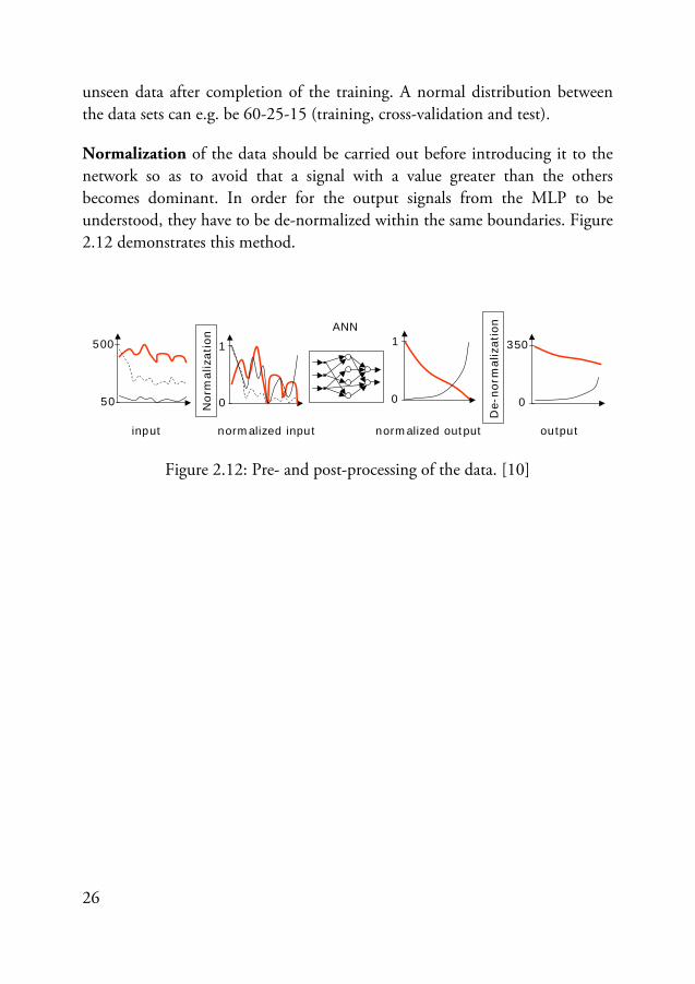
Normalization of the data should be carried out before introducing it to the network so as to avoid that a signal with a value greater than the others becomes dominant. In order for the output signals from the MLP to be understood, they have to be de-normalized within the same boundaries. Figure 2.12 demonstrates this method.

Figure 2.12: Pre- and post-processing of the data. [10]

ANN

Nor

mal

izat

ion

1

0

500

50

De-

norm

aliz

atio

n

350

0

1

0

input normalized input normalized output output

27

3 Gas turbine monitoring

This chapter is an introduction to the research field of gas turbine monitoring, explaining some different approaches within the subareas. The subareas for this work are identified as condition monitoring, sensor validation and fault diagnosis. Condition monitoring is the process of monitoring one or several parameters of the condition in a piece of machinery, such that a significant change is indicative of a developing failure. This allows intervention in the early stages of deterioration, which is generally much more cost-effective than letting the machinery fail completely. Sensor validation is the process of monitoring sensor accuracy, detecting and isolating failing sensors and recovering sensor values. The goal is to avoid forced outages due to sensor faults. Fault diagnosis is the process of detecting and isolating faults occurring in the machinery with the same goal as with condition monitoring. In addition to early intervention, the isolation of faults acts as an aid in the maintenance process.

3.1 Background

Monitoring is a general term for which the main goal is to detect different types of performance deterioration, such as degradation, machine faults and sensor faults. Degradation and machine faults are hardware errors that indicate the health status of the gas turbine. The following conditions are typical of gas turbine deterioration [24]:

28

• Fouling • Variable inlet guide vane and variable stator vane problems • Hot end damage • Tip rubs • Vibration • Seal wear and damage • Foreign object damage and domestic object damage • Erosion • Corrosion • Control system malfunction

Any of these conditions will cause a change in the performance of a gas turbine. Fouling is a temporary deterioration that can be restored by compressor cleaning while for instance hot end damage and tip rubs require a complete overhaul of the gas turbine. To quantify the deterioration in a gas turbine, a mathematical model called baseline of the gas turbine in a healthy and new condition is used. By comparing the baseline values against the actual measured values from the gas turbine, a quantification of the current deterioration can be performed. An accurate baseline model of the gas turbine is thereby crucial for the success of health monitoring systems.

The deterioration effect will progressively worsen with increasing operating time. The rate of deterioration can be divided into three main types of failure common to all machines: time-dependent, delayed time dependent and instantaneous failures [25]. The latter will occur without any warning, thereby impossible for any monitoring system to detect. The delayed time-dependent failure is one where the deterioration is not detectable until a certain point in time. This type of failure will degrade an engine in a well-defined rate. The two time-dependent failure trends are candidates for a monitoring system.

The quality of the quantification of the current performance deterioration at the current time is dependent on accurate sensor values. Corrupted sensor values might indicate performance deterioration and may contribute to faulty decisions with regard to maintenance, which in turn will affect the reliability of the power plant negatively. Most often, hardware such as compressors and turbines are much more reliable than the sensor and control system [26].

29

Therefore, before using the measured data from the gas turbine, data filtering and sensor validation should be applied to it.

Engine health monitoring systems consist of several different methods, of which gas path analysis (GPA), presented by Urban in 1969 [27], is one of the most famous. GPA, as introduced by Urban, is a linear differential method where changes in the measured parameters are used to evaluate the deteriorated components. Later on, GPA was combined with the optimal state estimation method called a Kalman filter to come to terms with uncertainties in the measurements. Versions of the GPA, where statistical algorithms have been used to estimate sensor errors, are presented in for instance [28] and [29].

All gas turbines and power plants are equipped with numerous sensors measuring their performance during operation. The primary reason for this is to supply various control systems with information. Basically, control systems use incoming, measured data to correct a signal for a control device with the aim of reaching a set point for a given parameter. This ensures the correct operation of the plant or component in all operating conditions, including transient conditions. There are several “control loops” in a power plant which control everything from component-specific parameters through process parameters to main plant parameters. Besides being used for the control of the power plant, the stream of data is employed to monitor the equipment and generate warnings, alarms and even induce complete shut-downs of the operation if needed. The development of data-driven monitoring tools, such as ANN-based condition monitoring and sensor validation, is made possible much on account of this generated operational data.

3.2 Condition monitoring

The main goal of condition monitoring is to optimize the maintenance cost of a power plant. The three principle maintenance strategies include:

• Run-to-failure: the plant is basically operated until it breaks down. • Preventive: a planned maintenance service schedule is applied.

30

• Predictive (condition-based maintenance): the maintenance schedule is planned according to the actual condition of the plant or component.

The run-to-failure method has several drawbacks. First, a failing component may cause failure in other components, which can lead to the total break-down of the gas turbine. Another disadvantage is that the failing component might cause a shut-down during a critical time where the power is needed the most. Preventive maintenance has been the main method for a long time and is based on regular intervals. However, this method is also accompanied by certain drawbacks. For instance, failures do not occur regularly and might take place unexpectedly in between the overhauls. Also, this method will cause unnecessary overhauls of the components, resulting in time-consuming maintenance and major profit losses for the power plant owners. Predictive maintenance on the other hand is based on the actual condition, hence the name condition monitoring, and maintenance can be planned at an optimal time, which would generate the highest profit for the power plant owners.

Condition monitoring addresses additional challenges, since it requires a health monitoring system which, at any point, can convey the health status of the plant. Practically, this is done by comparing the actual performance against a mathematical model of the gas turbine representing the performance in a healthy status. Differences between the actual performance and the baseline model can be interpreted as performance deterioration. The “health” of a gas turbine is normally expressed as the efficiency of the components; parameters that cannot be measured directly. Instead, the health factors have to be calculated through measurable values, e.g. temperatures and pressures along the gas path of the engine.

GPA addresses this problem by relating the changes in the measured parameters to changes in the health parameters, and since GPA is a differential method, changes in the health parameters are monitored rather than absolute values. The literature on GPA approaches for monitoring is extensive and the following references represent the pioneering work [25, 27, 30].

Another monitoring approach consists in constructing a purely mathematical model, based on physical laws such as heat and mass balances together with

31

the characteristics of the components. These models can be made very accurate. However, they require sensitive information about all components which most often is highly confidential. The original equipment manufacturers (OEMs) use these models in the design phase but are reluctant to supplying them to the operators due to the sensitive information contained within the models. As another drawback, the method generally requires more input than is normally available for an “on-site” engine. Furthermore, the effort to build such a model is normally too costly for it to be considered a practical solution.

Data-driven models have emerged in the engineering community during the last 10-20 years [31]. In a data-driven model, the baseline model is developed directly from the measured data without the addition of any physical principles. Data corresponding to a healthy operation is used to train the data-driven model. There are several methods to choose between, such as radial basis function networks, feed-forward multi-layer perceptrons, polynomials etc. However, for high-dimensional systems (with more than three input parameters), the multi-layer perceptron method is considered the most attractive. This is the only data-driven method that scales linearly with the dimension, making it highly appropriate for high-dimensional modeling.

Since the 1980s, a mathematical theory for feed-forward multi-layer perceptrons has existed, which shows that the MLP is a universal approximator [17, 32]. However, the building of the model is a somewhat complex problem and today’s research is still on trial even though some guidelines are available. Much of the current research work is focused on demonstrating different applications and methodologies to apply the MLP. Data-driven modeling offers a cost-effective approach to condition monitoring, since all that is needed to build the monitoring model is data from the gas turbine.

3.3 Fault detection and isolation

Fault detection and isolation is the process of detecting a faulty data pattern, and then isolating it as a specific fault. This is not an easy task in a gas turbine, due to high intercorrelation between the components. The control as well as

32

the specific type of gas turbine has to be considered. The behavior of a gas turbine when a component is failing depends on its configuration. For example, a single-shaft gas turbine will not react in the same way as a two-shaft engine. Also, the current control strategy affects the failing behavior. Certain gas turbines are controlled by a constant turbine inlet temperature (TIT), while other types might have a constant power as the objective function. When a fault is quantified as present and an action is required, the isolation process plays a very important role. A correct isolation of a fault can speed up the delivery of spare parts from the OEM. For operation considerations, it is also important to isolate the detected faults. Some faults may just trigger a maintenance action, while others might require an immediate shut-down in order to prevent more serious damage to the gas turbine.

The state-of-the-art today is to use vibration monitoring as an additional tool for health monitoring [33]. Some faults cannot be detected through thermodynamic relationships, as exemplified by combustor cracks. Wear debris monitoring is therefore another monitoring technique that has been used for a long time [34]. It involves oil analysis, where an oil sample is taken and analyzed in order to detect failing components, which is applied to gears and bearings on the gas turbine.

GPA is one of the main tools used in gas turbine fault detection and isolation. However, GPA was mainly developed for aero derivatives, which are most often simpler than industrial gas turbines. The faults that are implemented in GPA are mathematical artifacts, and GPA does not take into account that a fault may cause different fault patterns depending on the operational conditions. Moreover, the aero derivative engines have fewer sensors than an industrial gas turbine due to different physical constraints. Therefore, GPA is not as suitable for industrial engines as it is for aero derivatives.

Several types of neural networks can be employed in fault diagnosis where the measured (thermodynamic properties) parameters are utilized to determine the actual faults. MLPs [35], Bayesian networks [36] and fuzzy logic approaches [37] have all been reported. According to Joly et al. [38], different combinations of neural networks can be used for the fault diagnosis task. In most cases, the neural network is utilized as a pattern recognition tool to

33

identify the failure pattern. Since several fault scenarios can be considered and real failure data is rarely existing and difficult to obtain, these neural network implementations are most often based on simulation data. In such cases, a mathematical model is used to simulate the faulty data which is used to train the neural network. The other option is that the neural network is trained directly on the real failure data.

The approach described by Joly et al. [38] illustrates the complex problem of fault diagnosis, especially when several faults are present. In this case, varying networks are used for different fault scenarios in order to make it easier for each network to perform its specific task. One network is trained to identify a faulty pattern where several others are trained to diagnose single and/or multiple faults. This way, a more accurate fault diagnosis can be performed.

3.4 Sensor validation

A gas turbine is monitored through measured values along the gas path. The measured values need to be validated before being used to interpret the health status of the gas turbine. Normally, the reliability of the gas turbine itself is much higher than the reliability of the sensors. Thus, validating the measured values is of great importance in order to avoid maintenance decisions based on faulty information.

Most often, there is a redundancy in the measured plant data which can be used to detect the failing sensor. However, several ways of dealing with this uncertainty exist. For example, one way is to compare the sensor values against a physical equation of the component, e.g. the energy equation. By using a weighted average, which takes into account each sensor’s accuracy, it is possible to calculate which sensor combinations that satisfy the constraint and thereby detect the failing sensor. This is explained in detail by Rodney [39].

GPA, mentioned in the previous sections as a candidate for condition monitoring, fault detection and isolation, can also be employed for sensor validation. In these cases, GPA is utilized in conjunction with statistical algorithms to estimate the sensor error, see for example the work of

34

Lunderstaedt et al. [28] and Doel et al. [29]. The weighted least square techniques applied to the GPA have been shown in [29, 40, 41].

Neural networks provide another approach to sensor validation, which has been extensively studied. Several types of neural networks have been applied to sensor validation of power plants in numerous ways. Sensor validation has been demonstrated through the Kohonen Map, the feed-forward MLP and the auto-associative neural network [42, 43]. Commonly, the neural network is trained with a data set either generated by a simulation program, as shown by Ogaji et al. [43], or by operational data from the system (gas turbine). It is possible to make a distinction here, between a case where the neural network is developed with simulated data and one where it is developed with real operational data. For the former, the neural network is used since it provides a simpler way of implementation for real-time monitoring than the simulation program itself. For the latter, where the neural network is developed from real data, the situation is rather different. Most often, there is no mathematical model available; only measured data from the system (gas turbine). The network is then used to build the model directly from this data.

The most common implementation of a neural network is through the auto-associative neural network (AANN), a so-called identity mapper, where the network is trained to reproduce the input values to the outputs. When a faulty sensor is present in the input data, the network predicts a more accurate value since the correlations between the parameters are learned by the network in the learning session. The network output is therefore a more reliable value than the input value itself. An AANN can mainly be configured in two different ways, i.e. with one or three hidden layers. When an AANN is configured with one hidden layer, the correlations between the parameters are learned during the training session. When three hidden layers are used, a certain compression is also applied by a so-called bottle-neck layer which consists of fewer neurons than the input/output layers. Two of the first publications to have introduced neural networks for sensor validation are reported by Kramer [44, 45]. Since then applications have been numerous [26, 46, 47].

35

The building of mathematical models through physical laws is a complicated process, especially for highly interconnected systems with losses (turbulence etc.) which are difficult to model in an accurate way. In this aspect, neural networks provide the option to build the monitoring models directly from the operational data, thus presenting a cost-effective option for sensor validation. Neural networks provide the capability of using high dimensional and nonlinear data in an efficient manner, characteristics which are always hard to simulate with analytical models. Another aspect worth mentioning is that sensor accuracy etc. is directly included in the neural network. This results in robust models which are insensitive to small input errors that are common in real measured data.

37

4 Concluding remarks

Data-driven modeling has emerged during the last decades as an alternative to physical simulation for monitoring purposes. One of the main reasons is the sophisticated data acquisition systems introduced during the last years, which are used to store measured data from power plants. The data itself is not worth much if it is not analyzed. However, plant operators do not have access to the detailed component characteristics needed for accurate physical modeling. Thus, using the saved data provides an efficient and cost-effective approach for the modeling.

The main goal of this thesis has been to evaluate ANN as a data-driven modeling approach aimed at fault detection, degradation estimation and sensor validation of gas turbines. By assessing several gas turbines with varying characteristics in terms of off-design behavior, the generic capabilities of the approach were validated. Another goal was to determine the economical impact caused by degradation in gas turbines.

A new technology is always met with a certain amount of skepticism, until it is proven reliable and trustworthy. In this case, the users of the models are the plant operators which normally have only limited knowledge of the gas turbine. A graphical user interface was developed and presented to the plant operators, demonstrating the usability of the ANN model. In practice, the user interface showed that the ANN monitoring model could be employed without any knowledge from the user side, which is an advantage for practical implementation. Moreover, the user interface could be operated both offline for training as well as online for real-time monitoring. Online monitoring by

38

the ANN models demonstrated that, as long as the ANN model predictions and real measurements were similar, the operation continued without faults. If any deviations between the model and the measurements were observed, an investigation of the underlying reason was needed. Advantageously, no effort was required until the detection of a faulty behavior. In this way, unnecessary data analysis could be avoided.

The deregulation of the electricity market has resulted in new challenges for the power producers. Combined power plants, which previously were only operated in base load, nowadays function more often in part load, caused by for instance the introduction of wind power to the market. More sophisticated monitoring systems are required, with the possibility of being used in real time to detect failures and abnormal behavior of the gas turbine as early as possible.

This thesis has shown the feasibility of introducing ANNs as a candidate for data driven modeling for gas turbine monitoring. It was demonstrated that accurate monitoring models could be developed by using measured data, without detailed information about the gas turbine. This renders it possible for plant owners to develop their own monitoring systems for their specific plants.

39

5 Summary of Papers

Paper I. Development and multi-utility of an ANN model for an industrial gas turbine. Journal of Applied Energy, Vol. 86, Issue 1, pp. 9-17, January 2009.

This paper describes the investigation of MLP capacities for gas turbine modeling using operational data from a Siemens SGT-600 machine. Operational data was primarily chosen to evaluate the possibilities of creating an accurate performance-predicting ANN model representing an actual machine. Besides creating a precise model, various real-life aspects, associated with the modeling of an actual machine, where examined. These real-life aspects included everything from data acquisition and filtering to specific operational conditions, such as anti-icing operation.

This study demonstrates that the use of ANN rendered it possible to create tailor-made models, with very high prediction accuracies, using operational data for specific gas turbines. Together with the developed user-friendly graphical user interface, the model can be employed for offline performance simulation for operation planning or as a tool in the training of new operators. The model also shows potential to be integrated in online condition monitoring.

The author of this thesis carried out everything from the data acquisition and filtering through the training and evaluation of the ANN models to the development of the user interface. Mohsen Assadi was the coordinator of the work and participated in the analysis of the results. Sudipta De helped compile the material into a scientific paper.

40

Paper II. Application of artificial neural network to the condition monitoring and diagnosis of a combined heat and power plant was presented and published at the ECOS conference in Krakow, Poland, in the summer of 2008. Upon recommendation, this paper was later also published in the Journal of Energy, Vol. 35, pp. 1114-1120, 2010.

This paper presents the ANN modeling of several power plant components using operational data. The components included a gas turbine, a heat recovery steam generator, a biomass-fueled boiler and a steam turbine. The possibility of integrating these ANN models in the power plant’s computer system and developing a graphical user interface for realizing online condition monitoring was also investigated.

This study demonstrates that ANN can be advantageously employed for modeling of several different components with high accuracy. Thanks to the limited size of the ANN models, their high computational speed and the transferability into any programming language, the integration and functionality in combination with the power plant’s computer system was successful. Together with the developed graphical user interface, condition monitoring was demonstrated to be an achievable goal.

The author of this thesis carried out everything from the data acquisition to the implementation of the ANN models in the power plant’s computer system as well as the evaluation of the complete online system. Thomas Palmé contributed with fruitful discussions during the course of the investigation.

Paper III. Condition-based maintenance of gas turbines using simulation data and artificial neural network: A demonstration of feasibility was presented and published at AMSE Turbo Expo, Berlin, Germany, in the summer of 2008.

This paper investigates the possibilities of using simulation data, instead of operational data, for ANN modeling of gas turbines in order to overcome the unavailability of data for new gas turbines. This is an attempt at enabling the delivery of an ANN tool, for condition monitoring, together with new gas turbines. Simulation data was produced with Siemens’ own design tool

41

representing their SGT-800 gas turbine. An ANN model was trained with this data and its performance was compared to that of an ANN model trained with operational data.

This study presented limitations since the ANN model that was trained with simulation data was not developed for this specific purpose. However, when eliminating these factors, the congruence between the ANN model trained with simulation data and the one trained with operational data was close to perfect.

The author of this thesis carried out the data acquisition and filtering, the training of the ANN model based on operational data and the comparison of the performances between the two models. The ANN model trained with simulation data was developed by Jaime Arriagada, a former Ph.D. student at the Division of Thermal Power Engineering. Mohsen Assadi was the coordinator of the work and participated in the analysis of the results. Sudipta De helped compile the material into a scientific paper.

Paper IV. A novel approach for gas turbine condition monitoring combining CUSUM technique and artificial neural network was presented and published at AMSE Turbo Expo, Orlando, Florida, USA, in the summer of 2009.

This paper reports on the combination of an artificial neural network and a sequential analysis technique for monitoring of a gas turbine. The performed work was an attempt at eliminating the need for retraining or calibration of the performance-predicting model (in this case the ANN model) as the gas turbine was deteriorated. Another benefit may also be the detection of very small gas turbine anomalies.

In this study, operational data from a Siemens SGT-600 gas turbine was employed for the training of an ANN model, which was subsequently used for the prediction of performance parameters of the gas turbine. Simulated anomalies were introduced on two sets of operational data, acquired one year apart, whereupon this data was compared to corresponding ANN predictions.

42

The cumulative sum (CUSUM) technique was utilized to improve and facilitate the detection of such anomalies in the gas turbine’s performance.

The author of this thesis performed the ANN model training, implementation of the CUSUM algorithm and the analysis of the results. Thomas Palmé carried out the literature review and helped in the writing of the paper. He also participated in the analysis of the results. Magnus Genrup initiated the study.

Paper V. Gas Turbine Sensor Validation through Classification with Artificial Neural Networks was presented and published at the ECOS conference in Foz do Iguaçu, Paraná, Brazil, in the summer of 2009.

This paper presents a method for evaluating sensor accuracy, with the aim of minimizing the need for calibration and at the same time avoiding shut-downs due to sensor faults etc.

The proposed method was based on the training of artificial neural networks as classifiers to recognize sensor drifts. The method was evaluated on two types of gas turbines, i.e. one single-shaft and one twin-shaft machine. The results demonstrated that the method was capable of early detection of sensor drifts for both machine types as well as of an accurate production of soft measurements.

The technical work was equally divided between the author of this thesis and Thomas Palmé, while the former was responsible for the writing of the paper. Agne Karlsson contributed with gas turbine-specific information during the course of the work.

43

5.1 Papers outside the thesis

Smrekar J, Pandit D, Fast M, Assadi M, De S. Prediction of power output of a coal-fired power plant by artificial neural network. Neural Computing & Applications. 2009.

Palmé T, Fast M, Assadi M, Pike A, Breuhaus P. Different condition monitoring models for gas turbines by means of artificial neural networks. ASME Turboexpo 2009.

Smrekar J, Assadi M, Fast M, Kuštrin I, De S. Development of artificial neural network model for a coal-fired boiler using real plant data. Energy. 2009;34.

Palmé T, Smrekar J, Fast M, Assadi M, Oman J. Fault pattern sensor validation, application of different ANN model structures for sensor validation. IGTC2008.

De S, Kaiadi M, Fast M, Assadi M. Development of an artificial neural network model for the steam process of a coal biomass co-fired combined heat and power (CHP) plant in Sweden. Energy. 2007;32.

Palmé T et al. Configuration of Auto-Associative Neural Networks as Nonparametric Models for Sensor Validation - A comparative study. To be submitted.

Palmé T et al. Nonparametric Approaches for Sensor Validation in Power Plant Systems - A literature review. To be submitted.

45

6 Bibliography

[1] Artificiell Intelligens. National Encyklopedin 2010.

[2] McCarthy J, Minsky ML, Rochester N, Shannon CE. A proposal for the Dartmouth summer research project on artificial intelligence. AI MAGAZINE. 2006;27:12.

[3] Buchanan BG. A (very) brief history of artificial intelligence. AI MAGAZINE. 2005;26:53.

[4] McCorduck P. Machines who think: A personal inquiry into the history and prospects of artificial intelligence: AK Peters, Ltd.; 2004.

[5] Russell SJ, Norvig P. Artificial intelligence: a modern approach: Prentice hall; 2009.

[6] McCulloch WS, Pitts W. A logical calculus of the ideas immanent in nervous activity. Bulletin of Mathematical Biology. 1943;5:115-33.

[7] Turing AM. Computing machinery and intelligence. Mind. 1950;59:433-60.

[8] Banzhaf W. Genetic Programming: An Introduction on the Automatic Evolution of computer programs and its Applications: Morgan Kaufmann; 1998.

[9] Minsky ML. Logical versus analogical or symbolic versus connectionist or neat versus scruffy. AI MAGAZINE. 1991;12:34.

46

[10] Arriagada J. Introduction of Intelligent Tools for Gas Turbine Based, Small-Scale Cogeneration: Lund University; 2001.

[11] Olausson P. On the Selection of Methods and Tools for Analysis of Heat and Power Plants: Lund University; 2003.

[12] Arriagada J. On the Analysis and Fault-Diagnosis Tools for Small-Scale Heat and Power Plants: Lund University; 2003.

[13] Haykin S. Neural networks: a comprehensive foundation: Prentice Hall PTR Upper Saddle River, NJ, USA; 1994.

[14] Principe JC, Euliano NR, Lefebvre WC. Neural and adaptive systems: fundamentals through simulations: Wiley New York; 2000.

[15] Darell DM, Curtiss PS. Neural Network Fundamentals for Scientist and Engineers. ECOS2001.

[16] Kröse B, Smagt P. An introduction to neural networks: The University of Amsterdam; 1996.

[17] Cybenko G. Approximation by superpositions of a sigmoidal function. Mathematics of Control, Signals, and Systems (MCSS). 1989;2:303-14.

[18] Rumelhart DE, Hinton GE, Williams RJ. Learning internal representations by error propagation, Parallel distributed processing: explorations in the microstructure of cognition, vol. 1: foundations. MIT Press, Cambridge, MA; 1986.

[19] Arriagada J, Olausson P, Selimovic A. Artificial neural network simulator for SOFC performance prediction. Journal of Power Sources. 2002;112:54-60.

[20] Arriagada J, Constantini M, Olausson P, Assadi M, Torisson T. Artificial Neural Netowrk Model for a Biomass-Fueled Boiler. ASME Turboexpo 2003.

47

[21] Olausson P, Haggstahl D, Arriagada J, Dahlquist E, Assadi M. Hybrid model of an evaporative gas turbine power plant utilizing physical models and artificial neural networks. ASME Turboexpo 2003.

[22] Dreyfus G. Neural networks: methodology and applications: Springer Verlag; 2005.

[23] Bishop CM. Neural networks for pattern recognition: Oxford University Press, USA; 1995.

[24] Razak AMY. Industrial gas turbines: performance and operability: Woodhead Publishing; 2007.

[25] Saravanamuttoo HIH, Maclsaac BD. Thermodynamic models for pipeline gas turbine diagnostics. Journal of engineering for power. 1983;105:875-84.

[26] Ogaji SOT, Singh R. Advanced engine diagnostics using artificial neural networks. Applied Soft Computing. 2003;3:259-71.

[27] Urban LA. Gas turbine engine parameter interrelationships: Standard Division of United Aircraft Windsor Locks; 1969.

[28] Lunderstaedt R, Fiedler K. Gas path modelling, diagnosis and sensor fault detection. AGARD, Engine Condition Monitoring: Technology and Experience 13 p(SEE N 89-16780 09-06). 1988.

[29] Doel DL. TEMPER—a gas-path analysis tool for commercial jet engines. Journal of Engineering for Gas Turbines and Power. 1994;116:82.

[30] Boyce MP, Hanawa DA. Development of Techniques for Monitoring Turbomachinery. Proceedings of Gas Turbine Operation and Maintenance symposium 1974.

[31] Paliwal M, Kumar UA. Neural networks and statistical techniques: A review of applications. Expert Systems with Applications. 2009;36:2-17.

48

[32] Hornik Maxwell K, White H. Multilayer feedforward networks are universal approximators. Neural networks. 1989;2:359-66.

[33] Grewal MS. Gas turbine engine performance: deterioration modelling and analysis: Cranfield Institute of Technology; 1988.

[34] Myshkin NK, Kwon OK, Grigoriev AY, Ahn HS, Kong H. Classification of wear debris using a neural network. Wear. 1997;203:658-62.

[35] Arriagada J, Genrup M, Loberg A, Assadi M. Fault diagnosis system for an industrial gas turbine by means of neural networks. IGTC2003.

[36] Karlsson C, Arriagada J, Genrup M. Detection and interactive isolation of faults in steam turbines to support maintenance decisions. Simulation Modelling Practice and Theory. 2008;16:1689-703.

[37] Bettocchi R, Pinelli M, Spina PR, Venturini M. Artificial Intelligence for the Diagnostics of Gas Turbines—Part II: Neuro-Fuzzy Approach. Journal of Engineering for Gas Turbines and Power. 2007;129:720.

[38] Joly RB, Ogaji SOT, Singh R, Probert SD. Gas-turbine diagnostics using artificial neural-networks for a high bypass ratio military turbofan engine. Applied Energy. 2004;78:397-418.

[39] Rodney RG. Power Plant Perfromance Monitoring: R-Squared Publishing; 2004.

[40] Urban LA. Gas path analysis–A tool for engine condition monitoring. 3rd Annual International Air Safety Seminar 1980.

[41] Volponi AJ. Gas path analysis: an approach to engine diagnostics. Time-Dependent Failure Mechanisms and Assessment Methodologies. 1983.

[42] Botros KK, Kibrya G, Glover A. A demonstration of artificial neural-networks-based data mining for gas-turbine-driven compressor stations. Journal of Engineering for Gas Turbines and Power. 2002;124:284.

49

[43] Ogaji SOT, Singh R, Probert SD. Multiple-sensor fault-diagnoses for a 2-shaft stationary gas-turbine. Applied Energy. 2002;71:321-39.

[44] Kramer MA. Nonlinear principal component analysis using autoassociative neural networks. AIChE journal. 1991;37:233-43.

[45] Kramer MA. Autoassociative neural networks. Computers & Chemical Engineering. 1992;16:313-28.

[46] Lu PJ, Hsu TC. Application of autoassociative neural network on gas-path sensor data validation. Journal of Propulsion and Power. 2002;18:879-88.

[47] Moller JC, Litt JS, Guo TH, National A, Space Administration Cleveland Oh Lewis Research C. Neural network-based sensor validation for turboshaft engines. 1998.

Development and multi-utility of an ANN model for an industrial gas turbine Fast M, Assadi M, De S.

Journal of Applied Energy, Vol. 86, Issue 1, pp. 9-17, January 2009

Paper I

Applied Energy 86 (2009) 9–17

Contents lists available at ScienceDirect

Applied Energy

journal homepage: www.elsevier .com/locate /apenergy

Development and multi-utility of an ANN model for an industrial gas turbine

M. Fast a,*, M. Assadi a, S. De b

a Department of Energy Sciences, Lund University, P.O. Box 118, SE 22100, Swedenb Department of Mechanical Engineering, Jadavpur University, Kolkata 700032, India

a r t i c l e i n f o

Article history:Received 24 October 2007Received in revised form 12 March 2008Accepted 21 March 2008Available online 15 May 2008

Keywords:ANNGas turbineModellingSimulation

0306-2619/$ - see front matter � 2008 Elsevier Ltd. Adoi:10.1016/j.apenergy.2008.03.018

Abbreviations: ABB, Asea Brown Boveri; ANN, ArtCombined Heat- and Power; GUI, Graphical User InError; RH, Relative Humidity

* Corresponding author. Tel.: +46 462229231.E-mail addresses: magnus.fast@energy.lth.se (M.

gy.lth.se (M. Assadi), de_sudipta@rediffmail.com (S. D

a b s t r a c t

Demonstration of different utilities for industrial use of an artificial neural network (ANN) model for a gasturbine has been reported in this paper. The ANN model was constructed with the multi-layer feed-for-ward network type and trained with operational data using back-propagation. The results showed thatoperational and performance parameters of the gas turbine, including identification of anti-icing mode,can be predicted with good accuracy for varying local ambient conditions. Different possible applicationsof this ANN model were also demonstrated. These include instantaneous gas turbine performance esti-mation through a graphical user interface and extrapolation beyond the range of training data.

� 2008 Elsevier Ltd. All rights reserved.

1. Introduction

The power and combined heat- and power (CHP) sectors allover the world have gone through major transformations overthe last two decades due to rising competitiveness for deregulationof electricity and more stringent laws for environmental protec-tion. Increasing the reliability, availability and maintainability ofexisting plants is a present need to improve the performance andminimize the environmental impact. Conventional simulationand performance monitoring as well as maintenance schedulesneed significant improvement to cope with this present need. Ad-vanced simulation tools and condition monitoring systems arethus very crucial for modern plants. Some simulation and condi-tion monitoring tools use heat- and mass balance programs [1],which often rely on physical and thermodynamic laws. These arevery powerful regarding thermodynamic studies and the estima-tion of parameters (efficiency, power output etc.). However, theyrequire significant expertise and man-hours for monitoring thecondition of the plant and locating faults. Several artificial intelli-gence (AI) based tools are available [2,3]. ANN is one such AI basedtool suitable for e.g. simulation and condition monitoring of powerand CHP plants. ANN is a computer algorithm that can learn pat-

ll rights reserved.

ificial Neural Network; CHP,terface; MSE, Mean Squared

Fast), mohsen.assadi@ener-e).

terns through proper training, i.e. adaptive [4]. Because of this fea-ture, these are often well suited for modelling complex and non-linear processes of real life. Feasibility of ANN applications at theprocess/component level [5–7] as well as at the plant/system level[8–10] has been reported by several authors. These are consideredto be modern ‘high value, low cost’ IT-based ‘intelligent’ tools tosubstitute for conventional simulation and condition monitoringtools. Thus ANN has been demonstrated to be a useful techniquefor accurate and realistic modelling of real life plants aiming at bet-ter prediction of performance and environmental impacts.

Researchers at the division of Thermal Power Engineering atLund University has carried out several investigations [1,11–21]in this field and ANN has shown to be a good candidate for faultdiagnosis, process identification and modelling of non-linear sys-tems in the energy field and this work is a continuing study ofthose previous studies. In this work a demonstration project hasbeen reported in collaboration with Lunds Energi, Lund, Sweden.Operational data from a gas turbine based cogeneration unit atGunnesbo, Lund, Sweden has been supplied by Lunds Energi.Researchers at the division of Thermal Power Engineering were as-signed with the task of developing an ANN model with this data todemonstrate the multi-utility of such a model for real life plants.The novelty of this study lies in that a complete cycle, from dataacquisition, data screening, ANN training and evaluation of devel-oped ANN model, development of a graphical user interface anddelivery of a finished product to the plant, has been completed.Real life aspects, such as anti-icing operation, have also been takeninto account. In previous studies simulation data was often used toestablish the use of ANN for modelling of power plant systemsrather than focusing on delivering an utilizable product.

Nomenclature

H number of hidden neurons (–)m mass flow rate (kg/s)p pressure (bar)P power (MW)Q heat (MW)t temperature (�C)

Greek symbolsa power to heat ratio (–)g efficiency (%)

Subscriptsamb ambientdh district heatingc compressorNG natural gasout outlete electrical3 compressor outlet7 turbine outlet

10 M. Fast et al. / Applied Energy 86 (2009) 9–17

It was decided that initially a very simple model would bedeveloped with local ambient conditions (pressure, temperatureand relative humidity) as only inputs to the model. Output param-eters were decided on the basis of availability of plant data and reallife needs. The utility of this model was demonstrated with respectto very accurate prediction of the operational parameters with thevariation of local ambient conditions and extrapolation beyond therange of training data. Developed model can be used for continu-ous condition monitoring of the plant by comparing the actual sen-sor data during operation of the plant with the predicted data fromthe model. Moreover, all the input data (local ambient conditions)may be assumed without operating the plant and an estimation ofexpected performance of the plant can be done before actuallystarting, which means that the model is even useful for offlineapplications. The plant has to be operated with anti-icing measuresduring simultaneous cold and humid ambient conditions to avoidthe very harmful possibility of ice formation on the aerofoil bladesin the compressor. Switching over to anti-icing and coming back tonormal mode of operation has also been modelled with ANN andintegrated to develop a unified ANN system for all possible modesof operation. Finally an easy-to-use graphical user interface hasbeen developed so that the model can be used by any person formonitoring, simulation or learning of the plant basics.

2. Brief basics of ANN

ANN is a simulation tool that mimics the neural structure of thehuman brain [4]. The brain basically learns from experience. Incontrary to traditional mathematical models, which are pro-grammed, ANN learns the relations between selected inputs andoutputs through an iterative process called training.

ANN consists of a number of interconnected artificial neuronswith linear or non-linear transfer functions and is well capable ofpredicting non-linear behaviour of a system. The multi-layerfeed-forward network is the type of network which has been usedduring this study. It consists of an input layer, one or more hiddenlayer(s) and an output layer. However, there is no impediment tohaving more than one hidden layer, since it has been proved thatone layer with hidden neurons is enough to approximate any con-tinuous function if it only has a sufficient number of neurons [22].

Once the inputs are presented to the network they will be mul-tiplied by their adjustable weights and in each processing elementsummed and passed through a transfer function in order to pro-duce outputs. The data used as inputs is transmitted through thenetwork, layer by layer, and a set of outputs is obtained. Errorsare generated by comparing these outputs with the desired out-puts. The errors are then used for updating the weights before an-other set of inputs are transmitted through the network. The meansquared error (MSE) is calculated between each epoch (iteration)and the training is terminated when the MSE is satisfactory low.When the training is completed the weights are fixed and the net-

work is ready to predict outputs from previously unseen data, i.e.generalization.

3. Brief description of the gas turbine and CHP plant

The schematics and main operating parameters of the CHPplant, with its gas turbine and heat recovery unit for the districtheating system, is shown with a screenshot from an operator sta-tion in Fig. 1. The gas turbine was installed in 1991 by ABB STAL,now Siemens Industrial Turbomachinery. It was originally aGT10A but was rebuilt to GT10B in that same year. The GT10(now known as SGT600) series gas turbines are lightweight indus-trial gas turbines. These are designed and developed to incorporatesize and weight advantages of the aircraft derivative gas turbinewhile at the same time maintaining the robustness, flexibilityand long life advantages of the traditional industrial gas turbines.The compressor is of axial flow type, it has ten stages with an over-all pressure ratio of 13.6:1. The combustion chamber is of annulartype and is built for dual fuels, i.e. gas and liquid. However, LundsEnergi presently uses natural gas as fuel. It has in total eighteendual fuel air atomized burners. The turbine consists of a power tur-bine and a compressor turbine. The compressor turbine has twostages with internal cooling by convection. It has a nominal speedof 9770 rpm with a rated air flow of 77.2 kg/s. The power turbine isa heavy duty industrial turbine with a nominal speed for powergeneration of 7700 rpm. The gas turbine has the capacity of pro-ducing 22 MW of electricity [23,24].

The hot exhaust from the gas turbine is passed through the heatrecovery unit to produce hot water for the district heating system.Heat is extracted in an economizer and an exhaust gas condenser.A regulator continuously adjusts the valves located on the districtheating water pipe which automatically controls the water flowrate. A constant gas temperature, at the exit of the exhaust gas con-denser, and a desired district heating water delivery temperatureare thus maintained. Approximately 35 MW of heat is extractedin the heat recovery unit [24].

4. ANN model development

The overall objective of this work was to demonstrate the prac-tical usefulness of ANN modelling for an existing gas turbine in acogeneration plant. Scopes for using ANN for multi-utility objec-tives for a real life plant with modest cost and effort were demon-strated by this work. For the experienced ANN modellerapproximately one month is required for data collection and filter-ing, system studies and training of the neural networks. Opera-tional data was obtained from the plant owner and used for theANN model development. However, as the accuracy of predictionof a trained ANN can never be better than that of the training dataset, proper screening of obtained data is very important. Moreover,

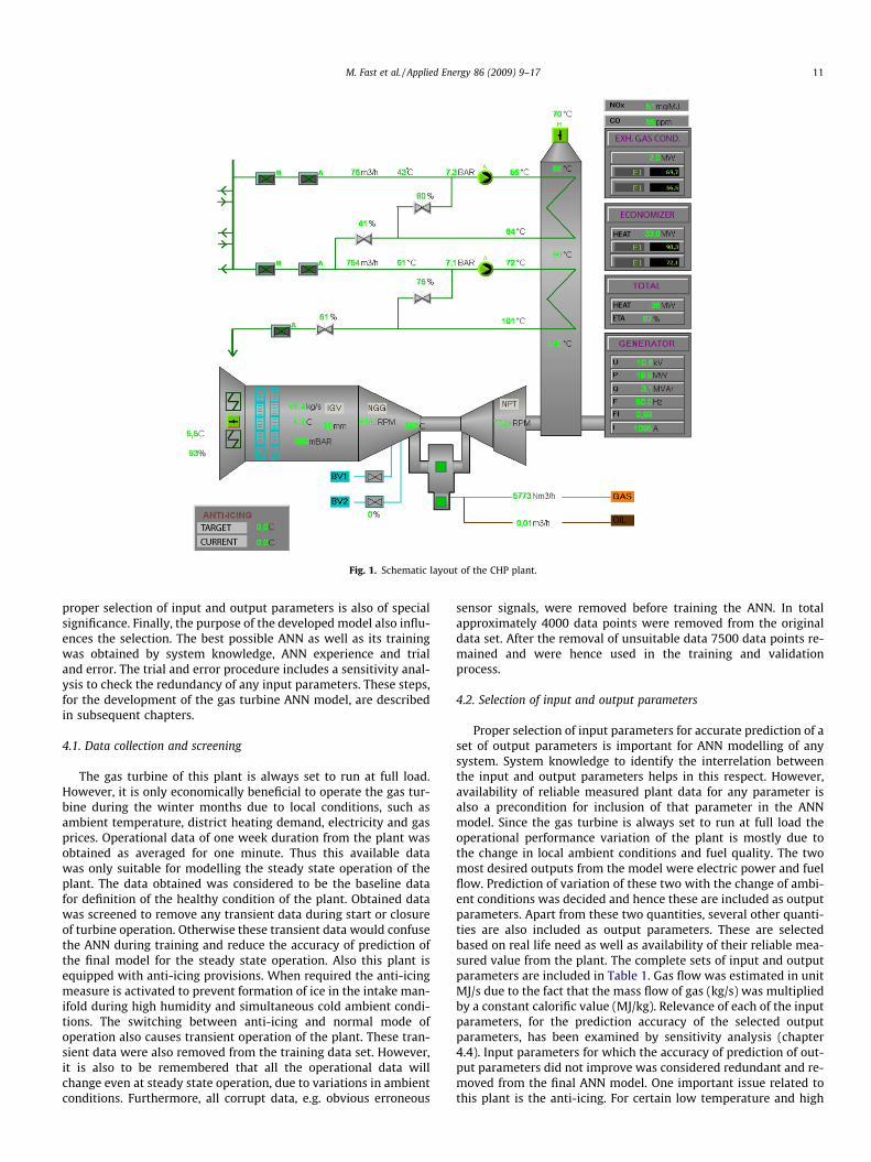
Fig. 1. Schematic layout of the CHP plant.

M. Fast et al. / Applied Energy 86 (2009) 9–17 11

proper selection of input and output parameters is also of specialsignificance. Finally, the purpose of the developed model also influ-ences the selection. The best possible ANN as well as its trainingwas obtained by system knowledge, ANN experience and trialand error. The trial and error procedure includes a sensitivity anal-ysis to check the redundancy of any input parameters. These steps,for the development of the gas turbine ANN model, are describedin subsequent chapters.

4.1. Data collection and screening

The gas turbine of this plant is always set to run at full load.However, it is only economically beneficial to operate the gas tur-bine during the winter months due to local conditions, such asambient temperature, district heating demand, electricity and gasprices. Operational data of one week duration from the plant wasobtained as averaged for one minute. Thus this available datawas only suitable for modelling the steady state operation of theplant. The data obtained was considered to be the baseline datafor definition of the healthy condition of the plant. Obtained datawas screened to remove any transient data during start or closureof turbine operation. Otherwise these transient data would confusethe ANN during training and reduce the accuracy of prediction ofthe final model for the steady state operation. Also this plant isequipped with anti-icing provisions. When required the anti-icingmeasure is activated to prevent formation of ice in the intake man-ifold during high humidity and simultaneous cold ambient condi-tions. The switching between anti-icing and normal mode ofoperation also causes transient operation of the plant. These tran-sient data were also removed from the training data set. However,it is also to be remembered that all the operational data willchange even at steady state operation, due to variations in ambientconditions. Furthermore, all corrupt data, e.g. obvious erroneous

sensor signals, were removed before training the ANN. In totalapproximately 4000 data points were removed from the originaldata set. After the removal of unsuitable data 7500 data points re-mained and were hence used in the training and validationprocess.

4.2. Selection of input and output parameters

Proper selection of input parameters for accurate prediction of aset of output parameters is important for ANN modelling of anysystem. System knowledge to identify the interrelation betweenthe input and output parameters helps in this respect. However,availability of reliable measured plant data for any parameter isalso a precondition for inclusion of that parameter in the ANNmodel. Since the gas turbine is always set to run at full load theoperational performance variation of the plant is mostly due tothe change in local ambient conditions and fuel quality. The twomost desired outputs from the model were electric power and fuelflow. Prediction of variation of these two with the change of ambi-ent conditions was decided and hence these are included as outputparameters. Apart from these two quantities, several other quanti-ties are also included as output parameters. These are selectedbased on real life need as well as availability of their reliable mea-sured value from the plant. The complete sets of input and outputparameters are included in Table 1. Gas flow was estimated in unitMJ/s due to the fact that the mass flow of gas (kg/s) was multipliedby a constant calorific value (MJ/kg). Relevance of each of the inputparameters, for the prediction accuracy of the selected outputparameters, has been examined by sensitivity analysis (chapter4.4). Input parameters for which the accuracy of prediction of out-put parameters did not improve was considered redundant and re-moved from the final ANN model. One important issue related tothis plant is the anti-icing. For certain low temperature and high

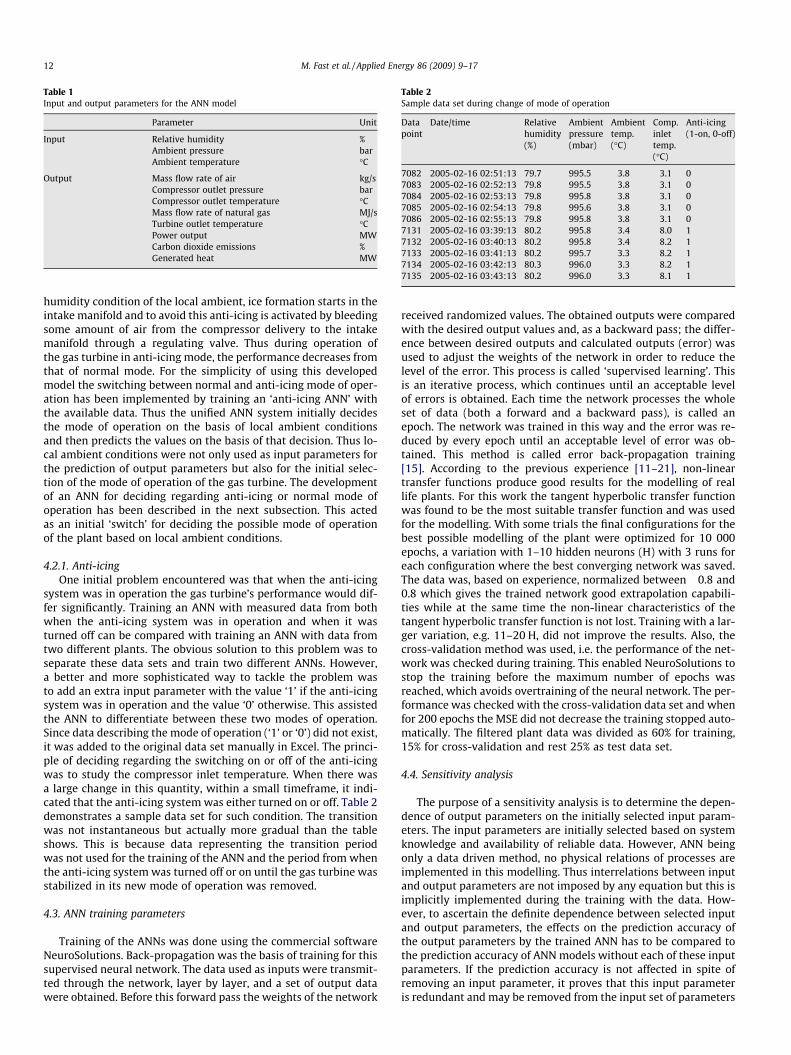
Table 1Input and output parameters for the ANN model

Parameter Unit

Input Relative humidity %Ambient pressure barAmbient temperature �C

Output Mass flow rate of air kg/sCompressor outlet pressure barCompressor outlet temperature �CMass flow rate of natural gas MJ/sTurbine outlet temperature �CPower output MWCarbon dioxide emissions %Generated heat MW

Table 2Sample data set during change of mode of operation

Datapoint

Date/time Relativehumidity(%)

Ambientpressure(mbar)

Ambienttemp.(�C)

Comp.inlettemp.(�C)

Anti-icing(1-on, 0-off)

7082 2005-02-16 02:51:13 79.7 995.5 �3.8 �3.1 07083 2005-02-16 02:52:13 79.8 995.5 �3.8 �3.1 07084 2005-02-16 02:53:13 79.8 995.8 �3.8 �3.1 07085 2005-02-16 02:54:13 79.8 995.6 �3.8 �3.1 07086 2005-02-16 02:55:13 79.8 995.8 �3.8 �3.1 07131 2005-02-16 03:39:13 80.2 995.8 �3.4 8.0 17132 2005-02-16 03:40:13 80.2 995.8 �3.4 8.2 17133 2005-02-16 03:41:13 80.2 995.7 �3.3 8.2 17134 2005-02-16 03:42:13 80.3 996.0 �3.3 8.2 17135 2005-02-16 03:43:13 80.2 996.0 �3.3 8.1 1

12 M. Fast et al. / Applied Energy 86 (2009) 9–17

humidity condition of the local ambient, ice formation starts in theintake manifold and to avoid this anti-icing is activated by bleedingsome amount of air from the compressor delivery to the intakemanifold through a regulating valve. Thus during operation ofthe gas turbine in anti-icing mode, the performance decreases fromthat of normal mode. For the simplicity of using this developedmodel the switching between normal and anti-icing mode of oper-ation has been implemented by training an ‘anti-icing ANN’ withthe available data. Thus the unified ANN system initially decidesthe mode of operation on the basis of local ambient conditionsand then predicts the values on the basis of that decision. Thus lo-cal ambient conditions were not only used as input parameters forthe prediction of output parameters but also for the initial selec-tion of the mode of operation of the gas turbine. The developmentof an ANN for deciding regarding anti-icing or normal mode ofoperation has been described in the next subsection. This actedas an initial ‘switch’ for deciding the possible mode of operationof the plant based on local ambient conditions.

4.2.1. Anti-icingOne initial problem encountered was that when the anti-icing

system was in operation the gas turbine’s performance would dif-fer significantly. Training an ANN with measured data from bothwhen the anti-icing system was in operation and when it wasturned off can be compared with training an ANN with data fromtwo different plants. The obvious solution to this problem was toseparate these data sets and train two different ANNs. However,a better and more sophisticated way to tackle the problem wasto add an extra input parameter with the value ‘1’ if the anti-icingsystem was in operation and the value ‘0’ otherwise. This assistedthe ANN to differentiate between these two modes of operation.Since data describing the mode of operation (‘1’ or ‘0’) did not exist,it was added to the original data set manually in Excel. The princi-ple of deciding regarding the switching on or off of the anti-icingwas to study the compressor inlet temperature. When there wasa large change in this quantity, within a small timeframe, it indi-cated that the anti-icing system was either turned on or off. Table 2demonstrates a sample data set for such condition. The transitionwas not instantaneous but actually more gradual than the tableshows. This is because data representing the transition periodwas not used for the training of the ANN and the period from whenthe anti-icing system was turned off or on until the gas turbine wasstabilized in its new mode of operation was removed.

4.3. ANN training parameters

Training of the ANNs was done using the commercial softwareNeuroSolutions. Back-propagation was the basis of training for thissupervised neural network. The data used as inputs were transmit-ted through the network, layer by layer, and a set of output datawere obtained. Before this forward pass the weights of the network

received randomized values. The obtained outputs were comparedwith the desired output values and, as a backward pass; the differ-ence between desired outputs and calculated outputs (error) wasused to adjust the weights of the network in order to reduce thelevel of the error. This process is called ‘supervised learning’. Thisis an iterative process, which continues until an acceptable levelof errors is obtained. Each time the network processes the wholeset of data (both a forward and a backward pass), is called anepoch. The network was trained in this way and the error was re-duced by every epoch until an acceptable level of error was ob-tained. This method is called error back-propagation training[15]. According to the previous experience [11–21], non-lineartransfer functions produce good results for the modelling of reallife plants. For this work the tangent hyperbolic transfer functionwas found to be the most suitable transfer function and was usedfor the modelling. With some trials the final configurations for thebest possible modelling of the plant were optimized for 10 000epochs, a variation with 1–10 hidden neurons (H) with 3 runs foreach configuration where the best converging network was saved.The data was, based on experience, normalized between �0.8 and0.8 which gives the trained network good extrapolation capabili-ties while at the same time the non-linear characteristics of thetangent hyperbolic transfer function is not lost. Training with a lar-ger variation, e.g. 11–20 H, did not improve the results. Also, thecross-validation method was used, i.e. the performance of the net-work was checked during training. This enabled NeuroSolutions tostop the training before the maximum number of epochs wasreached, which avoids overtraining of the neural network. The per-formance was checked with the cross-validation data set and whenfor 200 epochs the MSE did not decrease the training stopped auto-matically. The filtered plant data was divided as 60% for training,15% for cross-validation and rest 25% as test data set.

4.4. Sensitivity analysis

The purpose of a sensitivity analysis is to determine the depen-dence of output parameters on the initially selected input param-eters. The input parameters are initially selected based on systemknowledge and availability of reliable data. However, ANN beingonly a data driven method, no physical relations of processes areimplemented in this modelling. Thus interrelations between inputand output parameters are not imposed by any equation but this isimplicitly implemented during the training with the data. How-ever, to ascertain the definite dependence between selected inputand output parameters, the effects on the prediction accuracy ofthe output parameters by the trained ANN has to be compared tothe prediction accuracy of ANN models without each of these inputparameters. If the prediction accuracy is not affected in spite ofremoving an input parameter, it proves that this input parameteris redundant and may be removed from the input set of parameters

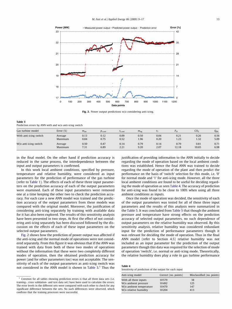
0

7

14

21

28

35

42

17

18

19

20

21

22

23

0 100 200 300 400 500 600 700 800 900 1000 1100 1200

Error [%]Power [MW]

Data points

Measured power output Predicted power output Prediction error

Fig. 2. Power output predictions w/o considering anti-icing.

Table 3Prediction errors by ANN with and w/o anti-icing switch

Gas turbine model Error (%) mair pc,out tc,out mng t7 Pel CO2 Qdh

With anti-icing switch Average 0.13 0.12 0.09 0.50 0.04 0.21 0.26 0.56Maximum 0.84 0.75 0.52 1.96 0.20 1.23 1.32 5.09

W/o anti-icing switch Average 0.50 0.47 0.14 0.79 0.14 0.79 0.81 0.71Maximum 7.31 6.89 2.21 9.20 2.07 12.18 10.65 6.98

Table 4Sensitivity of prediction of the output for each input

M. Fast et al. / Applied Energy 86 (2009) 9–17 13

in the final model. On the other hand if prediction accuracy isreduced in the same process, the interdependence between theinput and output parameters is confirmed.

In this work local ambient conditions, specified by pressure,temperature and relative humidity, were considered as inputparameters for the prediction of performance of the gas turbine(refer to Table 1). The effects of each of these three input parame-ters on the prediction accuracy of each of the output parameterswere examined. Each of these input parameters were removedone at a time keeping the other two to check the prediction accu-racy. For each case a new ANN model was trained and the predic-tion accuracy of the output parameters from these models wascompared with the original model. Moreover, the justification ofconsidering anti-icing separately by training with available datafor it has also been explored. The results of this sensitivity analysishave been presented in two steps. At first the effect of not consid-ering anti-icing separately has been discussed followed by the dis-cussion on the effects of each of these input parameters on theselected output parameters.

Fig. 2 shows how the prediction of power output was affected ifthe anti-icing and the normal mode of operations were not consid-ered separately. From this figure it was obvious that if the ANN wastrained with data from both of these two modes of operationswithout the information that these were two completely differentmodes of operation, then the obtained prediction accuracy forpower (and for other parameters too) was not acceptable. The sen-sitivity of each of the output parameters as anti-icing switch wasnot considered in the ANN model is shown in Table 3.1 Thus the

1 Common for all tables showing prediction errors is that all three data sets (i.e.training-, cross validation- and test data set) have been used to calculate the errors.The error levels in the different sets were compared with each other to check for anysignificant difference between the sets. No such differences were observed, whichconfirms that the training processes were successful.

justification of providing information to the ANN initially to decideregarding the mode of operation based on the local ambient condi-tions was established. Hence the final ANN was trained to decideregarding the mode of operation of the plant and then predict theperformance on the basis of ‘switch’ selection for this mode, i.e. ‘0’for normal mode and ‘1’ for anti-icing mode. However, all the threelocal ambient conditions are found to be useful for deciding regard-ing the mode of operation as seen Table 4. The accuracy of predictionfor anti-icing was found to be close to 100% when using all threeambient conditions as inputs.

Once the mode of operation was decided, the sensitivity of eachof the output parameters was tested for all of these three inputparameters and the results of this analysis were summarized inthe Table 5. It was concluded from Table 5 that though the ambientpressure and temperature have strong effects on the predictionaccuracy of selected output parameters, no such dependence ofoutput parameters on the relative humidity was observed. By thissensitivity analysis, relative humidity was considered redundantinput for the prediction of performance parameters though itwas relevant for deciding the mode of operation. Thus in the finalANN model (refer to Section 4.5) relative humidity was notincluded as an input parameter for the prediction of the outputparameters though this data was required for the selection of modeof operation ‘switch’, i.e. normal or anti-icing mode. Theoretically,the relative humidity does play a role in gas turbine performance

Anti-icing model Correct (no. points) Misclassified (no. points)

With all three inputs 10579 38W/o ambient pressure 10492 125W/o ambient temperature 10470 147W/o relative humidity 10204 413

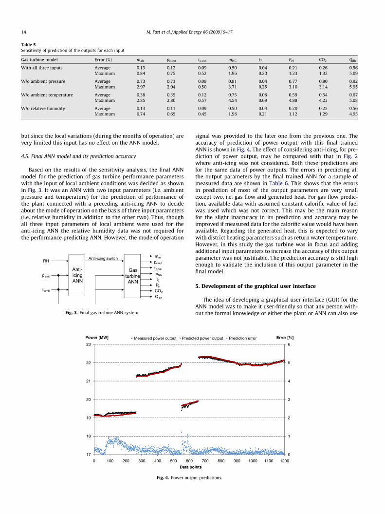
Table 5Sensitivity of prediction of the outputs for each input

Gas turbine model Error (%) mair pc,out tc,out mNG t7 Pel CO2 Qdh

With all three inputs Average 0.13 0.12 0.09 0.50 0.04 0.21 0.26 0.56Maximum 0.84 0.75 0.52 1.96 0.20 1.23 1.32 5.09

W/o ambient pressure Average 0.73 0.73 0.09 0.91 0.04 0.77 0.80 0.92Maximum 2.97 2.94 0.50 3.71 0.25 3.10 3.14 5.95

W/o ambient temperature Average 0.38 0.35 0.12 0.75 0.08 0.59 0.54 0.67Maximum 2.85 2.80 0.57 4.54 0.69 4.88 4.23 5.08

W/o relative humidity Average 0.13 0.11 0.09 0.50 0.04 0.20 0.25 0.56Maximum 0.74 0.65 0.45 1.98 0.21 1.12 1.29 4.95

14 M. Fast et al. / Applied Energy 86 (2009) 9–17

but since the local variations (during the months of operation) arevery limited this input has no effect on the ANN model.

4.5. Final ANN model and its prediction accuracy

Based on the results of the sensitivity analysis, the final ANNmodel for the prediction of gas turbine performance parameterswith the input of local ambient conditions was decided as shownin Fig. 3. It was an ANN with two input parameters (i.e. ambientpressure and temperature) for the prediction of performance ofthe plant connected with a preceding anti-icing ANN to decideabout the mode of operation on the basis of three input parameters(i.e. relative humidity in addition to the other two). Thus, thoughall three input parameters of local ambient were used for theanti-icing ANN the relative humidity data was not required forthe performance predicting ANN. However, the mode of operation

Anti-icingANN

RH

pamb

t amb

Anti-icing switch mair

pc,out

tc,out

mNG

t7

Pel

Q dh

GasturbineANN

CO2

Fig. 3. Final gas turbine ANN system.

17

18

19

20

21

22

23

0 100 200 300 400 500 600

Power [MW]

Data po

Measured power output Predict

Fig. 4. Power outp

signal was provided to the later one from the previous one. Theaccuracy of prediction of power output with this final trainedANN is shown in Fig. 4. The effect of considering anti-icing, for pre-diction of power output, may be compared with that in Fig. 2where anti-icing was not considered. Both these predictions arefor the same data of power outputs. The errors in predicting allthe output parameters by the final trained ANN for a sample ofmeasured data are shown in Table 6. This shows that the errorsin prediction of most of the output parameters are very smallexcept two, i.e. gas flow and generated heat. For gas flow predic-tion, available data with assumed constant calorific value of fuelwas used which was not correct. This may be the main reasonfor the slight inaccuracy in its prediction and accuracy may beimproved if measured data for the calorific value would have beenavailable. Regarding the generated heat, this is expected to varywith district heating parameters such as return water temperature.However, in this study the gas turbine was in focus and addingadditional input parameters to increase the accuracy of this outputparameter was not justifiable. The prediction accuracy is still highenough to validate the inclusion of this output parameter in thefinal model.

5. Development of the graphical user interface

The idea of developing a graphical user interface (GUI) for theANN model was to make it user-friendly so that any person with-out the formal knowledge of either the plant or ANN can also use

0

1

2

3

4

5

6

700 800 900 1000 1100 1200

Error [%]

ints

ed power output Prediction error

ut predictions.

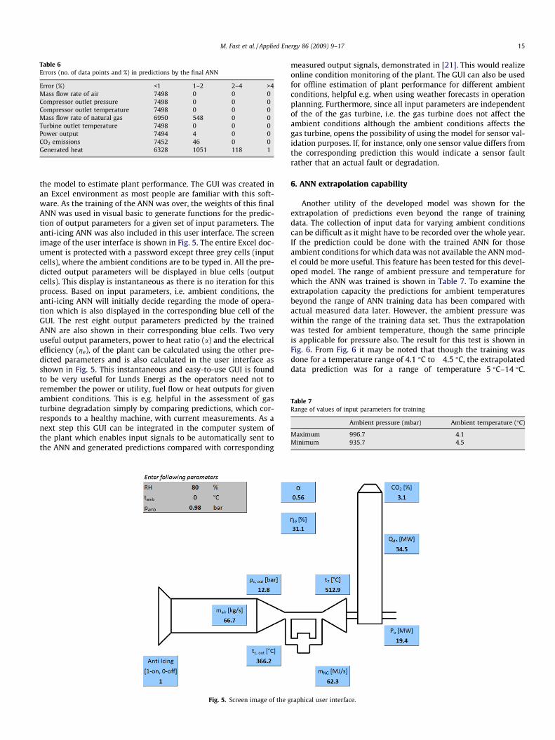
Table 6Errors (no. of data points and %) in predictions by the final ANN

Error (%) <1 1–2 2–4 >4Mass flow rate of air 7498 0 0 0Compressor outlet pressure 7498 0 0 0Compressor outlet temperature 7498 0 0 0Mass flow rate of natural gas 6950 548 0 0Turbine outlet temperature 7498 0 0 0Power output 7494 4 0 0CO2 emissions 7452 46 0 0Generated heat 6328 1051 118 1

Table 7Range of values of input parameters for training

Ambient pressure (mbar) Ambient temperature (�C)

Maximum 996.7 4.1Minimum 935.7 �4.5

M. Fast et al. / Applied Energy 86 (2009) 9–17 15

the model to estimate plant performance. The GUI was created inan Excel environment as most people are familiar with this soft-ware. As the training of the ANN was over, the weights of this finalANN was used in visual basic to generate functions for the predic-tion of output parameters for a given set of input parameters. Theanti-icing ANN was also included in this user interface. The screenimage of the user interface is shown in Fig. 5. The entire Excel doc-ument is protected with a password except three grey cells (inputcells), where the ambient conditions are to be typed in. All the pre-dicted output parameters will be displayed in blue cells (outputcells). This display is instantaneous as there is no iteration for thisprocess. Based on input parameters, i.e. ambient conditions, theanti-icing ANN will initially decide regarding the mode of opera-tion which is also displayed in the corresponding blue cell of theGUI. The rest eight output parameters predicted by the trainedANN are also shown in their corresponding blue cells. Two veryuseful output parameters, power to heat ratio (a) and the electricalefficiency (ge), of the plant can be calculated using the other pre-dicted parameters and is also calculated in the user interface asshown in Fig. 5. This instantaneous and easy-to-use GUI is foundto be very useful for Lunds Energi as the operators need not toremember the power or utility, fuel flow or heat outputs for givenambient conditions. This is e.g. helpful in the assessment of gasturbine degradation simply by comparing predictions, which cor-responds to a healthy machine, with current measurements. As anext step this GUI can be integrated in the computer system ofthe plant which enables input signals to be automatically sent tothe ANN and generated predictions compared with corresponding

Fig. 5. Screen image of the g

measured output signals, demonstrated in [21]. This would realizeonline condition monitoring of the plant. The GUI can also be usedfor offline estimation of plant performance for different ambientconditions, helpful e.g. when using weather forecasts in operationplanning. Furthermore, since all input parameters are independentof the of the gas turbine, i.e. the gas turbine does not affect theambient conditions although the ambient conditions affects thegas turbine, opens the possibility of using the model for sensor val-idation purposes. If, for instance, only one sensor value differs fromthe corresponding prediction this would indicate a sensor faultrather that an actual fault or degradation.

6. ANN extrapolation capability

Another utility of the developed model was shown for theextrapolation of predictions even beyond the range of trainingdata. The collection of input data for varying ambient conditionscan be difficult as it might have to be recorded over the whole year.If the prediction could be done with the trained ANN for thoseambient conditions for which data was not available the ANN mod-el could be more useful. This feature has been tested for this devel-oped model. The range of ambient pressure and temperature forwhich the ANN was trained is shown in Table 7. To examine theextrapolation capacity the predictions for ambient temperaturesbeyond the range of ANN training data has been compared withactual measured data later. However, the ambient pressure waswithin the range of the training data set. Thus the extrapolationwas tested for ambient temperature, though the same principleis applicable for pressure also. The result for this test is shown inFig. 6. From Fig. 6 it may be noted that though the training wasdone for a temperature range of 4.1 �C to �4.5 �C, the extrapolateddata prediction was for a range of temperature 5 �C–14 �C.

raphical user interface.

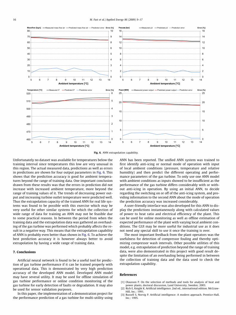
0

1

3

4

5

6

8

9

10

0

10

20

30

40

50

60

70

80

5 6 7 8 9 10 11 12 13 14 5 6 7 8 9 10 11 12 13 14

5 6 7 8 9 10 11 12 13 145 6 7 8 9 10 11 12 13 14

Error [%]Massflow [kg/s]

Ambient temperature [°C]

Measured mass flow air Predicted mass flow air Prediction error

0

2

4

6

8

10

12

14

16

0

2

4

6

8

10

12

14

16Error [%]Pressure [bar]

Ambient temperature [°C]

Measured p3 Predicted p3 Prediction error

0

1

2

3

4

5

6

460

470

480

490

500

510

520Error [%]Temperature [°C]

Ambient temperature [°C]

Measured t7 Predicted t7 Prediction error

0

5

10

15

20

25

0

5

10

15

20

25Error [%]Power [MW]

Ambient temperature [°C]

Measured power output Predicted power output Prediction error

Fig. 6. ANN extrapolation capability.

16 M. Fast et al. / Applied Energy 86 (2009) 9–17

Unfortunately no dataset was available for temperatures below thetraining interval since temperatures this low are very unusual inthis region. The actual measured data, predictions as well as errorsin predictions are shown for four output parameters in Fig. 6. Thisshows that the prediction accuracy is good for ambient tempera-tures beyond the range of training data. One important conclusiondrawn from these results was that the errors in prediction did notincrease with increased ambient temperature, more beyond therange of training values of it. The trends of decreasing power out-put and increasing turbine outlet temperature were predicted well.Thus the extrapolation capacity of the trained ANN for real life sys-tems was found to be possible with this exercise which may bevery useful for other similar systems for which the collection ofwide range of data for training an ANN may not be feasible dueto some practical reasons. In between the period from when thetraining data and the extrapolation data was gathered an overhaul-ing of the gas turbine was performed which probably affects the re-sult in a negative way. This means that the extrapolation capabilityof ANN is probably even better than shown in Fig. 6. To achieve thebest prediction accuracy it is however always better to avoidextrapolation by having a wide range of training data.

7. Conclusions

Artificial neural network is found to be a useful tool for predic-tion of gas turbine performance if it can be trained properly withoperational data. This is demonstrated by very high predictionaccuracy of the developed ANN model. Developed ANN modelmay have several utility. It may be used for offline simulation ofgas turbine performance or online condition monitoring of thegas turbine for early detection of faults or degradation. It may alsobe used for sensor validation purposes.

In this paper, the implementation of a demonstration project forthe performance prediction of a gas turbine for multi-utility using

ANN has been reported. The unified ANN system was trained tofirst identify anti-icing or normal mode of operation with inputof local ambient conditions (pressure, temperature and relativehumidity) and then predict the different operating and perfor-mance parameters of the gas turbine. To only use one ANN modelwith ambient conditions as inputs showed to be insufficient as theperformance of the gas turbine differs considerably with or with-out anti-icing in operation. By using an initial ANN, to decideregarding the switching on or off of the anti-icing system, and pro-viding information to the second ANN about the mode of operationthe prediction accuracy was increased considerably.

A user-friendly interface was also developed for this ANN to dis-play the predictions instantaneously along with calculated valuesof power to heat ratio and electrical efficiency of the plant. Thiscan be used for online monitoring as well as offline estimation ofexpected performance of the plant with varying local ambient con-ditions. The GUI may be more useful for industrial use as it doesnot need any special skill to use it once the training is over.

The most important feedback from the plant operators was theusefulness for detection of compressor fouling and thereby opti-mizing compressor wash intervals. Other possible utilities of thismodel, e.g. extrapolation of prediction beyond the range of trainingdata, were also demonstrated in this project with good result de-spite the limitation of an overhauling being performed in betweenthe collection of training data and the data used to check theextrapolation capability.

References

[1] Olausson P. On the selection of methods and tools for analysis of heat andpower plants, doctoral discussion, Lund University, Sweden; 2003.

[2] Rich E, Knight K. Artificial intelligence. 2nd ed., international edition. McGraw-Hill, Inc.; 1991.

[3] Russell S, Norvig P. Artificial intelligence: A modern approach. Prentice-Hall,Inc.; 1995.

M. Fast et al. / Applied Energy 86 (2009) 9–17 17

[4] Haykin S. Neural networks, a comprehensive foundation. 2nd ed. New Jersey,USA: Prentice-Hall Inc.; 1999.

[5] DePold H, Douglas Gass F. The application of expert systems and neuralnetworks to gas turbine prognostics and diagnostics. In: ASME internationalgas turbine & aeroengine congress & exhibition, Paper no. 98-GT-101; 1998.

[6] Embrechts M, Schweizerhof A, Bushman M, Sabatella M. Neural networkmodelling of turbofan parameters. In: ASME turbo expo, Paper no. 2000-GT-0036; 2000.

[7] Bettocchi R, Spina P, Torella G. Gas turbine health indices determination usingneural networks. In: ASME turbo expo, Paper no. GT-2002-30276; 2002.

[8] Perryman R, Perrot S. Condition monitoring and predictive analysis ofcombined heat and power systems. UK: University of Greenwich; 1994.

[9] Boccaletti C, Cerri G, Seyedan B. A neural network simulator of a gas turbinewith a waste heat recovery section. J Eng Gas Turbine Power 2001;123:371–6.

[10] Ferrettl G, Piroddi L. Estimation of NOX emissions in thermal power plantsusing neural network. J Eng Gas Turbine Power 2001;123:465–71.

[11] Mesbahi E, Assadi M, Torisson T, Lindquist T. A unique correction technique forevaporative gas turbine (EvGT) parameters, ASME turbo expo; 2001.

[12] Mesbahi E, Assadi M, Torisson T. An online and remote sensor validation andcondition monitoring system for power plants, CIMAC; 2001.

[13] Mesbahi E, Genrup M, Assadi M. Fault prediction/diagnosis and sensorvalidation technique for a steam power plant. J Marine Eng Technol A2005;7:33–40.

[14] Arriagada J, Costantini M, Olausson P, Assadi M, Torisson T. Artificial neuralnetwork model for a biomass-fuelled boiler. In: ASME turbo expo, Paper no.GT2003-38070; 2003.

[15] Arriagada J. Introduction of intelligent tools for gas turbine based, small-scalecogeneration, Licentiate thesis, Lund University, Sweden; 2001.

[16] Arriagada J. On the analysis and fault diagnosis tools for small scale heat andpower plants, doctoral discussion, Lund University, Sweden; 2003.

[17] Arriagada J, Genrup M, Loberg A, Assadi M. Fault diagnosis system for anindustrial gas turbine by means of neural networks, IGTC; 2003.

[18] Assadi M, Mesbahi E, Torisson T, Lindquist T, Arriagada J, Olausson P. A Novelcorrection technique for simple gas turbine parameters. In: ASME turbo expo;2001.

[19] Fast M. Artificial neural networks for gas turbine modelling and sensorvalidation, Master thesis, Lund University, Sweden; 2005.

[20] De S, Kaiadi M, Fast M, Assadi M. Development of an artificial neural networkmodel for the steam process of a coal biomass co-fired combined heat andpower (CHP) plant in Sweden. Energy 2007;32(11):2099–109.

[21] Fast M, Assadi M, Smrekar J. Application of artificial neural network to thecondition monitoring and diagnosis of a CHP plant, ECOS; accepted forpublication.

[22] Cybenko G. Approximation by superpositions of a sigmoidal function. MathControl Signals Syst 1989;2:303–14.

[23] Siemens webpage. www.powergeneration.siemens.com; March 2008.[24] Lunds Energi webpage. www.lundsenergi.se; March 2008.

Application of artificial neural network to the condition monitoring and

diagnosis of a combined heat and power plant Fast M, Palmé T.

Journal of Energy, Vol. 35, Issue 2, pp. 1114-1120, February 2010

Paper II

Author's personal copy

Application of artificial neural networks to the condition monitoring anddiagnosis of a combined heat and power plant

M. Fast a,*, T. Palme b

a Division of Thermal Power Engineering, Department of Energy Sciences, Lund University, P.O. Box 118, S-221 00 Lund, Swedenb Department of Mechanical and Structural Engineering and Materials Science, University of Stavanger, N-4036 Stavanger, Norway

a r t i c l e i n f o

Article history:Received 30 October 2008Received in revised form29 May 2009Accepted 12 June 2009Available online 16 July 2009

Keywords:Power plantArtificial neural networkMonitoringDiagnosis

a b s t r a c t

The objective of this study has been to create an online system for condition monitoring and diagnosis ofa combined heat and power plant in Sweden. The system in question consisted of artificial neuralnetwork models, representing each main component of the combined heat and power plant, connectedto a graphical user interface. The artificial neural network models were integrated on a power generationinformation manager server in the computer system of the combined heat and power plant, and thegraphical user interface was made available on workstations connected to this server.

The plant comprised a Siemens SGT800 gas turbine with a heat recovery steam generator as well asa bio-fueled boiler and its steam cycle. Steam from the heat recovery steam generator and the bio-fueledboiler expanded together in a common steam turbine, producing both electricity and heat. The artificialneural network models were trained with operational data from the components of the combined heatand power plant.

Accurate predictions from the ANN (Artificial neural network) models in combination with an unde-manding integration in the power plant’s computer system were some of the main conclusions from thisstudy.

� 2009 Elsevier Ltd. All rights reserved.

1. Introduction

The main interest of the present research includes an increasedavailability, a reduced maintenance cost as well as a more efficientmaintenance, i.e., condition-based maintenance. By linking histor-ical operational data to the analysis of plant condition, an optimi-zation of maintenance and performance of a plant becomespossible. Deviations from an expected data pattern could indicatefor instance a faulty component or degradation, whereuponwarnings and/or alarms can be generated.

The plant studied is a hybrid combined heat and power (CHP)plant consisting of a gas turbine with its heat recovery steamgenerator and a biomass fueled boiler with its steam cycle. Artificialneural network (ANN) is the data modeling tool used for this studyand operational data the basis for training the networks.

Several authors have reported on a variety of applications, suchas monitoring, diagnosis, optimization, fault diagnosis etc., bymeans of data driven modeling. In [1] ANN is employed for theoptimization of load allocations and in [2] a fault diagnosis neuralnetwork is trained with operational data from a nuclear power

plant. Other examples include [3,4] where ANN is used for diag-nosis of a turbofan engine and fault diagnosis in a power plant.Researchers at the Division of Thermal Power Engineering at LundUniversity have carried out several investigations – References [5–8] representing some of them – in this field and ANN has proven tobe a good candidate for the modeling of non-linear energy systems.

The CHP plant components were simulated with ANN and themodels were integrated on a power generation informationmanager (PGIM) server in the computer system of the CHP plant.The PGIM server continuously receives signals from the plant andalso stores the signals for up to seven years. The ANN models are fedwith measured signals in real time to provide predictions of theexpected plant performance, and these predictions are presentedthrough a graphical user interface (GUI) and are also stored on theserver in the event that the plant’s performance history needs to beevaluated. Each time new predictions are calculated, a comparisonbetween these and the corresponding measured signals is made,whereupon warnings and/or alarms are generated for possibleanomalies. The warning and alarm limits can be individually set forall output parameters, according to, for example, operator demandsor ANN and sensor accuracy. If several warnings and/or alarmsoccur it could be an indication of degradation or component mal-function. In the case of a single warning or alarm, a faulty sensormay be the cause. Furthermore, production costs and income are

* Corresponding author. Tel.: þ46462229231; fax: þ46462224717.E-mail address: magnus.fast@energy.lth.se (M. Fast).

Contents lists available at ScienceDirect

Energy

journal homepage: www.elsevier .com/locate/energy

0360-5442/$ – see front matter � 2009 Elsevier Ltd. All rights reserved.doi:10.1016/j.energy.2009.06.005

Energy 35 (2010) 1114–1120

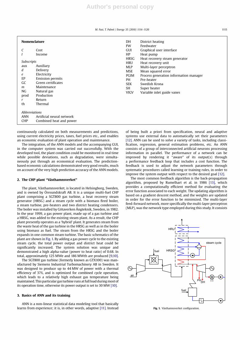
Author's personal copy

continuously calculated on both measurements and predictions,using current electricity prices, taxes, fuel prices etc., and enablesan economic evaluation of plant operation and maintenance.

The integration, of the ANN models and the accompanying GUI,in the computer system was carried out successfully. With thedeveloped tool, the plant condition could be monitored in real timewhile possible deviations, such as degradation, were simulta-neously put through an economical evaluation. The prediction-based economic calculations demonstrated very good results, muchon account of the very high prediction accuracy of the ANN models.

2. The CHP plant ‘‘Vasthamnsverket’’

The plant, Vasthamnsverket, is located in Helsingborg, Sweden,and is owned by Oresundskraft AB. It is a unique multi-fuel CHPplant comprising a SGT800 gas turbine, a heat recovery steamgenerator (HRSG) and a steam cycle with a biomass fired boiler,a steam turbine, pre-heaters and two district heating condensers.The boiler was installed by Gotaverken Ångteknik, Sweden, in 1982.In the year 1999, a gas power plant, made up of a gas turbine anda HRSG, was added to the existing steam plant. As a result, the CHPplant presently operates as a ‘hybrid’ plant. It generates steam fromthe waste heat of the gas turbine in the HRSG as well as in the boilerusing biomass as fuel. The steam from the HRSG and the boilerexpands in one common steam turbine. The basic schematics of theplant are shown in Fig. 1. By adding a gas power cycle to the existingsteam cycle, the total power output and district heat could besignificantly increased. The system solution was unique anddemonstrated a high alpha-value (power to heat ratio) of 0.68. Intotal, approximately 125 MWe and 186 MWth are produced [9,10].

The SGT800 gas turbine (formerly known as GTX100) was man-ufactured by Siemens Industrial Turbomachinery AB in Sweden. Itwas designed to produce up to 44 MW of power with a thermalefficiency of 37%, and is optimized for combined cycle operation,which leads to a relatively high exhaust gas temperature beingmaintained. This particular gas turbine runs at full load during most ofits operation time, otherwise its power output is set to 30 MW [10].

3. Basics of ANN and its training

ANN is a non-linear statistical data modeling tool that basicallylearns from experience; it is, in other words, adaptive [11]. Instead

of being built a priori from specification, neural and adaptivesystems use external data to automatically set their parameters[12]. ANN can be used to solve a variety of tasks, including classi-fication, regression, general estimation problems, etc. An ANNconsists of a group of interconnected artificial neurons processinginformation in parallel. The performance of a network can beimproved by rendering it ‘‘aware’’ of its output(s) througha performance feedback loop that includes a cost function. Thefeedback is used to adjust the network parameters throughsystematic procedures called learning or training rules, in order toimprove the system output with respect to the desired goal [12].

The most common feedback algorithm is the back-propagationalgorithm, proposed by Rumelhart et al. in 1986 [13], whichprovides a computationally efficient method for evaluating theerror function associated to each weight. The updating algorithm isbased on a gradient descent method, and the weights are updatedin order for the error function to be minimized. The multi-layerfeed-forward network, more specifically the multi-layer perceptron(MLP), was the network type employed during this study. It consists

fuel

air

HRSG

steam cycle

HRU

fuel

PHDH

Fig. 1. Vasthamnsverket configuration.

Nomenclature

C CostI Income

Subscriptsaux Auxiliaryd Deliverye ElectricityEP Emission permitsGC Green certificatesm MaintenanceNG Natural gasprod Productionr Returnth Thermal

AbbreviationsANN Artificial neural networkCHP Combined heat and power

DH District heatingFW FeedwaterGUI Graphical user interfaceHP Heat pumpHRSG Heat recovery steam generatorHRU Heat recovery unitMLP Multi-layer perceptronMSE Mean squared errorPGIM Process generation information managerPH Pre-heaterSEK Swedish KronaSH Super heaterVIGV Variable inlet guide vanes

M. Fast, T. Palme / Energy 35 (2010) 1114–1120 1115

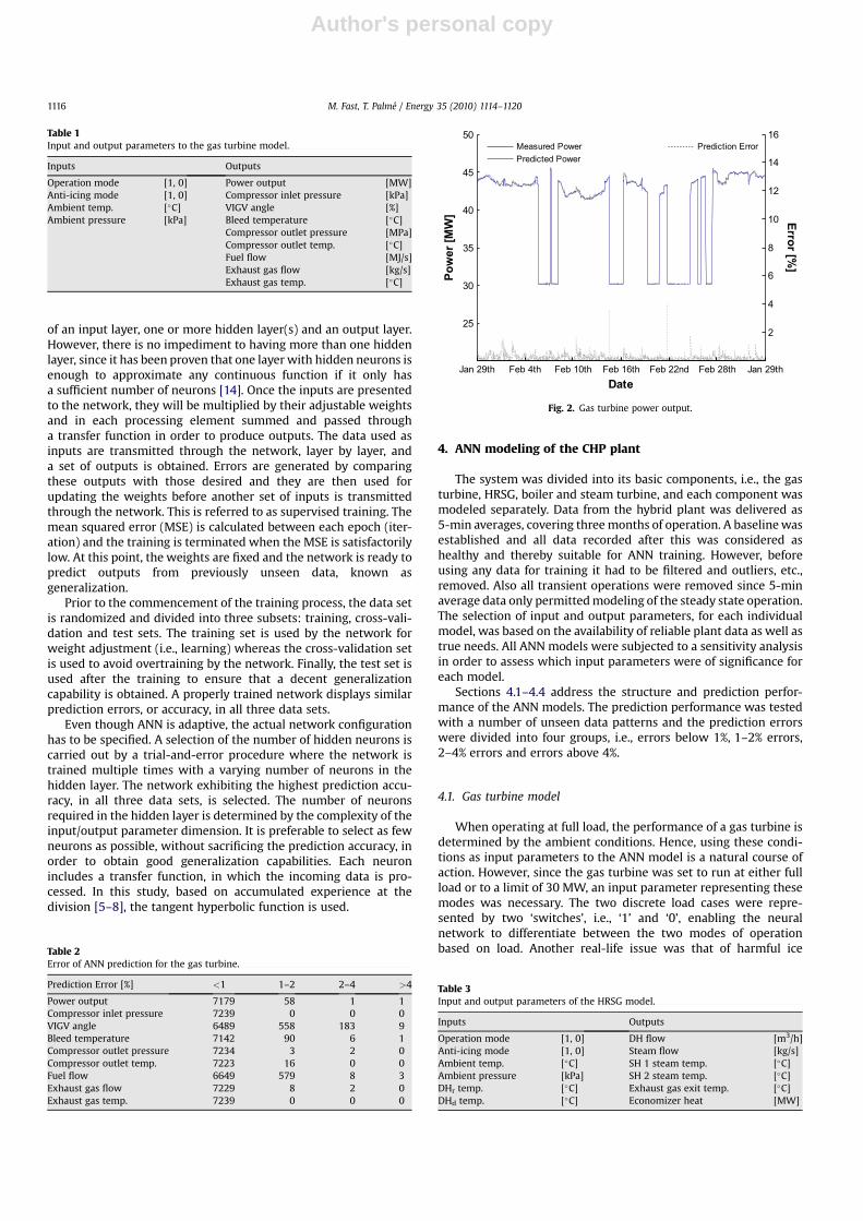
Author's personal copy

of an input layer, one or more hidden layer(s) and an output layer.However, there is no impediment to having more than one hiddenlayer, since it has been proven that one layer with hidden neurons isenough to approximate any continuous function if it only hasa sufficient number of neurons [14]. Once the inputs are presentedto the network, they will be multiplied by their adjustable weightsand in each processing element summed and passed througha transfer function in order to produce outputs. The data used asinputs are transmitted through the network, layer by layer, anda set of outputs is obtained. Errors are generated by comparingthese outputs with those desired and they are then used forupdating the weights before another set of inputs is transmittedthrough the network. This is referred to as supervised training. Themean squared error (MSE) is calculated between each epoch (iter-ation) and the training is terminated when the MSE is satisfactorilylow. At this point, the weights are fixed and the network is ready topredict outputs from previously unseen data, known asgeneralization.

Prior to the commencement of the training process, the data setis randomized and divided into three subsets: training, cross-vali-dation and test sets. The training set is used by the network forweight adjustment (i.e., learning) whereas the cross-validation setis used to avoid overtraining by the network. Finally, the test set isused after the training to ensure that a decent generalizationcapability is obtained. A properly trained network displays similarprediction errors, or accuracy, in all three data sets.

Even though ANN is adaptive, the actual network configurationhas to be specified. A selection of the number of hidden neurons iscarried out by a trial-and-error procedure where the network istrained multiple times with a varying number of neurons in thehidden layer. The network exhibiting the highest prediction accu-racy, in all three data sets, is selected. The number of neuronsrequired in the hidden layer is determined by the complexity of theinput/output parameter dimension. It is preferable to select as fewneurons as possible, without sacrificing the prediction accuracy, inorder to obtain good generalization capabilities. Each neuronincludes a transfer function, in which the incoming data is pro-cessed. In this study, based on accumulated experience at thedivision [5–8], the tangent hyperbolic function is used.

4. ANN modeling of the CHP plant

The system was divided into its basic components, i.e., the gasturbine, HRSG, boiler and steam turbine, and each component wasmodeled separately. Data from the hybrid plant was delivered as5-min averages, covering three months of operation. A baseline wasestablished and all data recorded after this was considered ashealthy and thereby suitable for ANN training. However, beforeusing any data for training it had to be filtered and outliers, etc.,removed. Also all transient operations were removed since 5-minaverage data only permitted modeling of the steady state operation.The selection of input and output parameters, for each individualmodel, was based on the availability of reliable plant data as well astrue needs. All ANN models were subjected to a sensitivity analysisin order to assess which input parameters were of significance foreach model.

Sections 4.1–4.4 address the structure and prediction perfor-mance of the ANN models. The prediction performance was testedwith a number of unseen data patterns and the prediction errorswere divided into four groups, i.e., errors below 1%, 1–2% errors,2–4% errors and errors above 4%.

4.1. Gas turbine model

When operating at full load, the performance of a gas turbine isdetermined by the ambient conditions. Hence, using these condi-tions as input parameters to the ANN model is a natural course ofaction. However, since the gas turbine was set to run at either fullload or to a limit of 30 MW, an input parameter representing thesemodes was necessary. The two discrete load cases were repre-sented by two ‘switches’, i.e., ‘1’ and ‘0’, enabling the neuralnetwork to differentiate between the two modes of operationbased on load. Another real-life issue was that of harmful ice

Table 1Input and output parameters to the gas turbine model.

Inputs Outputs

Operation mode [1, 0] Power output [MW]Anti-icing mode [1, 0] Compressor inlet pressure [kPa]Ambient temp. [�C] VIGV angle [%]Ambient pressure [kPa] Bleed temperature [�C]

Compressor outlet pressure [MPa]Compressor outlet temp. [�C]Fuel flow [MJ/s]Exhaust gas flow [kg/s]Exhaust gas temp. [�C]

Table 2Error of ANN prediction for the gas turbine.

Prediction Error [%] <1 1–2 2–4 >4

Power output 7179 58 1 1Compressor inlet pressure 7239 0 0 0VIGV angle 6489 558 183 9Bleed temperature 7142 90 6 1Compressor outlet pressure 7234 3 2 0Compressor outlet temp. 7223 16 0 0Fuel flow 6649 579 8 3Exhaust gas flow 7229 8 2 0Exhaust gas temp. 7239 0 0 0

25

30

35

40

45

50

Po

wer [M

W]

Measured PowerPredicted Power

Jan 29th Feb 4th Feb 10th Feb 16th Feb 22nd Feb 28th Jan 29th

2

4

6

8

10

12

14

16

Date

Erro

r [%

]

Prediction Error

Fig. 2. Gas turbine power output.

Table 3Input and output parameters of the HRSG model.

Inputs Outputs

Operation mode [1, 0] DH flow [m3/h]Anti-icing mode [1, 0] Steam flow [kg/s]Ambient temp. [�C] SH 1 steam temp. [�C]Ambient pressure [kPa] SH 2 steam temp. [�C]DHr temp. [�C] Exhaust gas exit temp. [�C]DHd temp. [�C] Economizer heat [MW]

M. Fast, T. Palme / Energy 35 (2010) 1114–11201116

Author's personal copy

formation in the intake manifold during local ambient conditionsthat were simultaneously cold and humid. To avoid this, an anti-icing system was utilized to preheat the air before the compressor.The anti-icing operation also constituted a discrete mode and wasrepresented by another set of ‘1’ and ‘0’ switches in the ANN model.A complete list of input and output parameters for this ANN ispresented in Table 1, and the ANN prediction accuracy is given inTable 2. Fig. 2 shows a comparison between measured and pre-dicted power together with the prediction error. Generally verygood prediction accuracy is attained with the gas turbine modeland most errors are below 1%. The VIGV (variable inlet guide vane)angle and the fuel flow are exhibiting somewhat elevated errorlevels in their prediction. The reason for the slightly higher errors ingas flow predictions can be referred to the fact that no consider-ation to variations in the calorific value of the fuel is taken. Also,during the collection of the data the control of the VIGVs wasexperiencing small fluctuations which are the reason behind thehigher prediction errors for this parameter.

4.2. HRSG model

The input parameters for the HRSG ANN were very similar to theones for the gas turbine ANN due to the fact that the gas turbinegoverned the performance of the HRSG. The difference wasconstituted by the fact that the HRSG was also affected by thedistrict heating circuit and the feedwater properties. A complete listof input and output parameters for the HRSG model can be seen inTable 3 and the prediction accuracy of the model is provided inTable 4. The temperature predictions are very good whereas flowand heat predictions have a lower accuracy. This difference is mostlikely the cause of flows being generally harder to measure withgood accuracy and the fact that sensors located on the districtheating circuit are not prioritized as high and thereby not calibratedregularly. All predictions are, however, sufficiently accurate.

4.3. Boiler model

Only two input parameters, i.e., the temperature and pressure ofthe feedwater, were required for the ANN boiler model in order toobtain predictions of the steam properties and the mass flow rate ofpellets. The in- and output parameters of the boiler model are listedin Table 5 and the error distributions for the predictions are pre-sented in Table 6.

4.4. Steam turbine model

The prediction of the power output and the produced heat in thedistrict heating condensers requires a number of input parameters.

The most obvious of these are the steam properties, both from theHRSG and the boiler, along with return and delivery temperaturesof the district heating. The heat generated in the boiler economizerand the heat pump are added as inputs since they are located on thesame district heating circuit as the condensers and thereby alsoaffect the system. Table 7 shows the model structure while Table 8and Fig. 3 illustrate the prediction performance of the model. Thepower output and the feedwater temperature are predicted verywell while the condenser heat exhibits larger prediction errors. Thecondenser heat is on the other hand calculated from several othermeasured parameters and this behavior is, therefore, expected.

5. Economic calculations

The idea behind the economics part is to always have two valuesof the production cost, i.e., actual and ‘‘predicted’’ values, thusallowing for instance an economical evaluation of the plantdegradation. This is possible since the ANN models always predictthe performance of a healthy plant and economic calculationsbased on these predictions will indicate what the production costshould be. Economic factors that are taken into account include fuelprices and taxes on fuels and energy production, etc. The produc-tion cost is divided between the two production types, i.e., gasturbine/natural gas and solid fuel boiler/pellets. Since these areclosely connected through the hybrid configuration, specialconsideration is needed when calculating the production cost.

Sections 5.1–5.3 briefly describe three types of control mecha-nisms applied for the energy sector in Sweden. Furthermore,Sections 5.4 and 5.5 explain the basics for calculating the produc-tion cost for the two production types.

5.1. Carbon dioxide tax

In order to reduce CO2 emissions, all fossil fuels, such as coal, oiland natural gas, are subject to a CO2 tax. However, electricityproduction is exempt of the tax and heat produced in combinedheat and power plants is only subject to 21% of it. Pure heatproduction, on the other hand, is subject to full, 100%, CO2 tax.Various fuels generate different amount of CO2 for which reason theCO2 tax varies depending on the fuel type [15].

5.2. Emission trading

The emission trading is a means of reducing the emission ofgreenhouse gases into the atmosphere, in accordance with the

Table 4Error of ANN prediction for the HRSG.

Prediction Error [%] <1 1–2 2–4 >4

DH flow 3387 2225 1188 165Steam flow 5757 1019 165 24SH 1 steam temp. 6949 16 0 0SH 2 steam temp. 6965 0 0 0Exhaust gas exit temp. 6481 464 17 3Economizer heat 4729 1711 453 72

Table 5Input and output parameters of the boiler model.

Inputs Outputs

FW temp. [�C] Steam flow [kg/s]FW pressure [MPa] Steam temperature [�C]

Pellets flow [kg/s]

Table 6Error of ANN prediction for the boiler.

Prediction Error [%] <1 1–2 2–4 >4

Steam flow 2628 229 25 18Steam temperature 2332 517 51 0Pellets flow 2462 400 30 8

Table 7Input and output parameters of the steam turbine model.

Inputs Outputs

Steam flow HRSG [kg/s] Power output [MW]Steam flow boiler [kg/s] FW temp. [�C]Steam temp. boiler [�C] Condenser heat [MW]DHr temp. [�C]DHd temp. [�C]HP heat [MW]Economizer heat boiler [MW]

M. Fast, T. Palme / Energy 35 (2010) 1114–1120 1117

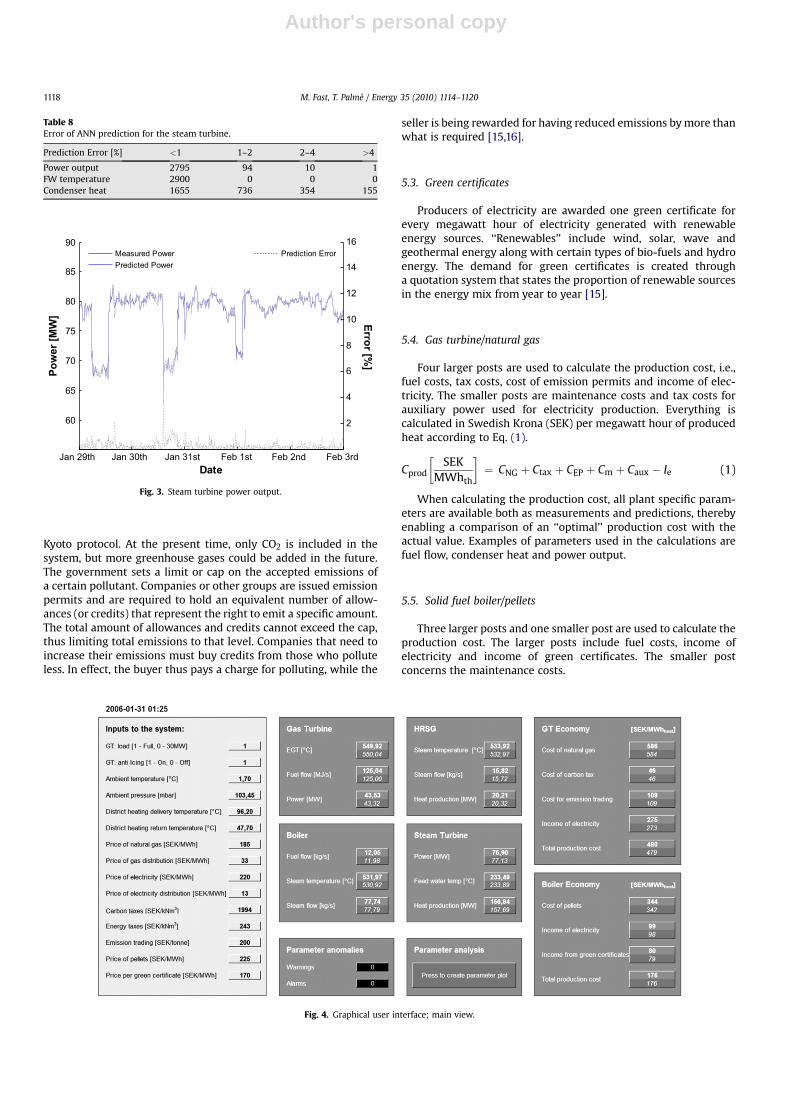
Author's personal copy

Kyoto protocol. At the present time, only CO2 is included in thesystem, but more greenhouse gases could be added in the future.The government sets a limit or cap on the accepted emissions ofa certain pollutant. Companies or other groups are issued emissionpermits and are required to hold an equivalent number of allow-ances (or credits) that represent the right to emit a specific amount.The total amount of allowances and credits cannot exceed the cap,thus limiting total emissions to that level. Companies that need toincrease their emissions must buy credits from those who polluteless. In effect, the buyer thus pays a charge for polluting, while the

seller is being rewarded for having reduced emissions by more thanwhat is required [15,16].

5.3. Green certificates

Producers of electricity are awarded one green certificate forevery megawatt hour of electricity generated with renewableenergy sources. ‘‘Renewables’’ include wind, solar, wave andgeothermal energy along with certain types of bio-fuels and hydroenergy. The demand for green certificates is created througha quotation system that states the proportion of renewable sourcesin the energy mix from year to year [15].

5.4. Gas turbine/natural gas

Four larger posts are used to calculate the production cost, i.e.,fuel costs, tax costs, cost of emission permits and income of elec-tricity. The smaller posts are maintenance costs and tax costs forauxiliary power used for electricity production. Everything iscalculated in Swedish Krona (SEK) per megawatt hour of producedheat according to Eq. (1).

Cprod

�SEK

MWhth

�¼ CNG þ Ctax þ CEP þ Cm þ Caux � Ie (1)

When calculating the production cost, all plant specific param-eters are available both as measurements and predictions, therebyenabling a comparison of an ‘‘optimal’’ production cost with theactual value. Examples of parameters used in the calculations arefuel flow, condenser heat and power output.

5.5. Solid fuel boiler/pellets

Three larger posts and one smaller post are used to calculate theproduction cost. The larger posts include fuel costs, income ofelectricity and income of green certificates. The smaller postconcerns the maintenance costs.

60

65

70

75

80

85

90

Po

wer [M

W]

Measured PowerPredicted Power

Jan 29th Jan 30th Jan 31st Feb 1st Feb 2nd Feb 3rd

2

4

6

8

10

12

14

16

Date

Erro

r [%

]

Prediction Error

Fig. 3. Steam turbine power output.

Table 8Error of ANN prediction for the steam turbine.

Prediction Error [%] <1 1–2 2–4 >4

Power output 2795 94 10 1FW temperature 2900 0 0 0Condenser heat 1655 736 354 155

Fig. 4. Graphical user interface; main view.

M. Fast, T. Palme / Energy 35 (2010) 1114–11201118

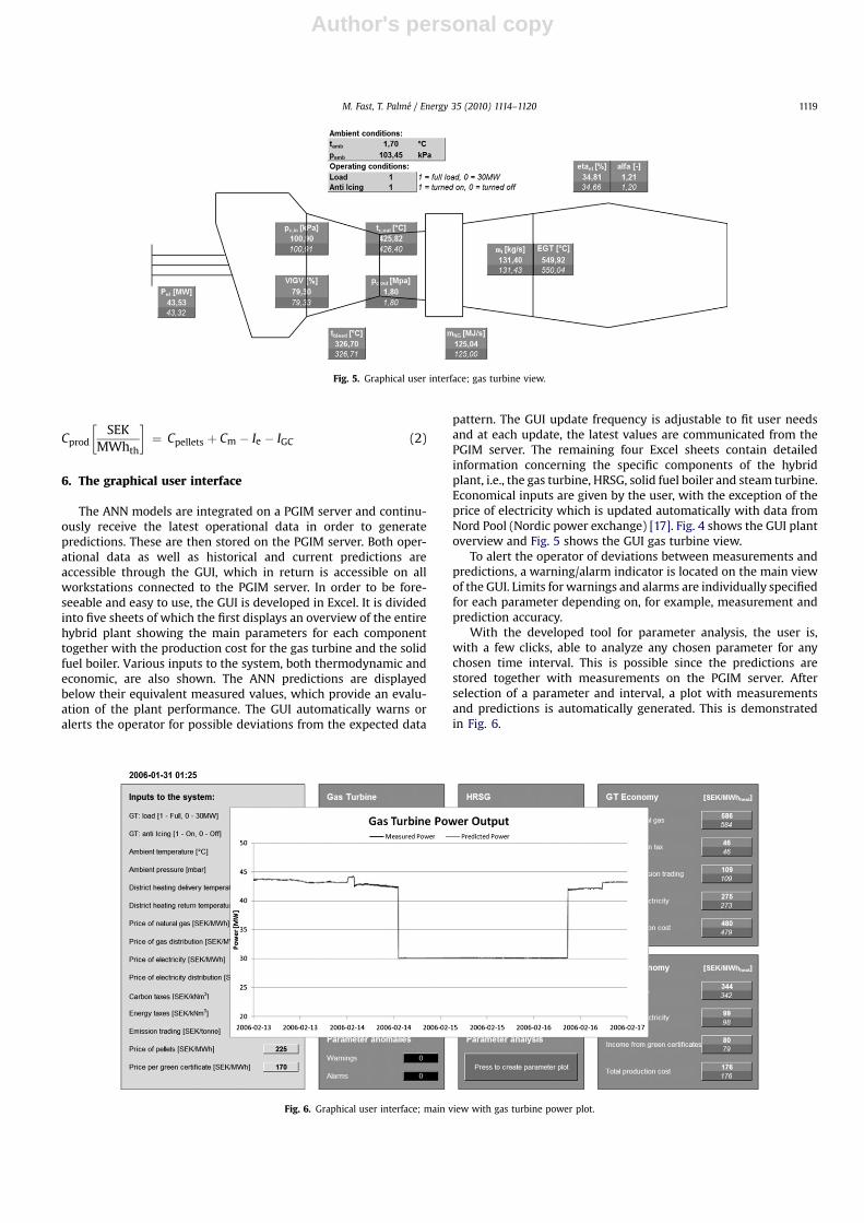
Author's personal copy

Cprod

�SEK

MWhth

�¼ Cpellets þ Cm � Ie � IGC (2)

6. The graphical user interface

The ANN models are integrated on a PGIM server and continu-ously receive the latest operational data in order to generatepredictions. These are then stored on the PGIM server. Both oper-ational data as well as historical and current predictions areaccessible through the GUI, which in return is accessible on allworkstations connected to the PGIM server. In order to be fore-seeable and easy to use, the GUI is developed in Excel. It is dividedinto five sheets of which the first displays an overview of the entirehybrid plant showing the main parameters for each componenttogether with the production cost for the gas turbine and the solidfuel boiler. Various inputs to the system, both thermodynamic andeconomic, are also shown. The ANN predictions are displayedbelow their equivalent measured values, which provide an evalu-ation of the plant performance. The GUI automatically warns oralerts the operator for possible deviations from the expected data

pattern. The GUI update frequency is adjustable to fit user needsand at each update, the latest values are communicated from thePGIM server. The remaining four Excel sheets contain detailedinformation concerning the specific components of the hybridplant, i.e., the gas turbine, HRSG, solid fuel boiler and steam turbine.Economical inputs are given by the user, with the exception of theprice of electricity which is updated automatically with data fromNord Pool (Nordic power exchange) [17]. Fig. 4 shows the GUI plantoverview and Fig. 5 shows the GUI gas turbine view.

To alert the operator of deviations between measurements andpredictions, a warning/alarm indicator is located on the main viewof the GUI. Limits for warnings and alarms are individually specifiedfor each parameter depending on, for example, measurement andprediction accuracy.

With the developed tool for parameter analysis, the user is,with a few clicks, able to analyze any chosen parameter for anychosen time interval. This is possible since the predictions arestored together with measurements on the PGIM server. Afterselection of a parameter and interval, a plot with measurementsand predictions is automatically generated. This is demonstratedin Fig. 6.

Fig. 5. Graphical user interface; gas turbine view.

Fig. 6. Graphical user interface; main view with gas turbine power plot.

M. Fast, T. Palme / Energy 35 (2010) 1114–1120 1119

Author's personal copy

7. Conclusions

The present study has demonstrated that ANN modeling of allthe major CHP plant components is possible. With proper training,data and parameter selection, it is also feasible to achieve very highprediction accuracies. It was shown that a real product, for onlinecondition monitoring, can be developed and integrated on-site,using an artificial neural network. The graphical user interface wasaccessible through all workstations connected to the internalnetwork, providing a capacity for online monitoring over the entiresite. With the developed tool, the condition of a plant could thus bemonitored while simultaneously economically evaluating possibledeviations, such as degradation or faults. Hence, by using thedeveloped tool, an optimization of the plant operation and main-tenance was rendered possible.

The described ANN models are plant specific; however, themethod is general and thereby applicable to other power plants andpower plant configurations.

Acknowledgements

The funders of this project, the Swedish Gas Center AB (SGC) andVarmeforsk AB, are greatly acknowledged. Siemens IndustrialTurbomachinery AB and Oresundskraft AB are also greatlyacknowledged for their assistance regarding gas turbine, powerplant and computer system related matters.

References

[1] Cerri G, Borghetti S, Salvini C. Neural management for heat and powercogeneration plants. Engineering Application of Artificial Intelligence2006;19:721–30.

[2] Weerasinghe M, Gomm JB, Williams D. Neural networks for fault diagnosis ofa nuclear fuel processing plant at different operating points. Control Engi-neering Practice 1998;6:281–9.

[3] Joly RB, Ogaji SOT, Singh R, Propert SD. Gas-turbine diagnostics using artificialneural-networks for a high bypass military turbofan engine. Applied Energy2004;78:397–418.

[4] Simani S, Fantuzzi C. Fault diagnosis in power plant using neural networks.Information Sciences 2000;127:125–36.

[5] Arriagada J, Genrup M, Loberg A, Assadi M. Fault diagnosis system for anindustrial gas turbine by means of neural networks. Tokyo: IGTC; 2003.

[6] De S, Kaiadi M, Fast M, Assadi M. Development of an artificial neural networkmodel for the steam process of a coal biomass co-fired combined heat andpower (CHP) plant in Sweden. Energy 2007;32(11):2099–109.

[7] Fast M, Assadi M, De S. Development and multi-utility of an ANN model for anindustrial gas turbine. Applied Energy 2008;86(1):9–17.

[8] Fast M, De S, Assadi M. Condition based maintenance of gas turbines usingsimulation data and artificial neural network: a demonstration of feasibility.ASME Turbo Expo, 2008, Berlin.

[9] Hellberg C. Distribution of electricity and heat production between thepowder boiler and the heat recovery steam generator. [Fordelning av el- ochvarmeproduktion mellan pulverpannan och avgaspannan]. Master’s thesis. .Lund: Division of Thermal Power Engineering, Department of Energy Sciences,Lund University (P.O. Box 118, S-221 00); 2004 [in Swedish].

[10] Evaluation of gas turbine GTX100 in Helsingborg – Stage 1. [Utvardering avgasturbin GTX100 i Helsingborg – Etapp 1]. Report no. A31. Swedish GasCenter, See also: http://www.sgc.se/dokument/sgca31.pdf/; 2001 [in Swedish].

[11] Haykin S. Neural networks: a comprehensive foundation. 2nd Ed. New Jersey:Prentice Hall; 1999.

[12] Principe JC, Euliano NR, Lefebvre WC. Neural and adaptive systems. New York:John Wiley & Sons Inc.; 2000.

[13] Rumelhart DE, Hinton GE, Williams RJ. Learning internal representations byerror propagation. Parallel distributed processing: explorations in themicrostructure of cognition, vol. 1(1). Cambridge, MA: MIT Press; 1986.p. 318–362.

[14] Cybenko G. Approximation by superpositions of a sigmoidal function. Math-ematics of Control, Signals, and Systems (MCSS) 1989;2(4):303–14.

[15] Swedish Energy Agency. Eskilstuna, 2009. See also: http://www.energimyndigheten.se/.

[16] Montgomery WD. Markets in licenses and efficient pollution controlprograms. Economic Theory 1972;5(3):395–418.

[17] Nordic Power Exchange. 2009. See also: http://www.nordpool.com/en/.

M. Fast, T. Palme / Energy 35 (2010) 1114–11201120

Condition based maintenance of gas turbines using simulation data and

artificial neural network: A demonstration of feasibility Fast M, Assadi M, De S.

Presented at ASME Turbo Expo 2008, Berlin, Germany

Paper III

CONDITION BASED MAINTENANCE OF GAS TURBINES USING SIMULATION DATA AND ARTIFICIAL NEURAL NETWORK: A DEMONSTRATION OF FEASIBILITY

Magnus Fast Division of Thermal Power Engineering

Department of Energy Sciences Lund University

P.O. Box 118, S-221 00 Lund, Sweden

Mohsen Assadi Division of Thermal Power Engineering

Department of Energy Sciences Lund University

P.O. Box 118, S-221 00 Lund, Sweden

Sudipta De Department of Mechanical Engineering

Jadavpur University, Kolkata: 700032, India

Proceedings of ASME Turbo Expo 2008: Power for Land, Sea and Air GT2008

June 9-13, 2008, Berlin, Germany

GT2008-50768

ABSTRACT

Gas turbine maintenance is crucial due to high cost for the replacement of its components and associated loss of pow-er during shutdown period. Conventional scheduled mainten-ance, based on equivalent operating hours, is not the best al-ternative as it can require unnecessary shut downs. Condition based maintenance is an attractive alternative as it decreases unnecessary shut downs and has other advantages for both the manufacturers and the plant owners. However, this has shown to be a complex/difficult task. A number of methods and ap-proaches have been presented to develop condition monitoring tools during the past decade. Condition monitoring tools can e.g. be developed by means of training artificial neural net-works (ANN) with historical operational data. Such tools can be used for online gas turbine performance prediction where input data from the plant is fed directly to the trained ANN models. The predicted outputs from the models are compared with corresponding measurements and possible deviations are evaluated. With this method both recoverable degradation, caused by fouling, and irrecoverable degradation, caused by wear, can be detected and hence both compressor wash and overhaul periods optimized. However, non-availability of op-erational data at the beginning of the gas turbine operation may cause problems for the development of ANN based con-dition monitoring tools.

Simulation data, on the other hand, may be generated by using a manufacturer’s engine design program. This data can be used for training artificial neural networks to overcome

the problem of non-availability of operational data. ANN models trained with simulation data could be used to monitor the engine from the very beginning of its operation. A demon-stration case using a Siemens gas turbine has been shown for this proposed method by comparing two ANN models, one trained with operational data and the other with simulation data. For the comparison an arbitrary section of operational data was used to produce predictions from both models, whe-reupon these were plotted with corresponding measured data. The comparison shows that the trends are very similar but the parameter values for the measured and the simulated data are shifted by a constant. Using this knowledge, one can provide an ANN based engine monitoring tool that could be adjusted to a certain engine using engine performance test data. The study shows promising results and motivates further investiga-tions in this field. 1 INTRODUCTION

Gas turbines for power generation need continuous monitoring and proper maintenance as their sudden break downs may lead to heavy penalty both due to expensive spare parts and the production loss accumulated. This is even more stringent now under the changed scenario of deregulation of electricity. Conventionally original equipment manufacturers (OEM) recommend scheduled maintenance of gas turbines. Intervals of scheduled maintenance are based on the equiva-lent operating hours (EOH) [1]. Warranty of gas turbines is usually subjected to compliance of scheduled maintenance by

1 Copyright © 2008 by ASME

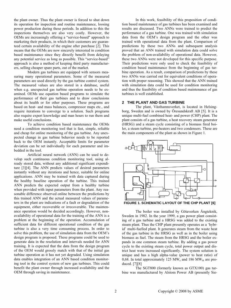
the plant owner. Thus the plant owner is forced to shut down its operation for inspection and routine maintenance, loosing power production during these periods. In addition to this the inspections themselves are also very costly. However, the OEMs are increasingly offering a “service-based" approach to marketing their products, in which their customers are guaran-teed certain availability of the engine after purchase [2]. This means that the OEMs are now sincerely interested in condition based maintenance since they directly benefit from delaying any potential service as long as possible. This “service-based” approach is also a method of keeping third party manufactur-ers, selling cheaper spare parts, out of the market.

Modern gas turbines are equipped with sensors mea-suring many operational parameters. Some of the measured parameters are used directly by the gas turbine control system. The measured values are also stored in a database, useful when e.g. unexpected gas turbine operation needs to be ex-amined. OEMs use equation based programs to simulate the performance of their gas turbines and to draw conclusions about its health or for other purposes. These programs are based on heat- and mass balances, compressor maps etc., and require iterations to converge to a solution. Such programs also require expert knowledge and man hours to run them and make useful conclusions.

To achieve condition based maintenance the OEMs need a condition monitoring tool that is fast, simple, reliable and cheap for online monitoring of the gas turbine. Any unex-pected change in gas turbine behavior needs to be reported back to the OEM instantly. Acceptable limits for parameter deviation can be set individually for each parameter and im-bedded in the tool.

Artificial neural network (ANN) can be used to de-velop such continuous condition monitoring tool, using al-ready stored data, without any additional significant expendi-ture [3][4]. The ANN predicts values of desired parameters instantly without any iterations and hence, suitable for online applications. ANN may be trained with data captured during the healthy baseline operation of the turbine. This trained ANN predicts the expected output from a healthy turbine when provided with input parameters from the plant. Any rea-sonable difference observed online between the predictions by this trained ANN and the actual measured values of parame-ters in the plant are indications of a fault or degradation of the equipment, either recoverable or irrecoverable. The mainten-ance operation would be decided accordingly. However, non-availability of operational data for the training of the ANN is a problem at the beginning of the operation. Accumulation of sufficient data for different operational condition of the gas turbine is also a very time consuming process. In order to solve this problem, the use of simulation data from the OEM’s design program is proposed. These programs could be used to generate data in the resolution and intervals needed for ANN training. It is expected that the data from the design program of the OEM would grossly match with that of the initial gas turbine operation as it has not yet degraded. Using simulation data enables integration of an ANN based condition monitor-ing tool in the control system of new gas turbines. This could benefit the plant owner through increased availability and the OEM through saving in maintenance.

2

In this work, feasibility of this proposition of condi-tion based maintenance of gas turbines has been examined and results are discussed. Two ANNs were trained to predict the performance of a gas turbine. One was trained with simulation data from the OEM’s design program and the other was trained with operational data from the plant. Comparison of predictions by these two ANNs and subsequent analysis proved that an ANN trained with simulation data could solve the problem of non-availability of operational data. However, these two ANNs were not developed for this specific purpose. Their predictions were only used to check the feasibility of condition based maintenance from the beginning of gas tur-bine operation. As a result, comparison of predictions by these two ANNs was carried out for equivalent conditions of opera-tion with proper reasoning. This showed that the ANN trained with simulation data could be used for condition monitoring and thus the feasibility of condition based maintenance of gas turbines is well established. 2 THE PLANT AND GAS TURBINE

The plant, Västhamnsverket, is located in Helsing-borg, Sweden and is owned by Öresundskraft AB [5]. It is a unique multi-fuel combined heat- and power (CHP) plant. The plant consists of a gas turbine, a heat recovery steam generator (HRSG) and a steam cycle consisting of a biomass fired boi-ler, a steam turbine, pre-heaters and two condensers. These are the main components of the plant as shown in Figure 1.

FIGURE 1. SCHEMATIC LAYOUT OF THE CHP PLANT [6]

The boiler was installed by Götaverken Ångteknik,

Sweden in 1982. In the year 1999, a gas power plant consist-ing of a gas turbine and a HRSG was added to the existing steam plant. Thus the CHP plant presently operates as a ‘hybr-id’ multi-fuelled plant. It generates steam from the waste heat of the gas turbine in the HRSG as well as in the boiler using biomass as fuel. The steam from the HRSG and the boiler ex-pands in one common steam turbine. By adding a gas power cycle to the existing steam cycle, total power output and dis-trict heat were increased significantly. The system solution is unique and has a high alpha-value (power to heat ratio) of 0,68. In total approximately 125 MWe and 186 MWth are pro-duced. [7][8]

The SGT800 (formerly known as GTX100) gas tur-bine was manufactured by Alstom Power AB (presently Sie-

Copyright © 2008 by ASME

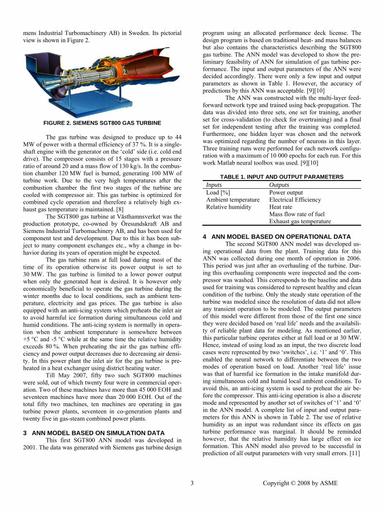
mens Industrial Turbomachinery AB) in Sweden. Its pictorial view is shown in Figure 2.

FIGURE 2. SIEMENS SGT800 GAS TURBINE

The gas turbine was designed to produce up to 44

MW of power with a thermal efficiency of 37 %. It is a single-shaft engine with the generator on the ‘cold’ side (i.e. cold end drive). The compressor consists of 15 stages with a pressure ratio of around 20 and a mass flow of 130 kg/s. In the combus-tion chamber 120 MW fuel is burned, generating 100 MW of turbine work. Due to the very high temperatures after the combustion chamber the first two stages of the turbine are cooled with compressor air. This gas turbine is optimized for combined cycle operation and therefore a relatively high ex-haust gas temperature is maintained. [8]

The SGT800 gas turbine at Västhamnsverket was the production prototype, co-owned by Öresundskraft AB and Siemens Industrial Turbomachinery AB, and has been used for component test and development. Due to this it has been sub-ject to many component exchanges etc., why a change in be-havior during its years of operation might be expected.

The gas turbine runs at full load during most of the time of its operation otherwise its power output is set to 30 MW. The gas turbine is limited to a lower power output when only the generated heat is desired. It is however only economically beneficial to operate the gas turbine during the winter months due to local conditions, such as ambient tem-perature, electricity and gas prices. The gas turbine is also equipped with an anti-icing system which preheats the inlet air to avoid harmful ice formation during simultaneous cold and humid conditions. The anti-icing system is normally in opera-tion when the ambient temperature is somewhere between +5 °C and -5 °C while at the same time the relative humidity exceeds 80 %. When preheating the air the gas turbine effi-ciency and power output decreases due to decreasing air densi-ty. In this power plant the inlet air for the gas turbine is pre-heated in a heat exchanger using district heating water.

Till May 2007, fifty two such SGT800 machines were sold, out of which twenty four were in commercial oper-ation. Two of these machines have more than 45 000 EOH and seventeen machines have more than 20 000 EOH. Out of the total fifty two machines, ten machines are operating in gas turbine power plants, seventeen in co-generation plants and twenty five in gas-steam combined power plants. 3 ANN MODEL BASED ON SIMULATION DATA

This first SGT800 ANN model was developed in 2001. The data was generated with Siemens gas turbine design

3

program using an allocated performance deck license. The design program is based on traditional heat- and mass balances but also contains the characteristics describing the SGT800 gas turbine. The ANN model was developed to show the pre-liminary feasibility of ANN for simulation of gas turbine per-formance. The input and output parameters of the ANN were decided accordingly. There were only a few input and output parameters as shown in Table 1. However, the accuracy of predictions by this ANN was acceptable. [9][10] The ANN was constructed with the multi-layer feed-forward network type and trained using back-propagation. The data was divided into three sets, one set for training, another set for cross-validation (to check for overtraining) and a final set for independent testing after the training was completed. Furthermore, one hidden layer was chosen and the network was optimized regarding the number of neurons in this layer. Three training runs were performed for each network configu-ration with a maximum of 10 000 epochs for each run. For this work Matlab neural toolbox was used. [9][10]

TABLE 1. INPUT AND OUTPUT PARAMETERS Inputs Outputs Load [%] Power output Ambient temperature Electrical Efficiency Relative humidity Heat rate Mass flow rate of fuel Exhaust gas temperature

4 ANN MODEL BASED ON OPERATIONAL DATA

The second SGT800 ANN model was developed us-ing operational data from the plant. Training data for this ANN was collected during one month of operation in 2006. This period was just after an overhauling of the turbine. Dur-ing this overhauling components were inspected and the com-pressor was washed. This corresponds to the baseline and data used for training was considered to represent healthy and clean condition of the turbine. Only the steady state operation of the turbine was modeled since the resolution of data did not allow any transient operation to be modeled. The output parameters of this model were different from those of the first one since they were decided based on ‘real life’ needs and the availabili-ty of reliable plant data for modeling. As mentioned earlier, this particular turbine operates either at full load or at 30 MW. Hence, instead of using load as an input, the two discrete load cases were represented by two ‘switches’, i.e. ‘1’ and ‘0’. This enabled the neural network to differentiate between the two modes of operation based on load. Another ‘real life’ issue was that of harmful ice formation in the intake manifold dur-ing simultaneous cold and humid local ambient conditions. To avoid this, an anti-icing system is used to preheat the air be-fore the compressor. This anti-icing operation is also a discrete mode and represented by another set of switches of ‘1’ and ‘0’ in the ANN model. A complete list of input and output para-meters for this ANN is shown in Table 2. The use of relative humidity as an input was redundant since its effects on gas turbine performance was marginal. It should be reminded however, that the relative humidity has large effect on ice formation. This ANN model also proved to be successful in prediction of all output parameters with very small errors. [11]

Copyright © 2008 by ASME

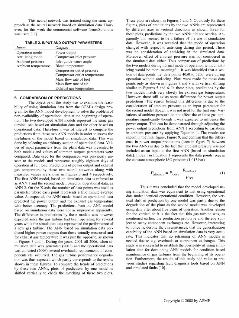
This neural network was trained using the same ap-proach as the neural network based on simulation data. How-ever, for this work the commercial software NeuroSolutions was used. [11]

TABLE 2. INPUT AND OUTPUT PARAMETERS Inputs Outputs Operation mode Power output Anti-icing mode Compressor inlet pressure Ambient pressure Inlet guide vanes angle Ambient temperature Bleed temperature Compressor outlet pressure Compressor outlet temperature Mass flow rate of fuel Mass flow rate of air Exhaust gas temperature

5 COMPARISON OF PREDICTIONS

The objective of this study was to examine the feasi-bility of using simulation data from the OEM’s design pro-gram for the ANN model development to solve the problem of non-availability of operational data at the beginning of opera-tion. The two developed ANN models represent the same gas turbine, one based on simulation data and the other based on operational data. Therefore it was of interest to compare the predictions from these two ANN models in order to assess the usefulness of the model based on simulation data. This was done by selecting an arbitrary section of operational data. Val-ues of input parameters from the plant data was presented to both models and values of common outputs parameters were compared. Data used for the comparison was previously un-seen to the models and represents roughly eighteen days of operation at full load. Predictions of power output and exhaust gas temperature by these two neural networks along with measured values are shown in Figures 3 and 4 respectively. The first ANN model, based on simulation data is referred to as ANN 1 and the second model, based on operational data, as ANN 2. On the X-axis the number of data points was used as parameter where each point represents a five minute average value. As expected, the ANN model based on operational data predicted the power output and the exhaust gas temperature with better accuracy. The predictions from the ANN model based on simulation data were not as impressive apparently. The difference in predictions by these models was however expected since the gas turbine had been operating for several years while the simulation data represented the performance of a new gas turbine. The ANN based on simulation data pre-dicted higher power outputs than those actually measured and for exhaust gas temperature it was just the opposite, as shown in Figures 3 and 4. During the years, 2001 till 2006, when si-mulation data was generated (2001) and the operational data was collected (2006) several overhauls, replacements of com-ponents etc. occurred. The gas turbine performance degrada-tion was thus expected which partly corresponds to the results shown in these figures. To compare the trends of predictions by these two ANNs, plots of predictions by one model is shifted vertically to check the matching of these two plots.

4

These plots are shown in Figures 5 and 6. Obviously for these figures, plots of predictions by the two ANNs are represented by different axes in vertical directions as shown. Even for these plots, predictions by the two ANNs did not overlap. Ap-parently this seemed to be a failure of the use of simulation data. However, it was revealed that the mode of operation changed with respect to anti-icing during this period. There was no consideration of anti-icing in the simulated data. Moreover, effect of ambient pressure was not considered in the simulated data either. Thus comparison of predictions by the two models during normal mode of operation without anti-icing would be more meaningful. It was identified that a sec-tion of data points, i.e. data points 4050 to 5200, were during operation without anti-icing. Plots were made for these data points only as shown in Figures 7 and 8 with vertical shifting similar to Figures 5 and 6. In these plots, predictions by the two models match very closely for exhaust gas temperature. However, there still exists some difference for power output predictions. The reason behind this difference is due to the consideration of ambient pressure as an input parameter for the second model though it was not used for the first one. Var-iations of ambient pressure do not affect the exhaust gas tem-perature significantly though it was expected to influence the power output. This can be demonstrated through adjusting the power output predictions from ANN 1 according to variations in ambient pressure by applying Equation 1. The results are shown in the final figure, Figure 9, and confirm that the differ-ence in power output predictions (seen in figure 7) between the two ANNs is due to the fact that ambient pressure was not included as an input to the first ANN (based on simulation data). Index i in Equation 1 represents the data points, pISO is the constant atmospheric ISO pressure (1,013 bar).

ISO

iambientiANNiadjusted p

pPP ,

,, ⋅= (1)

Thus it was concluded that the model developed us-

ing simulation data was equivalent to that using operational data under identical operational condition. However, the ver-tical shift in prediction by one model was partly due to the degradation of the plant as the second model was developed using data after about five years of operation. Another reason for the vertical shift is the fact that this gas turbine was, as mentioned earlier, the production prototype and thereby sub-ject to many component exchanges etc. However, interesting to notice is, despite the circumstances, that the generalization capability of the ANN based on simulation data is very accu-rate. This indicates that no retraining of ANN models is needed due to e.g. overhauls or component exchanges. This study was successful to establish the possibility of using simu-lation data for developing ANN models for condition based maintenance of gas turbines from the beginning of its opera-tion. Furthermore, the results of this study add value to pre-vious studies regarding fault diagnosis tools based on ANN and simulated faults [10].

Copyright © 2008 by ASME

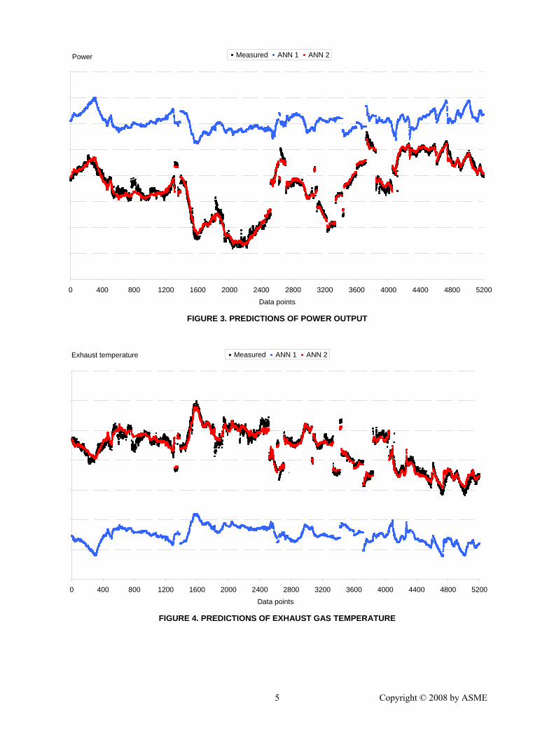
0,86

0,88

0,9

0,92

0,94

0,96

0,98

1

1,02

0 400 800 1200 1600 2000 2400 2800 3200 3600 4000 4400 4800 5200

Data points

Power Measured ANN 1 ANN 2

FIGURE 3. PREDICTIONS OF POWER OUTPUT

0,97

0,975

0,98

0,985

0,99

0,995

1

1,005

0 400 800 1200 1600 2000 2400 2800 3200 3600 4000 4400 4800 5200

Data points

Exhaust temperature Measured ANN 1 ANN 2

'

FIGURE 4. PREDICTIONS OF EXHAUST GAS TEMPERATURE

5 Copyright © 2008 by ASME

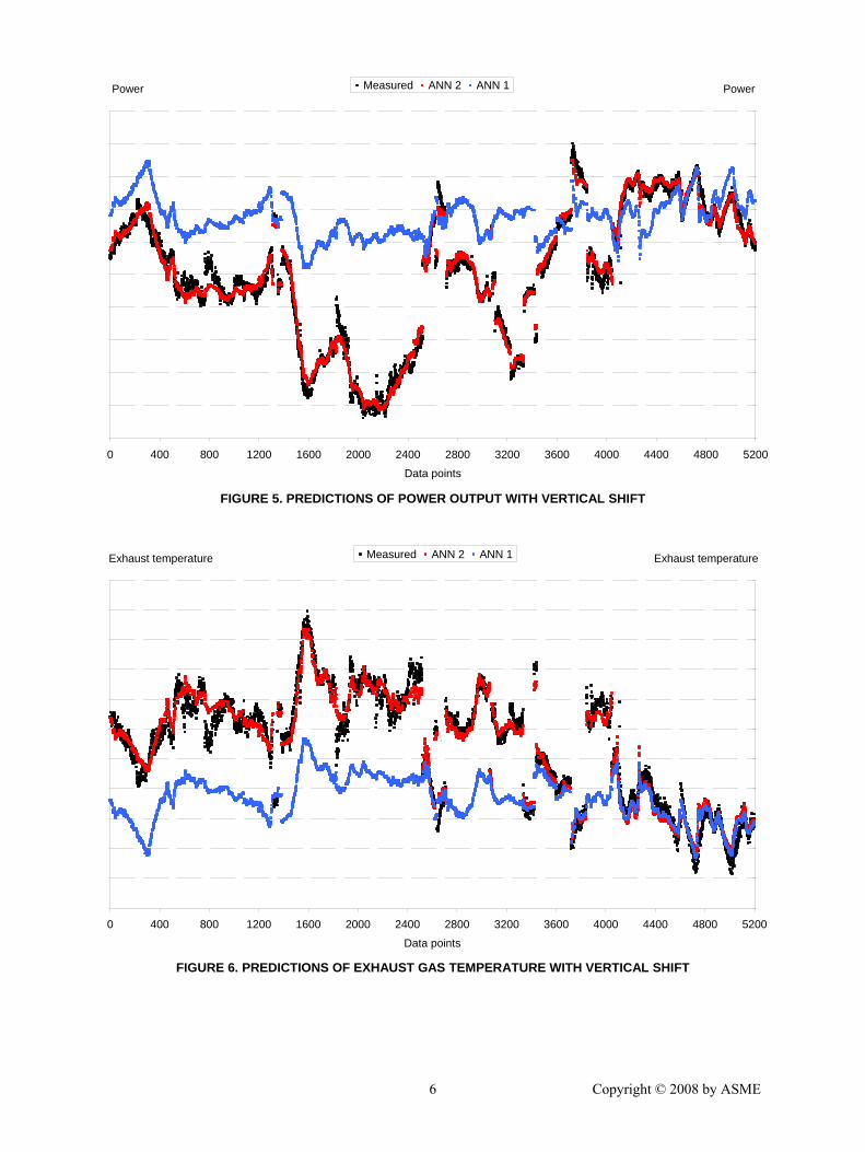
41

41,5

42

42,5

43

43,5

44

44,5

45

45,5

46

0 400 800 1200 1600 2000 2400 2800 3200 3600 4000 4400 4800 5200

Data points

Power

42,5

43

43,5

44

44,5

45

45,5

46

46,5

47

47,5

PowerMeasured ANN 2 ANN 1

FIGURE 5. PREDICTIONS OF POWER OUTPUT WITH VERTICAL SHIFT

543

544

545

546

547

548

549

550

551

552

553

554

0 400 800 1200 1600 2000 2400 2800 3200 3600 4000 4400 4800 5200

Data points

Exhaust temperature

536,8

537,8

538,8

539,8

540,8

541,8

542,8

543,8

544,8

545,8

546,8

547,8

Exhaust temperatureMeasured ANN 2 ANN 1

'

FIGURE 6. PREDICTIONS OF EXHAUST GAS TEMPERATURE WITH VERTICAL SHIFT

6 Copyright © 2008 by ASME

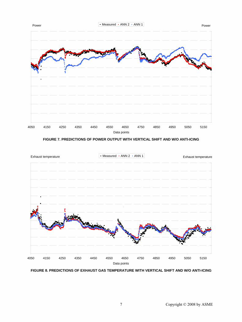
41

41,5

42

42,5

43

43,5

44

44,5

45

45,5

46

4050 4150 4250 4350 4450 4550 4650 4750 4850 4950 5050 5150

Data points

Power

42,5

43

43,5

44

44,5

45

45,5

46

46,5

47

47,5

PowerMeasured ANN 2 ANN 1

FIGURE 7. PREDICTIONS OF POWER OUTPUT WITH VERTICAL SHIFT AND W/O ANTI-ICING

543

544

545

546

547

548

549

550

551

552

553

554

4050 4150 4250 4350 4450 4550 4650 4750 4850 4950 5050 5150

Data points

Exhaust temperature

536,8

537,8

538,8

539,8

540,8

541,8

542,8

543,8

544,8

545,8

546,8

547,8

Exhaust temperatureMeasured ANN 2 ANN 1

'

FIGURE 8. PREDICTIONS OF EXHAUST GAS TEMPERATURE WITH VERTICAL SHIFT AND W/O ANTI-ICING

7 Copyright © 2008 by ASME

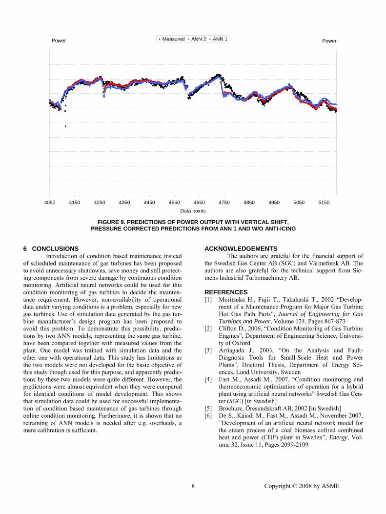
41

41,5

42

42,5

43

43,5

44

44,5

45

45,5

46

4050 4150 4250 4350 4450 4550 4650 4750 4850 4950 5050 5150

Data points

Power

42,5

43,13

43,76

44,39

45,02

45,65

46,28

46,91

47,54

48,17

48,8

PowerMeasured ANN 2 ANN 1

FIGURE 9. PREDICTIONS OF POWER OUTPUT WITH VERTICAL SHIFT,

PRESSURE CORRECTED PREDICTIONS FROM ANN 1 AND W/O ANTI-ICING

6 CONCLUSIONS Introduction of condition based maintenance instead

of scheduled maintenance of gas turbines has been proposed to avoid unnecessary shutdowns, save money and still protect-ing components from severe damage by continuous condition monitoring. Artificial neural networks could be used for this condition monitoring of gas turbines to decide the mainten-ance requirement. However, non-availability of operational data under varying conditions is a problem, especially for new gas turbines. Use of simulation data generated by the gas tur-bine manufacturer’s design program has been proposed to avoid this problem. To demonstrate this possibility, predic-tions by two ANN models, representing the same gas turbine, have been compared together with measured values from the plant. One model was trained with simulation data and the other one with operational data. This study has limitations as the two models were not developed for the basic objective of this study though used for this purpose, and apparently predic-tions by these two models were quite different. However, the predictions were almost equivalent when they were compared for identical conditions of model development. This shows that simulation data could be used for successful implementa-tion of condition based maintenance of gas turbines through online condition monitoring. Furthermore, it is shown that no retraining of ANN models is needed after e.g. overhauls, a mere calibration is sufficient.

ACKNOWLEDGEMENTS

The authors are grateful for the financial support of the Swedish Gas Center AB (SGC) and Värmeforsk AB. The authors are also grateful for the technical support from Sie-mens Industrial Turbomachinery AB. REFERENCES [1] Moritsuka H., Fujii T., Takahashi T., 2002 “Develop-

ment of a Maintenance Program for Major Gas Turbine Hot Gas Path Parts”, Journal of Engineering for Gas Turbines and Power, Volume 124, Pages 867-873

[2] Clifton D., 2006, “Condition Monitoring of Gas Turbine Engines”, Department of Engineering Science, Universi-ty of Oxford

[3] Arriagada J., 2003, “On the Analysis and Fault-Diagnosis Tools for Small-Scale Heat and Power Plants”, Doctoral Thesis, Department of Energy Sci-ences, Lund University, Sweden

[4] Fast M., Assadi M., 2007, “Condition monitoring and thermoeconomic optimization of operation for a hybrid plant using artificial neural networks” Swedish Gas Cen-ter (SGC) [in Swedish]

[5] Brochure, Öresundskraft AB, 2002 [in Swedish] [6] De S., Kaiadi M., Fast M., Assadi M., November 2007,

”Development of an artificial neural network model for the steam process of a coal biomass cofired combined heat and power (CHP) plant in Sweden”, Energy, Vol-ume 32, Issue 11, Pages 2099-2109

8 Copyright © 2008 by ASME

[7] Hellberg C., 2004, ”Distribution of electricity- and heat production between the powder boiler and the heat re-covery steam generator”, Masters thesis, Department of Energy Sciences, Lund University, Sweden [in Swedish]

[8] Torisson T., Assadi M., 2001, “Evaluation of gas turbine GTX100 in Helsingborg – Stage 1”, Swedish Gas Center (SGC) report no. A31 [in Swedish]

[9] Olausson P., Arriagada J., 2001, “Case study for evalua-tion of an ANN-model generated in Matlab Neural Toolbox, applied to GTX100”, Department of Energy Sciences, Lund University, Sweden

[10] Arriagada J., Genrup M., Loberg A., Assadi M., 2003, ”Fault Diagnosis System for an Industrial Gas Turbine by Means of Neural Networks”, IGTC, Tokyo, Japan.

[11] Fast M., Assadi M., 2006, ”ANN modeling for monitor-ing of a hybrid plant”, Swedish Gas Center (SGC) report no. 171 [in Swedish]

9 Copyright © 2008 by ASME

A novel approach for gas turbine monitoring combining CUSUM technique and artificial neural network

Fast M, Palmé T, Genrup M. Presented at ASME Turbo Expo 2009, Orlando, Florida, USA

Paper IV

Proceedings of ASME Turbo Expo 2009: Power for Land, Sea and Air GT2009

June 8-12, 2009, Orlando, Florida, USA

GT2009-59402

A NOVEL APPROACH FOR GAS TURBINE CONDITION MONITORING COMBINING CUSUM TECHNIQUE AND ARTIFICIAL NEURAL NETWORK

Magnus Fast Division of Thermal Power Engineering

Department of Energy Sciences Lund University

P.O. Box 118, S-221 00 Lund, Sweden

Thomas Palmé Department of Mechanical and Structural Engineering and

Materials Science University of Stavanger

N-4036 Stavanger, Norway

Magnus Genrup Division of Thermal Power Engineering

Department of Energy Sciences Lund University

P.O. Box 118, S-221 00 Lund, Sweden ABSTRACT Investigation of a novel condition monitoring approach, combining artificial neural network (ANN) with a sequential analysis technique, has been reported in this paper. For this purpose operational data from a Siemens SGT600 gas turbine has been employed for the training of an ANN model. This ANN model is subsequently used for the prediction of performance parameters of the gas turbine. Simulated anomalies are introduced on two different sets of operational data, acquired one year apart, whereupon this data is compared with corresponding ANN predictions. The cumulative sum (CUSUM) technique is used to improve and facilitate the detection of such anomalies in the gas turbine’s performance. The results are promising, displaying fast detection of small changes and detection of changes even for a degraded gas turbine. Keywords: ANN, CUSUM, condition monitoring, gas turbine 1 INTRODUCTION A steadily increasing demand for effective and reliable gas turbine condition monitoring systems, as a means to increase the availability and reliability, has lately forced the original equipment manufacturers (OEMs) to, at least, offer such systems together with their engines. These systems are most often developed from the OEMs engine performance decks, which are equation based iterative solvers comprising engine component maps etc. However, there is a reluctance to

disseminate source codes and maps at the same time as equation based iterative solvers might not be the best alternative for online tasks. Alternative approaches, using e.g., intelligent tools such as artificial neural network (ANN), have been investigated and evaluated for quite some time, with positive results. Researchers at the division of Thermal Power Engineering at Lund University have carried out several investigations [1-7] in this field and ANN has shown to be a good candidate for modeling of non-linear systems in the energy field and this work is a continuation of those previous studies.

ANN is strictly numerical and can be trained to recognize patterns using either operational data [4], from an actual engine, or simulation data, from an OEMs performance deck [7]. A trained ANN model is very small, due to its parallel structure, simple and consists only of straight forward equations, transferable into any programming language. The information is stored in the network’s weights, which consists of decimal numbers, and therefore no information about the gas turbine’s configuration is revealed. It is possible to achieve very high predictive performance with a properly configured and trained ANN using good quality data representing a broad range of operation. The predictions from an ANN model represents expected behavior of a gas turbine and can be continuously compared with corresponding measurements to detect any unexpected change, viz., condition monitoring. In this paper a technique is proposed to improve the detection of such changes by employing the CUSUM method. CUSUM

Copyright © 2009 by ASME 1

stands for cumulative sum and is a sequential analysis technique used for change detection purposes. By employing the CUSUM for change detection an ANN based condition monitoring tool can be better utilized through earlier detection of unwanted change in operation. Furthermore, an ANN model trained with operational data is tailored to a specific engine while an ANN model trained with simulation data is a more general representation of the engine type since all engines have their individualities. However, even when training an ANN with operational data, over time a level shift will appear between the predictions and measured values, due to degradation. This level shift, present from the beginning or developed over time, can complicate the change detection and would normally require a calibration or retraining of the ANN model. By employing the CUSUM method, calibration and retraining may prove unnecessary, since change detection is possible through studying directional changes of the cumulative sum instead of the actual values. In this paper an ANN is trained with operational data from a Siemens SGT600 gas turbine whereupon the proposed method is evaluated. 2 BRIEF BASICS OF ANN ANN is a non-linear statistical data modeling tool that basically learns from experience (i.e., adaptive) [8]. Instead of being built a priori from specification, neural and adaptive systems use external data to automatically set their parameters [9]. ANN can be used to solve a variety of tasks, including classification, regression, general estimations problems, etc. An ANN consists of a group of interconnected artificial neurons processing information in parallel. The performance of a network can be improved by rendering it “aware” of its output(s) through a performance feedback loop that includes a cost function. The feedback is used to adjust the network parameters through systematic procedures called learning or training rules, in order to improve the system output with respect to the desired goal [9].

The most common feedback algorithm is the back-propagation algorithm, proposed by Rumelhart et al. in 1986 [10], which provides a computationally efficient method for evaluation of the error function associated to each weight. The updating algorithm is based on a gradient descent method, where the updating algorithm updates the weights in order to minimize the error function. The multi-layer feed-forward network, more specifically the multi-layer perceptron (MLP), is the type of network which has been used during this study. It consists of an input layer, one or more hidden layer(s) and an output layer. However, there is no impediment to having more than one hidden layer, since it has been proven that one layer with hidden neurons is enough to approximate any continuous function if it only has a sufficient number of neurons [11]. Once the inputs are presented to the network they will be multiplied by their adjustable weights and in each processing element summed and passed through a transfer function in order to produce outputs. The data used as inputs is transmitted through the network, layer by layer, and a set of outputs is obtained. Errors are generated by comparing these outputs with the desired outputs. The errors are then used for updating the weights before another set of inputs is transmitted through the network, i.e., supervised training. The mean

squared error (MSE) is calculated between each epoch (iteration) and the training is terminated when the MSE is satisfactory low. When the training is completed the weights are fixed and the network is ready to predict outputs from previously unseen data, i.e., generalization.

Before commencement of the training process the data set is randomized and divided into three subsets, training, cross-validation and test set. The training set is used by the network for weight adjustment (i.e., learning) and the cross-validation set is used to avoid overtraining by the network. The test set is used after the training to ensure that good generalization capability is obtained. A properly trained network displays similar prediction errors, or accuracy, in all three data sets.

Even though ANN is adaptive, the actual network configuration has to be specified. Selection of the number of hidden neurons is carried out by a trial- and error procedure where the network is trained multiple times with different number of neurons in the hidden layer. The network exhibiting the highest prediction accuracy, in all three data sets, is selected. The number of neurons needed in the hidden layer is determined by the complexity of the input/output parameter dimension. It is preferable to select as few neurons as possible, without sacrificing the prediction accuracy, to provide good generalization capabilities. Each neuron includes a transfer function, in which the incoming data is processed. In this study, based on accumulated experience at the division, the tangent hyperbolic function is used as transfer function. 3 BASIC PRINCIPLES OF THE CUSUM TECHNIQUE The CUSUM technique was first proposed by Page [12] in 1954, for use in industrial process control to detect deviations in production parameters from pre-determined values. Before motivation of the CUSUM algorithm, the standard Shewhart control chart is introduced.

In the statistical theory, control charts are widely used to detect a shift in the mean value from a process, the most common are the Shewhart control charts [13]. The main goal with these charts is to distinguish natural variation from unnatural behavior. Several types of control charts exists, e.g., the “X chart” which is used for controlling central tendency and the “R chart” (or σ chart) which is used for controlling variability. If a variable is normally distributed, with the mean x and the standard deviation σ, the probability that xi will fall within the interval [x - 3σ, x + 3σ] is 0.9973. If instead a subgroup of n observations is considered, the new interval will be [x - 3σ/√n, x + 3σ/√n]. If a change between the expected and measured value occurs, the Shewhart charts provides a good detection tool. The major drawback of the Shewhart control charts is their inability to use the information contained in a sequence of plotted points. As a result, changes between the predicted mean and the measured mean are hard to detect if the change occurs inside the confidence limit set by the Shewhart chart.

The CUSUM technique was developed to solve the problem of detecting a change in a parameter, with emphasis on small changes. The main reason for detecting an unnatural behavior in a process is to provide a basis for action as soon as possible. In Engineering Statistics [13], two alternative types

Copyright © 2009 by ASME 2

of control charts are introduced with the purpose of using “past” knowledge. The first one is called signed sequential rank control chart (SSRCC) and the second cumulative sum control chart (CSCC), both of which have stopping rules that incorporate the information contained in all the sample points. This can be illustrated by considering a small shift in the mean value inside the upper and lower limits (the confidence limits) that may not be detected with the standard Shewhart charts. The CSCC is based on plotting the cumulative difference between the expected mean and the measured value for a parameter. The process is assumed to be in “control” as long as these points behave properly. Before the computational era, a detection chart called the V-mask was constructed in which failing data could be observed [13]. Good monitoring systems will take a long time before they indicate that an adjustment is necessary when the process is in control, i.e., an incorrect action, and take a short time to call for action when the process is no longer in control. This is measured by the average run length (ARL). A full explanation of how to calculate the ARL can be found in Engineering Statistics [13], which also provide a theoretical base for calculating the design parameters for the V-mask.

Several types of CUSUM algorithm are available and they all have their origin in the work proposed by Page [12]. In Detection of Abrupt Changes: Theory and Application [14] a description of the CUSUM algorithm used in offline and online applications is thoroughly discussed. In this study, an approach proposed by Lucas et al. [15] is used. This approach is fairly intuitive with few parameters to adjust for implementation. The first step is to compute the standardized deviations of observations from the desired process mean, shown in Eq (1. ).

(1)

Where xi is the observed value at time i, x is the

desired process mean and σ is an estimation of the standard deviation of the observed values. These are accumulated over time to compute the cumulative sum, S, at each time point i as seen in ). Eq. (2

,   0

(2)

If there is a shift in the process mean, zi will tend to be larger or smaller than the target and the CUSUM will either steadily increase or decrease. Depending on the magnitude of the shift in the mean value, the CUSUM will not detect the change immediately and will require a number of observations at the new level before the change in the mean is recognized. In Fast Initial Response for CUSUM Quality-Control Schemes [15] the authors proposed a pair of cumulative sums (see Eq. (3)) where the first is used for detecting an increase in the mean, and the second for detecting a decrease in the mean, the so calle tw tro chart. d o-sided CUSUM con l

max  0,min  0, (3)

The parameter k is a reference value or allowable slack in the process. A usual choice of k is 0.5 and is an appropriate choice when a shift of one standard deviation is desired to be detected in the process mean. The CUSUM chart includes lower and upper alarm limits, or confidence limits, of the magnitude ± hσ with h = 4 or 5. These limits are used as a means of differentiating between random changes and sustained changes in the mean value. It should be recognized that a CUSUM chart does not immediately detect a change in the mean, it requires a run of values at the new mean value before it indicates that a change has occurred. Four different parameters need to be specified in order to implement the algorithm. These include the standard deviation, the “batch” size of the process mean, the slack parameter and the confidence limits.

4 CASE STUDY The purpose of this case study is to investigate how the CUSUM technique can be advantageously employed, together with ANN, for the condition monitoring of a gas turbine. The investigation is twofold and the first step is to implement the CUSUM technique according to the theory explained in section 3. For this purpose operational data from a healthy and clean gas turbine, where ANN predictions and measurements match very closely, is employed. The second part of the study focuses on how the CUSUM technique can be employed if there is a level shift, between the ANN predictions and the measurements. For this purpose operational data is acquired from the same gas turbine after one year of operation. The second part is of certain interest since even if the monitoring tool, in this case an ANN model, have very high precision, over time a shift between this model and the actual machine will develop, due to degradation or component exchanges. It is not realistic to assume that the ANN model can be retrained every time this shift grows too large so the preferable scenario would be to have a monitoring system able to cope with this reality. An already developed and validated ANN model, representing clean and healthy performance of a SGT600 gas turbine individual, will be employed for this study. The performance predictions are compared with corresponding measurements and through introducing small errors on these measurements the CUSUM technique is evaluated. More specifically, a Siemens SGT600 machine (described in 4.1) is modeled with ANN (described in 4.2) and the use of the CUSUM technique is evaluated by comparing ANN predictions with a healthy gas turbine (described in 4.3) and also with the same gas turbine after some time of operation (described in 4.4). 4.1 The SGT600 Gas Turbine The power plant Gunnesboverket is owned by Lunds Energi AB and used for peak load operation during the winter months. It is a cogeneration plant consisting of a Siemens SGT600 gas turbine and a heat recovery unit connected to the district heating grid. The SGT600 gas turbine is a two-shaft unit and is thus suitable for both power generation and mechanical drive. The axial flow compressor has ten stages, of which the first two have a variable geometry, and generates a

Copyright © 2009 by ASME 3

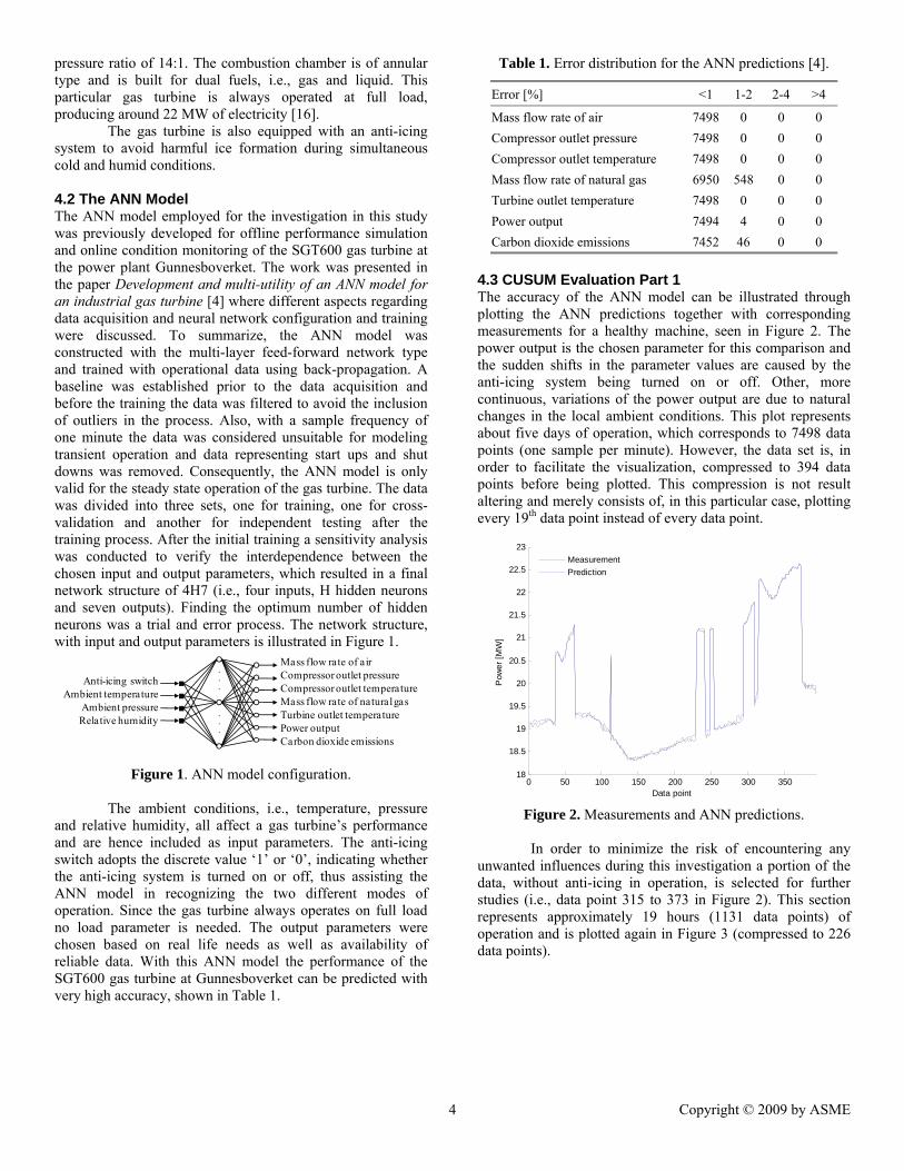
pressure ratio of 14:1. The combustion chamber is of annular type and is built for dual fuels, i.e., gas and liquid. This particular gas turbine is always operated at full load, producing around 22 MW of electricity [16].

The gas turbine is also equipped with an anti-icing system to avoid harmful ice formation during simultaneous cold and humid conditions. 4.2 The ANN Model The ANN model employed for the investigation in this study was previously developed for offline performance simulation and online condition monitoring of the SGT600 gas turbine at the power plant Gunnesboverket. The work was presented in the paper Development and multi-utility of an ANN model for an industrial gas turbine [4] where different aspects regarding data acquisition and neural network configuration and training were discussed. To summarize, the ANN model was constructed with the multi-layer feed-forward network type and trained with operational data using back-propagation. A baseline was established prior to the data acquisition and before the training the data was filtered to avoid the inclusion of outliers in the process. Also, with a sample frequency of one minute the data was considered unsuitable for modeling transient operation and data representing start ups and shut downs was removed. Consequently, the ANN model is only valid for the steady state operation of the gas turbine. The data was divided into three sets, one for training, one for cross-validation and another for independent testing after the training process. After the initial training a sensitivity analysis was conducted to verify the interdependence between the chosen input and output parameters, which resulted in a final network structure of 4H7 (i.e., four inputs, H hidden neurons and seven outputs). Finding the optimum number of hidden neurons was a trial and error process. The network structure, with input and output parameters is illustrated in Figure 1.

Figure 1. ANN model configuration.

The ambient conditions, i.e., temperature, pressure

and relative humidity, all affect a gas turbine’s performance and are hence included as input parameters. The anti-icing switch adopts the discrete value ‘1’ or ‘0’, indicating whether the anti-icing system is turned on or off, thus assisting the ANN model in recognizing the two different modes of operation. Since the gas turbine always operates on full load no load parameter is needed. The output parameters were chosen based on real life needs as well as availability of reliable data. With this ANN model the performance of the SGT600 gas turbine at Gunnesboverket can be predicted with very high accuracy, shown in Table 1.

Table 1. Error distribution for the ANN predictions [4].

Error [%] <1 1-2 2-4 >4

Mass flow rate of air 7498 0 0 0 Compressor outlet pressure 7498 0 0 0 Compressor outlet temperature 7498 0 0 0 Mass flow rate of natural gas 6950 548 0 0 Turbine outlet temperature 7498 0 0 0 Power output 7494 4 0 0 Carbon dioxide emissions 7452 46 0 0

4.3 CUSUM Evaluation Part 1 The accuracy of the ANN model can be illustrated through plotting the ANN predictions together with corresponding measurements for a healthy machine, seen in Figure 2. The power output is the chosen parameter for this comparison and the sudden shifts in the parameter values are caused by the anti-icing system being turned on or off. Other, more continuous, variations of the power output are due to natural changes in the local ambient conditions. This plot represents about five days of operation, which corresponds to 7498 data points (one sample per minute). However, the data set is, in order to facilitate the visualization, compressed to 394 data points before being plotted. This compression is not result altering and merely consists of, in this particular case, plotting every 19th data point instead of every data point.

Figure 2. Measurements and ANN predictions.

In order to minimize the risk of encountering any

unwanted influences during this investigation a portion of the data, without anti-icing in operation, is selected for further studies (i.e., data point 315 to 373 in Figure 2). This section represents approximately 19 hours (1131 data points) of operation and is plotted again in Figure 3 (compressed to 226 data points).

. . .. . .

Anti-icing switchAmbient temperature

Ambient pressureRelative humidity

Mass flow rate of airCompressor outlet pressureCompressor outlet temperatureMass flow rate of natural gasTurbine outlet temperaturePower outputCarbon dioxide emissions

0 50 100 150 200 250 300 35018

18.5

19

19.5

20

20.5

21

21.5

22

22.5

23

Data point

Pow

er [M

W]

MeasurementPrediction

Copyright © 2009 by ASME 4

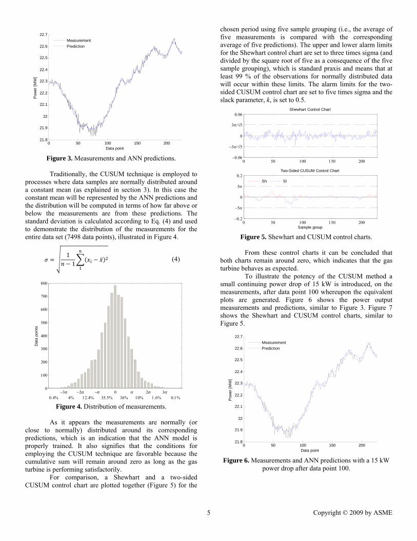
Figure 3. Measurements and ANN predictions.

Traditionally, the CUSUM technique is employed to

processes where data samples are normally distributed around a constant mean (as explained in section 3). In this case the constant mean will be represented by the ANN predictions and the distribution will be computed in terms of how far above or below the measurements are from these predictions. The standard deviation is calculated according to Eq. (4) and used to demonstrate the distribution of the measurements for the entire data set (7498 data points), illustrated in Figure 4.

11 (4)

Figure 4. Distribution of measurements.

As it appears the measurements are normally (or

close to normally) distributed around its corresponding predictions, which is an indication that the ANN model is properly trained. It also signifies that the conditions for employing the CUSUM technique are favorable because the cumulative sum will remain around zero as long as the gas turbine is performing satisfactorily.

For comparison, a Shewhart and a two-sided CUSUM control chart are plotted together (Figure 5) for the

chosen period using five sample grouping (i.e., the average of five measurements is compared with the corresponding average of five predictions). The upper and lower alarm limits for the Shewhart control chart are set to three times sigma (and divided by the square root of five as a consequence of the five sample grouping), which is standard praxis and means that at least 99 % of the observations for normally distributed data will occur within these limits. The alarm limits for the two-sided CUSUM control chart are set to five times sigma and the slack parameter, k, is set to 0.5.

Figure 5. Shewhart and CUSUM control charts.

From these control charts it can be concluded that

both charts remain around zero, which indicates that the gas turbine behaves as expected.

To illustrate the potency of the CUSUM method a small continuing power drop of 15 kW is introduced, on the measurements, after data point 100 whereupon the equivalent plots are generated. Figure 6 shows the power output measurements and predictions, similar to Figure 3. Figure 7 shows the Shewhart and CUSUM control charts, similar to Figure 5.

Figure 6. Measurements and ANN predictions with a 15 kW

power drop after data point 100.

0 50 100 150 20021.8

21.9

22

22.1

22.2

22.3

22.4

22.5

22.6

22.7

Data point

Pow

er [M

W]

MeasurementPrediction

−3σ −2σ −σ 0 σ 2σ 3σ0

100

200

300

400

500

600

700

800

Dat

a po

ints

0.4% 4% 12.4% 35.5% 36% 10% 1.6% 0.1%

0 50 100 150 200−0.06

−3σ/√5

0

3σ/√5

0.06Shewhart Control Chart

0 50 100 150 200−0.2

−5σ

0

5σ

0.2Two-Sided CUSUM Control Chart

Sample group

Sh Sl

0 50 100 150 20021.8

21.9

22

22.1

22.2

22.3

22.4

22.5

22.6

22.7

Data point

Pow

er [M

W]

MeasurementPrediction

Copyright © 2009 by ASME 5

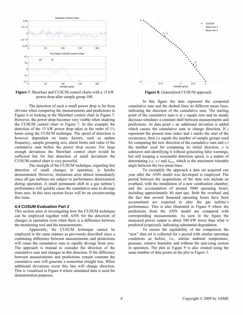
Figure 7. Shewhart and CUSUM control charts with a 15 kW

power drop after sample group 100.

The detection of such a small power drop is far from obvious when comparing the measurements and predictions in Figure 6 or looking at the Shewhart control chart in Figure 7. However, the power drop becomes very visible when studying the CUSUM control chart in Figure 7. In this example the detection of the 15 kW power drop takes in the order of 1½ hours using the CUSUM technique. The speed of detection is however dependant on many factors, such as update frequency, sample grouping size, alarm limits and value of the cumulative sum before the power drop occurs. For large enough deviations the Shewhart control chart would be sufficient but for fast detection of small deviations the CUSUM control chart is very powerful.

The strength of the CUSUM technique, regarding fast detection of small changes in operation, is hereby demonstrated. However, limitations arise almost immediately since all gas turbines are subject to performance deterioration during operation. A small permanent shift in a gas turbine’s performance will quickly cause the cumulative sum to diverge from zero. In this next section focus will be on circumventing this issue.

4.4 CUSUM Evaluation Part 2 This section aims at investigating how the CUSUM technique can be employed together with ANN for the detection of changes in operation even when there is a difference between the monitoring tool and the measurements.

Apparently, the CUSUM technique cannot be employed in the same manner as previously described since a continuing difference between measurements and predictions will cause the cumulative sum to rapidly diverge from zero. The approach is instead to consider the direction of the cumulative sum and changes in this direction. If the difference between measurements and predictions remain constant the cumulative sum will generate a somewhat straight line. When additional deviations occur this line will change direction. This is visualized in Figure 8 where simulated data is used for demonstration purposes.

Figure 8. Generalized CUSUM approach.

In this figure the dots represent the computed cumulative sum and the dashed lines its different mean lines, indicating the direction of the cumulative sum. The starting point of the cumulative sum is at y equals zero and its steady decrease simulates a constant shift between measurements and predictions. At data point x an additional deviation is added which causes the cumulative sum to change direction. If j represents the present time index and x marks the start of the occurrence, then j-x equals the number of sample groups used for computing the new direction of the cumulative sum and x-i the number used for computing its initial direction. x is unknown and identifying it without generating false warnings, but still keeping a reasonable detection speed, is a matter of determining j-x, x-i and δmax, which is the maximum tolerable angle between the two mean lines.

To exemplify the approach a data set acquired one year after the ANN model was developed is employed. The period between the acquisitions of the data sets include an overhaul, with the installation of a new combustion chamber, and the accumulation of around 5000 operating hours, including approximately 40 start ups. Both the overhaul and the fact that several thousand operating hours have been accumulated are expected to alter the gas turbine’s performance. This is also illustrated in Figure 9 where the predictions from the ANN model are compared with corresponding measurements. As seen in the figure the measured power output is about 500 kW lower than what is predicted (expected), indicating substantial degradation.

To ensure the equitability of the comparison the “new” data set is collected for a period with similar operating conditions as before, i.e., similar ambient temperature, pressure, relative humidity and without the anti-icing system in operation. The plot in Figure 9 is also created using the same number of data points as the plot in Figure 3.

0 50 100 150 200−0.06

−3σ/√5

0

3σ/√5

0.06Shewhart Control Chart

0 50 100 150 200−0.2

−5σ

0

5σ

0.2Two-Sided CUSUM Control Chart

Sample group

Sh Sl

i (x-i) x (j-x) j-y

0

Sample group

CUSUMMean line 1Mean line 2

δ

δ

Copyright © 2009 by ASME 6

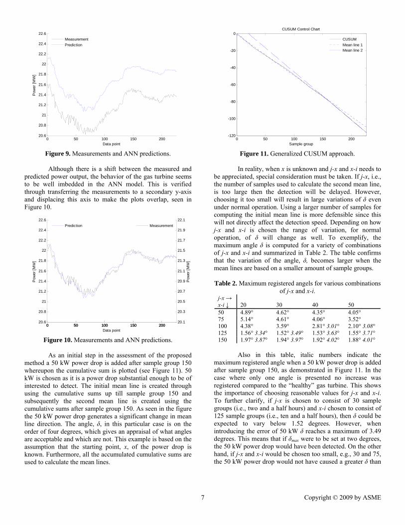
Figure 9. Measurements and ANN predictions. Although there is a shift between the measured and

predicted power output, the behavior of the gas turbine seems to be well imbedded in the ANN model. This is verified through transferring the measurements to a secondary y-axis and displacing this axis to make the plots overlap, seen in Figure 10.

Figure 10. Measurements and ANN predictions.

As an initial step in the assessment of the proposed

method a 50 kW power drop is added after sample group 150 whereupon the cumulative sum is plotted (see Figure 11). 50 kW is chosen as it is a power drop substantial enough to be of interested to detect. The initial mean line is created through using the cumulative sums up till sample group 150 and subsequently the second mean line is created using the cumulative sums after sample group 150. As seen in the figure the 50 kW power drop generates a significant change in mean line direction. The angle, δ, in this particular case is on the order of four degrees, which gives an appraisal of what angles are acceptable and which are not. This example is based on the assumption that the starting point, x, of the power drop is known. Furthermore, all the accumulated cumulative sums are used to calculate the mean lines.

Figure 11. Generalized CUSUM approach.

In reality, when x is unknown and j-x and x-i needs to

be appreciated, special consideration must be taken. If j-x, i.e., the number of samples used to calculate the second mean line, is too large then the detection will be delayed. However, choosing it too small will result in large variations of δ even under normal operation. Using a larger number of samples for computing the initial mean line is more defensible since this will not directly affect the detection speed. Depending on how j-x and x-i is chosen the range of variation, for normal operation, of δ will change as well. To exemplify, the maximum angle δ is computed for a variety of combinations of j-x and x-i and summarized in Table 2. The table confirms that the variation of the angle, δ, becomes larger when the mean lines are based on a smaller amount of sample groups.

Table 2. Maximum registered angels for various combinations

of j-x and x-i. j-x → x-i ↓

20

30

40

50

50 4.89° 4.62° 4.35° 4.05° 75 5.14° 4.61° 4.06° 3.52° 100 4.38° 3.59° 2.81° 3.01° 2.10° 3.08° 125 1.56° 3.34° 1.52° 3.49° 1.53° 3.63° 1.55° 3.71° 150 1.97° 3.87° 1.94° 3.97° 1.92° 4.02° 1.88° 4.01°

Also in this table, italic numbers indicate the

maximum registered angle when a 50 kW power drop is added after sample group 150, as demonstrated in Figure 11. In the case where only one angle is presented no increase was registered compared to the “healthy” gas turbine. This shows the importance of choosing reasonable values for j-x and x-i. To further clarify, if j-x is chosen to consist of 30 sample groups (i.e., two and a half hours) and x-i chosen to consist of 125 sample groups (i.e., ten and a half hours), then δ could be expected to vary below 1.52 degrees. However, when introducing the error of 50 kW δ reaches a maximum of 3.49 degrees. This means that if δmax were to be set at two degrees, the 50 kW power drop would have been detected. On the other hand, if j-x and x-i would be chosen too small, e.g., 30 and 75, the 50 kW power drop would not have caused a greater δ than

0 50 100 150 20020.6

20.8

21

21.2

21.4

21.6

21.8

22

22.2

22.4

22.6

Data point

Pow

er [M

W]

MeasurementPrediction

0 50 100 150 20020.6

20.8

21

21.2

21.4

21.6

21.8

22

22.2

22.4

22.6

Data point

Pow

er [M

W]

Prediction

0 50 100 150 20020.1

20.3

20.5

20.7

20.9

21.1

21.3

21.5

21.7

21.9

22.1

Pow

er [M

W]

Measurement

0 50 100 150 200-120

-100

-80

-60

-40

-20

0

Sample group

CUSUM Control Chart

CUSUMMean line 1Mean line 2

Copyright © 2009 by ASME 7

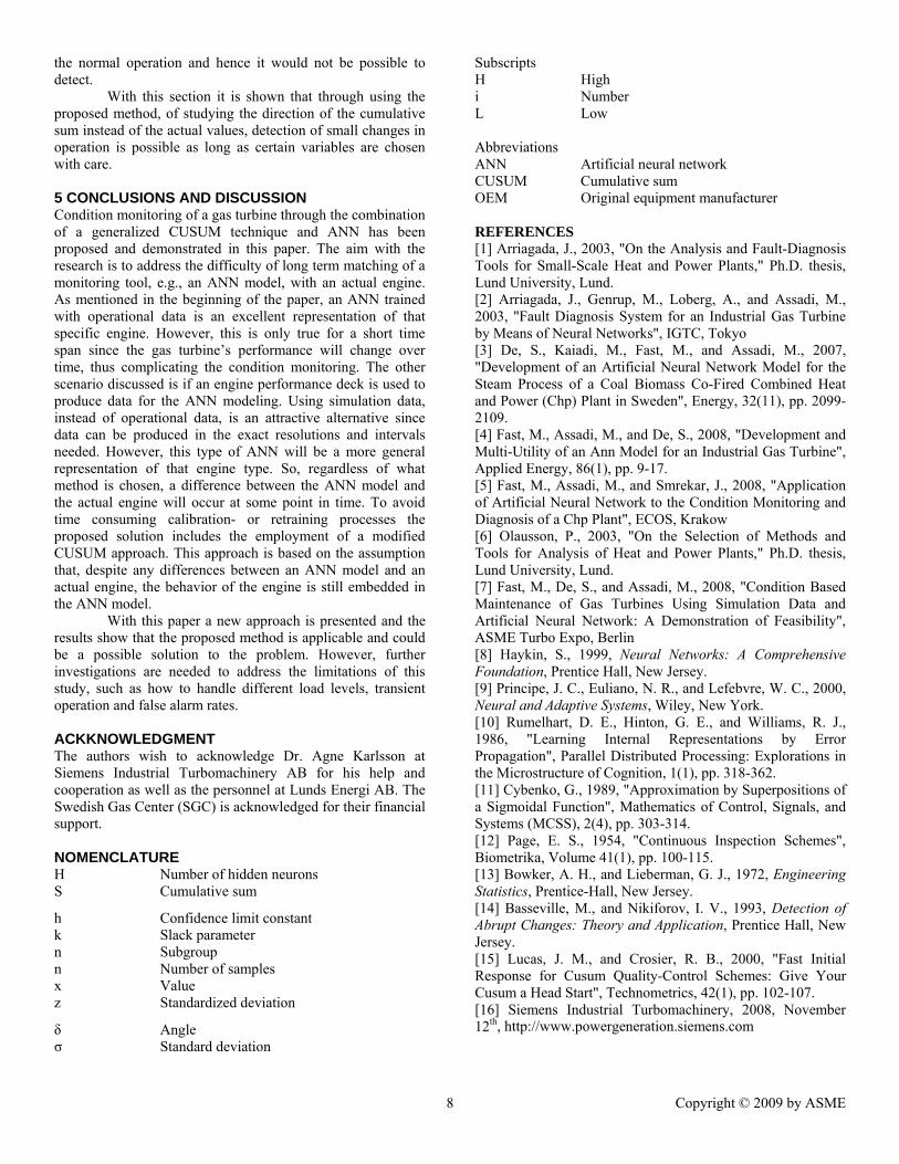
Copyright © 2009 by ASME 8

the normal operation and hence it would not be possible to detect.

With this section it is shown that through using the proposed method, of studying the direction of the cumulative sum instead of the actual values, detection of small changes in operation is possible as long as certain variables are chosen with care. 5 CONCLUSIONS AND DISCUSSION Condition monitoring of a gas turbine through the combination of a generalized CUSUM technique and ANN has been proposed and demonstrated in this paper. The aim with the research is to address the difficulty of long term matching of a monitoring tool, e.g., an ANN model, with an actual engine. As mentioned in the beginning of the paper, an ANN trained with operational data is an excellent representation of that specific engine. However, this is only true for a short time span since the gas turbine’s performance will change over time, thus complicating the condition monitoring. The other scenario discussed is if an engine performance deck is used to produce data for the ANN modeling. Using simulation data, instead of operational data, is an attractive alternative since data can be produced in the exact resolutions and intervals needed. However, this type of ANN will be a more general representation of that engine type. So, regardless of what method is chosen, a difference between the ANN model and the actual engine will occur at some point in time. To avoid time consuming calibration- or retraining processes the proposed solution includes the employment of a modified CUSUM approach. This approach is based on the assumption that, despite any differences between an ANN model and an actual engine, the behavior of the engine is still embedded in the ANN model. With this paper a new approach is presented and the results show that the proposed method is applicable and could be a possible solution to the problem. However, further investigations are needed to address the limitations of this study, such as how to handle different load levels, transient operation and false alarm rates. ACKKNOWLEDGMENT The authors wish to acknowledge Dr. Agne Karlsson at Siemens Industrial Turbomachinery AB for his help and cooperation as well as the personnel at Lunds Energi AB. The Swedish Gas Center (SGC) is acknowledged for their financial support. NOMENCLATURE H Number of hidden neurons S Cumulative sum

h Confidence limit constant k Slack parameter n Subgroup n Number of samples x Value z Standardized deviation

δ Angle σ Standard deviation

Subscripts H High i Number L Low Abbreviations ANN Artificial neural network CUSUM Cumulative sum OEM Original equipment manufacturer REFERENCES [1] Arriagada, J., 2003, "On the Analysis and Fault-Diagnosis Tools for Small-Scale Heat and Power Plants," Ph.D. thesis, Lund University, Lund. [2] Arriagada, J., Genrup, M., Loberg, A., and Assadi, M., 2003, "Fault Diagnosis System for an Industrial Gas Turbine by Means of Neural Networks", IGTC, Tokyo [3] De, S., Kaiadi, M., Fast, M., and Assadi, M., 2007, "Development of an Artificial Neural Network Model for the Steam Process of a Coal Biomass Co-Fired Combined Heat and Power (Chp) Plant in Sweden", Energy, 32(11), pp. 2099-2109. [4] Fast, M., Assadi, M., and De, S., 2008, "Development and Multi-Utility of an Ann Model for an Industrial Gas Turbine", Applied Energy, 86(1), pp. 9-17. [5] Fast, M., Assadi, M., and Smrekar, J., 2008, "Application of Artificial Neural Network to the Condition Monitoring and Diagnosis of a Chp Plant", ECOS, Krakow [6] Olausson, P., 2003, "On the Selection of Methods and Tools for Analysis of Heat and Power Plants," Ph.D. thesis, Lund University, Lund. [7] Fast, M., De, S., and Assadi, M., 2008, "Condition Based Maintenance of Gas Turbines Using Simulation Data and Artificial Neural Network: A Demonstration of Feasibility", ASME Turbo Expo, Berlin [8] Haykin, S., 1999, Neural Networks: A Comprehensive Foundation, Prentice Hall, New Jersey. [9] Principe, J. C., Euliano, N. R., and Lefebvre, W. C., 2000, Neural and Adaptive Systems, Wiley, New York. [10] Rumelhart, D. E., Hinton, G. E., and Williams, R. J., 1986, "Learning Internal Representations by Error Propagation", Parallel Distributed Processing: Explorations in the Microstructure of Cognition, 1(1), pp. 318-362. [11] Cybenko, G., 1989, "Approximation by Superpositions of a Sigmoidal Function", Mathematics of Control, Signals, and Systems (MCSS), 2(4), pp. 303-314. [12] Page, E. S., 1954, "Continuous Inspection Schemes", Biometrika, Volume 41(1), pp. 100-115. [13] Bowker, A. H., and Lieberman, G. J., 1972, Engineering Statistics, Prentice-Hall, New Jersey. [14] Basseville, M., and Nikiforov, I. V., 1993, Detection of Abrupt Changes: Theory and Application, Prentice Hall, New Jersey. [15] Lucas, J. M., and Crosier, R. B., 2000, "Fast Initial Response for Cusum Quality-Control Schemes: Give Your Cusum a Head Start", Technometrics, 42(1), pp. 102-107. [16] Siemens Industrial Turbomachinery, 2008, November 12th, http://www.powergeneration.siemens.com

Gas turbine sensor validation through classification with artificial neural networks

Fast M, Palmé T, Karlsson A. Presented at ECOS 2009, Foz do Iguaçu, Paraná, Brazil

Paper V

Proceedings of ECOS 2009 22nd International Conference on Efficiency, Cost, Optimization Copyright © 2009 by ABCM Simulation and Environmental Impact of Energy Systems August 31 – September 3, 2009, Foz do Iguaçu, Paraná, Brazil

GAS TURBINE SENSOR VALIDATION THROUGH CLASSIFICATION WITH ARTIFICIAL NEURAL NETWORKS

Magnus Fast, magnus.fast@energy.lth.se Division of Thermal Power Engineering, Department of Energy Sciences, Lund University, P.O. Box 118, S- 221 00 Lund, Sweden Thomas Palmé, thomas.palme@uis.no Department of Mechanical- and Structural Engineering and Materials Science, University of Stavanger, N-4036 Stavanger, Norway Agne Karlsson, agne.karlsson@siemens.com Siemens Industrial Turbomachinery AB, S-612 83 Finspång, Sweden Abstract. Modern power plants are all strongly dependent on reliable and accurate sensor readings for their monitoring and control, which makes the sensors an important part of any plant. Failing sensors can force a plant or component into non-optimal operation, failing sensors can also cause complete shut-downs of operation or in the worst case scenario cause damage to components. Due to their importance sensors need regular calibration and maintenance which is a time-consuming and therefore costly process. In this paper a method for evaluating sensor accuracy is presented with the goal of minimizing the need for calibration and at the same time avoiding shut-downs due to sensor faults etc. The proposed method consist of traning artificial neural networks as classifiers to recognize sensor drifts. The method is evaluated on two types of gas turbines, i.e., one single-shaft and one twin-shaft machine, and the results show early detection of sensor drifts for both types of machines as well as accurate production of soft measurements. Keywords: sensor validation, gas turbine, classification, artificial neural network

1. INTRODUCTION

The deregulation of the electricity market, and the consequent increase in competitiveness, drives the power producers to continuously investigate various means of keeping/increasing their profits. Improving the electrical efficiency through hardware upgrades is probably the most commonly employed measure, although the interest for improvements in plant utilization is on the rise. Improvement in plant utilization is often measured in reliability, availability and maintainability (RAM). Reliability and availability are measures of how many hours the plant operation can be uphold without unplanned or planned stops respectively. If one considers that the outage time is 3.6 days per percent reliability, then the need for efficient measures is clear. Especially, since many units of today have requirements of above 99 percent reliability. By improving the monitoring of a power plant or its components, there is a contingency of increasing the RAM. Improved monitoring could decrease the time spent on unplanned stops (i.e., increase the reliability) at the same time as maintenance could become more condition based instead of time based, which would extend the periods between overhauls (thereby increasing the availability).

Modern power plants are depending on accurate and reliable sensor readings for the control and monitoring of the plant and are therefore equipped with a considerable number of sensors. To avoid potential erroneous sensor signals affecting the operation of a plant, redundant sensors are often employed for crucial measurements. Sensors need regular maintenance and calibration, regardless of their condition, and the greater the number of sensors the more costly and time consuming this procedure becomes. Through employing some method of sensor validation, operational failures due to sensor faults can be avoided at the same time as sensor calibration can be based on sensor’s condition rather than schedules.

Sensor validation relies upon correlation between parameters and two common methods are principal component analysis (PCA) and partial least squares (PLS), both of which are linear methods, i.e., optimal when applied to linear systems. Another option is Kalman filters, which also are developed for linear systems but can be extended to cope with nonlinear systems. However, Kalman filters are model based (i.e., not data driven) and cannot be constructed with e.g., operational data. The success of Kalman filter models for sensor validation is therefore dependent on the fidelity of the system or component model. Artificial neural networks (ANNs) are one candidate which are able to tackle nonlinear systems as well as being developed from data without the need of model specifications (i.e., data driven). In 1991, Kramer proposed ANN for performing data compression by feature extraction without sacrificing the nonlinearity in the data (Kramer, 1991) and in Autoassociative neural network (Kramer, 1992), he extended his evaluation of the method and puts it into a sensor validation context and names it autoassociative neural network (AANN). This network is an identity mapper, containing three hidden layer layers with the following function in order: mapping, data compression and de-mapping. The actual implementation of an AANN for sensor validation is not straight forward and different approaches are suggested for the different sensor validation steps that are fault detection, isolation and accommodation (FDIA). One approach is to train the AANN with a healthy data set and subsequently evaluate the differences between inputs and outputs in order to detect a failing sensor. One problem with this method is that a failing sensor value is

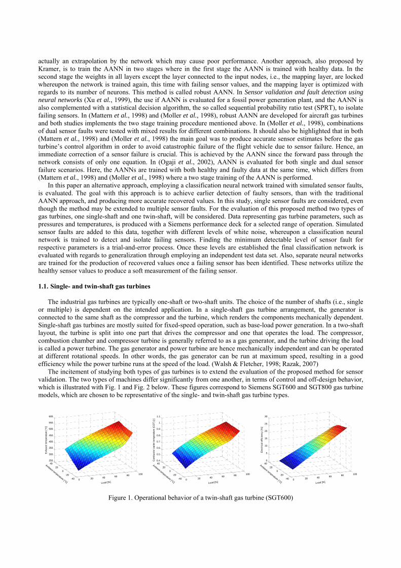
actually an extrapolation by the network which may cause poor performance. Another approach, also proposed by Kramer, is to train the AANN in two stages where in the first stage the AANN is trained with healthy data. In the second stage the weights in all layers except the layer connected to the input nodes, i.e., the mapping layer, are locked whereupon the network is trained again, this time with failing sensor values, and the mapping layer is optimized with regards to its number of neurons. This method is called robust AANN. In Sensor validation and fault detection using neural networks (Xu et al., 1999), the use if AANN is evaluated for a fossil power generation plant, and the AANN is also complemented with a statistical decision algorithm, the so called sequential probability ratio test (SPRT), to isolate failing sensors. In (Mattern et al., 1998) and (Moller et al., 1998), robust AANN are developed for aircraft gas turbines and both studies implements the two stage training procedure mentioned above. In (Moller et al., 1998), combinations of dual sensor faults were tested with mixed results for different combinations. It should also be highlighted that in both (Mattern et al., 1998) and (Moller et al., 1998) the main goal was to produce accurate sensor estimates before the gas turbine’s control algorithm in order to avoid catastrophic failure of the flight vehicle due to sensor failure. Hence, an immediate correction of a sensor failure is crucial. This is achieved by the AANN since the forward pass through the network consists of only one equation. In (Ogaji et al., 2002), AANN is evaluated for both single and dual sensor failure scenarios. Here, the AANNs are trained with both healthy and faulty data at the same time, which differs from (Mattern et al., 1998) and (Moller et al., 1998) where a two stage training of the AANN is performed.

In this paper an alternative approach, employing a classification neural network trained with simulated sensor faults, is evaluated. The goal with this approach is to achieve earlier detection of faulty sensors, than with the traditional AANN approach, and producing more accurate recovered values. In this study, single sensor faults are considered, even though the method may be extended to multiple sensor faults. For the evaluation of this proposed method two types of gas turbines, one single-shaft and one twin-shaft, will be considered. Data representing gas turbine parameters, such as pressures and temperatures, is produced with a Siemens performance deck for a selected range of operation. Simulated sensor faults are added to this data, together with different levels of white noise, whereupon a classification neural network is trained to detect and isolate failing sensors. Finding the minimum detectable level of sensor fault for respective parameters is a trial-and-error process. Once these levels are established the final classification network is evaluated with regards to generalization through employing an independent test data set. Also, separate neural networks are trained for the production of recovered values once a failing sensor has been identified. These networks utilize the healthy sensor values to produce a soft measurement of the failing sensor.

1.1. Single- and twin-shaft gas turbines

The industrial gas turbines are typically one-shaft or two-shaft units. The choice of the number of shafts (i.e., single

or multiple) is dependent on the intended application. In a single-shaft gas turbine arrangement, the generator is connected to the same shaft as the compressor and the turbine, which renders the components mechanically dependent. Single-shaft gas turbines are mostly suited for fixed-speed operation, such as base-load power generation. In a two-shaft layout, the turbine is split into one part that drives the compressor and one that operates the load. The compressor, combustion chamber and compressor turbine is generally referred to as a gas generator, and the turbine driving the load is called a power turbine. The gas generator and power turbine are hence mechanically independent and can be operated at different rotational speeds. In other words, the gas generator can be run at maximum speed, resulting in a good efficiency while the power turbine runs at the speed of the load. (Walsh & Fletcher, 1998; Razak, 2007)

The incitement of studying both types of gas turbines is to extend the evaluation of the proposed method for sensor validation. The two types of machines differ significantly from one another, in terms of control and off-design behavior, which is illustrated with Fig. 1 and Fig. 2 below. These figures correspond to Siemens SGT600 and SGT800 gas turbine models, which are chosen to be representative of the single- and twin-shaft gas turbine types.

0 20 40 60 80 100

-40-20

020

40250

300

350

400

450

500

550

600

Load [%]

Ambient temperature [°C]

Exh

aust

tem

pera

ture

[°C

]

0 20 40 60 80 100

-40-20

020

400.4

0.5

0.6

0.7

0.8

0.9

1

1.1

Load [%]

Ambient temperature [°C]

Com

bust

or o

utle

t tem

pera

ture

(CO

T) [-

]

0 20 40 60 80 100

-40-20

020

400

5

10

15

20

25

30

Load [%]

Ambient temperature [°C]

Ele

ctric

al e

ffici

ency

[%]

Figure 1. Operational behavior of a twin-shaft gas turbine (SGT600)

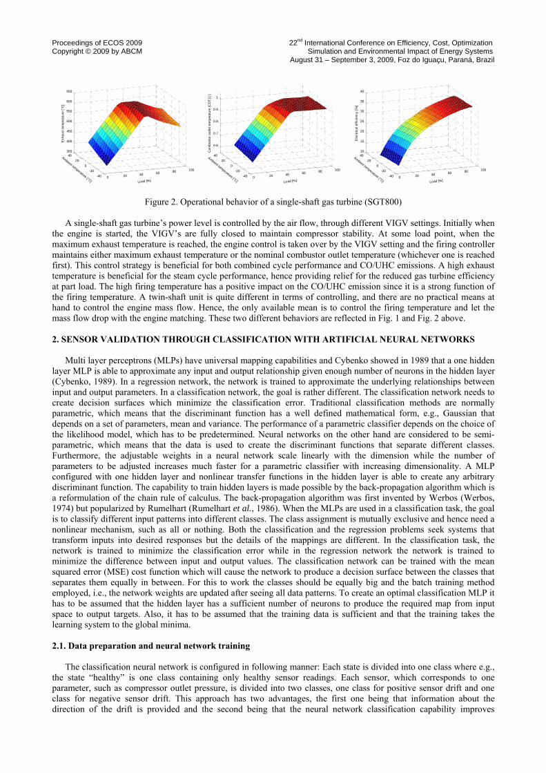
Proceedings of ECOS 2009 22nd International Conference on Efficiency, Cost, Optimization Copyright © 2009 by ABCM Simulation and Environmental Impact of Energy Systems August 31 – September 3, 2009, Foz do Iguaçu, Paraná, Brazil

0 20 40 60 80 100

-40-20

020

40350

400

450

500

550

600

650

Load [%]

Ambient temperature [°C]

Exh

aust

tem

pera

ture

[°C

]

0 20 40 60 80 100

-40-20

020

40

0.6

0.7

0.8

0.9

1

Load [%]

Ambient temperature [°C]

Com

bust

or o

utle

t tem

pera

ture

(CO

T) [-

]

0 20 40 60 80 100

-40-20

020

4010

15

20

25

30

35

40

Load [%]

Ambient temperature [°C]

Ele

ctric

al e

ffici

ency

[%]

Figure 2. Operational behavior of a single-shaft gas turbine (SGT800)

A single-shaft gas turbine’s power level is controlled by the air flow, through different VIGV settings. Initially when the engine is started, the VIGV’s are fully closed to maintain compressor stability. At some load point, when the maximum exhaust temperature is reached, the engine control is taken over by the VIGV setting and the firing controller maintains either maximum exhaust temperature or the nominal combustor outlet temperature (whichever one is reached first). This control strategy is beneficial for both combined cycle performance and CO/UHC emissions. A high exhaust temperature is beneficial for the steam cycle performance, hence providing relief for the reduced gas turbine efficiency at part load. The high firing temperature has a positive impact on the CO/UHC emission since it is a strong function of the firing temperature. A twin-shaft unit is quite different in terms of controlling, and there are no practical means at hand to control the engine mass flow. Hence, the only available mean is to control the firing temperature and let the mass flow drop with the engine matching. These two different behaviors are reflected in Fig. 1 and Fig. 2 above.

2. SENSOR VALIDATION THROUGH CLASSIFICATION WITH ARTIFICIAL NEURAL NETWORKS

Multi layer perceptrons (MLPs) have universal mapping capabilities and Cybenko showed in 1989 that a one hidden

layer MLP is able to approximate any input and output relationship given enough number of neurons in the hidden layer (Cybenko, 1989). In a regression network, the network is trained to approximate the underlying relationships between input and output parameters. In a classification network, the goal is rather different. The classification network needs to create decision surfaces which minimize the classification error. Traditional classification methods are normally parametric, which means that the discriminant function has a well defined mathematical form, e.g., Gaussian that depends on a set of parameters, mean and variance. The performance of a parametric classifier depends on the choice of the likelihood model, which has to be predetermined. Neural networks on the other hand are considered to be semi-parametric, which means that the data is used to create the discriminant functions that separate different classes. Furthermore, the adjustable weights in a neural network scale linearly with the dimension while the number of parameters to be adjusted increases much faster for a parametric classifier with increasing dimensionality. A MLP configured with one hidden layer and nonlinear transfer functions in the hidden layer is able to create any arbitrary discriminant function. The capability to train hidden layers is made possible by the back-propagation algorithm which is a reformulation of the chain rule of calculus. The back-propagation algorithm was first invented by Werbos (Werbos, 1974) but popularized by Rumelhart (Rumelhart et al., 1986). When the MLPs are used in a classification task, the goal is to classify different input patterns into different classes. The class assignment is mutually exclusive and hence need a nonlinear mechanism, such as all or nothing. Both the classification and the regression problems seek systems that transform inputs into desired responses but the details of the mappings are different. In the classification task, the network is trained to minimize the classification error while in the regression network the network is trained to minimize the difference between input and output values. The classification network can be trained with the mean squared error (MSE) cost function which will cause the network to produce a decision surface between the classes that separates them equally in between. For this to work the classes should be equally big and the batch training method employed, i.e., the network weights are updated after seeing all data patterns. To create an optimal classification MLP it has to be assumed that the hidden layer has a sufficient number of neurons to produce the required map from input space to output targets. Also, it has to be assumed that the training data is sufficient and that the training takes the learning system to the global minima. 2.1. Data preparation and neural network training

The classification neural network is configured in following manner: Each state is divided into one class where e.g.,

the state “healthy” is one class containing only healthy sensor readings. Each sensor, which corresponds to one parameter, such as compressor outlet pressure, is divided into two classes, one class for positive sensor drift and one class for negative sensor drift. This approach has two advantages, the first one being that information about the direction of the drift is provided and the second being that the neural network classification capability improves

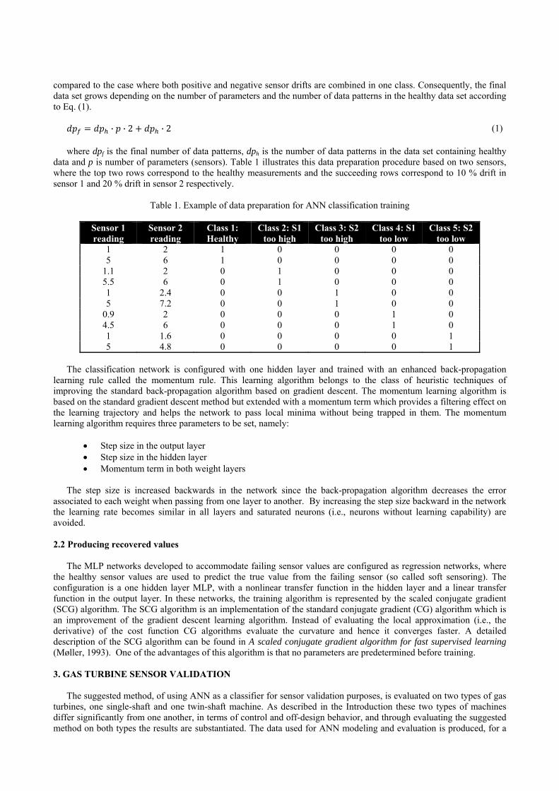
compared to the case where both positive and negative sensor drifts are combined in one class. Consequently, the final data set grows depending on the number of parameters and the number of data patterns in the healthy data set according to E (1q. ).

· · 2 · 2 (1)

where dpf is the final number of data patterns, dph is the number of data patterns in the data set containing healthy

data and p is number of parameters (sensors). Table 1 illustrates this data preparation procedure based on two sensors, where the top two rows correspond to the healthy measurements and the succeeding rows correspond to 10 % drift in sensor 1 and 20 % drift in sensor 2 respectively.

Table 1. Example of data preparation for ANN classification training

Sensor 1 reading

Sensor 2 reading

Class 1: Healthy

Class 2: S1 too high

Class 3: S2 too high

Class 4: S1 too low

Class 5: S2 too low

1 2 1 0 0 0 0 5 6 1 0 0 0 0

1.1 2 0 1 0 0 0 5.5 6 0 1 0 0 0 1 2.4 0 0 1 0 0 5 7.2 0 0 1 0 0

0.9 2 0 0 0 1 0 4.5 6 0 0 0 1 0 1 1.6 0 0 0 0 1 5 4.8 0 0 0 0 1

The classification network is configured with one hidden layer and trained with an enhanced back-propagation

learning rule called the momentum rule. This learning algorithm belongs to the class of heuristic techniques of improving the standard back-propagation algorithm based on gradient descent. The momentum learning algorithm is based on the standard gradient descent method but extended with a momentum term which provides a filtering effect on the learning trajectory and helps the network to pass local minima without being trapped in them. The momentum learning algorithm requires three parameters to be set, namely:

• Step size in the output layer • Step size in the hidden layer • Momentum term in both weight layers

The step size is increased backwards in the network since the back-propagation algorithm decreases the error

associated to each weight when passing from one layer to another. By increasing the step size backward in the network the learning rate becomes similar in all layers and saturated neurons (i.e., neurons without learning capability) are avoided.

2.2 Producing recovered values

The MLP networks developed to accommodate failing sensor values are configured as regression networks, where

the healthy sensor values are used to predict the true value from the failing sensor (so called soft sensoring). The configuration is a one hidden layer MLP, with a nonlinear transfer function in the hidden layer and a linear transfer function in the output layer. In these networks, the training algorithm is represented by the scaled conjugate gradient (SCG) algorithm. The SCG algorithm is an implementation of the standard conjugate gradient (CG) algorithm which is an improvement of the gradient descent learning algorithm. Instead of evaluating the local approximation (i.e., the derivative) of the cost function CG algorithms evaluate the curvature and hence it converges faster. A detailed description of the SCG algorithm can be found in A scaled conjugate gradient algorithm for fast supervised learning (Møller, 1993). One of the advantages of this algorithm is that no parameters are predetermined before training. 3. GAS TURBINE SENSOR VALIDATION

The suggested method, of using ANN as a classifier for sensor validation purposes, is evaluated on two types of gas turbines, one single-shaft and one twin-shaft machine. As described in the Introduction these two types of machines differ significantly from one another, in terms of control and off-design behavior, and through evaluating the suggested method on both types the results are substantiated. The data used for ANN modeling and evaluation is produced, for a

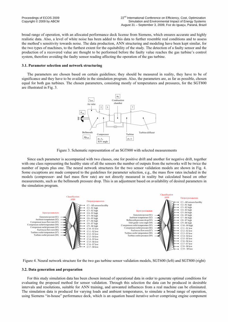
Proceedings of ECOS 2009 22nd International Conference on Efficiency, Cost, Optimization Copyright © 2009 by ABCM Simulation and Environmental Impact of Energy Systems August 31 – September 3, 2009, Foz do Iguaçu, Paraná, Brazil

broad range of operation, with an allocated performance deck license from Siemens, which ensures accurate and highly realistic data. Also, a level of white noise has been added to this data to further resemble real conditions and to assess the method’s sensitivity towards noise. The data production, ANN structuring and modeling have been kept similar, for the two types of machines, to the furthest extent for the equitability of the study. The detection of a faulty sensor and the production of a recovered value are thought to be performed before the faulty value reaches the gas turbine’s control system, therefore avoiding the faulty sensor reading affecting the operation of the gas turbine.

3.1. Parameter selection and network structuring

The parameters are chosen based on certain guidelines; they should be measured in reality, they have to be of

significance and they have to be available in the simulation program. Also, the parameters are, as far as possible, chosen equal for both gas turbines. The chosen parameters, consisting mostly of temperatures and pressures, for the SGT800 are illustrated in Fig. 3.

tamb

p3, t3,IGV angle

p7, t7

BellmouthCompressor

Combustionchamber

TurbineTurbine diffuser

mf

Pout

2 3 7

dpbell

Air inlet

Figure 3. Schematic representation of an SGT800 with selected measurements

Since each parameter is accompanied with two classes, one for positive drift and another for negative drift, together

with one class representing the healthy state of all the sensors the number of outputs from the networks will be twice the number of inputs plus one. The neural network structures for the two sensor validation models are shown in Fig. 4. Some exceptions are made compared to the guidelines for parameter selection, e.g., the mass flow rates included in the models (compressor- and fuel mass flow rate) are not directly measured in reality but calculated based on other measurements, such as the bellmouth pressure drop. This is an adjustment based on availability of desired parameters in the simulation program.

Figure 4. Neural network structure for the two gas turbine sensor validation models, SGT600 (left) and SGT800 (right)

3.2. Data generation and preparation For this study simulation data has been chosen instead of operational data in order to generate optimal conditions for

evaluating the proposed method for sensor validation. Through this selection the data can be produced in desirable intervals and resolutions, suitable for ANN training, and unwanted influences from a real machine can be eliminated. The simulation data is produced for varying loads and ambient temperatures, to simulate a broad range of operation, using Siemens “in-house” performance deck, which is an equation based iterative solver comprising engine component

. . .. . .

Generator power (S1)Ambient temperature (S2)

Compressor mass flow rate (S3)Compressor outlet temperature (S4)

Compressor outlet pressure (S5)Fuel mass flow rate (S6)

Turbine outlet temperature (S7)Turbine outlet pressure (S8)

Input parameters

Output parameters

Classification ANN

. . .. . .

Generator power (S1)Ambient temperature (S2)

Bellmouth pressure drop (S3)Inlet guide vane angle (S4)

Compressor outlet temperature (S5)Compressor outlet pressure (S6)

Fuel mass flow rate (S7)Turbine outlet temperature (S8)

Turbine outlet pressure (S9)

Input parameters

Output parametersClassification

ANN

C1 - All sensors healthyC2 - S1 highC3 - S2 highC4 - S3 highC5 - S4 highC6 - S5 highC7 - S6 highC8 - S7 highC9 - S8 highC10 - S9 highC11 - S1 lowC12 - S2 lowC13 - S3 lowC14 - S4 lowC15 - S5 lowC16 - S6 lowC17 - S7 lowC18 - S8 lowC19 – S9 low

C1 - All sensors healthyC2 - S1 highC3 - S2 highC4 - S3 highC5 - S4 highC6 - S5 highC7 - S6 highC8 - S7 highC9 - S8 highC10 - S1 lowC11 - S2 lowC12 - S3 lowC13 - S4 lowC14 - S5 lowC15 - S6 lowC16 - S7 lowC17 - S8 low

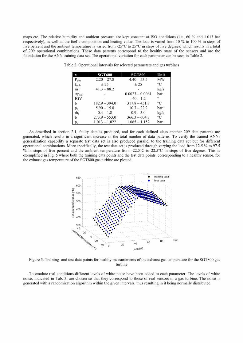
maps etc. The relative humidity and ambient pressure are kept constant at ISO conditions (i.e., 60 % and 1.013 bar respectively), as well as the fuel’s composition and heating value. The load is varied from 10 % to 100 % in steps of five percent and the ambient temperature is varied from -25°C to 25°C in steps of five degrees, which results in a total of 209 operational combinations. These data patterns correspond to the healthy state of the sensors and are the foundation for the ANN training data set. The operational variation for each parameter can be seen in Table 2.

Table 2. Operational intervals for selected parameters and gas turbines

x SGT600 SGT800 Unit Pgen

2.20 – 27.8 4.40 – 53.5 MW tamb

± 25 ± 25 °C ṁc 41.3 – 88.2 - kg/s ∆pbell - 0.0023 – 0.0061 bar IGV - -40 – 1.2 ° t3 182.9 – 394.0 317.8 – 451.8 °C p3 5.90 – 15.8 10.7 – 22.2 bar ṁf 0.4 – 1.8 0.9 – 3.0 kg/s t7 273.9 – 553.0 366.3 – 604.7 °C p7 1.013 – 1.022 1.065 – 1.152 bar

As described in section 2.1, faulty data is produced, and for each defined class another 209 data patterns are

generated, which results in a significant increase in the total number of data patterns. To verify the trained ANNs generalization capability a separate test data set is also produced parallel to the training data set but for different operational combinations. More specifically, the test data set is produced through varying the load from 12.5 % to 97.5 % in steps of five percent and the ambient temperature from -22.5°C to 22.5°C in steps of five degrees. This is exemplified in Fig. 5 where both the training data points and the test data points, corresponding to a healthy sensor, for the exhaust gas temperature of the SGT800 gas turbine are plotted.

0 20 40 60 80 100

-40-20

020

40350

400

450

500

550

600

650

Load [%]

Ambient temperature [°C]

Exh

aust

tem

pera

ture

[°C

]

Training dataTest data

Figure 5. Training- and test data points for healthy measurements of the exhaust gas temperature for the SGT800 gas turbine

To emulate real conditions different levels of white noise have been added to each parameter. The levels of white

noise, indicated in Tab. 3, are chosen so that they correspond to those of real sensors in a gas turbine. The noise is generated with a randomization algorithm within the given intervals, thus resulting in it being normally distributed.

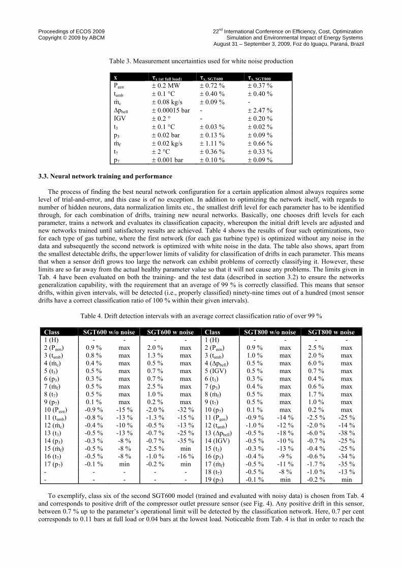
Proceedings of ECOS 2009 22nd International Conference on Efficiency, Cost, Optimization Copyright © 2009 by ABCM Simulation and Environmental Impact of Energy Systems August 31 – September 3, 2009, Foz do Iguaçu, Paraná, Brazil

Table 3. Measurement uncertainties used for white noise production

x τx (at full load) τx, SGT600 τx, SGT800 Pgen ± 0.2 MW ± 0.72 % ± 0.37 % tamb ± 0.1 °C ± 0.40 % ± 0.40 % ṁc ± 0.08 kg/s ± 0.09 % - ∆pbell

± 0.00015 bar - ± 2.47 % IGV ± 0.2 ° - ± 0.20 % t3 ± 0.1 °C ± 0.03 % ± 0.02 % p3 ± 0.02 bar ± 0.13 % ± 0.09 % ṁf ± 0.02 kg/s ± 1.11 % ± 0.66 % t7 ± 2 °C ± 0.36 % ± 0.33 % p7 ± 0.001 bar ± 0.10 % ± 0.09 %

3.3. Neural network training and performance

The process of finding the best neural network configuration for a certain application almost always requires some

level of trial-and-error, and this case is of no exception. In addition to optimizing the network itself, with regards to number of hidden neurons, data normalization limits etc., the smallest drift level for each parameter has to be identified through, for each combination of drifts, training new neural networks. Basically, one chooses drift levels for each parameter, trains a network and evaluates its classification capacity, whereupon the initial drift levels are adjusted and new networks trained until satisfactory results are achieved. Table 4 shows the results of four such optimizations, two for each type of gas turbine, where the first network (for each gas turbine type) is optimized without any noise in the data and subsequently the second network is optimized with white noise in the data. The table also shows, apart from the smallest detectable drifts, the upper/lower limits of validity for classification of drifts in each parameter. This means that when a sensor drift grows too large the network can exhibit problems of correctly classifying it. However, these limits are so far away from the actual healthy parameter value so that it will not cause any problems. The limits given in Tab. 4 have been evaluated on both the training- and the test data (described in section 3.2) to ensure the networks generalization capability, with the requirement that an average of 99 % is correctly classified. This means that sensor drifts, within given intervals, will be detected (i.e., properly classified) ninety-nine times out of a hundred (most sensor drifts have a correct classification ratio of 100 % within their given intervals).

Table 4. Drift detection intervals with an average correct classification ratio of over 99 %

Class SGT600 w/o noise SGT600 w noise Class SGT800 w/o noise SGT800 w noise 1 (H) - - - - 1 (H) - - - - 2 (Pgen) 0.9 % max 2.0 % max 2 (Pgen) 0.9 % max 2.5 % max 3 (tamb) 0.8 % max 1.3 % max 3 (tamb) 1.0 % max 2.0 % max 4 (ṁc) 0.4 % max 0.5 % max 4 (∆pbell) 0.5 % max 6.0 % max 5 (t3) 0.5 % max 0.7 % max 5 (IGV) 0.5 % max 0.7 % max 6 (p3) 0.3 % max 0.7 % max 6 (t3) 0.3 % max 0.4 % max 7 (ṁf) 0.5 % max 2.5 % max 7 (p3) 0.4 % max 0.6 % max 8 (t7) 0.5 % max 1.0 % max 8 (ṁf) 0.5 % max 1.7 % max 9 (p7) 0.1 % max 0.2 % max 9 (t7) 0.5 % max 1.0 % max 10 (Pgen) -0.9 % -15 % -2.0 % -32 % 10 (p7) 0.1 % max 0.2 % max 11 (tamb) -0.8 % -13 % -1.3 % -15 % 11 (Pgen) -0.9 % -14 % -2.5 % -25 % 12 (ṁc) -0.4 % -10 % -0.5 % -13 % 12 (tamb) -1.0 % -12 % -2.0 % -14 % 13 (t3) -0.5 % -13 % -0.7 % -25 % 13 (∆pbell) -0.5 % -18 % -6.0 % -38 % 14 (p3) -0.3 % -8 % -0.7 % -35 % 14 (IGV) -0.5 % -10 % -0.7 % -25 % 15 (ṁf) -0.5 % -8 % -2.5 % min 15 (t3) -0.3 % -13 % -0.4 % -25 % 16 (t7) -0.5 % -8 % -1.0 % -16 % 16 (p3) -0.4 % -9 % -0.6 % -34 % 17 (p7) -0.1 % min -0.2 % min 17 (ṁf) -0.5 % -11 % -1.7 % -35 % - - - - - 18 (t7) -0.5 % -8 % -1.0 % -13 % - - - - - 19 (p7) -0.1 % min -0.2 % min

To exemplify, class six of the second SGT600 model (trained and evaluated with noisy data) is chosen from Tab. 4

and corresponds to positive drift of the compressor outlet pressure sensor (see Fig. 4). Any positive drift in this sensor, between 0.7 % up to the parameter’s operational limit will be detected by the classification network. Here, 0.7 per cent corresponds to 0.11 bars at full load or 0.04 bars at the lowest load. Noticeable from Tab. 4 is that in order to reach the

same correct classification ratio when training with noisy data the drift levels for training has to be increased somewhat. On the other hand, this has a positive side-effect as well since the ANNs trained with slightly higher drift levels have wider drift detection intervals. Another aspect noticeable from Tab. 4 is that all positive sensor drifts are classified correctly within the entire operational range while the majority of the negative sensor drifts have slightly more narrow drift detection intervals.

Since the simulation data is produced by varying two parameters, load and ambient temperature, it is possible to illustrate the classes as regions in a three dimensional space and thereby visualizing the accuracy of the evaluated classification method. An example is made using the exhaust gas temperature of the SGT600 gas turbine and plotting classes eight (positive drift) and sixteen (negative drift), shown in Fig. 6. Actual parameter values, drift levels and intervals are displayed in the figure.

Figure 6. Representation of two classes in a three dimensional space for positive and negative drift of an SGT600 exhaust gas temperature sensor

As long as the parameter value (i.e., the exhaust gas temperature measurement) remains in between the two classes,

represented by the regions in Fig. 6, the sensor is deemed as healthy. Once the parameter value crosses into one of these regions it will be classified as drifting, positive drift for the upper region and negative drift for the lower region. Positive sensor drift can be detected in the entire operational range, as for all parameters, while negative drift has a lower limitation at 16 % of the correct value. However, this lower level is large enough to be fully detectable with conventional methods, such as logical expressions. 3.4 Producing recovered values

Once a failing sensor has been identified by a classification neural network a recovered value can be reproduced through using the remaining, healthy sensors. This is achieved through employing individual regression neural networks, using the healthy sensors as inputs and the desired parameter as output, which is an easy and reliable way of producing accurate recovered values. Table 5 shows the prediction accuracy of the ANN soft sensoring models where the average error is calculated through using the predictions from the ANN models, which is trained with noisy data, and comparing it with corresponding values without the noise (i.e., the actual parameter values). A closer look at Tab. 5 reveals that most of the sensor values are reproduced below the given levels of white noise, indicating that the noise is “filtered” out during the training of the networks. This also means that the ANN predictions are at least as good as those of a healthy sensor.

Proceedings of ECOS 2009 22nd International Conference on Efficiency, Cost, Optimization Copyright © 2009 by ABCM Simulation and Environmental Impact of Energy Systems August 31 – September 3, 2009, Foz do Iguaçu, Paraná, Brazil

Table 5. Average error for prediction of soft measurements

x SGT600 SGT800 tamb

0.03 % 0.23 % Pgen

0.24 % 0.33 % ṁc 0.07 % - ∆pbell - 0.39 % IGV - 0.11 % t3 0.08 % 0.08 % p3 0.07 % 0.07 % ṁf 0.35 % 0.23 % t7 0.10 % 0.23 % p7 0.02 % 0.03 %

4. SUMMARY AND DISCUSSION

This study has demonstrated a complete solution for sensor fault detection, isolation and accommodation through

employing ANN as a classifier in combination with ANNs configured as a regression networks for the production of soft measurements. An important advantage to highlight is that the algorithm can be developed with operational data without the need of a detailed model of the system. The method has been tested on two types of gas turbines, one single-shaft machine and one twin-shaft machine, and good results, in terms of detection of small sensor drifts as well as production of accurate soft measurements, have been achieved in both cases. By evaluating two different gas turbine types the method’s generic capability is highlighted. However, the method is applicable not only on the specific machines evaluated in this study but on all types of systems and components where sensors have some type of internal correlation. In this study single sensor faults have been tested and one natural extension of this study would be to evaluate multiple sensor faults. Other interesting extensions of this study would be to assess the influence of component degradation, and combining the method with a sequential analysis technique, such as cumulative sum (CUSUM), to achieve even earlier drift detection through studying sequences of data.

As often when dealing with data driven methods and neural networks there is a lot of trial-and-error work involved, which makes it impossible to exactly state what can be expected when applying this method. Detection of sensor faults depends on many factors, such as the amount of data used for training, what resolution it has and in what operational range it is available, the levels of noise in the data, the number of parameters considered etc. One of the main issues with this method is to select a well representative data set representing the healthy state, since the final data set grows substantially which results in long training periods when considering optimization of e.g., the number of neurons in the hidden layer. ACKNOWLEDGEMENTS

The authors of this paper greatly acknowledge Siemens Industrial Turbomachinery AB for providing the necessary tools for this study as well as assisting with technical support. The authors also express their gratitude towards the Swedish Gas Center AB (SGC) for their financial support. NOMENCLATURE C Class H Healthy P Power S Sensor dp Pressure difference, also data pattern m Mass flow rate p Pressure, also parameter t Temperature x Parameter Greek τ Noise level Subscripts 3 Compressor outlet

7 Turbine outlet amb Ambient bell Bellmouth c Compressor f Fuel, also final gen Generator h Healthy

Abbreviations AANN Auto-associative neural network ANN Artificial neural network CG Conjugate gradient CO Carbon monoxide COT Combustor outlet temperature CUSUM Cumulative sum FDIA Fault detection, isolation and accommodation

MLP Multi layer perceptron MSE Mean squared error PCA Partial component analysis PLS Partial least squares RAM Reliability, availability and

maintainability

SCG Scaled conjugate gradient SGT Siemens gas turbine UHC Unburned hydrocarbons (V)IGV (Variable) inlet guide vanes

REFERENCES Cybenko, G., 1989, "Approximation by superpositions of a sigmoidal function". Mathematics of Control, Signals, and

Systems (MCSS), Vol.2, No.4, pp.303-314. Kramer, M. A., 1991, "Nonlinear principal component analysis using autoassociative neural networks". AIChE journal,

Vol.37, No.2, pp.233-243. Kramer, M. A., 1992, "Autoassociative neural networks". Computers in Chemical Engineering, Vol.16, No.4, pp.313-

328. Mattern, D. L., Law, L. C., Guo, T. H., 1998, "Using neural networks for sensor validation", 34th Joint Propulsion

Conference, AIAA-98-3542. Moller, J. C., Litt, J. S., Guo, T. H., 1998, "Neural network-based sensor validation for turboshaft engines", 34th Joint

Propulsion Conference, AIAA-98-3605. Møller, M. F., 1993, "A scaled conjugate gradient algorithm for fast supervised learning". Neural Networks, Vol.6,

pp.525-533. Ogaji, S. O. T., Singh, R., Probert, S. D., 2002, "Multiple-sensor fault-diagnoses for a 2-shaft stationary gas-turbine".

Applied energy, Vol.71, No.4, pp.321-339. Razak, A. M. Y., 2007, "Industrial Gas Turbines: Performance & Operability", Cambridge: Woodhead Publishing

Limited. Rumelhart, D. E., Hinton, G. E., Williams, R. J., 1986, "Learning internal representations by error propagation". Parallel

distributed processing, Vol.1, pp.318-62. Walsh, P. P., Fletcher, P., 1998, "Gas Turbine Performance", Oxford: Blackwell Science. Werbos, P. J., 1974, "Beyond regression: New tools for prediction and analysis in the behavioral sciences": Harvard

University. Xu, X., Hines, J. W., Uhrig, R. E., 1999, "Sensor validation and fault detection using neural networks", Maintenance

and Reliability Center, The University of Tenessee, Knoxville. RESPONSIBILITY NOTICE

The authors are the only responsible for the printed material included in this paper.