Embed Size (px)
Citation preview

CS 561, Session 28 1
Artificial Neural Networks and AI
Artificial Neural Networks provide…
- A new computing paradigm
- A technique for developing trainable classifiers, memories, dimension-reducing mappings, etc
- A tool to study brain function
CS 561, Session 28 2
Converging Frameworks
• Artificial intelligence (AI): build a “packet of intelligence” into a machine
• Cognitive psychology: explain human behavior by interacting processes (schemas) “in the head” but not localized in the brain
• Brain Theory: interactions of components of the brain -
- computational neuroscience - neurologically constrained-models
• and abstracting from them as both Artificial intelligence andCognitive psychology:- connectionism: networks of trainable “quasi-neurons” to provide “parallel distributed models” little constrained by neurophysiology- abstract (computer program or control system) information processing models

CS 561, Session 28 3
Vision, AI and ANNs
• 1940s: beginning of Artificial Neural Networks
McCullogh & Pitts, 1942Σi wixi ≥ θ
Perceptron learning rule (Rosenblatt, 1962)BackpropagationHopfield networks (1982)Kohonen self-organizing maps…
input outputneuron
m MSm
CS 561, Session 28 4
Vision, AI and ANNs
1950s: beginning of computer visionAim: give to machines same or better vision capability as oursDrive: AI, robotics applications and factory automation
Initially: passive, feedforward, layered and hierarchical processthat was just going to provide input to higher reasoningprocesses (from AI)
But soon: realized that could not handle real images
1980s: Active vision: make the system more robust by allowing thevision to adapt with the ongoing recognition/interpretation

CS 561, Session 28 5

CS 561, Session 28 6

CS 561, Session 28 7
Major Functional Areas
• Primary motor: voluntary movement• Primary somatosensory: tactile, pain, pressure, position, temp., mvt.• Motor association: coordination of complex movements• Sensory association: processing of multisensorial information• Prefrontal: planning, emotion, judgement• Speech center (Broca’s area): speech production and articulation• Wernicke’s area: comprehen-• sion of speech• Auditory: hearing• Auditory association: complex• auditory processing• Visual: low-level vision• Visual association: higher-level• vision
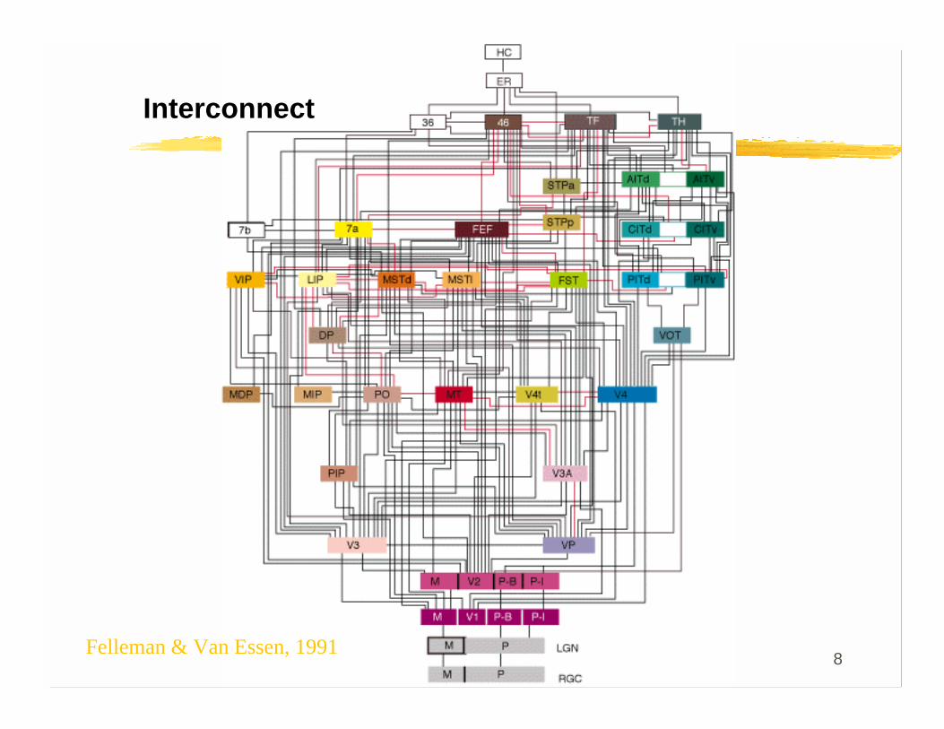
CS 561, Session 28 8Felleman & Van Essen, 1991
Interconnect

CS 561, Session 28 9
More on Connectivity
CS 561, Session 28 10
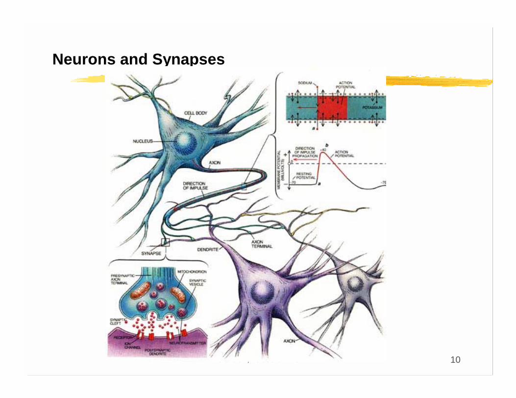
Neurons and Synapses

CS 561, Session 28 11
Electron Micrograph of a Real Neuron

CS 561, Session 28 12
Transmenbrane Ionic Transport
• Ion channels act as gates that allow or block the flow of specific ions into and out of the cell.

CS 561, Session 28 13
The Cable Equation
• See http://diwww.epfl.ch/~gerstner/SPNM/SPNM.htmlfor excellent additional material (some reproduced here).
• Just a piece of passive dendrite can yield complicated differential equations which have been extensively studied by electronicians in the context of the study of coaxial cables (TV antenna cable):

CS 561, Session 28 14
The Hodgkin-Huxley Model
Example spike trains obtained…

CS 561, Session 28 15
Detailed Neural Modeling
• A simulator, called “Neuron” has been developedat Yale to simulate the Hodgkin-Huxley equations,as well as other membranes/channels/etc.See http://www.neuron.yale.edu/

CS 561, Session 28 16
The "basic" biological neuron
• The soma and dendrites act as the input surface; the axon carries the outputs.
• The tips of the branches of the axon form synapses upon other neurons or upon effectors (though synapses may occur along the branches of an axon as well as the ends). The arrows indicate the direction of "typical" information flow from inputs to outputs.
Dendrites Soma Axon with branches andsynaptic terminals
CS 561, Session 28 17
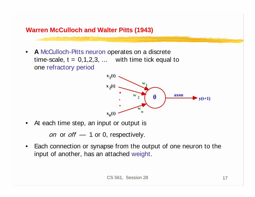
• A McCulloch-Pitts neuron operates on a discrete time-scale, t = 0,1,2,3, ... with time tick equal to one refractory period
• At each time step, an input or output is
on or off — 1 or 0, respectively.
• Each connection or synapse from the output of one neuron to the input of another, has an attached weight.
Warren McCulloch and Walter Pitts (1943)
x (t)1
x (t)n
x (t)2
y(t+1)
w1
2
n
w
w
axonθθθθ

CS 561, Session 28 18
Excitatory and Inhibitory Synapses
• We call a synapse
excitatory if wi > 0, and
inhibitory if wi < 0.
• We also associate a threshold θ with each neuron
• A neuron fires (i.e., has value 1 on its output line) at time t+1 if the weighted sum of inputs at t reaches or passes θ:
y(t+1) = 1 if and only if ΣΣΣΣ wixi(t) ≥≥≥≥ θθθθ
CS 561, Session 28 19
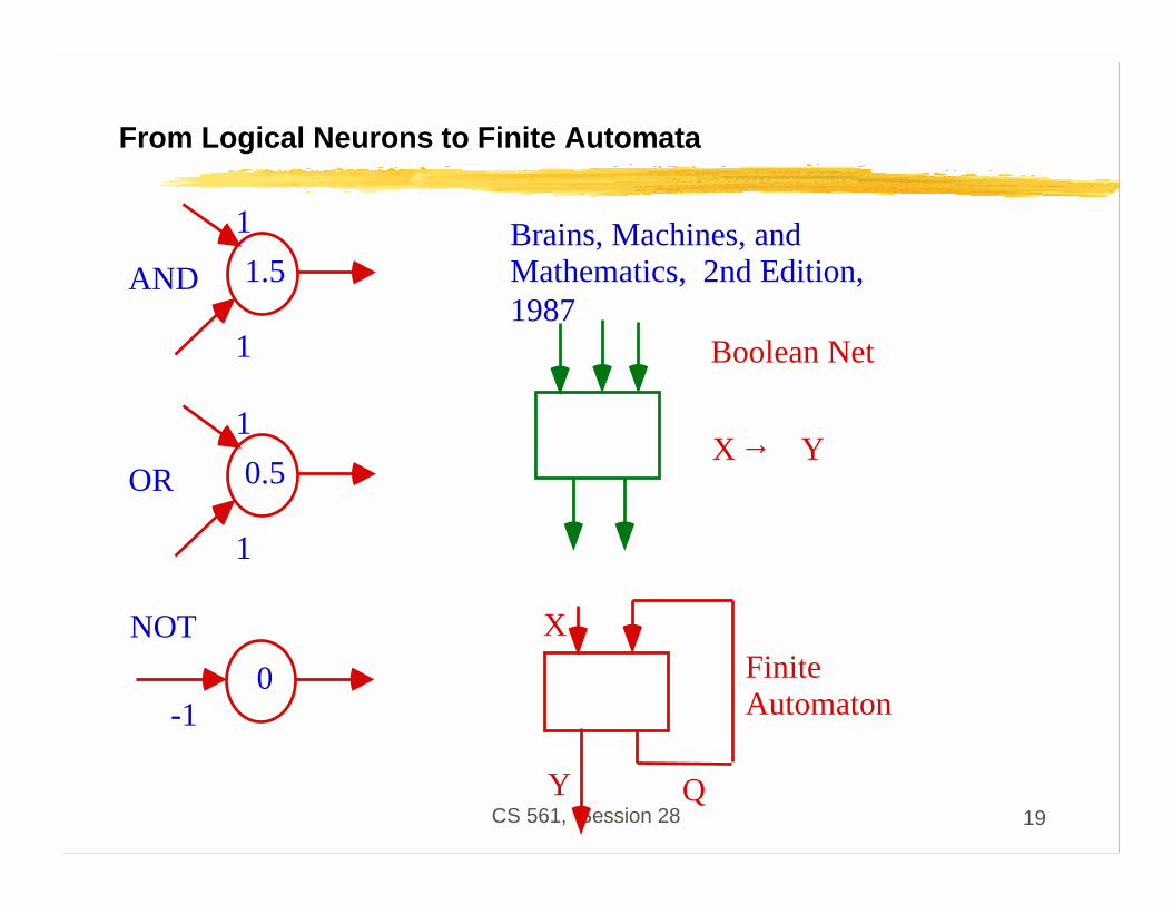
From Logical Neurons to Finite Automata
AND
1
1
1.5
NOT
-10
OR
1
1
0.5
Brains, Machines, and Mathematics, 2nd Edition, 1987
X Y→
Boolean Net
X
Y Q
Finite Automaton

CS 561, Session 28 20
Increasing the Realism of Neuron Models
• The McCulloch-Pitts neuron of 1943 is important
as a basis for
• logical analysis of the neurally computable, and
• current design of some neural devices (especially when augmented by learning rules to adjust synaptic weights).
• However, it is no longer considered a useful model for making contact with neurophysiological data concerning real neurons.
CS 561, Session 28 21
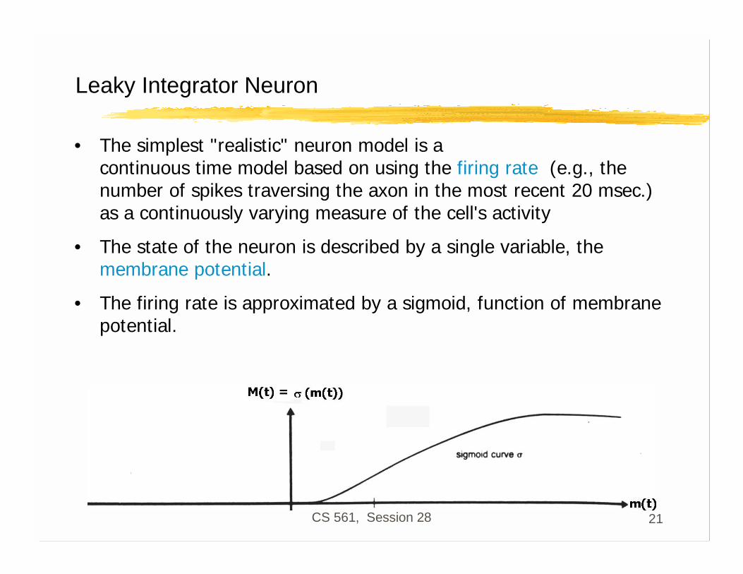
Leaky Integrator Neuron
• The simplest "realistic" neuron model is a continuous time model based on using the firing rate (e.g., the number of spikes traversing the axon in the most recent 20 msec.) as a continuously varying measure of the cell's activity
• The state of the neuron is described by a single variable, the membrane potential.
• The firing rate is approximated by a sigmoid, function of membrane potential.
CS 561, Session 28 22
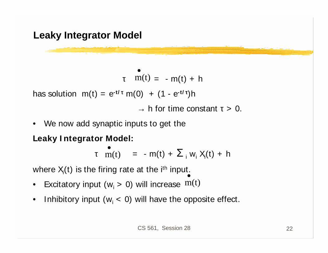
Leaky Integrator Model
τ = - m(t) + h
has solution m(t) = e-t/ττττ m(0) + (1 - e-t/ττττ)h
→ h for time constant τ > 0.
• We now add synaptic inputs to get the
Leaky Integrator Model:
τ = - m(t) + Σ i wi Xi(t) + h
where Xi(t) is the firing rate at the ith input.
• Excitatory input (wi > 0) will increase
• Inhibitory input (wi < 0) will have the opposite effect.
m(t)
m(t)
m(t)

CS 561, Session 28 23
Hopfield Networks
• A paper by John Hopfield in 1982 was the catalyst in attracting the attention of many physicists to "Neural Networks".
• In a network of McCulloch-Pitts neuronswhose output is 1 iff Σwij sj ≥ θi and is otherwise 0,neurons are updated synchronously: every neuron processes its inputs at each time step to determine a new output.

CS 561, Session 28 24
Hopfield Networks
• A Hopfield net (Hopfield 1982) is a net of such units subject to the asynchronous rule for updating one neuron at a time:
"Pick a unit i at random. If Σwij sj ≥ θi, turn it on. Otherwise turn it off."
• Moreover, Hopfield assumes symmetric weights:wij = wji

CS 561, Session 28 25
“Energy” of a Neural Network
• Hopfield defined the “energy”:
E = - ½ Σ ij sisjwij + Σ i siθi
• If we pick unit i and the firing rule (previous slide) does not change its si, it will not change E.

CS 561, Session 28 26
si: 0 to 1 transition
• If si initially equals 0, and Σ wijsj ≥ θi
then si goes from 0 to 1 with all other sj constant, and the "energy gap", or change in E, is given by
∆E = - ½ Σj (wijsj + wjisj) + θi
= - (Σ j wijsj - θi) (by symmetry)≤ 0.

CS 561, Session 28 27
si: 1 to 0 transition
• If si initially equals 1, and Σ wijsj < θi
then si goes from 1 to 0 with all other sj constant
The "energy gap," or change in E, is given, for symmetric wij, by:
∆E = Σj wijsj - θi < 0
• On every updating we have ∆∆∆∆E ≤≤≤≤ 0
CS 561, Session 28 28
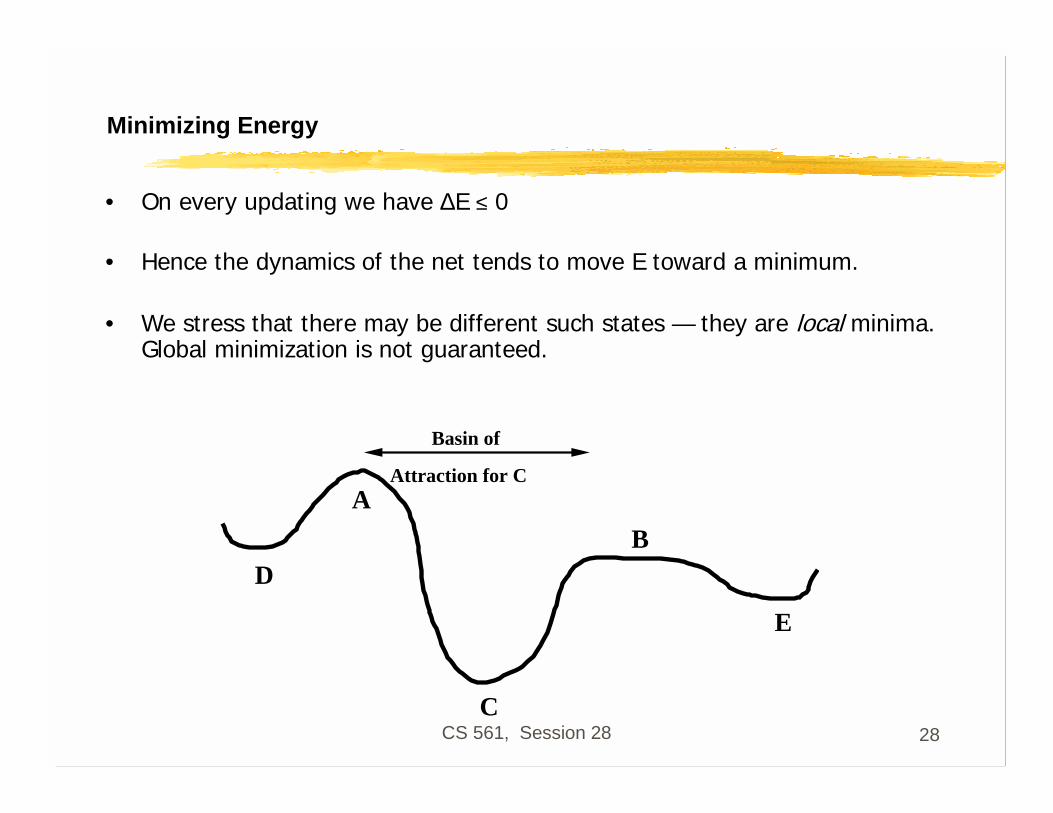
Minimizing Energy
• On every updating we have ∆E ≤ 0
• Hence the dynamics of the net tends to move E toward a minimum.
• We stress that there may be different such states — they are local minima. Global minimization is not guaranteed.
B
C
A
Basin of
Attraction for C
D
E

CS 561, Session 28 29
Self-Organizing Feature Maps
• The neural sheet is represented in a discretizedform by a (usually) 2-D lattice A of formal neurons.
• The input pattern is a vector x from some pattern space V. Inputvectors are normalized to unit length.
• The responsiveness of a neuron at a site r in A is measured by x.wr = Σi xi wri
where wr is the vector of the neuron's synaptic efficacies.
• The "image" of an external event is regarded as the unit with the maximal response to it

CS 561, Session 28 30
Self-Organizing Feature Maps
• Typical graphical representation: plot the weights (wr) as vertices and draw links between neurons that are nearest neighbors in A.
CS 561, Session 28 31
Self-Organizing Feature Maps
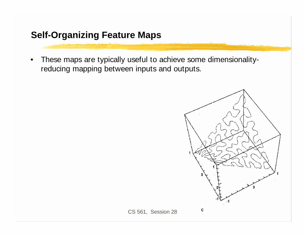
• These maps are typically useful to achieve some dimensionality-reducing mapping between inputs and outputs.

CS 561, Session 28 32
Applications: Classification
Business•Credit rating and risk assessment •Insurance risk evaluation •Fraud detection •Insider dealing detection •Marketing analysis•Mailshot profiling •Signature verification •Inventory control
Engineering•Machinery defect diagnosis •Signal processing •Character recognition •Process supervision •Process fault analysis •Speech recognition •Machine vision •Speech recognition •Radar signal classification
Security•Face recognition •Speaker verification •Fingerprint analysis
Medicine•General diagnosis •Detection of heart defects
Science•Recognising genes •Botanical classification •Bacteria identification

CS 561, Session 28 33
Applications: Modelling
Business•Prediction of share and commodity prices •Prediction of economic indicators •Insider dealing detection •Marketing analysis•Mailshot profiling •Signature verification •Inventory control
Engineering•Transducer linerisation •Colour discrimination •Robot control and navigation •Process control •Aircraft landing control •Car active suspension control •Printed Circuit auto routing •Integrated circuit layout •Image compression
Science•Prediction of the performance of drugs from the molecular structure •Weather prediction •Sunspot prediction
Medicine•. Medical imaging and image processing

CS 561, Session 28 34
Applications: Forecasting
•Future sales •Production Requirements •Market Performance •Economic Indicators •Energy Requirements •Time Based Variables

CS 561, Session 28 35
Applications: Novelty Detection
•Fault Monitoring •Performance Monitoring •Fraud Detection •Detecting Rate Features •Different Cases

CS 561, Session 28 36
Multi-layer Perceptron Classifier

CS 561, Session 28 37
http://ams.egeo.sai.jrc.it/eurostat/Lot16-SUPCOM95/node7.html
Multi-layer PerceptronClassifier

CS 561, Session 28 38
Classifiers
• http://www.electronicsletters.com/papers/2001/0020/paper.asp
• 1-stage approach
• 2-stageapproach

CS 561, Session 28 39
Example: face recognition
• Here using the 2-stage approach:

CS 561, Session 28 40
Training
• http://www.neci.nec.com/homepages/lawrence/papers/face-tr96/latex.html

CS 561, Session 28 41
Learning rate

CS 561, Session 28 42
Testing / Evaluation
• Look at performance as a function of network complexity

CS 561, Session 28 43
Testing / Evaluation
• Comparison with other known techniques

CS 561, Session 28 44
Associative Memories
• http://www.shef.ac.uk/psychology/gurney/notes/l5/l5.html
• Idea: store:
So that we can recover it if presented with corrupted data such as:

CS 561, Session 28 45
Associative memory with Hopfield nets
• Setup a Hopfield net such that local minima correspondto the stored patterns.
• Issues:- because of weight symmetry, anti-patterns (binary reverse) are stored as well as the original patterns (also spurious local minima are created when many patterns are stored)- if one tries to store more than about 0.14*(number of neurons)patterns, the network exhibits unstable behavior- works well only if patterns are uncorrelated
CS 561, Session 28 46
Capabilities and Limitations of Layered Networks
• Issues:
- what can given networks do?- What can they learn to do?- How many layers required for given task?- How many units per layer?- When will a network generalize?- What do we mean by generalize?- …
CS 561, Session 28 47
Capabilities and Limitations of Layered Networks
• What about boolean functions?
• Single-layer perceptrons are very limited:- XOR problem- etc.
• But what about multilayer perceptrons?
We can represent any boolean function with a network with just one hidden layer.
How??
CS 561, Session 28 48
Capabilities and Limitations of Layered Networks
To approximate a set of functions of the inputs by a layered network with continuous-valued units and sigmoidal activation function…
Cybenko, 1988: … at most two hidden layers are necessary, with arbitrary accuracy attainable by adding more hidden units.
Cybenko, 1989: one hidden layer is enough to approximate any continuous function.
Intuition of proof: decompose function to be approximated into a sum of localized “bumps.” The bumps can be constructed with two hidden layers.
Similar in spirit to Fourier decomposition. Bumps = radial basisfunctions.

CS 561, Session 28 49
Optimal Network Architectures
How can we determine the number of hidden units?
-genetic algorithms: evaluate variations of the network, using a metric that combines its performance and its complexity. Then apply various mutations to the network (change number of hidden units) until the best one is found.
-Pruning and weight decay:- apply weight decay (remember reinforcement learning) during training- eliminate connections with weight below threshold- re-train
- How about eliminating units? For example, eliminate units with total synaptic input weight smaller than threshold.
CS 561, Session 28 50
For further information
• See
Hertz, Krogh & Palmer: Introduction to the theory of neural computation (Addison Wesley)
In particular, the end of chapters 2 and 6.