Embed Size (px)
Citation preview
Artificial Neural Network Learning---
A Comparative Review
Costas NeocleousHigher Technical Institute, Cyprus
Christos SchizasUniversity of Cyprus, Cyprus
This is an attempt to present an organized review of learning techniques as used in neural networks, classified according to basic characteristics such as functionality, applicability, chronology, etc.
Outline
OutlineThe main objectives are:
To identify and appraise the important rules and to establish precedence.
To identify the basic characteristics of learning as applied to neural networks and propose a taxonomy.
Identify what is a generic rule and what is a special case. To critically compare various learning procedures. To gain a global overview of the subject area, and hence
explore the possibilities for novel and more effective rules or for novel implementations of the existing rules by applying them in new network structures or strategies.
Attempt a systematic organization and generalization of the various neural network learning rules.
These have been implemented with different approaches or tools such as basic mathematics, statistics, logical structures, neural structures, information theory, evolutionary systems, artificial life, and heuristics
IntroductionAn abundance of learning rules and procedures, both in the general ARTIFICIAL INTELLIGENCE context and in specific subfields of machine learning and neural networks exist
Many of the rules can be identified to be special cases of more generalized ones. Their variation is usually minor. Typically, they are given a different name or simply of different terminology and symbolism
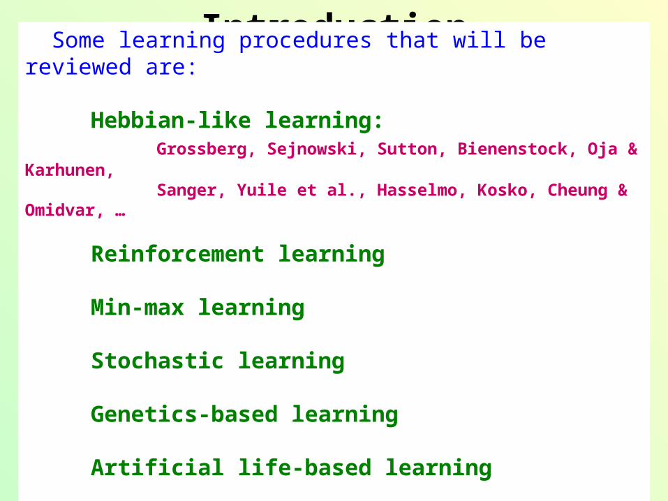
Introduction Some learning procedures that will be reviewed are:
Hebbian-like learning:Grossberg, Sejnowski, Sutton, Bienenstock, Oja & Karhunen, Sanger, Yuile et al., Hasselmo, Kosko, Cheung & Omidvar, …
Reinforcement learning
Min-max learning
Stochastic learning
Genetics-based learning
Artificial life-based learning
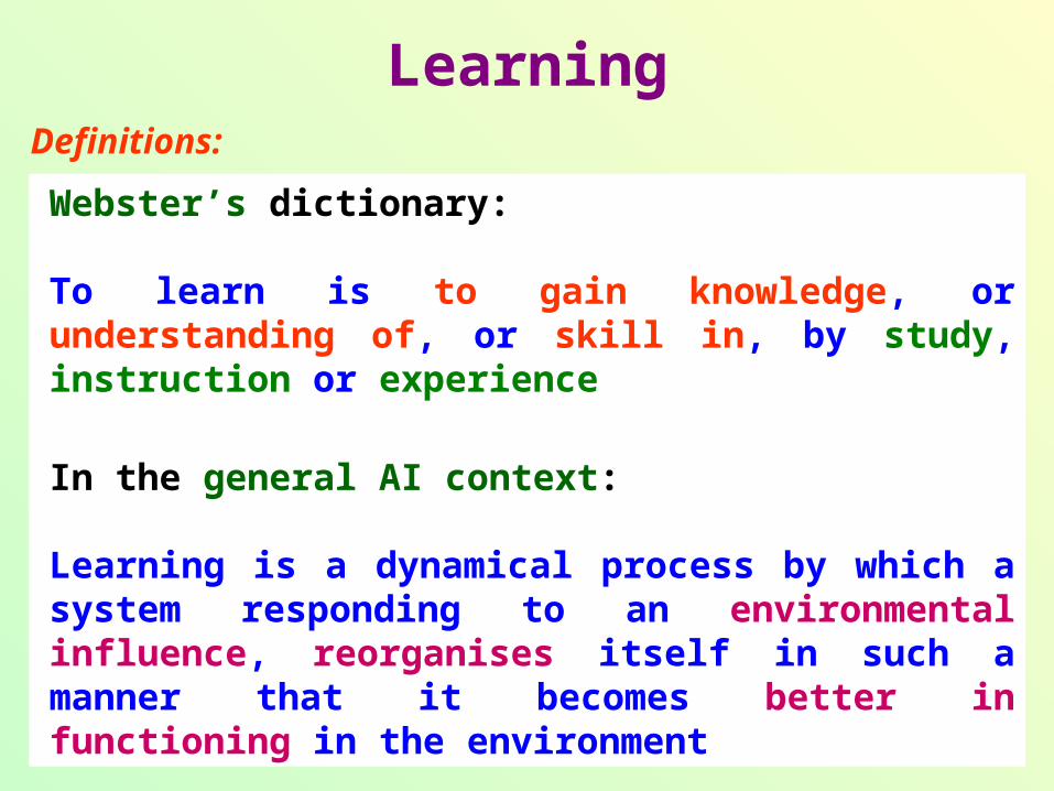
Webster’s dictionary:
To learn is to gain knowledge, or understanding of, or skill in, by study, instruction or experience
LearningDefinitions:
In the general AI context:
Learning is a dynamical process by which a system responding to an environmental influence, reorganises itself in such a manner that it becomes better in functioning in the environment
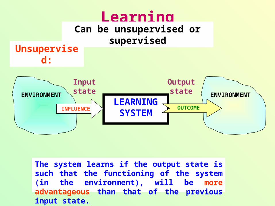
LearningCan be unsupervised or supervised
Unsupervised:
ENVIRONMENTLEARNING
SYSTEM
Input state
INFLUENCE
ENVIRONMENT
Output state
The system learns if the output state is such that the functioning of the system (in the environment), will be more advantageous than that of the previous input state.
OUTCOME
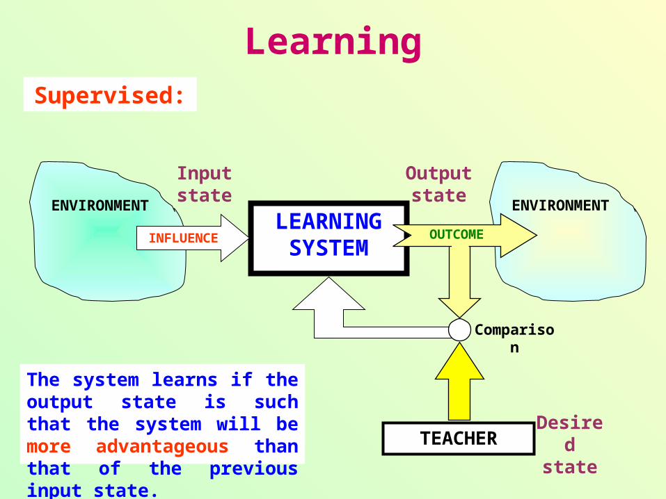
Supervised:
LEARNINGSYSTEM
Input state
ENVIRONMENT
INFLUENCE
ENVIRONMENT
OUTCOME
TEACHER
Comparison
Desired state
Learning
Output state
The system learns if the output state is such that the system will be more advantageous than that of the previous input state.
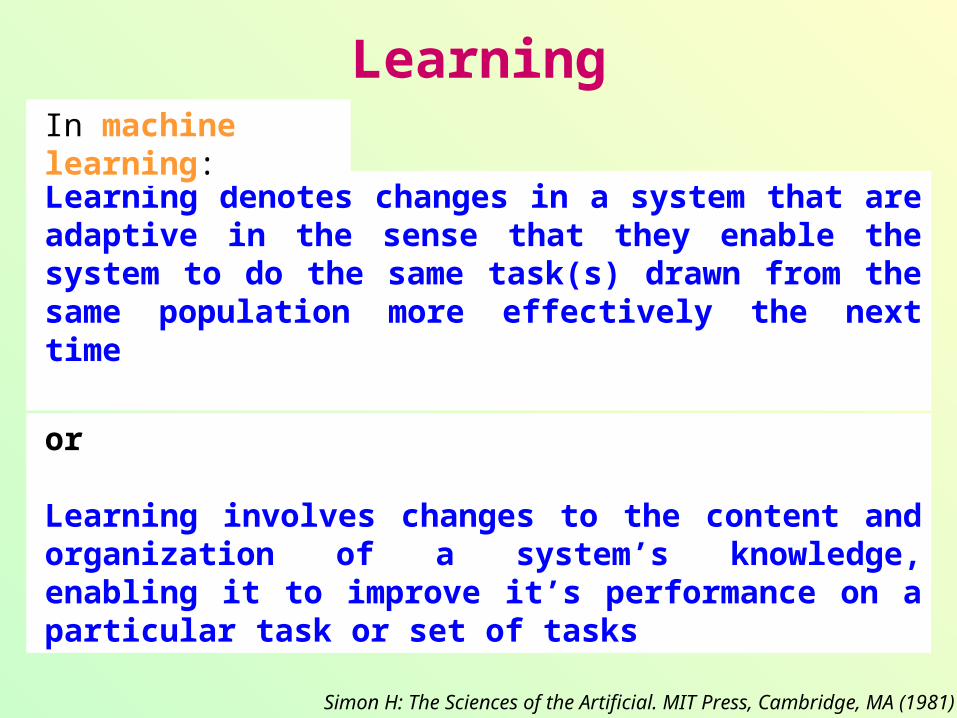
Learning denotes changes in a system that are adaptive in the sense that they enable the system to do the same task(s) drawn from the same population more effectively the next time
Simon H: The Sciences of the Artificial. MIT Press, Cambridge, MA (1981)
Learning
In machine learning:
or
Learning involves changes to the content and organization of a system’s knowledge, enabling it to improve it’s performance on a particular task or set of tasks
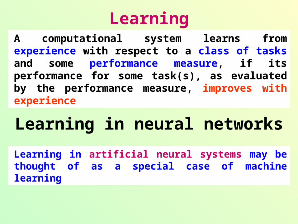
A computational system learns from experience with respect to a class of tasks and some performance measure, if its performance for some task(s), as evaluated by the performance measure, improves with experience
Learning in artificial neural systems may be thought of as a special case of machine learning
Learning in neural networks
Learning
Learning in neural networks
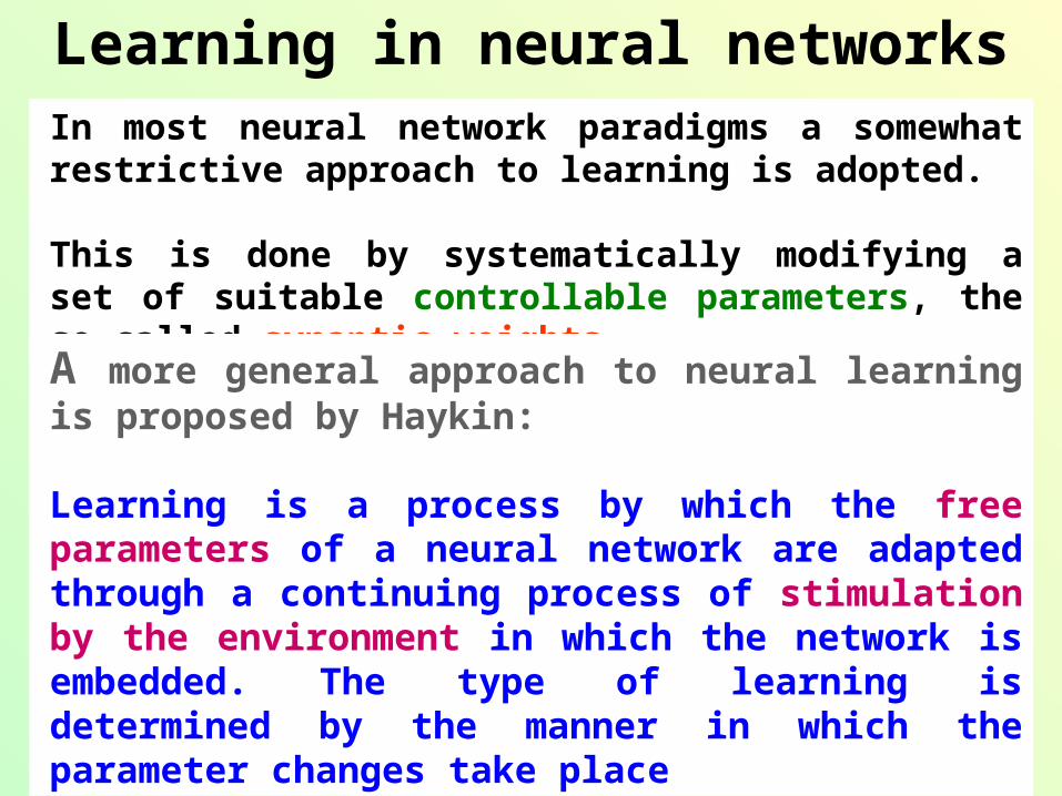
In most neural network paradigms a somewhat restrictive approach to learning is adopted.
This is done by systematically modifying a set of suitable controllable parameters, the so-called synaptic weights.
A more general approach to neural learning is proposed by Haykin:
Learning is a process by which the free parameters of a neural network are adapted through a continuing process of stimulation by the environment in which the network is embedded. The type of learning is determined by the manner in which the parameter changes take place
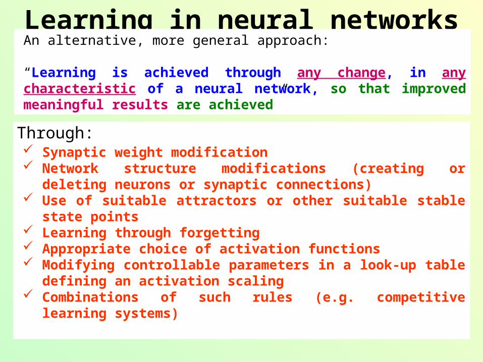
Learning in neural networksAn alternative, more general approach:
“Learning is achieved through any change, in any characteristic of a neural network, so that improved meaningful results are achieved”
Synaptic weight modification Network structure modifications (creating or deleting neurons or
synaptic connections) Use of suitable attractors or other suitable stable state points Learning through forgetting Appropriate choice of activation functions Modifying controllable parameters in a look-up table defining an
activation scaling Combinations of such rules (e.g. competitive learning systems)
Through:
Learning as optimization
The majority of learning rules are such that a desired objective is met by a procedure of minimizing a suitable associated criterion (also known as Computational energy, Lyapunov function, or Hamilton function), whenever such exists or may be constructed, in a manner similar to the optimization procedures.
Learning as optimization
Many methods have been proposed for the implementation of the desired minimization, such as
0th order1st order gradient-descent (Newton’s, Steepest-descent)Damped Newton (Levenberg-Marquardt)Quasi-Newton (Broyden-Fletcher-Goldfarb-Shanno, Barnes-Rosen) Conjugate gradient methods
Many of these rules are special cases of a generalized unconstrained optimization procedure, briefly described:
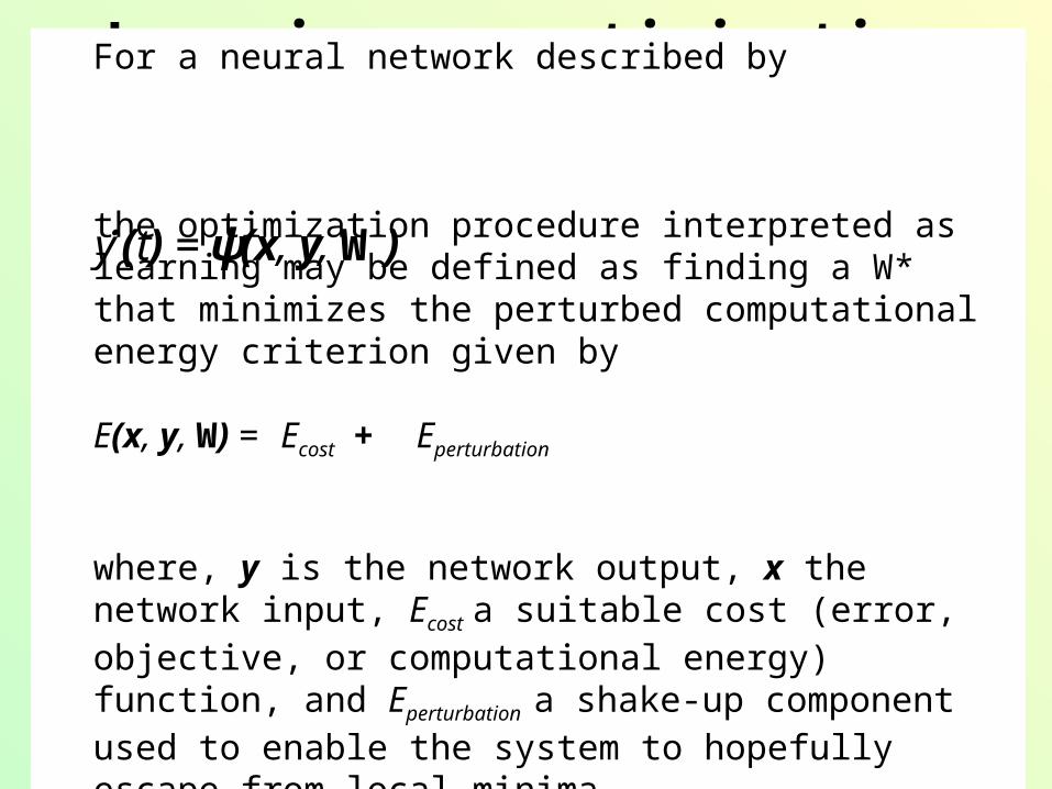
Learning as optimizationFor a neural network described by
the optimization procedure interpreted as learning may be defined as finding a W* that minimizes the perturbed computational energy criterion given by
E(x, y, W) = Ecost + Eperturbation
where, y is the network output, x the network input, Ecost a suitable cost (error, objective, or computational energy) function, and Eperturbation a shake-up component used to enable the system to hopefully escape from local minima.
y (t) = ψ(x, y, W)
Learning as optimizationIf E is continuous in the domain of interest, the minima of E with respect to the adaptable parameter (weights), W, are obtained when the gradient of E is zero, or when: wE = 0
An exact solution of above is not easily obtained an it is not usually sought.
Different, non-analytical methods for finding the minima of E have been proposed as neural learning rules. These are mainly implemented as iterative procedures suitable for computer simulations.
Learning as optimization
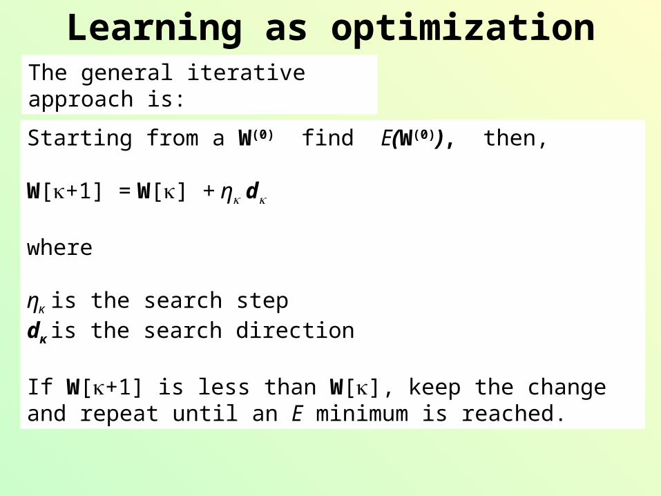
The general iterative approach is:
Starting from a W(0) find E(W(0)), then,
W[+1] = W[] + η d
where
ηκ is the search step dκ is the search direction
If W[+1] is less than W[], keep the change and repeat until an E minimum is reached.
Learning as optimization
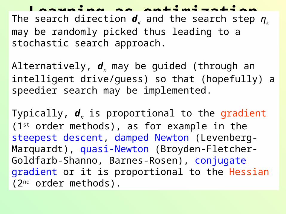
The search direction d and the search step η may be randomly picked thus leading to a stochastic search approach.
Alternatively, d may be guided (through an intelligent drive/guess) so that (hopefully) a speedier search may be implemented.
Typically, d is proportional to the gradient (1st order methods), as for example in the steepest descent, damped Newton (Levenberg-Marquardt), quasi-Newton (Broyden-Fletcher-Goldfarb-Shanno, Barnes-Rosen), conjugate gradient or it is proportional to the Hessian (2nd order methods).
Learning as optimization
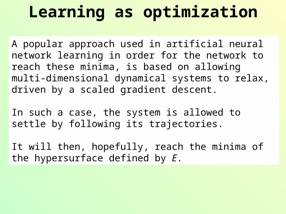
A popular approach used in artificial neural network learning in order for the network to reach these minima, is based on allowing multi-dimensional dynamical systems to relax, driven by a scaled gradient descent.
In such a case, the system is allowed to settle by following its trajectories.
It will then, hopefully, reach the minima of the hypersurface defined by E.
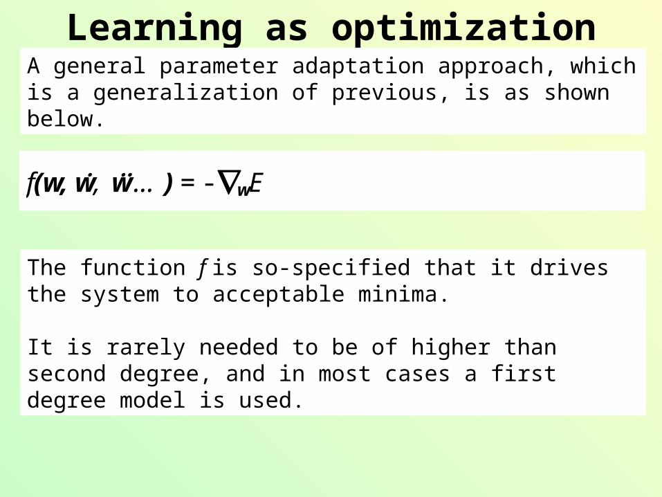
Learning as optimizationA general parameter adaptation approach, which is a generalization of previous, is as shown below.
f(w, w , w … ) = - wE
The function f is so-specified that it drives the system to acceptable minima.
It is rarely needed to be of higher than second degree, and in most cases a first degree model is used.
Learning as optimization
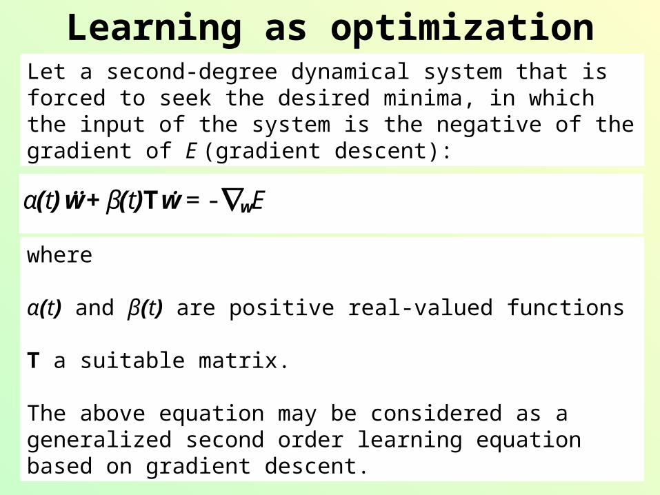
Let a second-degree dynamical system that is forced to seek the desired minima, in which the input of the system is the negative of the gradient of E (gradient descent):
where
α(t) and β(t) are positive real-valued functions
T a suitable matrix.
The above equation may be considered as a generalized second order learning equation based on gradient descent.
α(t) w + β(t)Tw = - wE
Learning as optimization
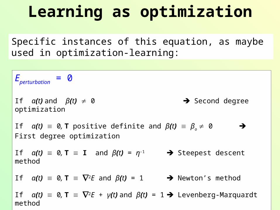
Specific instances of this equation, as maybe used in optimization-learning:
Eperturbation = 0
If α(t) and β(t) 0 Second degree optimization
If α(t) 0, T positive definite and β(t) βο 0 First degree optimization
If α(t) 0, T I and β(t) = η-1 Steepest descent method
If α(t) 0, T 2E and β(t) = 1 Newton’s method
If α(t) 0, T 2E + γ(t) and β(t) = 1 Levenberg-Marquardt method
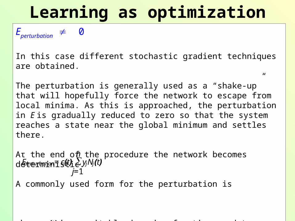
Learning as optimizationEperturbation 0
In this case different stochastic gradient techniques are obtained.
The perturbation is generally used as a “shake-up” that will hopefully force the network to escape from local minima. As this is approached, the perturbation in E is gradually reduced to zero so that the system reaches a state near the global minimum and settles there.
Ατ the end of the procedure the network becomes deterministic.
A commonly used form for the perturbation is
where c(t) is a suitable decaying function used to gradually reduce the effects of noise and Nj(t) is noise applied to each neuron j.
Eperturbation = c(t) j=1
n yjNj(t)
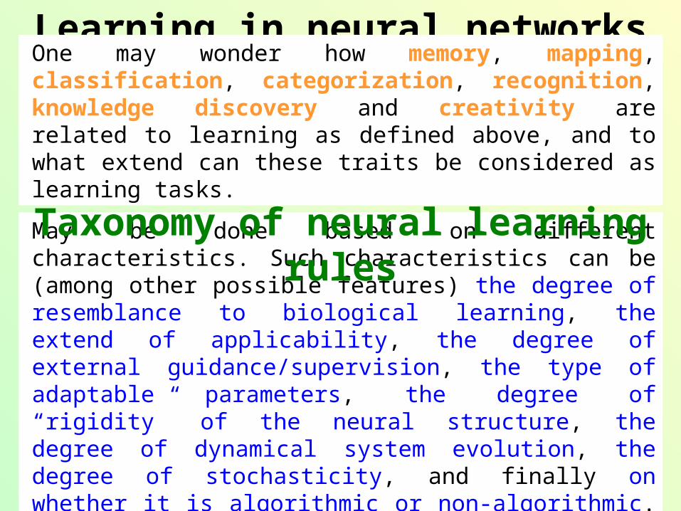
Learning in neural networksOne may wonder how memory, mapping, classification, categorization, recognition, knowledge discovery and creativity are related to learning as defined above, and to what extend can these traits be considered as learning tasks.
May be done based on different characteristics. Such characteristics can be (among other possible features) the degree of resemblance to biological learning, the extend of applicability, the degree of external guidance/supervision, the type of adaptable parameters, the degree of “rigidity” of the neural structure, the degree of dynamical system evolution, the degree of stochasticity, and finally on whether it is algorithmic or non-algorithmic.
Taxonomy of neural learning rules
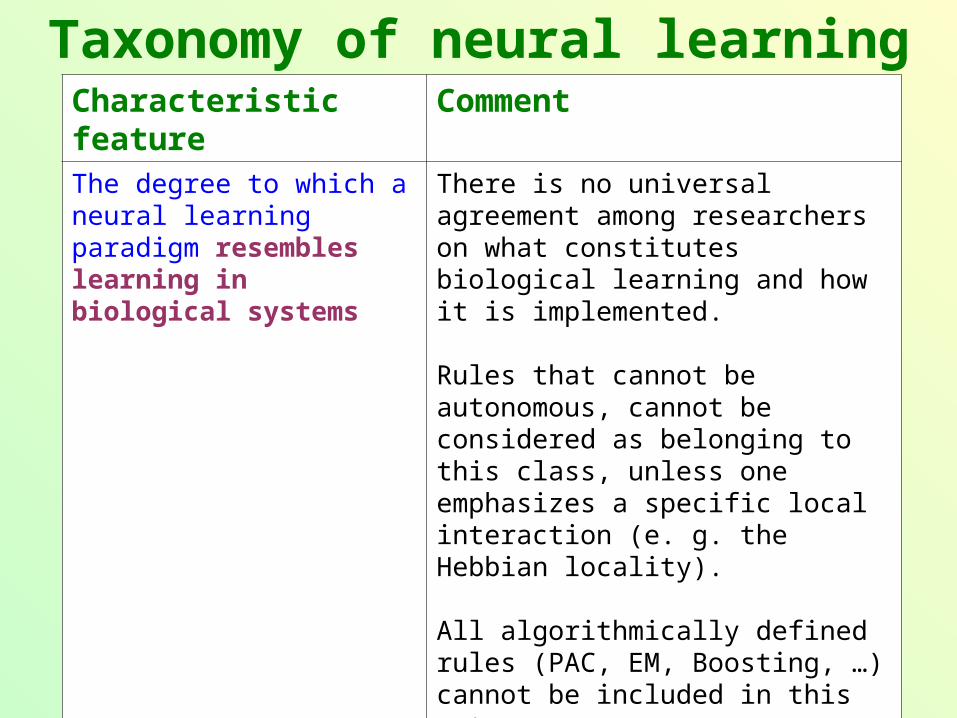
Taxonomy of neural learning rules Characteristic feature CommentThe degree to which a neural learning paradigm resembles learning in biological systems
There is no universal agreement among researchers on what constitutes biological learning and how it is implemented.
Rules that cannot be autonomous, cannot be considered as belonging to this class, unless one emphasizes a specific local interaction (e. g. the Hebbian locality).
All algorithmically defined rules (PAC, EM, Boosting, …) cannot be included in this category.
Typical rules of the class are the basic Hebbian, as well as Hebbian-like rules used in spiking neuron networks.
Taxonomy of neural learning rules
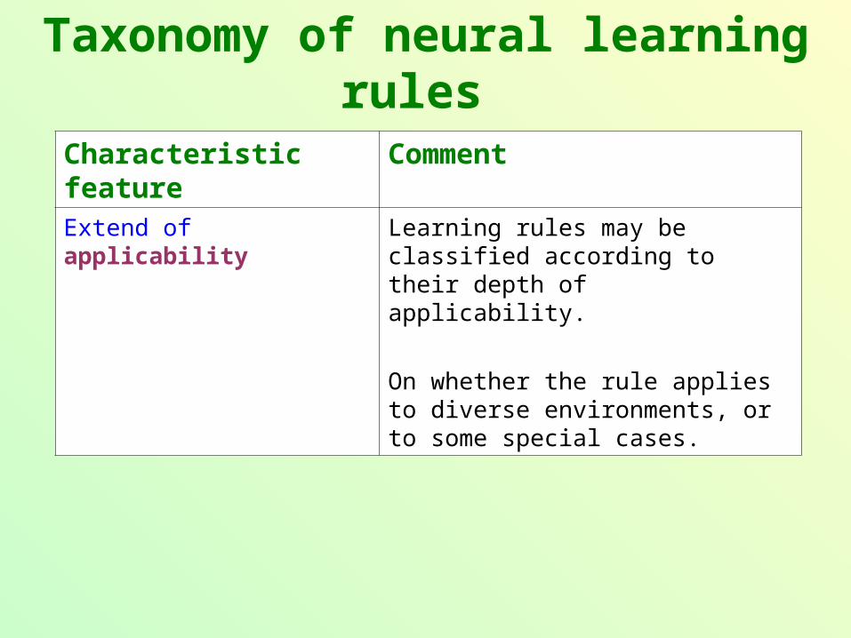
Characteristic feature CommentExtend of applicability Learning rules may be classified
according to their depth of applicability.
On whether the rule applies to diverse environments, or to some special cases.
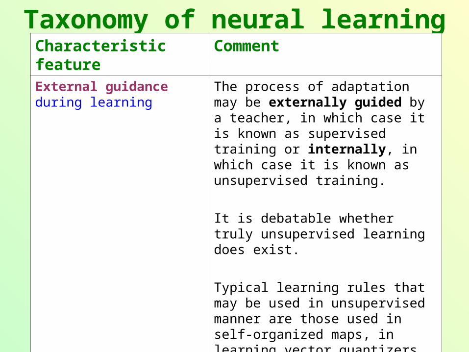
Taxonomy of neural learning rules Characteristic feature CommentExternal guidance during learning
The process of adaptation may be externally guided by a teacher, in which case it is known as supervised training or internally, in which case it is known as unsupervised training.
It is debatable whether truly unsupervised learning does exist.
Typical learning rules that may be used in unsupervised manner are those used in self-organized maps, in learning vector quantizers, in principal component analysis (PCA) and in independent component analysis (ICA) procedures.
Taxonomy of neural learning rules
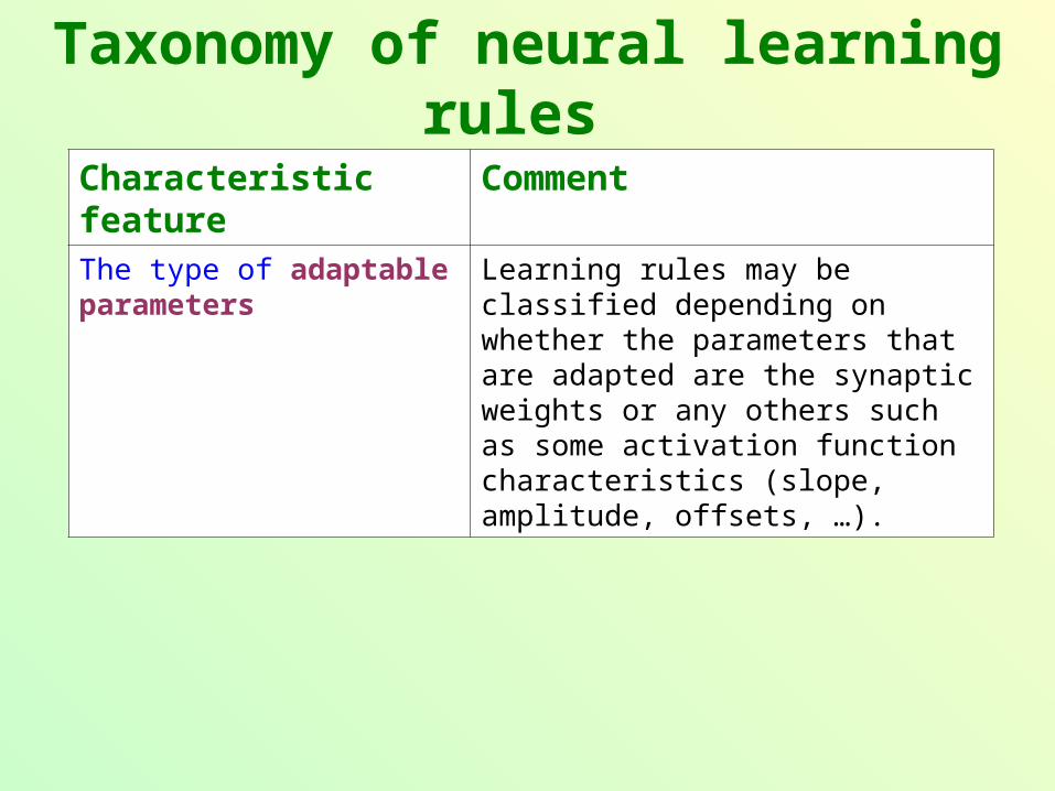
Characteristic feature CommentThe type of adaptable parameters
Learning rules may be classified depending on whether the parameters that are adapted are the synaptic weights or any others such as some activation function characteristics (slope, amplitude, offsets, …).
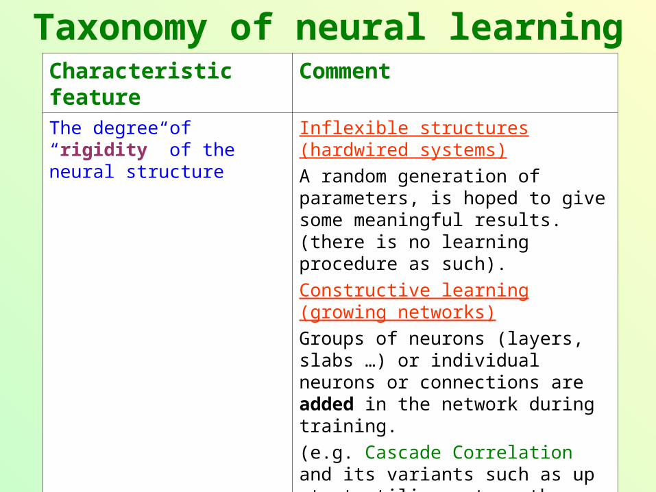
Taxonomy of neural learning rules Characteristic feature CommentThe degree of “rigidity” of the neural structure
Inflexible structures (hardwired systems)
A random generation of parameters, is hoped to give some meaningful results. (there is no learning procedure as such).
Constructive learning (growing networks)
Groups of neurons (layers, slabs …) or individual neurons or connections are added in the network during training.
(e.g. Cascade Correlation and its variants such as up start, tiling, etc., the Boosting algorithm, …)
Destructive learning (shrinking networks)
Groups of neurons (layers, slabs …) or individual processing units (neurons) or connections are removed from a network during training (pruning)
Taxonomy of neural learning rules
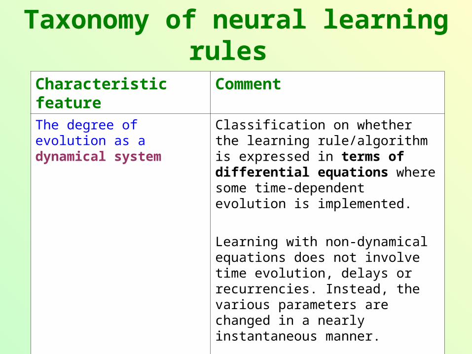
Characteristic feature CommentThe degree of evolution as a dynamical system
Classification on whether the learning rule/algorithm is expressed in terms of differential equations where some time-dependent evolution is implemented.
Learning with non-dynamical equations does not involve time evolution, delays or recurrencies. Instead, the various parameters are changed in a nearly instantaneous manner.
Taxonomy of neural learning rules
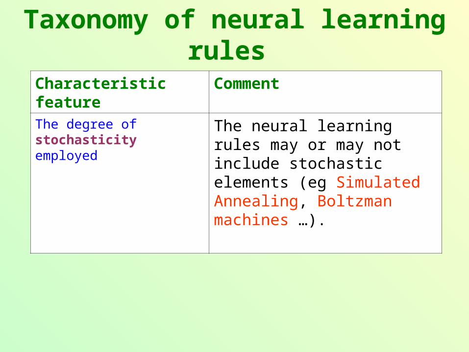
Characteristic feature CommentThe degree of stochasticity employed
The neural learning rules may or may not include stochastic elements (eg Simulated Annealing, Boltzman machines …).
Taxonomy of neural learning rules
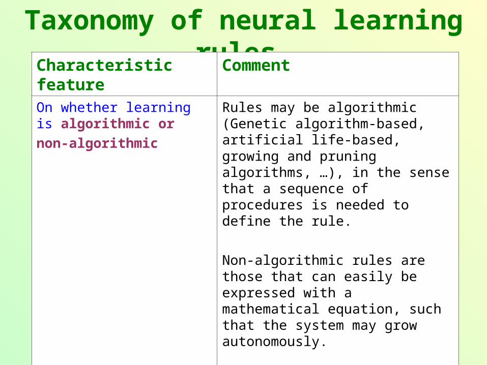
Characteristic feature CommentOn whether learning is algorithmic or
non-algorithmic
Rules may be algorithmic (Genetic algorithm-based, artificial life-based, growing and pruning algorithms, …), in the sense that a sequence of procedures is needed to define the rule.
Non-algorithmic rules are those that can easily be expressed with a mathematical equation, such that the system may grow autonomously.
This is a rather artificial distinction, and from a practical point of view, the end result is what counts most.
Taxonomy of neural learning rules
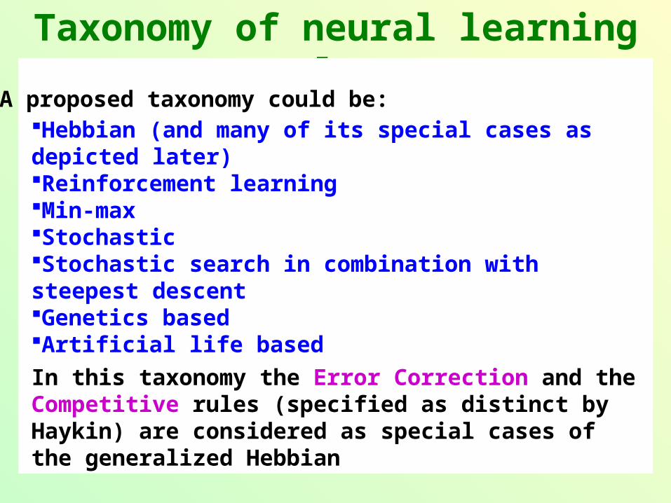
Hebbian (and many of its special cases as depicted later)Reinforcement learningMin-max Stochastic Stochastic search in combination with steepest descentGenetics based Artificial life based
In this taxonomy the Error Correction and the Competitive rules (specified as distinct by Haykin) are considered as special cases of the generalized Hebbian
A proposed taxonomy could be:
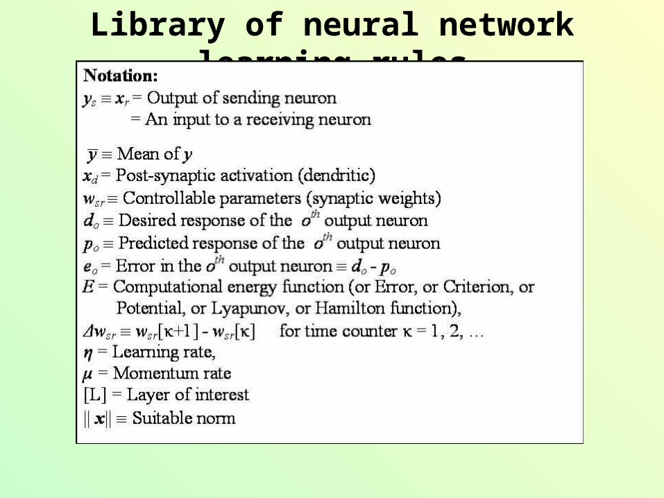
Library of neural network learning rules
Library of neural network learning rulesMAJOR GROUP RULE
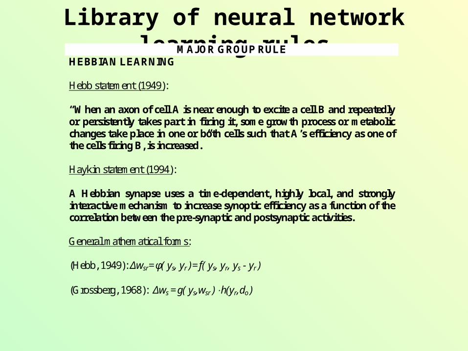
HEBBIAN LEARNING Hebb statement (1949): “When an axon of cell A is near enough to excite a cell B and repeatedly or persistently takes part in firing it, some growth process or metabolic changes take place in one or both cells such that A’s efficiency as one of the cells firing B, is increased.” Haykin statement (1994): A Hebbian synapse uses a time-dependent, highly local, and strongly interactive mechanism to increase synoptic efficiency as a function of the correlation between the pre-synaptic and postsynaptic activities. General mathematical forms: (Hebb, 1949): Δwsr=φ( ys, yr )=f( ys, yr, ys - yr ) (Grossberg, 1968): Δws =g( ys,wsr ) h(yr,do )
Library of neural network learning rules
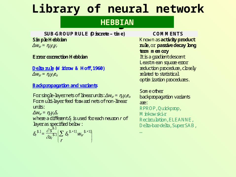
SUB-GROUP RULE (Discrete – time) COMMENTS Simple Hebbian Δwsr = ηrysyr
Known as activity product rule, or passive decay long term memory
Error correction Hebbian Delta rule (Widrow & Hoff, 1960) Δwsr = ηryseo Backpropagation and variants
For single-layer nets of linear units: Δwsr = ηryseo For multi-layer feed forward nets of non-linear units: Δwsr = ηrysδr
where a different δj is used for each neuron r of layer as specified below:
δr[L]
= s
[L]
ur[L]
r δr
[L+1] wsr
[L+1]
It is a gradient descent Least mean square error reduction procedure, closely related to statistical optimization procedures. Some other backpropagation variants are: RPROP, Quickprop, Minkowski-r Recirculation, ELEANNE, Delta-bar-delta, Super SAB, …
HEBBIAN
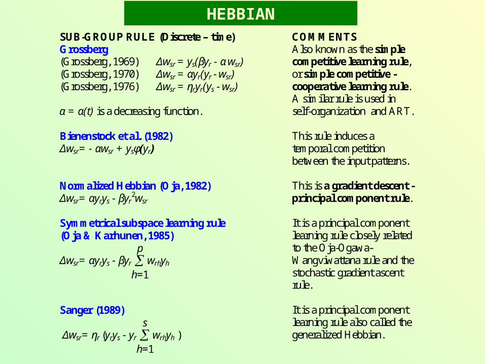
SUB-GROUP RULE (Discrete – time) COMMENTS Grossberg (Grossberg, 1969) Δwsr = ys(βyr - α wsr) (Grossberg, 1970) Δwsr = αyr(yr - wsr) (Grossberg, 1976) Δwsr = ηryr(ys - wsr) α = α(t) is a decreasing function.
Also known as the simple competitive learning rule, or simple competitive - cooperative learning rule. A similar rule is used in self-organization and ART.
Bienenstock et al. (1982) Δwsr= - αwsr + ysφ(yr)
This rule induces a temporal competition between the input patterns.
Normalized Hebbian (Oja, 1982) Δwsr= αyrys - βyr
2wsr This is a gradient descent - principal component rule.
Symmetrical subspace learning rule (Oja & Karhunen, 1985)
Δwsr= αyrys - βyr h=1
p wrhyh
It is a principal component learning rule closely related to the Oja-Ogawa-Wangviwattana rule and the stochastic gradient ascent rule.
Sanger (1989)
Δwsr= ηr (yrys - yr h=1
s wrhyh )
It is a principal component learning rule also called the generalized Hebbian.
HEBBIAN
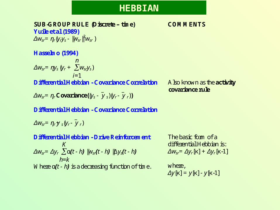
HEBBIAN
SUB-GROUP RULE (Discrete – time) COMMENTS Yuile et al (1989) Δwsr= ηr(yrys - ||wsr||
2wsr )
Hasselmo (1994)
Δwsr= ηys (yr + i=1
nwsrys)
Differential Hebbian - Covariance Correlation
Δwsr= ηr Covariance((ys - y _
s)(yr - y _
r))
Also known as the activity covariance rule
Differential Hebbian - Covariance Correlation
Δwsr= ηr y _ s(yr - y
_ r)
Differential Hebbian - Drive Reinforcement
Δwsr= Δyr h=k
Kα(t - h) ||wsr(t - h) ||Δys(t - h)
Where α(t - h) is a decreasing function of time.
The basic form of a differential Hebbian is: Δwsr= Δyr[κ] + Δyr[κ-1] where, Δy[κ] = y[κ] - y[κ-1]
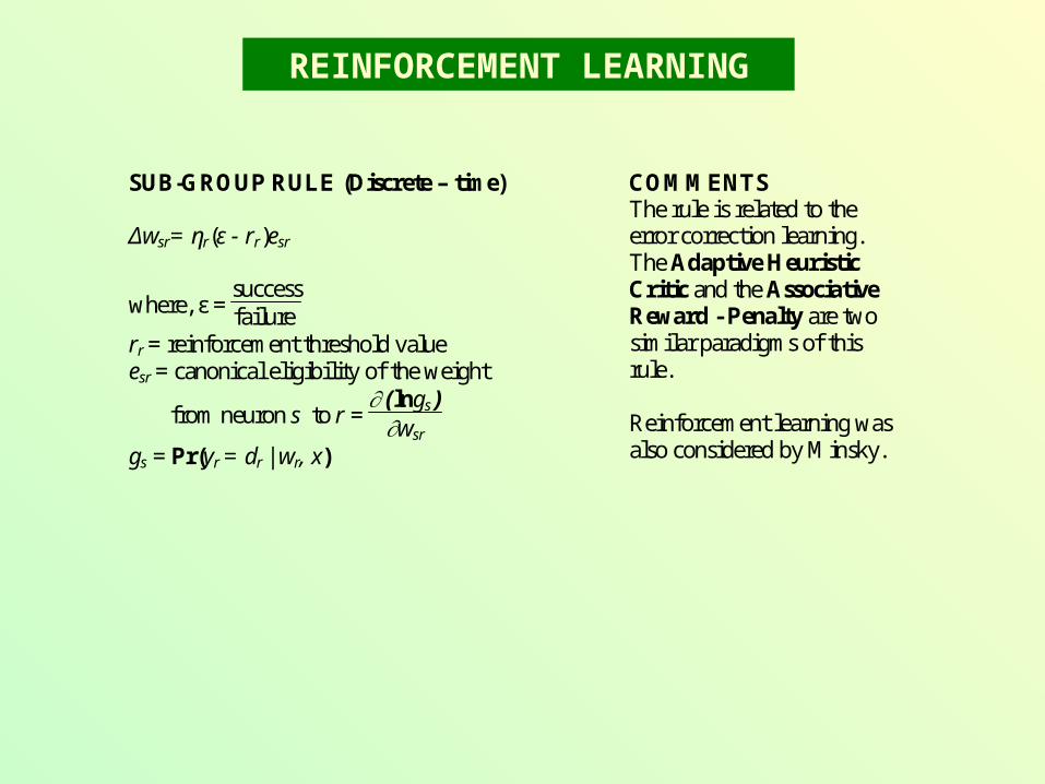
REINFORCEMENT LEARNING
SUB-GROUP RULE (Discrete – time) COMMENTS Δwsr= ηr(ε - rr)esr
where, ε = successfailure
rr = reinforcement threshold value esr = canonical eligibility of the weight
from neuron s to r = (lngs )
wsr
gs = Pr(yr = dr | wr, x)
The rule is related to the error correction learning. The Adaptive Heuristic Critic and the Associative Reward - Penalty are two similar paradigms of this rule. Reinforcement learning was also considered by Minsky.
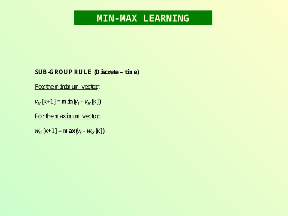
MIN-MAX LEARNING
SUB-GROUP RULE (Discrete – time) For the minimum vector: vsr[κ+1] = min(ys - vsr[κ]) For the maximum vector: wsr[κ+1] = max(ys - wsr[κ])
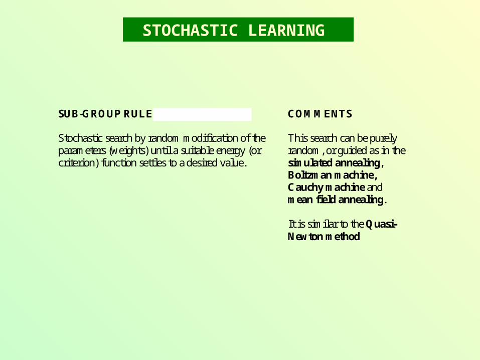
STOCHASTIC LEARNING
SUB-GROUP RULE (Discrete – time) COMMENTS Stochastic search by random modification of the parameters (weights) until a suitable energy (or criterion) function settles to a desired value.
This search can be purely random, or guided as in the simulated annealing, Boltzman machine, Cauchy machine and mean field annealing. It is similar to the Quasi-Newton method

STOCHASTIC HEBBIAN
SUB-GROUP RULE (Discrete – time) Hebbian Annealing A stochastic local Hebbian rule in which the weights are changed depending on their score in a suitable function.
GENETICS BASED LEARNING
Evolutionary techniques (genetic algorithms) are used to find weights and other parameters, or to prune or grow neural structures
ARTIFICIAL LIFE BASED LEARNING
The particle swarm optimizer is one such learning procedure
Concluding remarks
The problem of neural system learning is ultimately very important in the sense that evolvable intelligence can emerge when the learning procedure is automatic and unsupervised.
The rules mostly used by researchers and application users are of gradient descent type
They are closely related to optimization techniques developed by mathematicians, statisticians and researchers working mainly in the field of “operations research”
A systematic examination of the effectiveness of these rules is a matter of extensive research being conducted at different research centers. Conclusive comparative findings on the relative merits of each learning rule are not presently available.
Concluding remarks
The term “unsupervised” is debatable depending on the level of scrutiny applied when evaluating a rule. It is customary to consider some learning as unsupervised when there is no specific and well defined external teacher
In the so-called self-organizing systems, the system organizes apparently unrelated data into sets of more meaningful packets of information
Ultimately though, how can intelligent organisms learn in total isolation? Looking at supervisability in more liberal terms, one could say that learning is not well-specified supervised or unsupervised procedure. It is rather a complicated system of individual processes that jointly help in manifesting an emergent behavior that “learns” from experience