Artifacts in magnetic measurements of fluid samplesZ. Boekelheide and C. L. Dennis Citation: AIP Advances 6, 085201 (2016); doi: 10.1063/1.4960457 View online: http://dx.doi.org/10.1063/1.4960457 View Table of Contents: http://scitation.aip.org/content/aip/journal/adva/6/8?ver=pdfcov Published by the AIP Publishing Articles you may be interested in Spherical sample holders to improve the susceptibility measurement of superparamagnetic materials Rev. Sci. Instrum. 83, 045106 (2012); 10.1063/1.3700185 Optimization of the first order gradiometer for small sample magnetization measurements using pulseintegrating magnetometer Rev. Sci. Instrum. 80, 104702 (2009); 10.1063/1.3239404 Design of a compensated signal rod for low magnetic moment sample measurements with a vibrating samplemagnetometer Rev. Sci. Instrum. 79, 035107 (2008); 10.1063/1.2901602 Vector vibrating-sample magnetometer with permanent magnet flux source J. Appl. Phys. 99, 08D912 (2006); 10.1063/1.2170595 Anisotropy characterization of garnet films by using vibrating sample magnetometer measurements J. Appl. Phys. 93, 7065 (2003); 10.1063/1.1540142

Reuse of AIP Publishing content is subject to the terms at: https://publishing.aip.org/authors/rights-and-permissions. Download to IP: 139.147.54.99 On: Mon, 01 Aug

2016 14:24:09

AIP ADVANCES 6, 085201 (2016)

Artifacts in magnetic measurements of fluid samplesZ. Boekelheide1,2,a and C. L. Dennis1,b1Material Measurement Laboratory, National Institute of Standards and Technology,Gaithersburg, Maryland 20899, USA2Department of Physics, Lafayette College, Easton PA 18042, USA

(Received 7 August 2015; accepted 24 July 2016; published online 1 August 2016)

Applications of magnetic fluids are ever increasing, as well as the correspondingneed to be able to characterize these fluids in situ. Commercial magnetometers areaccurate and well-characterized for solid and powder samples, but their use with fluidsamples is more limited. Here, we describe artifacts which can occur in magneticmeasurements of fluid samples and their impact. The most critical problem in themeasurement of fluid samples is the dynamic nature of the sample position andsize/shape. Methods to reduce these artifacts are also discussed, such as removal of airbubbles and dynamic centering. C 2016 Author(s). All article content, except whereotherwise noted, is licensed under a Creative Commons Attribution (CC BY) license(http://creativecommons.org/licenses/by/4.0/). [http://dx.doi.org/10.1063/1.4960457]

I. INTRODUCTION

Magnetic micro- and nanoparticles dispersed in fluids have many applications including damp-ing in vehicle suspensions and landing gear,1 and heat transfer materials.2 In biomedicine, they canbe used as contrast agents for magnetic resonance imaging (MRI)3 and magnetic particle imaging(MPI),4 as well as for magnetic nanoparticle hyperthermia.5 Magnetic fluids are even found inart, where they are used in certain art conservation processes.6 To optimize their behavior for thiswide range of applications, a complete understanding of the magnetic behavior of these fluids isrequired. Therefore, there is a need for accurate magnetic measurements of magnetic micro- andnano-particles in solution.

The details of the magnetic hysteresis loop (magnetic moment m as a function of appliedmagnetic field H) can be very different for nanoparticles suspended in a fluid than for dried orimmobilized nanoparticles.7 Nanoparticles suspended in fluid may rearrange with applied field,forming structures such as chains or loops due to their interaction with neighboring nanoparticles aswell as with the applied magnetic field.8,9 Nanoparticles may also rotate to align their magnetic easyaxis along the direction of the field.7 Both effects may change the effective magnetic anisotropy ofthe macroscopic fluid sample, which in turn affects the shape of the hysteresis loop. To capture theseeffects in magnetic measurements of fluids, it is necessary to measure the samples in their fluid form(“in situ”). Here we report on the magnetic characterization of magnetic micro- and nanoparticlesin fluids. We describe artifacts which may arise due to the fluid nature of the samples and suggestmethods to avoid them.

II. EQUIPMENT

Instruments for measuring the magnetic moment as a function of applied magnetic fieldinclude the alternating field gradient magnetometer (AGFM), the vibrating sample magnetometer(VSM)10 and superconducting quantum interference device (SQUID) magnetometer.11 While thesecan be built in-house,12 they are also commercially available.13 These commercial systems arewide-spread, with the measurement techniques and sample holders optimized for solid samples

aboekelhz@lafayette.edubcindi.dennis@nist.gov

2158-3226/2016/6(8)/085201/13 6, 085201-1 ©Author(s) 2016.

Reuse of AIP Publishing content is subject to the terms at: https://publishing.aip.org/authors/rights-and-permissions. Download to IP: 139.147.54.99 On: Mon, 01 Aug

2016 14:24:09

085201-2 Z. Boekelheide and C. L. Dennis AIP Advances 6, 085201 (2016)

like bulk crystals, thin films, and packed powders, but not for fluid samples. As a result, manyresearchers dry their fluid samples into powders or immobilize them in epoxy or another compositefor measurement. Alternatively, some researchers are focused on measuring single nanoparticleswith micro-SQUIDs14 or magneto-optical indicator films.15 However, these two single-nanoparticlemethods are (respectively) limited by their (1) access only to magnetic properties (i.e. saturationmagnetization) that do not depend on the presence of the fluid and (2) lack of good ensembleaveraging on the effect of interactions on magnetic fluid properties.

To focus on the previously described dynamic effects that arise from magnetic nanoparticlesin solution, we have used commercially available magnetometers, not single nanoparticle methods.Specifically, the results presented here are from an MPMS SQUID by Quantum Design and anMPMS3 SQUID-VSM by Quantum Design.13 Our results can be extended to other solid-samplemagnetometers such as the vibrating sample magnetometer. We have chosen these two instrumentsto demonstrate the issues with fluid samples due to their access to the raw data which includescentering information.13

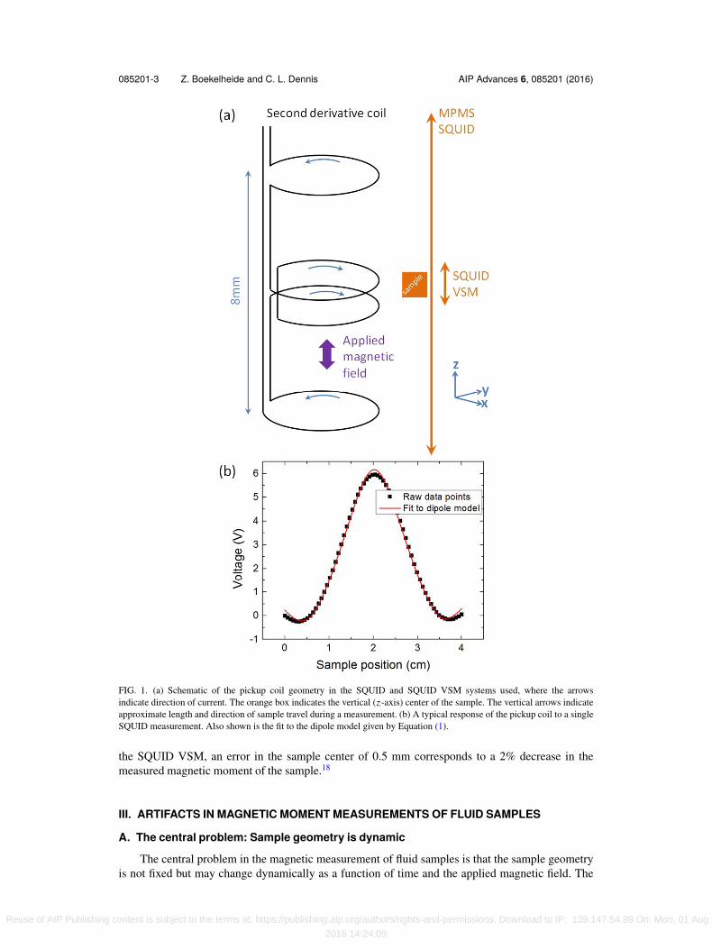
In all of these magnetometers, a sample is moved through or near a coil of wire. This coil ofwire can be made of copper or a superconductor. The changing magnetic field from the samplemoving induces a voltage in the coil (Faraday’s Law). Figure 1(a) shows the geometry of thesuperconducting pickup coil which is common to both systems used. This coil configuration (aka asecond derivative coil), is designed to eliminate contributions from magnetic fields which are eitherconstant, such as the applied magnetic field, or linear, such as a gradient in the applied magneticfield. Thus, any signal is only due to the 2nd derivative or higher order terms of the changingmagnetic field, i.e. the dipole field originating from the magnetic moment of the sample.11

The SQUID and SQUID VSM systems use similar detection coil geometry, but the measure-ment techniques are quite different. Prior to either measurement, the sample is positioned in themiddle of the coils horizontally (x-y plane) and vertically (z-axis). This position is called the“center”. In a SQUID measurement, the sample is then stepped vertically through the entire coil andthe induced voltage in the coil is measured at each step. This yields the “raw data”, an example ofwhich is shown in Figure 1(b). This induced voltage as a function of position f (z) is modeled as asingle point dipole:

f (z) = P1+P2z + P3

2[R2 + (z + P4)2]−3/2

−[R2 + (Λ + (z + P4))2]−3/2

−[R2 + (−Λ + (z + P4))2]−3/2,

(1)

where the parameters Λ and R refer to the coil separation and radius, respectively, and P1, P2, P3,and P4 are the four fit parameters of the dipole model. P3 is the amplitude of the induced voltage,which is proportional to the magnetic moment of the sample, and P4 is the center position. P1 is aconstant offset and P2 is a linear offset to account for drift in the SQUIDs.16

In a SQUID VSM measurement, instead of stepping the sample through the entire coil, which istime-intensive, the sample is vibrated vertically about the center point of the coil with an amplitudeof typically a few mm.17 The amplitude of the induced voltage is proportional to magnetic moment.(This is characteristic of a VSM measurement in general, although the coil configuration is differentin an electromagnet-based system.)

In a typical SQUID VSM measurement, the sample center position is determined initially bya measurement similar to a SQUID scan: the vibrating sample is moved through the coils and asingle maximum/minimum occurs where the sample is exactly centered between the coils. Thiscenter position is used for the rest of the measurement unless it is determined that the sampleshould be recentered, for example during a measurement that includes a temperature change andresulting change in length of the sample holder rod. “Dynamic centering” occurs when the sampleis re-centered prior to every measurement, but requires additional time. Since the induced voltageis maximized at the center position, errors in vertical sample centering lead to a decrease in themagnitude of the measured moment. This error varies with the offset from the true center. For

Reuse of AIP Publishing content is subject to the terms at: https://publishing.aip.org/authors/rights-and-permissions. Download to IP: 139.147.54.99 On: Mon, 01 Aug

2016 14:24:09

085201-3 Z. Boekelheide and C. L. Dennis AIP Advances 6, 085201 (2016)

FIG. 1. (a) Schematic of the pickup coil geometry in the SQUID and SQUID VSM systems used, where the arrowsindicate direction of current. The orange box indicates the vertical (z-axis) center of the sample. The vertical arrows indicateapproximate length and direction of sample travel during a measurement. (b) A typical response of the pickup coil to a singleSQUID measurement. Also shown is the fit to the dipole model given by Equation (1).

the SQUID VSM, an error in the sample center of 0.5 mm corresponds to a 2% decrease in themeasured magnetic moment of the sample.18

III. ARTIFACTS IN MAGNETIC MOMENT MEASUREMENTS OF FLUID SAMPLES

A. The central problem: Sample geometry is dynamic

The central problem in the magnetic measurement of fluid samples is that the sample geometryis not fixed but may change dynamically as a function of time and the applied magnetic field. The

Reuse of AIP Publishing content is subject to the terms at: https://publishing.aip.org/authors/rights-and-permissions. Download to IP: 139.147.54.99 On: Mon, 01 Aug

2016 14:24:09

085201-4 Z. Boekelheide and C. L. Dennis AIP Advances 6, 085201 (2016)

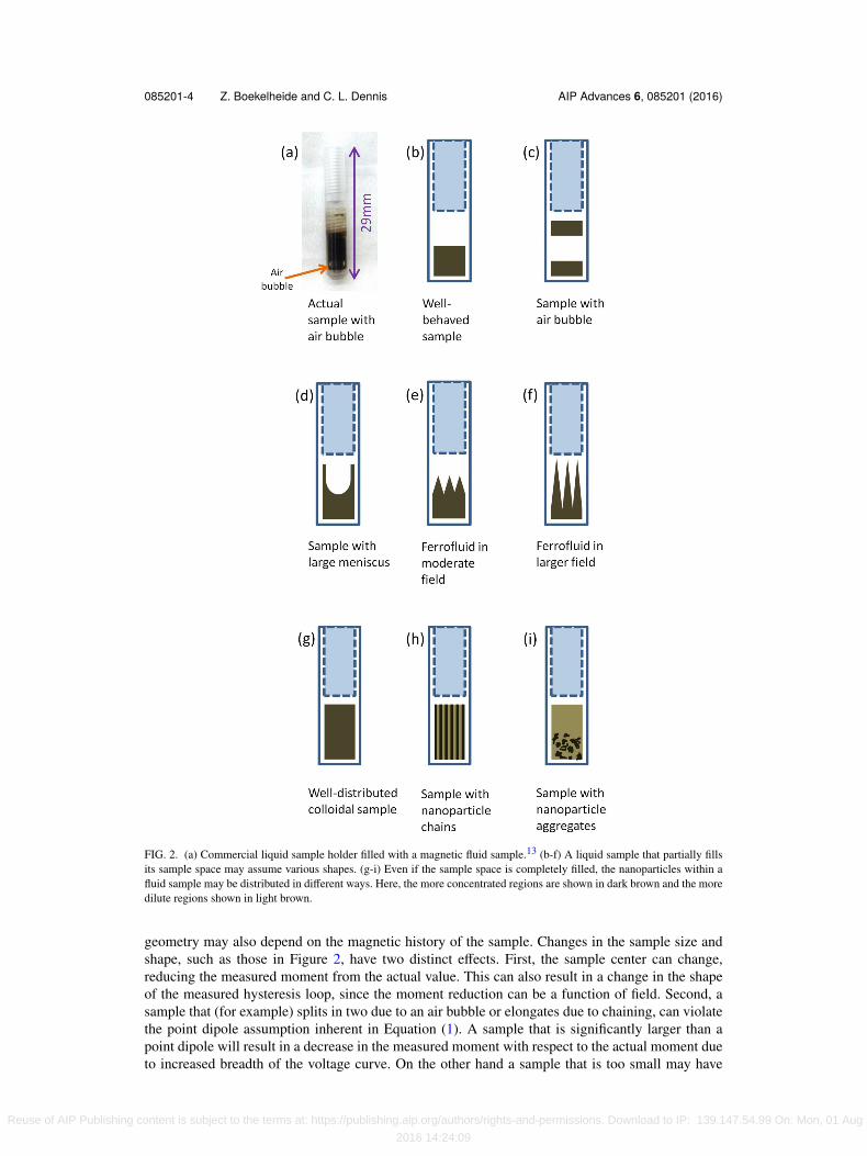
FIG. 2. (a) Commercial liquid sample holder filled with a magnetic fluid sample.13 (b-f) A liquid sample that partially fillsits sample space may assume various shapes. (g-i) Even if the sample space is completely filled, the nanoparticles within afluid sample may be distributed in different ways. Here, the more concentrated regions are shown in dark brown and the moredilute regions shown in light brown.

geometry may also depend on the magnetic history of the sample. Changes in the sample size andshape, such as those in Figure 2, have two distinct effects. First, the sample center can change,reducing the measured moment from the actual value. This can also result in a change in the shapeof the measured hysteresis loop, since the moment reduction can be a function of field. Second, asample that (for example) splits in two due to an air bubble or elongates due to chaining, can violatethe point dipole assumption inherent in Equation (1). A sample that is significantly larger than apoint dipole will result in a decrease in the measured moment with respect to the actual moment dueto increased breadth of the voltage curve. On the other hand a sample that is too small may have

Reuse of AIP Publishing content is subject to the terms at: https://publishing.aip.org/authors/rights-and-permissions. Download to IP: 139.147.54.99 On: Mon, 01 Aug

2016 14:24:09

085201-5 Z. Boekelheide and C. L. Dennis AIP Advances 6, 085201 (2016)

a low signal to noise ratio, obscuring the signal. For typical SQUID geometries, the point dipoleapproximation is valid for samples <5 mm, but the details are specific to each magnetometer’sgeometry.13,19

Figure 2(a) shows a photo of a commercially available liquid sample holder filled with a mag-netic fluid sample. It can be logistically difficult to fill such a cup-style sample holder completelywithout incorporating an air bubble. Figure 2(a) shows an air bubble at the bottom of the samplespace. Alternatively, it may be preferable to only partially fill the sample holder so that the sample is<5 mm in length. Either way, an air bubble in the sample space can cause significant issues becauseit allows movement of the sample within the sample space. For a partially filled sample holder,Figure 2(b) is the ideal scenario, and Figure 2(c)-2(f) shows different ways the sample can deviatefrom the single point dipole model, including an air bubble, a large meniscus, or normal instabilityin a ferrofluid. Normal instability in a ferrofluid causes a corrugated, spiked surface20,21 For thesecases, in addition to the sample shape changing, the center position is also changed from the idealcase shown in (b).

Even if no air bubble is incorporated into the sample space, the nanoparticles within a fluidsample may assume different shapes. For example, when a magnetic field is applied, nanoparticlescan form long chains in the direction of the field, creating regions of the sample which are moreor less concentrated. The nanoparticles may also aggregate, either spontaneously or in response toan applied field history; aggregates then tend to sink to the bottom. These scenarios are shown inFigure 2(g)-2(i).

B. SQUID measurement

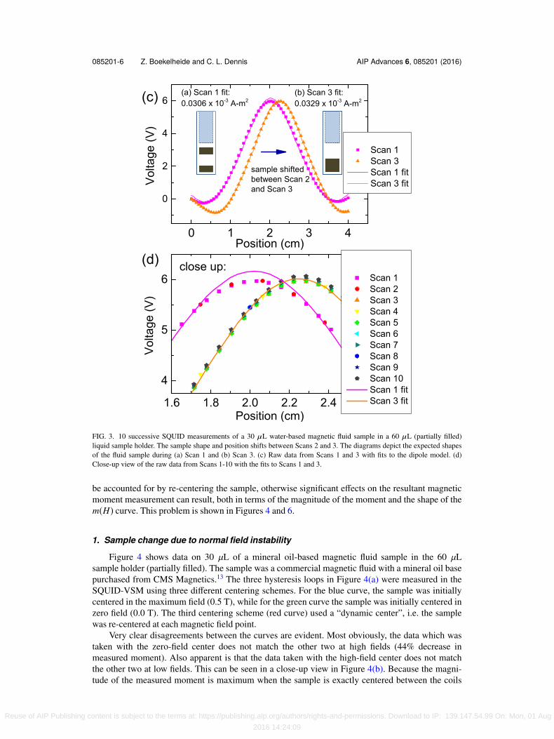
Figure 3 shows raw data from a SQUID measurement of a partially-filled sample holder, exper-imentally demonstrating both the shift in sample center position (peak position) and change in shape(peak width) that are a direct result of the dynamic physical nature of the sample. The sample was30 µL of a water-based magnetic fluid in a 60 µL (partially filled) liquid sample holder. The mag-netic fluid was a bionized nano-ferrite coated with a double dextran layer in a colloidal suspensionin H2O with solid content of 25 mg per mL.22 The initial sample shape approximated Figure 3(a)where some of the magnetic fluid adhered to the top of the sample holder space. After a series often scans at 300 K and 0.5 T, a change in the data between Scans 1-2 and Scans 3-10 is evident.When the sample was removed from the instrument immediately after the 10 scans, this change insample shape from Figure 3(a) to 3(b) could be seen visually. The raw data from Scans 1 and 3 areshown in Figure 3(c) and fit to the dipole model. The differences are as follows: first, the samplecenter position shifts by about 2.5 mm, about what would be expected for a shift from the shapeshown in Figure 3(a) to that in (b). Second, the width of the peak decreases, as the two point dipolescombine back into a single point dipole. A close up of the raw data from all ten scans is shown inFigure 3(d). Scan 1-2 overlap each other, and Scans 3-10 overlap each other; the significant changeoccurs between Scan 2 and Scan 3.

When analyzing the raw data from a SQUID measurement, the raw data is fit to the singledipole model (Equation (1)), shown as the solid lines in Figure 3(c)-3(d). The center position is a fitparameter, and therefore the exact center position does not have a significant effect on the resultantmagnetic moment unless the center is so far to one side that the full dipole curve is not capturedin the data. However, the deviation of the raw data from the dipole model fit in Scans 1 and 2means that the dipole assumption is not as accurate as in Scans 3-10. This deviation can be seenclearly in the close up view of the data in Figure 3(d). The magnetic moment obtained from thefit to Scan 1 (0.0306 × 10−3 A-m2) is 7% smaller than the moment obtained from the fit to Scan 3(0.0329 × 10−3 A-m2), where the sample shape better approximates the model assumptions of asingle point dipole.

C. SQUID VSM measurements

In contrast to the SQUID measurement where the sample center position is a fit parameter, in aSQUID VSM measurement, the sample center position is much more critical. A shift in center must

Reuse of AIP Publishing content is subject to the terms at: https://publishing.aip.org/authors/rights-and-permissions. Download to IP: 139.147.54.99 On: Mon, 01 Aug

2016 14:24:09

085201-6 Z. Boekelheide and C. L. Dennis AIP Advances 6, 085201 (2016)

FIG. 3. 10 successive SQUID measurements of a 30 µL water-based magnetic fluid sample in a 60 µL (partially filled)liquid sample holder. The sample shape and position shifts between Scans 2 and 3. The diagrams depict the expected shapesof the fluid sample during (a) Scan 1 and (b) Scan 3. (c) Raw data from Scans 1 and 3 with fits to the dipole model. (d)Close-up view of the raw data from Scans 1-10 with the fits to Scans 1 and 3.

be accounted for by re-centering the sample, otherwise significant effects on the resultant magneticmoment measurement can result, both in terms of the magnitude of the moment and the shape of them(H) curve. This problem is shown in Figures 4 and 6.

1. Sample change due to normal field instability

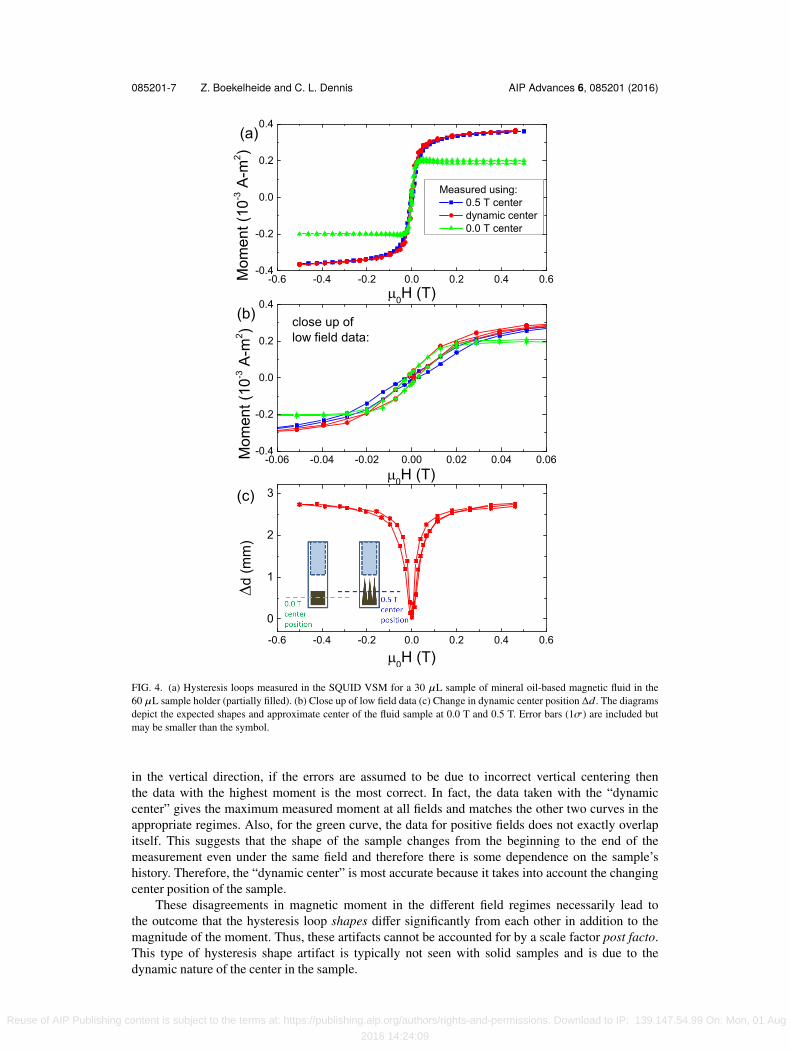
Figure 4 shows data on 30 µL of a mineral oil-based magnetic fluid sample in the 60 µLsample holder (partially filled). The sample was a commercial magnetic fluid with a mineral oil basepurchased from CMS Magnetics.13 The three hysteresis loops in Figure 4(a) were measured in theSQUID-VSM using three different centering schemes. For the blue curve, the sample was initiallycentered in the maximum field (0.5 T), while for the green curve the sample was initially centered inzero field (0.0 T). The third centering scheme (red curve) used a “dynamic center”, i.e. the samplewas re-centered at each magnetic field point.

Very clear disagreements between the curves are evident. Most obviously, the data which wastaken with the zero-field center does not match the other two at high fields (44% decrease inmeasured moment). Also apparent is that the data taken with the high-field center does not matchthe other two at low fields. This can be seen in a close-up view in Figure 4(b). Because the magni-tude of the measured moment is maximum when the sample is exactly centered between the coils

Reuse of AIP Publishing content is subject to the terms at: https://publishing.aip.org/authors/rights-and-permissions. Download to IP: 139.147.54.99 On: Mon, 01 Aug

2016 14:24:09

085201-7 Z. Boekelheide and C. L. Dennis AIP Advances 6, 085201 (2016)

FIG. 4. (a) Hysteresis loops measured in the SQUID VSM for a 30 µL sample of mineral oil-based magnetic fluid in the60 µL sample holder (partially filled). (b) Close up of low field data (c) Change in dynamic center position ∆d. The diagramsdepict the expected shapes and approximate center of the fluid sample at 0.0 T and 0.5 T. Error bars (1σ) are included butmay be smaller than the symbol.

in the vertical direction, if the errors are assumed to be due to incorrect vertical centering thenthe data with the highest moment is the most correct. In fact, the data taken with the “dynamiccenter” gives the maximum measured moment at all fields and matches the other two curves in theappropriate regimes. Also, for the green curve, the data for positive fields does not exactly overlapitself. This suggests that the shape of the sample changes from the beginning to the end of themeasurement even under the same field and therefore there is some dependence on the sample’shistory. Therefore, the “dynamic center” is most accurate because it takes into account the changingcenter position of the sample.

These disagreements in magnetic moment in the different field regimes necessarily lead tothe outcome that the hysteresis loop shapes differ significantly from each other in addition to themagnitude of the moment. Thus, these artifacts cannot be accounted for by a scale factor post facto.This type of hysteresis shape artifact is typically not seen with solid samples and is due to thedynamic nature of the center in the sample.

Reuse of AIP Publishing content is subject to the terms at: https://publishing.aip.org/authors/rights-and-permissions. Download to IP: 139.147.54.99 On: Mon, 01 Aug

2016 14:24:09

085201-8 Z. Boekelheide and C. L. Dennis AIP Advances 6, 085201 (2016)

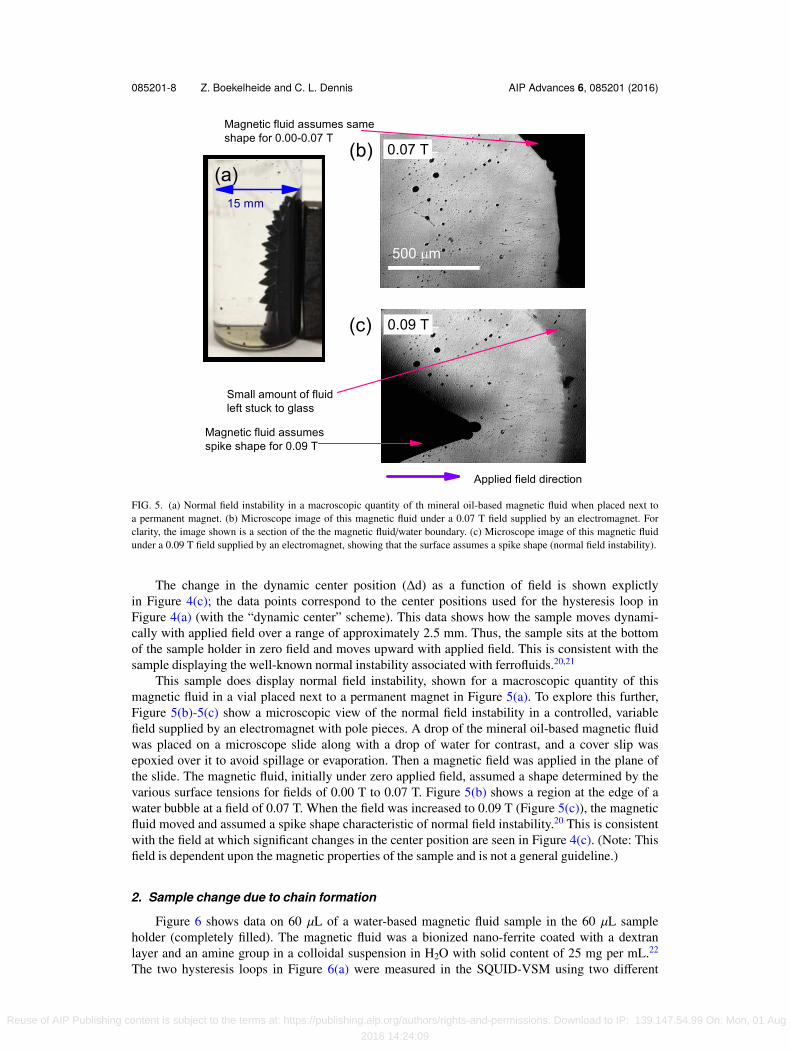
FIG. 5. (a) Normal field instability in a macroscopic quantity of th mineral oil-based magnetic fluid when placed next toa permanent magnet. (b) Microscope image of this magnetic fluid under a 0.07 T field supplied by an electromagnet. Forclarity, the image shown is a section of the the magnetic fluid/water boundary. (c) Microscope image of this magnetic fluidunder a 0.09 T field supplied by an electromagnet, showing that the surface assumes a spike shape (normal field instability).

The change in the dynamic center position (∆d) as a function of field is shown explictlyin Figure 4(c); the data points correspond to the center positions used for the hysteresis loop inFigure 4(a) (with the “dynamic center” scheme). This data shows how the sample moves dynami-cally with applied field over a range of approximately 2.5 mm. Thus, the sample sits at the bottomof the sample holder in zero field and moves upward with applied field. This is consistent with thesample displaying the well-known normal instability associated with ferrofluids.20,21

This sample does display normal field instability, shown for a macroscopic quantity of thismagnetic fluid in a vial placed next to a permanent magnet in Figure 5(a). To explore this further,Figure 5(b)-5(c) show a microscopic view of the normal field instability in a controlled, variablefield supplied by an electromagnet with pole pieces. A drop of the mineral oil-based magnetic fluidwas placed on a microscope slide along with a drop of water for contrast, and a cover slip wasepoxied over it to avoid spillage or evaporation. Then a magnetic field was applied in the plane ofthe slide. The magnetic fluid, initially under zero applied field, assumed a shape determined by thevarious surface tensions for fields of 0.00 T to 0.07 T. Figure 5(b) shows a region at the edge of awater bubble at a field of 0.07 T. When the field was increased to 0.09 T (Figure 5(c)), the magneticfluid moved and assumed a spike shape characteristic of normal field instability.20 This is consistentwith the field at which significant changes in the center position are seen in Figure 4(c). (Note: Thisfield is dependent upon the magnetic properties of the sample and is not a general guideline.)

2. Sample change due to chain formation

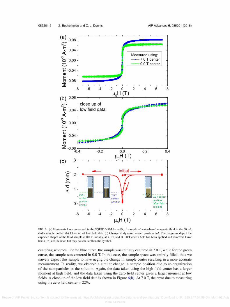
Figure 6 shows data on 60 µL of a water-based magnetic fluid sample in the 60 µL sampleholder (completely filled). The magnetic fluid was a bionized nano-ferrite coated with a dextranlayer and an amine group in a colloidal suspension in H2O with solid content of 25 mg per mL.22

The two hysteresis loops in Figure 6(a) were measured in the SQUID-VSM using two different

Reuse of AIP Publishing content is subject to the terms at: https://publishing.aip.org/authors/rights-and-permissions. Download to IP: 139.147.54.99 On: Mon, 01 Aug

2016 14:24:09

085201-9 Z. Boekelheide and C. L. Dennis AIP Advances 6, 085201 (2016)

FIG. 6. (a) Hysteresis loops measured in the SQUID VSM for a 60 µL sample of water-based magnetic fluid in the 60 µL(full) sample holder. (b) Close up of low field data (c) Change in dynamic center position ∆d. The diagrams depict theexpected shapes of the fluid sample at 0.0 T initially, at 7.0 T, and at 0.0 T after a field has been applied and removed. Errorbars (1σ) are included but may be smaller than the symbol.

centering schemes. For the blue curve, the sample was initially centered in 7.0 T, while for the greencurve, the sample was centered in 0.0 T. In this case, the sample space was entirely filled, thus wenaively expect this sample to have negligible change in sample center resulting in a more accuratemeasurement. In reality, we observe a similar change in sample position due to re-organizationof the nanoparticles in the solution. Again, the data taken using the high field center has a largermoment at high field, and the data taken using the zero field center gives a larger moment at lowfields. A close-up of the low field data is shown in Figure 6(b). At 7.0 T, the error due to measuringusing the zero field center is 22%.

Reuse of AIP Publishing content is subject to the terms at: https://publishing.aip.org/authors/rights-and-permissions. Download to IP: 139.147.54.99 On: Mon, 01 Aug

2016 14:24:09

085201-10 Z. Boekelheide and C. L. Dennis AIP Advances 6, 085201 (2016)

Figure 6(c) shows the center position measured at a few field values. The data suggests asimilar pattern as was seen in the mineral oil-based magnetic fluid. The center position varies overa range of approximately 2 mm, and changes rapidly at low field, flattening out at high fields. Onemajor difference is that the center data shows history dependence. Initially, the sample center doesnot change at all upon application of a field. It is only once a field is applied and then removed that achange in center is seen. This leads Figure 6(c) to be non-single-valued at low fields. (Note that themagnetic moment data shown in Figure 6(a) (green curve) was measured with the sample centeredin zero field after application and removal of a field.)

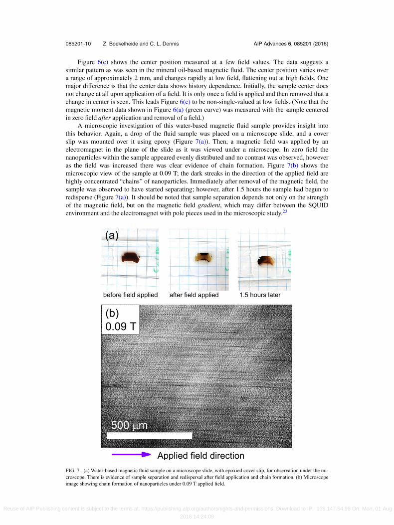
A microscopic investigation of this water-based magnetic fluid sample provides insight intothis behavior. Again, a drop of the fluid sample was placed on a microscope slide, and a coverslip was mounted over it using epoxy (Figure 7(a)). Then, a magnetic field was applied by anelectromagnet in the plane of the slide as it was viewed under a microscope. In zero field thenanoparticles within the sample appeared evenly distributed and no contrast was observed, howeveras the field was increased there was clear evidence of chain formation. Figure 7(b) shows themicroscopic view of the sample at 0.09 T; the dark streaks in the direction of the applied field arehighly concentrated “chains” of nanoparticles. Immediately after removal of the magnetic field, thesample was observed to have started separating; however, after 1.5 hours the sample had begun toredisperse (Figure 7(a)). It should be noted that sample separation depends not only on the strengthof the magnetic field, but on the magnetic field gradient, which may differ between the SQUIDenvironment and the electromagnet with pole pieces used in the microscopic study.23

FIG. 7. (a) Water-based magnetic fluid sample on a microscope slide, with epoxied cover slip, for observation under the mi-croscope. There is evidence of sample separation and redispersal after field application and chain formation. (b) Microscopeimage showing chain formation of nanoparticles under 0.09 T applied field.

Reuse of AIP Publishing content is subject to the terms at: https://publishing.aip.org/authors/rights-and-permissions. Download to IP: 139.147.54.99 On: Mon, 01 Aug

2016 14:24:09

085201-11 Z. Boekelheide and C. L. Dennis AIP Advances 6, 085201 (2016)

This chaining and separation behavior of this water-based magnetic fluid can explain themeasured center position of this sample. While well-dispersed to begin with, it is well-known thatmagnetic nanoparticles form chains upon application of a magnetic field in order to lower themagnetostatic energy of the system. When the field is removed, the chains are no longer the mostenergetically favorable; however, the nanoparticles do not necessarily quickly redisperse withoutshaking.24 Instead, the chains may separate into loose collections which settle to the bottom of thesample holder; this settling changes the sample center from its original position. Schematics of thisbehavior are shown as insets to Figure 6(c) alongside the center position data.

D. Immobilization of nanoparticles

Another potential measurement concern for magnetic fluids is immobilization of some nanopar-ticles in the sample when sealing the holder. For holders which close using screw threads, the screwthreads are sealed with epoxy to prevent the liquid portion of the sample from evaporating whilein an evacuated sample space. It is difficult to fill the sample space and seal the screw closurewithout incorporating some of the magnetic particles in the epoxy. Some nanoparticles immobilizedin epoxy this way can be seen in Figure 2(a).

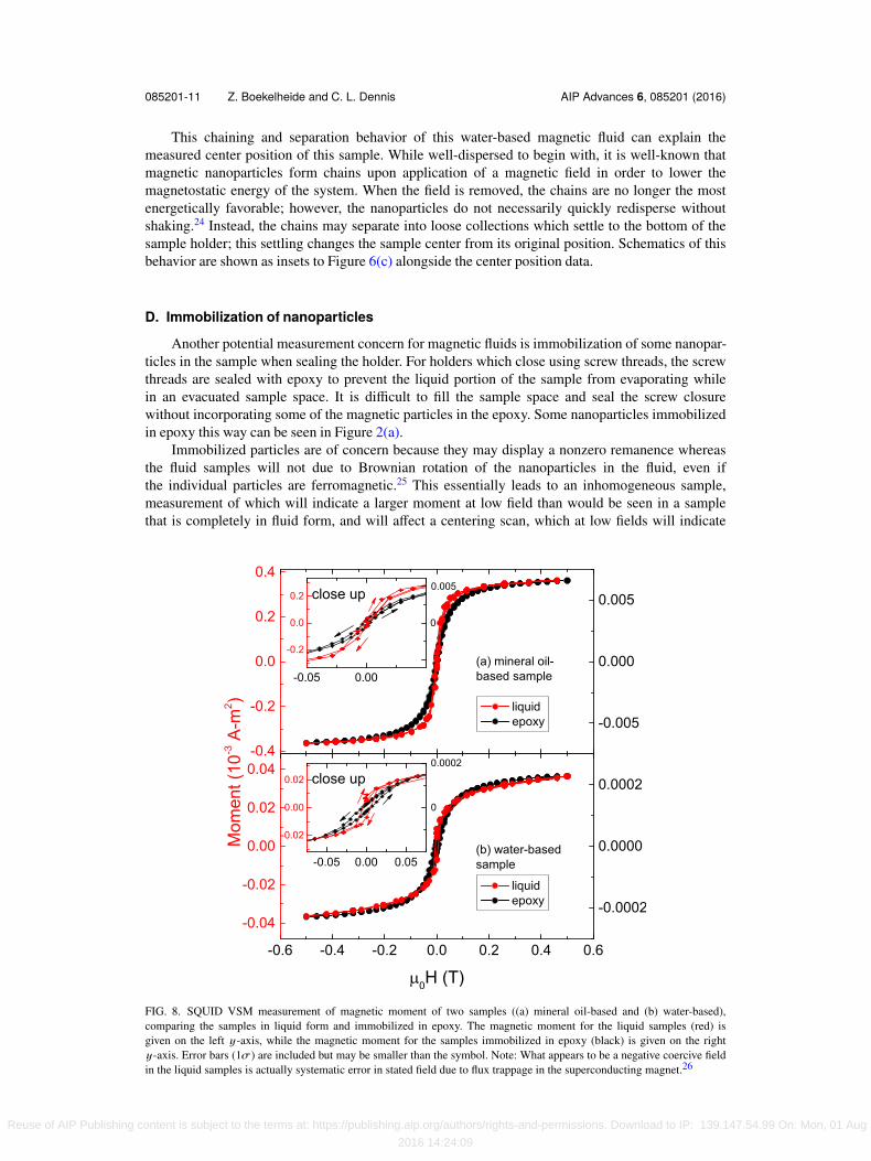
Immobilized particles are of concern because they may display a nonzero remanence whereasthe fluid samples will not due to Brownian rotation of the nanoparticles in the fluid, even ifthe individual particles are ferromagnetic.25 This essentially leads to an inhomogeneous sample,measurement of which will indicate a larger moment at low field than would be seen in a samplethat is completely in fluid form, and will affect a centering scan, which at low fields will indicate

FIG. 8. SQUID VSM measurement of magnetic moment of two samples ((a) mineral oil-based and (b) water-based),comparing the samples in liquid form and immobilized in epoxy. The magnetic moment for the liquid samples (red) isgiven on the left y-axis, while the magnetic moment for the samples immobilized in epoxy (black) is given on the righty-axis. Error bars (1σ) are included but may be smaller than the symbol. Note: What appears to be a negative coercive fieldin the liquid samples is actually systematic error in stated field due to flux trappage in the superconducting magnet.26

Reuse of AIP Publishing content is subject to the terms at: https://publishing.aip.org/authors/rights-and-permissions. Download to IP: 139.147.54.99 On: Mon, 01 Aug

2016 14:24:09

085201-12 Z. Boekelheide and C. L. Dennis AIP Advances 6, 085201 (2016)

that the center position is at the center of the immobilized particles only, ignoring the fluid portionof the sample. This would cause errors due to centering shifts as described previously.

Figure 8 compares hysteresis loops for the two magnetic fluids, in fluid form and immobilizedin epoxy. The nanoparticles in both samples are magnetically soft enough that the potential sourcesof error described due to nonzero remanence are not significant. Essentially, the coercive field of theimmobilized nanoparticles is smaller than the systematic error on the magnetic field measurementdue to flux trappage in the superconducting magnet,26 therefore the potential sources of error dueto immobilized nanoparticles are not relevant for these particular samples. However, researchersworking with magnetic fluids containing particles with large coercivity should be aware of thispotential source of error.

IV. SUMMARY

Figures 3, 4, and 6 demonstrate artifacts in magnetic measurements of fluid samples. Arti-facts arise from: (a) Change of sample center position during measurement, (b) change of sampleshape during measurement, and (c) change in distribution of magnetic particles within sample fluid.Potential for error exists due to nanoparticles immobilized in the sample holder sealing process(e.g., epoxy), resulting in non-zero remanence due solely to immobilized particles. Awareness ofthese artifacts among the growing magnetic fluid community will improve the accuracy of reportedmeasurements.

Our recommendations for accurate magnetic measurement of fluid samples include: (a) pre-vent large scale sample motion by minimizing air bubbles in sample container, (b) for measurementmethods which rely on a predetermined center position, recenter before each measurement, or (c) usemeasurement methods which account for changes in sample center, (d) ensure sample size is withinthe recommended limits for the measurement system, (e) avoid immobilizing nanoparticles in samplesealing (e.g., epoxy), and (f) monitor raw data for violations in point dipole approximation.

ACKNOWLEDGMENTS

The authors thank Cordula Gruettner of micromod Partikeltechnologie GmbH for the water-based magnetic fluid (BNF) samples.

1 Y. T. Choi and N. M. Werely, “Vibration control of a landing gear system featuring electrorheological/magnetorheologicalfluids,” Journal of Aircraft 40, 432 (2003).

2 P. J. Blennerhassett, F. Lin, and P. J. Stiles, “Heat transfer through strongly magnetized ferrofluids,” Proc. R. Soc. Lond. A433, 165 (1991).

3 Y.-X. J. Wang, “Superparamagnetic iron oxide based MRI contrast agents: Current status of clinical application,” Quant.Imaging Med. Surg. 1, 35 (2011).

4 J. Weizenecker, B. Gleich, J. Rahmer, H. Dahnke, and J. Borgert, “Three-dimensional real-time in vivo magnetic particleimaging,” Phys. Med. Biol. 54, L1 (2009).

5 C. L. Dennis, A. J. Jackson, J. A. Borchers, P. J. Hoopes, R. Strawbridge, A. R. Foreman, J. van Lierop, C. Gruttner,and R. Ivkov, “Nearly complete regression of tumors via collective behavior of magnetic nanoparticles in hyperthermia,”Nanotechnology 20, 395103 (2009).

6 M. Bonini, S. Lenz, R. Giorgi, and P. Baglioni, “Nanomagnetic sponges for the cleaning of works of art,” Langmuir 23,8681 (2007).

7 H. Mamiya and B. Jeyadevan, “Hyperthermic effects of dissipative structures of magnetic nanoparticles in large alternatingmagnetic fields,” Sci. Rep. 1, 157 (2011).

8 S. G. Sherman, D. A. Paley, and N. M. Wereley, “Parallel simulation of transient magnetorheological direct shear flowsusing millions of particles,” IEEE Transactions on Magnetics 48, 3517 (2012).

9 A. P. Philipse and D. Maas, “Magnetic colloids from magnetotactic bacteria: chain formation and colloid stability,” Langmuir18, 9977 (2002).

10 S. Foner, “Versatile and sensitive vibrating-sample magnetometer,” Review of Scientific Instruments 30, 548 (1959).11 M. McElfresh, “Fundamentals of magnetism and magnetic measurements featuring Quantum Design’s Magnetic Property

measurement System,” Tech. Rep. (Quantum Design, 1994).12 W. Burgei, M. J. Pechan, and H. Jaeger, “A simple vibrating sample magnetometer for use in a materials physics course,”

American Journal of Physics 71, 825 (2003).13 Certain commercial equipment, instruments, or materials are identified in this paper to foster understanding. Such

identification does not imply recommendation or endorsement by the National Institute of Standards and Technology, nordoes it imply that the materials or equipment identified are necessarily the best available for the purpose.

Reuse of AIP Publishing content is subject to the terms at: https://publishing.aip.org/authors/rights-and-permissions. Download to IP: 139.147.54.99 On: Mon, 01 Aug

2016 14:24:09

085201-13 Z. Boekelheide and C. L. Dennis AIP Advances 6, 085201 (2016)

14 J. Xu, K. Mahajan, W. Xue, J. Winter, M. Zborowski, and J. Chalmers, “Simultaneous, single particle, magnetization andsize measurements of micron sized, magnetic particles,” Journal of Magnetism and Magnetic Materials 324, 4189 (2012).

15 A. L. Balk, C. Hangarter, S. M. Stavis, and J. Unguris, “Magnetometry of single ferromagnetic nanoparticles using magneto-optical indicator films with spatial amplification,” Applied Physics Letters 106, 112402 (2015).

16 “MPMS Application Note 1014-213 Subtracting the Sample Holder Background from Dilute Samples,” Quantum Design(2002).

17 Magnetic Property Measurement System SQUID-VSM User’s Manual, Quantum Design, San Diego, CA, 13th ed. (2010).18 “SQUID VSM Application Note 1500-010 Rev. A0 Accuracy of the Reported Moment: axial and radial sample positioning

error,” Quantum Design (2010).19 “SQUID VSM Application Note 1500-015 Rev. A0 Accuracy of the Reported Moment: Sample Shape Effects,” Quantum

Design (2010).20 M. D. Cowley and R. E. Rosensweig, “The interfacial stability of a ferromagnetic fluid,” J. Fluid Mech. 30, 671 (1967).21 A. R. Zakinyan and L. S. Mkrtchyan, “Instability of the ferrofluid layer on a magnetizable substrate in a perpendicular

magnetic field,” Magnetohydrodynamics 48, 615 (2012).22 C. Grüttner, K. Müller, J. Teller, F. Westphal, A. Foreman, and R. Ivkov, “Synthesis and antibody conjugation of mag-

netic nanoparticles with improved specific power absorption rates for alternating magnetic field cancer therapy,” Journal ofMagnetism and Magnetic Materials 311, 181 (2007).

23 The magnetic field gradient next to a permanent magnet is larger than that of a solenoid producing the magnetic field in amagnetometer. However, a solenoid is necessarily finite and therefore also produces a gradient.

24 G. Cheng, C. L. Dennis, R. D. Shull, and A. R. Hight Walker, “Influence of the Colloidal Environment on the MagneticBehavior of Cobalt Nanoparticles,” Langmuir 23, 11740 (2007).

25 N. A. Clark, “Ferromagnetic ferrofluids,” Nature 504, 229 (2013).26 “MPMS Application Note 1014-208 Remnant Fields in MPMS Superconducting Magnets,” Quantum Design (2002).

Reuse of AIP Publishing content is subject to the terms at: https://publishing.aip.org/authors/rights-and-permissions. Download to IP: 139.147.54.99 On: Mon, 01 Aug

2016 14:24:09