Article Post-Print The following article is a “post-print” of an article accepted for publication in an

Elsevier journal.

Castillo, P., Mahalec, V. Improved continuous-time model for gasoline

blend scheduling, Computers & Chemical Engineering,, 84 627-646 (2016)

The post-print is not the final version of the article. It is the unformatted version

which has been accepted for publication after peer review, but before it has

gone through the editing and formatting process with the publisher. Therefore,

there may be minor editorial differences between this version and the final

version.

The final, official version of the article can be downloaded from the journal’s

website via this DOI link when it becomes available (subscription or purchase

may be required):

doi:10.1016/j.compchemeng.2015.08.003

This post-print has been archived on the author’s personal website

(macc.mcmaster.ca) in compliance with the National Sciences and Engineering

Research Council (NSERC) policy on open access and in compliance with

Elsevier’s academic sharing policies.

This post-print is released with a Creative Commons Attribution Non-

Commercial No Derivatives License.

Date Archived: May 27, 2016

1

Improved Continuous-Time Model for Gasoline Blend Scheduling

Pedro A. Castillo-Castillo, Vladimir Mahalec*

Department of Chemical Engineering, McMaster University, 1280 Main St. West, Hamilton,

ON, L8S 4L8, Canada

* Corresponding author. Tel.: +1 905 525 9140 ext. 26386. E-mail address:

mahalec@mcmaster.ca

Keywords: Gasoline blend scheduling; continuous-time model; reduced number of discrete

variables; nonlinear blending models.

Abstract

This work introduces a reduced-size continuous-time model for scheduling of gasoline

blends. Previously published model has been modified by i) introducing new model features

(penalty for deliveries in order to reduce sending material from different product tanks to the same

order, product and blender-dependent minimum setup times, maximum delivery rate from

component tanks, threshold volume for each blend), ii) by reducing the number of integer

variables, and iii) by adding lower bounds on the blend and switching costs, which significantly

improve convergence. Nonlinearities are introduced by ethyl RT-70 equations for octane blending.

Medium-size linear problems (two blenders, more than 20 orders, 5 products) are solved to

optimality within one or two minutes. Previously unsolved large scale blending problems (more

than 35 orders, 5 product, 2 or 3 blenders) have also been solved to less than 0.5% optimality gap.

1. Introduction

Scheduling of a production plant involves making decisions to determine what and when

the tasks must be executed, and in which processing units, in order to fulfill product demands along

a given time horizon while meeting product specifications, storage and capac-ity constraints, and

raw materials availability. Complex plants, such as oil-refineries, can have multiple processes,

large number of raw materials with different quality properties, several intermediate and final

products, and intricate pipeline and storage systems that make scheduling a difficult decision

process. Determining the optimal production schedule can reduce operational costs, increase profit

margins, and avoid deviations from environmental constraints (Harjunkoski et al., 2014).

Mathematical programming is the most common approach to handle scheduling problems and

several mixed-integer programming models and techniques have been developed and applied to

solve scheduling problems in chemical production plants during the past three decades (Velez and

2

Maravelias, 2015). However, due to the combinatorial nature of the problem, scheduling remains

a research intensive and challenging area. Scheduling models can be divided into those employed

for batch processes and those utilized for continuous processes. Batch plant models do not require

explicit material balances since material batches neither merge nor split and they can be tracked

along the processing stages. On the other hand, material balances are required to be included in

continuous plant models since material batches are allowed to merge and/or split. Another type of

classification of scheduling models is based on the representation of time:

a) Discrete-time models – The scheduling horizon is divided into time periods of known

duration. Recently, Velez and Maravelias (2015) described a methodology to

incorporate non-uniform time grids into a discrete-time model (i.e. the number of time

periods is different for each process or unit).

b) Continuous-time models – The scheduling horizon is partitioned into several time slots

whose duration is not known in advance and it is calculated during the optimization

procedure. One global time grid can be used (i.e. the variables representing the time

slots are the same for all units), as well as unit-specific time grids (i.e. the variables

representing the time slots are different for each unit). Fixed time periods can be

incorporated as well, and time slots are assigned to them, i.e. time slots start and end

within such periods (e.g. Mendez et al., 2006; Neiro et al., 2014). The boundaries of

these fixed time periods can be delineated by intermediate product due dates or calendar

days.

In general, only one task can occur in a given processing unit during one time period or

time slot. Each time representation has its advantages and disadvantages. Discrete-time models are

much simpler to write than corresponding continuous-time models, but they usually require large

number of time periods which increases their size (i.e. number of equations, continuous and

discrete variables, etc.). Continuous-time models may require less number of discrete variables,

but sometimes they could be less tight than corresponding discrete-time models (Joly and Pinto,

2003). Floudas and Lin (2004), Sundaramoorthy and Maravelias (2011), Maravelias (2012), and

Harjunkoskiet al. (2014) present more thorough reviews of discrete- and continuous-time

scheduling models.

In this work, we present a continuous-time model for gasoline blend scheduling (a

continuous process), which is an extensive modification of the previously published scheduling

model by Li and Karimi (2011). This new version of the model adds additional operational

constraints (minimization of deliveries of the same product from different tanks, limit on the

maximum rate of delivery from component tanks, minimum volumetric size of a blend run, and

product-dependent setup times), includes lower bounds on the objective function, contains

equations to transform some binary variables into 0–1 continuous variables, and reduces the total

number of binary variables in the model by making use of the demand information.

The paper is structured as follows: Section 2 is a brief overview of the prior work in this

area, while Section 3 presents the problem statement. Section 4 describes the new version of the

3

full-space blend scheduling model. Section 5 describes the examples used in this work. Section 6

presents computational results and it shows that the proposed lower bounds added to the full-space

model significantly reduce solution times. As summarized in Section 7, the proposed new version

of the full-space model can be solved much faster than the previously published model (Li and

Karimi, 2011); however, large-scale problems still cannot be solved to proven optimality in

reasonable time (e.g. <3 h).

2. Scheduling of Gasoline Blending Operations

The gasoline blending process is a common example found in the literature on planning

and scheduling optimization problems since gasoline is one of the main products of an oil refinery,

both in quantity and profit margins (Mendez et al., 2006; Li and Karimi, 2011). Moreover, the

problem is easy to understand and its corresponding mathematical model can be formulated as an

LP, NLP, MILP, or MINLP, depending of the assumptions, scope, and the required accuracy.

Jia and Ierapetritou (2003) constructed a continuous-time MILP model to schedule gasoline

blending operations and its distribution. The model includes multipurpose product tanks (swing

tanks), minimum run length requirements, and employs fixed recipes in order to maintain the

linearity of the model.

Mendez et al. (2006) developed both a discrete- and continuous-time MILP model to

schedule blending operations. They incorporate the off-line blending problem (i.e. recipe

optimization) into the scheduling model, and they handle nonlinear blending rules through an

iterative method. However, the distribution problem is not considered and not many logistic

constraints are included (e.g. multipurpose tanks, non-identical blenders, minimum blend size,

etc.).

Li et al. (2010) presented a continuous-time slot-based MILP model that uses process slots;

i.e. a common global time grid for all units. This model includes blend recipe optimization, parallel

non-identical blenders, multipurpose tanks, inventory constraints, blender capacity constraints,

delivery scheduling for the demand orders, and other constraints found in industrial practice. Li

and Karimi (2011) replaced process slots with unit slots (i.e. each unit has its specific time grid)

and expanded the model by Li et al. (2010) to include blender setup times and simultaneous

receipt/delivery by product tanks. Their execution times and final solutions were better than those

from Li et al. (2010), but the large-scale case studies (e.g. 2–3 blenders, 5 products, 9 components,

9 quality properties, 11 product tanks, 35–45 orders, and a planning horizon of 8 days) still used

all the allocated CPU time (46,800–118,800 s, depending on the problem) and the optimality gaps

were not reported.

Kolodziej et al. (2013) formulated a discrete-time MINLP model for the pooling problem

including inventory, flow, and quality constraints. The nonlinearities arise from the initial

inventory of the blending tanks at each time period as a blend component. Since the quality

properties of these initial inventories are not known after the first time period, the quality

4

constraints involve bilinear nonconvex terms. In addition to one heuristic solution procedure, they

proposed two different algorithms to solve this MINLP model to global optimality using a radix-

based discretization technique which discretizes one variable in the bilinear terms found in the

model in order to obtain MILP relaxations. Their largest case study has 8 tanks, 4 time periods

(each 1 day long), and 2 quality properties. Their execution times range from a few seconds to

2840 s, depending on the problem instance.

3. Problem Statement

In this work, we address the gasoline blend scheduling problem stated as follows:

Given:

1. A short term scheduling horizon [0, H].

2. A set of components, their properties, initial inventories, costs, and flow rates along the

horizon (i.e., supply profile).

3. A set of products (i.e. gasoline grades) with prescribed minimum and maximum quality

specifications, their initial inventories and corresponding initial quality.

4. A set of delivery orders for each product along the horizon (i.e., demand profile).

5. The maximum blending capacity of each blender.

6. A set of storage tanks and their minimum and maximum capacities.

7. Nonlinear or linear blending model.

The objective is to determine:

1. The blend recipes (i.e. the volume fractions of the blend components in each product) for

each blend that will be made along the horizon.

2. The blenders that each component tank should feed over time, and the corresponding feed

rates.

3. The products that each blender should produce over time, and their production rates.

4. The products that each product tank should receive over time, from which blender, and at

what flow rates.

5. The orders that each product tank should deliver over time, their amounts and delivery

rates.

6. The inventory profiles of component and product tanks.

7. Swing tanks product allocation along the horizon.

Minimizing:

1. Total cost which consists of the total cost of the blended materials plus the switching costs

(i.e. number of blend runs, number of tanks delivering the same order, and product

transitions in the swing tanks) and the demurrage costs.

Subject to:

1. If a blender is to produce a product, it must blend at least a minimum amount.

5

2. A blender can produce at most one product at any time. Once it begins blending, it must

operate for some minimum time before it can switch to another product.

3. A blender requires a minimum setup time during a product changeover

4. A blender can feed at most one product tank at any time (industrial practice).

5. Product tanks can only store one product at any time.

Assuming:

1. Flow rate profile of each component from the upstream process is piecewise constant.

2. Component quality profile is piecewise constant.

3. Perfect mixing occurs in each blender.

4. There is only one tank for a given blend component.

5. There is no minimum flow restriction from component tanks to blenders.

6. Only product tanks defined as swing tanks can change its product service (i.e. change from

storing one product to store another).

7. Changeover times between products are negligible for swing tanks.

8. For each blender, changeover times between product blending are product-dependent but

sequence-independent.

9. Each order involves only one product (one original order involving different products can

be broken into orders of each specific product).

10. Each order is completed during the scheduling horizon.

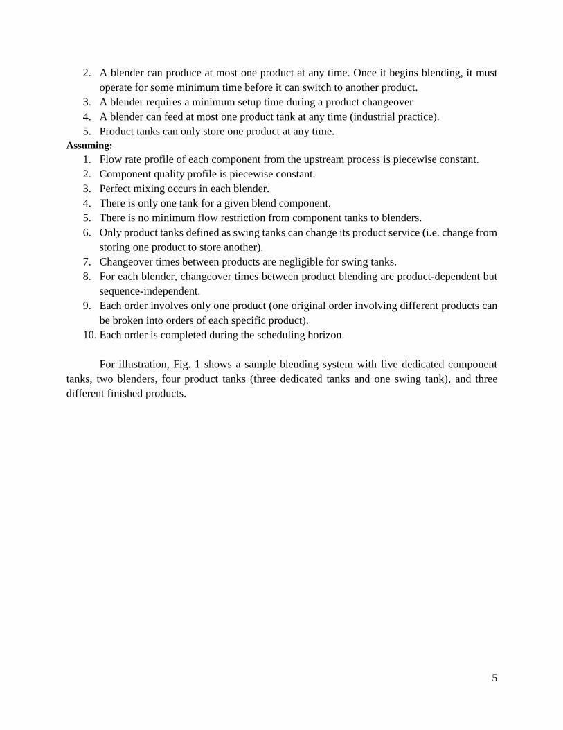
For illustration, Fig. 1 shows a sample blending system with five dedicated component

tanks, two blenders, four product tanks (three dedicated tanks and one swing tank), and three

different finished products.

6

Fig. 1. Sample blending system.

4. Continuous-Time Full-Space Blend Scheduling Model

In this section, we present the continuous-time full-space blend scheduling model used in

this work. This model is based on the one developed by Li and Karimi (2011), which was selected

because it considers most of the key operational features of a blending system. We describe the

differences between the two versions of this blend scheduling model. The notation used in this

paper is not identical to the one presented by Li and Karimi (2011) since this model will be used

in future work in combination with our previously published discrete-time models (Castillo and

Mahalec, 2014a, 2014b). We denote as (LK-#) the equation number # presented by Li and Karimi

(2011). We only present the equations for the case when there are different supply flow rates and

quality profiles of blend components along the horizon (the multi-period model or MPM as

denoted by Li and Karimi, 2011) since the case when they are constant can be handled by these

equations as well.

One third of the equations are new, while two thirds are parts that are contained in the Li

and Karimi model. The equations that are identical or equivalent to those presented by Li and

Karimi (2011) are Eqs. (6)–(9), (11)–(18), (22)–(27), (29)–(35), (44)–(49), (54)–(60),(62)–

(72), (77)–(82), (87)–(101), (103)–(108). The equations added or modified and presented in this

7

work are Eqs. (1)–(5), (10), (19)–(21),(28), (36)–(43), (50)–(53), (61), (73)–(76), (83)–(86), (102),

(109)–(113).

Three sets of modifications have been made to Li and Karimi (2011) model. Modification

set #1 adds the following operational and model features:

a) Minimization of deliveries of the same order from different product tanks (Eq. (3)).

b) Minimization of number of blend runs by penalizing only the start of a blend run

(Eqs. (3), (20), (21)).

c) Addition of slack variables which ensure that a numerical solution is obtained, even

if the problem is infeasible (Eqs. (1), (5), (61), (73),(74)).

d) Minimum volume to be blended during a blend run (Eqs. (50)–(53)).

e) Product- and blender-dependent minimum setup times (Eqs. (36)–(43)).

f) Limit on the maximum delivery rate from the blend component tanks (Eqs. (75),

(76), (83)–(86)).

Modification set #2 reduces the number of binary variables (Eqs. (19), (28), (102), and

construction of refined sets for the delivery constraints).

Modification set #3 incorporates lower bounds on the blend cost and switching costs (Eqs.

(109) and (110)).

Although these modifications significantly improve the solution times required by the full-

space model, it can still take more than 3 h to solve to proven optimality medium and large-size

problems.

4.1. Time slots sets

From the original set of all time slots N0 = {n | n = 0, 1, . . ., N − 1, N}, three different

subsets are constructed: set N1 does not include the first slot (in this case, n = 0), set N2 does not

include the last slot (in this case, n = N), and set N3 does not include neither the first or last slot.

Note that the time slots are “unit slots”, which means that each unit has its specific time grid. From

here on, the terms time slot and unit slot will be used interchangeably.

4.2. Time periods and delivery slots sets

Binary variable z(j,o,n) is equal to 1 if product tank j is sending material to order o during

slot n, and 0 otherwise. Set JO = {(j,o) | tank j may deliver order o} is composed of the pairs (j,o)

found in the intersection of set JP = {(j,p) | tank j can store product p} and set PO = {(p,o) | product

p constitutes order o}. Writing the corresponding order delivery equations for all (j,o)JO and all

nN1 generates unnecessary instantiations of binary variable z(j,o,n), which does not need to be

introduced before the start time of the delivery window of the corresponding order, i.e. )(oTO start

order

; and in most cases, the orders are likely to be completed before or just a few hours after the end

of the delivery window, i.e. )(oTO end

order . Based on the demand information, and the allocation of

8

time slots to fixed time periods along the scheduling horizon, it is possible to define set ON =

{(o,n) | order o may be delivered during time slot n} and set JON = {(j,o,n) | tank j may deliver

order o during time slot n}. Set JON is constituted by the triplets (j,o,n) from the intersection of

sets JO and ON. If set ON contains less number of elements than {(o,n) | oO, nN1}, then the

number of instantiations of variable z(j,o,n) is reduced when using set JON in the model instead

of {(j,o,n) | (j,o) JO, n N1}.

In the MPM approach of Li and Karimi (2011), fixed time periods are defined by different

supply flowrates or quality profiles of blend components; however, more time periods can be

added, even when the supply flowrates and qualities of blend components are constant along the

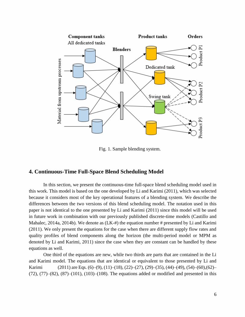
scheduling horizon. In this work, set M = {1, …, m, …, M – 1, M} denotes the fixed time periods

and set MN = {(m, n) | time slot n is assigned to time period m} represents the allocation of time

slots to fixed time periods. If (m,n) MN, then slot n must end within period m (see Fig. 2).

Boundaries of the time periods of set M must include the times where changes are expected in the

supply flowrates or qualities of the blend components. As mentioned before, more time periods

can be added. However, this may increase the number of time slots required to solve the problem

to optimality and therefore is only recommended if their addition decreases the total number of

discrete variables in the model. For simplicity, in this work we only use the fixed time periods

delineated by different supply flowrates of blend components.

Set ON is constructed in the following way: If a portion of the time delivery window of

order o lies within time period m, then order o may be delivered during the slots assigned to such

time period. For the examples presented in this work, set JON reduces 30 to 58% of the total

number of discrete variables in the model.

Fig. 2. Time slots and fixed time periods.

9

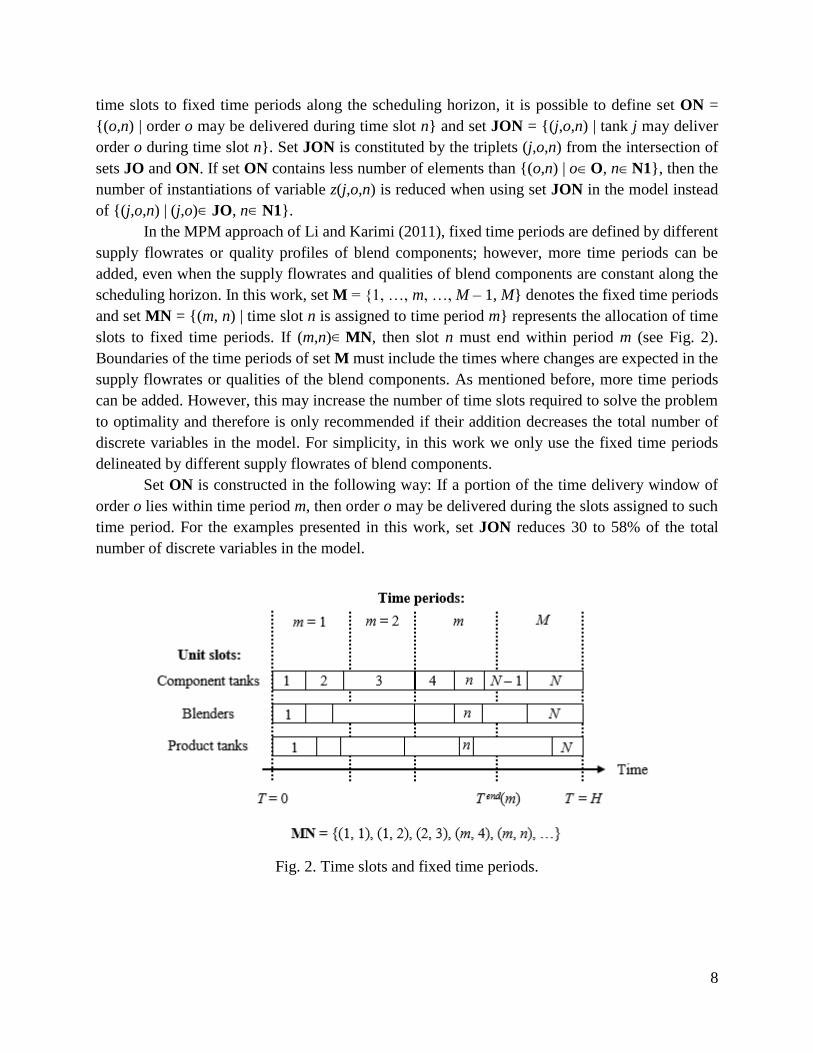
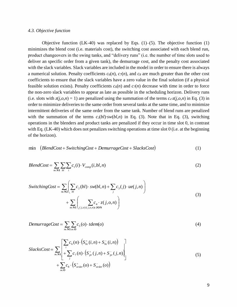
4.3. Objective function

Objective function (LK-40) was replaced by Eqs. (1)–(5). The objective function (1)

minimizes the blend cost (i.e. materials cost), the switching cost associated with each blend run,

product changeovers in the swing tanks, and “delivery runs” (i.e. the number of time slots used to

deliver an specific order from a given tank), the demurrage cost, and the penalty cost associated

with the slack variables. Slack variables are included in the model in order to ensure there is always

a numerical solution. Penalty coefficients c6(n), c7(n), and c8 are much greater than the other cost

coefficients to ensure that the slack variables have a zero value in the final solution (if a physical

feasible solution exists). Penalty coefficients c6(n) and c7(n) decrease with time in order to force

the non-zero slack variables to appear as late as possible in the scheduling horizon. Delivery runs

(i.e. slots with z(j,o,n) = 1) are penalized using the summation of the terms c4·z(j,o,n) in Eq. (3) in

order to minimize deliveries to the same order from several tanks at the same time, and to minimize

intermittent deliveries of the same order from the same tank. Number of blend runs are penalized

with the summation of the terms c2(bl)·sw(bl,n) in Eq. (3). Note that in Eq. (3), switching

operations in the blenders and product tanks are penalized if they occur in time slot 0, in contrast

with Eq. (LK-40) which does not penalizes switching operations at time slot 0 (i.e. at the beginning

of the horizon).

SlacksCostostDemurrageCostSwitchingCBlendCost min (1)

N1n bl i

comp nbliVicBlendCost ),,()(1 (2)

N1 JON

N2

n nojoj

n jbl

nojzc

njuejcnblswblcostSwitchingC

),,(:),(

4

32

),,(

),()(),()(

(3)

N1 On o

otdemocostDemurrageC )()(5 (4)

O

N1

o

orderorder

n

j

prpr

i

bcbc

oSoSc

njSnjSnc

niSniSnc

SlacksCost

)()(

),(),()(

),(),()(

8

7

6

(5)

10

4.4. Time slots definition

Variable Tunit(unit_index,n) represents the end time of the unit slot n. These times are

bounded by the beginning and end of the associated time period, i.e. Tstart(m) ≤ Tbc(i,n), Tpr(j,n),

Tb(bl,n) ≤ Tend(m), for all m, i, j, bl, and n:(m,n) MN. Eqs. (6)–(8) state that the end time of a unit

slot must be equal to or greater than the end time of the previous unit slot. The initial unit slots are

constrained to be equal to 0 by equation (9), and the last unit slots are forced to be equal to the

length of the scheduling horizon by equation (10).

)1,(),( niTniT bcbc N1 ni, (6)

)1,(),( njTnjT prpr N1 nj, (7)

)1,(),( nblTnblT bb N1 nbl, (8)

0),(),(),( nblTnjTniT bprbc 0,,, nblji (9)

HnblTnjTniT bprbc ),(),(),( Nnblji ,,, (10)

4.5. Binary and 0-1 continuous variables

Binary variable v(j,bl,n) is 1 if product tank j is receiving material from blender bl in slot

n, and 0 otherwise. 0-1 continuous variable x(p,bl,n) is 1 if product p is being produced by blender

bl in slot n, and 0 otherwise. 0-1 continuous variable w(bl,n) represents the status of blender bl

during slot n and it is equal to 0 (if the blender is running) or 1 (if the blender is idle). A blender

can only process one product and can only feed one product tank in each slot, see Eq. (11) and

(12).

1),,(),(),(:

BPblpp

nblpxnblw N1 nbl, (11)

1),,(),(),(:

BJbljj

nbljvnblw N1 nbl, (12)

Binary variable u(j,p,n) is 1 if product tank j is holding product p during slot n, and 0

otherwise. Eq. (13) constrains a product tank to hold not more than one specific product type in

each slot. If a blender produces product p in slot n, there must at least one product tank j holding

that particular product type in that slot, and there must exist a physical connection between the

11

blender and such product tank, as stated by Eq. (14) and (15). Li et al. (2010) showed that Eq. (14)

and (15) make x(p,bl,n) a 0-1 continuous variable.

1),,(),(:

JPpjp

npju N1 nj, (13)

1),,(),,(),,( nbljvnpjunblpx

N1BJJPBP nbljpjblp ,),(,),(,),( (14)

1),,(),,(),,( nbljvnpjunblpx

N1BJJPBP nbljpjblp ,),(,),(,),( (15)

0-1 continuous variable xe(bl,n) represents a state transition in blender bl at the end of slot

n, i.e. a transition from being running to being idle, or vice versa, see Eqs. (16)–(19).

)1,,(),,(),( nblpxnblpxnblxe N2BP nblp ,),( (16)

),,()1,,(),( nblpxnblpxnblxe N2BP nblp ,),( (17)

)1,,(),,(2),( nblpxnblpxnblxe N2BP nblp ,),( (18)

)1,(),(2),( nblwnblwnblxe N2 nbl, (19)

Continuous variable sw(bl,n) represents the start of a blend run in blender bl at the

beginning of slot n+1. sw(bl,n) is constrained to have values between 0 and 1 by Eq. (20) and (21),

but since it is penalized in the objective function (1), it behaves like a 0-1 continuous variable. Li

and Karimi (2011) did not use a variable similar to sw(bl,n) because they penalize corresponding

variable xe(bl,n). However, when including non-zero setup times, it is possible that a blender

requires an idle slot between blend runs; we do not want to penalize the transition from running to

idle, and then from idle to running (a double penalty). By using variable sw(bl,n), we avoid a

double penalty for a single blend run.

)1,(),(),( nblwnblxenblsw N2 nbl, (20)

2/),(),(),( nblwnblxenblsw N2 nbl, (21)

Continuous variable ue(j,n) represents a product transition in swing tank j at the end of slot

n if it is equal to 1. This variable is defined by Eq. (22) and (23). ue(j,n) is bounded to be equal to

or less than 1 (i.e. ue(j,n) ≤ 1, j, n).

12

)1,,(),,(),( npjunpjunjue N2JP npj ,),( (22)

),,()1,,(),( npjunpjunjue N2JP npj ,),( (23)

Eq. (24) states that a product tank j cannot deliver order o if it does not hold the

corresponding product p. Using equation (25), a product tank cannot receive and deliver product

at the same time.

),,(),,( npjunojz POJONN1 ),(:,),,(:),(, oppnojojn (24)

1),,(),,( nojznbljv BJJONN1 ),(:,),,(:),(, bljblnojojn (25)

0-1 continuous variable y(i,bl,n) is equal to 1 if blend component i is being used in blender

bl during slot n, and 0 otherwise. Eq. (26) ensures that if a blender is idle, it cannot receive material.

If a blender is running, it must receive at least one blend component, as stated by Eq. (27).

Including Eq. (28) in the model makes y(i,bl,n) a 0-1 continuous variable. However, Eq. (28)

synchronizes most of the component tank slots with the blender slots, and hence, the number of

time slots required to solve the problem to optimality may increase. This has been observed

particularly in small-scale problems (see Section 6). Nevertheless, computed solutions are still of

the same quality and, for medium- and large-scale problems, number of binary variables does not

increase and the execution times are shorter than when not including Eq. (28) and using y(i,bl,n)

as a binary variable. If a minimum pumping rate from the tanks to the blenders is imposed

(constraint that it is not considered in this work), Eq. (28) should not be included in the model and

y(i,bl,n) must be defined as a binary variable.

1),,(),( nbliynblw N1 nbli ,, (26)

1),,(),( i

nbliynblw N1 nbl, (27)

BP),(:

),,(),,(blpp

nblpxnbliy N1 nbli ,, (28)

Therefore, only three binary variables are required by this model: u(j,p,n), v(j,bl,n) and

z(j,o,n).

13

4.6. Blending - Time constraints

A blender must process a product at least for a minimum amount of time given by

parameter ),(min blpctblend , see Eqs. (29)–(35). Continuous variables tblend(bl,n) and ctblend(bl,n)

represent the blending time during slot n and the cumulative blending time (since the start of the

current blend run) at the beginning of slot n, for blender bl, respectively. Eq. (29) constrains

tblend(bl,n) to be equal to or less than the blender slot duration, while Eq. (30) forces the equality

unless the blender is idle or is at the last slot of a blend run. Eq. (31) forces tblend(bl,n) to be equal

to zero if the blender is idle.

)1,(),(),( nblTnblTnblt bbblend N1 nbl, (29)

),(),()1,(),(),( nblxenblwHnblTnblTnblt bbblend

N1 nbl, (30)

),(1),( nblwHnbltblend N1 nbl, (31)

Eq. (32) restricts ctblend(bl,n) to be equal to or less than the cumulative time at the end of

slot n – 1 plus the blending time during slot n. If a blender changes its state, the cumulative time

is reset to zero by Eq. (33). A blender that is running during slot n can only change its state in n+1

if the cumulative blending time up to n is greater than the minimum specified, see Eq. (34). Eq.

(35) is a version of Eq. (34) specified for the last slot of the horizon.

),()1,(),( nbltnblctnblct blendblendblend N1 nbl, (32)

),(1),( nblxeHnblctblend N1 nbl, (33)

),(1)(),,(),(),()1,(),(:

min nblxeblRLnblpxblpctnbltnblct blend

BPblpp

blendblendblend

N3 nbl, (34)

BPblpp

blendblendblend nblpxblpctnbltnblct),(:

min ),,(),(),()1,( Nnbl , (35)

Where ),(max)( min

),(:blpctblRL blend

blppblend

BP bl .

Before a new blend run, a blender requires an idle time at least equal to the setup time given

by parameter ),(min blpcitblend , see Eqs. (36)–(43). Variable itblend(bl,n) represents the idle time of

14

blender bl during slot n, and variable citblend(bl,n) is the cumulative idle time (since the end of the

last blend run) of blender bl at the beginning of slot n. Eq. (36) constrains itblend(bl,n) to be less than

the blender slot duration minus the blending time, and Eq. (37) forces itblend(bl,n) to be equal to

zero unless the blender is idle or is at the last slot of a blend run. Eq. (38) constraints itblend(bl,n) to

be equal to zero during the last time slot unless the blender is idle.

)1,(),(),(),( nblTnblTnbltnblit bbblendblend N1 nbl, (36)

),(),(),( nblwnblxeHnblitblend N1 nbl, (37)

),(),( nblwHnblitblend Nnbl , (38)

The cumulative idle time at slot n is equal to or less than the idle time from slot n – 1 plus

the idle time during slot n, see Eq. (39). When a blender is running, the cumulative idle time

citblend(bl,n) is reset to zero by Eq. (40). The cumulative idle time must be at least the current idle

time at slot n, this is imposed by Eq. (41) and (42). An idle blender can only change its state after

the minimum idle time has been completed, see Eq. (43).

),()1,(),( nblitnblcitnblcit blendblendblend N1 nbl, (39)

),(),(),( nblwnblxeHnblcitblend N1 nbl, (40)

),(),( nblitnblcit blendblend N1 nbl, (41)

),(),(),( nblwHnblitnblcit blendblend N1 nbl, (42)

)1,,(1)()1,(),(),(),( min nblpxblILnblwnblxeblpcitnblcit blendblendblend

N2BP nblp ,),( (43)

Where ),(max)( min

),(:blpcitblIL blend

blppblend

BP bl .

4.7. Blending - Material balance equations

Volume processed by a blender is the same as the volume coming from the component

tanks and the volume transferred to the product tanks, see Eq. (44) and (45). Only one product tank

can receive product within a time slot, as Eq. (12) and (46) enforce. The volume from each

15

component to the blender is limited by the pumping rate of each component tank or the blender

capacity, see Eq. (47).

i

compblend nbliVnblV ),,(),( N1 nbl, (44)

BJ),(:

),,(),(bljj

transblend nbljVnblV N1 nbl, (45)

),,()(),,( max nbljvHblFnbljV blendtrans N1BJ nblj ,),( (46)

),,(),(),,( nbliyHblinbliVcomp N1 nbli ,, (47)

Where )(),,(min),( maxmax blFbliFbli blendcomp bli, .

4.8. Blending – Volume threshold constraints

The volume produced by a blender must be between its minimum and maximum

production rates, according to Eq. (48) and (49).

),()(),( min nbltblFnblV blendblendblend N1 nbl, (48)

),()(),( max nbltblFnblV blendblendblend N1 nbl, (49)

A blend run must end after a minimum volume given by parameter ),(min blpCVblend has been

produced, see Eqs. (50)–(53). Variable CVblend(bl,n) is the cumulative blended volume (since the

start of the current blend run) at the beginning of slot n in blender bl. CVblend(bl,n) is constrained

by Eq. (50) to be equal to or less than the cumulative volume from slot n – 1 plus the volume

blended during slot n. CVblend(bl,n) is reset to zero by Eq. (51) if a blender changes its state. Eq.

(52) and (53) permit a blender to finish a blend run only after the minimum volume has been

produced.

),()1,(),( nblVnblCVnblCV blendblendblend N1 nbl, (50)

),(1)(),( max nblxeHblFnblCV blendblend N1 nbl, (51)

16

),(1)(),,(),(),()1,(),(:

min nblxeblVLnblpxblpCVnblVnblCV blend

blpp

blendblendblend BP

N3 nbl, (52)

BP),(:

min ),,(),(),()1,(blpp

blendblendblend nblpxblpCVnblVnblCV Nnbl , (53)

Where ),(max)( min

),(:blpCVblVL blend

blppblend

BP bl .

4.9. Blending – Composition constraints

Eqs. (54) and (55) ensure that the amount of blend components per unit of product are

within the minimum and maximum composition limits, respectively.

),,(1)(),(),(),(),(),,( minminmin nblpxipirHblinblVpirnbliV blendcomp

N1BP nblpi ,),(, (54)

),,(1),()(),(),(),(),,( maxmaxmax nblpxpiriHblinblVpirnbliV blendcomp

N1BP nblpi ,),(, (55)

Where ),(min)( minmin pirip

i and ),(max)( maxmax pirip

i .

4.10. Blending - Quality balance equations

One of the assumptions in the Problem Statement (Section 3) is a piecewise constant

component quality profile. Parameter Qbc(i,e,θ) represents the value of quality property e for blend

component i during quality profile θ. Set QN = {(θ, n)} indicates which time slots correspond to

each quality profile. The quality properties that blend linearly on a volumetric basis are constrained

by Eqs. (56) and (57) to ensure that the final product quality is within the minimum and maximum

specifications, respectively. Eqs. (58) and (59) are analogous for the quality properties that blend

linearly on a weight basis.

),,(1)(),()(

),(),(),,(),,(

minminmax

min

nblpxeepQHblF

nblVepQeiQnbliV

prblend

blendpr

i

bccomp

QNN1BPEV ),(:,,),(, nnblpe (56)

17

),,(1),()()(

),(),(),,(),,(

maxmaxmax

max

nblpxepQeHblF

nblVepQeiQnbliV

prblend

blendpr

i

bccomp

QNN1BPEV ),(:,,),(, nnblpe (57)

Where ),(min)( minmin epQe prp

e , and ),(max)( maxmax epQe prp

e .

),,(1)(),()(

),(),,(),(),(),,(),,(

maxminminmax

min

nblpxeepQHblF

inbliVepQieiQnbliV

prblend

i

comppr

i

bccomp

QNN1BPEW ),(:,,),(, nnblpe (58)

),,(1),()()(

),(),,(),(),(),,(),,(

maxmaxmaxmax

max

nblpxepQeHblF

inbliVepQieiQnbliV

prblend

i

comppr

i

bccomp

QNN1BPEW ),(:,,),(, nnblpe (59)

Where ),(max,

max

ii

.

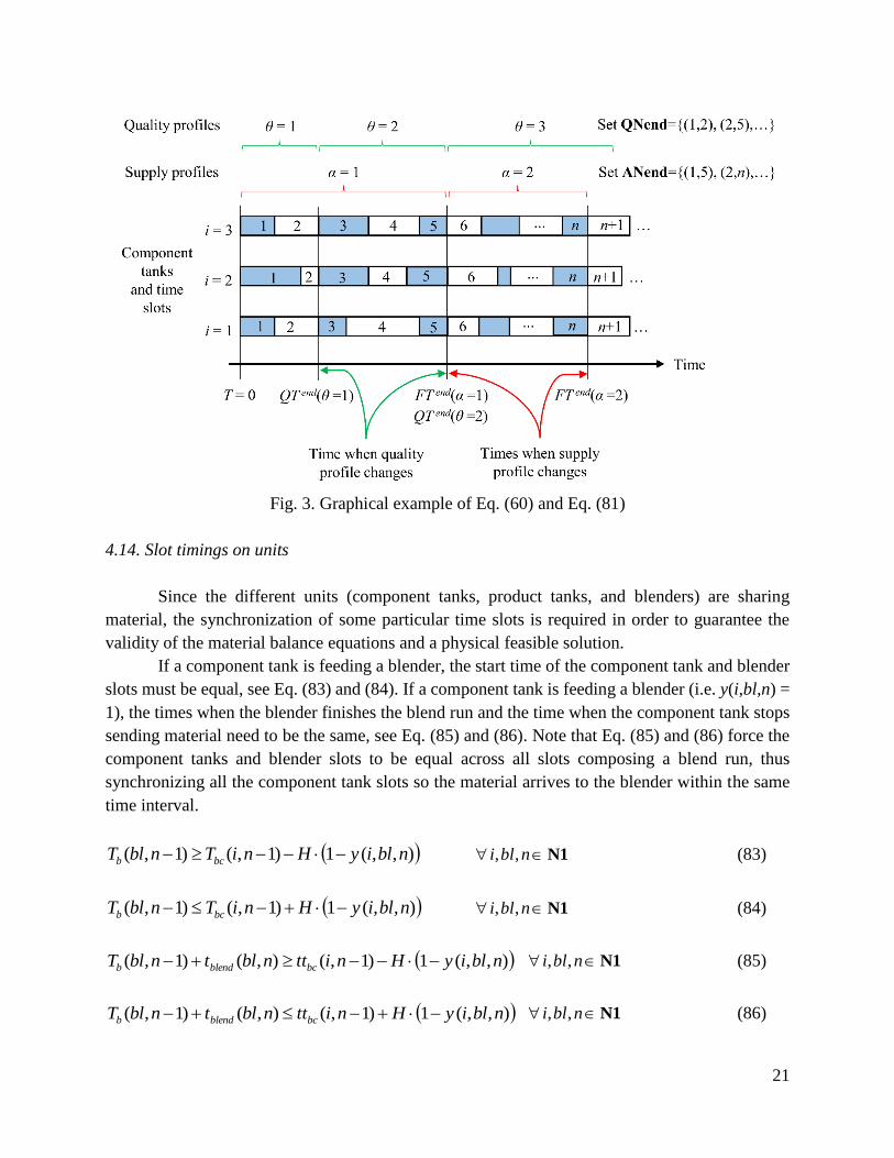
Equation (60) constrains the last component tank slots with a given quality profile to

coincide with the time when such quality profile ends. This equation assumes that the first quality

profile starts at time equal to 0. Eq. (60) is required to avoid using material of a given quality that

is not available anymore, or not available yet. See Fig. 3 for an example of Eq. (60).

)(),( end

bcbc QTniT QNend ),(:,, nni (60)

4.11. Order delivery constraints

Li and Karimi (2011) used fixed delivery rates for each order (i.e. if a tank is sending

product to meet order o, it must do it at the rate specified a priori for order o). In our model, if the

delivery rate for each order is not known, we let the delivery rate vary between maximum and

minimum rates, denoted as )(max oDorder and )(min oDorder

, respectively. A fixed delivery rate is obtained by

making both of these parameters equal.

Eq. (61) constrains the amount of volume delivered from the product tanks to the

shipping/lifting ports, plus positive and negative slack variables, is equal to the demand. By Eq.

(62), the total delivery rate of tank j must be smaller than its maximum possible. The delivery rate

18

of product tank j to satisfy order o must be smaller than the maximum delivery rate of such tank,

and the maximum and minimum delivery rates specified for order o, according to Eq. (63), (64)

and (65), respectively. If tank j is delivering order o during slot n, then binary variable z(j,o,n) is

equal to 1 by Eq. (66).

)()()(),,(),,(:

oDemandoSoSnojDV orderorder

n nojj

pr

N1 JON

Oo (61)

)1,(),()(),,( max

),,(:

njTnjTjDnojDV prprpr

nojo

pr

JON

N1 nj, (62)

),,()(),,( max nojtdjDnojDV orderprpr JONN1 ),,(:),(, nojojn (63)

),,()(),,( max nojtdoDnojDV orderorderpr JONN1 ),,(:),(, nojojn (64)

),,()(),,( min nojtdoDnojDV orderorderpr JONN1 ),,(:),(, nojojn (65)

),,()(),,( nojzoDemandnojDVpr JONN1 ),,(:),(, nojojn (66)

4.12. Order delivery – Time constraints

Continuous variable tdorder(j,o,n) represents the time used during slot n to deliver order o

from tank j, and it must be equal to or less than the length of such time slot, see Eq. (67). Note that

Li and Karimi (2011) did not require this variable since they use a term of the form (delivered

volume)/(fixed delivery rate) to calculate it.

The start time to deliver order o from product tank j during slot n, i.e. tsorder(j,o,n), must be

equal to or greater than the start time of such product tank slot (i.e. the end time of the previous

slot), see Eq. (68). The end time to deliver order o within slot n must be equal to or less than the

end time of that slot, as stated by Eq. (69). Eq. (70) constrains tsorder(j,o,n) to be equal to or greater

than the beginning of the corresponding time delivery window.

)1,(),(),,( njTnjTnojtd prprorder JONN1 ),,(:),(, nojojn (67)

)1,(),,( njTnojts prorder JONN1 ),,(:),(, nojojn (68)

),(),,(),,( njTnojtdnojts prorderorder JONN1 ),,(:),(, nojojn (69)

19

),,()(),,( nojzoTOnojts start

orderorder JONN1 ),,(:),(, nojojn (70)

Eq. (71) computes the time outside the delivery window required to complete order o

(which is used in Eq. (4) to calculate the demurrage cost). All orders must be completed within the

scheduling horizon, as stated by Eq. (72).

),,(1)(),,(),,()( nojzHoTOnojtdnojtsotdem end

orderorderorder

JONN1 ),,(:),(, nojojn (71)

)()( oTOHotdem end

order Oo (72)

4.13. Inventory balance

The volume in product tank j at the end of slot n, i.e. Vpr(j,n), is equal to the volume at the

end of slot n – 1 plus the volume transferred from the blenders minus the volume sent to the

shipping/lifting ports, plus the corresponding positive and negative slack variables, see Eq. (73).

One of the assumptions in Section 3 is a piecewise constant component supply profile.

Variable Fbc(i,α) represents the flow rate of blend component i during supply profile α. Set AN =

{(α, n)} indicates which time slots correspond to each supply profile. The volume in component

tank i at the end of slot n, i.e. Vbc(i,n), is equal to the volume at the end of slot n – 1 plus the volume

received during that interval minus the volume send to the blenders, plus the corresponding

positive and negative slack variables, see Eq. (74).

),(),(),,(

),,()1,(),(

),,(:

),(:

njSnjSnojDV

nbljVnjVnjV

prpr

nojo

pr

bljbl

transprpr

JON

BJ

N1 nj, (73)

),(),(),,(

)1,(),(),()1,(),(),(:

niSniSnbliV

niTniTiFniVniV

bcbc

bl

comp

n

bcbcbcbcbc

AN

N1 ni, (74)

The total volume sent from tank i to all blenders is limited by the maximum pumping rate

of such tank or the maximum total production rate (Eq. (75)). Continuous variable ttbc(i,n) indicates

the time when a component tank stops sending materials to the blenders. Eq. (76) ensures that such

variable is within the corresponding time slot.

)1,(),()(),,( niTnittinbliV bcbc

bl

comp N1 ni, (75)

20

),(),()1,( niTnittniT bcbcbc N1 ni, (76)

Where iblFbliFibl

blend

bl

comp

)(,),(min)( maxmax .

Eqs. (77) and (78) force the inventory levels to be within the minimum and maximum limits

at the end of the unit slot, and Eqs. (79) and (80) at the moment when the tank stops sending

material to the blenders.

)(),()( maxmin jVnjVjV prprpr N1 nj,

(77)

)(),()( maxmin iVniViV bcbcbc N1 ni, (78)

bl

comp

n

bcbcbc

bcbc

nbliVniTnittiF

niViV

),,()1,(),(),(

)1,()(

),(:

min

AN

N1 ni, (79)

bl

comp

n

bcbcbc

bcbc

nbliVniTnittiF

niViV

),,()1,(),(),(

)1,()(

),(:

max

AN

N1 ni, (80)

Equation (81) constrains the last component tank slots with a given supply profile to

coincide with the time when such supply profile ends. This equation assumes that the first supply

profile starts at time equal to 0. Eq. (81) is required to avoid using material not available yet, as

well as to prevent disregarding material. See Fig. 3 for an example of Eq. (81).

)(),( end

bcbc FTniT ANend ),(:,, nni (81)

A swing tank can only change its service if it is empty, as required by Eq. (82).

),(1)(),( max njuejVnjV prpr N2 nj, (82)

21

Fig. 3. Graphical example of Eq. (60) and Eq. (81)

4.14. Slot timings on units

Since the different units (component tanks, product tanks, and blenders) are sharing

material, the synchronization of some particular time slots is required in order to guarantee the

validity of the material balance equations and a physical feasible solution.

If a component tank is feeding a blender, the start time of the component tank and blender

slots must be equal, see Eq. (83) and (84). If a component tank is feeding a blender (i.e. y(i,bl,n) =

1), the times when the blender finishes the blend run and the time when the component tank stops

sending material need to be the same, see Eq. (85) and (86). Note that Eq. (85) and (86) force the

component tanks and blender slots to be equal across all slots composing a blend run, thus

synchronizing all the component tank slots so the material arrives to the blender within the same

time interval.

),,(1)1,()1,( nbliyHniTnblT bcb N1 nbli ,, (83)

),,(1)1,()1,( nbliyHniTnblT bcb N1 nbli ,, (84)

),,(1)1,(),()1,( nbliyHnittnbltnblT bcblendb N1 nbli ,, (85)

),,(1)1,(),()1,( nbliyHnittnbltnblT bcblendb N1 nbli ,, (86)

22

When considering that product tanks cannot receive and deliver material at the same time,

it is enough to ensure that the start of the product tank slot precedes the start of the blender slot,

and that the end of the product tank slot succeeds the end of the blend run, see Eq. (87) and (88).

)1,,(1)1,(),()1,( nbljvHnbltnblTnjT blendbpr

N2BJ nblj ,),( (87)

)1,,(1),(),( nbljvHnblTnjT bpr N2BJ nblj ,),( (88)

4.15. Initial conditions

For the first time slot, variables x(p,bl,n), v(j,bl,n), u(j,p,n), w(bl,n), Vbc(i,n), Vpr(j,n),

ctblend(bl,n), citblend(bl,n), itblend(bl,n), and CVblend(bl,n), are set equal to their initial values (Eqs. (89)–

(98)).

),(),,( blpxnblpx ini 0,),( nblp BP (89)

),(),,( bljvnbljv ini 0,),( nblj BJ (90)

),(),,( pjunpju ini 0,),( npj JP (91)

)(),( blwnblw ini 0, nbl (92)

)(),( iVniV ini

bcbc 0, ni (93)

)(),( jVnjV ini

prpr 0, nj (94)

)(),( blctnblct ini

blendblend 0, nbl (95)

)(),( blcitnblcit ini

blendblend 0, nbl (96)

)(),( blitnblit ini

blendblend 0, nbl (97)

)(),( blCVnblCV ini

blendblend 0, nbl (98)

4.16. Simultaneous receipt/delivery by product tanks

If the product tanks are allowed to receive and deliver material at the same time, Eq. (25)

is omitted from the model and Eqs. (99)–(107) are added. 0-1 continuous variable ze(j,o,n) is equal

to 1 if tank j starts or stops delivering material to order o at the end of product tank slot n, see Eqs.

(99)–(101).

)1,,(),,(),,( nojznojznojze JONN2 ),,(:),(, nojojn (99)

),,()1,,(),,( nojznojznojze JONN2 ),,(:),(, nojojn (100)

23

)1,,(),,(2),,( nojznojznojze JONN2 ),,(:),(, nojojn (101)

)1,,(),,(),,( nojznojznojze JONN2 ),,(:),(, nojojn (102)

Eqs. (67), (68), (103), and (104) force the start and end times of a product tank slot to be

equal to the delivery times used in each slot.

),,(),,(1),(),,(),,( nojzenojzHnjTnojtdnojts prorderorder

JONN1 ),,(:),(, nojojn (103)

),,()1,,(1),()1,,( nojzenojzHnjTnojts prorder

JONN2 ),,(:),(, nojojn (104)

Eqs. (105)–(108) match the start and end times of a blender slot with those of a delivery

run from the product tank receiving material from such blender.

),,(),,(2)1,(),,( nojznbljvHnblTnojts border

BJJONN1 ),(:,),,(:),(, bljblnojojn (105)

),,(),,(2)1,(),,( nojznbljvHnblTnojts border

BJJONN1 ),(:,),,(:),(, bljblnojojn (106)

),,(),,(2),()1,(

),,(),,(

nojznbljvHnbltnblT

nojtdnojts

blendb

orderorder

BJJONN1 ),(:,),,(:),(, bljblnojojn (107)

),,(),,(2),()1,(

),,(),,(

nojznbljvHnbltnblT

nojtdnojts

blendb

orderorder

BJJONN1 ),(:,),,(:),(, bljblnojojn (108)

4.17. Lower bounds for the materials and switching costs

An estimation of lower bounds can be determined for the materials and switching costs. A

lower bound for the materials cost can be computed by formulating and solving an aggregate

optimization model minimizing the materials cost subject to the components availability, the

maximum blending capacity and inventory constraints, using a single period for the entire horizon

24

or a multi-period model using the inventory pinch concept to delineate the time period boundaries

(e.g. Castillo et al., 2013; Castillo & Mahalec, 2014a, 2014b). The volumes of components from

the aggregate solution are used in Eq. (109).

i

aggcomp iVicBlendCost )()( ,1 (109)

A lower bound for the switching cost can be estimated by Eq. (110). swexp is the expected

minimum number of blend runs, which is determined as follows: (i) for a given product, if the

result of (initial inventory) – (total demand during the horizon) – (minimum inventory limit) is

negative, that product must be blended during the scheduling horizon at least once, (ii) after

determining which different products are required, subtract those that are being blended at the

beginning of the horizon. ueexp is the expected minimum number of product changeovers in the

swing tanks, which can be estimated as the number of different products required to be blended

that are not initially stored by any product tank. Finally, at least one delivery run is expected for

each order. The notation ||set|| indicates the number of elements in the set.

||||)(min)(min 4exp3exp2 O

cuejcswblcostSwitchingC

jbl (110)

4.18. Nonlinear blending models

Eqs. (111)–(113) correspond to nonlinear blending models and quality specifications.

Inclusion of Eq. (111) will result in a MINLP scheduling model. The nonlinear equations used in

this work are presented in section 4.2.

),,(),,(),,,(),,( eiQnblVnbliVfneblQ bcblendcomppr

QNN1ENL ),(:,,, nnebl (111)

),,(),(),,( min nblpxepQneblQ prpr N1BPENL nblpe ,),(, (112)

),,(1)(),(),,( maxmax nblpxeepQneblQ prpr N1BPENL nblpe ,),(, (113)

4.19. Scheduling adjustment (reducing blending rate variations)

The presented continuous-time scheduling model does not assume fixed blending rates

(although this can be easily incorporated into the model if desired by setting )()( maxmin blFblF blendblend

) and it does not compute them directly (in order to avoid nonconvex nonlinear terms). Therefore,

if a blend run spans several time slots, it is possible that the blending rates vary across the slots. In

25

order to reduce such variations, average blending rates are computed based on the solution from

the full-space model and, with the production and delivery sequence fixed, the full-space model is

resolved minimizing the difference between the average and actual blending rates.

4.20. Versions of the full-space model

The following notation is used. “L” stands for linear blending rules, “N” for nonlinear

blending equations, “SimRD” means that simultaneous receipt/delivery by product tanks is

permitted, and “NoSimRD” indicates that simultaneous receipt/delivery by product tanks is not

allowed. Different operational scenarios can be constructed as follows:

(i) No simultaneous receipt/delivery by product tanks, based on linear models, model

L-NoSimRD is defined by Eqs. (1)–(98), (109), and (110).

(ii) Simultaneous receipt/delivery by product tanks, based on linear models, model

L-SimRD is described by Eqs. (1)–(24), and (26)–(110).

(iii) No simultaneous receipt/delivery by product tanks, based on non-linear models,

model N-NoSimRD is defined by Eqs. (1)–(98), and (109)–(113).

(iv) Simultaneous receipt/delivery by product tanks, based on non-linear models,

model N-SimRD is defined by Eqs. (1)–(24), and (26)–(113).

4.21. Nonlinear blending equations

In this work, we only consider the research octane number (RON) and the motor octane

number (MON) as the properties to blend nonlinearly following the ethyl RT-70 models (Singh et

al., 2000; Healey et al., 1959). Therefore, set ENL = {‘RON’, ‘MON’}. In the ethyl RT-70 models,

RON and MON are functions of the blend components sensitivity (i.e. sens(i) = Qbc(i,’RON’) –

Qbc(i,’MON’)), and olefins (‘OLF’) and aromatics (‘ARO’) content. Eq. (111) is substituted by

Eqs. (111-a)–(111-l). The model parameter values used by Singh et al. (2000) are: a1 = 0.03224,

a2 = 0.00101, a3 = 0, a4 = 0.04450, a5 = 0.00081, and a6 = – 0.0645.

),(),,(),,( nblVnblirnbliV blendcomp N1 nbli ,, (111-a)

i

bc

RON

avg eiQnblirnblr ),,(),,(),( QNN1 ),(:,,,RON'' nnble

(111-b)

i

bc

MON

avg eiQnblirnblr ),,(),,(),( QNN1 ),(:,,,MON'' nnble (111-c)

i

avg isensnblirnblsens )(),,(),( N1 nbli ,, (111-d)

26

i

bc

RON

avg isenseiQnblirnblsens )(),,(),,(),(

QNN1 ),(:,,,RON'' nnble (111-e)

i

bc

MON

avg isenseiQnblirnblsens )(),,(),,(),(

QNN1 ),(:,,,MON'' nnble (111-f)

i

bcavg eiQnblirnblOl ),,(),,(),( QNN1 ),(:,,,OLF'' nnble (111-g)

i

bcavg eiQnblirnblAr ),,(),,(),( QNN1 ),(:,,,ARO'' nnble (111-h)

i

bc

sq

avg eiQnblirnblOl ]),,([),,(),( 2 QNN1 ),(:,,,OLF'' nnble (111-i)

i

bc

sq

avg eiQnblirnblAr ]),,([),,(),( 2 QNN1 ),(:,,,ARO'' nnble (111-j)

422

3

2

2

1

),(),(),(2),(

),(),(

),(),(),(),(),,(

nblArnblArnblArnblAra

nblOlnblOla

nblsensnblrnblsensanblrneblQ

avgavg

sq

avg

sq

avg

avg

sq

avg

avg

RON

avg

RON

avg

RON

avgpr

N1 nble ,,RON'' (111-k)

4226

2

5

4

),(),(),(2),(10000

),(),(

),(),(),(),(),,(

nblArnblArnblArnblAra

nblOlnblOla

nblsensnblrnblsensanblrneblQ

avgavg

sq

avg

sq

avg

avg

sq

avg

avg

MON

avg

MON

avg

MON

avgpr

N1 nble ,,MON'' (111-l)

5. Test Problems

Two sets of test problems have been used in this study:

Test set #1 consists of a subset of problems from Li and Karimi (2011): Example number

3, 4, 7, 8, 9, 12, and 14. Scheduling horizon is 8 days, linear blending constraints are employed,

and component tanks have different supply flowrates along the horizon. Quality properties under

27

specification are RON, Reid vapor pressure, sulfur content, specific gravity, aromatics content,

olefin content, benzene content, oxygenates, and flammability limit. According to Li and Karimi

(2011), they use the same addition bases and index correlations as Li et al. (2010); therefore, only

sulfur content and oxygenates blend on a weight basis. However, Li and Karimi (2011) do not

consider specific gravity in example 3, hence in this work sulfur content is assumed to blend

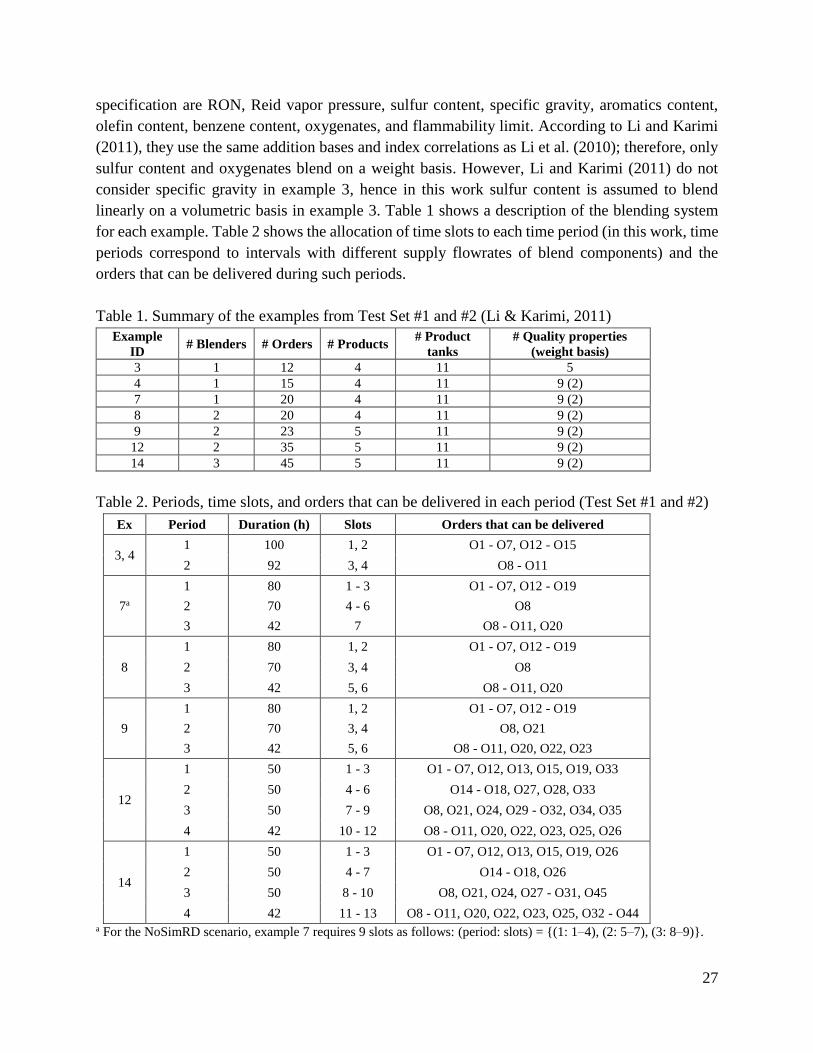
linearly on a volumetric basis in example 3. Table 1 shows a description of the blending system

for each example. Table 2 shows the allocation of time slots to each time period (in this work, time

periods correspond to intervals with different supply flowrates of blend components) and the

orders that can be delivered during such periods.

Table 1. Summary of the examples from Test Set #1 and #2 (Li & Karimi, 2011)

Example

ID # Blenders # Orders # Products

# Product

tanks

# Quality properties

(weight basis)

3 1 12 4 11 5

4 1 15 4 11 9 (2)

7 1 20 4 11 9 (2)

8 2 20 4 11 9 (2)

9 2 23 5 11 9 (2)

12 2 35 5 11 9 (2)

14 3 45 5 11 9 (2)

Table 2. Periods, time slots, and orders that can be delivered in each period (Test Set #1 and #2)

Ex Period Duration (h) Slots Orders that can be delivered

3, 4 1 100 1, 2 O1 - O7, O12 - O15

2 92 3, 4 O8 - O11

7a

1 80 1 - 3 O1 - O7, O12 - O19

2 70 4 - 6 O8

3 42 7 O8 - O11, O20

8

1 80 1, 2 O1 - O7, O12 - O19

2 70 3, 4 O8

3 42 5, 6 O8 - O11, O20

9

1 80 1, 2 O1 - O7, O12 - O19

2 70 3, 4 O8, O21

3 42 5, 6 O8 - O11, O20, O22, O23

12

1 50 1 - 3 O1 - O7, O12, O13, O15, O19, O33

2 50 4 - 6 O14 - O18, O27, O28, O33

3 50 7 - 9 O8, O21, O24, O29 - O32, O34, O35

4 42 10 - 12 O8 - O11, O20, O22, O23, O25, O26

14

1 50 1 - 3 O1 - O7, O12, O13, O15, O19, O26

2 50 4 - 7 O14 - O18, O26

3 50 8 - 10 O8, O21, O24, O27 - O31, O45

4 42 11 - 13 O8 - O11, O20, O22, O23, O25, O32 - O44 a For the NoSimRD scenario, example 7 requires 9 slots as follows: (period: slots) = {(1: 1–4), (2: 5–7), (3: 8–9)}.

28

Test set #2 consists of example number 4, 8, 12, and 14 from Li and Karimi (2011);

however, RON and MON properties are considered to blend nonlinearly following the ethyl RT-

70 models. RON index correlation from Li et al. (2010) was used to compute the actual RON

values and product specifications. Li and Karimi (2011) do not specify MON values, and these

were assumed in this work. For simplicity, MON minimum product specifications were set equal

to zero in order to observe only the effect of the RON constraint in the optimum. RON and MON

values and specifications are shown in Table 3.

Table 3. RON and MON values for examples from Test Set #2.

Property Blend Components

C1 C2 C3 C4 C5 C6 C7 C8 C9

RON 75 90.3 95.6 97.3 83 100 115 118 81

MON 66 80.8 80.5 91.7 74 100 109 100 72

Product specifications [min, max]

P1 P2 P3 P4 P5

RON [95, 200] [96, 200] [94, 200] [90, 200] [98, 200]

MON [0, 200] [0, 200] [0,200] [0, 200] [0, 200]

6. Computational Performance

The continuous-time blend scheduling models L-SimRD, L-NoSimRD, N-SimRD, and N-

NoSimRD were implemented in GAMS IDE 24.3.2. CPLEX 12.6 was used for MILP models, and

BARON 14.0.3 and ANTIGONE 1.1 were employed for MINLP models. CPLEX 12.6 and

ANTIGONE 1.1 were selected for LP and NLP models, respectively, required to compute the

lower bounds on the blend cost (Castillo & Mahalec, 2014a). All problems have been solved on

DELL PowerEdge T310 (Intel® Xeon® CPU, 2.40 GHz, and 12 GB RAM) running Windows

Server 2008 R2 OS.

6.1. Test set #1

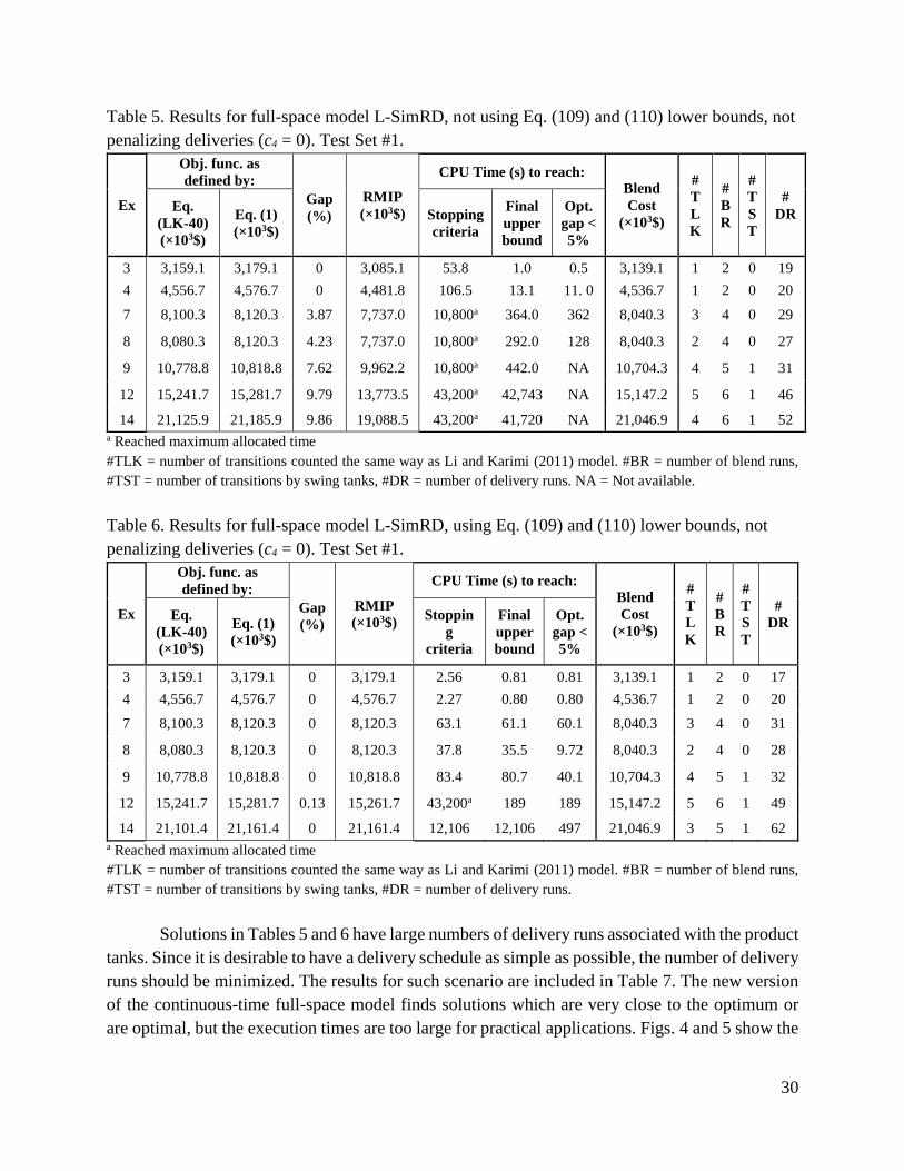
Table 4 shows the full-space model size for these examples, while Tables 5 and 6 show the

results for scenarios when multiple delivery runs from the tanks are not minimized (penalized).

Hence, these results are for the same kind of problems as those solved by Li and Karimi (2011).

In order to facilitate comparison with Li and Karimi (2011), the results in Table 5 and Table 6

show the objective function computed by Eq. (1) and its equivalent value in terms of Eq. (LK-40)

from Li and Karimi (2011). Note that Eq. (LK-40) does not take into account the transitions that

occur during the first time slot (i.e. slot n = 0).

For smaller examples, the computed results are the same as those by Li and Karimi (2011).

There is a discrepancy between the problem data as published and the solutions reported by Li and

29

Karimi (2011) for larger examples. Our recent communication with Dr. Li (Li, 2014) indicates that

the published problem description data for examples 9 and 14 have typographical errors. Hence,

the solutions presented here for examples 9 and 14 are for data as published and the comparison

with the published solution by Li and Karimi (2011) is not meaningful. The example 12 description

data as published are correct (Li, 2014). Since the solution of Example 12 as published by Li &

Karimi (2011) is lower than the lower bound for the blend cost (i.e. it is infeasible), it is not

meaningful to compare our solution of example 12 with the originally published solution.

In order to evaluate the impact of additional lower bounds, i.e. Eqs. (109) and (110), the

full-space continuous-time model, without penalizing multiple deliveries from tanks, has been

solved without these bounds (see Table 5) and with these bounds (see Table 6). Please note that

both tables contain the objective function as defined by Eq. (1) and the objective function as

defined by Li and Karimi (2011) in order to facilitate comparison with the previously published

results. Without additional lower bounds, the optimality gap cannot be closed for larger problems

even after 12 hours. With additional lower bounds, examples 3 to 9 are solved very rapidly,

example 14 is solved to optimality within approximately 3.5 hours, while example 12 is solved to

0.13% gap within 12 hours. The solution of the relaxed problem (i.e. RMIP) is reported as well.

Eq. (109) and (110) increase the RMIP solutions from 2 to almost 10%, depending on the example.

Table 4. Continuous-time full-space model size comparison for Test Set #1.

E

x

Li and Karimi (2011) NoSimRD Model L-NoSimRD-opt Model L-SimRD-opt

#

Slots # Eqs

#

Conts

#

Bins

#

Slots # Eqs

#

Conts

#

Bins

#

Slots # Eqs

#

Conts

#

Bins

3 3 2,987 799 246 4 3,910 1,251 306 4 5,134 1,432 306

4 3 3,479 925 285 4 4,512 1,404 342 4 6,060 1,639 342

7 7 10,337 2,381 986 9 10,515 3,298 753 7 10,660 2,940 571

8 6 11,491 2,244 949 6 8,881 2,446 553 6 11,737 2,769 553

9 6 12,635 2,391 1,015 6 9,780 2,569 594 6 12,876 2,915 594

12 12 34,151 6,572 3,050 12 22,203 6,205 1,317 12 30,051 7,008 1,317

14 13 49,097 8,508 3,989 13 31,135 8,012 1,628 13 43,165 8,945 1,628

#Slots = number of unit slots, #Eqs = equations, #Conts = continuous variables, and #Bins = binary variables.

30

Table 5. Results for full-space model L-SimRD, not using Eq. (109) and (110) lower bounds, not

penalizing deliveries (c4 = 0). Test Set #1.

Ex

Obj. func. as

defined by:

RMIP

(×103$)

CPU Time (s) to reach: Blend

Cost

(×103$)

#

T

L

K

#

B

R

#

T

S

T

#

DR Eq.

(LK-40)

(×103$)

Eq. (1)

(×103$)

Gap

(%) Stopping

criteria

Final

upper

bound

Opt.

gap <

5%

3 3,159.1 3,179.1 0 3,085.1 53.8 1.0 0.5 3,139.1 1 2 0 19

4 4,556.7 4,576.7 0 4,481.8 106.5 13.1 11. 0 4,536.7 1 2 0 20

7 8,100.3 8,120.3 3.87 7,737.0 10,800a 364.0 362 8,040.3 3 4 0 29

8 8,080.3 8,120.3 4.23 7,737.0 10,800a 292.0 128 8,040.3 2 4 0 27

9 10,778.8 10,818.8 7.62 9,962.2 10,800a 442.0 NA 10,704.3 4 5 1 31

12 15,241.7 15,281.7 9.79 13,773.5 43,200a 42,743 NA 15,147.2 5 6 1 46

14 21,125.9 21,185.9 9.86 19,088.5 43,200a 41,720 NA 21,046.9 4 6 1 52 a Reached maximum allocated time

#TLK = number of transitions counted the same way as Li and Karimi (2011) model. #BR = number of blend runs,

#TST = number of transitions by swing tanks, #DR = number of delivery runs. NA = Not available.

Table 6. Results for full-space model L-SimRD, using Eq. (109) and (110) lower bounds, not

penalizing deliveries (c4 = 0). Test Set #1.

Ex

Obj. func. as

defined by:

RMIP

(×103$)

CPU Time (s) to reach:

Blend

Cost

(×103$)

#

T

L

K

#

B

R

#

T

S

T

#

DR Eq.

(LK-40)

(×103$)

Eq. (1)

(×103$)

Gap

(%) Stoppin

g

criteria

Final

upper

bound

Opt.

gap <

5%

3 3,159.1 3,179.1 0 3,179.1 2.56 0.81 0.81 3,139.1 1 2 0 17

4 4,556.7 4,576.7 0 4,576.7 2.27 0.80 0.80 4,536.7 1 2 0 20

7 8,100.3 8,120.3 0 8,120.3 63.1 61.1 60.1 8,040.3 3 4 0 31

8 8,080.3 8,120.3 0 8,120.3 37.8 35.5 9.72 8,040.3 2 4 0 28

9 10,778.8 10,818.8 0 10,818.8 83.4 80.7 40.1 10,704.3 4 5 1 32

12 15,241.7 15,281.7 0.13 15,261.7 43,200a 189 189 15,147.2 5 6 1 49

14 21,101.4 21,161.4 0 21,161.4 12,106 12,106 497 21,046.9 3 5 1 62 a Reached maximum allocated time

#TLK = number of transitions counted the same way as Li and Karimi (2011) model. #BR = number of blend runs,

#TST = number of transitions by swing tanks, #DR = number of delivery runs.

Solutions in Tables 5 and 6 have large numbers of delivery runs associated with the product

tanks. Since it is desirable to have a delivery schedule as simple as possible, the number of delivery

runs should be minimized. The results for such scenario are included in Table 7. The new version

of the continuous-time full-space model finds solutions which are very close to the optimum or

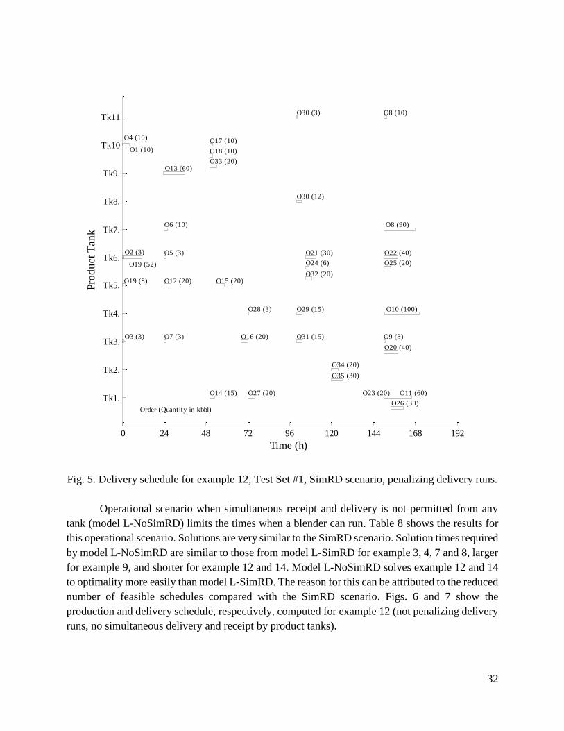
are optimal, but the execution times are too large for practical applications. Figs. 4 and 5 show the

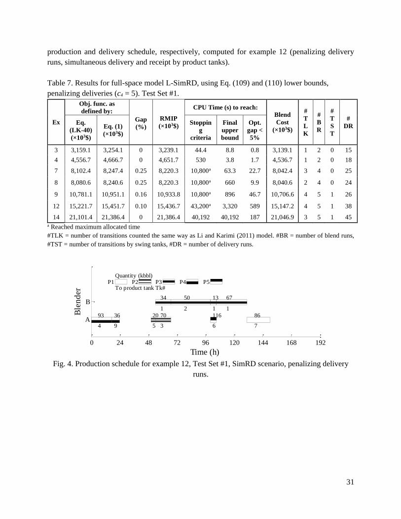
31

production and delivery schedule, respectively, computed for example 12 (penalizing delivery

runs, simultaneous delivery and receipt by product tanks).

Table 7. Results for full-space model L-SimRD, using Eq. (109) and (110) lower bounds,

penalizing deliveries (c4 = 5). Test Set #1.

Ex

Obj. func. as

defined by:

RMIP

(×103$)

CPU Time (s) to reach:

Blend

Cost

(×103$)

#

T

L

K

#

B

R

#

T

S

T

#

DR Eq.

(LK-40)

(×103$)

Eq. (1)

(×103$)

Gap

(%) Stoppin

g

criteria

Final

upper

bound

Opt.

gap <

5%

3 3,159.1 3,254.1 0 3,239.1 44.4 8.8 0.8 3,139.1 1 2 0 15

4 4,556.7 4,666.7 0 4,651.7 530 3.8 1.7 4,536.7 1 2 0 18

7 8,102.4 8,247.4 0.25 8,220.3 10,800a 63.3 22.7 8,042.4 3 4 0 25

8 8,080.6 8,240.6 0.25 8,220.3 10,800a 660 9.9 8,040.6 2 4 0 24

9 10,781.1 10,951.1 0.16 10,933.8 10,800a 896 46.7 10,706.6 4 5 1 26

12 15,221.7 15,451.7 0.10 15,436.7 43,200a 3,320 589 15,147.2 4 5 1 38

14 21,101.4 21,386.4 0 21,386.4 40,192 40,192 187 21,046.9 3 5 1 45 a Reached maximum allocated time

#TLK = number of transitions counted the same way as Li and Karimi (2011) model. #BR = number of blend runs,

#TST = number of transitions by swing tanks, #DR = number of delivery runs.

Fig. 4. Production schedule for example 12, Test Set #1, SimRD scenario, penalizing delivery

runs.

0 24 48 72 96 120 144 168 192

A

B

Time (h)

Ble

nd

er

93

4

36

9

20

5

70

3

116

6

86

7

34

1

50

2

13

1

67

1

P1 P2 P3 P4 P5Quantity (kbbl)

To product tank Tk#

32

Fig. 5. Delivery schedule for example 12, Test Set #1, SimRD scenario, penalizing delivery runs.

Operational scenario when simultaneous receipt and delivery is not permitted from any

tank (model L-NoSimRD) limits the times when a blender can run. Table 8 shows the results for

this operational scenario. Solutions are very similar to the SimRD scenario. Solution times required

by model L-NoSimRD are similar to those from model L-SimRD for example 3, 4, 7 and 8, larger

for example 9, and shorter for example 12 and 14. Model L-NoSimRD solves example 12 and 14

to optimality more easily than model L-SimRD. The reason for this can be attributed to the reduced

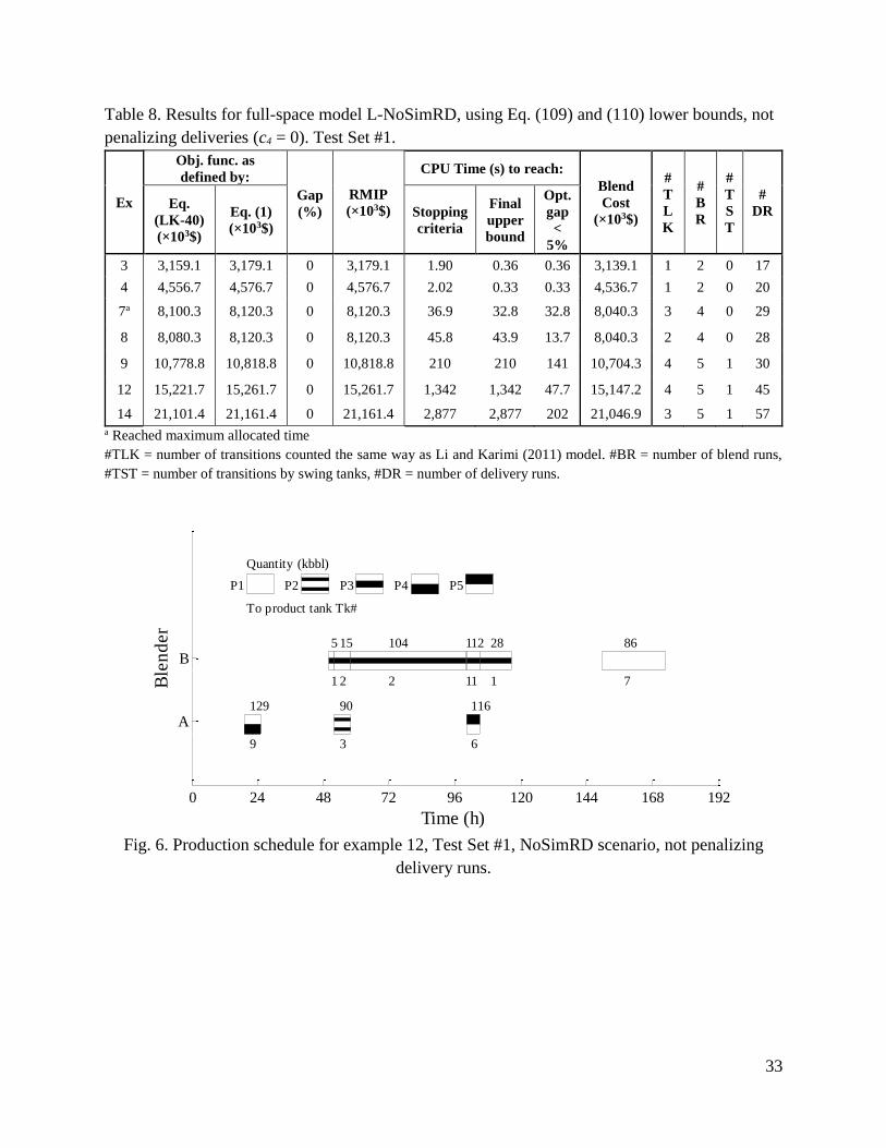
number of feasible schedules compared with the SimRD scenario. Figs. 6 and 7 show the

production and delivery schedule, respectively, computed for example 12 (not penalizing delivery

runs, no simultaneous delivery and receipt by product tanks).

0 24 48 72 96 120 144 168 192

Tk1.

Tk2.

Tk3.

Tk4.

Tk5.

Tk6.

Tk7.

Tk8.

Tk9.

Tk10

Tk11

Time (h)

Pro

du

ct

Tan

k

O11 (60)O14 (15) O23 (20)

O26 (30)

O27 (20)

O34 (20)

O35 (30)

O3 (3) O7 (3) O9 (3)O16 (20)

O20 (40)

O31 (15)

O10 (100)O28 (3) O29 (15)

O12 (20) O15 (20)O19 (8)

O2 (3) O5 (3)

O19 (52)

O21 (30) O22 (40)

O24 (6) O25 (20)

O32 (20)

O6 (10) O8 (90)

O30 (12)

O13 (60)

O1 (10)

O4 (10)O17 (10)

O18 (10)

O33 (20)

O8 (10)O30 (3)

Order (Quantity in kbbl)

33

Table 8. Results for full-space model L-NoSimRD, using Eq. (109) and (110) lower bounds, not

penalizing deliveries (c4 = 0). Test Set #1.

Ex

Obj. func. as

defined by:

RMIP

(×103$)

CPU Time (s) to reach:

Blend

Cost

(×103$)

#

T

L

K

#

B

R

#

T

S

T

#

DR Eq.

(LK-40)

(×103$)

Eq. (1)

(×103$)

Gap

(%) Stopping

criteria

Final

upper

bound

Opt.

gap

<

5%

3 3,159.1 3,179.1 0 3,179.1 1.90 0.36 0.36 3,139.1 1 2 0 17

4 4,556.7 4,576.7 0 4,576.7 2.02 0.33 0.33 4,536.7 1 2 0 20

7a 8,100.3 8,120.3 0 8,120.3 36.9 32.8 32.8 8,040.3 3 4 0 29

8 8,080.3 8,120.3 0 8,120.3 45.8 43.9 13.7 8,040.3 2 4 0 28

9 10,778.8 10,818.8 0 10,818.8 210 210 141 10,704.3 4 5 1 30

12 15,221.7 15,261.7 0 15,261.7 1,342 1,342 47.7 15,147.2 4 5 1 45

14 21,101.4 21,161.4 0 21,161.4 2,877 2,877 202 21,046.9 3 5 1 57 a Reached maximum allocated time

#TLK = number of transitions counted the same way as Li and Karimi (2011) model. #BR = number of blend runs,

#TST = number of transitions by swing tanks, #DR = number of delivery runs.

Fig. 6. Production schedule for example 12, Test Set #1, NoSimRD scenario, not penalizing

delivery runs.

0 24 48 72 96 120 144 168 192

A

B

Time (h)

Ble

nd

er

129

9

90

3

116

6

5

1

15

2

104

2

1

1

12

1

28

1

86

7

P1 P2 P3 P4 P5

Quantity (kbbl)

To product tank Tk#

34

Fig. 7. Delivery schedule for example 12, Test Set #1, NoSimRD scenario, not penalizing

delivery runs.

6.2. Test set #2

Nonlinear problems have been solved for the scenario when no simultaneous receipt and

delivery by product tanks is allowed, and when delivery runs are not penalized. Eqs. (109) and

(110) were included in the model. The size of model N-NoSimRD-opt for Test Set #2 examples is

shown in Table 9. As expected, the number of binary variables remains the same, and the number

of equations and continuous variables increased slightly due to the addition of Eqs. (111-a)–(111-

l), (112) and (113). The number of nonlinear terms is presented as well. Table 10 shows the results

obtained by global MINLP solvers BARON and ANTIGONE. Only small-scale example 4 is

solved to optimality. Example 8 is solved very close to optimality within the allocated time of 3

0 24 48 72 96 120 144 168 192

Tk1.

Tk2.

Tk3.

Tk4.

Tk5.

Tk6.

Tk7.

Tk8.

Tk9.

Tk10

Tk11

Time (h)

Pro

du

ct

Tan

k

O14 (15) O23 (20)

O26 (21)

O27 (20)

O11 (60)

O26 (9)

O34 (20)

O35 (30)

O3 (3) O5 (3) O9 (3)

O15 (8)

O15 (12)

O16 (20) O20 (40)

O31 (15)

O10 (25)

O2 (2) O7 (3)

O12 (20)O19 (3)

O2 (1)

O19 (57)

O21 (30) O22 (40)

O24 (6)

O25 (20)

O32 (20)

O6 (0) O8 (86)O33 (14)

O6 (10) O8 (2)

O10 (75)O13 (60) O28 (3) O29 (15)

O1 (10)

O4 (10)

O8 (9)O18 (10) O30 (15)O33 (6)

O8 (2)O17 (10)

Order (Quantity in kbbl)

35

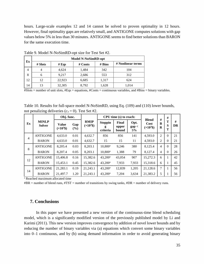
hours. Large-scale examples 12 and 14 cannot be solved to proven optimality in 12 hours.

However, final optimality gaps are relatively small, and ANTIGONE computes solutions with gap

values below 5% in less than 30 minutes. ANTIGONE seems to find better solutions than BARON

for the same execution time.

Table 9. Model N-NoSimRD-opt size for Test Set #2.

Ex Model N-NoSimRD-opt

# Slots # Eqs # Conts # Bins # Nonlinear terms

4 4 4,624 1,484 342 104

8 6 9,217 2,686 553 312

12 12 22,923 6,685 1,317 624

14 13 32,305 8,792 1,628 1,014

#Slots = number of unit slots, #Eqs = equations, #Conts = continuous variables, and #Bins = binary variables.

Table 10. Results for full-space model N-NoSimRD, using Eq. (109) and (110) lower bounds,

not penalizing deliveries (c4 = 0). Test Set #2.

Ex MINLP

Solver

Obj. func.

RMIP

(×103$)

CPU time (s) to reach: Blend

Cost

(×103$)

#

B

R

#

T

S

T

#

DR Value

(×103$)

Gap

(%)

Stoppin

g

criteria

Final

upper

bound

Opt.

gap <

5%

4 ANTIGONE 4,633.0 0.01 4,632.7 856 856 141 4,593.0 2 0 21

BARON 4,633.0 0.01 4,632.7 15 15 11 4,593.0 2 0 21

8 ANTIGONE 8,205.4 0.03 8,203.1 10,800a 9,246 380 8,125.4 4 0 28

BARON 8,207.4 0.05 8,203.1 10,800a 1,388 79 8,127.4 4 0 26

12 ANTIGONE 15,406.8 0.16 15,382.6 43,200a 43,054 907 15,272.3 6 1 42

BARON 15,453.1 0.45 15,382.6 43,200a 7,933 7,933 15,318.6 6 1 45

14 ANTIGONE 21,283.1 0.19 21,243.1 43,200a 12,839 1,205 21,128.6 7 1 56

BARON 21,497.7 1.20 21,243.1 43,200a 7,204 3,634 21,383.2 5 1 56 a Reached maximum allocated time

#BR = number of blend runs, #TST = number of transitions by swing tanks, #DR = number of delivery runs.

7. Conclusions

In this paper we have presented a new version of the continuous-time blend scheduling

model, which is a significantly modified version of the previously published model by Li and

Karimi (2011). This new version improves convergence by addition of novel lower bounds and by

reducing the number of binary variables via (a) equations which convert some binary variables

into 0–1 continuous, and by (b) using demand information in order to avoid generating binary

36

variables where orders cannot be delivered. The model also includes additional operational

features such as penalty for deliveries of the same order from different product tanks, product and

blender-dependent minimum setup times, maximum delivery rate from component tanks, and a

threshold volume for each blend.

These modifications significantly improve convergence of the model, to the extent that

previously published unsolved large linear blend scheduling examples have been solved to

optimality or very close to it. The execution times are two to three orders of magnitude shorter

than originally published times. Satisfactory convergence for medium size nonlinear blend

scheduling problems (ethyl RT-70 equations for octane blending) has been obtained applying

global MINLP solvers and the results are very close to optimality. Solutions with optimality gap

smaller than 5% were found in less than 30 min for the two large-scale problems considered in this

work. This has motivated our work on a new type of scheduling algorithm which is described in

the companion paper (Castillo-Castillo and Mahalec, 2015).

Acknowledgments

Support by Ontario Research Foundation and McMaster Advanced Control Consortium is

gratefully acknowledged.

Appendix A. Supplementary data

Supplementary data associated with this article can be found, in the online version, at

http://dx.doi.org/10.1016/j.compchemeng.2015.08.003.

37

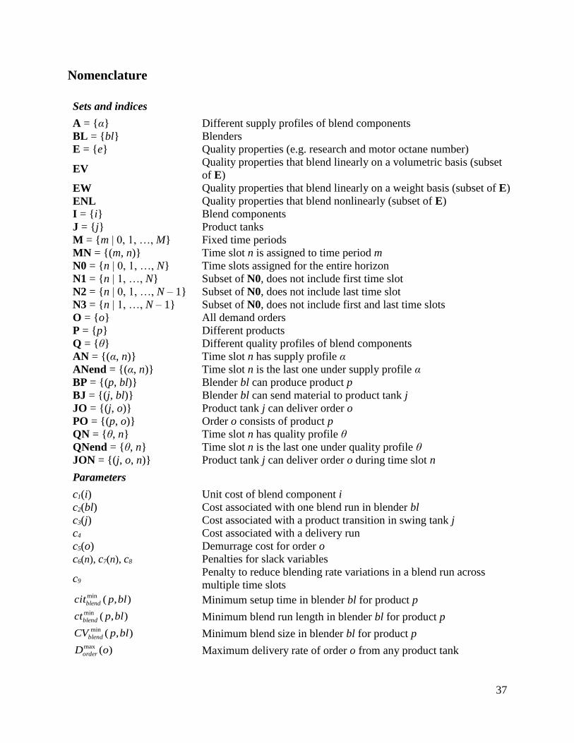
Nomenclature

Sets and indices

A = {α} Different supply profiles of blend components

BL = {bl} Blenders

E = {e} Quality properties (e.g. research and motor octane number)

EV Quality properties that blend linearly on a volumetric basis (subset

of E)

EW Quality properties that blend linearly on a weight basis (subset of E)

ENL Quality properties that blend nonlinearly (subset of E)

I = {i} Blend components

J = {j} Product tanks

M = {m | 0, 1, …, M} Fixed time periods

MN = {(m, n)} Time slot n is assigned to time period m

N0 = {n | 0, 1, …, N} Time slots assigned for the entire horizon

N1 = {n | 1, …, N} Subset of N0, does not include first time slot

N2 = {n | 0, 1, …, N – 1} Subset of N0, does not include last time slot

N3 = {n | 1, …, N – 1} Subset of N0, does not include first and last time slots

O = {o} All demand orders

P = {p} Different products

Q = {θ} Different quality profiles of blend components

AN = {(α, n)} Time slot n has supply profile α

ANend = {(α, n)} Time slot n is the last one under supply profile α

BP = {(p, bl)} Blender bl can produce product p

BJ = {(j, bl)} Blender bl can send material to product tank j

JO = {(j, o)} Product tank j can deliver order o

PO = {(p, o)} Order o consists of product p

QN = {θ, n} Time slot n has quality profile θ

QNend = {θ, n} Time slot n is the last one under quality profile θ

JON = {(j, o, n)} Product tank j can deliver order o during time slot n

Parameters

c1(i) Unit cost of blend component i

c2(bl) Cost associated with one blend run in blender bl

c3(j) Cost associated with a product transition in swing tank j

c4 Cost associated with a delivery run

c5(o) Demurrage cost for order o

c6(n), c7(n), c8 Penalties for slack variables

c9 Penalty to reduce blending rate variations in a blend run across

multiple time slots

),(min blpcitblend Minimum setup time in blender bl for product p

),(min blpctblend Minimum blend run length in blender bl for product p

),(min blpCVblend Minimum blend size in blender bl for product p

)(max oDorder Maximum delivery rate of order o from any product tank

38

)(max jDpr Maximum delivery rate of product tank j

Demand(o) Demand quantity of order o

),( iFbc Flow rate of blend component i for supply profile α

)(min blFblend, )(max blFblend

Minimum and maximum blending rates of blender bl

),(max bliFcomp Maximum pumping rate of blend component tank i to blender bl

)(end

bcFT Time when supply profile α ends

H Length of the entire scheduling horizon

),,( eiQbc Quality e of blend component i during quality profile θ

),(min epQpr , ),(max epQpr Minimum and maximum specifications for quality property e and

product p

)(end

bcQT Time when quality profile θ ends

),(min pir , ),(max pir Minimum and maximum composition of component i in product p

expsw Minimum number of blend runs expected in the blenders along the

scheduling horizon

)(mT start , )(mT end Start and end time of period m

)(oTO start

order, )(oTO end

order Start and end time of delivery window for order o

expue Minimum number of product changeovers expected in the swing

tanks along the scheduling horizon

)(min iVbc, )(max iVbc

Minimum and maximum inventory limits of blend component i

)(min jVpr , )(max jVpr Minimum and maximum inventory limits of product tank j

)(i Density of blend component i

Binary variables

),,( npju If equal to 1, product tank j is storing product p during slot n

),,( nbljv If equal to 1, blender bl is sending material to product tank j during

slot n

),,( nojz If equal to 1, product tank j delivers material to order o during slot n

0-1 Continuous variables

),( nblsw If equal to 1, a blend run is starting in blender bl at the end of slot n

),( nblw If equal to 1, blender bl is idle during slot n

),,( nblpx If equal to 1, blender bl is processing product p during slot n

),( nblxe If equal to 1, blender bl is changing its state at the end of slot n

),,( nbliy If equal to 1, component i is being fed to blender bl during slot n

),,( nojze If equal to 1, product tank j change its state at the end of slot n (i.e. it

starts or stops to deliver material)

Continuous variables

),( nblctblend Underestimator of the cumulative running time of blender bl at the

end of slot n

),( nblcitblend Underestimator of the cumulative idle time of blender bl at the

beginning of slot n

39

),( nblCVblend

Underestimator of the cumulative volume blended up to slot n by

blender bl

),,( nojDVpr Volume delivered from product tank j to order o during slot n

),( nblitblend Idle time of blender bl at time slot n

),,( neblQpr Quality e of the product from blender bl during slot n

),(),,( niSniS bcbc

Positive and negative slack variables for the blend component

inventories

)(),( oSoS orderorder

Positive and negative slack variables for each order fulfillment

),(),,( njSnjS prpr

Positive and negative slack variables for the product inventories

),( nblTb End time of a blender slot n

),( niTbc End time of a component tank slot n

),( njTpr End time of a product tank slot n

),( nbltblend Running time of blender bl at time slot n

),,( nojtdorder

Time dedicated to deliver material from product tank j to order o

during slot n

)(otdem Time required to complete order o after the end of the corresponding

delivery window

),,( nojtsorder Time when product tank j starts to deliver material to order o during

slot n

),( nittbc Time when component tank i stops sending material to any blender

during slot n

),( njue If equal to 1, product tank j changes its service at the end of slot n

),( niVbc Inventory level of component tank i at the end of slot n

),( nblVblend Volume blended during slot n by blender bl

)(, iV aggcomp Volume required of component i according to the aggregated model

solution

),,( nbliVcomp Volume of component i used in blender bl during slot n

),( njVpr Inventory level of product tank j at the end of slot n

),,( nbljVtrans Volume transferred from blender bl to product tank j during slot n

References

Castillo PA, Kelly JD, Mahalec V. Inventory pinch algorithm for gasoline blend planning. AIChE

J 2013; 59(10):3748-3766.

Castillo PA, Mahalec V. Inventory pinch based, multiscale models for integrated planning and

scheduling‐part I: Gasoline blend planning. AIChE J 2014a; 60(6):2158-2178.

Castillo PA, Mahalec V. Inventory pinch based, multiscale models for integrated planning and

scheduling-part II: Gasoline blend scheduling. AIChE J 2014b; 60(7):2475-2497.

40

Castillo PA, Mahalec V. Inventory pinch gasoline blend scheduling algorithm combining discrete-

and continuous-time models. Comput Chem Eng 2015; “submitted”.

Floudas CA, Lin X. Continuous-time vs discrete-time approaches for scheduling of chemical

processes: a review. Comput Chem Eng 2004; 28:2109-2129.

Harjunkoski I, Maravelias CT, Bongers P, Castro PM, Engell S, Grossmann IE, Hooker J, Mendez

C, Sand G, Wassick J. Scope for industrial applications of production scheduling models and

solution methods. Comput Chem Eng 2014; 62:161-193.

Healey WC, Maasen CW, Peterson RT. A new approach to blending octanes. In: Proc. 24th

Meeting of American Petroleum Institute’s Division of Refining. New York, 1959.

Jia Z, Ierapetritou M. Mixed-integer linear programming model for gasoline blending and

distribution scheduling. Ind Eng Chem Res 2003; 42:825-835.

Joly M, Pinto JM. Mixed-integer programming techniques for the scheduling problem of fuel oil

and asphalt production. Inst Chem Eng 2003; 81:427-447.

Kolodziej SP, Grossmann IE, Furman KC, Sawayac NW. A discretization-based approach for the

optimization of the multiperiod blend scheduling problem. Comput Chem Eng 2013; 53:122-

142.

Li J. Personal communication. 2014.

Li J, Karimi IA. Scheduling gasoline blending operations from recipe determination to shipping

using unit slots. Ind Eng Chem Res 2011; 50:9156–9174.

Li J, Karimi IA, Srinivasan R. Recipe determination and scheduling of gasoline blending

operations. AIChE J 2010; 56:441-465.

Maravelias CT. General framework and modeling approach classification for chemical production

scheduling. AIChE J 2012; 58:1812-1828.

Mendez CA, Grossmann IE, Harjunkoski I, Kabore P. A simultaneous optimization approach for

off-line blending. Comput Chem Eng 2006; 30:614–634.

Neiro SMS, Murata VV, Pinto JM. Hybrid time formulation for diesel blending and distribution

scheduling. Ind Eng Chem Res 2014; 53:17124-17134.

Singh A, Forbes JF, Vermeer PJ, Woo SS. Model-based real-time optimization of automotive

gasoline blending operations. J Process Control 2000; 10:43-58.

Sundaramoorthy A, Maravelias CT. Computational study of network-based mixed-integer

programming approaches for chemical production scheduling. Ind Eng Chem Res 2011;

50:5023-5040.

Velez S, Maravelias CT. Theoretical framework for formulating MIP scheduling models with

multiple and non-uniform discrete-time grids. Comput Chem Eng 2015; 72:233-254.