Embed Size (px)
Citation preview

Article from:
North American Actuarial Journal
Vol.13 No.1
1
A QUANTITATIVE COMPARISON OF STOCHASTICMORTALITY MODELS USING DATA FROM
ENGLAND AND WALES AND THE UNITED STATESAndrew J. G. Cairns,* David Blake,† Kevin Dowd,‡ Guy D. Coughlan,§ David Epstein,§
Alen Ong,§ and Igor Balevich�
ABSTRACT
We compare quantitatively eight stochastic models explaining improvements in mortality rates inEngland and Wales and in the United States. On the basis of the Bayes Information Criterion (BIC),we find that, for higher ages, an extension of the Cairns-Blake-Dowd (CBD) model that incor-porates a cohort effect fits the England and Wales males data best, while for U.S. males data, theRenshaw and Haberman (RH) extension to the Lee and Carter model that also allows for a cohorteffect provides the best fit. However, we identify problems with the robustness of parameterestimates under the RH model, calling into question its suitability for forecasting. A different ex-tension to the CBD model that allows not only for a cohort effect, but also for a quadratic ageeffect, while ranking below the other models in terms of the BIC, exhibits parameter stabilityacross different time periods for both datasets. This model also shows, for both datasets, thatthere have been approximately linear improvements over time in mortality rates at all ages, butthat the improvements have been greater at lower ages than at higher ages, and that there aresignificant cohort effects.
1. INTRODUCTION
It has become increasingly clear that mortality improvements in countries where reliable data exist aredriven by an underlying process that is stochastic. Since the early 1990s a number of stochastic modelshave been developed to analyze these mortality improvements. These include the Lee-Carter model andits extensions (Lee and Carter 1992; Brouhns, Denuit, and Vermunt 2002; Renshaw and Haberman2003, 2006; Continuous Mortality Investigation Bureau [CMI] 2005, 2006); the P-splines model (Cur-rie, Durban, and Eilers 2004; Currie 2006; CMI 2005, 2006), and the Cairns-Blake-Dowd (CBD 2006b)model (a stochastic version of the Perks 1932 model). A number of recent papers have sought tocompare different mortality models, including Wong-Fupuy and Haberman (2004), Renshaw and Ha-berman (RH, 2006), and CMI (2005, 2006, 2007). Renshaw and Haberman (2006), for example, com-pare models in a quantitative fashion by analyzing the pattern of standardized residuals against age,year of observation, and year of birth. However, so far as we are aware, no studies have used formal
* Maxwell Institute for Mathematical Sciences and Department of Actuarial Mathematics and Statistics, Heriot-Watt University, Edinburgh, EH144AS, United Kingdom, [email protected].† Pensions Institute, Cass Business School, City University, 106 Bunhill Row, London, EC1Y 8TZ, United Kingdom.‡ Centre for Risk and Insurance Studies, Nottingham University Business School, Jubilee Campus, Nottingham, NG8 1BB, United Kingdom.§ Pension ALM Group, JPMorgan Chase Bank, 125 London Wall, London, EC2Y 5AJ, United Kingdom.� Pension Advisory Group, JPMorgan Securities Inc., 270 Park Avenue, New York, NY 10017-2070.

2 NORTH AMERICAN ACTUARIAL JOURNAL, VOLUME 13, NUMBER 1
model selection criteria to compare and rank a variety of nested and non-nested models. This studyundertakes such a comparison.
We consider a range of both existing and new models.1 In the early part of the paper, we comparethese on the basis of a set of desirable, qualitative properties: parsimony, transparency, ability to gen-erate sample paths, incorporation of cohort effects (see Willets 1999, 2004; Richards, Kirkby, andCurrie 2006), and ability to produce a nontrivial correlation structure. The study then pays considerableattention to two important quantitative criteria that can be evaluated only when each model is fittedto the data: consistency with historical data, and robustness of parameter estimates relative to therange of data employed.2
Our analysis focuses on mortality at higher ages (60–89), given our interest in pension-related ap-plications where the risk associated with longer-term cash flows is primarily linked to uncertainty infuture rates of mortality at higher ages. For models M5–M8, the focus on this higher age range allowsus to exploit the relatively simple log-linear structure of the mortality curve resulting in a family ofmultifactor models that have parsimonious age effects.
We find that no single model dominates on the basis of all the above criteria. If we rank modelsusing an objective model selection criterion based on the statistical quality of fit, then an extension ofthe CBD (2006b) model fits the England and Wales data best, while the RH (2006) model fits the U.S.data best. However, if we take the robustness of parameter estimates into account, then the preferredmodel is a different extension of the CBD model that allows for both a cohort effect and a period effectthat is quadratic in age.
1.1 NotationWe consider eight models in this paper, and it is important that we use consistent and clear notationthroughout:
• Calendar year t is defined as running from time t to time t � 1.• We define mc(t, x) to be the crude (i.e., unsmoothed) death rate for age x in calendar year t. More
specifically,
Number of deaths during calendar year t aged x last birthdaym (t, x) � .c Average population during calendar year t aged x last birthday
The average population is usually approximated by an estimate of the population aged x last birthdayin the middle of the calendar year. The underlying death rate is then m(t, x), which is equal to theexpected deaths divided by the exposure.
• A second measure of mortality is the mortality rate q(t, x). This is the probability that an individualaged exactly x at exact time t will die between t and t � 1.
• A third measure is the force of mortality, �(t, x). This is interpreted as the instantaneous death rateat exact time t for individuals aged exactly x at time t. For these individuals, for small dt, the prob-ability of death between t and t � dt is approximately �(t, x) � dt.
• For individuals who die aged x last birthday, in year t we use the convention that t � x is the yearof birth. However, the precise date of birth might be any time between January 1 in calendar yeart � x � 1 and December 31 in calendar year t � x. For notational compactness we will sometimesuse c � t � x.
1 All models are described in the paper at the outset. However, the new models (labeled M6–M8) were developed in response to perceivedproblems with the original five models (M1–M5) as well as building on the strengths of these models.2 An earlier version of this paper, with the same title, looked in more detail at the underlying data and empirical illustrations of the cohorteffect. See http://www.ma.hw.ac.uk/�andrewc/papers/.

A QUANTITATIVE COMPARISON OF STOCHASTIC MORTALITY MODELS 3
1.2 Relationship between m(t, x) and q(t, x)The death rate, m(t, x), and the mortality rate, q(t, x), are typically very close to one another in value.With a simple assumption, we can formalize this relationship more precisely:
Assumption 1: For integers t and x, and for all 0 � s, u � 1, �(t � s, x � u) � �(t, x): that is, the force ofmortality remains constant over each year of integer age and over each calendar year.
This implies the following:
a. m(t, x) � �(t, x)b. q(t, x) � 1 � exp[��(t, x)] � 1 � exp[�m(t, x)].
Relationship (a) is often used in the analysis of death rate data (see, e.g., Brouhns, Denuit, and Vermunt2002). Relationship (b) is useful in the analysis of parametric models for mortality that are formulatedin terms of q(t, x).
Assumption 1 does not normally hold exactly, but the resulting relationship between m(t, x) andq(t, x) is generally felt to provide an accurate approximation.
2. DATA
We now discuss the general characteristics of both the England and Wales and the U.S. male data. Theprimary motivation for this study is to compare various mortality models and determine which are bestsuited to forecasting mortality at higher ages. This reflects a concern with longevity risk—the risk thatrealized survival rates might be higher than anticipated—to which pension plans and annuity providersare exposed. As a consequence, we use data at higher ages only (ages 60–89 inclusive) when we makeour comparisons of the different models.
2.1 England and Wales: Crude Death RatesIn this paper we use crude mortality rates for England and Wales (EW) males between 1961 and 2004.3
As ‘‘stylized facts’’ we can observe that over this period mortality rates have been declining at all ages,they have been declining at different rates at different ages, and they have been declining erratically(see, e.g., Cairns, Blake, and Dowd 2006a, Fig. 1.2).
A typical dataset consists of numbers of deaths, D(t, x), and the corresponding exposures, E(t, x),over a range of years t and ages x. Numbers of deaths are normally regarded as being reasonablyaccurate, although the recorded age at death is believed to be less accurate at very high ages. Theexposure E(t, x) represents the average, during calendar year t, of the number of people alive who wereaged x last birthday. This quantity is normally not known with a high degree of accuracy, even in censusyears, and has to be estimated by the Office for National Statistics (ONS) (or its equivalent in othercountries), taking account of recorded births and deaths and net immigration.
In the analysis that follows we shall exclude a number of seemingly unreliable data points (t, x):
• The 1886 cohort (i.e., t � x � 1886). Death rates for this cohort became markedly out of line withneighboring cohorts during the 1960s. This might be the result of poorly calculated exposures (i.e.,estimates of average population size at each age).
3 Data for this period were provided by the United Kingdom’s Office for National Statistics. The Human Mortality Database (www.mortality.org)and LifeMetrics (www.lifemetrics.com) also provide useful sources of data. Both web sites include thorough technical documentation to supportthe data. In their analyses of the Lee and Carter (1992), Renshaw and Haberman (2006), and P-splines (Currie, Durban, and Eilers 2004)models, CMI (2005, 2006, 2007) look at females as well as males data, and life-office assured lives’ data as well as national population data.

4 NORTH AMERICAN ACTUARIAL JOURNAL, VOLUME 13, NUMBER 1
• Death rates at and above age 85 in the years up to and including 1970. Accurate exposures were notestimated by the ONS (or its predecessors) at these ages until 1971.
Additionally, because some of the models we are fitting are cohort models, we will exclude all cohortsthat have fewer than five observations (after taking account of the exclusions above).4 The rationalefor including a ‘‘cohort effect’’ lies in an analysis of the rates at which mortality has been improvingat different ages and in different years (see Willets 2004; Richards, Kirkby, and Kelly 2006). Cohortsborn around 1930 experienced strong rates of improvement between ages 40 and 70 relative to, say,cohorts born 10 years earlier or 10 years later. For its part, the cohort born around 1950 seems tohave experienced worse mortality than the immediately preceeding cohorts.
2.2 United States: Crude Death RatesThis paper also analyzes data for U.S. males aged 60 to 89 over the period 1968–2003.5 We will focuson those aspects of the U.S. data that are different from the EW data.
With the EW data in a given year, t, we have identified (CBD 2006b) that logit q(t, x) (i.e.,log[q(t, x)/(1 � q(t, x))]) is reasonably linear in x. Although this is approximately true for the U.S.data, we found that, in some years, there is a small degree of curvature in the plot of logit q(t, x)against x. The curvature is not all that prominent, but it does turn out to be significant when wecompare models with and without a quadratic term in logit q(t, x), and it is an effect that changesover time. Although a cohort effect is evident in the U.S. data, the magnitude of the effect above age60 is much smaller than the EW cohort effect.
Accurate exposures data are not available for the period 1968–1979 for ages above 84. Consequentlywe have used data for ages 85–89 only after 1979. Issues relating to the accuracy of mortality data athigher ages are explored further by Anderson (1999).
In contrast with the EW data, the U.S. data do not appear to have any individual cohorts that haveidentifiable problems. However, we found that the exposures data were, in general, less reliable asestimates of the underlying population sizes at specific ages in specific years.6 This is most apparentif we follow the exposures data for a specific cohort over time.7 Exposures data for cohorts born in1928, 1918, 1908, and 1898 are plotted in Figure 1. We would normally expect to see a relativelysmooth progression in the exposures data from one year to the next. The decrease in the exposurefrom one year to the next should reflect the numbers of deaths and net immigration from the cohort.If net immigration is zero, this should result in a fairly smooth, downwards progression of values ineach plot. Instead, we see for each of the cohorts in Figure 1 that the pattern is somewhat erratic,especially for the top left plot. This might be explained by a volatile pattern of net immigration. How-ever, it could also be explained by errors in the underlying data (particularly the exposures data). Thecorresponding plots for EW are much smoother.
4 The reliability of the estimates of the cohort parameters (defined later) depends on the number of observations for each cohort. At one(i)�t�x
extreme, if we have just one observation, then the parameter can be chosen so that the fitted death rate is exactly equal to the observed(i)�t�x
rate, a ‘‘quality of fit’’ that can be achieved without affecting any of the other estimated death rates. In effect, the single observation allowsus to overfit the model, whereas the estimated parameter is, in reality, subject to substantial parameter uncertainty. With more observations(i)�t�x
in a given cohort, the estimated parameter becomes more reliable. Consequently we wish to exclude cohorts that have too few obser-(i)�t�x
vations. However, if we exclude too many cohorts, then we are left with relatively little data. We therefore adopt a compromise and excludecohorts with fewer than five observations.5 Data are available for higher ages, but, as previously discussed in the case of EW, age at death is often misreported at these high ages,resulting in unreliable estimated death rates at these ages.6 For further explanation, see Section 3.7 For example, if we follow exposures data for the ‘‘1920’’ cohort, then we look at the sequence E(1920, 0), E(1921, 1), . . . , E(1980, 60),E(1981, 61), . . . .
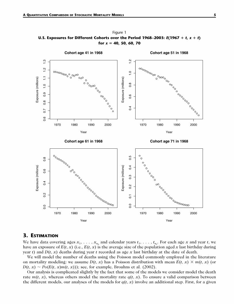
A QUANTITATIVE COMPARISON OF STOCHASTIC MORTALITY MODELS 5
Figure 1U.S. Exposures for Different Cohorts over the Period 1968–2003: E(1967 � t, x � t)
for x � 40, 50, 60, 70
1970 1980 1990 2000
0.6
0.7
0.8
0.9
1.0
1.1
1.2
1.3
Cohort age 41 in 1968
Year
Exp
osur
e (m
illio
ns)
1970 1980 1990 2000
0.4
0.6
0.8
1.0
1.2
Cohort age 51 in 1968
Year
Exp
osur
e (m
illio
ns)
1970 1980 1990 2000
0.0
0.2
0.4
0.6
0.8
Cohort age 61 in 1968
Year
Exp
osur
e (m
illio
ns)
1970 1980 1990 2000
0.0
0.1
0.2
0.3
0.4
0.5
Cohort age 71 in 1968
Year
Exp
osur
e (m
illio
ns)
3. ESTIMATION
We have data covering ages x1, . . . , and calendar years t1, . . . , For each age x and year t, wex t .n na y
have an exposure of E(t, x) (i.e., E(t, x) is the average size of the population aged x last birthday duringyear t) and D(t, x) deaths during year t recorded as age x last birthday at the date of death.
We will model the number of deaths using the Poisson model commonly employed in the literatureon mortality modeling: we assume D(t, x) has a Poisson distribution with mean E(t, x) � m(t, x) (orD(t, x) � Po(E(t, x)m(t, x))); see, for example, Brouhns et al. (2002).
Our analysis is complicated slightly by the fact that some of the models we consider model the deathrate m(t, x), whereas others model the mortality rate q(t, x). To ensure a valid comparison betweenthe different models, our analyses of the models for q(t, x) involve an additional step. First, for a given

6 NORTH AMERICAN ACTUARIAL JOURNAL, VOLUME 13, NUMBER 1
Table 1Formulae for the Mortality Models
Model Formula
M1 log m(t, x) � �(1) (2) (2)� � �x x t
M2 log m(t, x) � � �(1) (2) (2) (3) (3)� � � � �x x t x t�x
M3 log m(t, x) � � �(1) �1 (2) �1 (3)� n � n �x a t a t�x
M4 log m(t, x) � �i, j�i j (x, t)ayBi j
M5 logit q(t, x) � � (x �(1) (2)� � x)t t
M6 logit q(t, x) � � (x � �(1) (2) (3)� � x) �t t t�x
M7 logit q(t, x) � � (x � � ((x � 2 � �(1) (2) (3) 2 (4)� � x) � x) � ) �ˆt t t x t�x
M8 logit q(t, x) � � (x � � (xc �x)(1) (2) (3)� � x) �t t t�x
Notes: The functions and are age, period, and cohort effects, respectively. The (x, t) are B-spline basis functions, and the �i j are(i) (i) (i) ay� , � , � Bx t t�x i jweights attached to each basis function. na is the number of ages covered; is the mean age over the range of ages being used in the analysis;x
is the mean value of (x �2 2� x) .ˆx
set of parameters, we calculate the q(t, x). We then transform these into death rates using the identitym(t, x) � �log[1 � q(t, x)]. We can now calculate the likelihood for all models consistently based onthe m(t, x) values.
For a given model we use to represent the full set of parameters, and the notation for m(t, x) isaugmented to read m(t, x; ) to indicate its dependence on these parameters. Where we have a modelfor q(t, x) � q(t, x; ) we define
m(t, x; ) � �log[1 � q(t, x; )].
For all models the log-likelihood is
l(; D, E) � D(t, x) log[E(t, x)m(t, x; )] � E(t, x)m(t, x; ) � log[D(t, x)!],�t,x
and estimation is by maximum likelihood.8
4. THE MORTALITY MODELS
The data will cover the range x1, . . . , and t1, . . . , with unit increments in each case. Modelsx tn na y
will be labeled M1, M2, etc., and are listed in Table 1. Additionally we will use the following conventions:
• The functions will reflect age-related effects.(i)�x
• The functions will reflect period-related effects.(i)�t
• The functions will reflect cohort-related effects, with c � t � x.(i)�c
All of the models that we examine, with the exception of the P-splines model, will be of the form logm(t, x) � �i or logit q(t, x) � �i
(i) (i) (i) (i) (i) (i)� � � � � � .x t t�x x t t�x
The method of recording the calendar year of death and the age last birthday at death means thatthe death count covers individuals born on January 1 in calendar year t � x � 1 through to December31 t � x (i.e., two years). The cohort index c � t � x takes its values from the second of these years.To illustrate, the 1886 cohort discussed above in Section 2.1 covers individuals born between January1, 1885 and December 31, 1886.
4.1 Model M1Lee and Carter (1992) propose the following model for death rates:
(1) (2) (2)log m(t, x) � � � � � .x x t
8 Note that D(t, x)! means ‘‘D(t, x) factorial.’’

A QUANTITATIVE COMPARISON OF STOCHASTIC MORTALITY MODELS 7
For this and some of the other models, there is an identifiability problem in parameter estimation. Tosee this, note that the revised parameterization
(1) (2) (2)˜ ˜log m(t, x) � � � � � ,˜x x t
where
(1) (1) (2)� � � � b� ,x x x
(2) (2)� � � /a,x x
(2) (2)� � a(� � b)˜t t
results in identical values for log m(t, x), and this means that we cannot distinguish between the twoparameterizations. To circumvent this we need to impose two constraints on the parameters. To someextent the choice of constraints is a subjective one, although some choices are more natural thanothers. With the current model we use the following constraints:
(2)� � 0,� tt
(2)� � 1.� xx
The first is a natural constraint and implies that, for each x, the estimate for will be equal (at(1)�x
least approximately) to the mean over t of the log m(t, x). There also has to be a second constraint topin down unique values of parameters a and b above. However, there is no natural choice for this, and,indeed, different choices can be seen in different applications of the Lee-Carter model in the academicliterature. The important point to note, however, is that the choice of the second constraint has noimpact on either the quality of the fit or on the forecasts of mortality.
4.2 Model M2Renshaw and Haberman (2006) generalized the Lee-Carter model to include a cohort effect as follows:
(1) (2) (2) (3) (3)log m(t, x) � � � � � � � � .x x t x t�x
Model M1 is then a special case where the and are set to zero.(3) (3)� �x t�x
This model has similar identifiability problems as the previous model. We therefore impose the fol-lowing constraints to ensure identifiability:
(2)� � 0,� tt
(2)� � 1,� xx
(3)� � 0,� t�xx,t
(3)� � 1. (4.1)� xx
The first and third constraints mean that the estimate for will be (at least approximately) equal(1)�x
to the mean over t of the log m(t, x). The second and fourth constraints are similar to the secondconstraint in model M1, in that there are no natural choices, although the actual choice makes nodifference to the quality of fit.
The original RH (2006) study chose to fix estimates for at �t log m(t, x); the remaining(1) �1� nx y
parameters were estimated using an iterative process. In contrast, we use RH’s estimate for only(1)�x
as a starting value and include in the iterative scheme as well.(1)�x

8 NORTH AMERICAN ACTUARIAL JOURNAL, VOLUME 13, NUMBER 1
We found that parameter values converge very slowly to their maximum likelihood estimates. Thissuggests that an identifiability problem remains. It is not clear if this problem is an exact one or anapproximate one. An exact identifiability problem means that the likelihood function will be absolutelyflat in certain dimensions, whereas an approximate identifiability problem means that the likelihoodfunction will be close to flat in certain dimensions.
4.3 Model M3Currie (2006) introduces the simpler Age-Period-Cohort (APC) model
1 1(1) (2) (3)log m(t, x) � � � � � � ,x t t�xn na a
where na is the number of ages in the dataset. The APC model has its origins in medical statistics andpredates the Lee-Carter model (see, e.g., Osmond 1985; Jacobsen et al. 2002). The model is also aspecial case of model M2 with � 1/na and � 1/na. Currie (2006) uses P-splines to fit(2) (3) (1)� � � ,x x x
and to ensure smoothness, although the method is approximate. In our analysis of M3, we do(2) (3)� , �t t�x
not impose any smoothness conditions.9
Without loss of generality, we impose the following constraints:(2)� � 0,� t
t
(3)� � 0.� t�xx,t
We need one further constraint, because we can otherwise add ((t � � (x � to subtract(3)t) x)) � ,t�x
(t � from and add (x � to with no impact on the two constraints above. We propose(2) (1)t) � , x) �t x
here that the tilting parameter, , be chosen within an iterative scheme to minimize(1) (1) 2¯S() � (� � (x � x) � � ) ,� x x
x
where � �t log m(t, x). This implies that(1) �1� nx y
(1) (1)¯� (x � x)(� � � )x x x � � .2� (x � x)x
Given that the and already satisfy the first two constraints, we revise our parameter estimates(2) (3)� �t t�x
according to the following formulas:(2) (2) ¯� � � � n (t � t),˜t t a
(3) (3) ¯� � � � n ((t � t) � x � x)),˜t�x t�x a
(1) (1)� � � � (x � x).x x
Note that models M1 to M3 can be described as belonging to the family of generalized Lee-Cartermodels.
4.4 Model M4Currie, Durban, and Eilers (2004) propose the use of B-splines and P-splines to fit the mortality surface:
aylog m(t, x) � � B (x, t),� i j i ji, j
9 Although we use the same model, Currie (2006) incorporates a penalty for lack of smoothness. As a result, estimates for the three functionswill be different.

A QUANTITATIVE COMPARISON OF STOCHASTIC MORTALITY MODELS 9
with smoothing of the �i j in the age and cohort directions. Currie also discuss the construction of B-splines and how they are fitted.
4.5 Model M5M5 is the original CBD model. CBD (2006b) fitted the following model to mortality rates q(t, x):
[q(t, x) (1) (1) (2) (2)logit q(t, x) � log � � � � � � .� � x t x t(1 � q(t, x))
For this model simple parametric forms were assumed for and(1) (2)� � :x x
(1)� � 1,x
(2)� � (x � x),x
where � �ixi is the mean age in the sample range (in our analysis, therefore, � 74.5). Thus,�1x n xa
(1) (2)logit q(t, x) � � � � (x � x).t t
This model has no identifiability problems.
4.6 Model M6This model is the first generalization of the CBD model to include a cohort effect:
(1) (1) (2) (2) (3) (3)logit q(t, x) � � � � � � � � � .x t x t x t�x
For this model simple parametric forms were assumed for and(1) (2) (3)� , � , � :x x x
(1)� � 1,x
(2)� � (x � x),x
(3)� � 1.x
Thus,(1) (2) (3)logit q(t, x) � � � � (x � x) � � .t t t�x
As with other models, we have an identifiability problem. Here we can switch from to �(3) (3)� �t�x t�x
� 1 � 2(t � x � and, with corresponding adjustments to and there is no impact(3) (1) (2)� x), � � ,t�x t t
on the fitted values of the q(t, x). This requires two constraints to prevent arbitrary use of 1 and 2.The constraints we have used here are
(3)� � 0,� cc�C
(3)c� � 0,� cc�C
where the C is the set of cohort years of birth that have been included in the analysis (see Section2.1). The reason for this choice is that if we use least squares to fit a linear function 1 � 2c to
the constraints ensure that � 0 and � 0. This ensures that the fitted will fluctuate(3) (3)ˆ ˆ� , �c 1 2 c
around 0 and will have no discernible linear trend.
4.7 Model M7This model is a generalization of model M6 that adds a quadratic term to the age effect. The inclusionof the quadratic term is inspired by the possible curvature identified in the logit q(t, x) plots in theU.S. data. Thus,

10 NORTH AMERICAN ACTUARIAL JOURNAL, VOLUME 13, NUMBER 1
(1) (2) (3) 2 2 (4)logit q(t, x) � � � � (x � x) � � ((x � x) � � ) � � .ˆt t t x t�x
Here the constant � �i(x � is the mean of (x �2 �1 2 2� n x) x) .ˆx a
As with model M6, we have an identifiability problem, and we can switch from to � �(4) (4) (4)� � �˜t�x t�x t�x
1 � 2(t � x � � 3(t � x � and corresponding adjustments to and without2 (1) (2) (3)x) x) � , � , � ,t t t
there being an impact on the fitted values of the q(t, x). This requires three constraints to preventarbitrary choices over 1, 2, and 3. The constraints we have used here are
(4)� � 0,� cc�C
(4)c� � 0,� cc�C
2 (4)c � � 0.� cc�C
Thus, if we use least squares to fit a quadratic function 1 � 2c � 3c2 to the constraints ensure(4)� ,c
that � 0, � 0 and � 0, meaning that the fitted will fluctuate around 0 and will have no(4)ˆ ˆ ˆ �1 2 3 c
discernible linear trend or quadratic curvature.
4.8 Model M8Our third generalization of the CBD model builds on our experience from fitting model M2 (see theresults in Section 6). This suggested that the impact of the cohort effect for any specific cohort(3)�c
diminishes over time (i.e., is decreasing with x) instead of remaining constant (i.e., is constant).(3) (3)� �x x
This leads to(1) (1) (2) (2) (3) (3)logit q(t, x) � � � � � � � � � ,x t x t x t�x
where(1)� � 1,x
(2)� � (x � x),x
(3)� � (x � x)x c
for some constant parameter xc to be estimated. This results in(1) (2) (3)logit q(t, x) � � � � (x � x) � � (x � x).t t t�x c
To avoid identifiability problems, we need to introduce one constraint:(3)� � 0.� t�x
x,t
Each of models M6–M8 is an extension of model M5 with some allowance for the cohort effect.Consequently models M5–M8 can be described as members of the family of generalized CBD-Perksmodels.
4.9 Philosophical Similarities and Differences between ModelsWe comment here briefly on the philosophical similarities and differences behind the structural as-sumptions of the models. The reader can use these to help form preferences over the models in thecase where quantitative and qualitative criteria do not permit a clear-cut distinction between them.
All the models M1–M3 and M5–M8 share the same underlying assumption that the age, period, andcohort effects are qualitatively different in nature and hence need to be modeled in different ways.Specifically they recognize a randomness in mortality rates at each age from one year to the next,perhaps caused by local environmental factors (such as a winter influenza outbreak or a summer heat-

A QUANTITATIVE COMPARISON OF STOCHASTIC MORTALITY MODELS 11
Table 2Desirable Model Properties
Model M1 M2 M3 M4 M5 M6 M7 M8
Parsimony ? ? ? ? ? ? ? ?Transparency ? ? ? ? ? ? ? ?Ability to generate sample paths Y Y Y N Y Y Y YIncorporation of cohort effects N Y Y Y N Y Y YNontrivial correlation structure N N? N? N Y Y Y Y
Notes: The table shows whether each model satisfies each of the stated criteria. Where a criterion cannot be answered with a simple Y(es) orN(o), the question mark indicates that the model lies somewhere in the middle, with further comments in the main text.
Table 3England and Wales Males Aged 60–89 and
Years 1961–2004
ModelMaximum
Log-LikelihoodEffective Number
of Parameters BIC (Rank)
M1 �8,912.7 102 �9,275.8 (6)M2 �7,735.6 203 �8,458.1 (3)M3 �8,608.1 144 �9,120.6 (5)M4 �9,245.9 74.2 �9,372.9 (7)M5 �10,035.5 88 �10,348.8 (8)M6 �7,922.3 159 �8,488.3 (4)M7 �7,702.1 202 �8,421.1 (2)M8 �7,823.7 161 �8,396.8 (1)
Notes: Maximum likelihood, effective number of parameters esti-mated, and Bayes Information Criterion (BIC) for each model. Theeffective number of parameters takes account of the constraints onparameters or the effect of the penalty functions in the case of modelM4. For M4 with dx � 4 and dt � 4 interknot distances, the BIC isoptimized over the penalty weights.
wave), which is not observed between adjacent ages. In contrast, the P-splines model, M4, assumes thatthere is smoothness in the underlying mortality surface in the period effects as well as in the age andcohort effects. Models M5–M8 differ from M1–M3 in that the former assume a functional relationship(and hence smoothness) between mortality rates over adjacent ages within the same year.
Depending on one’s personal beliefs about the underlying randomness in the age, period, and cohorteffects, one might attach greater weight to models that are aligned with these beliefs. For example, ifone believes that there should be an underlying smoothness in mortality rates between adjacent ageswithin the same year, that there is randomness in mortality rates between cohorts, and randomness inmortality rates from one year to the next, then greater weight might be placed on models M6–M8.
5. ALTERNATIVE WAYS OF EVALUATING AND COMPARING MORTALITY MODELS
We can evaluate and compare the eight models using a range of criteria.
5.1 Desirable Properties of the Theoretical ModelsFirst, we can compare the main features of the models against a set of desirable model properties aslisted below and derived from CMI (2005, 2006) and Cairns, Blake, and Dowd (2006a). Table 2 assesseseach model against these properties:
• Parsimony: Other things being equal, a model with fewer parameters is preferable to a model withmore. Each of the models has a large number of parameters (see Table 3), so none could be describedas parsimonious in any absolute sense. However, some models are more parsimonious than others,having fewer parameters.

12 NORTH AMERICAN ACTUARIAL JOURNAL, VOLUME 13, NUMBER 1
Of course, other things are not equal including the value of the maximum likelihood, and so abalance between statistical goodness of fit and parsimony is achieved through the use of the BayesInformation Criterion (see Section 6.1.1).
In Table 2 we have placed question marks next to all eight models in respect to parsimony. Torecord a ‘‘N(o)’’ would indicate that a model was unnecessarily complex, which we do not think isthe case with any model, whereas a ‘‘Y(es)’’ would indicate that a model had a small number ofparameters, which is also not the case with any model.
• Transparency: How much of the model and its output is treated as a ‘‘black box’’? It is importantthat the user of a given model understands the model and all of its workings, to avoid the dangerthat the model might be used inappropriately. At the same time, a model that is transparent to oneperson might not be transparent to someone else. Thus, rather than impose our own judgementshere, we leave question marks next to all models.
• Whether the model has the ability to generate sample paths:10 The process uncertainty that generatesrandom sample paths is necessary for tasks such as pricing longevity-linked financial instruments anddeveloping related hedging strategies (see, e.g., Blake et al. 2006). Only the P-splines model, M4,fails on this criterion. M4 assumes that there is an underlying smoothness to the mortality surfaceand that the only uncertainty in forecasts (which can be substantial) is due to model and parameteruncertainty.
• Incorporation of cohort effects: This is important if we believe that cohort effects are present andneed to be allowed for (as discussed in Section 2.1).
• Ability to produce a nontrivial correlation structure between the year-on-year changes in mortalityrates at different ages.11 The correlation structure is described as trivial when there is perfect cor-relation between changes in mortality rates at different ages from one year to the next. This is thecase for model M1, for example, where there is a single time series process For models M2 and(2)� .t
M3, we also have perfect correlation (for the same reason) at all ages except at the youngest age,where there is potentially additional randomness arising from the arrival of a new cohort with anunknown cohort effect. Models M5–M8 allow for a nontrivial correlation structure because they allhave more than one underlying period risk factor.
5.2 Desirable Properties of the Fitted ModelsImportant additional properties can be evaluated only when we fit the model to the data:
• A good model should provide a good fit to the historical data, produce testable predictions that areconsistent with the data, and rank well against other models by criteria such as the BIC.
• Parameter estimates should be robust relative to the range of data employed. For example, if we useEW data for 1981–2004, we would hope to see similar parameter estimates to those found using datafor 1961–2004.
• Where a model is used for forecasting future rates of mortality, individual scenarios should exhibit‘‘biologically reasonable’’ behavior. For example, forecast mortality rates should both be increasingin age in any given forecast year and change smoothly over time (see, e.g., Cairns, Blake, and Dowd2006a). The quantitative and qualitative forecasting properties of models are considered only brieflyin this paper (Sections 6.3 and 7.3). These issues are considered in detail elsewhere (Cairns et al.2008; Dowd et al. 2008a,b).
10 We refer here to sample paths for the underlying (and unobservable) death rates m(t, x). A different type of sample path can be constructedwhen we look at crude (observable) death rates under the Poisson model: m(t, x) � D(t, x)/E(t, x), where D(t, x) � Po(m(t, x)E(t, x)).11 Statistical analysis of mortality rates points to changes in the m(t, x) at different ages being imperfectly correlated. The existence of anontrivial correlation structure implies, for example, that hedging of longevity-linked liabilities, such as annuities, requires more than onehedging instrument. See also Cairns, Blake, and Dowd (2008) for further discussion of the evidence for imperfect correlation.

A QUANTITATIVE COMPARISON OF STOCHASTIC MORTALITY MODELS 13
6. ANALYSIS OF MODELS USING ENGLAND AND WALES DATA
6.1 Model Selection CriteriaIn this section we conduct formal model comparisons based on England and Wales data. For eachmodel we estimate (as appropriate) the and for each factor, i, age, x, year, t, and cohort,(i) (i) (i)� , � , �x t c
c � t � x, by maximizing the log-likelihood function. Estimates of the and are plotted in(i) (i) (i)� , � , �x t c
Figures 3–9.Values for the maximum likelihood, effective number of parameters (or degrees of freedom in esti-
mation), and the Bayes Information Criterion (BIC) for each model are given in Table 3.
6.1.1 Bayes Information CriterionIf one simply compares the maximum likelihoods attained by each model, then it is natural for modelswith more parameters to fit the data ‘‘better.’’ Such improvements are almost guaranteed if modelsare nested: if one model is a special case of another, then the model with more parameters will typicallyhave a higher maximum likelihood, even if the true model is the model with fewer parameters.
To avoid this problem, we need to penalize models that are overparameterized. Specifically, for eachparameter that we add to a model, we need to see a ‘‘significant’’ improvement in the maximumlikelihood rather than just an increase of any size. A number of such penalties have been proposed.Here we focus on the Bayes Information Criterion (BIC; see, e.g., Hayashi 2000; Cairns 2000).
A key point about the use of the BIC is that it provides us with a mechanism for striking a balancebetween quality of fit (which can be improved by adding in more parameters) and parsimony. A second,and equally important point about the BIC, is that it allows us to compare models that are not nec-essarily nested. For example, M1 and M3 are nested within M2, but M1 is not nested within M3 andvice versa. A final point is that the BIC makes no assumptions about ‘‘prior’’ model rankings: that is,all models have equal status in terms of how we rank them. In contrast, hypothesis tests start from anull hypothesis that favors one specific model over the others.
The BIC for model r is defined as12
1ˆBIC � l( ) � � log N,r r r2where r is the parameter vector for model r, is its maximum likelihood estimate, l is theˆ ˆ ( )r r
maximum log likelihood, N is the number of observations (not counting those cells that have beenexcluded from the analysis), and �r is the effective number of parameters being estimated.13
The models can then be ranked, with the top model having the highest BIC. Values for the BIC aregiven in Table 3, and we see that model M8 comes out on top in the BIC rankings with M7 second.14
6.1.2 Standardized ResidualsA second model selection criterion relates to the standardized residuals:
ˆD(t, x) � E(t, x)m(t, x; )ˆZ(t, x) � . (6.1)� ˆE(t, x)m(t, x; )ˆ
Embedded within our modeling hypothesis is an assumption that the death counts are independentPoisson random variables for each age and year (Section 3). If our hypothesis is true, therefore, the
12 Some authors define the BIC as �2l � �r log N: that is, �2 times our definition. The two definitions are equivalent and have no impactˆ( )ron our analysis.13 For example, model M1 requires estimates for 30 values of 30 values of and 44 values of totaling 104, but we then deduct 2(1) (2) (2)� , � , � ,x x t
from this total to reflect the two constraints �t � 0 and �x � 1. For the P-splines model the concept of the effective number of(2) (2)� �t x
parameters is more abstract; see Currie, Durban, and Eilers (2004) and references therein for further details.14 This is no accident. We searched across a range of new functional forms to achieve this outcome (see also note 1).

14 NORTH AMERICAN ACTUARIAL JOURNAL, VOLUME 13, NUMBER 1
Table 4Sample Variances of Standardized Residuals
for Models M1–M8
Model
M1 M2 M3 M4 M5 M6 M7 M8
Var [Z(t, x)] 4.1 2.2 3.7 4.3 5.9 2.4 2.1 2.3
standardized residuals (eq. [6.1]) will be approximately i.i.d. standard normal random variables.Models that have higher likelihood have a lower variance of the standardized residuals. However, for
each model discussed in this paper, the variance of the standardized residuals is significantly greaterthan one (see Table 4). This ‘‘overdispersion’’ seems to be a general feature of mortality data in manycountries. A possible source of this overdispersion lies in the fact that the exposures data are estimated.We conjecture that this overdispersion does not have a significant impact on our estimates of thefuture dynamics of the underlying mortality rates q(t, x). Nevertheless, a Poisson model might under-estimate the future variability of the actual death rates relative to the true underlying rates.
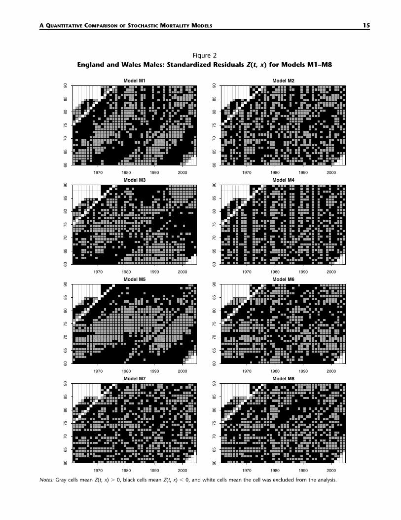
A simple means of considering the validity of the i.i.d. assumption of the Z(t, x) is to look at thepattern of positive and negative standardized residuals (see Koissi, Shapiro, and Hognas 2006): thepattern should be random under the i.i.d. hypothesis. For models M1, M3, and M5 (see Fig. 2), theplots of the residuals show a strong clustering of positives and negatives. Models M1 and M5 do notincorporate a cohort effect, and there are diagonal clusters of positive and negative residuals: thisprovides strong evidence for the existence of a cohort effect. M6 also shows some clustering, but muchless than M1, M3, and M5. The standardized residuals in M4, at first glance, look reasonably random,but closer inspection reveals distinct vertical bands that suggest that there is a genuine random periodeffect that is being smoothed out too much under M4. M2, M7, and M8 all look reasonably random,and so all pass the test on a visual inspection.15
6.1.3 Comparison of Nested ModelsSome models are nested within one of the others: that is, they are special cases of more general models.For example, model M1 is nested within model M2, being a special case of M2 with � 0 for all x,(3)�x
and � 0 for all c � t � x. In such circumstances we can use the likelihood ratio test to test the(3)�c
null hypothesis that the nested or restricted model is the correct model versus the alternative hypoth-esis that the more general model is correct. For the nested model, let be the maximum log likelihoodl1
for model M1 and be the maximum likelihood for model M2. Model M1 requires the estimation ofl2
�1 � 102 parameters, while M2 requires �2 � 203. The likelihood-ratio test statistic is 2( � Ifˆ ˆl l ).2 1
the null hypothesis is true, this should have approximately a chi-squared distribution with �2 � �1
degrees of freedom (d.f.). Thus we reject the null hypothesis in favor of the more general model if thetest statistic is too large: specifically, if 2( � ) � where � is the significance level. Alter-2ˆ ˆl l ,2 1 � �� ,�2 1
natively, we can calculate the p-value for this test as p � 1 � �1(2( � )).2 ˆ ˆ l l� �� 2 12 1
The eight models considered here include seven nested pairs. Each pair is considered in Table 5. Ineach case, the null hypothesis is rejected overwhelmingly in favor of the more general model. Theseresults support our earlier findings based on the BIC. Additionally, the decisive rejection of models M1and M5, in particular, gives a clear indication that the cohort effect is a key feature of EW malesmortality data.
15 Complementing these plots, one can plot standardized residuals against age, year of observation, and year of birth as in RH (2006). We donot include such plots here, but simply note that these plots reveal the same information, but in different ways, to Table 4 and Figure 2.
A QUANTITATIVE COMPARISON OF STOCHASTIC MORTALITY MODELS 15
Figure 2England and Wales Males: Standardized Residuals Z(t, x) for Models M1–M8
1970 1980 1990 2000
6065
7075
8085
90
Model M1
1970 1980 1990 2000
6065
7075
8085
90
Model M2
1970 1980 1990 2000
6065
7075
8085
90
Model M3
1970 1980 1990 2000
6065
7075
8085
90
Model M4
1970 1980 1990 2000
6065
7075
8085
90
Model M5
1970 1980 1990 2000
6065
7075
8085
90
Model M6
1970 1980 1990 2000
6065
7075
8085
90
Model M7
1970 1980 1990 2000
6065
7075
8085
90
Model M8
Notes: Gray cells mean Z(t, x) � 0, black cells mean Z(t, x) � 0, and white cells mean the cell was excluded from the analysis.

16 NORTH AMERICAN ACTUARIAL JOURNAL, VOLUME 13, NUMBER 1
Table 5England and Wales Data: Likelihood Ratio Test Results for Various Pairs of General
and Nested Models
H0: Restricted Model H1: General Model LR Test Statistic d.f. p-Value
M1M3M5M5M6M5M6
M2M2M6M7M7M8M8
2,354.31,745.04,226.54,666.8
440.34,423.7
197.2
1015971
11443742
�0.000001�0.000001�0.000001�0.000001�0.000001�0.000001�0.000001
6.2 Parameter Estimates and Their RobustnessIn Figures 3–9, we have plotted the maximum-likelihood estimates for the various parameters in allmodels, except M4, using EW males data, aged 60–89.16 In this section we will focus on the parameter
Figure 3England and Wales Data: Parameter Estimates for Model M1
60 65 70 75 80 85 90
–5–4
–3–2
–1
Beta_1(x)
Age, x
60 65 70 75 80 85 90
0.00
0.01
0.02
0.03
0.04
0.05
Beta_2(x)
Age, x
1960 1970 1980 1990 2000
–20
–10
010
20
Kappa_2(t)
Year, t
Notes: Derived from (a) data from 1961–2004 (dots) or (b) data from 1981–2004 (solid lines).
16 See Section 2.1 for exclusions.
A QUANTITATIVE COMPARISON OF STOCHASTIC MORTALITY MODELS 17
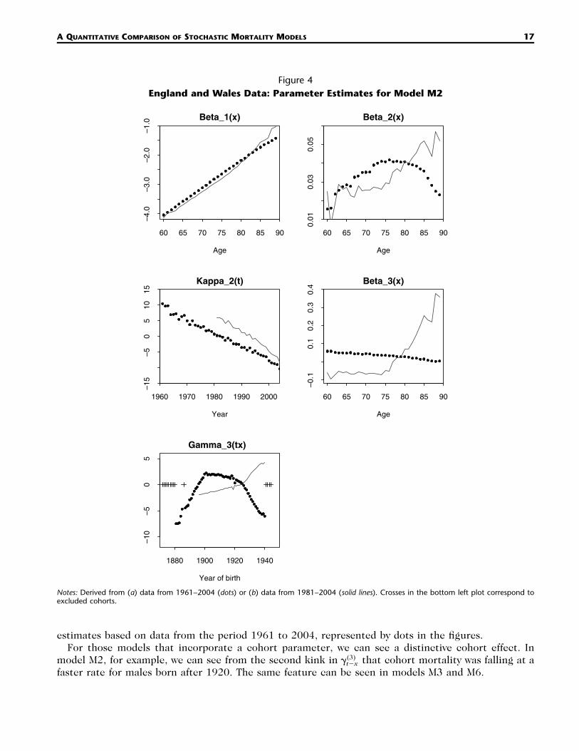
Figure 4England and Wales Data: Parameter Estimates for Model M2
60 65 70 75 80 85 90
–4.0
–3.0
–2.0
–1.0
Beta_1(x)
Age
60 65 70 75 80 85 90
0.01
0.03
0.05
Beta_2(x)
Age
1960 1970 1980 1990 2000
–15
–50
510
15
Kappa_2(t)
Year
60 65 70 75 80 85 90
–0.1
0.1
0.2
0.3
0.4
Beta_3(x)
Age
1880 1900 1920 1940
–10
–50
5
Gamma_3(tx)
Year of birth
Notes: Derived from (a) data from 1961–2004 (dots) or (b) data from 1981–2004 (solid lines). Crosses in the bottom left plot correspond toexcluded cohorts.
estimates based on data from the period 1961 to 2004, represented by dots in the figures.For those models that incorporate a cohort parameter, we can see a distinctive cohort effect. In
model M2, for example, we can see from the second kink in that cohort mortality was falling at a(3)�t�x
faster rate for males born after 1920. The same feature can be seen in models M3 and M6.

18 NORTH AMERICAN ACTUARIAL JOURNAL, VOLUME 13, NUMBER 1
Figure 5England and Wales Data: Parameter Estimates for Model M3
60 65 70 75 80 85 90
–5–4
–3–2
–1
Beta_1(x)
Age, x
1960 1970 1980 1990 2000
–10
–50
510
Kappa_2(t)
Year, t
1880 1900 1920 1940
–8–6
–4–2
02
Gamma_3(t)
Year, t
Notes: Derived from (a) data from 1961–2004 (dots) or (b) data from 1981–2004 (solid lines). Crosses in the bottom left plot correspond toexcluded cohorts. � and �(2) 1 (3) 1–– ––� � .x 30 x 30
For models M7 and M8, the cohort effect follows a different pattern. In M7 part of the cohort effecthas been substituted by the additional quadratic age effect. The M8 cohort effect seems to follow asimilar pattern except for the fact that it has been tilted slightly.
6.2.1 RobustnessAn important property of a model is the robustness of its parameter estimates relative to changes inthe period of data used to fit a given model.
For each model, except M4, we have plotted (Figs. 3–9) parameter estimates based on data from1961 to 2004 (represented by dots) and from 1981 to 2004 (solid lines). We focus our comments hereon the four highest BIC-ranked models M2, M6, M7, and M8. The plots reveal that, out of the fourmodels, M7 seems to be the most robust relative to changes in the period of data used: that is, theparameter estimates hardly change even when we use a much shorter data period.
M2, on the other hand, seems to produce results that lack robustness, because the parameter esti-mates jump to a qualitatively quite different solution when we use less data. For example, consider the
plot in Figure 4. Here is strictly positive and declining when we use data from 1961 to 2004.(3) (3)� �x x
In contrast, for the 1981–2004 data, is flat and negative initially, but then becomes positive and(3)�x

A QUANTITATIVE COMPARISON OF STOCHASTIC MORTALITY MODELS 19
Figure 6England and Wales Data: Parameter Estimates for Model M5
1960 1970 1980 1990 2000
–3.2
–3.0
–2.8
–2.6
–2.4
Kappa_1(t)
Year, t
1960 1970 1980 1990 2000
0.08
0.09
0.10
0.11
0.12
Kappa_2(t)
Year, t
Notes: Derived from (a) data from 1961–2004 (dots) or (b) data from 1981–2004 (solid lines). � 1 and � x �(1) (2)� � x.x x
increases steeply: a shape that cannot, qualitatively, be reconciled (e.g., by changing the identifiabilityconstraint, eq. [4.1]) with the 1961–2004 shape for This lack of robustness brings into question(3)� .x
the reliability of any projections made using M2. Reinforcing this concern, CMI (2007, Section 7)observed a similar lack of robustness in M2 when different age ranges are used.
M8 appears reasonably robust, and the differences that we do see are, in fact, consequences of theconstraint that � 0 when we are summing over different years. However, we did find that, for(3)� �t,x t�x
some datasets, the M8 fitting program was very slow to converge. We found a similar problem with M2and put this down to the possible existence of multiple maxima in the likelihood function and theconsequential risk of parameter instability. In our extensive testing, we found no such problems withM1, M3, M5, M6, or M7. M6 also appears reasonably robust, and again the bigger differences that wesee are due to the identifiability constraints being applied over a different range of years.
The question of robustness is explored further and at length elsewhere (Cairns et al. 2008; Dowd etal. 2008a,b).
6.3 Model Forecasting PropertiesWe will now carry out a number of tests to assess the impact of model choice on key outputs associatedwith projections of mortality rates into the future. We focus, for illustrative purposes, on models M2,M6, M7, and M8: these are the four top-ranked models for the EW males dataset (Table 3).
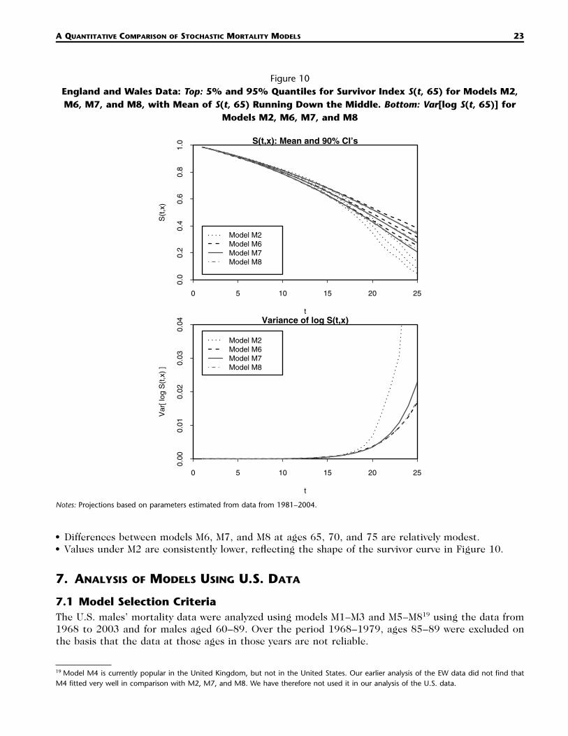
6.3.1 Survivor Index ProjectionsWe first consider the impact of model choice on projected values of the survivor index S(t, 65): theproportion out of the cohort aged 65 (and still alive) in 2004 who are still alive in year 2004 � t.17 InFigure 10 (top), we have plotted the mean and 90% prediction interval for the survivor index S(t, 65)for a cohort aged 65 in 2004. It can be seen that these forecasts are little affected by the choicebetween models M7 and M8. M6 is slightly different, but consistent with M7 and M8. M2 is more outof line. This is connected to the qualitatively different shape of the parameter estimates under M2
17 Projections are based on parameters fitted to data from 1981 to 2004 and use a multivariate random walk model in simulations based onthe historical estimates of the Further details are given in the Appendix.(i)� .t

20 NORTH AMERICAN ACTUARIAL JOURNAL, VOLUME 13, NUMBER 1
Figure 7England and Wales Data: Parameter Estimates for Model M6
1960 1970 1980 1990 2000
–3.4
–3.0
–2.6
–2.2
Kappa_1(t)
Year, t
1960 1970 1980 1990 2000
0.08
0.09
0.10
0.11
0.12
Kappa_2(t)
Year, t
1880 1900 1920 1940
–0.2
0–0
.10
0.00
0.10
Gamma_3(t)
Year, t
Notes: Derived from (a) data from 1961–2004 (dots) or (b) data from 1981–2004 (solid lines). Crosses in the bottom left plot correspond toexcluded cohorts. � 1, � x � and � 1.(1) (2) (3)� � x, �x x x
using data from 1981 to 2004 versus those using data from 1961 to 2004 (Fig. 4). Figure 11 comparesprojections of the survivor index for M2 using data from 1961 to 2004 (dashed lines)18 and 1981 to2004 (dotted lines). The former is much closer to the projections under M6, M7, and M8 in Figure 10,and the substantial differences reinforce the concern expressed in Section 6.2.1 that M2 is not robust.
In Figure 10 (bottom) we have plotted the variance of log S(t, 65) over time. Again the differencesare relatively small between M6, M7, and M8, although some differences emerge close to 25 years. M2(1981–2004 data) stands out as having a much higher variance, suggesting that model risk might bean issue. A possible implication is that the choice of model might have a significant effect on quantitiesthat rely, to some extent, on the variance of S(t, x). For example, the price of a financial option thathas S(t, x) as its underlying quantity is strongly dependent on the variance of S(t, x): everything elsebeing equal, the higher the variance, the higher the value of the option.
We have concentrated here on the contribution of model risk to forecast uncertainty. However, it isappropriate to allow for parameter uncertainty to provide a more complete picture of the level of risk
18 M2 is fitted to data from 1961 to 2004, but for greater consistency with the 1981–2004 data projections are based on the last 24 observationsof and the last 45 observations of(2) (3)� � .t c

A QUANTITATIVE COMPARISON OF STOCHASTIC MORTALITY MODELS 21
Figure 8England and Wales Data: Parameter Estimates for Model M7
1960 1970 1980 1990 2000
–3.2
–3.0
–2.8
–2.6
–2.4
Kappa_1(t)
Year
1960 1970 1980 1990 2000
0.08
00.
090
0.10
00.
110
Kappa_2(t)
Year
1960 1970 1980 1990 2000–1 e
-03
–4 e
-04
2 e
-04
Kappa_3(t)
Year
1880 1900 1920 1940
–0.0
6–0
.02
0.02
0.06
Gamma_4(t–x)
Year of birth
Notes: Derived from (a) data from 1961–2004 (dots) or (b) data from 1981–2004 (solid lines). Crosses in the bottom right plot correspond toexcluded cohorts. � 1, � x � � (x � )2 � and � 1.(1) (2) (3) 2 (4)� � x, � x � , �ˆx x x x x
associated with, for example, future longevity-linked cash flows. The impact of parameter uncertaintyis explored in more depth by Czado, Delwarde, and Denuit (2005), Cairns, Blake, and Dowd (2006b),and Dowd, Cairns, and Blake (2006), who take Bayesian approaches, and Koissi, Shapiro, and Hognas(2006) and CMI (2005), who use a bootstrapping methodology. These analyses suggest that parameteruncertainty can significantly increase the overall level of measured uncertainty, particularly for moredistant longevity-linked cash flows.
6.3.2 Projecting Annuity ValuesAs a second projection exercise, we calculated the value in 2004 of an annuity payable until age 90(the maximum age in our projection model) for males aged 60, 65, 70, and 75 in 2004 at a constantinterest rate of 4% p.a.:
90�x�0.04ta (2004) � e E[S(t, x)].�x
t�1
Projections of S(t, x) are based on EW males data from 1981 to 2004.

22 NORTH AMERICAN ACTUARIAL JOURNAL, VOLUME 13, NUMBER 1
Figure 9England and Wales Data: Parameter Estimates for Model M8
1960 1970 1980 1990 2000
–3.2
–3.0
–2.8
–2.6
–2.4
Kappa_1(t)
Year
1960 1970 1980 1990 2000
0.08
50.
095
0.10
5
Kappa_2(t)
Year
60 65 70 75 80 85 90
–20
–10
010
20
Beta_3(x)
Age
1880 1900 1920 1940–0.0
100.
000
0.00
50.
010
Gamma_3(t–x)
Year of birth
Notes: Derived from (a) data from 1961–2004 (dots) or (b) data from 1981–2004 (solid lines). Crosses in the bottom right plot correspond toexcluded cohorts. � 1 and � x �(1) (2)� � x.x x
For ages 65, 70, and 75, we have already estimated the cohort effect for models M2, M6, M7, andM8 from the historical data. For age 60, is not known (i.e., the value of or for the cohort(3/4) (3) (4)� � �1944 t�x t�x
born in t � x � 1944). Because a single value is required, we adopt a subjective approach and considertwo possible values for for each model with the aim of assessing the sensitivity of the results to(3/4)�1944
this parameter. The two values that we consider lie at the upper and lower ends of the plausible rangeof outcomes for the 1944 cohort based on the historical estimates for earlier cohorts. In taking thissubjective approach we are able, in a very simple, model-free way, to gauge how sensitive the value ofan annuity might be to the value of the cohort effect. For M2, Figure 4 (solid line) suggests that aplausible range of values for is approximately 4.3 to 6.7. Similarly, under M6, Figure 7 (solid line)(3)�1944
suggests a range of �0.14 to 0.11 for under M7 (Fig. 8, solid line) a range of �0.031 to 0.049(3)� ;1944
for and under M8 (Fig. 9, solid line) a range of �0.012 to 0.008 for(4) (3)� ; � .1944 1944
Values for ages 60, 65, 70, and 75 are given in Table 6. From this, we can observe the following:
• At age 60, differences are slightly larger, reflecting the inclusion of uncertainty in the value ofin addition to model risk. The uncertainty in under M6 has the largest impact. From this(3) (3)� �1944 1944
we conclude that, although the cohort effect is statistically significant (in the sense of Table 3), ithas an economically small effect (M6 excepted) on the pricing of annuities considered here.
A QUANTITATIVE COMPARISON OF STOCHASTIC MORTALITY MODELS 23
Figure 10England and Wales Data: Top: 5% and 95% Quantiles for Survivor Index S(t, 65) for Models M2,M6, M7, and M8, with Mean of S(t, 65) Running Down the Middle. Bottom: Var[log S(t, 65)] for
Models M2, M6, M7, and M8
0 5 10 15 20 25
0.0
0.2
0.4
0.6
0.8
1.0
Model M2Model M6Model M7Model M8
S(t,x): Mean and 90% CI’s
t
S(t
,x)
0 5 10 15 20 25
0.00
0.01
0.02
0.03
0.04
Model M2Model M6Model M7Model M8
Variance of log S(t,x)
t
Var
[ log
S(t
,x)
]
Notes: Projections based on parameters estimated from data from 1981–2004.
• Differences between models M6, M7, and M8 at ages 65, 70, and 75 are relatively modest.• Values under M2 are consistently lower, reflecting the shape of the survivor curve in Figure 10.
7. ANALYSIS OF MODELS USING U.S. DATA
7.1 Model Selection CriteriaThe U.S. males’ mortality data were analyzed using models M1–M3 and M5–M819 using the data from1968 to 2003 and for males aged 60–89. Over the period 1968–1979, ages 85–89 were excluded onthe basis that the data at those ages in those years are not reliable.
19 Model M4 is currently popular in the United Kingdom, but not in the United States. Our earlier analysis of the EW data did not find thatM4 fitted very well in comparison with M2, M7, and M8. We have therefore not used it in our analysis of the U.S. data.

24 NORTH AMERICAN ACTUARIAL JOURNAL, VOLUME 13, NUMBER 1
Figure 11England and Wales Data: Top: 5% and 95% Quantiles for Survivor Index S(t, 65) for Model M2
with Mean of S(t, 65) Running Down the Middle
0 5 10 15 20 25
0.0
0.2
0.4
0.6
0.8
1.0
Model M2: 1981–2004 dataModel M2: 1961–2004 data
S(t,x): Mean and 90% CI’s
t
S(t
,x)
Notes: Projections based on parameters estimated from data from 1981–2004 (dotted lines) or from 1961–2004 (dashed lines).
Table 6England and Wales Data: Annuity Values
(Payable in Arrears until Death or Age 90) forMales of Various Ages Based on Data from
1981 to 2004
Model (3/4)�1944
Annuity Value
x � 60 x � 65 x � 70 x � 75
M2 � 6.7(3)�1944 13.183 11.164 9.040 6.950M2 � 4.3(3)�1944 13.148 11.164 9.040 6.950M6 � 0.11(3)�1944 13.212 11.592 9.594 7.396M6 � �0.14(3)�1944 13.883 11.592 9.594 7.396M7 � 0.049(4)�1944 13.386 11.509 9.469 7.289M7 � �0.031(4)�1944 13.607 11.509 9.469 7.289M8 � 0.008(3)�1944 13.463 11.497 9.336 7.194M8 � �0.012(3)�1944 13.579 11.497 9.336 7.194
Note: Values for are estimated.(3/4)�1944
For each model we estimated the and parameters by maximum likelihood using data(i) (i) (i)� , � , �x t c
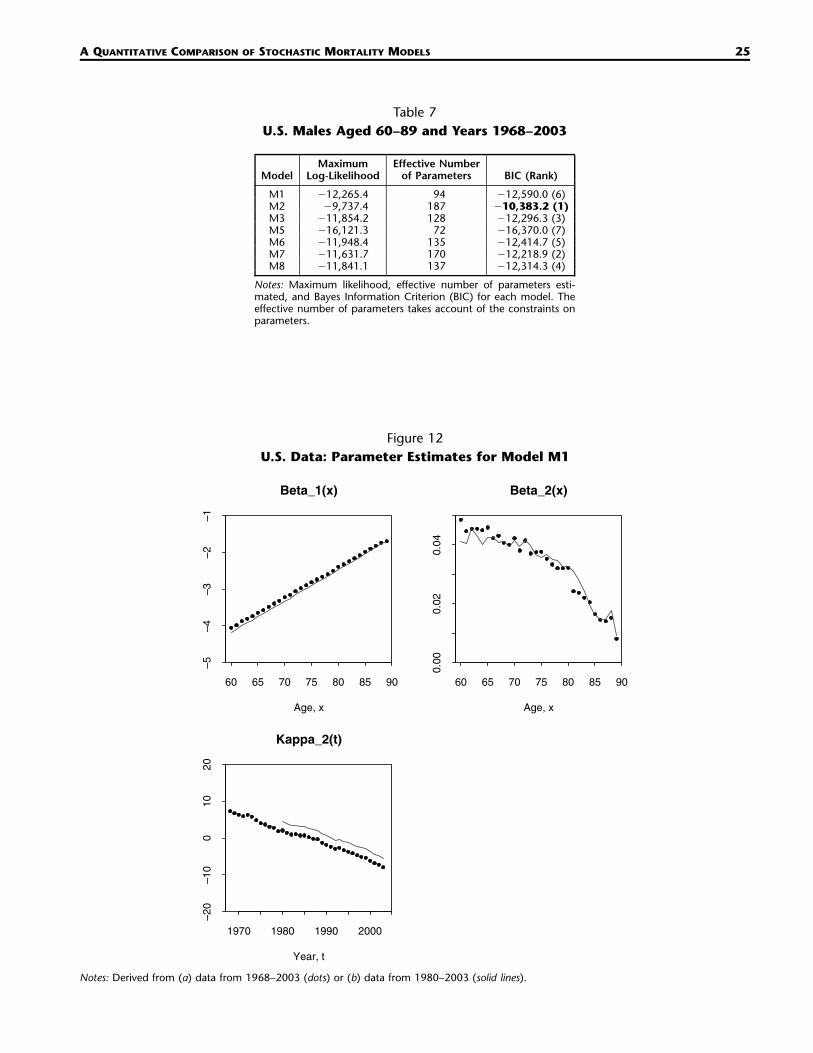
covering the period 1968–2003. Maximum likelihoods are given in Table 7. Estimates of the parametersthemselves are plotted in Figures 12–18. In these plots the dots are parameter estimates based ondata from 1968 to 2003, and lines are based on data from 1980 to 2003.
7.1.1 Bayes Information CriterionThe BIC for each model is given in the final column in Table 7. In contrast with the results in Table 3for the EW (EW) data, model M2 now comes out significantly better than the other models. However,in the subsections that follow, we will discuss graphical diagnostic tests that suggest M2 might be
A QUANTITATIVE COMPARISON OF STOCHASTIC MORTALITY MODELS 25
Table 7U.S. Males Aged 60–89 and Years 1968–2003
ModelMaximum
Log-LikelihoodEffective Number
of Parameters BIC (Rank)
M1 �12,265.4 94 �12,590.0 (6)M2 �9,737.4 187 �10,383.2 (1)M3 �11,854.2 128 �12,296.3 (3)M5 �16,121.3 72 �16,370.0 (7)M6 �11,948.4 135 �12,414.7 (5)M7 �11,631.7 170 �12,218.9 (2)M8 �11,841.1 137 �12,314.3 (4)
Notes: Maximum likelihood, effective number of parameters esti-mated, and Bayes Information Criterion (BIC) for each model. Theeffective number of parameters takes account of the constraints onparameters.
Figure 12U.S. Data: Parameter Estimates for Model M1
60 65 70 75 80 85 90
–5–4
–3–2
–1
Beta_1(x)
Age, x
60 65 70 75 80 85 90
0.00
0.02
0.04
Beta_2(x)
Age, x
1970 1980 1990 2000
–20
–10
010
20
Kappa_2(t)
Year, t
Notes: Derived from (a) data from 1968–2003 (dots) or (b) data from 1980–2003 (solid lines).
26 NORTH AMERICAN ACTUARIAL JOURNAL, VOLUME 13, NUMBER 1
Figure 13U.S. Data: Parameter Estimates for Model M2
60 65 70 75 80 85 90
–4.5
–4.0
–3.5
–3.0
–2.5
–2.0
–1.5
Beta_1(x)
Age, x
60 65 70 75 80 85 90
0.00
0.02
0.04
0.06
0.08
Beta_2(x)
Age, x
1970 1980 1990 2000
–4–2
02
4
Kappa_2(t)
Year, t
60 65 70 75 80 85 90
0.02
00.
025
0.03
00.
035
0.04
00.
045
Beta_3(x)
Age, x
1880 1900 1920 1940
–20
–10
010
20
Gamma_3(t)
Year, t
Notes: Derived from (a) Data from 1968–2003 (dots), (b) Data from 1980–2003 (solid lines). Crosses in the bottom left plot correspond toexcluded cohorts.

A QUANTITATIVE COMPARISON OF STOCHASTIC MORTALITY MODELS 27
Figure 14U.S. Data: Parameter Estimates for Model M3
60 65 70 75 80 85 90
–5–4
–3–2
–1
Beta_1(x)
Age, x
1970 1980 1990 2000
–10
–50
510
Kappa_2(t)
Year, t
1880 1900 1920 1940
–6–4
–20
2
Gamma_3(t)
Year, t
Notes: Derived from (a) Data from 1968–2003 (dots), (b) Data from 1980–2003 (solid lines). Crosses in the bottom left plot correspond toexcluded cohorts.
Figure 15U.S. Data: Parameter Estimates for Model M5
1970 1980 1990 2000
–3.2
–3.0
–2.8
–2.6
–2.4
Kappa_1(t)
Year, t
1970 1980 1990 2000
0.07
00.
080
0.09
00.
100
Kappa_2(t)
Year, t
Notes: Derived from (a) Data from 1968–2003 (dots), (b) Data from 1980–2003 (solid lines).

28 NORTH AMERICAN ACTUARIAL JOURNAL, VOLUME 13, NUMBER 1
Figure 16U.S. Data: Parameter Estimates for Model M6
1970 1980 1990 2000
–3.2
–3.0
–2.8
–2.6
–2.4
Kappa_1(t)
Year, t
1970 1980 1990 2000
0.07
50.
085
0.09
50.
105
Kappa_2(t)
Year, t
1880 1900 1920 1940
–0.0
50.
000.
050.
10
Gamma_3(t)
Year, t
Notes: Derived from (a) Data from 1968–2003 (dots), (b) Data from 1980–2003 (solid lines). Crosses in the bottom left plot correspond toexcluded cohorts.
overfitting the data (especially when it is suspected—as discussed in Section 2.2—that the exposuresdata contain significant errors), and lead us to doubt its robustness.
7.1.2 Standardized ResidualsThe variances of the standardized residuals for the U.S. data are very much higher than for EW (Table4). Using 1968–2003 data, the variance is around 7.5 for model M2 and 11.5 for models M7 and M8.Using data from 1980 to 2003, these fall to about 3.3 and 7.5, respectively. As discussed before, if thedata were wholly reliable, the Poisson assumption the right one, and the model the correct one, thenthis variance should be around 1. The high values we see here, therefore, lend weight to our earlierremarks concerning inaccuracies in the exposures data.
The plots of standardized residuals (not presented here) exhibit some degree of clustering. Out ofthese M2 looks the most random, but comparison of this with its EW counterpart suggests that M2fits the U.S. data less well in terms of the i.i.d. assumption.

A QUANTITATIVE COMPARISON OF STOCHASTIC MORTALITY MODELS 29
Figure 17U.S. Data: Parameter Estimates for Model M7
1970 1980 1990 2000
–3.2
–3.0
–2.8
–2.6
–2.4
Kappa_1(t)
Year, t
1970 1980 1990 2000
0.07
50.
085
0.09
5
Kappa_2(t)
Year, t
1970 1980 1990 2000–2 e
-04
1 e
-04
4 e
-04
Kappa_3(t)
Year, t
1880 1900 1920 1940
–0.0
50.
000.
050.
10
Gamma_4(t)
Year, t
Notes: Derived from (a) Data from 1968–2003 (dots), (b) Data from 1980–2003 (solid lines). Crosses in the bottom right plot correspond toexcluded cohorts.
7.1.3 Comparison of Nested ModelsWe carried out likelihood ratio tests on models that are nested, as an alternative to model selectionusing the BIC.
Test results for all seven nested pairs are presented in Table 8. These results support our earlierconclusions based on the BIC: namely, that the more complex models succeed in fitting the data betterthan the simpler models.
One can compare Tables 5 and 8 to investigate the relative importance of specific model features.For example, compare M6 with M7. With the U.S. data, the test statistic is larger than the EW teststatistic with fewer degrees of freedom, and this indicates that the quadratic age effect is more prom-inent in the U.S. data.
7.2 Parameter Estimates and Their RobustnessParameter estimates for the seven models are plotted in Figures 12–18. For those that incorporate acohort effect, this effect is quite prominent. However, the form of the effect does seem to vary from
30 NORTH AMERICAN ACTUARIAL JOURNAL, VOLUME 13, NUMBER 1
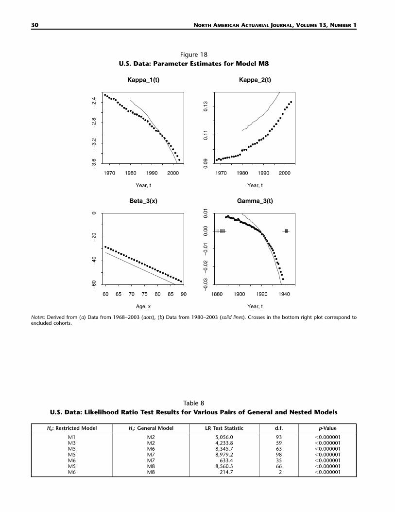
Figure 18U.S. Data: Parameter Estimates for Model M8
1970 1980 1990 2000
–3.6
–3.2
–2.8
–2.4
Kappa_1(t)
Year, t
1970 1980 1990 2000
0.09
0.11
0.13
Kappa_2(t)
Year, t
60 65 70 75 80 85 90
–60
–40
–20
0
Beta_3(x)
Age, x
1880 1900 1920 1940
–0.0
3–0
.02
–0.0
10.
000.
01Gamma_3(t)
Year, t
Notes: Derived from (a) Data from 1968–2003 (dots), (b) Data from 1980–2003 (solid lines). Crosses in the bottom right plot correspond toexcluded cohorts.
Table 8U.S. Data: Likelihood Ratio Test Results for Various Pairs of General and Nested Models
H0: Restricted Model H1: General Model LR Test Statistic d.f. p-Value
M1M3M5M5M6M5M6
M2M2M6M7M7M8M8
5,056.04,233.88,345.78,979.2
633.48,560.5
214.7
9359639835662
�0.000001�0.000001�0.000001�0.000001�0.000001�0.000001�0.000001

A QUANTITATIVE COMPARISON OF STOCHASTIC MORTALITY MODELS 31
one model to another (e.g., M3 versus M7). We will focus our remaining remarks on models M2, M7,and M8.
Comparing Figure 13 with its EW counterpart, Figure 4, the patterns for M2 are quite different. Thestrong, almost linear trend in is rather indicative of a steady period effect that is independent of(3)�c
the period effect.20 Consequently, although M2 scores the highest BIC, Figure 13 suggests that a(2)�t
variation on M2 with an additional period factor might be better.A further concern about the suitability of M2 arises when we look at estimates for and These(2) (3)� � .x x
display a much higher degree of randomness than we saw in the EW data. As we have discussed inSection 4.9, we would expect to see smoothness in each of the age effects: it is difficult to think ofany biological or environmental factors that would result in this level of randomness in and(2) (3)� � .x x
Rather, the randomness suggests M2 might be overfitting the U.S. data.21
Now compare Figure 17 (model M7) with its EW counterpart Figure 8. The pattern of developmentof the various parameters in M7 is fairly consistent between the two countries. The main qualitativedifference that we can identify under model M7 is that has a less well-defined pattern in the U.S.(4)�c
results, and a greater degree of randomness. This suggests that cohort-related trends in mortality areless important in the United States than in EW. What remains of a cohort effect in the U.S. data mightbe the result of overfitting or perhaps due to genuine environmental factors that affect each cohort intheir year of birth and that vary randomly from year to year (e.g., influenza epidemics).
For model M8 (Fig. 18), the trend in is similar to the M2 cohort effect (Fig. 13). As with M2,(3)�t�x
therefore, it suggests that the model might be improved by the inclusion of an additional period effect.
7.2.1 RobustnessFigures 12–18 also include parameter estimates for each model based on data from 1980 to 2004(solid lines in the plots). If we compare these with the original parameter estimates based on datafrom 1968 to 2003 (dots), we can make similar observations about each model as in the case of EWdata. The simpler models, M1, M3, and M5, tend to show greater robustness.22 M7 again seems to bethe most robust out of M2, M7, and M8, while M2 again has problems, leading us to question itsreliability as a means of projecting mortality rates.
7.3 Model Forecasting Properties
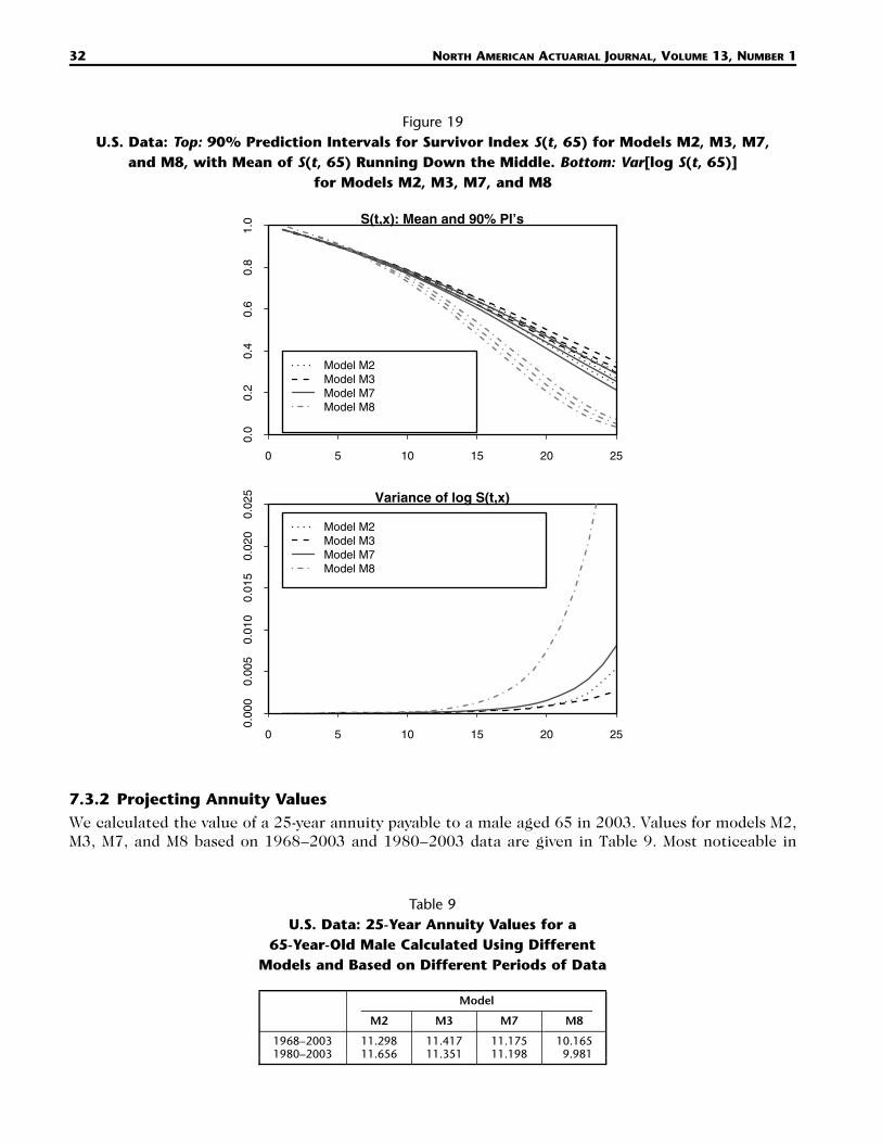
7.3.1 Survivor Index ProjectionsIt is interesting and informative to consider the differences between projections using the four modelswith the top four BIC rankings (in order, M2, M7, M3, and M8). In Figure 19 (top) we have plottedthe mean and 90% prediction intervals for the survivor index S(t, 65): that is, the proportion out ofthose alive and aged 65 in 2003 surviving to year 2003 � t.23 Models M2, M3, and M7 produce relativelysimilar projections, although the prediction interval for M3 is narrower—a feature that is more obviousif we look at the variance of log S(t, 65) (Fig. 19, bottom).
M8 stands out as being substantially different. The steepening of around 1920 in combination(3)�c
with the negative fitted values for (Fig. 18) implies that cohorts born after 1920 have increasingly(3)�x
poor mortality relative to the improving trend. This form of cohort effect also appears in model(1)�t
M6, but not in any of the other models. As a consequence, M8 relative to M2, M3, and M7 has sub-stantially lower survival rates in the 2003 age-65 cohort.
20 That is, and are not identical.(2) (3)� �x x21 A possible future refinement of M2, therefore, might be to replace the fully nonparametric with a smooth function of x by applying the(2)�x
method of P-splines.22 Much of the shifts we see in models M1 and M3 could be eliminated by adjusting the constraints.23 See the appendix for further details.
32 NORTH AMERICAN ACTUARIAL JOURNAL, VOLUME 13, NUMBER 1
Figure 19U.S. Data: Top: 90% Prediction Intervals for Survivor Index S(t, 65) for Models M2, M3, M7,
and M8, with Mean of S(t, 65) Running Down the Middle. Bottom: Var[log S(t, 65)]for Models M2, M3, M7, and M8
0 5 10 15 20 25
0.0
0.2
0.4
0.6
0.8
1.0
Model M2Model M3Model M7Model M8
S(t,x): Mean and 90% PI’s
0 5 10 15 20 25
0.00
00.
005
0.01
00.
015
0.02
00.
025
Model M2Model M3Model M7Model M8
Variance of log S(t,x)
7.3.2 Projecting Annuity ValuesWe calculated the value of a 25-year annuity payable to a male aged 65 in 2003. Values for models M2,M3, M7, and M8 based on 1968–2003 and 1980–2003 data are given in Table 9. Most noticeable in
Table 9U.S. Data: 25-Year Annuity Values for a
65-Year-Old Male Calculated Using DifferentModels and Based on Different Periods of Data
Model
M2 M3 M7 M8
1968–20031980–2003
11.29811.656
11.41711.351
11.17511.198
10.1659.981

A QUANTITATIVE COMPARISON OF STOCHASTIC MORTALITY MODELS 33
this table are the relatively low values for M8, which reflects the unusual cohort effect discussed in theprevious subsection. We can also see that the relative lack of robustness in parameter estimates underM2 and M8 means that values under these two models are more sensitive to changes in the period ofdata used than M3 and M7.
8. CONCLUSIONS
We have attempted to explain mortality improvements for males aged 60–89 in England and Wales(EW) and in the United States using a number of stochastic mortality models that decompose mortalityimprovements into one or more age-, period-, and cohort-related effects. No single model stands outas being best under all the selection criteria considered. However, different models have differentstrengths. For example, the Lee-Carter class of models allows for greater flexibility in the age effects,
while one-dimensional P-splines can be exploited to smooth age effects if the roughness of the(i)� ,x
is seen as a drawback. For their part the CBD-Perks models impose smoothness in the age effects(i)�x
as an assumption, but allow for richer period effects than the Lee-Carter class. We therefore need tobalance up the strengths and weaknesses of each model to form a conclusion, and to some extent itis up to potential users of the models to decide the weights they place on the different criteria.
If the reader looks only at the BIC ranking criterion, then model M8 for the EW data and model M2for the U.S. data dominate. However, if the reader takes into account the robustness of the parameterestimates, then model M7 is preferred for both datasets. This model fits both datasets well, and thestability of the parameter estimates over time enables one to place some degree of trust in its projec-tions of mortality rates. The lack of robustness in the other models means that we cannot wholly relyon projections produced by them.
Model M7 shows that mortality rates in both England and Wales and the United States have thefollowing features in common (see Figs. 8 and 17):
• Mortality rates have been improving over time at all ages: the ‘‘level’’ period term has been(1)(� )t
declining over time, so that the upward-sloping plot of the logit of mortality rates against age hasbeen shifting downwards over time.
• These improvements have been greater at lower ages than at higher ages: the ‘‘slope’’ period termhas been increasing over time, so that the plot of the logit of mortality rates against age has(2)(� )t
been steepening as it shifts downwards over time. This phenomenon has been noted by the studiessurveyed in Wong-Fupuy and Haberman (2004, Sections 5.2 and 5.3), for example.
• The changes over time in and have been approximately linear, and such linear improvements(1) (2)� �t t
have also been noted in previous studies (e.g., Wong-Fupuy and Haberman 2004, Section 5.1).• Mortality rates plotted on a logistic scale against age have a slight curvature over the 60–89 age
range that can be modeled using a quadratic function of age. The inclusion of a component thatcombined a quadratic age effect with a stochastic period effect was found to be statisticallysignificant.
• There is a significant cohort effect in mortality improvements, although this is more prominent(4)(� )c
and systematic in the EW than the U.S. data.
To a large extent, these commonalities are also reflected in the other models considered.A good stochastic mortality model must take these features into account when forecasting mortality
improvements and prediction intervals around these forecasts. This is important for quantifying lon-gevity risk, for providing benchmarks for longevity-linked financial instruments (Blake and Burrows2001; Blake, Cairns, and Dowd 2006; Blake et al. 2006; Dowd et al. 2006; Dawson et al. 2007), forpricing such instruments (Cairns, Blake, and Dowd 2006a,b), and for using these instruments forhedging (Dahl and Møller 2006; Dahl, Melchior, and Møller 2008).
As noted above, our analysis has focused on males aged 60–89 in England and Wales and the UnitedStates over the last 44 years. It is important to note that if the same models are applied to different

34 NORTH AMERICAN ACTUARIAL JOURNAL, VOLUME 13, NUMBER 1
countries, to females rather than males, to a different age range, or to a different range of years, thenthe conclusions about which model is most suitable might be different.
In terms of using the models for forecasting, we have limited ourselves in this study to two briefillustrations, one looking at the survivor index and the other at annuity prices. In companion studies(Dowd et al. 2008a,b; Cairns et al. 2008), we investigate the goodness-of-fit, backtesting, and fore-casting properties of the models in more detail.
APPENDIX
SIMULATION MODEL
For projection of the survivor index, S(t, x), we need to take the fitted parameter values illustrated inFigures 3–9 and 12–18 and use these to develop a stochastic projection model.
For example, for model M5 we use the method described in Cairns, Blake, and Dowd (2006b) (CBD):thus we fitted a two-dimensional random-walk model to using the the final 21 years of data(1) (2)(� , � )t t
(i.e., 20 observations of the change in The form of in this paper is different from the(1) (2) (2)(� , � ). �t t x
original CBD paper, so parameter estimates are different.In the main body of this paper, we report on simulation results for M2, M5, M7, and M8. For M2,
M7, and M8, the age effects are fixed. For each of M2, M7, and M8, we adopt the same principles(i)�x
for simulation of the period and cohort effects. For model M7, for example, we take the following(i) (i)� �t c
approach for EW data from 1961 to 2004:
• Fit the and to the full set of data from age 60 to 89.(i) (i) (i)� , � , �x t c
• Then take and for years 1984–2004 inclusive, and fit a three-dimensional random walk(1) (2) (3)� , � , �t t t
with drift.• For the cohorts aged 65, 70, and 75 in 2004, we already have an estimate of the cohort effect,
and so no model is required for these values.(4) (4) (4)� , � , � ,1939 1934 1929
• For the cohort aged 60 in 2004 (i.e., the 1944 birth cohort), we need to project the estimated (4)�c
series. Our results clearly indicate that a random walk model is inappropriate, but the developmentof a more suitable model for is beyond the scope of this study. If we wish to model the survivor(4)�c
index, S(t, 60), for this cohort (which in turn will allow us to calculate annuity values), we need asingle value (simulated or otherwise) for only, and not for any other years. Based on the his-(4)�1944
torical development of we try out two values for (one high and one low) to cover what we(4) (4)� , �c 1944
feel is the likely range of values that might be taken by (4)� .1944
Once we have our simulation model for S(t, x) we can calculate 4% term annuity values according tothe formula
90�x�1.04ta (2004) � e E[S(t, x)].�x
t�1
In this expression, the upper age limit of age 90 is imposed to avoid the requirement to extrapolatebeyond the range of ages used in the model fitting process, thereby allowing us to focus on projectionof the period and cohort effects.
REFERENCES
ANDERSON, R. N. 1999. Method for Constructing Complete Annual U.S. Life Tables. Vital and Health Statistics 2(129), National Centerfor Health Statistics.
BLAKE, D., AND W. BURROWS. 2001. Survivor Bonds: Helping to Hedge Mortality Risk. Journal of Risk and Insurance 68: 339–48.BLAKE, D., A. J. G. CAIRNS, AND K. DOWD. 2006. Living with Mortality: Longevity Bonds and Other Mortality-Linked Securities. British
Actuarial Journal 12: 153–97.BLAKE, D., A. J. G. CAIRNS, K. DOWD, AND R. MACMINN. 2006. Longevity Bonds: Financial Engineering, Valuation and Hedging. Journal
of Risk and Insurance 73: 647–72.

A QUANTITATIVE COMPARISON OF STOCHASTIC MORTALITY MODELS 35
BROUHNS, N., M. DENUIT, AND J. K. VERMUNT. 2002. A Poisson Log-Bilinear Regression Approach to the Construction of Projected LifeTables. Insurance: Mathematics and Economics 31: 373–93.
CAIRNS, A. J. G. 2000. A Discussion of Parameter and Model Uncertainty in Insurance. Insurance: Mathematics and Economics 27:313–30.
CAIRNS, A. J. G., D. BLAKE, AND K. DOWD. 2006a. Pricing Death: Frameworks for the Valuation and Securitization of Mortality Risk.ASTIN Bulletin 36: 79–120.
———. 2006b. A Two-Factor Model for Stochastic Mortality with Parameter Uncertainty: Theory and Calibration. Journal of Risk andInsurance 73: 687–718.
———. 2008. Measurement, Modelling and Management of Mortality Risk: A Review. Scandinavian Actuarial Journal, (2–3): 79–113.CAIRNS, A. J. G., D. BLAKE, K. DOWD, G. D. COUGHLAN, D. EPSTEIN, AND M. KHALAF-ALLAH. 2008. Mortality Density Forecasts: An Analysis
of Six Stochastic Mortality Models. Working paper, Heriot-Watt University, and Pensions Institute Discussion Paper PI-0801.CONTINUOUS MORTALITY INVESTIGATION BUREAU (CMI). 2005. Projecting Future Mortality: Towards a Proposal for a Stochastic Meth-
odology. Working paper 15.———. 2006. Stochastic Projection Methodologies: Further Progress and P-Spline Model Features, Example Results and Implications.
Working paper 20.———. 2007. Stochastic Projection Methodologies: Lee-Carter Model Features, Example Results and Implications. Working paper 25.CURRIE, I. D. 2006. Smoothing and Forecasting Mortality Rates with P-Splines. Paper given at the Institute of Actuaries, June 2006.
http://www.ma.hw.ac.uk/�iain/research/talks.html.CURRIE, I. D., M. DURBAN, AND P. H. C. EILERS. 2004. Smoothing and Forecasting Mortality Rates. Statistical Modelling 4: 279–98.CZADO, C., A. DELWARDE, AND M. DENUIT. 2005. Bayesian Poisson Log-Linear Mortality Projections. Insurance: Mathematics and Eco-
nomics 36: 260–84.DAHL, M., M. MELCHIOR, AND T. MøLLER. 2008. On Systematic Mortality Risk and Risk Minimisation with Survivor Swaps. Scandinavian
Actuarial Journal (2–3): 114–46.DAHL, M., AND T. MøLLER. 2006. Valuation and Hedging of Life Insurance Risks with Systematic Mortality Risk. Insurance: Mathematics
and Economics 39: 193–217.DAWSON, P., D. BLAKE, A. J. G. CAIRNS, AND K. DOWD. 2007. Completing the Survivor Derivatives Market. Pensions Institute Discussion
Paper PI-0712.DOWD, K., D. BLAKE, A. J. G. CAIRNS, G. D. COUGHLAN, D. EPSTEIN, AND M. KHALAF-ALLAH. 2008a. Evaluating the Goodness of Fit of
Stochastic Mortality Models. Pensions Institute Discussion Paper PI-0802.———. 2008b. Backtesting Stochastic Mortality Models: An Ex-Post Evaluation of Multi-Period-Ahead Density Forecasts. Pensions
Institute Discussion Paper PI-0803.DOWD, K., D. BLAKE, A. J. G. CAIRNS, AND P. DAWSON. 2006. Survivor Swaps. Journal of Risk and Insurance 73: 1–17.DOWD, K., A. J. G. CAIRNS, AND D. BLAKE. 2006. Mortality-Dependent Financial Risk Measures. Insurance: Mathematics and Economics
38: 427–40.HAYASHI, F. 2000. Econometrics. Princeton: Princeton University Press.JACOBSEN, R., N. KEIDING, AND E. LYNGE. 2002. Long-Term Mortality Trends behind Low Life Expectancy of Danish Women. Journal
of Epidemiology and Community Health 56: 205–8.KOISSI, M. C., A. F. SHAPIRO, AND G. HOGNAS. 2006. Evaluating and Extending the Lee-Carter Model for Mortality Forecasting: Bootstrap
Confidence Intervals. Insurance: Mathematics and Economics 38: 1–20.LEE, R. D., AND L. R. CARTER. 1992. Modeling and Forecasting U.S. Mortality. Journal of the American Statistical Association 87: 659–
75.OSMOND, C. 1985. Using Age, Period and Cohort Models to Estimate Future Mortality Rates. International Journal of Epidemiology
14: 124–29.PERKS, W. 1932. On Some Experiments in the Graduation of Mortality Statistics. Journal of the Institute of Actuaries 63: 12–57.RENSHAW, A. E., AND S. HABERMAN. 2003. Lee-Carter Mortality Forecasting with Age-Specific Enhancement. Insurance: Mathematics
and Economics 33: 255–72.———. 2006. A Cohort-Based Extension to the Lee-Carter Model for Mortality Reduction Factors. Insurance: Mathematics and Eco-
nomics 38: 556–70.RICHARDS, S. J., J. G. KIRKBY, AND I. D. CURRIE. 2006. The Importance of Year of Birth in Two-Dimensional Mortality Data. British
Actuarial Journal 12: 5–38.WILLETS, R. C. 1999. Mortality in the Next Millennium. Paper presented to the Staple Inn Actuarial Society.———. 2004. The Cohort Effect: Insights and Explanations. British Actuarial Journal 10: 833–77.WONG-FUPUY, C., AND S. HABERMAN. 2004. Projecting Mortality Trends: Recent Developments in the United Kingdom and the United
States. North American Actuarial Journal 8(1): 56–83.
Discussions on this paper can be submitted until July 1, 2009. The authors reserve the right to reply to anydiscussion. Please see the Submission Guidelines for Authors on the inside back cover for instructions on thesubmission of discussions.