Remote Sens. 2019, 11, x; doi:

Article

An Improved Hatch Filter Algorithm towards Sub-

Meter Positioning Using only Android Raw GNSS

Measurements without External Augmentation

Corrections

Jianghui Geng, Enming Jiang, Guangcai Li, Shaoming Xin * and Na Wei

1 GNSS Research Center, Wuhan University, Wuhan 430079, China; jgeng@whu.edu.cn (J.G.);

guangcai.li@whu.edu.cn (G.L.); jem@whu.edu.cn (E.J.); nwei@whu.edu.cn (N.W.)

* Correspondence: jsx_miracle@whu.edu.cn (S.X.); Tel.:+86-155-2712-1159

Abstract: In May 2016, the availability of GNSS raw measurements on smart devices was announced

by Google with the release of Android 7. It means that developers can access carrier-phase and

pseudorange measurements and decode navigation messages for the first time from mass-market

Android-devices. In this paper, an improved Hatch filter algorithm, i.e., Three-Thresholds and

Single-Difference Hatch filter (TT-SD Hatch filter), is proposed for sub-meter single point

positioning with raw GNSS measurements on Android devices without any augmentation

correction input, where the carrier-phase smoothed pseudorange window width adaptively varies

according to the three-threshold detection for ionospheric cumulative errors, cycle slips and outliers.

In the mean time, it can also eliminate the inconsistency of receiver clock bias between pseudorange

and carrier-phase by inter-satellite difference. To eliminate the effects of frequent smoothing

window resets, we combine TT-SD Hatch filter and Kalman filter for both time update and

measurement update. The feasibility of the improved TT-SD Hatch filter method is then verified

using static and kinematic experiments with a Nexus 9 Android tablet. The result of the static

experiment demonstrates that the position RMS of TT-SD Hatch filter is about 0.6 and 0.8 m in the

horizontal and vertical components, respectively. It is about 2 and 1.6 m less than the GNSS chipset

solutions, and about 10 and 10 m less than the classical Hatch filter solution, respectively. Moreover,

the TT-SD Hatch filter can accurately detect the cycle slips and outliers, and reset the smoothed

window in time. It thus avoids the smoothing failure of Hatch filter when a large cycle-slip or an

outlier occurs in the observations. Meanwhile, with the aid of the Kalman filter, TT-SD Hatch filter

can keep continuously positioning at the sub-meter level. The result of the kinematic experiment

demonstrates that the TT-SD Hatch filter solution can converge after a few minutes, and the 2D

error is about 0.9 m, which is about 64%, 89%, and 92% smaller than that of the chipset solution, the

traditional Hatch filter solution and standard single point solution, respectively. Finally, the TT-SD

Hatch filter solution can recover a continuous driving track in this kinematic test.

Keywords: Raw GNSS Measurement; Android devices; Hatch filter; Phase-smoothed pseudorange

1. Introduction

As a general impression, we can get a rough position through the consumer-grade chipset in

smartphones based on Global Navigation Satellite System (GNSS) observations. The accuracy of the

GPS modules embedded in smartphones is typically 3–5 m under good multi-path conditions;

otherwise, it can be above 10 m [1]. Meanwhile, previous works have been focusing on different

characteristics of GNSS reception and smartphone GNSS performance under different conditions

[2,3]. However, as the positioning accuracy of GNSS chipsets improves, the existing devices are likely

to be updated and location-based services will become further diversified. Appreciably, achieving

Remote Sens. 2019, 11, x FOR PEER REVIEW 2 of 21

positioning and navigation with sub-meter-level accuracy on smart devices with a consumer-grade

chipset is an important application for the future development of mass-market GNSS [4]. Therefore,

sub-meter-level positioning is urgently required to meet the demands of the high-precision Location

Based Services (LBS) [5]. With the release of Android 7, Google announced that the raw GNSS

measurements in Android smart devices can be exported and used through the API (Application

Programming Interface) at the application level. Thus, it is possible for us to make use of the GNSS

raw measurements from the low-cost Android smart terminal for high-precision navigation and

positioning. On the other hand, from 2017 to 2020, GNSS receivers in the global market will grow

from 5.8 billion to 8.0 billion, in which the smart portable devices that people use almost every day

account for almost 80% of the total amount [6]. It means that research on high-precision positioning

and navigation of smart devices has great prospects in the market. The official Android

documentation illustrates most Android 7.0 or higher smart devices manufactured in 2016 or later

can provide raw GNSS data [7].

These GNSS raw measurements from Android devices mainly include the pseudorange, carrier-

phase, and Doppler measurements. The pseudorange measurements from the Android-devices

combined with broadcast ephemeris can be processed using standard point positioning to provide

the user with the meter-level position [8]. Warnant has proposed that carrier phase-based static

differential positioning using GPS and Galileo (L1/E1+L5/E5a) on a very short baseline provides cm-

level precision in the horizontal component and decimeter-level in the vertical component by using

a XiaoMi 8 (XiaoMi, China) smartphone [9]. K. Asari used a smartphone-grade antenna and receiver

combined with SSR corrections which achieved positioning at the sub-meter level [10]. Meanwhile,

D. Calle proposed the MagicPPP method combined with IMU (Inertial Measurement Unit) data from

Android-devices, which can reach decimeter-level accuracy [11]. D. Laurichesse developed an

application named PPP Wizlite, which can provide positions with a sub-meter level accuracy in static

mode and with meter-level accuracy in dynamic mode with online precise satellite corrections [12].

However, a high-precision position obtained by the PPP method needs an online statement and more

electric power. Therefore, the point that combines carrier-phase observations with pseudorange

observations to attain a high-precision position without any additional corrections for an Android

device is worthy of research.

Previous research has found that smoothing the pseudorange measurements with Doppler

measurements and carrier-phase measurements can reduce the pseudorange noise and improve the

positioning accuracy for the traditional geodetic GNSS receivers [13]. Hatch filter algorithm is a

classical phase-smoothed pseudorange algorithm in the existing smoothing filters [14,15]. For the

classical Hatch filter algorithm, the selection of the smoothing windows is a difficult and significant

step. If the smoothing window is too long, the ionospheric cumulative errors are too large and the

filtering will diverge [16]. On the contrary, if the smoothing window is too short, the smoothing effect

is not obvious. Park applied an optimal constant to the classical Hatch filter to reduce the ionospheric

cumulative errors [17]. Euiho Kim proposed an adaptive carrier smoothing method to weaken the

active ionospheric error and severe multipath error [18]. However, there is a big amount of cycle slips

in the carrier-phase measurements for Android devices, which is a non-negligible problem for the

pseudorange smoothing algorithm as it needs to calculate the phase difference between adjacent

epochs. Cycle slips may lead to a devastating influence on the result with the smoothing algorithm

[19]. Liu proposed an improved Hatch filter algorithm for the duty-cycle disuse of smartphones [20].

H. K. Lee proposed an improved position-domain Hatch filter, which is advantageous in real-time

kinematic positioning and cycle slip detection based on dual frequency observations [21]. Besides,

previous research has proposed that for Android smart devices, the clock bias in the carrier phase

observation is not the same as the clock bias in the pseudorange observation [22]. Therefore, we

construct single-difference observations between satellites to weaken this inequality. In addition,

Helena has implemented a fusion filter to combine carrier phase, pseudorange and Doppler to obtain

the smoothing position in kinematic tests [23]. In dynamic mode, we use the Kalman filter combined

with phase-smoothed pseudorange and Doppler observations for velocity-aided positioning. Based

on the above analysis, we will propose an enhanced algorithm based on the Hatch filter and the

Remote Sens. 2019, 11, x FOR PEER REVIEW 3 of 21

Kalman filter algorithms, which use variable smoothing window widths dealing with ionospheric

delay cumulative errors, cycle slips and outliers in the GNSS observations of Android-devices. Our

study is based on the Nexus 9 (Google, America) tablet because it can provide continuous carrier

phase observation without duty cycle.

In the following, firstly, the release of GNSS observations after Android N system and the

respective data collection applications are briefly reviewed. Secondly, a classical phase-smoothed

pseudorange using Hatch filter algorithm and three threshold detections for ionosphere cumulative

errors, cycle slips and gross errors of observations from Android devices are discussed, following

which the three thresholds-single difference Hatch filter algorithm, i.e., TT-SD Hatch filter algorithm,

is proposed. Subsequently, the specific suppression effects of the Three-Thresholds and Single-

Difference (TT-SD) Hatch filter algorithm on the ionospheric delay cumulative errors, cycle slips, and

outliers, are verified by experiments. In the next section, the quality analyses of pseudorange and

carrier-phase observations are discussed and the experiment design, results, and experimental

analysis are outlined. Finally, the discussion and conclusions are presented.

2. Methods

2.1. Acquisition of GNSS Measurements

Although we can acquire raw GNSS information, we cannot obtain the pseudorange and carrier-

phase measurements directly from Android devices through the API at the application level. We

should first carry on a series of transformations on the parameters provided with the corresponding

APIs to obtain the pseudorange and carrier-phase measurements. The reception time of the GNSS

signal in the GPS time system Rxt is computed as:

Rx TimeNanos FullBiasNanos BiasNano nst s

(1)

where TimeNanos denotes the GNSS receiver internal hardware clock value in nanoseconds;

FullBiasNanos denotes the difference between the hardware clock inside the GPS receiver and the true

GPS time since 6 January 1980 (GPS time start reference); and BiasNanos denotes the clock sub-

nanosecond bias [24]. After computing the reception time in the GPS time system, the pseudorange

P can be deduced using Equation (2):

( )*Rx TxP t t c (2)

where c is the speed of light and Txt is the transmitted time of the GPS signal in the GPS time

system calculated by the getReceivedSvTimeNanos function of Android API 24 [24].

Meanwhile, we can derive carrier-phase measurements from the AccumulatedDeltaRangeMeters

observations calculated by the getAccumulatedDeltaRangeMeters function of Android API 24. The

mathematical relationship between the AccumulatedDeltaRangeMeters parameter and carrier-phase

measurement is expressed by the following equation:

*( - )AccumulatedDeltaRangeMeters k carrier phase (3)

where k is the wavelength of carrier-phase data. The Doppler shift that results from satellite

movement can be derived from the getPseudorangeRateMetersPerSecond function of Android API 24 in

m/s [24].

We used the data collection applications GnssLogger (V 2.0.0.1 Release) to collect the raw GNSS

data, [25] whilst the collected raw GNSS data are processed and converted into the RINEX 3.0 format

by our own software.

2.2. Phase-Smoothed Pseudorange

Phase-smoothed pseudorange can decrease the noise of pseudorange. Among all the smoothing

techniques, the Hatch filter is a type of recursive filter that uses the current measurement and

previous estimate without any dynamic model or additional sensors, and it can be implemented for

Remote Sens. 2019, 11, x FOR PEER REVIEW 4 of 21

real-time operation in a low-cost single-frequency GNSS receiver [16]. The equation of the Hatch filter

is as follows:

1 1( ) ( ) ( ( 1) ( ) ( 1))

(1) (1)

nP n P n P n n n

n n

P P

(4)

where ( )n and ( 1)n denote the carrier-phase observation at thn and ( 1)thn epoch,

respectively; ( )P n and ( 1)P n denote the smoothed pseudorange at the thn and ( 1)thn epoch,

respectively; and ( )P n denotes the pseudorange measurement at the thn epoch. Through Equation

(4) we can find that as the measured values increase, the pseudorange will be smoothed and

measurement noise will be decreased. As the single difference between epochs is used, ambiguity

has been subtracted when no cycle slips occur.

Previous research has proposed that for Android devices, the receiver clock bias in the carrier

phase raw observation may not be the same as the clock bias in the pseudorange [22]. To avoid the

possible influence of this inequality, we use the single difference between satellites. Therefore, we

establish the smoothed pesudorange observations with a single difference between satellites based

on the Hatch filter smoothing algorithm, as described in Equation (5):

, , , , ,

,

,

, ,

1 1(n) ( ) ( ( 1) ( ) ( 1))

(1) (1)

s A s A s A s A s A

s As A

s As A

s A s A

nP P n P n n n

n n

P P P

P P

(5)

where A and s represent the reference satellite and the non-reference satellite, respectively; A

P

and sP denote the raw pseudorange observations of satellites A and s , respectively, while

A

and s

denote the raw carrier-phase observation of satellites A and s ; and ,s AP ,

,s AP and ,s A denote the single difference raw pseudorange, smoothed pseudorange and carrier-phase

observation between the reference satellite A and the non-reference satellite s , respectively.

Besides, in our algorithm, we choose the satellite with the highest elevation as the reference satellite.

2.3. Threshold Detection for Ionosphere Delay Cumulative Error

The observation equation for single-difference pseudorange and carrier-phase between satellites is:

,

,

, , , , ,

, , , , , ,

+

+

s A

s A

s A s A s A s A s A

P

s A s A s A s A s A s A

P cdT I T

cdT I T N

(6)

In the above equations, ,s A is the single difference carrier-phase observation;

,s A is the

single difference distance between the satellite and receiver; ,s AdT is the single difference satellite

clock bias between the reference satellite A and the non-reference satellite s ; ,s AI and ,s AT

represent the single difference propagation delay of the ionosphere and troposphere; and ,s AP

and

,s A

are the sum of all remaining errors of single difference pseudorange and carrier phase

respectively. Based on Equation (6), we use the epoch-differenced method between thn and ( 1)thn

epoch and the transformed observation equation can be described in Equation (7):

Remote Sens. 2019, 11, x FOR PEER REVIEW 5 of 21

,

,

, , , , , ,

, , , , , ,

( ) ( 1) ( 1) ( 1)+ ( 1) ( 1)+

( ) ( 1) ( 1) ( 1) ( 1) ( 1)+

s A

s A

s A s A s A s A s A s A

P

s A s A s A s A s A s A

P n P n n n cdT n n I n n T n n

n n n n cdT n n I n n T n n

， ， ， ，

， ， ， ， (7)

Although the Hatch filter performs excellently in reducing noise and is easy to implement under

normal conditions, the ionosphere-related term should not be ignored and should be compensated

in the phase-smoothed pseudorange as described:

, , , , ,( ) ( 1)= ( ) ( 1) 2 ( 1)s A s A s A s A s An n P n P n I n n ， (8)

Equations (5) and (8) show that as the observation time increases, the ionosphere delay errors

are gradually accumulated in Hatch filter processing. In order to reduce the influence of the

ionosphere delay cumulative errors, it needs to reset the window and re-smooth observations when

this error exceeds the pseudorange measurement range. We use the difference between the smoothed

pseudorange and the raw pseudorange to detect whether the ionosphere delay cumulative errors

reach the threshold and reset the filter window:

, ,

1(n) (n)s A s AP P (9)

where 1 denotes the detection threshold and 1=3 2 P is set according to the 3σ-Rule and

variance-covariance propagation law, where P is the standard deviation of pseudorange

measurement error.

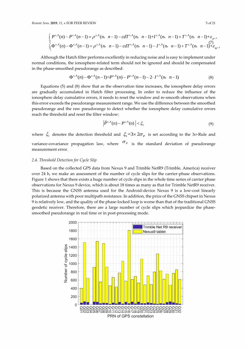
2.4. Threshold Detection for Cycle Slip

Based on the collected GPS data from Nexus 9 and Trimble NetR9 (Trimble, America) receiver

over 24 h, we make an assessment of the number of cycle slips for the carrier-phase observations.

Figure 1 shows that there exists a huge number of cycle slips in the whole time series of carrier phase

observations for Nexus 9 device, which is about 18 times as many as that for Trimble NetR9 receiver.

This is because the GNSS antenna used for the Android-device Nexus 9 is a low-cost linearly

polarized antenna with poor multipath resistance. In addition, the price of the GNSS chipset in Nexus

9 is relatively low, and the quality of the phase-locked loop is worse than that of the traditional GNSS

geodetic receiver. Therefore, there are a large number of cycle slips which jeopardize the phase-

smoothed pseudorange in real time or in post-processing mode.

Remote Sens. 2019, 11, x FOR PEER REVIEW 6 of 21

Figure 1. Cycle slips of carrier-phase observations over 24 h.

In order to mitigate the influence of cycle slips, we perform cycle slip detection by the

relationship between Doppler and phase change rate. When a cycle slip occurs, the phase-smoothed

pseudorange window is reset to re-smooth observations. The cycle slip detection and threshold are

designed as follows: [26]

2

( ) ( 1)( ) ( 1)

2

D n D nn n t

(10)

where ( )D n and ( 1)D n represent the Doppler observations at thn and ( 1)thn epoch,

respectively; ( ) ( 1)n n represents the phase change rate by single difference between the

thn and ( 1)thn epoch; t denotes time interval; and 2 denotes the cycle slip threshold, which

is valued as one cycle when t is 1s.

2.5. Threshold Detection for Outliers

As we know, if the outliers (such as observation biases) in the GNSS observations cannot be

accurately detected and properly removed, the pseudorange smoothing may be seriously affected or

even fail. We use the difference between the pseudorange rate and the phase rate to detect outliers.

The difference between ( ( ) ( -1))P n P n and ( ) ( 1)n n is 2 ( 1)I n n ， , and the epoch-

difference ionospheric delay ( 1)I n n， is much smaller. When an outlier occurs in the

pseudorange or phase, a large number is introduced. Therefore, we set the following threshold

detection:

3( ( ) ( -1)) ( ) ( 1)P n P n n n (11)

where 3 denotes the detection threshold and 3=3 2 P is set according to the 3σ-Rule

and variance-covariance propagation law, where P is the standard deviation of pseudorange

measurement error.

2.6. Three-Thresholds and Single-Difference Hatch Filter Algorithm

Based on the above analysis, we eliminate the receiver clock inconsistency between the

pseudorange and the phase by the single difference between the satellites. Meanwhile, we introduce

these three threshold detections into the Hatch filter to adaptively adjust the smoothing window

length, in order to weaken the influence of the ionosphere cumulative errors, cycle slips, and gross

errors. Therefore, we call this method: three thresholds–single difference Hatch filter algorithm (TT-

SD Hatch-Filter). Figure 2 presents the whole process of the algorithm.

Remote Sens. 2019, 11, x FOR PEER REVIEW 7 of 21

Figure 2. The architecture of TT-SD (Three-Thresholds and Single-Difference Hatch filter) Hatch filter

algorithm

In detail, the processing procedures of our TT-SD Hatch filter include:

1. Input raw GNSS (Global Navigation Satellite System) observations;

2. Form a single-difference carrier phase and pseudorange observations between the reference

satellite and non-reference satellite;

3. Phase-smoothed pseudorange by Hatch filter;

4. Three thresholds detection: While the difference between the smoothed pseudorange and true

pseudorange (t1) is less than the threshold (ξ1) for ionosphere delay cumulative errors, the

phase rate prediction residual by Doppler observations (t2) is less than the threshold (ξ2) for the

cycle slip, and the difference between the pseudorange rate and the phase rate (t3) is less than

the threshold (ξ3) for outliers; the smoothing window width accumulates and the smoothed

pseudorange observations are available for positioning. Otherwise, the smoothing window is

re-initialized.

5. If the smoothing window was initialized and the condition t3<ξ3 holds, the raw pseudorange

observations are used for positioning, or else no pseudorange observations are available for

positioning at this epoch.

6. Repeat step 1–5 above for all epochs of GNSS observations to obtain the smoothed

pseudorange observations for positioning.

2.7. Three-Thresholds and Single-Difference Hatch Filter Algorithm with Kalman Filter

In the process of obtaining a smoothed pseudorange using the TT-SD Hatch filter algorithm, if

any one of the thresholds is exceeded, the smoothing window will be reset and the continuity

between the epochs for the position parameters will be destroyed. In particular, the frequent

occurrence of cycle slips and outliers in Android devices makes this problem more serious. Therefore,

we use the Kalman filter for state update and measurement update to obtain smoothed position

results. When the user is in the kinematic mode, the Doppler observations are used to estimate the

velocity of the user, which is combined with the position of the user to construct the state vector of

the system. The position of the user is only estimated on the static mode. The recurrence model is

described as Equation (12):

Remote Sens. 2019, 11, x FOR PEER REVIEW 8 of 21

, 1 1k k k k k X φ X Q (12)

where k denotes the thk epoch; X denotes the state vector of the receiver; φ denotes the state

transition matrix between epochs; and Q denotes the processing noise vector. When applying the

kinematic mode, assuming T is the sampling interval, X , φ and Q can be described as:

0 0 0

, , , , , 0 0 0

0 0

x x

y y

z z

x v a

y v a

z v a

2

a

TI T

r 2

φX 0 I T r v a QV

0 0 I qa

(13)

where r , V and a denote the vector of position, velocity, and accelerometer of the receiver,

respectively; and aq denotes the processing noise of the accelerometer, which usually denotes a

diagonal matrix. When applying the static mode, different from Equation (13), X , φ and Q can

be described as:

, , ,

x

y

z

rX r φ I r Q q (14)

The state vector only includes the position r of the receiver. rq denotes the processing noise

of the position. The clock bias and the clock rate of the receiver are not included in the state vector

X , because the single difference between satellites eliminates the influence of clock bias and clock

rate; I denotes a 3×3 unit matrix. Besides, in our algorithm, we have set the initial state error

covariance matrix of position as described:

x 0 0

0 0

0 0

y

z

Var

Var

Var

rP (15)

where xVar , yVar and zVar represent the error covariance of the position of user [ ]x y z .

Meanwhile, in kinematic mode, the initial state error covariance matrix of velocity and acceleration

as described:

0 0 0 0

0 0 , 0 0

0 0 0 0

x x

y y

z z

v a

v a

v a

Var Var

Var Var

Var Var

v aP P = (16)

where xvVar ,

yvVar and zvVar represent the error covariance of the velocity of the user [ ]x y zv v v ;

xaVar , yaVar and

zaVar represent the error covariance of the acceleration of the user [ ]x y za a a .

The predicted covariance matrix can be calculated with 1| 1k k P using the following equation:

| 1 1| 1

T

k k k k k k k P φ P φ Q (17)

After computing the gain matrix kK , the matrix |k kP can be updated. kH denotes the design

matrix. kR is the covariance matrix of observation noise.

Remote Sens. 2019, 11, x FOR PEER REVIEW 9 of 21

1

| 1 | 1

| | 1

( + )

( )

T T

k k k k k k k k k

k k k k k k

K P H H P H R

P I K H P

， (18)

The smoothed inter-satellite difference pseudorange and Doppler observation equations are

described as:

,

, , , , ,c* s Ak

s A s A s A s A s A

k k PP dT I T (19)

,

, , ,* s Ak

s A s A s A

k k DD c dT (20)

where s and A denote the non-reference satellite and reference satellite, respectively; ,s A

kP

denotes the smoothed inter-satellite difference peseudorange after TT-SD Hatch filter processing at

epoch k ; ,s A

k and ,s A

k denote the inter-satellite difference range and range-rate between the

receiver and the satellites s , A ; and ,s A

kD respectively denote the wavelength of L1 signal and

inter-satellite difference Doppler observation; ,s AdT denotes the inter-satellite difference satellite

clock bias rate. In addition, ,s AI and ,s AT are corrected by the Klobuchar and Saastamoinen models,

respectively. [27,28]

For the kinematic mode, the measurement formula in our system can be described in Equation (21):

,

,

( ) ( ) ( ) ( ) ( ) ( )

, ,

( ) ( ) ( ) ( ) ( ) ( )

a A a A a A a A a A a A

k k k k k k k k k k k ks A

k

k k k k k ks A

k s A s A s A s A s A s A

k k k k k k k k k k k k

l l m m n n l l m m n n

l l m m n n l l m m n n

PZ H X ν Z H

DM M M M M M

(21)

where kZ denotes the measurement vector; kH denotes the design matrix, in which index a to

s denote non-reference satellite and A denotes reference satellite; [ ]a a a

k k kl m n , [ ]s s s

k k kl m n and

[ ]A A A

k k kl m n denote direction cosine vector between the satellite and receiver for satellites a , s and

A , respectively; kν denotes the measurement noise, which depends on the smoothing window

width and the signal to noise ratio of the observations [29]. For the static mode, different from

Equation (21), the measurement formula is described as:

,

( ) ( ) ( )

, ,

( ) ( ) ( )

a A a A a A

k k k k k k

s A

k k k k k k k

s A s A s A

k k k k k k

l l m m n n

l l m m n n

Z H X ν Z P H M M M (22)

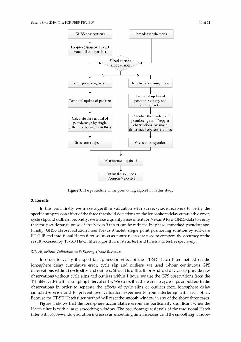
The flowchart of our positioning algorithm is shown in Figure 3. Firstly, the GNSS observations

obtained by smartphones are pre-processed by TT-SD Hatch-filter algorithm to obtain the smoothed

pseudorange. Secondly, either kinematic or static processing mode is selected by the user. Thirdly,

after processing with the Kalman filter algorithm, the estimated parameters, such as position and

velocity are generated.

Remote Sens. 2019, 11, x FOR PEER REVIEW 10 of 21

Figure 3. The procedure of the positioning algorithm in this study

3. Results

In this part, firstly we make algorithm validation with survey-grade receivers to verify the

specific suppression effect of the three threshold detections on the ionosphere delay cumulative error,

cycle slip and outliers. Secondly, we make a quality assessment for Nexus 9 Raw GNSS data to verify

that the pseudorange noise of the Nexus 9 tablet can be reduced by phase-smoothed pseudorange.

Finally, GNSS chipset solution inner Nexus 9 tablet, single point positioning solution by software

RTKLIB and traditional Hatch filter solution as comparisons are used to compare the accuracy of the

result accessed by TT-SD Hatch filter algorithm in static test and kinematic test, respectively.

3.1. Algorithm Validation with Survey-Grade Receivers

In order to verify the specific suppression effect of the TT-SD Hatch filter method on the

ionosphere delay cumulative error, cycle slip and outliers, we used 1-hour continuous GPS

observations without cycle slips and outliers. Since it is difficult for Android devices to provide raw

observations without cycle slips and outliers within 1 hour, we use the GPS observations from the

Trimble NetR9 with a sampling interval of 1 s. We stress that there are no cycle slips or outliers in the

observations in order to separate the effects of cycle slips or outliers from ionosphere delay

cumulative error and to prevent two validation experiments from interfering with each other.

Because the TT-SD Hatch filter method will reset the smooth window in any of the above three cases.

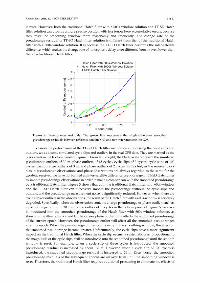
Figure 4 shows that the ionosphere accumulative errors are particularly significant when the

Hatch filter is with a large smoothing window. The pseudorange residuals of the traditional Hatch

filter with 3600s-window solution increases as smoothing time increases until the smoothing window

Remote Sens. 2019, 11, x FOR PEER REVIEW 11 of 21

is reset. However, both the traditional Hatch filter with a 600s-window solution and TT-SD Hatch

filter solution can provide a more precise position with less ionosphere accumulative errors, because

they reset the smoothing window more reasonably and frequently. The change rate of the

pseudorange residual of TT-SD Hatch filter solution is different from that of the traditional Hatch

filter with a 600s-window solution. It is because the TT-SD Hatch filter performs the inter-satellite

difference, which makes the change rate of ionospheric delay error different from or even lower than

that of a traditional Hatch filter.

Figure 4. Pseudorange residuals. The green line represents the single-difference smoothed

pseudorange residuals between reference satellite G03 and non-reference satellite G29.

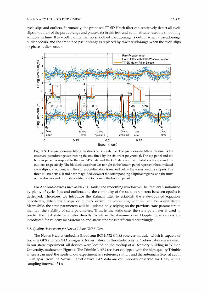
To assess the performance of the TT-SD Hatch filter method on suppressing the cycle slips and

outliers, we add some simulated cycle slips and outliers in the real GPS data. They are marked as the

black ovals in the bottom panel of Figure 5. From left to right, the black ovals represent the simulated

pseudorange outliers of 30 m, phase outliers of 15 cycles, cycle slips of 3 cycles, cycle slips of 100

cycles, pseudorange outliers of 3 m, and phase outliers of 2 cycles. In this test, as the receiver clock

bias in pseudorange observations and phase observations are always regarded as the same for the

geodetic receiver, we have not formed an inter-satellite difference pseudorange in TT-SD Hatch filter

to smooth pseudorange observations in order to make a comparison with the smoothed pseudorange

by a traditional Hatch filter. Figure 5 shows that both the traditional Hatch filter with 600s-window

and the TT-SD Hatch filter can effectively smooth the pseudorange without the cycle slips and

outliers, and the pseudorange measurement noise is significantly reduced. However, when there are

cycle slips or outliers in the observations, the result of the Hatch filter with a 600s-window is seriously

degraded. Specifically, when the observation contains a large pseudorange or phase outlier, such as

a pseudorange outlier of 30 m or phase outlier of 15 cycles in the bottom panel of Figure 5, an error

is introduced into the smoothed pseudorange of the Hatch filter with 600s-window solution, as

shown in the illustrations a and b. The carrier phase outlier only affects the smoothed pseudorange

of the current epoch. However, the pseudorange outlier will affect all the smoothed pseudoranges

after the epoch. When the pseudorange outlier occurs early in the smoothing window, the effect on

the smoothed pseudorange become greater. Unfortunately, the cycle slips have a more significant

impact on the traditional Hatch filter. When the cycle slip occurs, a systematic bias, proportional to

the magnitude of the cycle slips, will be introduced into the smoothed pseudorange until the smooth

window is reset. For example, when a cycle slip of three cycles is introduced, the smoothed

pseudorange residual is increased by about 0.6 m. However, when a cycle slip of 100 cycles is

introduced, the smoothed pseudorange residual is increased to 20 m. Even worse, the smoothed

pseudorange residuals of the subsequent epochs are all over 10 m until the smoothing window is

reset. Therefore, the traditional Hatch filter requires additional processing to eliminate the effects of

Remote Sens. 2019, 11, x FOR PEER REVIEW 12 of 21

cycle slips and outliers. Fortunately, the proposed TT-SD Hatch filter can sensitively detect all cycle

slips or outliers of the pseudorange and phase data in this test, and automatically reset the smoothing

window in time. It is worth noting that no smoothed pseudorange is output when a pseudorange

outlier occurs, and the smoothed pseudorange is replaced by raw pseudorange when the cycle slips

or phase outliers occur.

Figure 5. The pseudorange fitting residuals of G29 satellite. The pseudorange fitting residual is the

observed pseudorange subtracting the one fitted by the six-order polynomial. The top panel and the

bottom panel correspond to the raw GPS data and the GPS data with simulated cycle slips and the

outliers, respectively. The black ellipses from left to right in the bottom panel represent the simulated

cycle slips and outliers, and the corresponding data is marked below the corresponding ellipses. The

three illustrations a, b and c are magnified views of the corresponding elliptical regions, and the units

of the abscissa and ordinate are identical to those of the bottom panel.

For Android-devices such as Nexus 9 tablet, the smoothing window will be frequently initialized

by plenty of cycle slips and outliers, and the continuity of the state parameters between epochs is

destroyed. Therefore, we introduce the Kalman filter to establish the state-updated equation.

Specifically, when cycle slips or outliers occur, the smoothing window will be re-initialized.

Meanwhile, the state parameters will be updated only relying on the previous state parameters to

maintain the stability of state parameters. Thus, in the static case, the state parameter is used to

predict the next state parameter directly. While in the dynamic case, Doppler observations are

introduced for velocity measurement, and status update is performed accordingly.

3.2. Quality Assessment for Nexus 9 Raw GNSS Data

The Nexus 9 tablet embeds a Broadcom BCM4752 GNSS receiver module, which is capable of

tracking GPS and GLONASS signals. Nevertheless, in this study, only GPS observations were used.

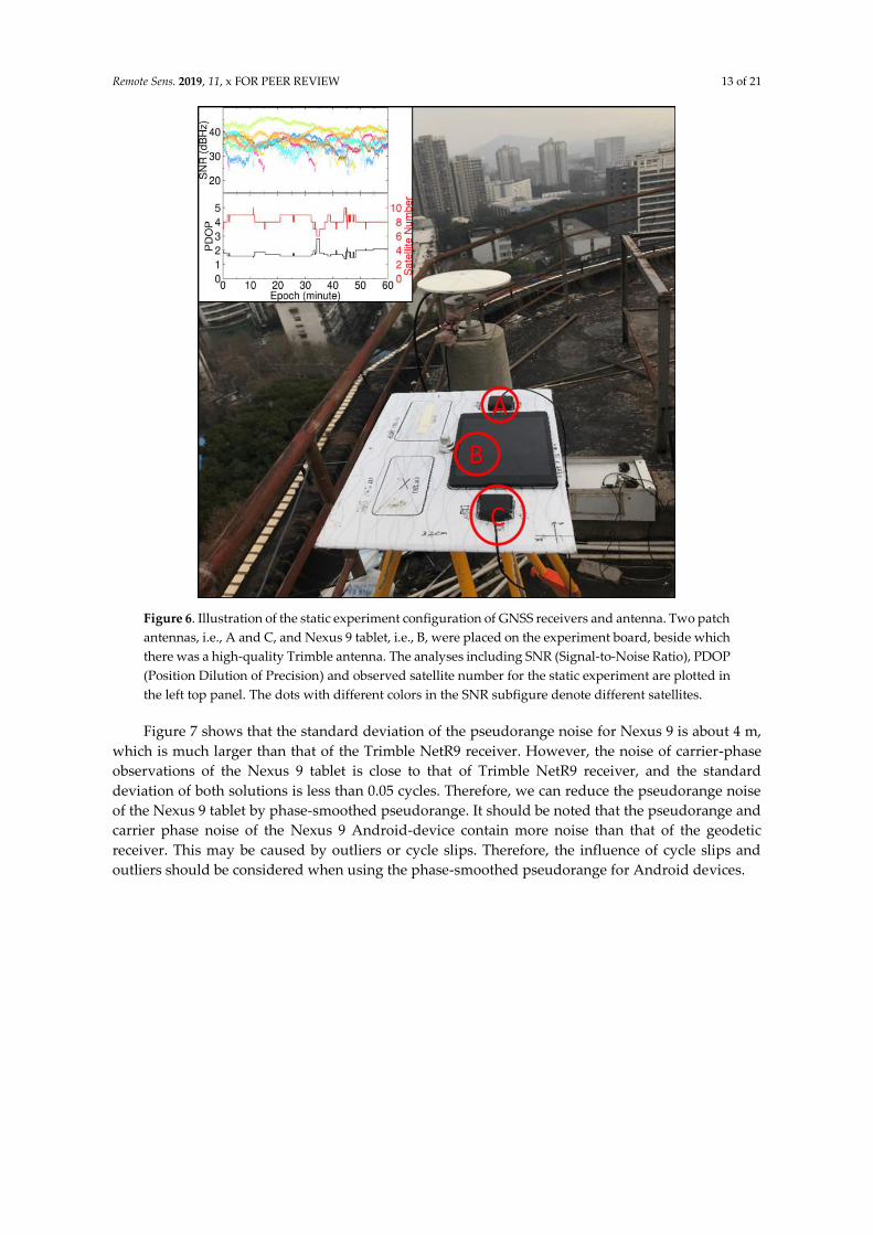
In our static experiment, all devices were located on the rooftop of a 16th-story building in Wuhan

University, as shown in Figure 6. The Trimble NetR9 receiver equipped with the high-quality Trimble

antenna can meet the needs of our experiment as a reference station, and the antenna is fixed at about

0.5 m apart from the Nexus 9 tablet device. GPS data are continuously observed for 1 day with a

sampling interval of 1 s.

Remote Sens. 2019, 11, x FOR PEER REVIEW 13 of 21

Figure 6. Illustration of the static experiment configuration of GNSS receivers and antenna. Two patch

antennas, i.e., A and C, and Nexus 9 tablet, i.e., B, were placed on the experiment board, beside which

there was a high-quality Trimble antenna. The analyses including SNR (Signal-to-Noise Ratio), PDOP

(Position Dilution of Precision) and observed satellite number for the static experiment are plotted in

the left top panel. The dots with different colors in the SNR subfigure denote different satellites.

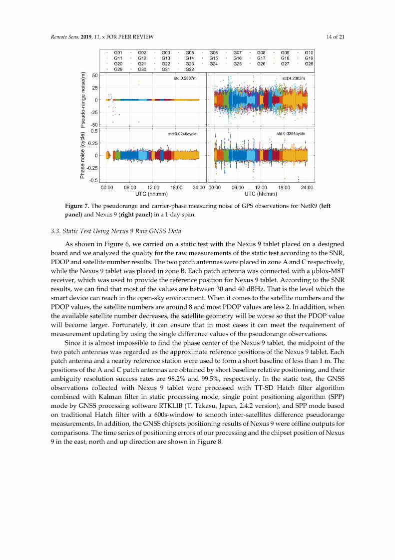
Figure 7 shows that the standard deviation of the pseudorange noise for Nexus 9 is about 4 m,

which is much larger than that of the Trimble NetR9 receiver. However, the noise of carrier-phase

observations of the Nexus 9 tablet is close to that of Trimble NetR9 receiver, and the standard

deviation of both solutions is less than 0.05 cycles. Therefore, we can reduce the pseudorange noise

of the Nexus 9 tablet by phase-smoothed pseudorange. It should be noted that the pseudorange and

carrier phase noise of the Nexus 9 Android-device contain more noise than that of the geodetic

receiver. This may be caused by outliers or cycle slips. Therefore, the influence of cycle slips and

outliers should be considered when using the phase-smoothed pseudorange for Android devices.

Remote Sens. 2019, 11, x FOR PEER REVIEW 14 of 21

Figure 7. The pseudorange and carrier-phase measuring noise of GPS observations for NetR9 (left

panel) and Nexus 9 (right panel) in a 1-day span.

3.3. Static Test Using Nexus 9 Raw GNSS Data

As shown in Figure 6, we carried on a static test with the Nexus 9 tablet placed on a designed

board and we analyzed the quality for the raw measurements of the static test according to the SNR,

PDOP and satellite number results. The two patch antennas were placed in zone A and C respectively,

while the Nexus 9 tablet was placed in zone B. Each patch antenna was connected with a μblox-M8T

receiver, which was used to provide the reference position for Nexus 9 tablet. According to the SNR

results, we can find that most of the values are between 30 and 40 dBHz. That is the level which the

smart device can reach in the open-sky environment. When it comes to the satellite numbers and the

PDOP values, the satellite numbers are around 8 and most PDOP values are less 2. In addition, when

the available satellite number decreases, the satellite geometry will be worse so that the PDOP value

will become larger. Fortunately, it can ensure that in most cases it can meet the requirement of

measurement updating by using the single difference values of the pseudorange observations.

Since it is almost impossible to find the phase center of the Nexus 9 tablet, the midpoint of the

two patch antennas was regarded as the approximate reference positions of the Nexus 9 tablet. Each

patch antenna and a nearby reference station were used to form a short baseline of less than 1 m. The

positions of the A and C patch antennas are obtained by short baseline relative positioning, and their

ambiguity resolution success rates are 98.2% and 99.5%, respectively. In the static test, the GNSS

observations collected with Nexus 9 tablet were processed with TT-SD Hatch filter algorithm

combined with Kalman filter in static processing mode, single point positioning algorithm (SPP)

mode by GNSS processing software RTKLIB (T. Takasu, Japan, 2.4.2 version), and SPP mode based

on traditional Hatch filter with a 600s-window to smooth inter-satellites difference pseudorange

measurements. In addition, the GNSS chipsets positioning results of Nexus 9 were offline outputs for

comparisons. The time series of positioning errors of our processing and the chipset position of Nexus

9 in the east, north and up direction are shown in Figure 8.

Remote Sens. 2019, 11, x FOR PEER REVIEW 15 of 21

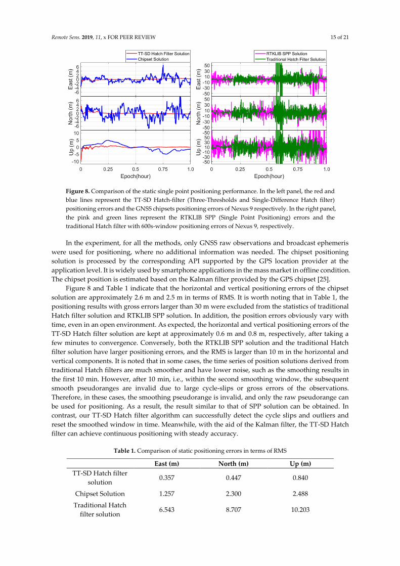
Figure 8. Comparison of the static single point positioning performance. In the left panel, the red and

blue lines represent the TT-SD Hatch-filter (Three-Thresholds and Single-Difference Hatch filter)

positioning errors and the GNSS chipsets positioning errors of Nexus 9 respectively. In the right panel,

the pink and green lines represent the RTKLIB SPP (Single Point Positioning) errors and the

traditional Hatch filter with 600s-window positioning errors of Nexus 9, respectively.

In the experiment, for all the methods, only GNSS raw observations and broadcast ephemeris

were used for positioning, where no additional information was needed. The chipset positioning

solution is processed by the corresponding API supported by the GPS location provider at the

application level. It is widely used by smartphone applications in the mass market in offline condition.

The chipset position is estimated based on the Kalman filter provided by the GPS chipset [25].

Figure 8 and Table 1 indicate that the horizontal and vertical positioning errors of the chipset

solution are approximately 2.6 m and 2.5 m in terms of RMS. It is worth noting that in Table 1, the

positioning results with gross errors larger than 30 m were excluded from the statistics of traditional

Hatch filter solution and RTKLIB SPP solution. In addition, the position errors obviously vary with

time, even in an open environment. As expected, the horizontal and vertical positioning errors of the

TT-SD Hatch filter solution are kept at approximately 0.6 m and 0.8 m, respectively, after taking a

few minutes to convergence. Conversely, both the RTKLIB SPP solution and the traditional Hatch

filter solution have larger positioning errors, and the RMS is larger than 10 m in the horizontal and

vertical components. It is noted that in some cases, the time series of position solutions derived from

traditional Hatch filters are much smoother and have lower noise, such as the smoothing results in

the first 10 min. However, after 10 min, i.e., within the second smoothing window, the subsequent

smooth pseudoranges are invalid due to large cycle-slips or gross errors of the observations.

Therefore, in these cases, the smoothing pseudorange is invalid, and only the raw pseudorange can

be used for positioning. As a result, the result similar to that of SPP solution can be obtained. In

contrast, our TT-SD Hatch filter algorithm can successfully detect the cycle slips and outliers and

reset the smoothed window in time. Meanwhile, with the aid of the Kalman filter, the TT-SD Hatch

filter can achieve continuous positioning with steady accuracy.

Table 1. Comparison of static positioning errors in terms of RMS

East (m) North (m) Up (m)

TT-SD Hatch filter

solution 0.357 0.447 0.840

Chipset Solution 1.257 2.300 2.488

Traditional Hatch

filter solution 6.543 8.707 10.203

Remote Sens. 2019, 11, x FOR PEER REVIEW 16 of 21

RTKLIB SPP

solution 7.803 10.065 12.667

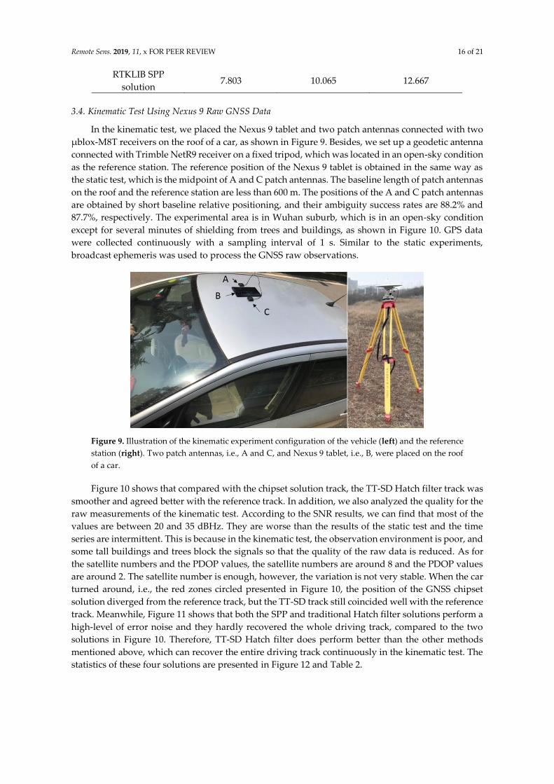
3.4. Kinematic Test Using Nexus 9 Raw GNSS Data

In the kinematic test, we placed the Nexus 9 tablet and two patch antennas connected with two

μblox-M8T receivers on the roof of a car, as shown in Figure 9. Besides, we set up a geodetic antenna

connected with Trimble NetR9 receiver on a fixed tripod, which was located in an open-sky condition

as the reference station. The reference position of the Nexus 9 tablet is obtained in the same way as

the static test, which is the midpoint of A and C patch antennas. The baseline length of patch antennas

on the roof and the reference station are less than 600 m. The positions of the A and C patch antennas

are obtained by short baseline relative positioning, and their ambiguity success rates are 88.2% and

87.7%, respectively. The experimental area is in Wuhan suburb, which is in an open-sky condition

except for several minutes of shielding from trees and buildings, as shown in Figure 10. GPS data

were collected continuously with a sampling interval of 1 s. Similar to the static experiments,

broadcast ephemeris was used to process the GNSS raw observations.

Figure 9. Illustration of the kinematic experiment configuration of the vehicle (left) and the reference

station (right). Two patch antennas, i.e., A and C, and Nexus 9 tablet, i.e., B, were placed on the roof

of a car.

Figure 10 shows that compared with the chipset solution track, the TT-SD Hatch filter track was

smoother and agreed better with the reference track. In addition, we also analyzed the quality for the

raw measurements of the kinematic test. According to the SNR results, we can find that most of the

values are between 20 and 35 dBHz. They are worse than the results of the static test and the time

series are intermittent. This is because in the kinematic test, the observation environment is poor, and

some tall buildings and trees block the signals so that the quality of the raw data is reduced. As for

the satellite numbers and the PDOP values, the satellite numbers are around 8 and the PDOP values

are around 2. The satellite number is enough, however, the variation is not very stable. When the car

turned around, i.e., the red zones circled presented in Figure 10, the position of the GNSS chipset

solution diverged from the reference track, but the TT-SD track still coincided well with the reference

track. Meanwhile, Figure 11 shows that both the SPP and traditional Hatch filter solutions perform a

high-level of error noise and they hardly recovered the whole driving track, compared to the two

solutions in Figure 10. Therefore, TT-SD Hatch filter does perform better than the other methods

mentioned above, which can recover the entire driving track continuously in the kinematic test. The

statistics of these four solutions are presented in Figure 12 and Table 2.

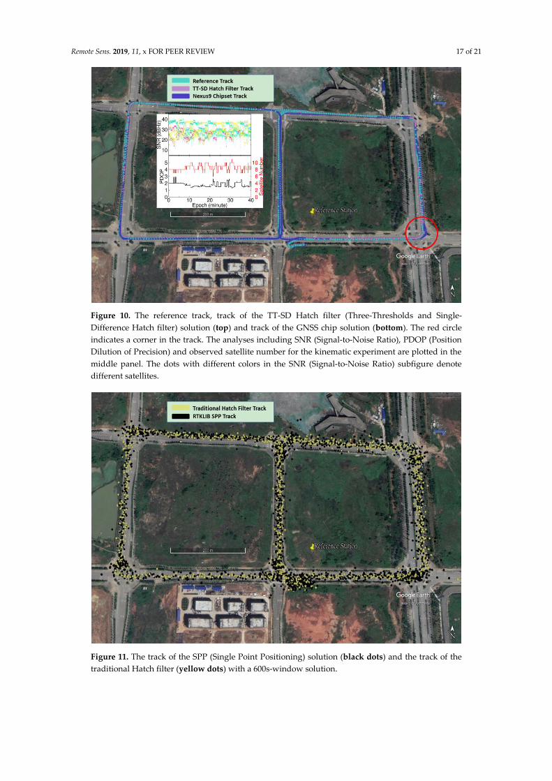
Remote Sens. 2019, 11, x FOR PEER REVIEW 17 of 21

Figure 10. The reference track, track of the TT-SD Hatch filter (Three-Thresholds and Single-

Difference Hatch filter) solution (top) and track of the GNSS chip solution (bottom). The red circle

indicates a corner in the track. The analyses including SNR (Signal-to-Noise Ratio), PDOP (Position

Dilution of Precision) and observed satellite number for the kinematic experiment are plotted in the

middle panel. The dots with different colors in the SNR (Signal-to-Noise Ratio) subfigure denote

different satellites.

Figure 11. The track of the SPP (Single Point Positioning) solution (black dots) and the track of the

traditional Hatch filter (yellow dots) with a 600s-window solution.

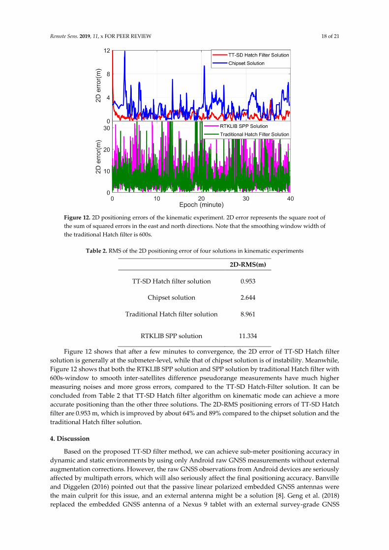
Remote Sens. 2019, 11, x FOR PEER REVIEW 18 of 21

Figure 12. 2D positioning errors of the kinematic experiment. 2D error represents the square root of

the sum of squared errors in the east and north directions. Note that the smoothing window width of

the traditional Hatch filter is 600s.

Table 2. RMS of the 2D positioning error of four solutions in kinematic experiments

2D-RMS(m)

TT-SD Hatch filter solution 0.953

Chipset solution 2.644

Traditional Hatch filter solution 8.961

RTKLIB SPP solution 11.334

Figure 12 shows that after a few minutes to convergence, the 2D error of TT-SD Hatch filter

solution is generally at the submeter-level, while that of chipset solution is of instability. Meanwhile,

Figure 12 shows that both the RTKLIB SPP solution and SPP solution by traditional Hatch filter with

600s-window to smooth inter-satellites difference pseudorange measurements have much higher

measuring noises and more gross errors, compared to the TT-SD Hatch-Filter solution. It can be

concluded from Table 2 that TT-SD Hatch filter algorithm on kinematic mode can achieve a more

accurate positioning than the other three solutions. The 2D-RMS positioning errors of TT-SD Hatch

filter are 0.953 m, which is improved by about 64% and 89% compared to the chipset solution and the

traditional Hatch filter solution.

4. Discussion

Based on the proposed TT-SD filter method, we can achieve sub-meter positioning accuracy in

dynamic and static environments by using only Android raw GNSS measurements without external

augmentation corrections. However, the raw GNSS observations from Android devices are seriously

affected by multipath errors, which will also seriously affect the final positioning accuracy. Banville

and Diggelen (2016) pointed out that the passive linear polarized embedded GNSS antennas were

the main culprit for this issue, and an external antenna might be a solution [8]. Geng et al. (2018)

replaced the embedded GNSS antenna of a Nexus 9 tablet with an external survey-grade GNSS

Remote Sens. 2019, 11, x FOR PEER REVIEW 19 of 21

antenna [30]. The strength of the GNSS signal obtained by them was consistent with that of the

survey-grade receivers; and the multipath errors, cycle slips and outliers in the raw GNSS

observations were rare. As a result, the influence of frequent re-initialization of the TT-SD smoothing

window caused by a large number of cycle slips and outliers will be reduced, and more accurate

positioning results can be obtained for Android devices using our TT-SD filter algorithm.

In addition, in this paper, the TT-SD filter algorithm is designed based on single-frequency GPS

data of Android devices, because single-frequency GPS data are mostly provided by mainstream

Android devices. On 31 May 2018, XiaoMi 8, the world’s first dual-frequency GNSS smartphone, was

launched. It is equipped with a Broadcom BCM47755 chipset, which can provide dual-frequency

(L1/E1+L5/E5) raw GNSS observations [31,32]. Thanks to the dual-frequency observation data, we

can obtain the ionosphere-free combined observations, which will further improve the phase-

smoothing-pseudorange performance of the TT-SD algorithm. The expansion of multi constellation

is also an opportunity for Android devices to provide better GNSS positioning quality. For example,

the above-mentioned Xiaomi 8 can support the acquisition of raw observations of GPS, GLONASS,

Galileo, BeiDou and QZSS. When cycle slips or outliers occur in individual observations, the TT-SD

filter with multi-GNSS can still provide robust filtering results because of the introduction of

redundant observations without outliers. Therefore, in GNSS-adverse environments, such as urban

canyons, where signals are disturbed, multi-GNSS will provide better positioning services for

Android devices in terms of positioning availability and accuracy.

5. Conclusions

We analyzed the traditional phase-smoothed pseudorange method and its shortcomings

towards GNSS observations on Android devices. Subsequently, we introduced three thresholds

detection into the Hatch filter to adaptively adjust the smoothing window, for mitigating the impacts

of the ionosphere cumulative errors, cycle slips, and gross errors. Meanwhile, we eliminated the

receiver clock inconsistency between the pseudorange and the phase by the single difference between

the satellites. An improved Hatch filter algorithm, i.e., the TT-SD Hatch filter algorithm has been

proposed using only raw Android GNSS data without any external augmentation corrections. The

ionosphere delay cumulative errors, cycle slips and outliers suppressed by the TT-SD Hatch filter

algorithm were verified by experiments. To eliminate the effects of frequent smoothing window

resets, we combined TT-SD Hatch filter and Kalman filter for status update and measurement update

to achieve the smoothing positions. Finally, the feasibility of the method is verified by static and

kinematic experiments using raw GNSS measurements from a Nexus 9 Android tablet, and the

following conclusions are obtained.

1. The static experiment shows that the horizontal and vertical position errors of TT-SD Hatch

filter solution are about 0.6 and 0.8 m in terms of RMS, respectively, after taking a few minutes

to convergence. Conversely, the horizontal and vertical positioning errors of chipset solution

are approximately 2.6 m and 2.5 m and vary with time. Both the SPP solution and the

traditional Hatch filter solution have the position RMS exceed 10 m in horizontal and vertical

components. Moreover, the smoothing effect of the traditional Hatch filter will fail when a

large number of cycle-slips or gross errors in the observations appear. In contrast, the TT-SD

Hatch filter can accurately detect the cycle slips and gross errors and reset the smoothed

window in time, thus avoiding this problem. Meanwhile, with the aid of the Kalman filter, the

TT-SD Hatch filter can achieve continuous positioning with steady accuracy.

2. The kinematic experiment shows that the TT-SD Hatch filter solution can converge after a few

minutes, and the 2D error is about 0.9 m, which is about 64%, 89% and 92% lower than that of

the chip solution, the traditional Hatch filter solution and SPP solution, respectively.

Meanwhile, the TT-SD Hatch filter solution can recover a continuous driving track but the

solutions based on the other methods do not work. Moreover, traditional Hatch filter solution

Remote Sens. 2019, 11, x FOR PEER REVIEW 20 of 21

and SPP solution present higher-level measuring noise. However, we should note that the

vehicle-borne experiment was carried out in an open and semi-open sky-view condition which

cannot represent any GNSS-difficult environments. It is expected that our TT-SD Hatch filter

solution will be degraded in such sorts of situations, not to mention the chipset solutions and

traditional Hatch filter solutions.

Funding: This work is funded by the National Key R&D Program of China (2018YFC1504002).

Acknowledgments: We’d like to appreciate Google for their open source application named GnssLogger.

Conflicts of Interest: The authors declare no conflict of interest.

References

1. Yoon, D.; Kee, C.; Seo, J.; Park, B. Position Accuracy Improvement by Implementing the DGNSS-CP

Algorithm in Smartphones. Sensors 2016, 16, 910, doi:10.3390/s16060910.

2. Gao, H.; Groves, P.D. Environmental Context Detection for Adaptive Navigation using GNSS

Measurements from a Smartphone. J. Inst. Navig. 2018, 65, 99–116.

3. Specht, C.; Dąbrowski, P.S.; Pawelski, J.; Specht, M.; Szot, T. Comparative Analysis of Positioning Accuracy

of GNSS Receivers of Samsung Galaxy Smartphones in Marine Dynamic Measurements. Adv. Space Res.

2019, 63, 3018–3028.

4. Wang, L.; Li, Z.; Zhao, J.; Zhou, K.; Wang, Z.; Yuan, H. Smart Device-Supported BDS/GNSS Real-Time

Kinematic Positioning for Sub-Meter-Level Accuracy in Urban Location-Based Services. Sensors 2016, 16,

2201.

5. Wang, L.; Li, Z.; Yuan, H.; Zhou, K. Validation and analysis of the performance of dual-frequency single-

epoch BDS/GPS/GLONASS relative positioning. Chin. Sci. Bull. 2015, 60, 857–868. (In Chinese)

6. Warnant, R.; Warnant, Q. Raw GNSS Measurements under Android: Data Quality Analysis. Available

online: http://hdl.handle.net/2268/225378 (accessed on 30 May 2018).

7. The official Android documentation that lists partial Android devices whose raw GNSS measurements are

available online : https://developer.android.com/guide/topics/sensors/gnss

8. Banville, S.; Diggeleen, F.V. Precise positioning using raw GPS measurements from Android smartphones.

GPS World 2016, 27, 43–48.

9. Warnant, R.; Van De Vyvere, L.; Warnant, Q. Positioning with Single and Dual Frequency Smartphones

Running Android 7 or Later, In Proceedings of the ION GNSS+ 2018, Miami, FL, USA 24–28 September

2018; pp. 284–303.

10. Asari, K.; Saito, M.; Amitani, H. SSR Assist for Smartphones with PPP-RTK Processing. In Proceedings of

the ION GNSS+ 2017, Session A1: Applications of Raw GNSS Measurements from Smartphones, Portland,

OR, USA, 25–29 September 2017; pp. 130–138, doi:10.33012/2017.15147.

11. Calle, D.; Carbonell, E.; Navarro, P.; Rodríguez, I.; Roldán, P.; Tobías, G. Trends, Innovations and

Enhancements for Low-Cost PPP. In Proceedings of the ION GNSS+ 2017, Session A1: Applications of Raw

GNSS Measurements from Smartphones, Portland, OR, USA, 25–29 September 2017; pp. 139–170,

doi:10.33012/2017.15148.

12. Denis, L.; Cedric, R.; Francois-Xavier, M.; Matthieu, P. Smartphone Applications for Precise Point

Positioning. In Proceedings of the ION GNSS+ 2017, Session A1: Applications of Raw GNSS Measurements

from Smartphones, Portland, OR, USA, 25–29 September 2017; pp. 171–187, doi:10.33012/2017.15149.

13. Li, L.; Zhong, J.; Zhao, M. Doppler-Aided GNSS Position Estimation With Weighted Least Squares. IEEE

Trans. Veh. Technol. 2011, 60, 3615–3624.

14. Le, A.Q.; Teunissen, P.J.G. Recursive least-squares filtering of pseudorange measurements. In Proceedings

of the European Navigation Conference 2006, Manchester, UK, 7–10 May 2006; pp. 1–11.

15. Hatch, R. The synergism of GPS code and carrier measurements. In Proceedings of the Third International

Geodetic Symposium on Satellite Doppler Positioning, Las Cruces, NM, USA, 8–12 February 1982; pp.

1213–1231.

16. Byungwoon, P.; Cheolsoon, L.; Youngsun, Y.; Euiho, K.; Changdon, K. Optimal Divergence-Free Hatch

Filter for GNSS Single-Frequency Measurement. Sensors 2017, 17, 448.

17. Park, B.; Sohn, K.; Kee, C. Optimal Hatch Filter with an Adaptive Smoothing Window Width. J. Navig. 2008,

61, 435–454.

Remote Sens. 2019, 11, x FOR PEER REVIEW 21 of 21

18. Kim, E.; Walter, T.; Powell, J.D. Adaptive carrier smoothing using code and carrier divergence. In

Proceedings of the 2007 National Technical Meeting of The Institute of Navigation, San Diego, CA, USA,

22–24 January 2007; pp. 141–152.

19. Lei, D.; Lu, W.; Cui, X.; Yu, D. Carrier-Aided Smoothing for Real-Time Beidou Positioning. In Proceedings

of the 2012 International Conference on Information Technology and Software Engineering. Lecture Notes in

Electrical Engineering; Springer: Berlin/Heidelberg, Germany, 2013; Volume 211, pp. 29–35.

20. Liu, Q.; Ying, R.; Wang, Y.; Qian, J.; Liu, P. Pseudorange Double Difference Algorithm Based on Duty-

cycled Carrier Phase Smoothing on Low-Power Smart Devices. In Proceedings of the CSNC 2018: China

Satellite Navigation Conference (CSNC) 2018 Proceedings; Springer: Singapore, 2018; pp. 415–430.

21. Lee, H.K.; Rizos, C. Position-domain Hatch Filter for kinematic differential GPS/GNSS. IEEE Trans. Aerosp.

Electron. Syst. 2008, 44, 30–40, doi:10.1109/TAES.2008.4516987.

22. Shin, D.; Lim, C.; Park, B.; Yun, Y.; Kim, E.; Kee, C. Single-frequency Divergence-free Hatch Filter for the

Android N GNSS Raw Measurements. In Proceedings of the ION GNSS+ 2017, Session A1: Applications of

Raw GNSS Measurements from Smartphones, Portland, OR, USA, 25–29 September 2017; pp. 188–225.

23. Leppäkoski, H.; Syrjärinne, J.; Takala, J. Complementary Kalman Filter for Smoothing GPS Position with

GPS Velocity. In Proceedings of the 16th International Technical Meeting of the Satellite Division of The

Institute of Navigation (ION GPS/GNSS 2003), Portland, OR, USA, 9–21 September 2003; pp. 1201–1210.

24. The GSA GNSS Raw Measurements Task Force. Using Gnss Raw Measurements On Android Devices. Publ.

Off. Eur. Union; European GNSS Agency, 2017; P20–P24, doi:10.2878/449581.

25. Official Android application for users to logging raw GNSS measurements and chipset solutions online:

https://github.com/google/gps-measurement-tools/releases

26. Cannon, M.E.; Schwarz, K.P.; Wei, M.; Delikaraoglou, D. A consistency test of airborne GPS using multiple

monitor stations. Bull. Géodésique 1992, 66, 2–11.

27. Klobuchar, J.A. Ionospheric Time-Delay Algorithm for Single-Frequency GPS Users. IEEE Trans. Aerosp.

Electron. Syst. 1987, AES-23, 325–331.

28. Saastamoninen, J. Atmospheric Correction for the Troposphere and the Stratosphere in Radio Ranging

Satellites. Use Artif. Satell. Geod. 1972, 15, 247–251.

29. Zhang, X.; Tao, X.; Zhu, F.; Shi, X.; Wang, F. Quality assessment of GNSS observations from an Android N

smartphone and positioning performance analysis using time-differenced filtering approach. GPS Solut.

2018, 22, 70.

30. Geng, J.; Li, G.; Zeng, R.; Wen, Q.; Jiang, E. A Comprehensive Assessment of Raw Multi-GNSS

Measurements from Mainstream Portable Smart Devices. In Proceedings of the ION GNSS+ 2018, Institute

of Navigation, Miami, FL, USA, 24–28 September 2018; pp. 392–412.

31. Robustelli, U.; Baiocchi, V.; Pugliano, G. Assessment of Dual Frequency GNSS Observations from a Xiaomi

Mi 8 Android Smartphone and Positioning Performance Analysis. Electronics 2019, 8, 91.

32. World’s First Dual-Frequency GNSS Smartphone Hits the Market. Available online:

https://www.gsa.europa.eu/newsroom/news/world-s-first-dual-frequency-gnss-smartphone-hits-market

(accessed on 25 September 2018).

.