art%3A10.1007%2Fs11277-011-0468-3

Wireless Pers Commun (2013) 68:553–574DOI 10.1007/s11277-011-0468-3

A Comparison of Energy Detectability Modelsfor Cognitive Radios in Fading Environments

Selami Ciftci · Murat Torlak

Published online: 22 January 2012© Springer Science+Business Media, LLC. 2012

Abstract In this work, we first analyze the accuracy of different energy detector mod-els in approximating the exact solution in AWGN. These models motivate us to developapproximation analysis to address energy detection for fading channels. Our analysis devel-ops approximation that has almost the same performance as the exact solution in Rayleighchannels. Our new model is simple enough to derive the relationship between the requirednumber of samples (N ) and the signal-to-noise ratio for a single Rayleigh channel similar tothe one obtained for AWGN channels. We also define a fading margin for link budget calcu-lations that relates N in fading channels to AWGN channels. Furthermore, we analyze theimpact of multiple antennas for cognitive radios considering two receiver diversity schemesand quantify the improvement in performance regarding this margin. All the analytical resultsderived in this paper are verified by simulations. Finally, we have implemented and verifiedenergy detection models in our multiple antenna wireless testbed.

Keywords Cognitive radios · Spectrum sensing · Energy detector · Rayleigh fading ·Receiver diversity

1 Introduction

The scarcity of spectrum and its underutilization have led to the development of cognitiveradios [1] for wireless networks. Cognitive radios sense their environment and determinethe most appropriate communication parameters. The first step of this cognitive capability isto determine whether there exists a user or not at a given time interval in a specified band-width. Spectrum sensing techniques in cognitive radios can be classified as matched filterdetection, energy based detection and cyclostationary based detection [4,9]. Matched filter

S. CiftciR & D Department, Turk Telekom, AS, Ankara, Turkey

M. Torlak (B)Department of Electrical Engineering, The University of Texas at Dallas, Richardson, TX 75080, USAe-mail: [email protected]

123

554 S. Ciftci, M. Torlak

detection is a coherent detection method that maximizes SNR but, a priori knowledge of thesignal to be detected is necessary in this method. Cyclostationary based detection makes useof the periodicity of the signal’s statistical characteristics; however, it is a computationallyexpensive method. Although energy detectors suffer from noise level ambiguities and requiremore samples than matched filter detectors, their easy implementation makes it an attractivemethod in spectrum sensing.

Some of the well-known energy detector models to simplify the performance analysis areconsidered in this paper for AWGN channel analysis. For instance, Edell’s [3] and Torri-eri’s [11] models have been developed for low probability of intercept (LPI) radars. Theirperformance in approximating the exact energy detection solution is examined in [2]. Inaddition, the approximation of energy detectors for cognitive radios in [9] is considered asthe Berkeley model in this paper.

All of the aforementioned models have been used for analyzing the performance of energydetectors in AWGN channels due to the complexity of the exact solution. These models giveus the connection between the required number of samples, N , and SNR at a given prob-ability of false-alarm, Pf , and detection, Pd to have useful engineering insight into theenergy detection problem. We define the number of (real) independent samples N = 2T Wwhere T and W are the observation time interval and bandwidth of the primary user signal,respectively. We also define SNR of the primary user signal at the cognitive radio receiverlocation as SNR = Ps/σ

2n where Ps is the average primary user signal power over N sam-

ples and σ 2n is the noise variance of the real additive Gaussian noise samples. Note that

knowing this relationship provides cognitive radio energy detector to determine their sensingtime at a given bandwidth interval. In fading environments, on the other hand, deriving theclosed form solutions for Pf and Pd with and without diversity is the main focus in [6,7,13]and in [12]. Among these references, the first three obtain the closed form Pd solutions byintegrating the Pd expression in AWGN over SNR distribution of the fading environment.In [12], closed form solutions are obtained via characteristic function of the decision statisticin fading channels. The main idea in [12] is to find the distribution of the decision statistic infading channels. In addition to these, analytical solutions for dual antenna system cognitiveradios are given in [8]. However, these analytical results are not simple enough to derive theN − SNR relationship in fading channels with and without diversity as in AWGN channels.

In this paper, we first derive the probability density function (pdf) of the decision statisticwithout making any cumbersome computations as in [12]. Specifically, we propose a newmodel based on approximating this pdf using both convolution property and Central LimitTheorem (CLT). Our model yields simple N −SNR relationship that approximates the exactsolution in fading channels. Secondly, we introduce fade margin metric to quantify the effectof the fading environment on the performance of energy detectors. The square of the fademargin relates N per antenna in Rayleigh fading channels to N in AWGN to achieve the sameperformance level, Pd and Pf , at the same SNR in both environments. This margin can beregarded as a design rule that is used to simplify the performance analysis of energy detectorbased cognitive radios. Moreover, we also consider square-law combining and square-lawselection schemes in [7] with multiple antennas for cognitive radios to quantify the improve-ment in performance regarding this margin.

In Sect. 2, the exact energy detector solution and the models are introduced. A newapproach in finding the pdf of the decision statistic in fading environments and its approxi-mation are presented in Sect. 3 and in Sect. 4, respectively. In Sect. 5, we derive N −SNR forsingle antenna cognitive radios. The multiple antenna version of this N − SNR connectionconsidering two different diversity schemes is in Sect. 6. Fade margin and its approximation

123

Energy Detectability Models 555

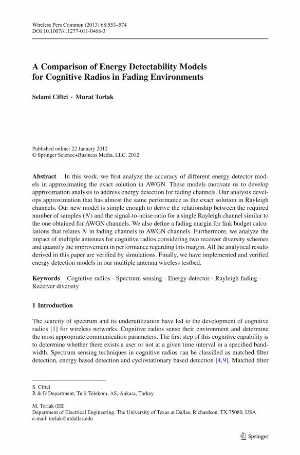
Fig. 1 Block diagram of energy detector

are given in Sect. 7. Section 8 is dedicated to verify our theoretical results via simulation andexperimental results and Sect. 9 concludes this work.

2 Review: Energy Based Spectrum Sensing in AWGN Channels

The spectrum sensing problem can be viewed as a binary detection problem. The binaryhypothesis testing considered in spectrum sensing can be given by

y(i) ={

n(i), H0

s(i)+ n(i), H1(1)

where H0 is null hypothesis and H1 is alternative hypothesis. The small bold letters representthe vector of length N in (1) which is equal to twice the time-bandwidth product (T W ).The noise samples n(i) is assumed to be additive white Gaussian noise with zero mean andvariance of σ 2

n . The primary signal samples s = [s(1), s(2), . . . , s(N )] are assumed to uncor-related to noise samples. The average primary signal power over N samples is Ps = ‖s‖2/N .In this paper, we focus on energy detection based method as illustrated in Fig. 1. Given Nreceived samples, the energy based detection solution for this problem is to find a decisionstatistic

� =N∑

i=1

|y(i)|2 (2)

and to compare it with a threshold λ. If� ≥ λ, the detector declares the presence of a primaryuser in the spectrum.

2.1 Exact Solution [6]

According to the exact solution, which is based on the work in [5], the received samples areGaussian random variables. When the signal exists, the decision statistic, �, is a noncen-tral χ2 random variable with N degrees of freedom and a noncentrality parameter, ρ. Thisparameter is equal to the ratio of signal energy measured over the sensing time to two-sidednoise spectral density. Throughout this paper, SNR is defined as the ratio of average primarysignal power to noise variance, SNR = Ps/σ

2n . Due to this, the relationship between ρ and

SNR is given by ρ = NSNR. When there is no signal in the energy detector’s input,� has acentral χ2 distribution with N degrees of freedom. The decision statistic in each hypothesescan be summarized as

� ={χ2

N , H0

χ2N (ρ), H1

(3)

123


where χ2m(η) is a χ2 variate with m degrees of freedom and a non-centrality parameter η.

The probability density function of the test statistic is

f�(�) ={

12N/2�(N/2)

�(N−2)/2e−�/2, H0

12

(�

NSNR

)(N−2)/4e−(�+NSNR)/2 I(N−2)/2(

√�NSNR), H1

(4)

where �(.) is the gamma function and Im(.) is the mth order modified Bessel function of thefirst kind.

Closed form expressions for probability of false-alarm, Pf , and probability of detection,Pd , in AWGN channels are computed as in [6,7] for the performance analysis of this energydetector. They are given by

Pf = �(N/2, λ/2)

�(N/2)

and Pd = QN/2(√

NSNR,√λ) (5)

where Qm(.) is the generalized Marcum Q-function [10].

2.2 Gaussian Approximation with Low SNR (Edell [3])

As the number of samples increases, N ≥ 20, the distribution of the test statistic under bothhypothesis converges to Normal distribution due to the Central Limit Theorem.

Edell [3] has exploited this feature in the radiometer problem and computed the mean, μ,and variance, σ 2, of the test statistic under both hypothesis. Thus, for large N , the statisticsof the decision variable, �, is modeled as

� ={N (

Nσ 2n , 2Nσ 4

n

)under H0

N (Nσ 2

n (1 + SNR), 2Nσ 4n

)under H1

(6)

For small SNR values (SNR << 1), the variances of the test statistic under both hypothesisare assumed to be equal to each other. According to this model, Pf and Pd can be written as

Pf = Q

(λ− N√

2N

)and Pd = Q

(λ− N (1 + SNR)√

2N

)(7)

where Q(.) is the well known tail probability of a zero-mean unit-variance Gaussian randomvariable; λ is the normalized threshold λ = λ/σ 2

n to satisfy the given Pf and Pd values. Therelationship between the number of samples, N , and SNR in AWGN channels for a givenPf and Pd is given by

N = 2(Q−1(Pf )− Q−1(Pd))2 SNR−2. (8)

This result is exactly the same with the one given in [2] except that the definition of SNR isdefined as the ratio of the total energy over sensing time and the noise variance. The requiredSNR can readily obtained from (8) as

SNRreq = √2[Q−1(Pf )− Q−1(Pd)

]/√

N (9)

123


2.3 Regular Gaussian Approximation

Regular Gaussian approximation as originally stated in [11] consider mean and variance ofthe test statistics without low SNR restriction:

� ={N (

Nσ 2n , 2Nσ 4

n

)under H0

N (Nσ 2

n (1 + SNR), 2Nσ 4n (1 + 2SNR)

)under H1

(10)

Using these values, Pf and Pd can be expressed as in (11) and (12).

Pf = Q

(λ− N√

2N (1 + 2SNR)

)(11)

Pd = Q

(λ− N (1 + SNR)√

2N (1 + 2SNR)

)(12)

The relationship between the required SNR and the number of samples N given Pd and Pf

be found as

SNRreq =√

2

N(β − ξ)+ 1

Nψ(β, ξ, N ) (13)

ψ(β, ξ, N ) = 2ξ2 − ξ√

2N

⎛⎝√

1 + 2ξ2

N+ 4β√

2N− 1

⎞⎠ (14)

where, β = Q−1(Pf ) and ξ = Q−1(Pf ). The N − SNR relationship in (13) is the same asthe one in [2] except that the SNR is defined as in Edell’s model.

2.4 Extended Berkeley Model

In this model, we build upon the approach taken in [9] which is referred as Berkeley Modelin this paper. Our extended approach may be the closest analytical approximation to the exactN − SNR relation established in 2 among the methods published in literature [2]. Berke-ley model applies Gaussian approximation to the log-likelihood ratio rather than signal andnoise samples directly. The details of this derivation can be found in [9]. Below we extend theBerkeley derivation. The log-likelihood ratio in the Neyman-Pearson test for the detectionproblem is given by

LLR(y(i)) =N∑

i=1

log

[Pr(y(i)|H1)

Pr(y(i)|H0)

]

=N∑

i=1

log

⎡⎢⎢⎢⎢⎣

∑Nn=1 pn

(1√

2πσ 2n

e− (y(i)−x(n))2

2σ2n

)

(1√

2πσ 2n

e− y(i)2

2σ2n

)

⎤⎥⎥⎥⎥⎦

:=N∑

i=1

f

(y(i)

σ 2n

)(15)

123


where f (t) := log[∑N

n=1 pn exp(− x(n)2

2σ 2n

− x(n)t)]

as defined in [9]. Based on the optimal

decision strategy

LLR(Y)H1≷H0

λ

and using CLT Pf and Pd are approximately evaluated as follows:

Pf = Q

⎛⎝λ− Nm0√

Nσ 20

⎞⎠ Pd = Q

⎛⎝λ− Nm1√

Nσ 21

⎞⎠ (16)

where

m0 = E

[f

(y(i)

σ 2n

)|H0

]σ 2

0 = Var

(f

(y(i)

σ 2n

)|H0

)(17)

m1 = E

[f

(y(i)

σ 2n

)|H1

]σ 2

1 = Var

(f

(y(i)

σ 2n

)|H1

)(18)

These equations are exactly the same to the one given in [9]. Since we need to find N −SNRrelation, we need to compute the quantities m0,m1, σ

20 , and σ 2

1 . In order to find these quan-

tities as a function SNR, the Berkeley model expands f(

y(i)σ 2

n

)using the Taylor series at 0

(due to low SNR assumption) to get

f (t) = log

[N∑

n=1

pne− x(n)2

2σ2n

−x(n)t]

(19)

≈N∑

n=1

pn

(x(n)t + x(n)2

2t2 + x(n)3

3! t3 + x(n)4

4! t4 + · · ·)

(20)

where t =(

y(i)σ 2

n

). Different from [9], we include terms up to the forth order in t to evaluate

the mean and variance quantities above more precisely as a function of SNR. Furthermore,for evaluating mean and variance, we only include terms up to SNR2 and SNR3, respectively.The higher order terms of SNR are neglected. We need the first four raw (sample) momentsof the primary signal to generate the approximated values above:

N∑n=1

pn x(n) = 0 (zero mean)N∑

n=1

pn x(n)2 = Ps (average power)

N∑n=1

pn x(n)3 ≈ 0N∑

n=1

pn x(n)4 ≈ 3P2s (21)

The third and fourth sample moments are approximated by assuming that the primary sig-nal follows Gaussian distribution up to fourth moment. If these moments are known for theprimary signal, they can be used to fine tune the approximation. Here, we now provide thekey results:

m1 − m0 = SNR2

2σ 2

0 = SNR2

2σ 2

1 = SNR2

2(5SNR + 1) (22)

123


102

103

104

105

−0.8

−0.7

−0.6

−0.5

−0.4

−0.3

−0.2

−0.1

0

Number of samples, N

Err

or (

dB)

in r

equi

red

SN

R fr

om e

xact

res

ults

Gaussian−Low SNRBerkeley/GaussianModified Berkeley

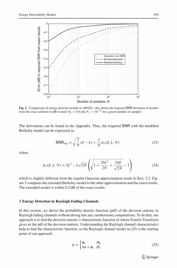
Fig. 2 Comparison of energy detector models in AWGN—this shows the required SNR deviation of modelsfrom the exact solution in dB to meet Pd = 0.9 and P f = 10−6 for a given number of samples

The derivations can be found in the Appendix. Thus, the required SNR with the modifiedBerkeley model can be expressed as

SNRreq =√

2

N(β − ξ)+ 1

Nψe(β, ξ, N ) (23)

where

ψe(β, ξ, N ) = 5ξ2 − ξ√

2N

⎛⎝√

1 + 25ξ2

2N+ 10β√

2N− 1

⎞⎠ (24)

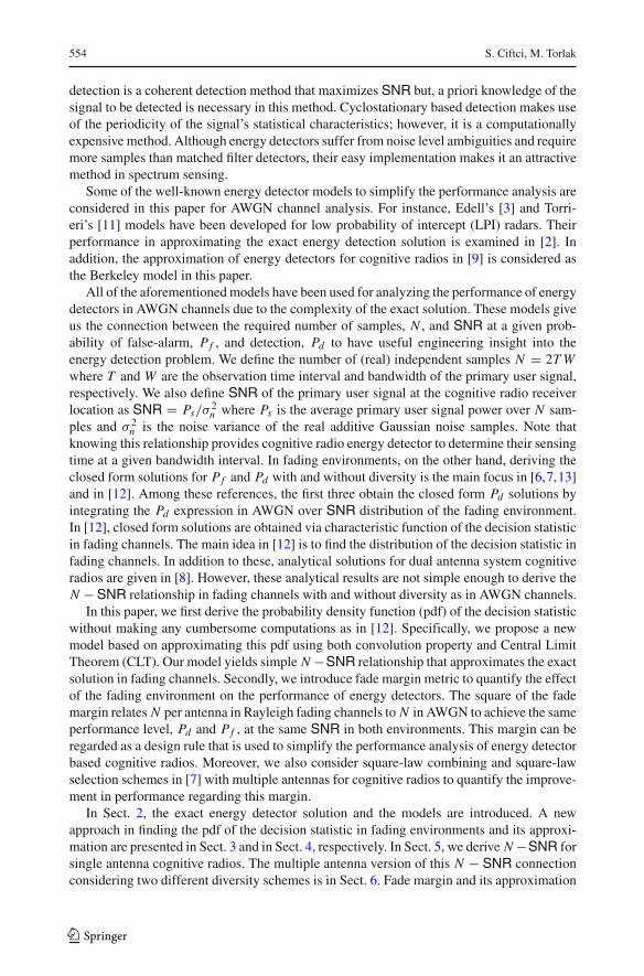
which is slightly different from the regular Gaussian approximation result in Sect. 2.3. Fig-ure 2 compares the extended Berkeley model to the other approximation and the exact results.The extended model is within 0.2 dB of the exact results.

3 Energy Detection in Rayleigh Fading Channels

In this section, we derive the probability density function (pdf) of the decision statistic inRayleigh fading channels without diving into any cumbersome computations. To do that, ourapproach is to find the decision statistic’s characteristic function of whose Fourier Transformgives us the pdf of the decision statistic. Understanding the Rayleigh channel characteristicshelp us find the characteristic function, so the Rayleigh channel model in (25) is the startingpoint of our approach.

y ={

n, H0

hs + n, H1(25)

123


In this model, bold letters represent a complex vector of length u that is half the total numberof samples, N . Here, the vector n contains the noise samples whereas s is the deterministicsignal vector. The complex variable h is the channel coefficient and it is assumed to be acomplex Gaussian variable with zero mean and unit variance for Rayleigh channels.

In AWGN channels, the decision statistic’s characteristic function is determined intuitivelyby the elements of received y vector. Since y is multivariate complex Gaussian distributedbecause of the statistics of the received samples, the distribution of the absolute square ofthem is either central or non-central χ2. In this way, we can easily write the characteristicfunction of the decision statistic. In any fading channels, we do not need to find the charac-teristic function of the decision statistic under null hypothesis because it is just noise. Thus,it is the characteristic function of the summation of random variables each of which has acentral χ2 distribution of degree 2. To determine it under alternative hypothesis in Rayleighfading channels intuitively, we apply a Householder Transformation to y under alternativehypothesis. Due to linearity of this transformation, transforming y vector means to transformhs and n. According to the Rayleigh channel model in (25), the samples of deterministic s arein every dimension of signal space. There exists a Householder transformation that makesall the deterministic samples lie in one dimension. This transformation matrix is of the formin (26) as given in [15].

U = I − zzH

zH a(26)

where a,b ∈ Cu . The z vector is given by z = a − b where a and b in our case are given by

a = hs and b = ‖a‖[1 0 . . . 0]T (27)

The circularly n vector exposed to this transformation preserves its characteristics. The illus-tration of this process is in the following.

y = Uy = hUs + Un (28)

=√

|h|2 Es

⎡⎢⎢⎢⎣

10...

0

⎤⎥⎥⎥⎦ +

⎡⎢⎢⎣...

n...

⎤⎥⎥⎦ (29)

The transformed y vector is now composed of u − 1 circularly Gaussian distributed noisesamples with zero mean and unit variance and one circularly Gaussian distributed samplewith zero mean and variance equal to 2σ 2

n + Es . Since the Householder Transformation is anorm preserving unitary transformation, the decision statistic is nothing but the sum of theabsolute square of the elements of y. Hence, the decision statistic is the sum of u − 1 centralχ2 distributed variables of degree 2 of 2σ 2

n variance and one central χ2 distributed variableof degree 2 whose variance is 2σ 2

n (1 + uSNR). To summarize, the characteristic function ofthe decision statistic under both hypothesis is given in (30).

( jw) =⎧⎨⎩(1 − 2 jwσ 2

n )−u, H0

(1 − 2 jwσ 2n )

1−u

1 − j2wσ 2n (1 + uSNR)

, H1(30)

In this way, we obtain the characteristic function of the decision statistic without applying anycumbersome computations as in [12]. Similarly, the characteristic function of the decisionstatistic in AWGN channels is also obtained by assuming h is a deterministic. In this case,

123


it is either the characteristic function of central χ2 or that of noncentral χ2 as summarizedin (31).

(

jw | |h|2) ={(1 − 2 jwσ 2

n )−u, H0

(1 − 2 jwσ 2n )

−u exp(

jwu|h|2SNR1/(2σ 2

n )− jw

), H1

(31)

The pdf of the decision statistic in Rayleigh channels is obtained by taking the FourierTransform of the characteristic function in (30). False alarm and detection probabilities inRayleigh channels are computed by integrating above pdfs of the decision statistic from athreshold value to infinity:

P f = �(u, λ/(2σ 2n ))

�(u)(32)

Pd = exp

(− λ

2σ 2n

) u−2∑n=0

1

�(n + 1)

(λ

2σ 2n

)n

+(σ 2

n + SNRSNR

)u−1

×[

exp

(− λ

2(σ 2n + SNR)

)− exp

(− λ

2σ 2n

) u−2∑n=0

1

�(n + 1)

(λSNR

2(σ 2n + SNR)

)n]

(33)

where u = N/2 and λ is the threshold to satisfy the given Pf and Pd values. Since linearfunctions of N are in the boundaries of the summation terms in (32), it is not possible toderive a simple N −SNR relationship for Rayleigh channels using the exact energy detectorsolution. Due to this, we propose an approximate energy detector model for Rayleigh fadingchannels based on approximating the pdf of the decision statistic.

4 Approximation of the Energy Detection Statistics in Fading

Since all those energy detector models in AWGN channels are based on approximating thedistribution of the decision statistic via Central Limit Theorem (CLT), we need to invokeCLT for the decision statistic in Rayleigh fading channels to see the applicability of thesemodels to Rayleigh fading channels. To do that, we consider the sum of absolute square ofeach element in y. Classical CLT states that the sum of a large number of independent andidentically distributed random variables is approximated by normal distribution if they havefinite variances. The sum of independent variables is approximated by CLT if they satisfyLyapunov’s condition [14]. However, the random variables summed in the equation of thedecision statistic do not satisfy this condition. However, we rewrite the decision statistic interms of y as

�r = yH y = |y1|2 +u∑

i=2

|yi |2 = Y1 +u∑

i=2

Yi . (34)

where u = N/2. The mean and variance of χ2 distributed Yi ’s are

μi ={

2σ 2n (1 + uSNR), i = 1

2σ 2n , i = 2, . . . , u

and (35)

σ 2Yi

={

4σ 4n (1 + uSNR)2, i = 1

4σ 4n , i = 2, . . . , u

(36)

123


If we consider the sum of Yi ’s for i = 2, . . . , u as a single χ2 distributed random variable,its mean and variance is

Z =u∑

i=2

Yi ⇒ μZ = 2(u − 1)σ 2n and σ 2

Z = 4(u − 1)σ 4n . (37)

The variance of Y1 is much much greater than that of Z for large sample size values becauseσ 2

Y1is proportional to u2 whereas σ 2

Z is proportional to u.The probability density function and hence, Pd equation is very complicated. Our aim is to

find a simplified version of Pd . For large sample sizes, Central Limit Theorem is the very firstsolution to this kind of problems but, it doesn’t work in this case as shown in Appendix. Thereason is that the variance of one of the summed terms dominates the variance of the decisionstatistic. Our approach for this case is based on the convolution property. Since the decisionstatistic is nothing but the sum of independent random variables, its pdf is the convolutionof the summed terms’ pdfs. Since σ 2

Y1>> σ 2

Z for large sample sizes, the variance of thedecision statistic is approximated to be equal to the variance of Y1. The mean value, however,is the sum of the summed terms’ mean values. This idea can be illustrated by considering theconvolution of any continuous function with delta dirac function. Thus, our approximatedpdf of the decision statistic for a single antenna case becomes

f�r (�r ) = 1

2σ 2n (1 + uSNR)

exp

(−�r/σ

2n − 2(u − 1)

2(1 + uSNR)

)for �r ≥ 2(u − 1)σ 2

n (38)

5 N-SNR Relation in Fading Channels

Our goal is to derive an approximated N − SNR relation under Rayleigh fading. First, recallPf which is already approximated in 7. Then, Pd for a single antenna cognitive radios canbe computed by integrating (38) from a threshold to infinity as

Pd =∞∫

λ,λ≥2(u−1)σ 2n

1

2σ 2n (1 + uSNR)

exp

(−�r/σ

2n − 2(u − 1)

2(1 + uSNR)

)d�r (39)

We rewrite the threshold value in (39) from (7) as

λ

σ 2n

= 2u + 2√

u Q−1(Pf ). (40)

Then, substituting this value into (39) yields

Pd = exp

(−

√uβ + 1

1 + uSNR

)where β = Q−1(Pf ). (41)

From (41), we obtain the following quadratic equation.

− log(Pd)SNR u − β

√u − (1 + log

(Pd)) = 0 (42)

By neglecting non-dominating terms (i.e., O(1/SNR)) in the exact solution of (42), we obtainour desired N − SNR expression for Nr = 2u as in (49).

Nr =(

β

− log(Pd))2

2

SNR2 (43)

123


The beauty of the expression in (43) is that it depends only on Pf and Pd , which are thepredetermined values for system design.

6 N − SNR Relationship in Multi-Antenna Energy Detection

In this section, we consider that there are multiple antennas in cognitive radios and each ofthem sense the same spectrum based on energy detection in fading environments. Our focusis to understand how multiple antennas in cognitive radios, each of which employs energydetector, advance their spectrum sensing performance. We consider two different combiningschemes for cognitive radios in this section. The first one is the square-law combining andthe other one is square-law selection. The exact expression both methods are already derivedin [7].

As with the single antenna case, we derive the N − SNR relationship at a specified Pd

and Pf for any number of antennas for these techniques.

6.1 Square-Law Combining (SLC)

The first combining technique is Square-Law Combining technique in which the outputof each antenna’s energy detector is added. The cognitive radio decides whether there isa primary user or not by comparing the output of this summation to a threshold value. Inthis way, the decision statistic is nothing but the sum of the outputs of each antenna. Theapproximated pdf of the decision statistic for L antennas in this scheme is of the form

f�SLC (�SLC ) =(�SLC/σ

2n − 2L(u − 1)

)L−1

(2(1 + uSNR))L (L − 1)! exp

(−�SLC/σ

2n − 2L(u − 1)

2(1 + uSNR)

). (44)

Pd,SLC is found to be

Pd,SLC = 1

�(L)�

(L ,λ/σ 2

n − 2L(u − 1)

2(1 + uSNR)

)(45)

where λ is the threshold which is again calculated from a specified Pf,SLC . Using thedefinition of regularized incomplete gamma function, we can also express Pd,SLC as

Pd,SLC = P

(L ,λ/σ 2

n − 2L(u − 1)

2(1 + uSNR)

)where P(a, z) = �(a, z)

�(a). (46)

With CLT approximation for the distribution of the decision statistic for L antennas, P f,SLC

is approximated as

P f,SLC = Q

(λ/σ 2

n − 2Lu

2√

Lu

)(47)

Obtaining the threshold value from (47) and substituting it to (46) yields the quadraticequation in (48).

P−1 (L , Pd,SLC)

SNR u − β√

L√

u − (L − P−1 (L , Pd,SLC)) = 0 (48)

The desired N − SNR expression for L i.i.d. antennas with SLC scheme is in (49).

NSLC =(

β√

L

P−1(L , Pd,SLC

))2

2

SNR2 (49)

As expected, (49) is equivalent to (43) for L = 1.

123


6.2 Square-Law Selection (SLS)

In this scheme, the decision statistic is the output of one of the energy detectors that has thehighest energy. The outputs of each antenna’s energy detector is compared and the highestone is selected via a switch. The decision whether there is a primary user or not is made bycomparing the selected antenna’s output with a threshold value.

Similar to the analysis for SLC scheme, the probability of false alarm is represented byPf,SL S and the probability of detection is represented by Pd,SL S for multiple antennas inRayleigh fading channels. As in SLC scheme, we have the same i.i.d channel assumption inthe analysis here.

Let L be the number of antennas, P f,SL S is given by

Pf,SL S = 1 − (1 − P f

)L(50)

where Pf is defined in (7). Assuming that the average SNR is equal for each branch of LRayleigh channels, Pd,SL S is given by

Pd,SL S = 1 − (1 − Pd

)L. (51)

With little manipulation of (51) and using (46), we obtain

1 − L√

1 − Pd,SL S = P

(1,λ/σ 2

n − 2(u − 1)

2(1 + uSNR)

). (52)

This equation yields a quadratic equation. Making some assumptions, which we have done forboth single antenna and multi-antenna with SLC scheme cases, helps us solve that quadraticform for γSL S . This solution gives us the desired N − SNR relationship as

NSL S =

⎛⎜⎜⎝ β

− log

(1, 1 − L

√1 − Pd,SL S

)⎞⎟⎟⎠

2

2

SNR2 (53)

where β = Q−1((

1 − L√

1 − P f

)).

7 Fade Margin

We introduce the fade margin to quantify the effect of the fading environment on the perfor-mance of energy detectors. The fade margin for SNR is the factor that relates the requiredaverage SNR per antenna in Rayleigh fading channels to the required SNR in AWGN toachieve the same performance level by taking the same number of samples in both environ-ments. Let us consider the following scenario. Assume that we know the required SNR inAWGN to achieve some given Pf and Pd values by taking N samples. Our aim is to find therequired average SNR in Rayleigh fading channels to achieve the same Pf and Pd with thesame number of samples.

In order to obtain the fade margin, we make use of N − SNR relationship given in (43).The assumption of fixing P f (Pf in AWGN), Pd (Pd in AWGN) and N values and N =Nawgn = Nray . These assumptions allows us to replace the term Nr in (43) by the righthand side of the equation in (8). Thus, we define fade margin (F) as the ratio between the

123


required SNRs in Rayleigh and AWGN channels for energy detection with fixed observationintervals:

F = SNRR

SNRA= β

(β − ξ))

(1

log (Pd)

). (54)

where SNRR and SNRA are the required SNRs in Rayleigh and AWGN channels, respec-tively. Here, our fade margin is nothing but

γF =(

β

β − ξ

)(1

k

). (55)

where k = − ln (Pd). Similarly, we can also define a factor for some number of samplesthat relates the required number of samples per antenna in Rayleigh fading channels to therequired number of samples in AWGN to achieve the same performance level at the sameSNR values in both environments. In this case, one can calculate how many samples he needsto achieve the same performance in Rayleigh fading environment as compared to AWGNenvironment. Using a similar approach to fade margin, we start from (43) and replace theaverage SNR term with the one in (8) based on our Pf and Pd . In this way, we obtain thefactor which is nothing but the square of our fade margin given in (56).

NF =(

β

β − ξ

)2 (1

− log(Pd)

)2

(56)

A more generalized version of this margin can be obtained by considering cognitive radioswith multiple antennas. Following the same steps we take for single antenna case, the fademargin for multi-antenna SLC case is obtained by using (8) and (49) as

γF,slc =(

β

β − ξ

)(1

�−1 (L , Pd)

)(57)

Similarly, the fade margin for multi-antenna SLS case is obtained by using (8) and (53) as

γF,sls =(

β

β − ξ

)(1

− log(1, 1 − L

√1 − Pd

))

(58)

After finding this margin for multiple antenna systems, we will try to demonstrate how usefulthis margin is from a system designer perspective. Assume that we know the required numberof samples per antenna, N1, for a single antenna in Rayleigh fading environment for givenPd , Pf and average SNR values. We wonder how few number of samples per antenna isrequired when we increase the number of antennas from 1 to L . Assume that the requirednumber of samples for L antennas is NL . So,

NL = N1 × fading factor for L antennas

fading factor for a single antenna(59)

Consider using SLC scheme for multiple antenna case. Thus, (59) becomes

NL = N1 ×⎛⎝

ββ−ξ

1�−1(L ,Pd )

ββ−ξ

1�−1(1,Pd )

⎞⎠

2

= N1 ×(�−1(1, Pd)

�−1(L , Pd)

)2

(60)

123


where β = erfc−1(2Pf ) and ξ = erfc−1(2Pd). Using SLS scheme, a similar version of (60)is obtained:

NL = N1 ×(�−1

(1, 1 − 1

√1 − Pd

)�−1

(1, 1 − L

√1 − Pd

))2

(61)

We make the following definitions for our purposes in this section:NF,slc: The ratio between the required number of samples (Nreq ) per antenna for L

antennas and that for a single antenna with SLCscheme at fixed Pd , Pf and SNR.

NF,sls : The ratio between the Nreq per antenna for L antennas and that for a singleantenna with SLSscheme at fixed Pd , Pf and SNR.

γF,slc: The ratio between the required SNR per antenna for L antennas and that for asingle antenna with SLCscheme at fixed Pd , Pf and number of samples.

γF,sls : The ratio between the required SNR per antenna for L antennas and that for asingle one with SLSscheme at fixed Pd , Pf and number of samples.

The mathematical expressions for NF,slc and NF,sls are given in (62).

NF,slc =(

P−1(1, Pd)

P−1(L , Pd)

)2

NF,sls =(

P−1(1, 1 − 1

√1 − Pd

)P−1

(1, 1 − L

√1 − Pd

))2

(62)

The expressions for γF,slc and γF,sls is the square root of the ones in (62).

γF,slc = P−1(1, Pd)

P−1(L , Pd)and γF,sls = P−1

(1, 1 − 1

√1 − Pd

)P−1

(1, 1 − L

√1 − Pd

) (63)

All of these expressions are nothing but a ratio of two inverse of upper incomplete gammafunctions. Since this function is not used as frequently as any other function like rational orpower functions, it is really difficult to get an intuition how the value of NF,slc or the otherones change. Therefore, a simplified expression for inverse of upper incomplete gamma func-tion can be obtained by using the findings of [16]. In [16], the connection of lower incompletegamma function with confluent hypergeometric function [17] is established as

g(a, x) = xa

a× 1 F1(a, 1 + a,−x) (64)

where g(., .) is the lower incomplete gamma function and 1 F1(a, 1 + a,−x) is the conflu-ent hypergeometric function. As x → 0,1 F1(a, 1 + a,−x) → 1 and the inverse of lowerincomplete gamma function is given by

g−1(a, x) = a√

ax (65)

Benefiting from the above approximation, we express the upper incomplete gamma functionin our expressions in terms of lower incomplete gamma function. By definition, upper andlower incomplete gamma functions satisfy

�(a, x) = �(a)− g(a, x). (66)

123


Using (66), we rewrite (45) and (52) as

1 − Pd,slc = 1

�(L)g

(L ,

2 γslc β√

Nslc − 1

(γslc)2 Nslc

)

L√

1 − Pd,sls = g

(1,

2 (γsls)√

Nsls β − 1

Nsls (γsls)2

)(67)

With these representations, the expressions for the new definitions in this section can berewritten as

NF,slc =(

g−1(1, 1 − Pd)

g−1(L , 1 − Pd)

)2

NF,sls =(

g−1(1, 1

√1 − Pd

)g−1

(1, L

√1 − Pd

))2

(68)

γF,slc = g−1(1, 1 − Pd)

g−1(L , 1 − Pd)

γF,sls = g−1(1, 1

√1 − Pd

)g−1

(1, L

√1 − Pd

) . (69)

As Pd → 1, (1 − Pd) → 0 and these inverse functions can be approximated by (65).Hence, (68) and (69) can be expressed as

NF,slc ≈ 1

�(L + 1)2L

(1 − Pd)2(1− 1

L )

NF,sls ≈ (1 − Pd)2(1− 1

L ) (70)

γF,slc ≈ 1

�(L + 1)1L

(1 − Pd)1− 1

L

γF,sls ≈ (1 − Pd)1− 1

L . (71)

8 Simulation and Experimental Results

In the simulations, we compare our proposed energy detector model with the exact solutionand figure out how well it approximates the exact solution in Rayleigh channels. All the sim-ulations are evaluated in Mathematica to get accurate results. We also use the fading factorfor SNR and required number of samples to find the required SNR and N in Rayleigh fadingchannels and compare these values with exact values. We also show how our fading factorbehaves as Pd varies.

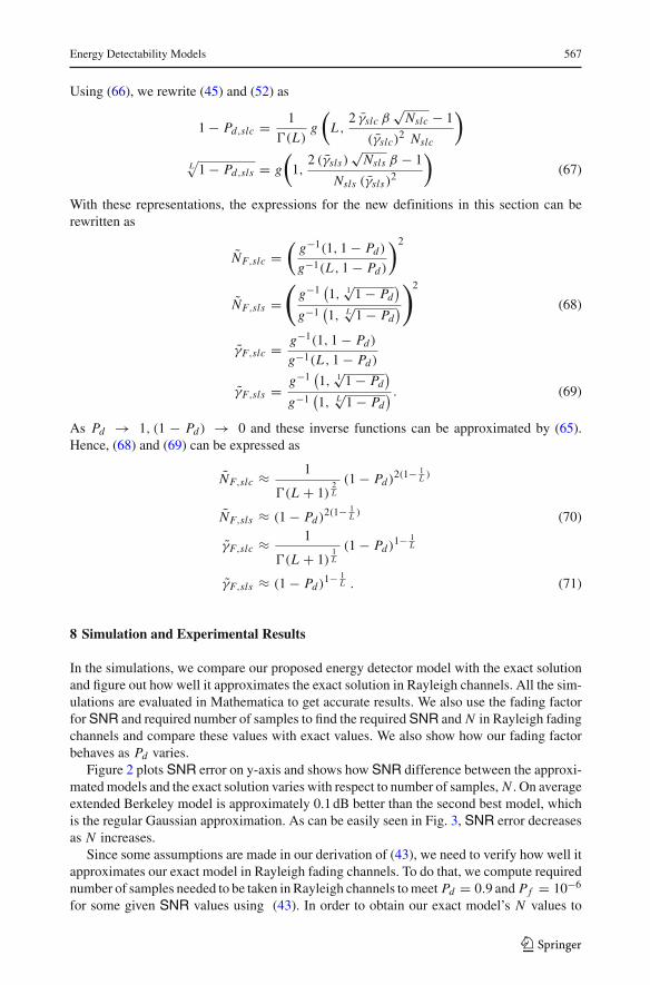
Figure 2 plots SNR error on y-axis and shows how SNR difference between the approxi-mated models and the exact solution varies with respect to number of samples, N . On averageextended Berkeley model is approximately 0.1 dB better than the second best model, whichis the regular Gaussian approximation. As can be easily seen in Fig. 3, SNR error decreasesas N increases.

Since some assumptions are made in our derivation of (43), we need to verify how well itapproximates our exact model in Rayleigh fading channels. To do that, we compute requirednumber of samples needed to be taken in Rayleigh channels to meet Pd = 0.9 and Pf = 10−6

for some given SNR values using (43). In order to obtain our exact model’s N values to

123


0.1 0.2 0.3 0.4 0.5 0.6 0.7 0.8 0.9−4

−2

0

2

4

6

8

10

Pd

Fad

ing

Fac

tor

1 antenna

2 antennas

3 antennas

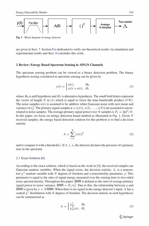
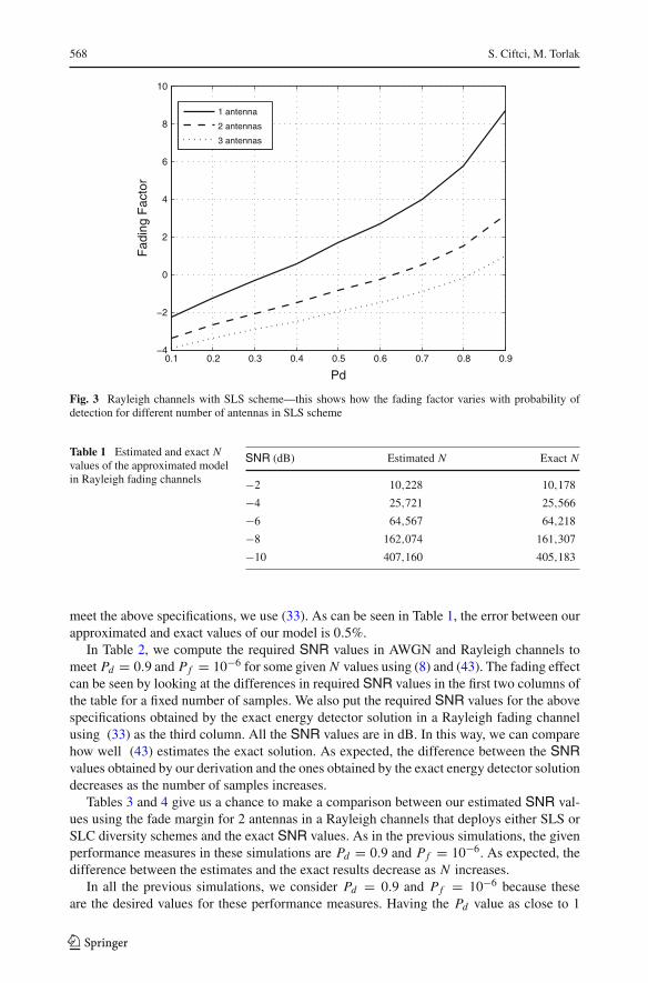
Fig. 3 Rayleigh channels with SLS scheme—this shows how the fading factor varies with probability ofdetection for different number of antennas in SLS scheme

Table 1 Estimated and exact Nvalues of the approximated modelin Rayleigh fading channels

SNR (dB) Estimated N Exact N

−2 10,228 10,178

−4 25,721 25,566

−6 64,567 64,218

−8 162,074 161,307

−10 407,160 405,183

meet the above specifications, we use (33). As can be seen in Table 1, the error between ourapproximated and exact values of our model is 0.5%.

In Table 2, we compute the required SNR values in AWGN and Rayleigh channels tomeet Pd = 0.9 and Pf = 10−6 for some given N values using (8) and (43). The fading effectcan be seen by looking at the differences in required SNR values in the first two columns ofthe table for a fixed number of samples. We also put the required SNR values for the abovespecifications obtained by the exact energy detector solution in a Rayleigh fading channelusing (33) as the third column. All the SNR values are in dB. In this way, we can comparehow well (43) estimates the exact solution. As expected, the difference between the SNRvalues obtained by our derivation and the ones obtained by the exact energy detector solutiondecreases as the number of samples increases.

Tables 3 and 4 give us a chance to make a comparison between our estimated SNR val-ues using the fade margin for 2 antennas in a Rayleigh channels that deploys either SLS orSLC diversity schemes and the exact SNR values. As in the previous simulations, the givenperformance measures in these simulations are Pd = 0.9 and Pf = 10−6. As expected, thedifference between the estimates and the exact results decrease as N increases.

In all the previous simulations, we consider Pd = 0.9 and Pf = 10−6 because theseare the desired values for these performance measures. Having the Pd value as close to 1

123


Table 2 Required SNR valuesin AWGN and Rayleigh channelsfor a single antenna

N SNR using (8) SNR using (57) SNR using (33)

200 −2.1932 6.5433 7.2333

500 −4.1829 4.5536 4.9959

1,000 −5.6881 3.0484 3.3617

1,500 −6.5686 2.168 2.4232

2,000 −7.1932 1.5433 1.7636

Table 3 Required SNR valuesin AWGN and Rayleigh channelswith 2 SLS antennas


200 −2.1932 0.970733 1.6202

500 −4.1829 −1.01897 −0.6005

1,000 −5.6881 −2.57096 −2.248

1,500 −6.5686 −3.40456 −3.1902

2,000 −7.1932 −4.02926 −3.841

Table 4 Required SNR valuesin AWGN and Rayleigh channelswith 2 SLC antennas


200 −2.1932 1.0176 1.615

500 −4.1829 −0.9721 −0.655

1,000 −5.6881 −2.4772 −2.11

1,500 −6.5686 −3.3577 −3.061

2,000 −7.1932 −3.9824 −3.6415

provides the secondary user with cognitive radios not to interfere the primary users by highdetection probability. However, we consider the fading factor for different Pd values in orderto see how it is affected by Pd values. The simulation results to exploit how fading factorvaries with Pd values are given in Fig. 3 and (57) depending on the diversity scheme. Notsurprisingly, fading factor increases as Pd increases. Similarly, the variation in fading factorvalues decreases as the number of antennas increases. This is expected because the fadingfactor is calculated with respect to SNR values in AWGN and as the number of antennasincrease, the fading effect on system decreases and gets closer to AWGN system. It is alsoseen that the variation in the SLC results are more than those in SLS results.

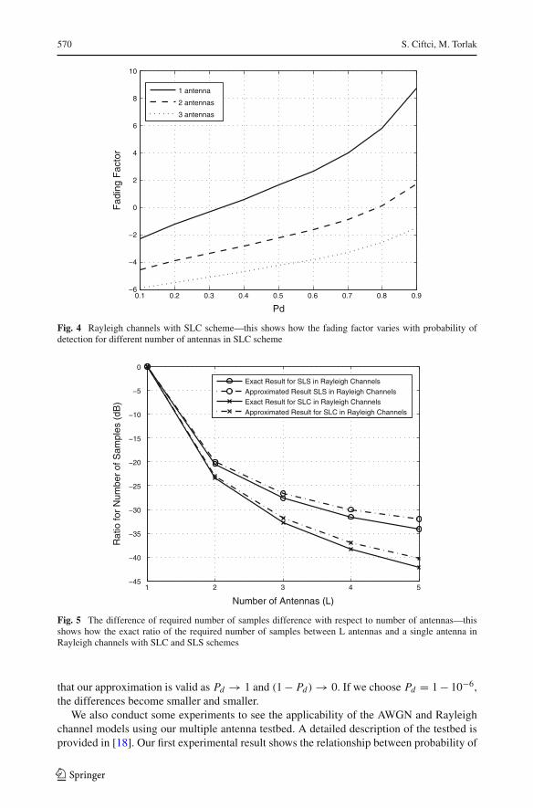
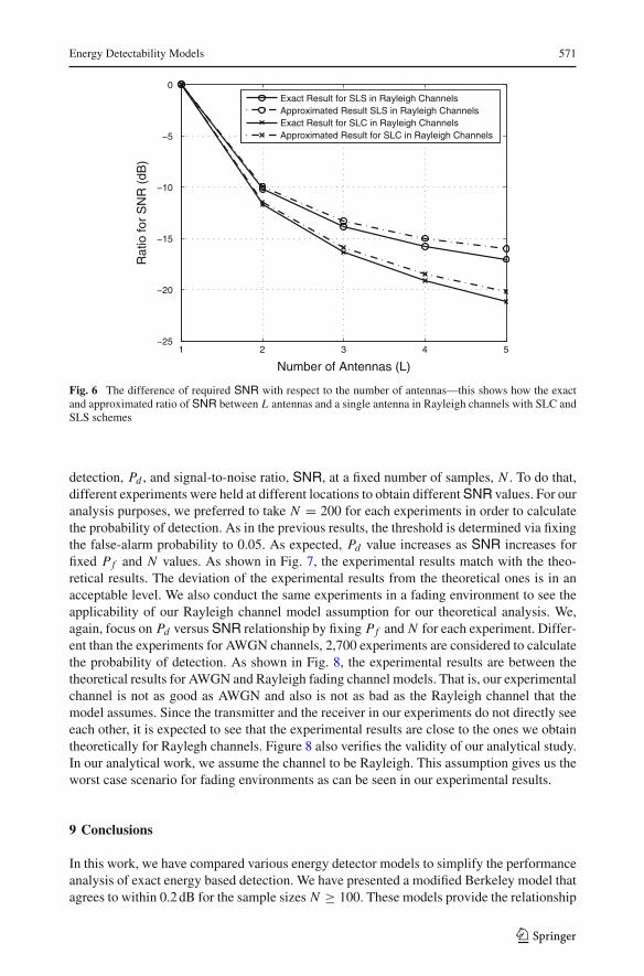
We demonstrate how the exact ratio of the required number of samples per antenna betweenL antennas and a single antenna varies for both SLC and SLS schemes in (5). As given inSect. 7, the exact expression is the ratio of two inverse-incomplete gamma functions. Theapproximated ratios, which are given in (70), are also plotted in Figs 4 and 5 to show howclose they approximate the exact solution. We also plot the variation of the same ratio forSNR in Fig. 6. As expected, the differences between consecutive number of antennas withSLC and that with SLS decrease as the number of antennas in the system increases. As thecollaborated antennas increase, the strength of SLC scheme over SLS scheme becomes moreobvious. On the other hand, the differences between the exact ratio and approximated ratiodoes not seem to get closer as the number of antennas increases. The reason behind this is

123


0.1 0.2 0.3 0.4 0.5 0.6 0.7 0.8 0.9−6

−4

−2

0

2

4

6

8

10

Pd

Fad

ing

Fac

tor

1 antenna

2 antennas

3 antennas

Fig. 4 Rayleigh channels with SLC scheme—this shows how the fading factor varies with probability ofdetection for different number of antennas in SLC scheme

1 2 3 4 5−45

−40

−35

−30

−25

−20

−15

−10

−5

0

Number of Antennas (L)

Rat

io fo

r N

umbe

r of

Sam

ples

(dB

)

Exact Result for SLS in Rayleigh ChannelsApproximated Result SLS in Rayleigh ChannelsExact Result for SLC in Rayleigh ChannelsApproximated Result for SLC in Rayleigh Channels

Fig. 5 The difference of required number of samples difference with respect to number of antennas—thisshows how the exact ratio of the required number of samples between L antennas and a single antenna inRayleigh channels with SLC and SLS schemes

that our approximation is valid as Pd → 1 and (1 − Pd) → 0. If we choose Pd = 1 − 10−6,the differences become smaller and smaller.

We also conduct some experiments to see the applicability of the AWGN and Rayleighchannel models using our multiple antenna testbed. A detailed description of the testbed isprovided in [18]. Our first experimental result shows the relationship between probability of

123


1 2 3 4 5−25

−20

−15

−10

−5

0

Number of Antennas (L)

Rat

io fo

r S

NR

(dB

)

Exact Result for SLS in Rayleigh ChannelsApproximated Result SLS in Rayleigh ChannelsExact Result for SLC in Rayleigh ChannelsApproximated Result for SLC in Rayleigh Channels

Fig. 6 The difference of required SNR with respect to the number of antennas—this shows how the exactand approximated ratio of SNR between L antennas and a single antenna in Rayleigh channels with SLC andSLS schemes

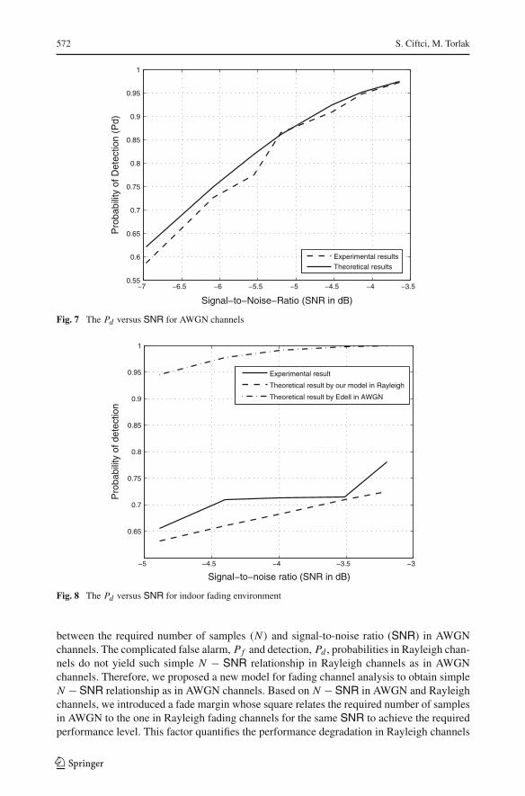
detection, Pd , and signal-to-noise ratio, SNR, at a fixed number of samples, N . To do that,different experiments were held at different locations to obtain different SNR values. For ouranalysis purposes, we preferred to take N = 200 for each experiments in order to calculatethe probability of detection. As in the previous results, the threshold is determined via fixingthe false-alarm probability to 0.05. As expected, Pd value increases as SNR increases forfixed Pf and N values. As shown in Fig. 7, the experimental results match with the theo-retical results. The deviation of the experimental results from the theoretical ones is in anacceptable level. We also conduct the same experiments in a fading environment to see theapplicability of our Rayleigh channel model assumption for our theoretical analysis. We,again, focus on Pd versus SNR relationship by fixing Pf and N for each experiment. Differ-ent than the experiments for AWGN channels, 2,700 experiments are considered to calculatethe probability of detection. As shown in Fig. 8, the experimental results are between thetheoretical results for AWGN and Rayleigh fading channel models. That is, our experimentalchannel is not as good as AWGN and also is not as bad as the Rayleigh channel that themodel assumes. Since the transmitter and the receiver in our experiments do not directly seeeach other, it is expected to see that the experimental results are close to the ones we obtaintheoretically for Raylegh channels. Figure 8 also verifies the validity of our analytical study.In our analytical work, we assume the channel to be Rayleigh. This assumption gives us theworst case scenario for fading environments as can be seen in our experimental results.

9 Conclusions

In this work, we have compared various energy detector models to simplify the performanceanalysis of exact energy based detection. We have presented a modified Berkeley model thatagrees to within 0.2 dB for the sample sizes N ≥ 100. These models provide the relationship

123


−7 −6.5 −6 −5.5 −5 −4.5 −4 −3.50.55

0.6

0.65

0.7

0.75

0.8

0.85

0.9

0.95

1

Pro

babi

lity

of D

etec

tion

(Pd)

Signal−to−Noise−Ratio (SNR in dB)

Experimental resultsTheoretical results

Fig. 7 The Pd versus SNR for AWGN channels

−5 −4.5 −4 −3.5 −3

0.65

0.7

0.75

0.8

0.85

0.9

0.95

1

Pro

babi

lity

of d

etec

tion

Signal−to−noise ratio (SNR in dB)

Experimental result

Theoretical result by our model in Rayleigh

Theoretical result by Edell in AWGN

Fig. 8 The Pd versus SNR for indoor fading environment

between the required number of samples (N ) and signal-to-noise ratio (SNR) in AWGNchannels. The complicated false alarm, Pf and detection, Pd , probabilities in Rayleigh chan-nels do not yield such simple N − SNR relationship in Rayleigh channels as in AWGNchannels. Therefore, we proposed a new model for fading channel analysis to obtain simpleN − SNR relationship as in AWGN channels. Based on N − SNR in AWGN and Rayleighchannels, we introduced a fade margin whose square relates the required number of samplesin AWGN to the one in Rayleigh fading channels for the same SNR to achieve the requiredperformance level. This factor quantifies the performance degradation in Rayleigh channels

123


as compared to AWGN channels. The improvement in the performance of cognitive radioswith multiple antennas is measured via fade margin. Simulation results coincide with exper-imental results done with the experimental multiple antenna testbed in indoor environment.The closeness of the simulation and experimental results shows that this margin is promisingin reducing the time spent on cognitive radio design.

Appendix: Derivation of (22)

Following the derivation steps in [9], we approximate f (t) at t = y(i)/σ 2n ≈ 0 using

Eqs. (20) and (21):

f

(y(i)

σ 2n

)≈ SNR

2

y(i)2

σ 2n

+ 3SNR2

4!y(i)4

σ 4n

(72)

Using the above approximation and ignoring the last term for m0 and m1, we have

m0 = E( f (t)|H0) ≈ SNR2

E(y(i)2|H0)

σ 2n

= SNR2

. (73)

Similarly, we have

m1 = E( f (t)|H1) ≈ SNR2

E(y(i)2|H1)

σ 2n

= SNR(1 + SNR)2

. (74)

Similar calculations for variances are obtained

σ 20 = E( f (t)2|H0)− m2

0 ≈ SNR2

2 . (75)

σ 21 = E(( f (t)2|H1)− E(( f (t)|H1)

2 ≈ SNR2(1+5SNR)2

using

E(( f (t)2|H1) = SNR2

4σ 4n

E(y(i)4|H1)+ 3SNR3

4!σ 6n

E(y(i)6|H1)+ h.o.t.

≈ SNR2(3σ 2n + 6Psσ

2n + h.o.t)

4σ 4n

+ 3SNR3(15σ 2n + h.o.t.)

24σ 6n

≈ SNR2(3 + 6SNR)4

+ 15SNR3

8

and

E(( f (t)|H1)2 =

(SNR(1 + SNR)

2+ 3SNR3(3σ 4

n + h.o.t.)

4!σ 4n

)2

≈ SNR2(1 + 2SNR)4

+ 9SNR3

24

References

1. Mitola, J., III. (1999). Cognitive radio for flexible mobile multimedia communication. In Proceedingsof IEEE International Workshop on Mobile Multimedia Communications (pp. 3–10).

2. Mills, R. F., & Prescott, G. E. (1996). A comparison of various radiometer detection models. IEEETransactions on Aerospace and Electronic Systems, 32(1), 467–473.

123


3. Edell, J. (1976). Wideband, noncoherent, frequency-hopped waveforms and their hybrids in low-prob-ability of intercept communications. Report Naval Research Laboratory (NRL) 8025.

4. Akyildiz, I. F., Lee, W. Y., Vuran, M. C., & Mohanty, S. (2006). NeXt generation/dynamic spec-trum access/cognitive radio wireless networks: A survey. Computer Networks Journal (Elsevier), 50,2127–2159.

5. Urkowitz, H. (1967). Energy detection of unknown deterministic signals. Proceedings of IEEE, 55,223–231.

6. Digham, F. F., Alouini, M. S. & Simon, M. K. (2003). On the energy detection of unknown signalsover fading channels. In Proceedings of IEEE (pp. 3575–3579).

7. Digham, F. F., Alouini, M. S. & Simon M. K. (2007). On the energy detection of unknown signalsover fading channels. IEEE Transactions on Communications, 55(1), 21–24.

8. Pandharipande, A. & Linnartz, J.-P. M. G. (2007). Performance analysis of primary user detec-tion in a multiple antenna cognitive radio. In IEEE International Conference on Communications(pp. 6482–6486).

9. Cabric, D., Tkachenko, A. & Brodersen, R. W. (2006). Experimental study of spectrum sensing beasedon energy detection and network cooperation. In Proceedings on ACM International workshop onTechnology and Policy for Accessing Spectrum.

10. Nuttall, A. H. (1975). Some integrals involving the QM function. IEEE Transactions on InformationTheory, 21, 95–96.

11. Torrieri, D. J. (1992). Principles of secure communication systems. Boston, MA: Artech House.12. Kostylev, V. I. (2002). Energy detection of a signal with random amplitude. IEEE International

Conference on Communications, ICC 2002, 3, 1606–1610.13. Ghasemi, A. & Sousa, E. S. (2005) Colloborative spectrum sensing for opportunistic access in fading

environments. In Proceedings of IEEE Dynamic Spectrum Access Networks (pp. 131–136).14. Bhattacharya, R., & Waymire, E. C. (2007). A basic course in probability theory. New York,

NY: Springer.15. Chung, K.-L. & Yan, W.-M. (1997). The complex householder transform. IEEE Transactions on

Signal Processing, 45(9), 2374–2376.16. Dohler, M., & Arndt, M. (1997). Inverse incomplete gamma function and its application. IEEE

Electronics Letters, 42(1), 35–36.17. Gradshteyn, I. S., & Ryzhik, I. M. (2007). Table of integrals, series, and products. San Diego,

CA: Academic Press.18. Kim, D. & Torlak, M. (2008). Rapid prototyping of a cost effective and flexible 44 MIMO testbed. In

Proceedings of IEEE Sensor Array and Multichannel Signal Processing Workshop (pp. 5–8), 21–23July 2008. Darmstadt, Germany.

Author Biographies

Selami Ciftci received M.S. degree in electrical engineering from The University of Texas at Dallas in 2008.Upon graduation, he worked as a network software engineer at Intel until 2009. He is currently an R&Dspecialist with Turk Telekom, Turkey.

Murat Torlak received M.S. and Ph.D. degrees in electrical engi-neering from The University of Texas at Austin in 1995 and 1999,respectively. He spent the summers of 1997 and 1998 in Cwill Tele-communications, Inc., Austin, TX, where he participated in the designof a smart antenna SCDMA system. In the Fall of 1999, he joinedthe Department of Electrical Engineering, The University of Texas atDallas, where he is currently an Associate Professor. He held a visitingposition at University of California Berkeley in 2008. He has been anactive contributor in the areas of smart antennas and multiuser detec-tion. His current research focus is on interference alignment, exper-imental platforms for multiuser MIMO antenna systems, millimeterwave systems, and wireless communications with health care applica-tions. He is an Associate Editor of IEEE TRANSACTIONS ON WIRE-LESS COMMUNICATIONS. He was the Program Chair of IEEESignal Processing Society Dallas Chapter during 2003–2005.

123

Documents

art%3A10.1007%2Fs11277-011-0468-3