The University of Maine The University of Maine

DigitalCommons@UMaine DigitalCommons@UMaine

Honors College

Spring 5-2017

Art and Science: A Case Study of their Interconnectedness in the Art and Science: A Case Study of their Interconnectedness in the

Marine Natural Sciences Marine Natural Sciences

Julia Mackin-McLaughlin University of Maine

Follow this and additional works at: https://digitalcommons.library.umaine.edu/honors

Part of the Marine Biology Commons

Recommended Citation Recommended Citation Mackin-McLaughlin, Julia, "Art and Science: A Case Study of their Interconnectedness in the Marine Natural Sciences" (2017). Honors College. 276. https://digitalcommons.library.umaine.edu/honors/276

This Honors Thesis is brought to you for free and open access by DigitalCommons@UMaine. It has been accepted for inclusion in Honors College by an authorized administrator of DigitalCommons@UMaine. For more information, please contact um.library.technical.services@maine.edu.

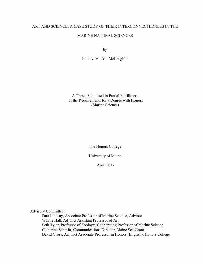
ART AND SCIENCE: A CASE STUDY OF THEIR INTERCONNECTEDNESS IN THE

MARINE NATURAL SCIENCES

by

Julia A. Mackin-McLaughlin

A Thesis Submitted in Partial Fulfillment of the Requirements for a Degree with Honors

(Marine Science)

The Honors College

University of Maine

April 2017

Advisory Committee:

Sara Lindsay, Associate Professor of Marine Science, Advisor Wayne Hall, Adjunct Assistant Professor of Art Seth Tyler, Professor of Zoology, Cooperating Professor of Marine Science Catherine Schmitt, Communications Director, Maine Sea Grant David Gross, Adjunct Associate Professor in Honors (English), Honors College

ABSTRACT

Science and art are interrelated in the form of scientific illustration: the act of observing a

subject and translating the gained knowledge into a visual form. Humans have found

inspiration from the natural world since our beginnings, but the practice of accurately

portraying it arose with the growing interest in natural science in the 15th century. This paper

explores three questions: what is scientific illustration, what is its role in scientific research,

and how has it changed through history? Modern scientific illustration thrives as an effective

method to teach the general public environmental issues. I present a case study using my own

personal artwork to illustrate a literature review of conducted scientific research investigating

the effects of ocean acidification on echinoderms. All echinoderms have calcified structures,

ranging from larval support structures to endoskeletons made of ossicles embedded in the

skin of sea stars, sea cucumbers, and sea urchins, and these structures may be impacted by

acidified conditions. Larval echinoderms are especially at risk. The reviewed literature

suggests that adults exhibit the ability to acclimate to short term acidification, but the long

term impacts are not well understood. To more accurately predict the impact of ocean

acidification on echinoderms, additional research should study long-term exposure and

incorporate impacts on community dynamics as well as individuals.

iii

Dedicated to Carol A. Mackin, to whom I owe my love of art to and who showed me the natural beauty of our

Earth.

iv

ACKNOWLEDGMENTS

I would like to thank everyone on my committee for offering their expert advice and

insightful ideas during the development of this Thesis. I am grateful for having the

opportunity to work with both live and preserved specimens, courtesy of Dr. Seth Tyler, and

use this to improve my own illustrations. I offer a special thanks to Mr. Wayne Hall for his

guidance in creating thoughtful works of art. And finally, my sincere gratitude to my advisor,

Dr. Sara Lindsay, for without her I would never have realized my true passion for scientific

illustration. She has inspired me to follow my heart and be the artist I always dreamed of,

creating works of art for science.

v

TABLE OF CONTENTS

I. Introduction ..........................................................................................................................1

II. Case Study .........................................................................................................................13

Introduction ..........................................................................................................................13

Effects on Survival and Development ..................................................................................16

Effects on Morphology .........................................................................................................20

Effects on Behavior ..............................................................................................................22

Discussion ............................................................................................................................24

Conclusions ..........................................................................................................................26

Figures ....................................................................................................................................27

Artist’s Statement .................................................................................................................50

References ...............................................................................................................................53

Author’s Biography ...............................................................................................................58

vi

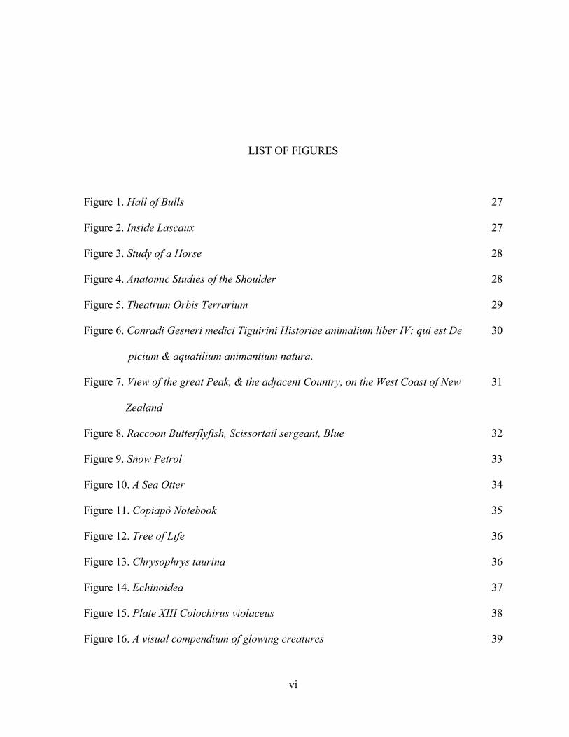
LIST OF FIGURES

Figure 1. Hall of Bulls 27

Figure 2. Inside Lascaux 27

Figure 3. Study of a Horse 28

Figure 4. Anatomic Studies of the Shoulder 28

Figure 5. Theatrum Orbis Terrarium 29

Figure 6. Conradi Gesneri medici Tiguirini Historiae animalium liber IV: qui est De

picium & aquatilium animantium natura.

30

Figure 7. View of the great Peak, & the adjacent Country, on the West Coast of New

Zealand

31

Figure 8. Raccoon Butterflyfish, Scissortail sergeant, Blue 32

Figure 9. Snow Petrol 33

Figure 10. A Sea Otter 34

Figure 11. Copiapò Notebook 35

Figure 12. Tree of Life 36

Figure 13. Chrysophrys taurina 36

Figure 14. Echinoidea 37

Figure 15. Plate XIII Colochirus violaceus 38

Figure 16. A visual compendium of glowing creatures 39

vii

Figure 17. Seafloor of George’s Bank 40

Figure 18. Chemistry of Ocean Acidification 41

Figure 19. Classes of Echinodermata 42

Figure 20. Ophiura Plating 43

Figure 21. Larval Spicule Illumination 44

Figure 22. Adult Biometric Measurement Standards 45

Figure 23. Larval Biometric Measurement Standards 46

Figure 24. Asymmetry and Abnormalities of Larvae 47

Figure 25. Calcite Armor of Ophiura ophiura 48

Figure 26. Asterias rubens consuming Mytilus edulis 49

1

CHAPTER I

INTRODUCTION

Scientific illustration is an expression of visual thinking. It is the act of observing an

object and portraying that which words may fail to convey. The hand of a skilled artist spares

the use of a thousand words. When heart is applied, the natural beauty of a subject emanates.

Depicting the mysteries of the scientific world visually transforms the unknown into the

comprehensible.

During this transformation, the artist must be careful not to lose information through

the subject’s creative presentation. “Whereas a picture can be abstract, ambiguous,

misunderstood, or mistranslated, a picture drawn with skill and accuracy portrays a reality

everyone can relate to” (Magee 2009). The artist needs to be objective: their personal

impression should not influence the product. To achieve this, the artist must integrate correct

colors and proportions, anatomical structures and distinguishing features, into a single

illustration. When applied properly, the subject is not a mechanical blob dribbled onto the

page, but instead breathes life.

This achievement is a valuable tool for science, not as a disposable servant, but as a

keystone to scientific inquiry. Scientists and artists are one of the same. Both are creative in

nature. Both strive for precision. Both feel great passion for their work, fueled by their

insatiable curiosity. Mankind’s endeavor to unlock the world’s secrets is evident since our

beginnings.

Our first documented creative drawing dates back to the Stone Age, when humans

found shelter in mountainside caverns. One example is Lascaux in Southern France. Here,

2

man brought countless creatures to life on the walls, using his bare hands and a mixture of

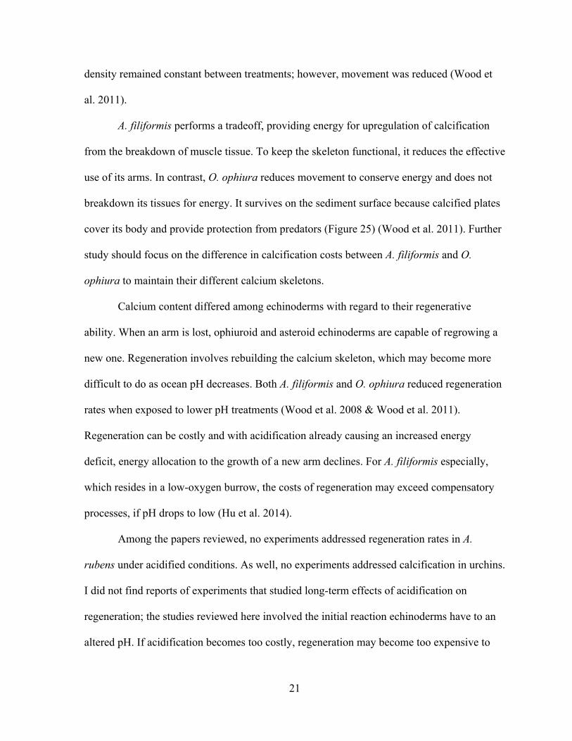
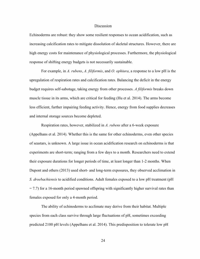
earthly ochre at his side. Figure 1 demonstrates the grandeur of the paintings; a single image

can be upwards of 10 to 15 feet wide (Cosgrove 2014). The paintings depict animals that

surrounded the prehistoric home, such as the mighty oxen and galloping horses of Figure 2.

Some argue that illustrating these animals, which provided a chance at survival, may have

served a spiritual purpose: to assist in religious ceremonies and ensure good luck on future

hunts (Stockstad & Cothren 2013). Prehistoric man found inspiration from the natural world,

incorporating it into his lifestyle as artwork.

This action persisted as human culture developed over time. People continued to

observe their environment, drawing rough representations of their findings. For example, in

the 1st century, a Greek physician, Pendanius Dioscorides, created De Materia Medica: a

five-volume catalog of plants with known medicinal properties. Each plant’s description has

an accompanying illustration for easier identification. During the Han Dynasty, a similar

compilation (the Shennong Becao Jing) documented herbs and medicines used by Chinese to

treat various ailments. In these early times, scientific illustration’s purpose was to identify

flora and fauna that were either medicinally or economically beneficial.

These treatises, however, were uncommon. Up until the 1400s, illustrations were

popular in illuminated manuscripts. Monks incorporated ornate illustrations beside the

written text, but repetitions were rare as the lavish illustrations were all hand drawn.

Repeating them for multiple copies of a book would be tedious and expensive, and the

illustrations would inevitably suffer a decline in precision (Burns 2001). Monasteries that

produced illuminated manuscripts also relied on making their own materials, such as mixing

inks and sizing parchment from dried animal skins (The Metropolitan Museum of Art 2000).

3

The high production cost left commissions generally exclusive to Universities and people of

royalty, adding to the rarity of an already limited practice.

Then, in the 15th century, Johannes Gutenberg invented the printing press. Now,

information spread more rapidly as books became cheaper to reproduce (Principe 2011). An

already established process in China since the 8th century, wood block printing became the

standard for reprinting images in Europe (Suarez 2013). Coinciding with this spread of

knowledge was the growing influence of the Renaissance. It established in Europe a

reverence for knowledge, and as the pursuit of natural science increased in these countries,

by extension, scientific illustration was also refined.

One of the great minds of this era, Leonardo Da Vinci, was an avid illustrator, often

matching written observations with detailed drawings (Da Vinci Science Center 2003). He

used sketches to obtain correct proportions (Figure 3). He also sketched the internal anatomy

of humans (Figure 4). Both of these figures illustrate the developing relationship that exists

between art and science. Da Vinci used both disciplines to improve upon one another. Da

Vinci cites the artist as the perfect person to illustrate laws of nature (Da Vinci Science

Center 2003). He put this argument into practice when he offered illustrations for Luca

Pacioli’s book on mathematics, the De Divina Proportione (Swetz & Katz 2011). He drew

out mathematical and artistic proportions described by Pacioli, who cited their importance in

art and architecture for artists wishing to achieve harmonic forms. His paintings of humans

follow the rules of the golden ratio, a relatively simple geometric construction that appears as

a common metric in organismal design (Meisner 2014).

By incorporating mathematical formulas such as the golden ration, Da Vinci brought

greater realism to his scientific subjects. He also is an example of the broader application of

4

scientific illustration beyond just botanicals. Many artists during the Renaissance found

inspiration to accurately portray not just plants but animals, humans, and architecture.

Following the Renaissance, growing interest in new fields coincided with the Scientific

Revolution, during which natural science developed as its own discipline in European

culture. The accompanying growth in scientific rigor towards the natural world influenced

scientists to incorporate greater authenticity in the assisting illustrations produced. In this

way, illustrations became more efficient at conveying notes and observations or clarifying

ideas or hypotheses.

Although scientific and natural history illustrations increased in realism, such visuals

generally focused on terrestrial environments or the heavens, leaving out one massive part of

the world: the oceans. Marine natural science lagged behind, with the significant

advancements made only in regions along the coast. The difficulty in depicting accurate

illustrations was a result of Europeans lacking the equipment enabling scientific exploration

of marine life. Poor accessibility made it difficult for natural scientists to investigate beyond

coastal environments, and artists usually relied on the descriptions brought back by sailors.

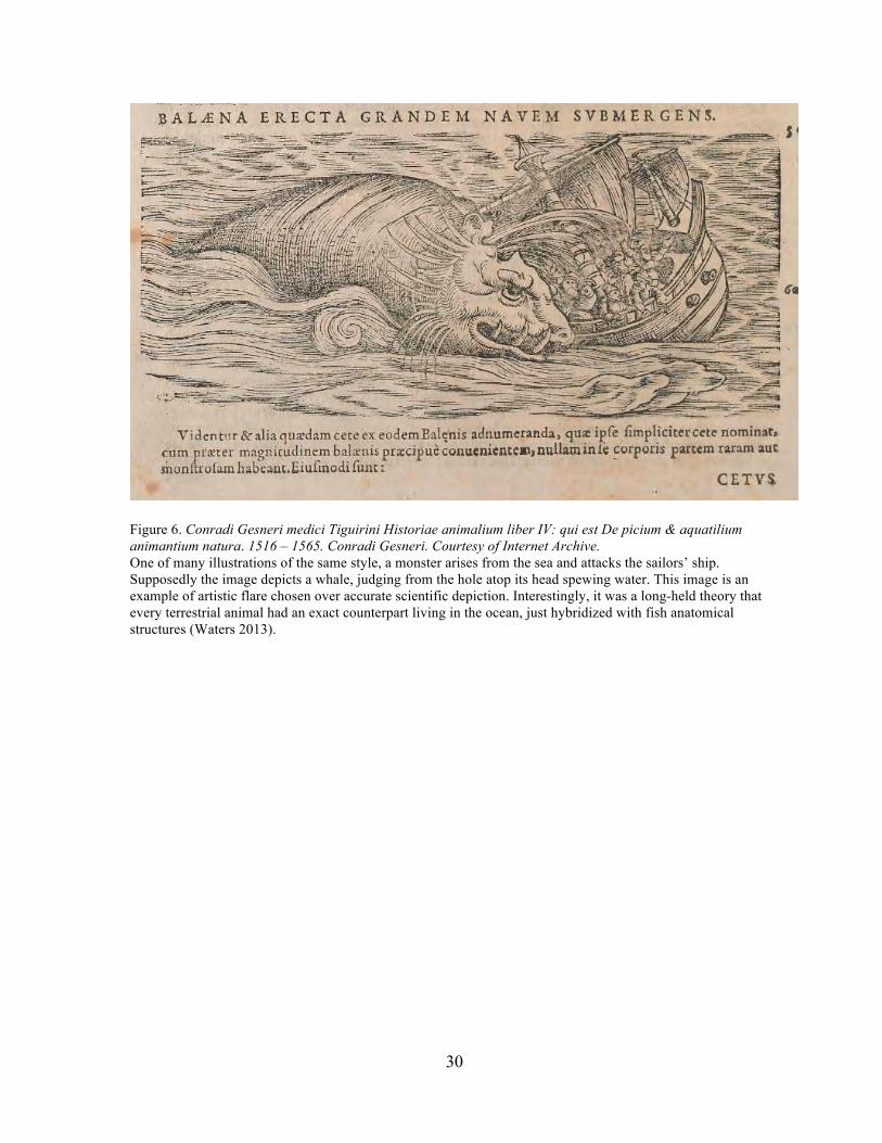
The artist’s creativity filled in the knowledge gaps. Figure 5 presents a section of the

Theatrum Orbis Terrarium, the first modern world atlas, published in 1570 (Waters 2013).

The animal depicted is a combination of an artist’s educated guess and the biblical story of

Jonah. In zoological treatises, marine fauna showed greater stylization of subject matter than

the terrestrial counterparts (Figure 6). Such stylized illustrations with their absences of

accuracy proliferated up until the 18th century.

Then, European governments began sponsoring voyages of conquest, and explorers,

military men, and scientists embarked on journeys across the vast oceans. The draw of exotic

5

worlds with new discoveries enticed scientists to explore. Naturalists and artists alike

accompanied the greatest explorers, their prowess an appreciated skill never left behind

because through their work, Europeans had the opportunity to visualize what the rest of the

world looked like. The brilliant minds unable to join these expeditions could still compare

and contrast the animals, plants, and minerals from around the world by using the

illustrations. When artists ensured their work was accurate, illustrations became a bridge,

expressing information of a subject to a viewer. Instead of relying on their own imaginations,

Europeans now had an informed understanding of the diversity in the world around them.

A pioneer of exploration was the British Lieutenant Captain James Cook, who in

1768 set sail on his first voyage aboard the H.M.S. Endeavor. He explored the South Pacific,

discovering the great lands of Australia and New Zealand for the British before returning to

London in 1771 (Cook & Price 1971). Accompanying Captain Cook was the resident artist,

Sydney Parkinson. As the Endeavor traversed the Pacific Ocean, Parkinson illustrated the

indigenous people and expansive landscapes encountered, as well as the specimens collected

by his employer, the influential British naturalist Joseph Banks (Natural History Museum

2010). Parkinson would sketch out what he saw, incorporating labels for key colors. This

code was reference for when he finalized his work at home in London.

Unfortunately, the young man never returned home, as he died of dysentery in 1770

(State Library of New South Wales 2016). His sketches, however, did make it back and his

foresight to include color codes meant other artists could finish his work. Figure 7 depicts

one example of the many prints rendered from his sketches, found in A Journal of a voyage

to the South Seas.

6

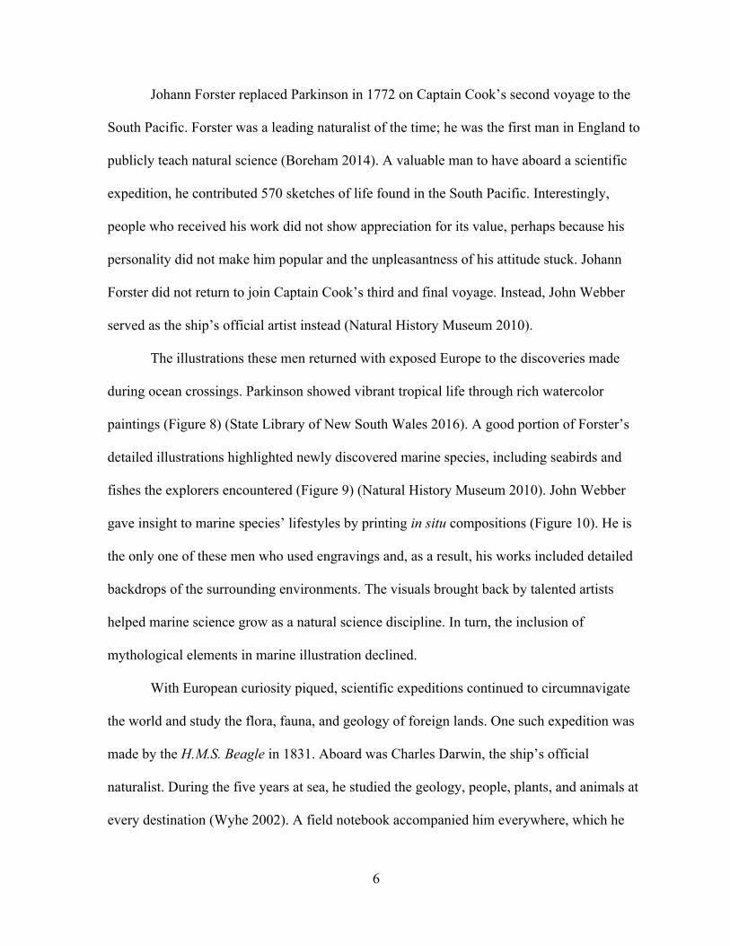
Johann Forster replaced Parkinson in 1772 on Captain Cook’s second voyage to the

South Pacific. Forster was a leading naturalist of the time; he was the first man in England to

publicly teach natural science (Boreham 2014). A valuable man to have aboard a scientific

expedition, he contributed 570 sketches of life found in the South Pacific. Interestingly,

people who received his work did not show appreciation for its value, perhaps because his

personality did not make him popular and the unpleasantness of his attitude stuck. Johann

Forster did not return to join Captain Cook’s third and final voyage. Instead, John Webber

served as the ship’s official artist instead (Natural History Museum 2010).

The illustrations these men returned with exposed Europe to the discoveries made

during ocean crossings. Parkinson showed vibrant tropical life through rich watercolor

paintings (Figure 8) (State Library of New South Wales 2016). A good portion of Forster’s

detailed illustrations highlighted newly discovered marine species, including seabirds and

fishes the explorers encountered (Figure 9) (Natural History Museum 2010). John Webber

gave insight to marine species’ lifestyles by printing in situ compositions (Figure 10). He is

the only one of these men who used engravings and, as a result, his works included detailed

backdrops of the surrounding environments. The visuals brought back by talented artists

helped marine science grow as a natural science discipline. In turn, the inclusion of

mythological elements in marine illustration declined.

With European curiosity piqued, scientific expeditions continued to circumnavigate

the world and study the flora, fauna, and geology of foreign lands. One such expedition was

made by the H.M.S. Beagle in 1831. Aboard was Charles Darwin, the ship’s official

naturalist. During the five years at sea, he studied the geology, people, plants, and animals at

every destination (Wyhe 2002). A field notebook accompanied him everywhere, which he

7

filled with scribbly notes and cryptic doodles (Figure 11). Darwin’s many notebooks tell the

story of his intellectual development that led to his developing the theory of evolution

through natural selection (Wyhe 2002).

Darwin’s observations led him to realize the intertwined ancestry of life: that all

species share a common ancestor and the diversity of modern life arose from the differential

success of heritable traits in survival and reproduction. He included in his book, On the

Origin of Species, an illustrated figure to clarify his theory (Figure 12). This figure, the Tree

of Life, turns the complicated writing into a single, easily-understood visual that supports and

translates his groundbreaking and controversial idea.

Darwin did not produce all the illustrations included in his publications. He, like

many scientists, relied on the skills of artists hired from a guild. These services immortalized

the specimens he collected during his travels. Titled The Zoology of the Voyage of H.M.S.

Beagle, the collaboration resulted in five volumes filled with images of fossils, mammals,

birds, fishes, and reptiles found through the Beagle’s expedition (Figure 13). Volume IV

focused on the fishes and was one of the most neglected of the five volumes. While Darwin

obviously had some interest in fish, as indicated by the scattered observations in his notes

and publications, it was not a major interest to him. He never actually authored a book or

paper devoted solely to ichthyology. He only edited the volume describing fishes

encountered. The actual author was the Reverend Leonard Jenyns.

Most naturalists of this time period, like Darwin, were not specifically searching for

fishes and marine mammals. Their interests were general; whatever they encountered they

would observe, describe, and illustrate, including marine fauna. However, technology

continued to limit the depth of research on marine natural science. It was either too expensive

8

or not yet possible. In the 18th century, while explorers circumnavigated the globe, the deep

sea was still unreachable. Scientists believed it was void of life, an azoic zone. In 1843,

Edwards Forbes claimed life could not exist below 300 fathoms, roughly 550 meters, below

the ocean surface (NOAA 2008). No one imagined anything survived in the endless darkness

and crushing pressures found at these depths.

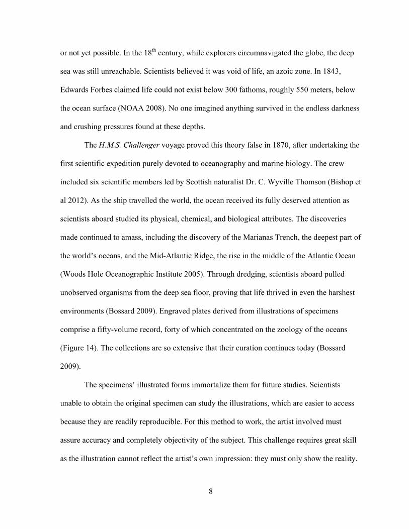
The H.M.S. Challenger voyage proved this theory false in 1870, after undertaking the

first scientific expedition purely devoted to oceanography and marine biology. The crew

included six scientific members led by Scottish naturalist Dr. C. Wyville Thomson (Bishop et

al 2012). As the ship travelled the world, the ocean received its fully deserved attention as

scientists aboard studied its physical, chemical, and biological attributes. The discoveries

made continued to amass, including the discovery of the Marianas Trench, the deepest part of

the world’s oceans, and the Mid-Atlantic Ridge, the rise in the middle of the Atlantic Ocean

(Woods Hole Oceanographic Institute 2005). Through dredging, scientists aboard pulled

unobserved organisms from the deep sea floor, proving that life thrived in even the harshest

environments (Bossard 2009). Engraved plates derived from illustrations of specimens

comprise a fifty-volume record, forty of which concentrated on the zoology of the oceans

(Figure 14). The collections are so extensive that their curation continues today (Bossard

2009).

The specimens’ illustrated forms immortalize them for future studies. Scientists

unable to obtain the original specimen can study the illustrations, which are easier to access

because they are readily reproducible. For this method to work, the artist involved must

assure accuracy and completely objectivity of the subject. This challenge requires great skill

as the illustration cannot reflect the artist’s own impression: they must only show the reality.

9

Artists are still capable of incorporating their own flare within a piece without

misrepresenting of the subject. Ernst Haeckel, a German naturalist of the 19th century, found

this specific balance between artistic passion and scientific discipline by creating works of art

to explain and support his theories. Before he became a scientific illustrator, he dedicated his

life to watercolor landscape paintings (Lebrun 2004). He never found fulfillment in just

painting; he realized his true passion when microscopic organisms piqued his interest

(Breidbach et al 2009). His work is distinguished for its quality; the many specimens he

illustrated are elaborately detailed. Beyond drawings of phytoplankton, Haeckel illustrated a

generous number of various marine animals (Figure 15). He was a prominent naturalist,

whose ideas were influential in science at the time. Haeckel offered support for Darwin’s

theory of evolution through illustration. His voluminous publications peppered with detailed

visuals taught more people about the new idea than did Darwin’s own writings (Richards

2009). Interestingly, while Haeckel was vehemently defending evolution with his drawings, a

new method was developing that would offer a revolution in visual arts: photography.

Suddenly, the ability to grasp pure objectivity appeared.

Photography’s popularity grew through the 1800s and was well established in every

industrialized nation by the turn of the century (Osterman 2013). At first, people were

skeptical of its seriousness as an art form. But it takes artistic skill and chemical knowledge

to be a successful photographer, as anyone who has dabbled in serious photography will

agree. A good final product requires the photographer to use the same techniques any artist

using traditional media would enlist, such as setting up an interesting composition.

Photography is a tool with its own drawbacks that illustration can overcome. While

photography depends on sufficient light to illuminate a subject, and is limited to the subject

10

at hand, there is greater control in what is included in an illustration. A photograph is less

selective. An artist can take broken pieces and rebuild the specimen, like reconstructing an

extinct species through a fossilized skeleton. An artist has the ability to show the viewer the

unobservable, from a molecular makeup to the expanses of space.

Which approach to visualization is appropriate becomes a question of what the

scientist is asking. Photography is just as viable a tool for illustration as traditional media, but

it is independent through its unique style of capturing an image of a subject at a single

moment in time. The artist should consider the advantages and disadvantages of both styles.

For example, taking a photo of a protein or DNA gel is more practical then drawing it out. As

well, a photo can capture in situ information of an organism in its natural habitat. However,

illustration through traditional media can emphasize areas or structures of interest and

illustrate processes, such as the complex internal physiology of the human body. Trying to

photograph a specific portion is difficult as the image becomes overwhelmed with

unnecessary detail.

Today, combining both photographic and traditional methods will yield the best

results for scientific illustrators. Each technique can compensate for the other’s

shortcomings. But, as photography became more common and accessible during the 20th

century, it supplanted more traditional methods of illustration. Depicting science shifted

towards a more aesthetically sterile approach (Popova 2012). But illustrators continued to

employ traditional forms, including watercolors, oil paints, inks and graphite. Now, as

technology continues to advance, illustrators have adapted to include more modern

applications.

11

Programs such as Adobe Photoshop give artists more control by enabling them to

retouch photographs. For example, blurring the backdrop can make the subject more

apparent, where otherwise it could be overwhelmed. In other programs such as Adobe

Illustrator, an artist can begin with a blank digital canvas and create an illustration from

scratch. The kinds of programs useable are endless, some even enabling the use of three-

dimensional renderings.

Eleanor Lutz is an example of someone who utilizes computer programs to better

supplement a body of scientific illustration. For example, she illustrated a phylogenetic tree

that organizes the occurrence of organismal bioluminescence throughout the different

kingdoms (Figure 16). While the illustration is not strictly limited to marine taxa, it serves as

an example of how scientific illustration communicates a message through visualization.

With this illustration, Lutz conveys the diversity and evolutionary history of bioluminescent

organisms as well as their morphology and the color of their bioluminescence. Data

visualization in the form of infographics is a modern version of scientific illustration that

uses both words and images to present information quickly to a general audience (Bayliss–

Brown 2014). The images aid cognitive functions and so their incorporation makes the

content not only easier to understand, but also easier to remember. For marine science, I

believe this technique can help teach people about how humans have caused change in the

world’s oceans.

Lutz is also an example of how scientific artists are curious in nature. She tried out

scientific illustration during a gap year after graduating college (Lutz 2014). Many artists

dedicate their lives to scientific illustration because they are interested in learning. For

example, when NOAA sponsored the Deep East Voyage of Discovery expedition to study the

12

ocean floor in 2001, two scientific illustrators joined the crew. They mapped out what

George’s Bank looked like by watching videos recorded by the deep-sea submersible Alvin

(Figure 17). They also sketched specimens brought up by Alvin to the surface. Bringing a

specimen from the seafloor usually involves crushing or breaking it, but the onboard artist

recreated its original form (NOAA 2010). He did so using traditional media as well; in this

case paints. Many artists embrace both traditional and digital methods. Even with the advent

of digital art, traditional media still remains prolific in the scientific illustration community.

The importance of illustration is not a derivative of the chosen method, but of artist’s

illustration achieving its goal.

Scientists appreciate this benefit to their work. Scientific illustrators combine their

curiosity and creativity with their design prowess to become the “eyes” of scientists. The

artists aboard were noticeably curious of NOAA’s work during the expedition, because they

share interest in what scientists are discovering. Illustrators combine skill, curiosity, and

creativity to create works of art that influence and elaborate on science’s greatest endeavors.

In this thesis, I share with readers my own case study on the interrelationship between

art and science. In addition to surveying how scientific illustration (especially of marine

subjects) has progressed through time, I have conducted a literature review on how the

current phenomenon of ocean acidification is affecting echinoderms of the North Atlantic. To

build experience translating this science in to art, I created several scientific illustrations that

serve to elaborate on concepts and hypotheses discussed. The original artworks were

displayed in a show accompanying my thesis defense and digital images of them are included

in this thesis so that the reader might gain an appreciation of the bond between science and

art.

13

CHAPTER II

CASE STUDY: OCEAN ACIDIFCATION’S IMPACT ON ECHINODERMS

Introduction

Earth’s oceans are undergoing a momentous change as a result of increased

atmospheric CO2 from anthropogenic sources. Processes such as fossil fuel burning and

cement production have contributed to the total atmospheric CO2 (CO2atm) partial pressure

increasing from 280 ppm to 400 ppm. This represents a 40% increase in the earth’s total

CO2atm concentration (Doney et al. 2009). The ocean is a sink: already it has absorbed one

third of the released CO2 from the atmosphere (Royal Society 2005). As aqueous CO2

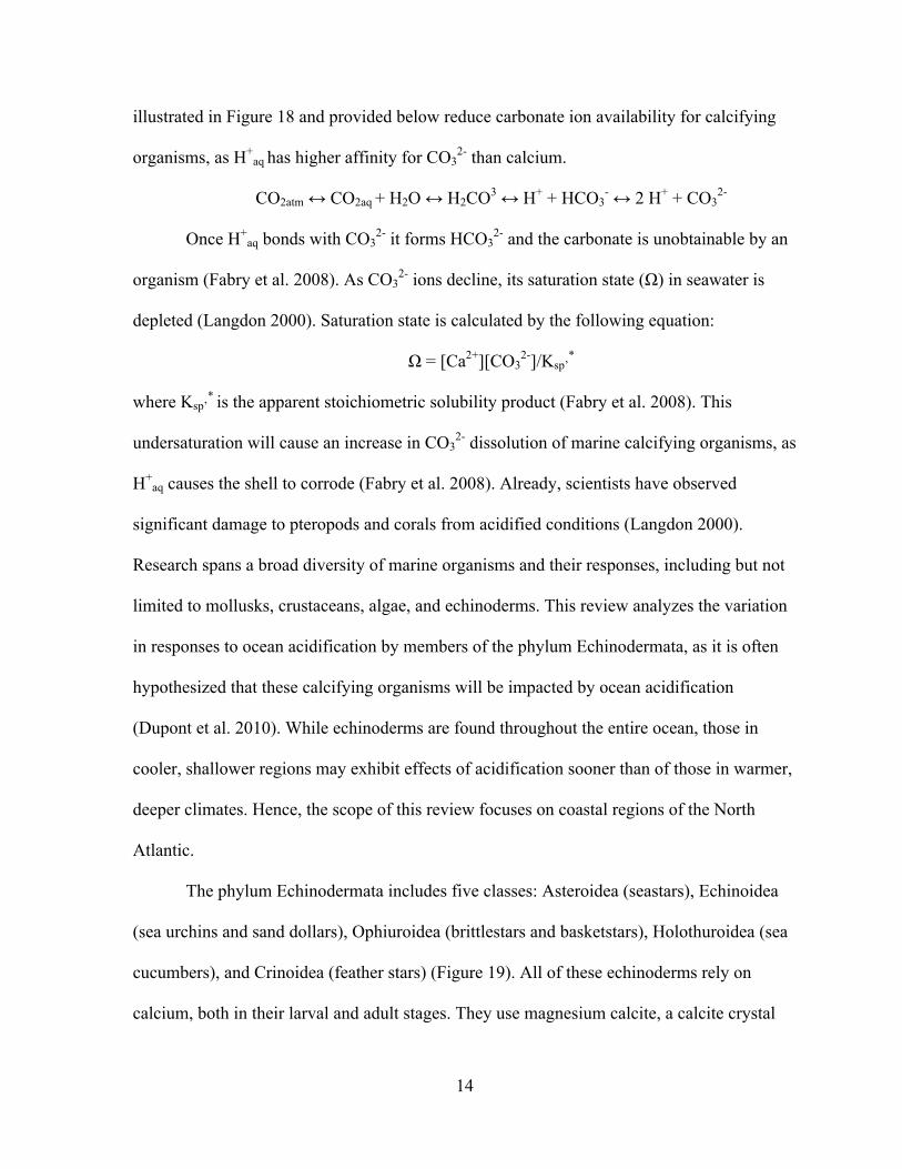
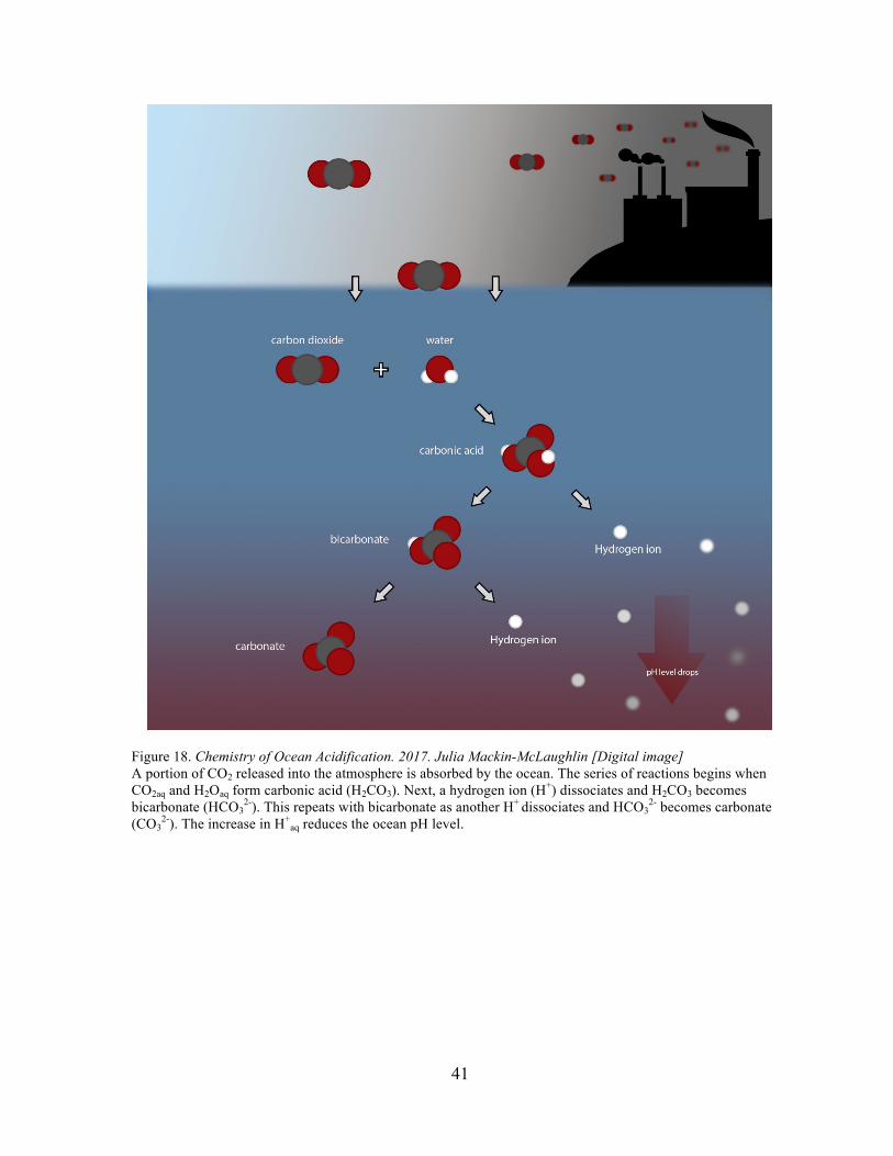
(CO2aq) interacts with H2O, it goes through a series of reactions releasing H+aq as an end

product (Figure 18) (Orr et al. 2005). More CO2atm absorbed into the ocean yields greater

H+aq concentrations, causing ocean pH levels to decline. This phenomenon is referred to as

ocean acidification.

The surface ocean pH has decreased by a 0.1 unit since the pre-industrial era (Doney

et al. 2009), and the current average ocean pH is 8.1, although local pH conditions can vary.

The measurement of pH uses a logarithmic scale, meaning this 0.11 unit drop represents a

30% increase in the total H+aq concentration in the world’s oceans. Scientists predict the

decline will continue and that there will be a 0.4 unit drop in surface ocean pH by 2100

(Dupont et al. 2010). This change is occurring rapidly on the geological timescale and the

increase in H+aq concentrations poses a threat to marine biota.

Many take up carbonate (CO32-) from surrounding seawater and combine it with

calcium (Ca2+) to build shells and skeletal structures. The reactions of ocean acidification

14

illustrated in Figure 18 and provided below reduce carbonate ion availability for calcifying

organisms, as H+aq has higher affinity for CO3

2- than calcium.

CO2atm ↔ CO2aq + H2O ↔ H2CO3 ↔ H+ + HCO3- ↔ 2 H+ + CO3

2-

Once H+aq bonds with CO3

2- it forms HCO32- and the carbonate is unobtainable by an

organism (Fabry et al. 2008). As CO32- ions decline, its saturation state (Ω) in seawater is

depleted (Langdon 2000). Saturation state is calculated by the following equation:

Ω = [Ca2+][CO32-]/Ksp’

*

where Ksp’* is the apparent stoichiometric solubility product (Fabry et al. 2008). This

undersaturation will cause an increase in CO32- dissolution of marine calcifying organisms, as

H+aq causes the shell to corrode (Fabry et al. 2008). Already, scientists have observed

significant damage to pteropods and corals from acidified conditions (Langdon 2000).

Research spans a broad diversity of marine organisms and their responses, including but not

limited to mollusks, crustaceans, algae, and echinoderms. This review analyzes the variation

in responses to ocean acidification by members of the phylum Echinodermata, as it is often

hypothesized that these calcifying organisms will be impacted by ocean acidification

(Dupont et al. 2010). While echinoderms are found throughout the entire ocean, those in

cooler, shallower regions may exhibit effects of acidification sooner than of those in warmer,

deeper climates. Hence, the scope of this review focuses on coastal regions of the North

Atlantic.

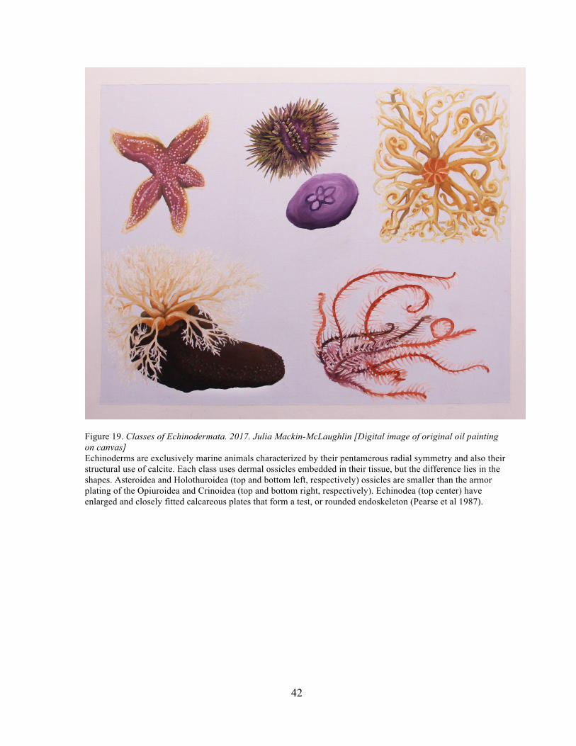
The phylum Echinodermata includes five classes: Asteroidea (seastars), Echinoidea

(sea urchins and sand dollars), Ophiuroidea (brittlestars and basketstars), Holothuroidea (sea

cucumbers), and Crinoidea (feather stars) (Figure 19). All of these echinoderms rely on

calcium, both in their larval and adult stages. They use magnesium calcite, a calcite crystal

15

precursor, to build multiple calcite structures (Dupont et al. 2010). The adults of every class

have an endoskeleton embedded in the body tissue, covered by an epidermis. The skeletal

frame is achieved by joining calcareous plates, or ossicles, together with connective tissue

(Pearse et al. 1987). It is class dependent on how prominent the calcium structures are in the

animal. For example, ophiuroid species have substantial calcium plating, compared with the

finer ossicles of asteroids (Figure 20). In contrast, echinoderm larvae are a distinctly different

life stage, temporarily occupying the pelagic zone, unlike their benthic adult counterparts

(Dupont et al. 2010). Larvae of the Echinoidea and Ophiuroidea classes have skeletal

calcareous rods within their arms (Pearse et al 1987). The arms provide support and assist in

feeding, as well influencing body shape, larval orientation, and swimming efficiency (Dupont

et al. 2008; Stumpp et al. 2012) (Figure 21).These skeletal structures are largely absent in

larvae of the remaining three echinoderm classes.

Ocean acidification could lead to drastic shifts in community structures and trophic

cascades by affecting the integrity of an echinoderm’s skeletal structure (Doney et al. 2009).

Echinoderms are keystone species in benthic habitats, meaning they play a unique or critical

ecological role that numerous other species depend on. Their roles include both predator and

prey, and they often act as ecosystem engineers that significantly influence the habitat they

reside in. For example, Amphiura filiformis is an infaunal brittlestar that acts as a bioturbator

by constructing its burrow in the sediment. It uses its arms to circulate oxygen into its burrow

and thus provides localized oxygen to deeper, oxygen-poor sediments that would otherwise

not support oxygenic bacteria and microscopic invertebrates (Wood et al. 2009).

The purpose of this chapter is to review effects of ocean acidification on

echinoderms, specifically those found in the North Atlantic and illustrate some aspects of that

16

research with original artwork. I focus on the survival, morphology, and behavior of various

species of Echinoidea, Asteroidea, and Ophiuroidea because there was little published

research involving the effects of ocean acidification on Crinoidea and Holothuroidea. This

review will synthesize published research on the effects of ocean acidification and use it to

predict responses of echinoderms in general. This review also addresses gaps in the available

knowledge and gives advice for future experiments.

Effects on Survival and Development

Ocean acidification will most likely not be lethal to adult echinoderms. In the reports

reviewed, mortality of adults during exposure to seawater with pH <8.1 (the current

worldwide average and experimental control) was rare. In the seven studies reviewed, only

three deaths of adult green sea urchins, Strongylocentrotus droebachiensis, occurred in

acidified conditions (pH = 7.10) (Stumpp et al. 2012). Adults show the potential to survive

short term exposure to acidified waters, but stress of acidification causes an organism’s

energy budget to shift.

In reduced pH conditions, maintaining acid-base balance and calcification rates may

require greater expenditure of energy. How echinoderms mitigate this negative effect is

species-specific. Some alter respiration rates. For example, when exposed to an acidified

treatment, the brittlestar Ophiura ophiura increased its oxygen consumption (Wood et al.

2010). Alternatively, another species of the same Ophiuroidea class, Amphiura filiformis,

decreased oxygen consumption (Hu et al. 2014). The difference in habitat of both species

may be the cause of the difference in response. O. ophiura is epifaunal and lives above the

sediment while A. filiformis is infaunal and creates a burrow to live and feed in.

17

When exposed to an acidified condition of pH = 7.0, A. filiformis retracts its arms

from the water column and into its burrow (Hu et al. 2014). As a result, it does not replenish

oxygen supplies to its burrow, and therefore cannot increase oxygen consumption. Being

above the sediment, O. ophiura has a more regular supply of oxygen available, enabling it to

increase oxygen consumption (Wood et al. 2009).

Adults of S. droebachiensis exposed to reduced pH altered growth rates instead of

respiration rates (Stumpp et al. 2012). Test diameter and gut and gonadal mass declined in S.

droebachiensis adults exposed to a low pH of 7.10, compared to a pH of 7.8 (Figure 22)

(Stumpp et al. 2012). Reducing somatic and gonadal tissue conserves energy for

maintenance.

Some echinoderms exhibit the ability to acclimate to acidified conditions. The

common sea star, Asterias rubens, initially upregulated respiration rates when it was exposed

to a low (pH = 7.4) and an intermediate (pH = 7.7) pH treatment. This increase occurred after

a 27-day exposure (Collard et al. 2013). In a separate experiment, A. rubens showed no

difference in respiration rates between control (pH = 7.86), intermediate (pH = 7.72), and

low (pH = 7.24) treatments after a six-week exposure (Appelhans et al. 2014).

The difference in pH treatments used may have influenced the results. Collard &

colleagues (2013) used a control pH treatment of 8.0. Appelhans and others (2014) used a

control treatment of 7.86, which is closer to the intermediate pH treatment of the former

experiment than to their own control pH. Collard and others (2013) found no difference in

respiration rates between the low and intermediate pH treatments; the only significant

difference after a 27-day exposure duration was that the control treatment did not cause A.

rubens to upregulate respiration rates. Therefore, it is possible that Appelhans and others

18

(2014) found no difference in respiration rates after six weeks because the control pH was

too low to accurately represent a difference in current conditions with future acidified

conditions.

Only a few experiments have investigated the potential of echinoderms to acclimate

to low pH for a long time period. Dupont and others (2013) studied the ability of S.

droebachiensis to acclimate by exposing females to acidic conditions for either 4 months or

16 months. Females exposed for 16 months showed no significant difference in fecundity,

regardless of pH treatment. Females exposed to a low pH treatment for only 4 months saw a

450% decrease in fertilization success. Mortality rates of larvae differed, depending on the

exposure of the mother. Females exposed to the low pH treatment for 4-months produced

young that suffered an increase in mortality, but there was no significant difference in

mortality of young between treatments of those females exposed for 16-months.

Acclimation still requires shifts in energy allocation from other physiological

processes, such as growth. For example, exposure to a low pH treatment (pH = 7.9) caused a

3-fold decline in arm length and significantly lower quantities of wet and dry masses in A.

rubens (Figure 22) (Keppel et al. 2014 & Appelhans et al. 2014). Unfortunately, the long-

term studies did not include measuring respiration rates.

If echinoderms fail to acclimate to acidified conditions, adult fecundity and larvae

seem to be the most at risk. In the studies reviewed, researchers observed little adult

mortality, but demonstrated increases in abnormalities of eggs and larvae and in larval

mortality. For example, Bögner and others (2014) visually assessed a fertilized egg’s health

by analyzing the quality of its fertilization envelope. Lower pH treatments (pH = 7.8, 7.71,

7.39) yielded a higher proportion of unhealthy eggs.

19

Even if the smaller proportion of eggs are successfully fertilized, larval development

is more difficult in an acidified environment. Dorey and others (2013) and Dupont and others

(2008) measured growth rates and developmental health of larvae of S. droebachiensis and

Ophiothrix fragilis by measuring the biometric standards illustrated in Figure 23. Both

studies found larval mortality rates increased in lower pH treatments. Those larvae that

survived had smaller body lengths and developed slower. Dupont and others (2008)

measured the occurrence of asymmetrical and abnormal O. fragilis larvae (Figure 24). No

larvae were asymmetrical or abnormal in the control pH treatment (pH = 8.1). These

detrimental effects occured when pH treatments are low, such as 7.7 or 7.9.

Acidification may affect development by changing the larvae’s acid-base status and

altering the larval spicules. It may also affect feeding capability by reducing arm length and

decreasing energy acquisition, contributing to their slower development (Dorey et al. 2013).

Slower and unhealthy development may lead to declines in echinoderm populations.

Experiments finding reduced growth and increased respiration had short-term exposure

times.

There is a need for longer duration experiments, like that of Dupont and others (2013)

on S. droebachiensis. A 16-month exposure time yielded higher larval survival rates than a 4-

month exposure duration. Plasticity of echinoderm larval responses to acidification may be at

play. For example, echinoderms in coastal regions already often deal with pH levels that are

equal to the low or intermediate pH treatments used in these perturbation experiments as a

result of oceanographic processes such as upwelling. Some species may have pre-adaptations

to these low pH levels, preparing them to survive current trends of acidification.

20

Effects on Morphology

Calcification is the primary physiological process threatened by acidification. As

oceans continue to acidify, building skeletons will become more difficult with increased

pressure of increased dissolution rates, causing degradation in the echinoderms. Wood and

others (2008) supported this claim by removing the arms of A. filiformis and exposing

different samples to different pH treatments. Arms exposed to lower pH treatments had lower

calcium content.

Echinoderms replenish lost calcium through calcification. When Wood and others

(2008) exposed adult A. filiformis to a set of reduced pH treatments (pH = 7.7, 7.3, 6.8),

compared to a control of pH = 8.0, there was a linear increase in calcification rates with the

reduction. Calcium content of arms between treatments did not differ significantly, as A.

filiformis replenished the calcite lost through dissolution. The same is observed in O. ophiura

exposed to the same control and low pH levels: net calcification was not significantly

different between treatments (Wood et al. 2010). O. ophiura upregulated its calcification rate

as more calcium dissolved and achieved a net balance. A. rubens also upregulated its

calcification when exposed to a low pH, so much so that a greater ratio of calcified to soft

tissue was observed (Keppel et al. 2014).

Evidence suggests that echinoderms show resilience against an acidic environment,

increasing calcification rates to compensate for reduced availability of carbonate in the

seawater. Similar to upregulation of respiration, echinoderms balance out the energy budget

and accommodate for the energy deficit. A. filiformis does so through muscle wastage, which

occurred when exposed to a low pH treatment (Wood et al. 2008). In O. ophiura, muscle

21

density remained constant between treatments; however, movement was reduced (Wood et

al. 2011).

A. filiformis performs a tradeoff, providing energy for upregulation of calcification

from the breakdown of muscle tissue. To keep the skeleton functional, it reduces the effective

use of its arms. In contrast, O. ophiura reduces movement to conserve energy and does not

breakdown its tissues for energy. It survives on the sediment surface because calcified plates

cover its body and provide protection from predators (Figure 25) (Wood et al. 2011). Further

study should focus on the difference in calcification costs between A. filiformis and O.

ophiura to maintain their different calcium skeletons.

Calcium content differed among echinoderms with regard to their regenerative

ability. When an arm is lost, ophiuroid and asteroid echinoderms are capable of regrowing a

new one. Regeneration involves rebuilding the calcium skeleton, which may become more

difficult to do as ocean pH decreases. Both A. filiformis and O. ophiura reduced regeneration

rates when exposed to lower pH treatments (Wood et al. 2008 & Wood et al. 2011).

Regeneration can be costly and with acidification already causing an increased energy

deficit, energy allocation to the growth of a new arm declines. For A. filiformis especially,

which resides in a low-oxygen burrow, the costs of regeneration may exceed compensatory

processes, if pH drops to low (Hu et al. 2014).

Among the papers reviewed, no experiments addressed regeneration rates in A.

rubens under acidified conditions. As well, no experiments addressed calcification in urchins.

I did not find reports of experiments that studied long-term effects of acidification on

regeneration; the studies reviewed here involved the initial reaction echinoderms have to an

altered pH. If acidification becomes too costly, regeneration may become too expensive to

22

perform. This is a real threat given that injury and regeneration are common occurences

among asteroids and ophiurouds (ranging from 10% to 99% of individuals depending upon

species) (Lindsay 2010). Arms are critical for feeding: A. filiformis uses them for suspension

feeding and A. rubens utilizes the calcite ossicles of its skeletal system in their arms to pry

mussel shells apart (Hu et al. 2014 & Appelhans et al. 2014).

Effects on Behavior

Acidification is likely to drive changes in echinoderm behavior. Echinoderms are

motile animals and pH changes influence their mobility. For example, seastars and

brittlestars will right themselves if turned upside down. This righting response remained

unaffected by pH changes in A. rubens but changed in O. ophiura (Appelhans et al. 2009)

(Wood et al. 201). O. ophiura was faster to right itself in low pH treatments (pH = 7.3), but

only when the water temperature was lowered 10.5ºC (Wood et al. 2010). There was no

significant difference in righting response when the temperature was 15ºC.

The greatest change in behavior echinoderms exhibited in response to acidification

was in feeding. Echinoderm feeding rates declined as pH levels dropped. Stumpp and others

(2012) dissected adult S. droebachiensis after exposing them to low pH treatments. They

found that 71% of animals exposed to a lowest pH had empty guts, but this did not occur in

any urchins in the intermediate pH treatments (pH = 7.51). Only in S. droebachiensis larvae

did a decrease in pH cause an increase in ingestion rates (Dorey et al. 2013).

Body tissue mass may decline as less food is ingested, yielding less energy. Across

most studies on A. rubens, biomass declined with a drop in pH (Appelhans et al. 2014 &

Keppel et al. 2014). Ingestion rates of M. edulis declined as A. rubens reduced its foraging

23

behavior in low pH treatments (pH = 7.24) (Appelhans et al. 2014). Physiological issues,

such as impaired sensory processes, could have inhibited the ability to forage.

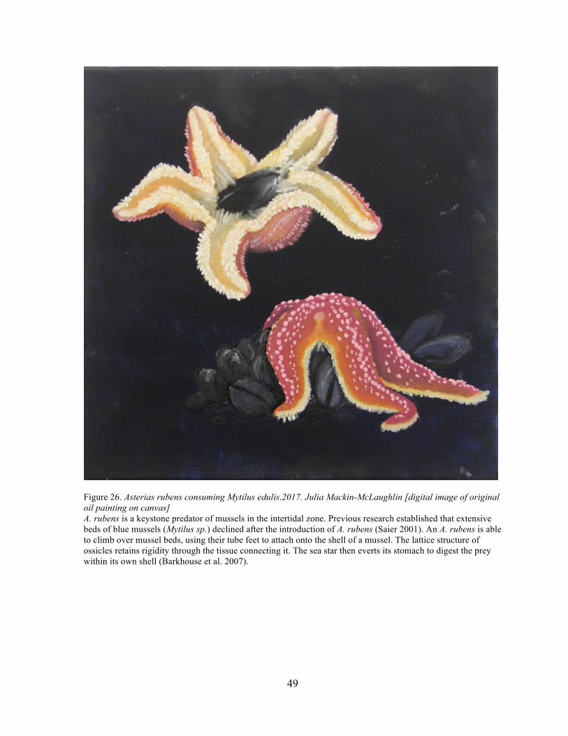
Acidification could affect the technique used by asteroids to feed. Seastars have small

ossicles embedded in their dermis and thus their endoskeletons are less pronounced than the

tests of the Echinoids (Dupont et al. 2010). Nonetheless, these calcified ossicles and the

muscles that link them represent a pivotal feature that enables seastars to pry open mussels

found in the intertidal (Figure 26). Because seastars are often keystone predators that keep

intertidal and subtidal populations of mussels in check, impacts on feeding behavior may

have indirect impacts on the community.

A reduction in ingestion rates may be the result of avoidance of stressors as well. A.

filiformis reduced the time arms were above the sediment surface filter-feeding as the pH

decreased. A 56% decrease in activity was observed between control (pH = 8.1) and

intermediate (pH = 7.3) pH treatments and a 73% decrease was observed between control

and low pH treatments (pH = 7.0) (Hu et al. 2014). Because A. filiformis activity oxygenates

the sediment and influences sediment biogeochemistry, reduced irrigation could impact

fluxes between the sediment and water column and the microbial and microbenthic

community surrounding A. filiformis burrows.

As these examples illustrate, with such reductions in feeding activity by echinoderms,

shifts in community structures may arise as an indirect consequence of ocean acidification.

Most experiments investigating the impacts of ocean acidification use perturbation of a single

species outside of its environment. It is difficult to predict future conditions if research does

not extend to trophic cascades and the roles echinoderms have within them.

24

Discussion

Echinoderms are robust: they show some resilient responses to ocean acidification, such as

increasing calcification rates to mitigate dissolution of skeletal structures. However, there are

high energy costs for maintenance of physiological processes. Furthermore, the physiological

response of shifting energy budgets is not necessarily sustainable.

For example, in A. rubens, A. filiformis, and O. ophiura, a response to a low pH is the

upregulation of respiration rates and calcification rates. Balancing the deficit in the energy

budget requires self-sabotage, taking energy from other processes. A filiformis breaks down

muscle tissue in its arms, which are critical for feeding (Hu et al. 2014). The arms become

less efficient, further impairing feeding activity. Hence, energy from food supplies decreases

and internal storage sources become depleted.

Respiration rates, however, stabilized in A. rubens after a 6-week exposure

(Appelhans et al. 2014). Whether this is the same for other echinoderms, even other species

of seastars, is unknown. A large issue in ocean acidification research on echinoderms is that

experiments are short-term; ranging from a few days to a month. Researchers need to extend

their exposure durations for longer periods of time, at least longer than 1-2 months. When

Dupont and others (2013) used short- and long-term exposures, they observed acclimation in

S. droebachiensis to acidified conditions. Adult females exposed to a low pH treatment (pH

= 7.7) for a 16-month period spawned offspring with significantly higher survival rates than

females exposed for only a 4-month period.

The ability of echinoderms to acclimate may derive from their habitat. Multiple

species from each class survive through large fluctuations of pH, sometimes exceeding

predicted 2100 pH levels (Appelhans et al. 2014). This predisposition to tolerate low pH

25

levels uses temporary survival techniques that are not energy efficient and therefore fail as a

long-term solution. Upregulation of respiration and calcification rates may be a response to a

reduction in pH because the animal is not adapted to deal with acidified conditions lasting for

an extended period of time. Instead, the animal is adapted to the fluctuating pH returning to a

less stressful level. The important question is, can echinoderms offset the detrimental or

lethal consequences of living in an acidified environment for the long-term?

Offspring may suffer in terms of their development and higher mortality rates. If so,

populations may recruit fewer individuals each year after spawning. As populations decline,

communities may see structural shifts. Unfortunately, most of the ocean acidification

research on echinoderms involves single-species perturbations. Ecosystem- and community-

level impacts are hard to accurately predict as research has not put focus on species

interactions. But echinoderms are critical players in marine ecosystem health and biodiversity

(Paine 1966), so it seems reasonable to expect that direct impacts of ocean acidification on

echinoderm populations will impact communities and even ecosystems.

Echinoderms influence abiotic factors through roles as ecosystem engineers. A.

filiformis contributes to the flux of nutrients, such as nitrogen and phosphorus, between the

sediment and water interface. A change in pH, with no animals in the sediment, reduced the

flux of nitrate (NO3-) and NH4

+ into the sediment. These are forms of nitrogen useable by

organisms. With A. filiformis in the burrow, nutrient flux saw no change with a decline in pH

and nitrogen supplies did not deplete (Wood et al. 2009). Therefore, organisms living in the

sediment can rely on this stable transport of nutrients by A. filiformis.

Future research should address the impacts of ocean acidification on ecology and

predator-prey-interactions, highlighting the important roles echinoderms play in their

26

habitats. The process used by A. rubens to open bivalves relies on a calcium-based skeleton,

which faces the risk of dissolution in an acidified environment. If calcification upregulation

is unsustainable, the skeleton may deteriorate, making feeding more difficult. An absence of

A. rubens may lead to prey populations, such as Mytilus sp., increasing. Mytilus sp. may also

suffer negative effects as the bivalve uses CaCO32- to build its shell. What will be the result

of both these animals dealing with acidified conditions?

Echinoderms are not just predators, but also common prey in marine trophic cascades.

For example, flatfish consume A. filiformis arms that are outside the burrow. If muscle

tissues in arms degrade, nutrient value is lost for this commercially harvested fish (Hu et al.

2014). Higher levels on trophic systems could change, with species finding it harder to

survive and maintain current populations.

Conclusions

Research suggests that adult echinoderms are able to temporarily survive in an

acidified environment and have the potential to acclimate to moderately acidified conditions,

some as low as 7.10 (Stumpp et al. 2012) . However, some physiological processes used are

costly, with energy coming from unsustainable sources such as tissue reabsorption. With

feeding behavior suppressed, it is doubtful echinoderms really can persist under long-term

acidification. Carry-over effects between parent and offspring require future research, as

larvae are more susceptible to mortality than adults and this could have lasting effects on

population numbers. Future research should look into the role echinoderms play in the

environment, as they are key indicators to the problems resulting from ocean acidification.

27

FIGURES

Figure 1. Hall of Bulls, Jared Diamond This photo gives insight to the astonishing size of the artwork in the Lascaux caverns. The Hall of Bulls is only a slice of the vast expanse covered with paintings, yet alone is still large enough to accommodate 50 people (Stokstad & Cothren 2013).

Figure 2. Inside Lascaux, 1947, Ralph Morse, TIME & LIFE Pictures/Getty Images The cave paintings are from the caverns of Lascaux, France. The animals depicted were hand drawn with different ochres, an earthly pigment varying in shades of yellows, reds, and browns. To the astonishment of its discoverers in 1940, the colors still maintained a rich vibrancy, as if only painted the day before.

28

Figure 3 Study of a Horse. 1490. Leonardo Da Vinci. Courtesy of leonardodavinci.com This was preliminary sketch planning out an 80-tonne bronze colossus horse, Il Cavallo. Sketches like this are a critical part of preparing a final piece as they allow the artist to play around with an idea, testing different compositions until satisfied. For this example, the sketches gave Da Vinci a chance to draw different stances and emulate the proper proportions and musculature of a horse. The horse was to be a gift to the Duke of Milan in 1482, but a conflict with France reallocated its dedicated bronze into weaponry. French archers found a 24-foot clay prototype and used it as target practice. (Leonardo and The Horse. 2003).

Figure 4 Anatomical Studies of the Shoulder. 1510. Leonardo Da Vinci. Courtesy of leonardodavinci.com Da Vinci is a prime example of both an artist looking to science and a scientist looking to art for improvement. To correctly illustrate the human body, he had to first observe human cadavers. These illustrations in turn helped him and future students visualize complex internal anatomy. Modern medical illustrations have made it so people can picture what a human looks like on the inside, even though most people have not actually seen a dissected specimen.

29

Figure 5. Theatrum Orbis Terrarium. 1570. Abraham Ortelius. Courtesy of the British Library. During the Scientific Revolution, a time period advocating for naturalism, drawings of monsters existed. A large portion inhabited open seas. Some images contained religious themes: here, a sea monster swallows biblical figure Jonah (Waters 2013). While the Bible writes it as a fish or whale, here the beast looks like a dog headed beast, his wide mouth rimmed with blood.

30

Figure 6. Conradi Gesneri medici Tiguirini Historiae animalium liber IV: qui est De picium & aquatilium animantium natura. 1516 – 1565. Conradi Gesneri. Courtesy of Internet Archive. One of many illustrations of the same style, a monster arises from the sea and attacks the sailors’ ship. Supposedly the image depicts a whale, judging from the hole atop its head spewing water. This image is an example of artistic flare chosen over accurate scientific depiction. Interestingly, it was a long-held theory that every terrestrial animal had an exact counterpart living in the ocean, just hybridized with fish anatomical structures (Waters 2013).

31

Figure 7. View of the great Peak, & the adjacent Country, on the West Coast of New Zealand. 1773. Sydney Parkinson. While Sydney Parkinson died on the expedition of the H.M.S Endeavour, his artistic work was returned to London, but there were arguments of who it would go to. Both his employer, Joseph Banks, and his brother, Stanfield Parkinson, claimed the right. The Parkinson family was given the journal and drawings to borrow, but under the condition nothing be published. Disregarding this, Stanfield Parkinson arranged A Journal of a voyage to the South Seas for printing. Banks held its release back, up until the release official account of the Endeavor voyage. The dispute did not end, however, as Stanfield continued to accuse Banks of withholding his brother’s works intended for his family (Natural History Museum 2016).

32

Figure 8. Raccoon Butterflyfish, Scissortail sergeant, Blue Shark (Upper Left, Upper Right, Bottom, respectively). 1768 – 1771. Sydney Parkinson. Mary Evans Picture Library. A small sample of the fish encountered and illustrated during the voyage of the Endeavor. Of the 4,600 flora and fauna collected, 1,400 species were previously unknown to science (State Library of New South Wales 2010). The use of watercolor paints enabled Parkinson to make his illustrations tight. Acrylics did not exist yet and oil paints are a much more fluid medium. Therefore, they pose a challenge in controlling an image. Technical differences such as these are why media choice is critical and deserves thoughtfulness when planning an illustration.

33

Figure 9. Snow Petrel. 1772. Johann Forster. 1772. Artstor Digital Library. Johann Forster was a skilled artist and naturalist. His peers understood his prowess, but Forster’s personality was disagreeable and his work at first unappreciated. The Admiralty did not accept his contributions when he returned to London, after his voyage with Captain Cook. John C. Beaglehole, an accomplished historian on Captain Cook’s three voyages, describes Forster as being, “Dogmatic, humourless, suspicious, pretentious, contentious, censorious, demanding, rheumatic, he was a problem from any angle” (Boreham 2014). Naturalists today appreciate his work and scholars considers him the ‘patriarch’ of geography in Europe

34

Figure 10. A Sea Otter. 1784. John Webber. Courtesy of John Douglas Belshaw An engraving of a sea otter used in Captain Cook’s writing A Voyage to the Pacific Ocean. In his account, he remarks on John Webber, writing how he was “pitched upon to supply drawings of the most memorable scenes of our transactions that would supplement the unavoidable imperfections of the written account” (Cole 1979). He was one of the first naturalists aboard a scientific expedition to incorporate detailed imagery of marine life.

35

Figure 11 Copiapò Notebook. 1831 1836. Charles Darwin. Courtesy of English Heritage. An example from one of 14 of Darwin’s field notebooks. His writing style was choppy, compiled of incomplete sentences with doodles interspersed wherever there was space. Darwin Online wished to transcribe the chaos, remarking that his field notes, “Are arguably the most complex and difficult of all of Darwin’s manuscripts” (Wyhe 2002). Figure 12 Tree of Life. 1859. Charles Darwin. Courtesy of Darwin Online. His developing of the theory of evolution came years after the Beagle voyage concluded. He realized species variation was the result of some life forms containing certain traits, enabling successful reproduction. This illustration visualized the ancestry shared by all organisms. It was the only one included in his book On the Origin of Species (Wyhe 2002).

36

Figure 13. Chrysophrys taurina. 1841. Reverend Leonard Jenyns. The Zoology of the Voyage of H.M.S. Beagle. Edited and Superintended by Charles Darwin. Courtesy of Darwin Online. Jenyns served to identify and label all the specimens given to him by Darwin when creating the volume titled Fish. Darwin supervised Jenyns work instead of authoring the book himself (Wyhe 2002). The illustrations of fish differ from the other four volumes in style and media choice, possibly because different authors were involved.

37

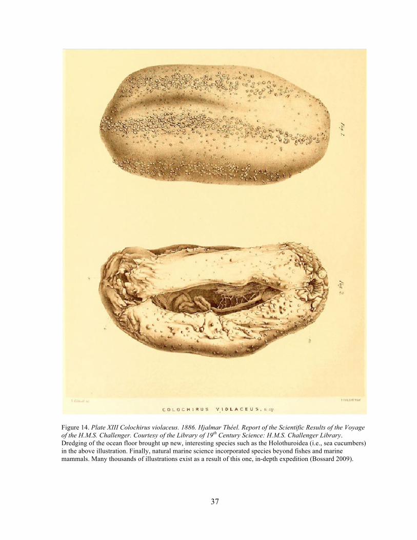
Figure 14. Plate XIII Colochirus violaceus. 1886. Hjalmar Théel. Report of the Scientific Results of the Voyage of the H.M.S. Challenger. Courtesy of the Library of 19th Century Science: H.M.S. Challenger Library. Dredging of the ocean floor brought up new, interesting species such as the Holothuroidea (i.e., sea cucumbers) in the above illustration. Finally, natural marine science incorporated species beyond fishes and marine mammals. Many thousands of illustrations exist as a result of this one, in-depth expedition (Bossard 2009).

38

Figure 15. Echinoidea. Ernst Haeckel. Art Forms in Nature. Haeckel’s plates always achieved an intriguing composition. He managed to balance out the complicated parts of different organisms so the product was not too busy. Haeckel incorporated impressive depth of details, including patterns and anatomical features that brought lifelikeness into his work. The remarkable quality is evidence of the passion he felt for both the discovered science and created art.

39

Figure 16. A visual compendium of glowing creatures. 2014. Eleanor Lutz. Courtesy of TableTopWhale.com Eleanor Lutz began infusing science and art as an experiment following her college graduation. She thoroughly researches a topic of interest; for this one she used over 200 sources to ensure accuracy (Lutz 2014). The significance of this accomplishment is the ability to summarize all that information into a single, aesthetically pleasing and understandable infographic. That is a key purpose of scientific illustration: to communicate complicated ideas through visual expression.

40

Figure 17. Seafloor of George’s Bank. 2001. MJ Brush. Courtesy of NOAA. Depicted here is the artist’s interpretation of a slope making up the wall of Oceanographer Canyon. The artist watched hours of video taken by Alvin so he could portray the seafloor accurately. Photography would not work in this instance as the flashlight only illuminates a fraction of the floor at a time and the scope of the submarine terrain would be lost (NOAA 2010).

41

Figure 18. Chemistry of Ocean Acidification. 2017. Julia Mackin-McLaughlin [Digital image] A portion of CO2 released into the atmosphere is absorbed by the ocean. The series of reactions begins when CO2aq and H2Oaq form carbonic acid (H2CO3). Next, a hydrogen ion (H+) dissociates and H2CO3 becomes bicarbonate (HCO3

2-). This repeats with bicarbonate as another H+ dissociates and HCO32- becomes carbonate

(CO32-). The increase in H+

aq reduces the ocean pH level.

42

Figure 19. Classes of Echinodermata. 2017. Julia Mackin-McLaughlin [Digital image of original oil painting on canvas] Echinoderms are exclusively marine animals characterized by their pentamerous radial symmetry and also their structural use of calcite. Each class uses dermal ossicles embedded in their tissue, but the difference lies in the shapes. Asteroidea and Holothuroidea (top and bottom left, respectively) ossicles are smaller than the armor plating of the Opiuroidea and Crinoidea (top and bottom right, respectively). Echinodea (top center) have enlarged and closely fitted calcareous plates that form a test, or rounded endoskeleton (Pearse et al 1987).

43

Figure 20. Ophiura Plating. 2017. Julia Mackin-McLaughlin. [Digital Photo of Specimen] Example of the calcium plates in an ophiuroid species, Ophiura sarsi. The plates are extensive over the entire body, but still allow for full movement of the animal’s arms. Also evident is pentaradial symmetry: the animal is divisible symmetrically in five separate parts, each 72º apart.

44

Figure 21. Larval Spicule Illumination. 2017. Julia Mackin-McLaughlin [Digital image of original oil painting on canvas] Echinoderm larvae contain spicules made of magnesium calcite which have numerous functions including structural support, maintenance of body shape, and assistance in feeding (Dupont et al. 2008). Polarized light microscopy illuminates larvae spicules. Shown here is a Strongylocentrotus droebachiensis larvae (left) and an Ophiothrix fragilis larvae (right) with visible spicules.

45

Figure 22. Adult Biometric Measurement Standards. 2017. Julia Mackin-McLaughlin [Digital image of original ink drawing on Stonehenge paper with translucent overlays] Standard used for biometric measurements of adult echinoderms exposed to various pH treatments (Stumpp et al. 2012). To assess the impacts on growth, researchers measured the test diameter of S. droebachiensis (left) and arm length of A. rubens measured from the madreporite to the tip of the arm directly opposite. Because gonads are found in the arms of A. rubens, arm length also impacts gonad mass.

46

Figure 23. Larval Biometric Measurement Standards. 2017. Julia Mackin-McLaughlin [Digital image of original ink drawing on Stonehenge paper with translucent overlays] Standard used for biometric measurements. (Above) S. droebachiensis 8-arm pluteus larvae measured with the following: total body length (BL); stomach vertical and horizontal diameter (S); arms’ lengths: postoral (POL), aterolateral (AL), and posterodorsal (PDL) (Dorey et al 2013). (Below) O. fragilis 8-arm pluteus larvae measured with the following: body length (BL); body rod length (BRL); posterolateral rod length (PLL); overall length (OL) (Dupont et al. 2008).

47

Figure 24. Asymmetry and Abnormalities in Ophiothrix fragilis. 2017. Julia Mackin-McLaughlin [Digital image of original oil painting on canvas] Examples of abnormalities and asymmetry in Ophiothrix fragilis larvae found after day 2 of exposure to acidified conditions. Treatments include pH = 7.7 (Top center & bottom right) and pH = 7.9 (bottom left). Larval spicules illuminated using polarized light (Dupont et al 2008).

48

Figure 25. Calcite Armor of Ophiura ophiura. 2017. Julia Mackin-McLaughlin [Digital image of original ink drawing on Stonehenge paper] O. ophiura uses Mg-calcite to build armored plates over its entire body, just beneath its epidermis. These plates provide protection against predators, such as the dabs, reducing the number of arms nipped off. This organism is currently regenerating one of its arms. The armor also allows it the advantage of not having to build a burrow, an energetically costly process.

49

Figure 26. Asterias rubens consuming Mytilus edulis.2017. Julia Mackin-McLaughlin [digital image of original oil painting on canvas] A. rubens is a keystone predator of mussels in the intertidal zone. Previous research established that extensive beds of blue mussels (Mytilus sp.) declined after the introduction of A. rubens (Saier 2001). An A. rubens is able to climb over mussel beds, using their tube feet to attach onto the shell of a mussel. The lattice structure of ossicles retains rigidity through the tissue connecting it. The sea star then everts its stomach to digest the prey within its own shell (Barkhouse et al. 2007).

50

ARTIST’S STATEMENT

The main purpose of this work is to reinforce the critical role scientific illustration has

in marine natural sciences. It is not cliché to say a picture is worth a thousand words.

Illustration offers a way to clarify the sometimes difficult concepts science presents. For

example, I was for a while confused on how A. rubens is able to pull apart a bivalve’s shell

using its tube feet and maintaining rigidity in its arms. It was not until I watched an

animation demonstrating the process that I could actually visualize the ossicles structures.

The animation also possessed an attractive quality, presenting details in a manner that was

both informative and fun to watch. This is a key quality to illustration: a way to draw

attention to information through pleasing aesthetics.

The challenge is that illustration is not an easy process. The amount of effort and time

that goes into creating an effective piece of art is substantial, which I underestimated.

Moving through each step requires thoughtfulness and diligence. My sketchbook was my

best friend, as early planning saved time in later stages, as well as contributing to a better

product. For even a single concept, I scribbled dozens of sketches in search of the perfect

composition. I needed to find the drawing that was effective, but it gets frustrating. Over and

over I tried different subjects, but sometimes what seems an initially great idea never finds its

fruition.

I employed technical skills, such as construction with a compass and ruler, to capture

the pentaradial symmetry attribute shared by all echinoderms. There is a great deal of math

involved; one page of my sketchbook is filled with fractions ensuring the different subjects of

Figure 19 are evenly spaced. This way, I can achieve balance in the image and help guarantee

it is aesthetically pleasing.

51

Usually, I decided what medium I would use for each piece in the early stages. Inks

are tight and allow for higher levels of detail. This was useful for the biometric

measurements in Figure 22 and Figure 23 and the extensive plating of O. ophiura in Figure

25. Figure 22 and Figure 23 posed an interesting challenge in portraying the biometric

standards without cluttering the actual illustration with too much information. To remedy

this, I drew the standards on tracing paper and laid it over the actual specimen illustration,

attaching it only at the top so that it can be lifted and replaced as desired.

Besides Figure 19, the rest of my personal images are oil paintings. Oil paints have a

high flow and this presented a problem in painting as the subject was looser, relative to the

ink pieces. But I have greater experience with oil paints, being my usual medium of choice

when making a piece. For me to jump into a new media, such as watercolor, the end product

would probably suffer a loss in quality as I explored a new medium. I preferred familiarity

and worked with the smoothness of oils to achieve even gradients of color.

Even though I have used oil paints before, painting in general is a new technique I am

learning. Therefore, my confidence in my ability wavered and I became my own worst critic.

I can be demoralizing when working through a piece you only see its mistakes. It can be

demoralizing when working through a piece if you only see its mistakes. I had the mindset

my work would never be good enough to present to my committee. Especially Figure 26,

which ironically now is my favorite piece. It is my favorite because it reminds me of my

personal journey during this Thesis. Through it, I learned you cannot beat yourself up over

your work. Absolutely, you have to accept criticism to improve, but you also have to find

pride in what you do. Otherwise, your confidence will be lost. There is a fine line between

self-criticism and self-confidence and when you find this, you are able to embrace your skill

52

and present your work to the best of your ability. I am glad I undertook this specific project,

as I enjoyed exploring the rich history of a subject I have had interest in for a while. I found

what may be my place in continuing it, as well. I would like to go into scientific illustration

and use my artistic skill to help communicate ecological issues. I am passionate for the

conservation of the natural world, which will be my motivation to help bring about change

for the betterment of the world’s health through illustration.

53

REFERENCES

Appelhans YS, Thomsen J, Opitz S, Pansch C, Melzner F, Wahl M. 2014. Juvenile sea stars exposed to acidification decrease feeding and growth with no acclimation potential. Marine Ecology Progress Series 509:227 – 239.

Barkhouse, C.L., M. Niles, and L.-A. Davidson. 2007. A literature review of sea star control

methods for bottom and off bottom shellfish cultures. Can. Ind. Rep. Fish. Aquat. Sci. 279: vii + 38 p.

Bayliss-Brown G. 2014. How design can be used in science communication. Retrieved from

https://marinescience.blog.gov.uk/2014/06/02/design-science-communication/

Bishop T, Tuddenham P, Ryan M. 2012. Then and Now: The HMS Challenger Expedition and the “Mountains in the Sea” Expedition. Retrieved from http://oceanexplorer.noaa.gov/explorations/03mountains/background/challenger/chall enger.html

Bögner D, Bickmeyer U, Köhler A. 2014. CO2-induced fertilization impairment in

Strongylocentrotus droebachiensis collected in the Arctic. Helgoland Marine Research 68:341 – 356.

Boreham I. 2014. John Reinhold Forster.

http://www.captaincooksociety.com/home/detail/john-reinhold-forster Bossard DC. 2009. H.M.S. CHALLENGER EXPEDITIONS REPORTS ILLUSTRATED

INDEX. Hanover: Dartmouth College. Breidbach O, Hartmaan R, Eibl-Eibesfeldt I, Haeckel E. 2008. Art Forms in Nature: The

Prints of Ernst Haeckel. Munich · London · New York: Prestel. Burns WE. 2001. The Scientific Revolution: An Encyclopedia. Santa Barbara: ABC-CLIO,

Inc. Collard M, Catarino AI, Bonnet S, Flammang P, Dubois P. 2013. Effects of CO2-induced

ocean acidification on physiological and mechanical properties of the starfish Asterias rubens. Journal of Experimental Marine Biology and Ecology 446:355 – 362.

Cook J, Price AG. 1971. The Explorations of Captain James Cook in the Pacific: As Told by

Selections of His Own Journals. Adelaide: Griffin Press. Cosgrove B. 2014. LIFE at Lascaux: First Color Photos From Another World. Retrieved

from http://time.com/3879943/lascaux-early-color-photos-of-the-famous-cave-paintings-france-1947/

54

Da Vinci Science Center. 2003. The Full Story of Leonardo’s Horse. Retrieved from http://www.davincisciencecenter.org/about/leonardo-and-the-horse/the-full-story-of-leonardos-horse/.

Doney SC, Fabry VJ, Feely RA, Kleypas JA. 2009. Ocean Acidification: The Other CO2

Problem. Annual Review of Marine Science 1:169 – 92. Dorey N, Lançon P, Thorndyke M, Dupont S. 2013. Assessing physiological tipping point of

sea urchin larvae exposed to a broad range of pH. Global Change Biology 19:3355 – 3367

Dupont S, Dorey N, Stumpp M, Melzner F, Thorndyke M. 2013. Long-term and trans-life-

cycle effects of exposure to ocean acidification in the green sea urchin Strongylocentrotus droebachiensis. Marine Biology 160:1835 – 1843.

Dupont S, Havenhand J, Thorndyke W, Peck L, Thorndyke M. 2008. Near-future level of

CO2-driven ocean acidification affects larval survival and development in the brittlerstar Ophiothrix fragilis. Marine Ecology Progress Series 373:285 – 294.

Dupont S, Ortega-Martínez O, Thorndyke M. 2010. Impact of near-future ocean acidification

on echinoderms. Ecotoxicology 19:449 – 462.

Fabry J, Seibel BA, Feely RA, Orr JC. 2008. Impacts of ocean acidification on marine fauna and ecosystem processes. ICES Journal of Marine Science. 65:414 – 432.

Hu MY, Casties I, Stumpp M, Ortega–Martinez O, Dupont S. 2014. Energy metabolism and

regeneration are impaired by seawater acidification in the infaunal brittlestar Amphiura filiformis. The Journal of Experimental Biology 217:2411 – 2421.

Keppel EA, Scrosati RA, Courtenay SC. 2014. Interactive effects of ocean acidification and

warming on subtidal mussels and sea stars from Atlantic Canada. Marine Biology Research 11-4:337 – 348.

Langdon C, Takahashi T, Sweeney C, Chipman D, Goddard J. 2000. Effect of calcium

carbonate saturation on the calcification rate of an experimental coral reef. Global Biogeochemical cycles 14(2):639 – 654.

Lebrun D (Producer & Director). 2004. Proteus: A Nineteenth Century Vision [Motion

Picture]. United States: Night Fire Films. Lindsay, SM. 2010. Frequency of injury and ecology of regeneration in marine benthic

invertebrates. Integr. Comp. Biol. 50(3):479-493 DOI: 10.1093/icb/icq099. Lutz E. 2014. A visual compendium of glowing creatures. Retrieved from

http://tabletopwhale.com/page10/.

55

Magee J. 2009. Art of Nature: Three Centuries of Natural History Art from Around the World. Melbourne: Hardie Grant Books.

Meisner G. 2014. Da Vinci and the Divine Proportion in Art Composition. Retrieved from

https://www.goldennumber.net/leonardo-da-vinci-golden-ratio-art/ Natural History Museum. 2010. Cook’s Voyage to the South Seas. Retrieved from

http://www.artstor.org/content/cooks-voyages-south-seas NOAA. 2008. Timeline. Retrieved from

http://oceanexplorer.noaa.gov/history/timeline/timeline.html NOAA. 2010. The Art of Exploration. Retrieved from

http://oceanexplorer.noaa.gov/explorations/deepeast01/background/art/art.html Orr JC, Fabry VJ, Aumont O, Bopp L, Doney SC, et al. 2005. Anthropogenic ocean

acidification over the twenty-first century and its impact on calcifying organisms. Nature 437:681 – 86.

Osterman M. 2013. The Technical Evolution of Photography in the 19th Century. Retrieved

from http://faculty.georgetown.edu/irvinem/theory/Osterman-Romer-history-of-photography-ex.pdf

Paine RT. 1966. Food Web Complexity and Species Diversity. The American Naturalist

100:65 – 75.

Pearse V, Pearse J, Buchsbaum M, Buchsbaum R. 1987. Living Invertebrates. California: The Boxwood Press.

Pendanius D. 99. De Materia Medica. A Laguna (Ed.). Retrieved from World Digital

Library. Popova M. 2012. Natural Histories: 500 Years of Rare Scientific Illustrations from the

American Museum of Natural History Archives. Retrieved from https://www.brainpickings.org/2012/11/27/natural-histories/

Principe LM. 2011. The Scientific Revolution: A Very Short Introduction. United Kingdom:

Oxford University Press. Richards RJ. 2009. Haeckel’s embryos: fraud not proven. Biology Philosophy. 24:147 – 154. Royal Society. 2005. Ocean acidification due to increasing atmospheric carbon dioxide.

Policy Document 12/05, The Royal Society, London. Saier B. 2001. Direct and indirect effects of seastars Asterias rubens on mussel beds (Mytilus

edulis) in the Wadden Sea. Journal of Sea Research 46:29 – 42.

56

State Library of New South Wales. 2016. Sydney Parkinson: The artist’s impressions.

Retrieved from http://www.sl.nsw.gov.au/stories/captain-cooks-voyages- discovery/sydney-parkinson

Stokstad M, Cothren M. 2013. Art History: Volume 1. London: Pearson. Stumpp M, Hu MY, Melzner F, Gutowska MA, Dorey N, Himmerkus N, Holtmann WC,

Dupont ST, Thorndyke MC, Bleich M. 2012. Acidified seawater impacts sea urchin ] larvae pH regulatory systems relevant for calcification. PNAS. 109:18192 – 18197. Suarez MF, Woudhuysen, SJ. 2013. The Book: A Global History. Oxford: Oxford University

Press.

Swetz FJ, Katz VJ. 2011. Mathematical Treasures – De Divina Proportione, by Luca Pacioli. Retrieved from http://www.maa.org/press/periodicals/convergence/mathematical-treasures-de-divina-proportione-by-luca-pacioli

The Metropolitan Museum of Art. 2000. The Art of the Book in the Middle Ages. Retrieved

from http://www.metmuseum.org/toah/hd/book/hd_book.htm Waters H. 2013. The Enchanting Sea Monsters on Medieval Maps. Retrieved from

http://www.smithsonianmag.com/science-nature/the-enchanting-sea-monsters-on-medieval-maps-1805646/

Wood HL, Spicer JL, Lower DM, Widdicombe S. 2010. Interaction of ocean acidification

and temperature; the high cost in the brittlestar Ophiura ophiura. Marine Biology 157:2001 – 2003.

Wood HL, Spicer JI, Widdicombe S. 2008. Ocean acidification may increase calcification

rates, but at a cost. Proceedings of the Royal Society 275:1767 – 1773. Wood HL, Widdicombe S, Spicer JI. 2009. The influence of hypercapnia and the infaunal

brittlestar Amphiura filiformis on sediment nutrient flux – will ocean acidification affect nutrient exchange? Biogeosciences 6:2015 – 2024.

Woods Hole Oceanographic Institution. 2005. History of Oceanography: The Challenger Expedition. Retrieved from http://www.divediscover.whoi.edu/history-ocean/challenger.html

Wyhe JV. 2002. The Complete Works of Darwin Online. Retrieved from http://darwin-

online.org.uk/

57

AUTHOR’S BIOGRAPHY

Julia A. Mackin-McLaughlin was born in Abington, Pennsylvania on February 13th, 1995.

For a portion of her life she lived in Julian, Pennsylvania near Black Moshannon State Park,

before moving to Ambler, Pennsylvania to graduate from Wissahickon High School in 2013.

Majoring in marine science, Julia also has a minor in Studio Art. She spent most of her high

school and University career doodling in sketchbooks instead of listening in class, to the

annoyance of teachers and professors alike. However, it has inspired her to go beyond and try

finding a guild in which to continue scientific illustration.