I II I

III

AEDC- TR-61·4

@

@

HYPERSONIC FLOW-BLAST ANALOGY

By

1. Lukasiewicl

VKF, ARO, Inc.

June 1961

ARNOLD ENGINEERING

D V LOPM NT· CENTER AIR FORCE SYSTEMS COMMAND

u s A F

@

@

ASTIA (TISVV) ARLINGTON HALL STATION ARliNGTON i2, VIRGINIA

Department of Defense contractors must be

established for ASTIA services, or have

their need-to-know certified by the cogni­

zant mi litary agency of their project or

contract.

AF - AEDC Arnold AFS Tenn

HYPERSONIC FLOW-BLAST ANALOGY

By

J. Lukasiewicz

VKF, ARO, Inc.

June 1961

Program Area 750A, Project 8952, Task 89512 ARO Projects 300116, 360105, 360106

Contract No. AF 40(600)-800 S/A 11(60-110)

AEDC·TR.61.4

A EDC·T R·6 1·4

ABSTRACT

Two-dimensional and axisymmetric1 inviscidl hyper­sonic flows about simple slender bodies are considered with particular reference to pressure distributions and shapes of shock waves. Approximate solutions l based on blast analogy, are derived and compared with more exact, theo­retical calculations and with experimental results. The validity of correlation parameters predicted by the blast analogy and the range of their applicability are investigated. Near-exact theoretical results available for real airflow at Mach numbers from 15 to 19 are compared with the perfect gas data.

3

CONTENTS

ABSTRACT .... NOMENCLATURE. INTRODUCTION. . BASIS OF BLAST ANALOGY. APPROXIMATE SOLUTIONS OF UNSTEADY, PLANE

AND CYLINDRICAL, CONSTANT ENERGY FLOW. . First Approximation . . . . . . . . . . Second Approximation. . . . . . . . . . . . . Some Properties of Approximate Solutions . . . .

APPROXIMATE STEADY-FLOW SOLUTIONS BASED ON BLAST ANALOGY ..

First Approximation . . . . . . . . . . Second Approximation. . . . . . . . . . .

SUMMARY OF BLAST ANALOGY SOLUTIONS FOR y '" 1.4 • . . . • . • • . . . • • • •

OTHER BLAST AND STEADY - FLOW SOLUTIONS COMPARISON OF THEORETICAL AND EXPERIMENTAL

RESULTS WITH APPROXIMATE SOLUTIONS. . Plane Flow . . . . . . Axisymmetric Flow.

CONCLUDING REMARKS .. REFERENCES ....•

TABLES

1. Values of Coefficients in the First and Second Approximations to the Blast Solution, y '" 1.4, K '" 0 (Sakurai, Refs. 4, 5). .. ..•.

2. Values of Jo (Sakurai, Ref. 4). . . . . . .

3. Ratio of Pressure at Shock to Pressure at Origin, y = 1.4 • . . . • . . . • • • •

4. Variation of Coefficients for First and Second Approximations with K, for Plane and Cylindrical Flow, Y = 104 • . • • . • • • . • • • • . • • •

AEDC·TR·61·4

Page

3 9

11 11

13 13 15 17

19 20 22

26 27

29 29 31 36 37

16

17

17

18

5. Values of Constants a and b for Various Ranges of pip • 23 00

6. Pressure Ratios at Same x/d (a = 0, y = 1.4, First and Second Approximations) . . . . . . . . . . . . . . 24

5

AEDC-TR·6T.4

Table

7. Pressure Ratios at Same x/d (a = 1, Y = 1.4, First and Second Approximations). . . . . . . . . 26

8. Values of Coefficients in the First Blast-Wave Approximation (y = 1.4) • 28

9. Values of x' (MR = 2.11) • • • • • 33

10. GE Calculations of Flow Fields around a Hemisphere-Cylinder in Real Air in Equilibrium. 35

ILLUSTRATIONS

Figure

6

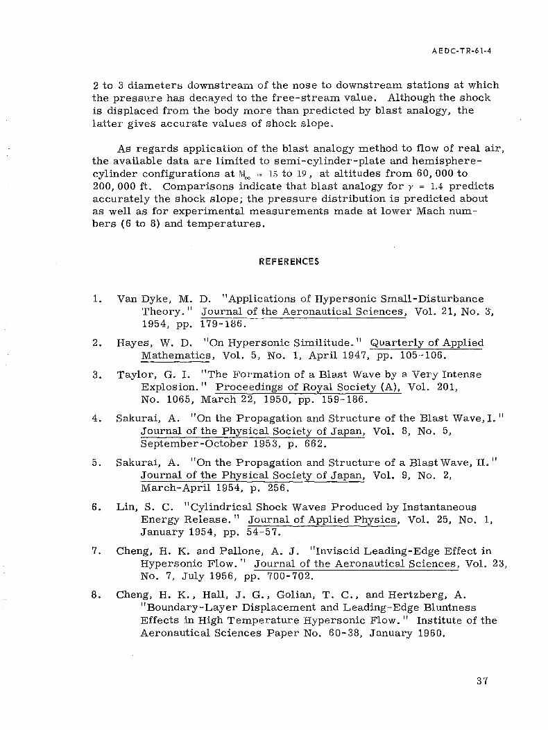
1. Comparison of Pressure Ratios as Given by the First and Second Blast Analogy Approximations at a Given x/d Station (y = 1.4) • • • • • • • • • • • • •• 39

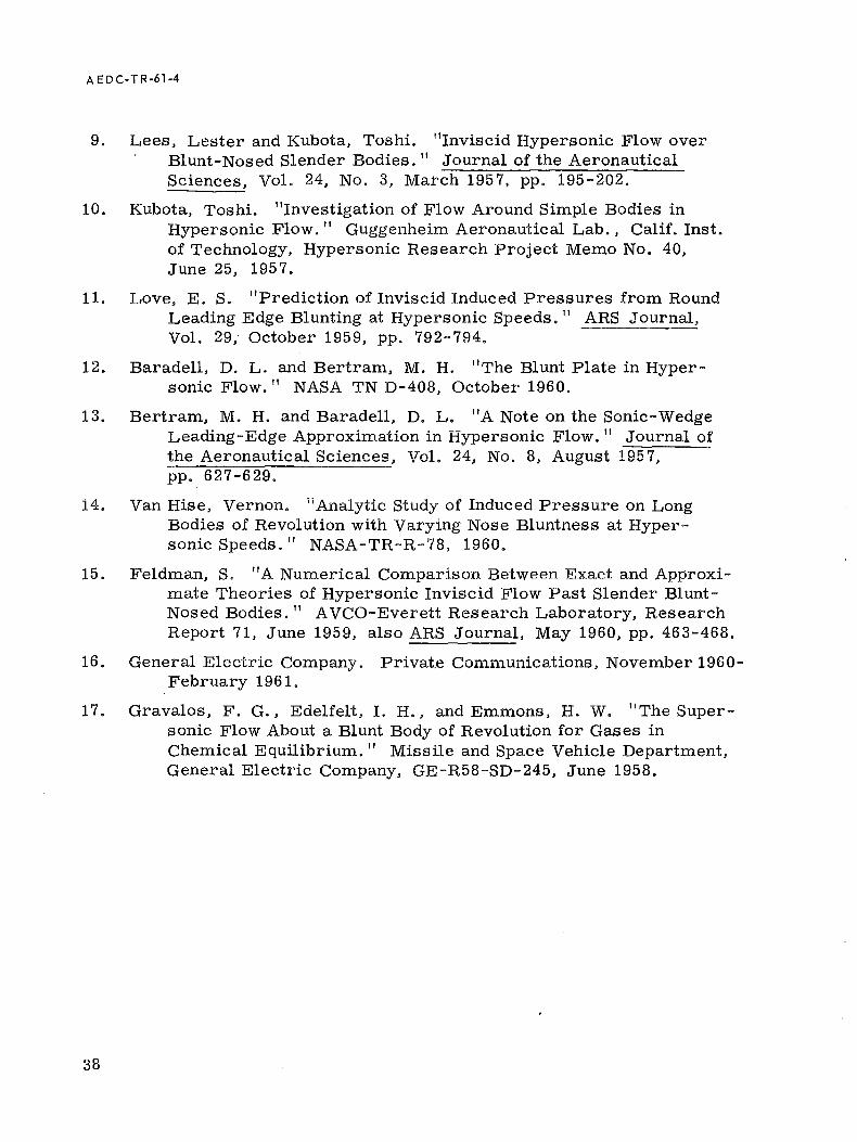
2. Experimental and Predicted Pressure Distribution in Plane Flow, Moo = 8 • • • • • • • • • • • • • • 40

3. Pressure Distribution Calculated by the Method of Characteristics and Blast Analogy in Plane Flow, Moo = 6.86

a. x/d < 35 b. x/d < 200

4. Shock Shapes Calculated by the Method of Characteristics and Blast Analogy in Plane Flow,

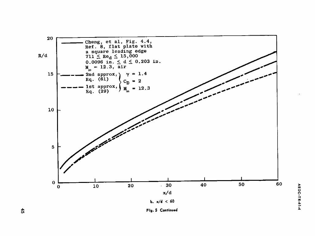
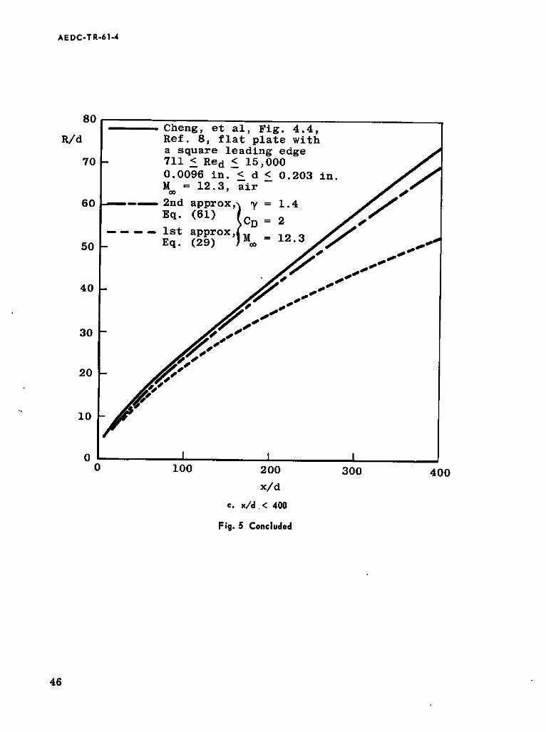
5. Experimental and Predicted Shock Shapes in Plane Flow, Moo = 12.3

a. x/d < 15. b. x/d < 60.

c: x/d < 400

6. Pressure Distributions in Plane Flow Calculated by the Flow Field Method for Real Air and by Blast Analogy,

41 42

43

44 45 46

Moo = 15 • . • . . . • . . • • . . • . . . • • lit 47

7. Shock Shapes in Plane Flow Calculated by the Flow Field Method for Real Air and by Blast Analogy, Moo = 15 II • D • • • • • • • • " • • • • • • • • 48

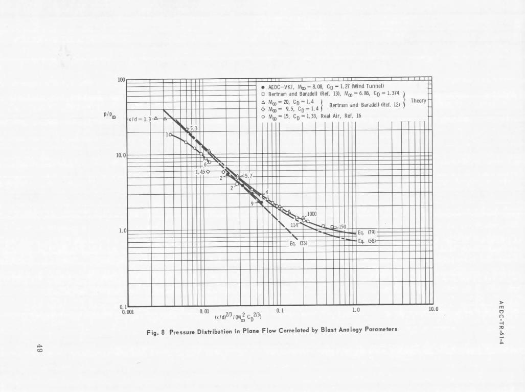
8. Pressure Distribution in Plane Flow Correlated by Blast Analogy Parameters. . . . . . . . . . . . 49

AEDC·TR·61.4

Figure

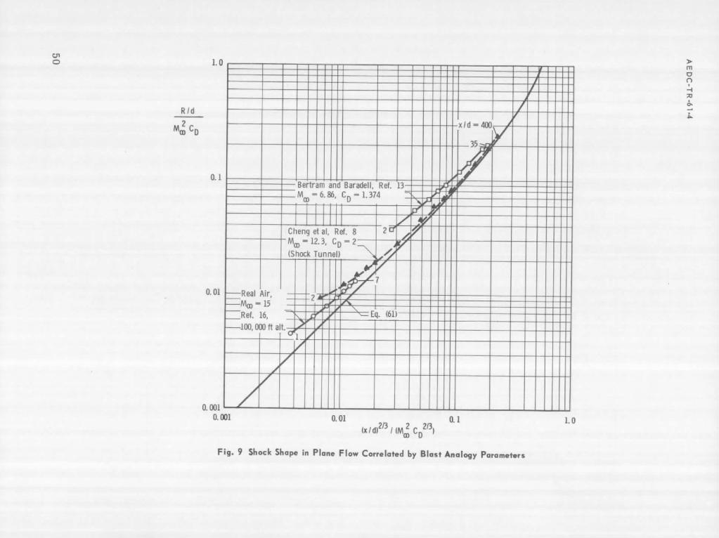
9. Shock Shape in Plane Flow Correlated by Blast Analogy Parameters. . . . . . . • . . . . 50

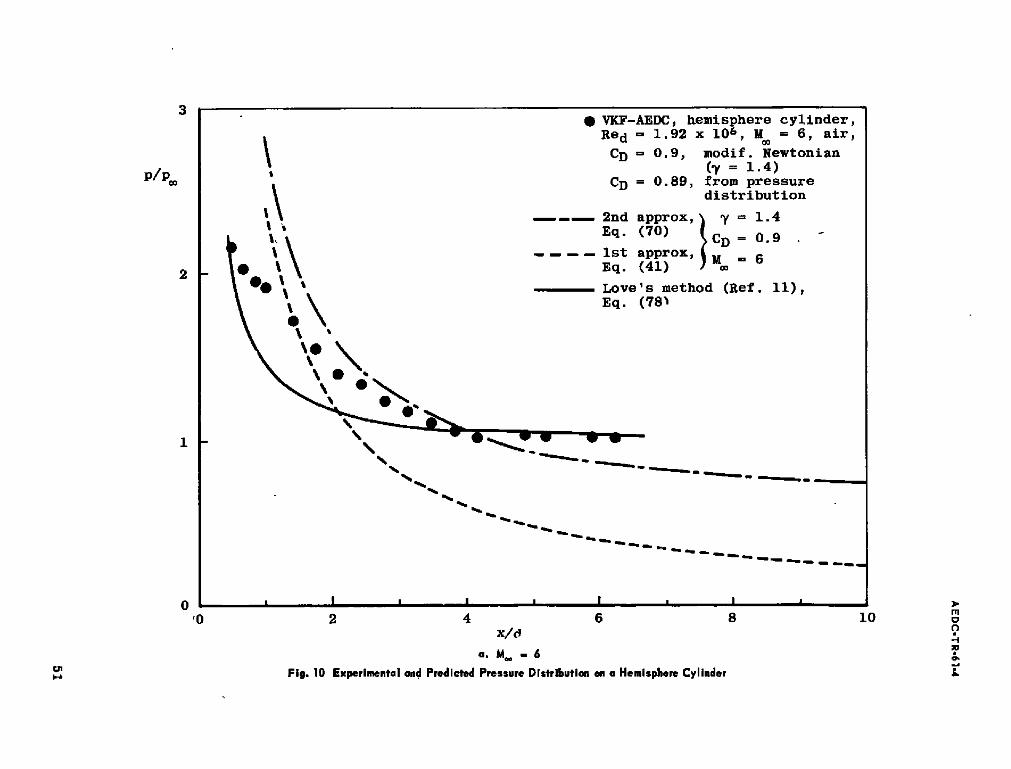
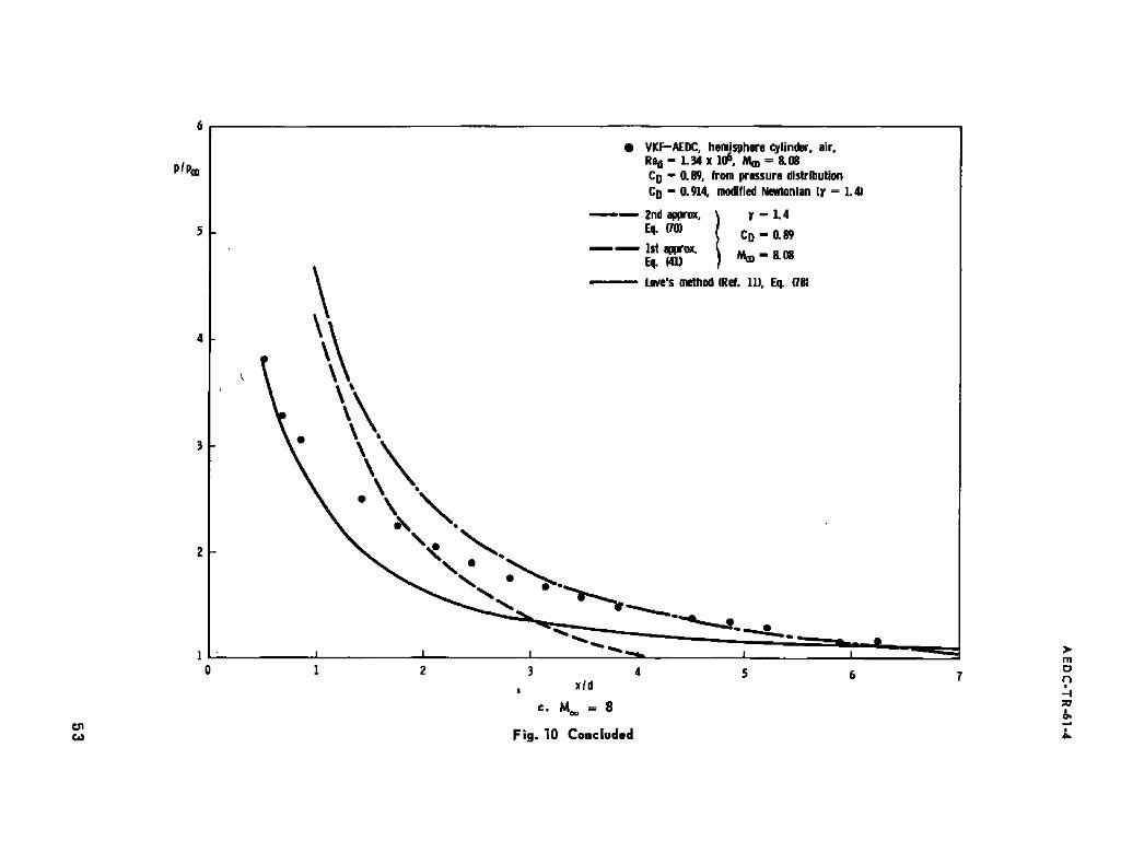
10. Experimental and Predicted Pressure Distribution on a Hemisphere Cylinder

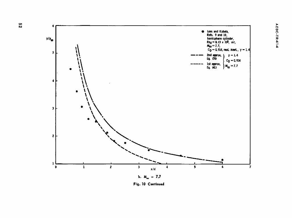
a. Moo 6. 51 b. Moo = 7.7. • • 52 c. Moo = 8 ••••• 53 .

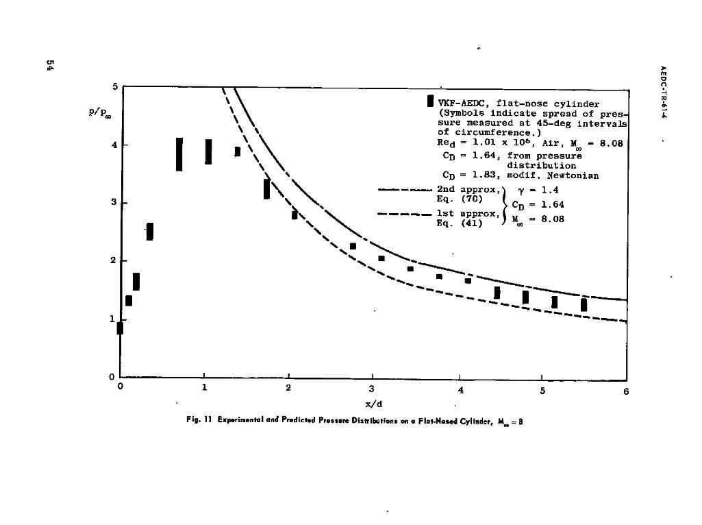
11. Experimental and Predicted Pressure Distributions on a Flat-Nosed Cylinder, Moo = 8 • • • • • • • • • • 54

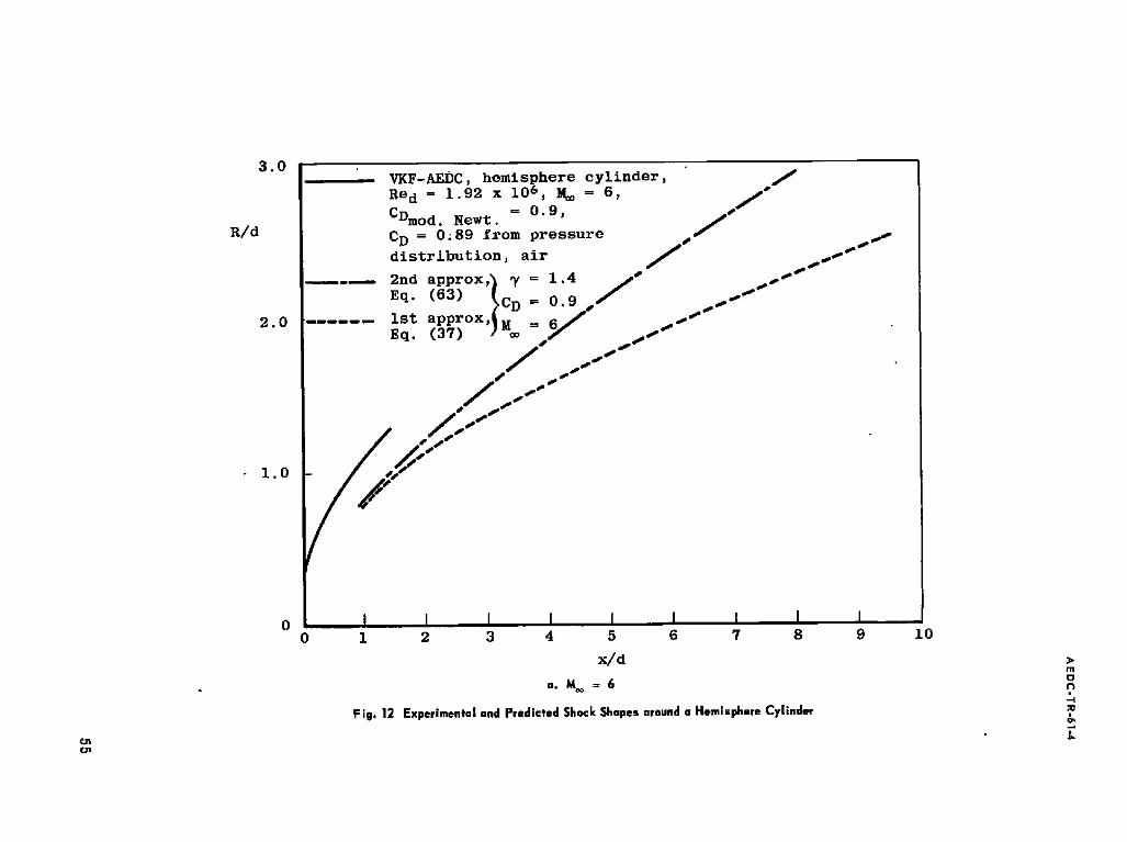
12. Experimental and Predicted Shock Shapes around a Hemisphere Cylinder

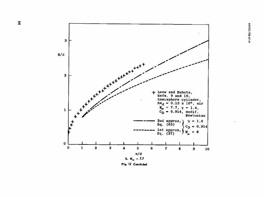
a. Moo = 6. • • • • • • • • • • • • • • • • 55 b . Moo = 7.7. • • • • • • • • • • • • • • • • 5 6

13. Radial Pressure Distribution around a Hemisphere Cylinder at M"" = 7.7, x/d = 3. • • • • • • • • • •

14. Radial Density Distribution around a Hemisphere Cylinder at Moo = 7.7, x/d = 3. • • • • • • • • •

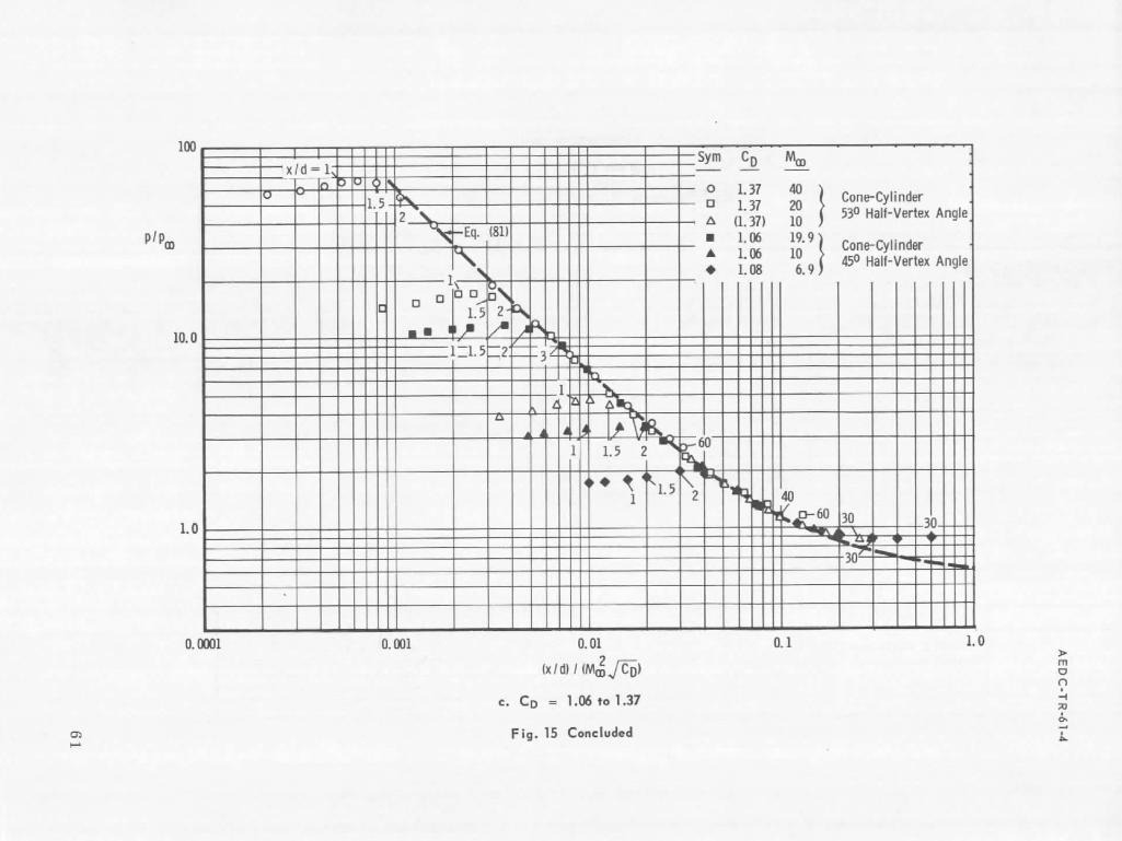
15. Correlation of Theoretical Pressure Distribution in

16.

17.

18.

19.

20.

Axisymmetric Flow for y = 1.4, Ref. 14 a. Moo 40....

b. CD = 0.79 and 0.87 ••. ~ • • •

C. CD == 1.06 to 1.37. • • • • • • • •

Limits of Validity of Blast Analogy Correlation for Various Drag Coefficients, y = 1.4 (Based on Computations by Van Hise, Ref. 14). . . . . . 0

Limit of Validity of Blast Analogy Correlation at Moo = 40,

y = 1.4 (Based on Computations by Van Hise, Ref. 14) . .

Correlation of Theoretical (Method of Characteristics, y = 1.4) Shock Shapes in Axisymmetric Flow . . . . .

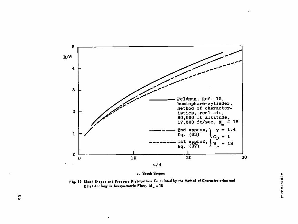
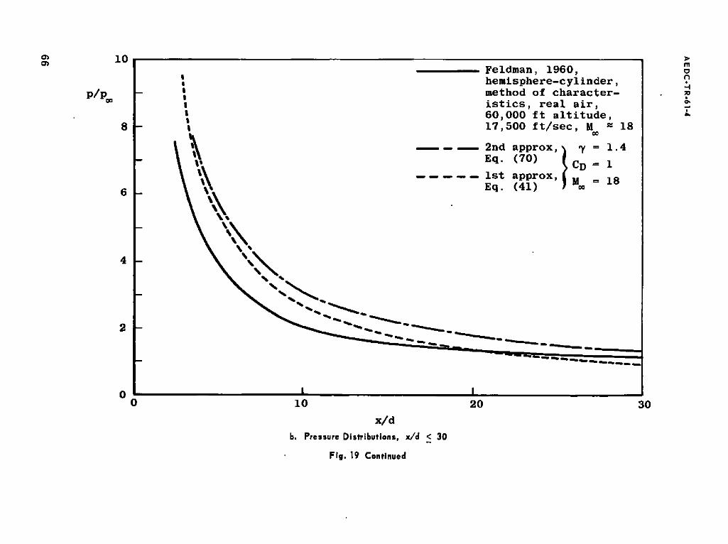
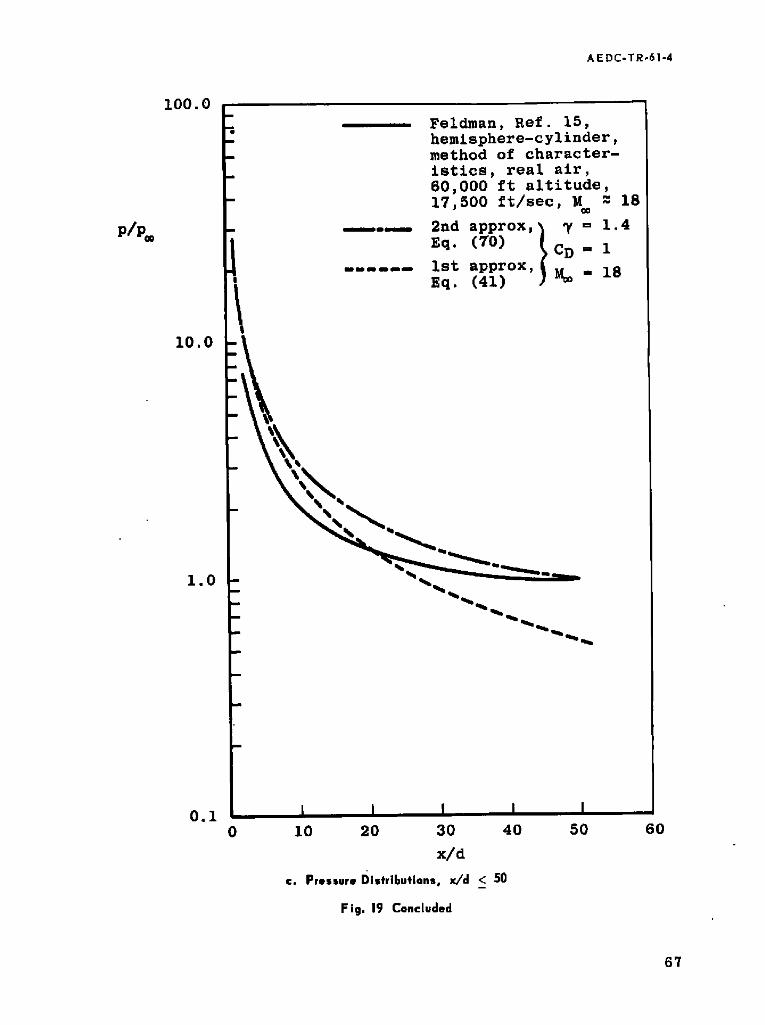
Shock Shapes and Pressure Distributions Calculated by the Method of Characteristics and Blast Analogy in Axisymmetric Flow, Moo ~ 18

a. Shock Shapes. . . . . . . . b. Pressure Distributions, x/d ::; 30 •

c. Pressure Distributions. x/d .::; 50 •

Shock Shape for a Hemisphere Cylinder at Moo = 15 in Real Air . . . . . . . . . . . . 0 • • • • • •

57

58

59 60 61

62

63

64

65 66 67

68

7

AEDC·T R·61.4

Figure Page

21. Pressure Distribution on a Hemisphere Cylinder at Moo = 15 in Real Air . . . . . . . . . . . . . . . •. 69

22. Shock Shape for a Hemisphere Cylinder in Real Air at M.,., = 18.1. • • • • • • • • • • • • • • • • • • • •• 70

23. Pressure Distribution on a Hemisphere Cylinder at Moo ." 18.1 in Real Air. . . . . . . . . . . . . . . .. 71

24. Correlation of Experimental and Theoretical (for Real Air) Pressure Distribution in Axisymmetric Flow .. 72

25. Correlation of Pressure Distribution in Axisymmetric Flow of Real and Ideal (y = 1.4) Air. . . . . . . .. 73

26. Correlation of Experimental and Theoretical (for Real Air) Shock Shapes around a Hemisphere Cylinder. 74

2'7. Radial Pressure Distribution in Flow of Real Air. 75

28. Radial Density Distribution in Flow of Real Air. . 76

8

A,B

a

a, b

c

f, g, h

M

P' o

r

s

u

v

v

x

x P

AEDC·TR·61.4

NOMENCLA TURE

Functions, Eq. (62)

Velocity of sound

Constants

Function, Eq. (64)

Drag coefficient

Drag

Plate thickness or cylinder diameter

Explosion energy per unit area of the surface of shock front when R = 1

Functions, Eq. (3)

Constant

Mach number

Mach number component normal to shock front

Shock Mach number ( = V lao.,)

Static pressure; pressure on plate or cylinder surface

Pitot pressure

Shoulder pressure

Pressure at shock

Distance from shock to origin

(Ea./p",,) 1/(a + 1)

Radial or normal co-ordinate

Distance measured along shock

Time

Velocity component in the free-stream flow direction

Velocity of blast wave

Velocity component normal to the free-stream flow direction or flow velocity caused by explosion

Distance from nose in the free-stream flow direction

Distance from shoulder in the free-stream flow direction

9

AEDC·TR·61·4

y

a

(3,v

y

p

r

<I>, X, tfr

x'

SUBSCRIPTS

00

SUPERSCRIPTS

) ,

)"

10

-2

MR

Constant; = 0 for plane flow,

Functions, Eq. (13)

Ratio of specific heats

rlR

Density

Body thickness parameter

Functions, Eq. (8)

Function, Eq. (76)

Free stream

First approximation

Second approximation

1 for axisymmetric flow

AE DC·TR·61·4

INTRODUCTION

This report deals with the problem of inviscid hypersonic flow of air over simple slender bodies. Two-dimensional and axisymmetric flows are considered with particular reference to pressure distributions and shapes of shock waves. Approximate solutions, based on blast analogy, are derived and compared with more exact, theoretical calcu­lations and with experimental results. The validity of correlation param­eters predicted by the blast analogy and the range of their applicability are investigated. Near-exact theoretical results available for real air­flow at Mach numbers from 15 to 19 are compared with the perfect gas data.

The author wishes to thank Messrs. H. W. Ridyard, R. E. Geiger, and the General Electric Company for permission to use their unpublished flow field computations and Mr. Vernon Van Hise of the NASA Langley Research Center for making his original data available. His thanks are also due to Miss P. Mitchell and Mrs. B. Majors for their help with the preparation of this report.

BASIS OF BLAST ANALOGY

The equations of small disturbance theory of steady, hypersonic flow (Ref. 1) may be written as:

Continuity:

UooPx + (pv)r + apv Ir 0

Momentum:

o ( 1)

Energy:

Uoo (pp -Y)x + v (pp -Y)r = 0

with a = 0 for plane and a = 1 for axisymmetric flow.

As pointed out by Van Dyke (Ref. 1) and Hayes (Ref. 2). these equa­tions do not involve the streamwise velocity u, and therefore the flow in the transverse planes can be treated independently.

Manuscript released by author April 1961.

11

AEDC·TR·61·4

The equations of one-dimensional, unsteady flow are:

Continuity:

Pt + (pv)r + apv/r 0

Momentum:

o (2)

Energy:

(PP-Y)t + v( PP-Y)r = 0

Hay~s (Ref. 2) pointed out that the steady flow, as described by the small disturbance theory, is analogous to the unsteady flow, since, by putting Uoo = dx/dt, Eq. (1) becomes identical with Eq. (2). In other words, for an observer stationary with respect to the undisturbed fluid, the small disturbance theory flow is given by the unsteady solution in one fewer space co-ordinates, so that flow in the plane normal to the direction of motion can be treated independently of x.

If a solution could be obtained for the simpler unsteady problem, then the corresponding steady-flow problem could also be solved; this procedure has been generally known as the blast-wave analogy method. Before this method is applied herein, it is pertinent to recognize the assumptions inherent in the steady and unsteady solutions involved and to examine their compatibility.

The hypersonic small disturbance theory is applicable to slender bodies, such that the body thickness parameter r« 1 (since terms of the order of r2 are neglected), and at large Mach numbers, such that MooT :2: 1. Since the longitudinal velocity component is eliminated in this approximation, the drag of a body is given entirely by the energy of the transverse flow: the drag work expended by moving the body to a given transverse plane is equal to the increment of energy of the transverse flow up to that same plane. The energy of the flow in the transverse plane per unit length will not change when the slope of the body surface is zero; therefore, within the hypersonic, small disturbance approxima­tion, the energy of the transverse flow will remain constant downstream of the forebody or nose when it is followed by a zero-slope afterbody, such as a flat plate or cylinder.

Turning now to the case of unsteady flow, approximate solutions for the spherical, cylindrical, and plane unsteady flows with constant energy have been obtained for cases in which the shock wave which contains the flow field is strong, the shock Mach number being large.

12

AEDC·T R·61-4

Consider a configuration consisting of a blunt nose followed by a zero-slope, flat plate or cylindrical afterbody at a large flight Mach number. For such a body, the hypersonic small disturbance theory will not apply in the nose region, since T « 1 is violated in that region. Also, it will not apply far downstream, where the shock has decayed and flow deflections are negligible, because no longer is MooT;:: 1. There­fore, for a body of this type, the hypersonic, small disturbance theory will apply in a region of certain limited extent downstream of the nose. In this region, the body surface slope is zero, the energy in the trans­verse plane is constant. and hence the unsteady solutions are applicable. The success of the blast-wave analogy will thus largely depend on the accuracy of the solutions of unsteady, constant energy flows.

APPROXIMATE SOLUTIONS OF UNSTEADY, PLANE AND CYLINDRICAL, CONSTANT ENERGY FLOW

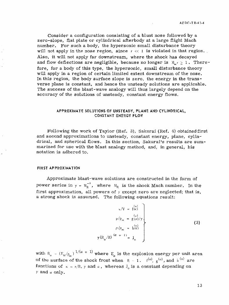
Following the work of Taylor (Ref. 3), Sakurai (Ref. 4) obtained first and second approximations to unsteady, constant energy, plane, cylin­drical, and spherical flows. In this section, Sakurai's results are sum­marized for use with the blast analogy method, and, in general, his notation is adhered to.

FIRST APPROXIMATION

Approximate blast-wave solutions are constructed in the form of

power series in y = M;2. where MR is the shock Mach number. In the

first approximation, all powers of y except zero are neglected; that is, a strong shock is assumed. The following equations result:

(0 ) v/V = f(K)

p/Poo (0 )

g (K)/Y

(0 ) ( 3)

p/Poo h(K)

(R /R) (a + 1)

10 y 0

with Ro = (Ea/Poo) l/(a + 1) where Ea is the explosion energy per unit area

of the surface of the shock front when R = 1. £(0), g(o), and h (0) are

functions of K = r/R, y and a. whereas 10 is a constant depending on y and a only.

13

A E DC· T R·6 1.4

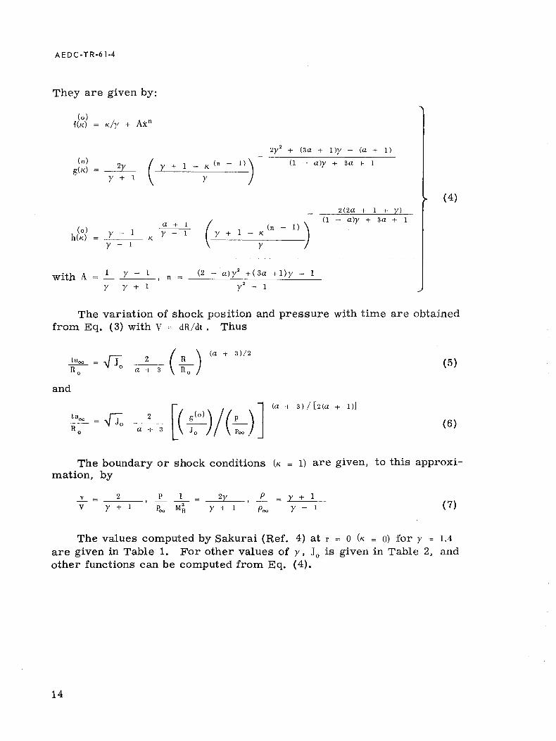
They are given by:

with A

2y y + 1

y + I

Y - 1

a + 1

K Y - 1

I y - I f n

y y + 1

(n -- K

2y2 + (3a + l)y - (a + 1)

(1 - a)y + 3a + 1

y

( (n - I) ) ,J + I - ;

(2 - a)y2 +(3a +I)y - I

y2 _ 1

2(2a + 1 + y) (1 - a)y + 3a + 1

(4)

The variation of shock position and pressure with time are obtained from Eq. (3) with V = dR/dt. Thus

taoo = ·IJ R \I J o

o

and

_2 __ (~) (a + 3)/2

a + 3 Ro (5)

(a + 3) I [2 (a + 1)]

The boundary or shock conditions (K mation, by

..::!...- = _.::...2 __ V y + 1

P I p. M2

00 R

_-'2y'---_, ~ Y + 1 Poo

(6)

1) are given, to this approxi-

y + I

Y - 1 ( 7)

The values computed by Sakurai (Ref. 4) at r = 0 (K = 0) for y 1.4

are given in Table 1. For other values of y J 10 is given in Table 2, and other functions can be computed from Eq. (4).

14

A E DC· T R·6 1·4

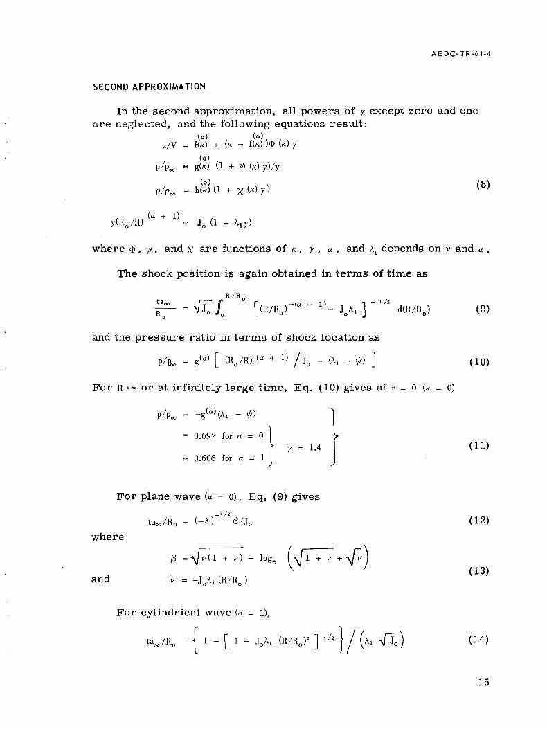
SECOND APPROXIMATION

In the second approximation. all powers of y except zero and one are neglected, and the following equations result:

(0) (0) v/V £(K) + (K - f(K))<1> (K) y

(0) g(K) (l + tjJ (K) y) Iy

(0) h(K) (l + X (K) y) (8)

y(Ro IR) (a + 1) -_ J ( \) o 1 + 1\1 Y

where <l>. tjJ. and X are functions of K, Y. a, and \ depends on y and a •

The shock position is again obtained in terms of time as

R/R

~ = fi:J 0 [(R/R )-<a + 1)_ J A ] -1/2 d(R/Ro) (9) Ro 0 0 0 0 1

and the pressure ratio in terms of shock location as

( 10)

For R-HO or at infinitely large time, Eq. (10) gives at r 0 (K 0)

0.692 for a = 0 }

for a = 1 y 1.4 ( 11)

0.606

For plane wave (a = 0), Eq. (9) gives

( 12)

where

and

f3 = ~ v (1 + v) - loge (.J 1 + v + ~ ) V = -JoA! (R/Ro )

( 13)

For cylindrical wave (a = 1),

( 14)

15

AEDC-TR·61-4

In this approximation, the exact conditions at the shock are satis­fied for velocity and pressure, that is

• v = 2 (1 - y) v y + 1 (15)

P 2y I Y - I = -Poo Y + 1 Y Y + 1 ( 16)

the above equations corresponding to Eq. (8) with

(0) £(1) = __ 2_

y + 1

and (0) (0)

W (l) = - £(I)/(1 - £(I)

The exact density ratio across the shock is

P (Y+I\/( 2 ) Poo = Y - 1)/ 1 + y - 1 Y (17)

This is not equivalent to the corresponding Eq. (8), except for small y

(large MR ), when it is expanded to

with

and

(0) h(I)

y + I

Y - I

x (1) = _ 2 Y - 1

2 ( 18) y - 1

The coefficients in the second approximation are given in Table 1 for r = 0 (K = 0) and y = 1.4.

a

0

1

16

TABLE 1

VALUES OF COEFFICIENTS IN THE FIRST AND SECOND APPROXIMATIONS TO THE BLAST SOLUTION, Y = 1.4, K = 0 (SAKURAI, REFS. 4, 5)

(0) (0) (0) 10 W(o) tjJ(o) X(o) '\1 £(0) g(o) h(o)

0 0.455 0 1. 696 -3.86 -0.617 3.86 -2. 138

0 0.424 0 0.877 -3.5 -0.56 3.5 -1. 989

AEDC·TR·61·4

TABLE 2

VALUES OF Jo (SAKURAI, REF.4)

~ 0 1

1.2 3.024 1. 547

1.3 2. 147 1.102

1. 667 1. 137 0.585

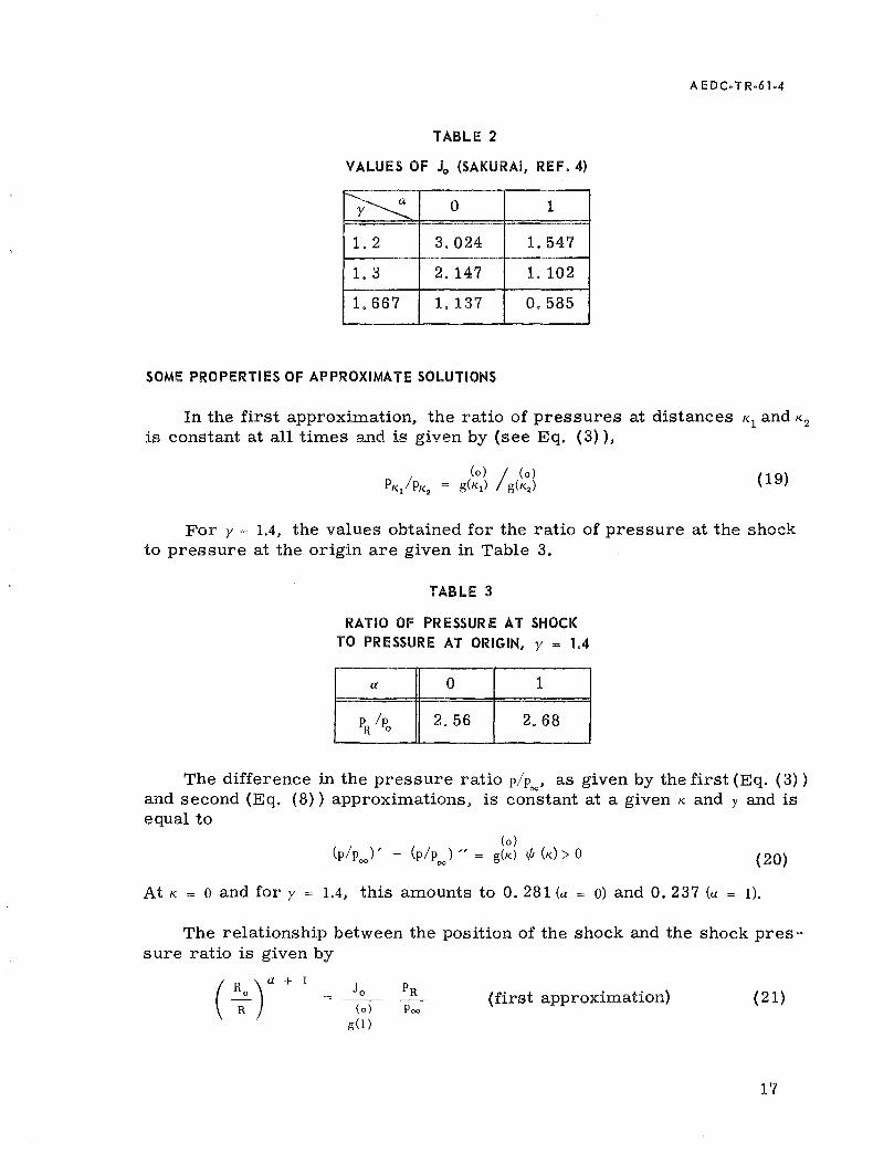
SOME PROPERTIES OF APPROXIMATE SOLUTIONS

In the first approximation, the ratio of pressures at distances Kl and K2

is constant at all times and is given by (see Eq. (3) L

( 19)

For y = 1.4, the values obtained for the ratio of pressure at the shock to pressure at the origin are given in Table 3.

TABLE 3

RATIO OF PRESSURE AT SHOCK

TO PRESSURE AT ORIGIN, y = 1.4

a 0 1

PR Ipo 2.56 2.68

The difference in the pressure ratio pip, as given by the first (Eq. (3» 00

and second (Eq. (8» approximations, is constant at a given K and y and is equal to

(20)

At K = 0 and for y = 1.4, this amounts to 0.281 (a = 0) and 0.237 (a = 1).

The relationship between the position of the shock and the shock pres­sure ratio is given by

(first approximation) ( 21)

17

AEDC-TR-61.4

and ( 22)

(second approximation)

For y 1.4, the second approximation is

a = 0, (R/Ro) (PR /Poo - 2.33) = 0.69}

a = 1, (R/R )2 (p /p - 2.16) = 1.33 o R 00

(23)

In the first approximation, the numerical term in the bracket is omitted.

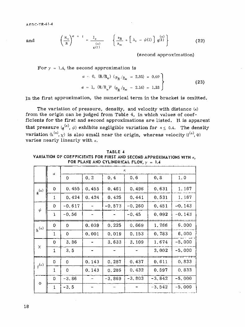
The variation of pressure, density, and velocity with distance (K)

from the origin can be judged from Table 4, in which values of coef­ficients for the first and second approximations are listed. It is apparent

that pressure (g(o), t/J) exhibits negligible variation for K:::; 0.4. The density

variation (h (0), x) is also small near the origin, whereas velocity (£(0), 1» varies nearly linearly with K.

18

TABLE 4 VARIATION OF COEFFICIENTS FOR FIRST AND SECOND APPROXIMATIONS WITH K,

FOR PLANE AND CYLINDRICAL FLOW, y = 1.4

I(

a 0 0.2 0.4 0.6 0.8 1.0

(0) 0 0.455 0.455 0.461 0.496 0.631 1. 167 g

1 0.424 0.424 0.425 0.441 0.531 1. 167

0 -0.617 - -0.573 -0.260 0.451 -'0.143 t/J

1 -0.56 - - -0.45 0.092 -0. 143

h (0) 0 0 0.039 0.225 0.669 1. 766 6.000

1 0 0.001 0.019 O. 153 0.783 6.000

0 3.86 - 3.633 3. 109 1. 674 -5.000 X

1 3.5 - - - 3.002 -5,000

0 0 O. 143 0.287 0.437 0.611 0.833 £(0)

1 0 O. 143 0.286 0.432 0.597 0.833

0 -3.86 - -3.869 -3.803 -3.842 -5.000 lD

1 -3.5 - - - -3.542 -5.000

AEDC·TR·61·4

APPROXIMATE STEADY·FLOW SOLUTIONS BASED ON BLAST ANALOGY

The steady, blast analogy approximations are obtained from the approximate constant energy, blast solutions by superposition of free­stream velocity Uo<> = x/t and by expression of the energy of unsteady flow in terms of body wave drag. Thus the plane blast solution is anal­ogous to two-dimensional flow over a blunted plate, and the cylindrical blast solution corresponds to the case of axisymmetric flow about a blunted cylinder. In each instance, first and second blast approxima­tions are used to obtain approximate steady-flow solutions.

In obtaining steady-flow solutions, the shock shape, R/d, and the pressure distribution, Po /Po<>' on the body surface as a function of distance along the body, x/d, are the main concern. These solutions are strictly applicable only to flat plates and cylinders at zero incidence. The body pressure Po' denoted below by p, is taken at K = O. and the body thick­ness is thus neglected. In view of the invariance of pressure with K and the small density near the origin (see Table 4) this procedure seems reasonable.

Static pressure and other parameters of flow in the transverse plane are easily obtained from blast solutions, provided the shock shape has been determined. Since

(24)

is given from the shock slope, distributions of transverse pressure, density, etc., follow from Eqs. (3) and (8).

It should be noted that, although the second blast-wave approxima­tion gives essentially exact conditions at the shock surface (see Eqs. (15) through (18», the corresponding blast analogy gives correct values of pressure, etc., at the shock only when the component of Mach number, M

n,

normal to the shock, s,

(25)

closely approximates Mn' This, however, is consistent with the assump­tions of the hypersonic small disturbance theory.

For the analogous steady-flow solutions, the blast energy, Ea , is expressed in terms of drag. From the definition of Ea,

Ea=o + Da=o

and

19

AE DC·TR·61.4

where

Da = 0 npse drag of plate per unit length of leading edge

and

Da = 1 = nose drag of cylinder

In terms of drag coefficient, CD'

E = Y d P M2 C a=o 4 00 00 Da=O

and (26)

Ea=l d2 Poo M2 C y 16 00 Da=l

R Ff- M K=l °a= 1 00

where CD is based on plate thickness, d, or cylinder frontal area, 7Td 2/4, and free-stream dynamic pressure.

FIRST APPROXIMATION

From Eqs. (5) and (6), the following expressions for shock, shock slope, and pressure distribution are obtained.

Plane flow (a = 0):

~ = ( : 12/3 (~y/3 CD 1/3 (~12/3

or

for y 1.4;

20

Rid M2 C

00 D

dR = dx

0.774 (xl d) 2/3 C 2/3 M2

D 00

(~)1/3 C 1/3 6J D

o

0.516 CD 1/3 (;) -1/3

(27)

(28)

(29)

( 30)

( 31)

and

for y = 1.4.

From Eqs. (29) and (33),

p/poo = 0.0936 M!, CD / (R/d)

for y = 1.4.

Axisymmetric flow (a =1):

or

for y 1. 4;

and

for y = 1.4.

= 0.795 CD 1/4 (x/d) 1/2

~d_ = 0.795

Moo-fC;;

x/d

= 0.397 CD 1/4 (x/d) - 1/2

= 0.067 M~ ~ I(x/d)

From Eqs. (37) and (41),

for y = 1.4.

A E DC -T R -6 1-4

( 32)

(33)

(34)

(35)

(36)

( 37)

(38)

(39)

( 40)

(41)

( 42)

21

AE DC·TR·61·4

SECOND APPROXIMATION

From Eqs. (10) to (14), the following expressions for shock shape and pressure distribution are derived:

Plane flow (a = 0):

In this case, explicit expressions for shock shape and pressure ratio were not obtained. Thus, for shock shape:

x ~ (-A )-3/2 (3 C M!, d 41 1 D

o

0.066 (3 CD M!,

for y = 1.4

where (3 and v are given by Eq. (13) and

v = -(4Jo A1 /Y) (R/d) / (M~ CD)

for Y = 1.4.

The shock slope is given by

From Eq. (10),

-""" ~.J YCD ~

dx 2 10 ~Ii/d

0.453 ~-rc ~ ~\''-'D

= 0.973 / (p/Poo - 0.692)

( 43)

(44)

(45)

( 46)

(47)

( 48)

( 49)

(50)

for y = 1.4 which, together with Eq. (43) gives pressure distribution.

In the limit when (t, R, x)->oo, the pressure ratio is given by Eq. (11) (= 0.692 for y = 1.4).

The function (3 (Eq. (13», when expressed in terms of pressure ratio p/Poo (Eq. (50», can usually be approximated to better than one per­cent by an expression of the form

(3 = a(p/poo)b

22

AEDC-TR-61-4

where a and b are given, for y

of p/Poo.

1.4, in Table 5 for various ranges

TABLE 5

VALUES OF CONSTANTS a AND b FOR VARIOUS RANGES OF p/Poo

Range of a b

p/Poo

2 - 4 1. 30 -1. 87

4 - 20 0.87 -1. 59

20 - 100 0.69 -1. 52

Using this form of (-3, Equation (43) can be written

x

d

for y 1.4;

or p

for y = 1.4

= [ (I5.I5/al

x/d M3 C

00 D

] lib

which is analogous to the first approximation, Eq. (32).

(51)

(52)

(53)

(54)

A more convenient form of the second approximation for pressure distribution can be derived as follows:

From Eqs. (32), (43), and (49), the pressure ratio (p/Poo )', as given by the first approximation at a given x/d, can be expressed in terms of the second approximation pressure ratio (p/POO)N at the same x/d by

(55)

and

(56)

for y = 1.4

and is therefore a function of (p/poo) N only.

23

AEDC-TR-61-4

The values of

[ (p/poo)", (p/poo)' ] x/d

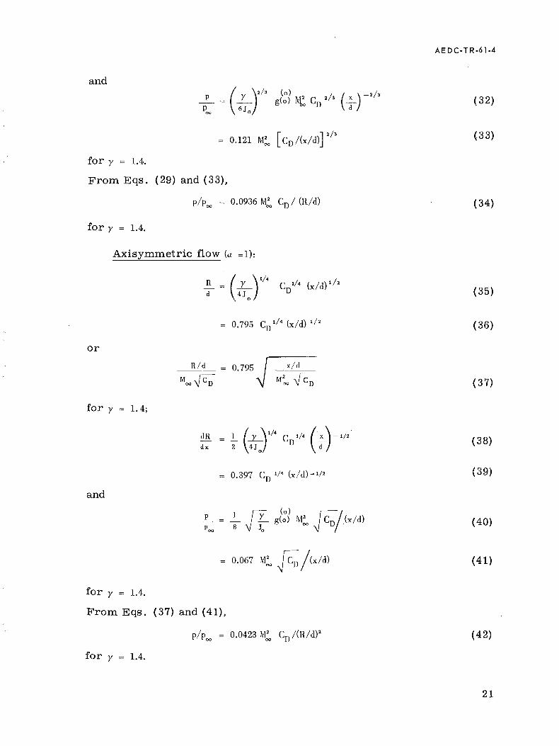
as obtained from Eq. (56), are tabulated in Table 6 and plotted in Fig. 1 in terms of the difference (p/Poo)" - (p/Poo)' vs (p/poo)".

TABLE 6

PRESSURE RATIOS AT SAME x/d (a", 0, y == 1.4, FIRST AND SECOND APPROXIMATIONS)

(p/poo) "x/d 0.692 0.8 1 2 5 10

(p/Poo)'x/d 0 0.191 0.428 1. 473 4.493 9.503

From Fig. 1, it is evident that the simplified expression

(57)

2/3

0.121 M: [ CD/Cx/d) ] + 0.56 (58)

gives the second approximation pressure ratio to better than 1.5 percent when p/poo .2 1, Y = 1.4.

For the shock shape (Eqs. (10) and (26) ),

n d

for y 1.4, and using the simplified expression (Eq. (58»,

for y = 1.4.

n/d M2 C

00 D

0.774

(59)

(60)

(61)

For p/poo ~ 1, this equation gives values to within 4.5 percent of the second approximation (Eq. (44».

Axisymmetric flow (a = 1):

~ = A ~ : ) 1 - 2B : (62)

with

24

A E DC· T R ·6 1·4

and

hence

0.795 2 x/d 1 + 3.15 2x

/d

( )1/2 ( )1/2

Moo rc;; Moo Fn (63)

for y 1.4.

dR = A[C/2 - B/C] dx (64)

with

C = ~ (1 - 2 Bx/d)/(x/d)

(0) [I - r p fi g(o) ycr;12 2A1YY;:- x/d (0) D 00 g(o) (A1 - tjJ)

Poo 8~ x/d ff M!,YC;;

(65)

M!,~ [I ./d ] -. 0.067 + 3.15 + 0.606 x Id M:~

(66)

Using the same procedure as in the case of plane flow, simpler equations for the second approximation are derived. From Eqs. (40) and (65),

( ~oo ) [1 + 0.211/(p/poo)'] _1 + 0.606

for y = 1.4.

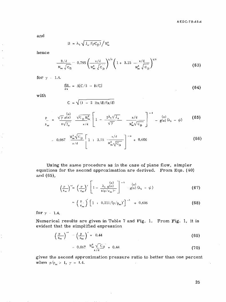
Numerical results are given in Table 7 and Fig. 1. evident that the simplified expression

( :00 )" = ( :00 r + 0.44

= 0.067 M!, y~ + 0.44 x/d

(67)

(68)

From Fig. 1, it is

(69)

(70)

gives the second approximation pressure ratio to better than one percent when p/Poo > 1, y = 1.4.

25

AEDC·TR·61·4

TABLE 7

PRESSURE RATIOS AT SAME x/d (a 1, y = 1.4, FIRST AND SECOND APPROXIMATIONS)

(p/poo)" 0.606 0.958 1. 432 2.415 5.404 10.4

(pip",,) , 0 0.5 1 2 5 10

For the shock shape, Eqs. (10) and (26) give

-d Il = ( 71)

(72)

Using Eq. (69), the simplified expression is

JL = --;=-__ 0_,7_9_5_M_oo_V_C--'D"-----:;--:--

d [Me! v'C;/{X/d)-2, 47Sl/2 (73)

For pip > 1, this expression gives values to better than one percent of "" the second approximation, Eq. (63).

SUMMARY OF BLAST ANALOGY SOLUTIONS FOR Y 1.4

For convenience, the above-derived results for y 1.4 are listed as follows:

Plane Flow

First approximation:

III d

M2 C "" D

= 0.774 (x/d) 2/3

M2 C 2/3 00 D

Second approximation (simplified expressions):

26

III d

M2 C 00 D

0.121

0,774

+ 0.56

(29)

(33)

(61)

(58)

Axisymmetric Flow

First approximation:

Rid 0.795 x/d

Moo {S;

Second approximation:

Exact:

Simplified:

Simplified:

0.795 (2X/d )1/2 (1 + 3.15 X/d) 1/2 Moo Fu M!, {CD

0.067 !vi!, ~ CD + 0.44 x/d

OT-HER BLAST AND STEADY-FLOW SOLUTIONS

A E DC-TR-61-4

( 37)

( 41)

(63)

(73)

(70)

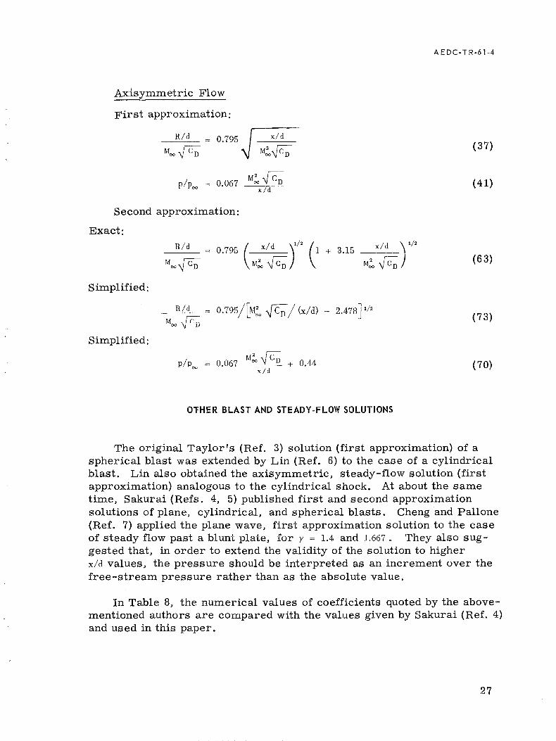
The original Taylor's (Ref. 3) solution (first approximation) of a spherical blast was extended by Lin (Ref. 6) to the case of a cylindrical blast. Lin also obtained the axisymmetric, steady-flow solution (first approximation) analogous to the cylindrical shock. At about the same time, Sakurai (Refs. 4, 5) published first and second approximation solutions of plane, cylindrical, and spherical blasts. Cheng and Pallone (Ref. 7) applied the plane wave, first approximation solution to the case of steady flow past a blunt plate, for y = 1.4 and 1.667. They also sug­gested that, in order to extend the validity of the solution to higher x/d values, the pressure should be interpreted as an increment over the free-stream pressure rather than as the absolute value.

In Table 8, the numerical values of coefficients quoted by the above­mentioned authors are compared with the values given by Sakurai (Ref. 4) and used in this paper.

27

AEDC-TR-61-4

TABLE 8

VALUES OF COEFFICIENTS IN THE FIRST BLAST·WAVE APPROXIMATION (y 1.4)

Coefficient 10 (0)

g(o)

a 0 1 0 1

Sakurai (Ref. 4) 1. 696 0.877 0.455 0.424

Cheng and Pallone (Ref. 7) 1. 121* O. 319

Lin (Ref. 6) 0;858 0.4317

*Cheng et al (Ref. 8) pointed out that this value is in error.

Lees and Kubota (Refs. 9 and 10) applied Sakurai's results to obtain second approximation, steady-flow solutions analogous to the case of cylindrical blast. They derived "simplified" expressions for the case of a hemisphere-cylinder, as follows:

p/Poo = 0.0655 M:/ (x/d) + 0.405

R/d = 0.78 -,J x/d [1 + 1.62 (x/d) / M:']

(74)

(75)

These expressions correspond to the binomial expansion, of Eqs. (66) and (63), using the modified-Newtonian drag coefficient for a hemi­sphere at Moo = 7.7, Y = 1.4 (CD = 0.914).

Love (Ref. 11) proposed a method of calculation of bluntness-induced, inviscid, steady-flow pressures downstream of hemispherical and hemi­cylindrical noses. In his method, a value of the pressure at the shoulder is calculated or assumed, and the pressure decay as given by the first approximation, blast-wave analogy is taken. Love's expression in terms of free-stream pressure, Poo' is as follows:

where

and

(76)

Psh shoulder pressure, i. e., pressure at the juncture of hemi­spherical (or hemicylindrical) nose to the cylindrical (or slab) afterbody;

Po' stagnation point pressure;

x'/d = dimensionless distance measured from the shoulder.

28

A E D C- T R -6 1-4

Theoretical calculations indicate that, at Mach numbers.::: 5, Psh Ipo' re­mains approximately constant and equal to O. 045 in axisymmetric flow and to O. 117 in two-dimensional flow (y = 1.4). The values of exponent a

are taken as 1 and 2/3, respectively, in these two cases, following the blast analogy. Using these values, Love's expressions can be written as follows:

1. hemicylinder - flat plate:

p/poo = 0.117 [1 + (x'/d)2/3J-1

( '/ )+[1 + (x'/d)_2/3]-0.117 po'/Poo Po Poo

2. hemisphere-cylinder:

I ( I) 1 'I + [1 + (x'/d) -1J -0.045 Po '/poo P Poo = 0.045 1 + x' d - Po Poo

The value of Po '/poo is a function of the free-stream Mach number.

COMPARISON OF THEORETICAL AND EXPERIMENTAL RESULTS WITH APPROXIMATE SOLUTIONS

( 77)

(78)

The various blast analogy and other approximations listed above are compared here with three kinds of data:

1. results of theoretical calculations of flow about simple bodies, for ideal and real air;

2. measurements from wind and shock tunnel experiments;

3. results of correlations, in terms of blast-wave analogy param­eters, of theoretically calculated flows.

As regards experimental data, only those measurements made at Reynolds numbers high enough to render the viscous effects negligible are included.

PLANE FLOW

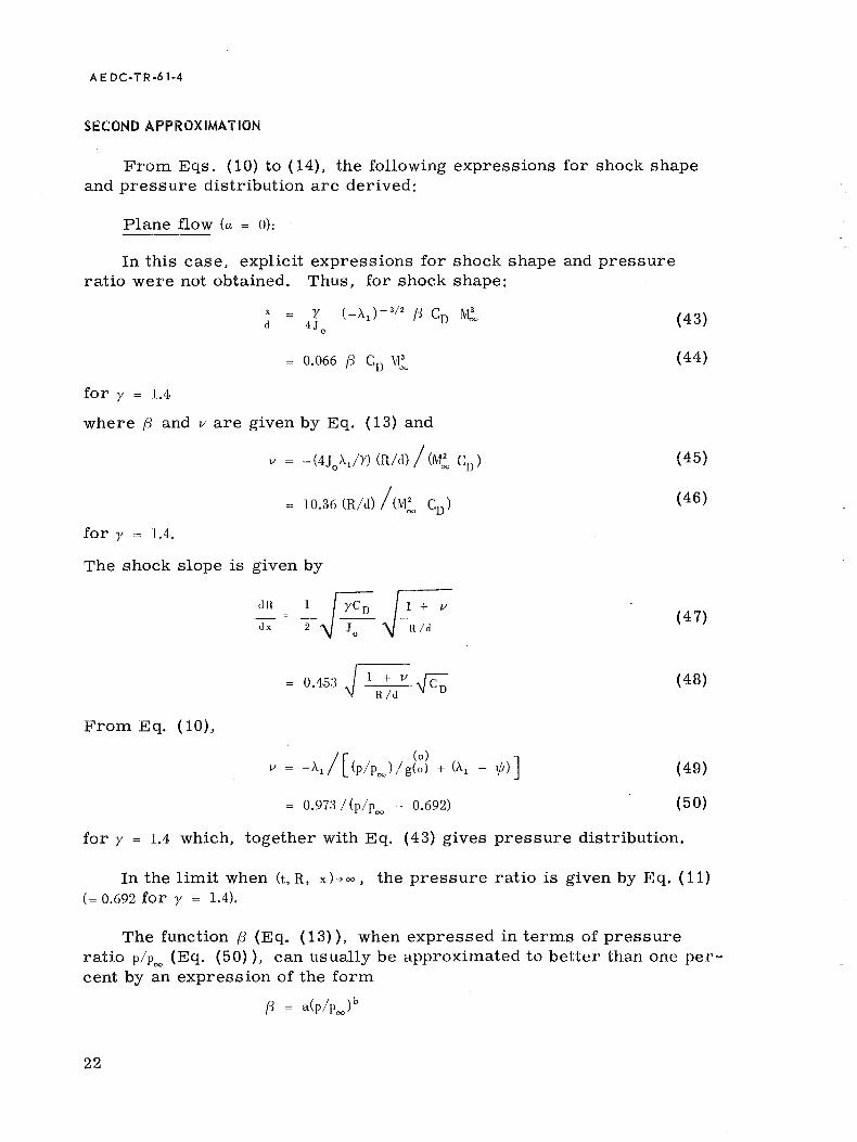
On the basis of calculation (method of characteristics) and correla­tion of flow about flat plates with sonic wedge leading edges, Baradell and Bertram (Ref. 12) suggested the following expression* for pressure distribution (y = 1.4):

( 79)

*This is derived from Eq. (7) of Ref. 12, with (p - Poo)/poo increased by 3 percent for y = 1.4, as suggested by the authors.

29

A ED C· T R ·6 1 -4

This formula is quite similar (see Figs. 2 and 8) to the simplified sec­ond approximation, Eq. (58), and gives slightly larger values of p/poo at

small values of M~ [CDI (X/d»)2/3, and vice versa. The formula was de-rived on the basis of two calculations, both for CD '" 1.4 and for Moo = 9.5

and Moo = 20.

Pressure distribution measured on a flat plate with a semi-cylindrical leading edge is compared with various approximations in Fig. 2. The experimental data extend to x/d = 10.5. Within this range, all blast-wave approximations calculated for the experimental pressure drag coefficient of CD =: 1.27 show reasonable agreement with experimental values at x/d > 1.5.

The correlation formula of Ref. 12, Eq. (79), gives values very slightly larger than the second approximation. Although Love's method predicts correctly the shoulder pressure, it is least accurate at intermediate x/d values.

Also in Fig. 2 a curve is included showing second blast approxima­tion computed for Moo = 8 and CD = 1 instead of the experimental value of 1. 27. The agreement with measurements, although presumably for­tuitous, is excellent.

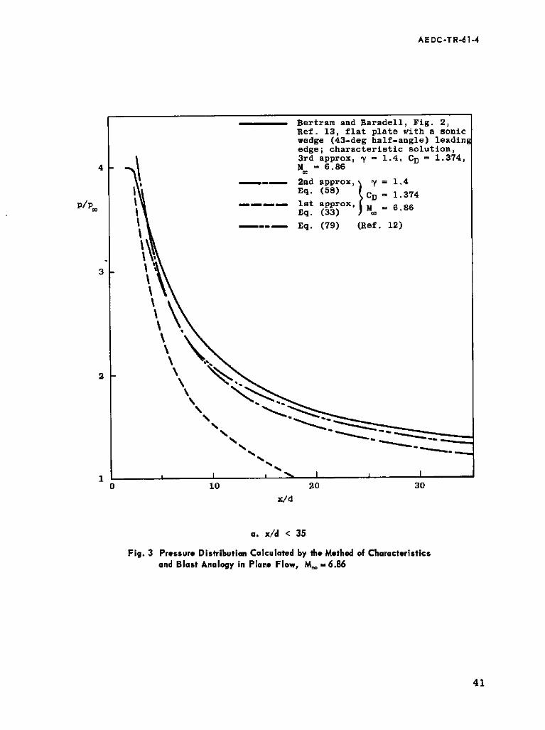
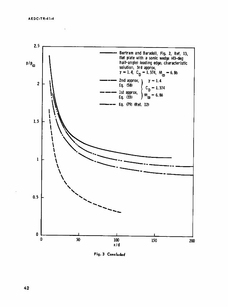
In Figs. 3, 4, and 5, approximations to the pressure distribution and shock shape in plane flow are compared with the theoretical results obtained from calculations using the method of characteristics.

The superiority of the second approximation to the pressure distri­bution at large x/d values for a configuration having a high nose drag is very evident at Moo = 6.86 from Figs. 3a and b. The difference between the theoretical and approximate pressure ratios at any given x/d is sub­stantially constant, and the approximate pressure ratio is within 20 per­cent of the theoretical value even at x/d = 150. A still better agreement, to within 10 percent, is obtained with the correlation formula, Eq. (79).

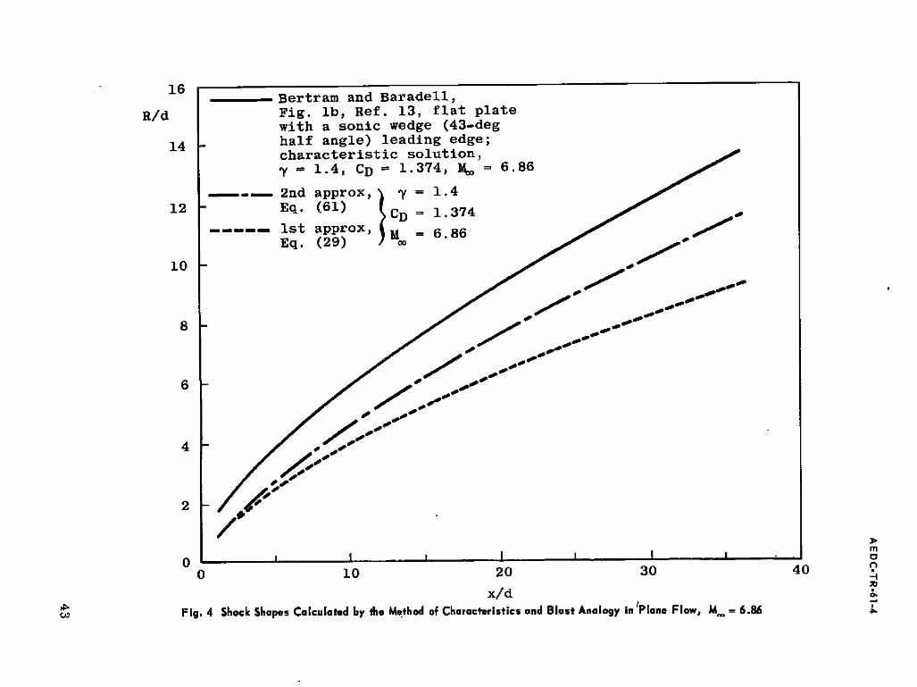
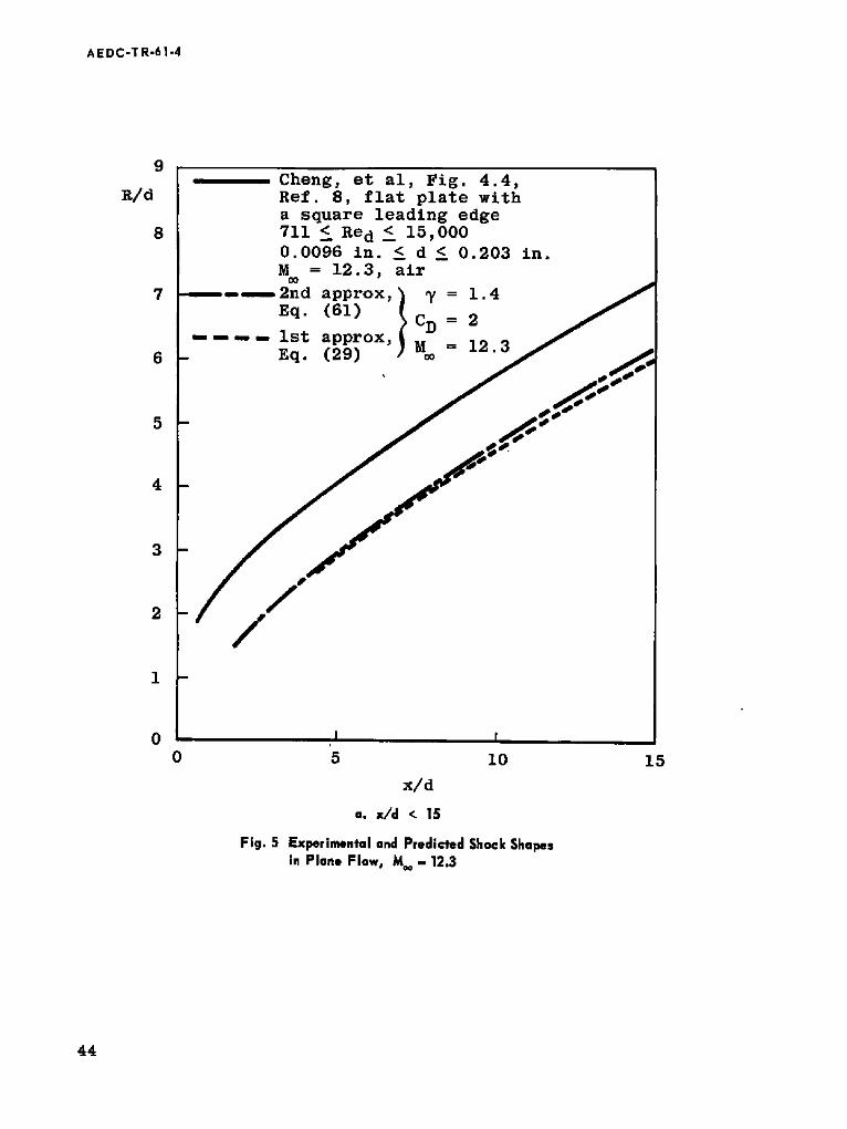
In Fig. 4, the corresponding theoretical and approximate shock shapes are shown, and the superiority of the second blast approximation is again evident. This is also the cas e at Moo = 12.3, Fig. 5; the second blast approximation gives values to better than 10 percent of the experi­mental observations.

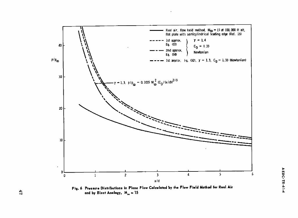
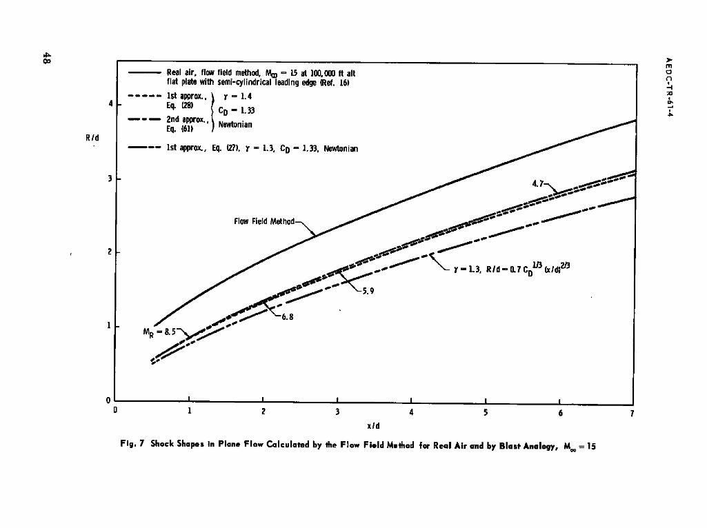
Results of flow field computations for real air obtained by the General Electric Company (Refs. 16 and 17) are shown in Figs. 6 and 7. The blast analogy does not predict the pressure distribution accurately for y = 1.4; a much better agreement was obtained for y = 1.3, Fig. 6. The shock slope, as in the previous cases, is well approximated by blast analogy for y = 1.4. In Fig. 7, the shock Mach numbers, MR, computed

30

AEDC·TR·61·4

from Eqs. (24) and (31), are shown and indicate that real gas effects might affect a significant portion of the flow field.

The data shown in Figs. 2 through 7 are plotted in terms of blast analogy correlation parameters in Figs. 8 and 9.

All theoretical results for pressure distribution, for y = 1.4, Fig. 8, correlate well with Eq. (79). The experimental data fall below the cor­relation of theoretical data. The inadequacy of the first blast approxi­mation is again clearly seen.

Figure 8 indicates that, although blast analogy provides suitable correlation parameters, the range of its applicability, in terms of x/d,

depends on values of CD and Moo' For example, with CD = 1.4, the pre­diction of pressure ratio becomes poor at Moo = 9.5 when (x/d) 2/3 / (M~ CD 2/3)

< 0.025 (x/d < 5), whereas at Moo = 20, it is good down to about 0.004(x/d '" 3).

Comparison of results of theoretical calculations for ideal (y = 1.4)

and real air, for Mach numbers of 20 and 15, respectively, presumably indicates the already noted significant real gas effects.

In Fig. 9, the available data on shock shape are plotted in terms of correlation parameters of the second approximation blast analogy, to­gether with the theoretical curve. The two sets of data correlate poorly. The experimental results agree well with the theoretical curve at large values of x/d.

From the above review of the limited data available for plane flow, it is apparent that blast analogy provides useful correlation of pressure distributions and shock shapes. Pressures are well predicted by the second blast analogy approximation for ideal gas, y = 1.4; results of a calculation for real air at Moo = 15 indicate pressures lower by 20 per­cent or more. Shock slopes are well predicted by the second blast analogy approximation, whereas the shock location shows an outward displacement relative to blast analogy prediction.

AXISYMMETRIC FLOW

Experimental Data

The available experimental pressure distributions on hemisphere cylinders at Mach numbers 6, 7.7, and 8 are compared with blast analogy and Love's (Ref. 11) predictions in Figs. lOa, b, and c. In all cases at x/d > 3, the second blast analogy approximation gives values much more

31

A ED C· T R·6 1·4

realistic than the first approximation and predicts the pressure distribu­tion accurately at Moo == 7.7 and 8. Love's method gives the pressure level accurately at- Moo = 6, x/d > 4, but is less accurate than the second blast analogy approximation at Moo = 8,

Pressure distribution on a flat-nose cylinder at Moo = 8 is shown in Fig. 11. Within the limited range of measurements (x/d :::;. 5.5), both first and second blast analogy approximations give an accurate estimate of the pressure on this high drag (CD = 1.64) body.

The experimental and blast analogy data on shock shapes are given in Fig. 12 for two of the cases already considered. As in the plane flow, the second approximation predicts closely the shock slope.

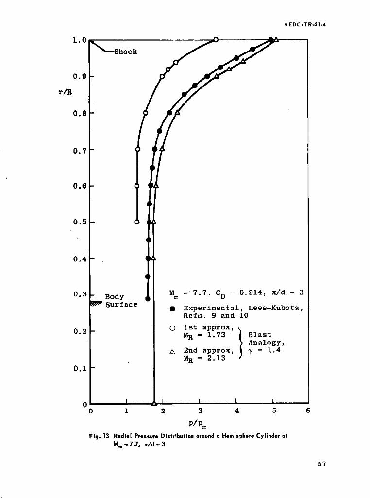
Lees and Kubota (Refs. 9 and 10) measured the radial pitot pres­sure distribution around the hemisphere-cylinder model at Moo = 7.7 at station x/d = 3 and computed the corresponding distributions of other quantities. These results for p/Poo and p/Poo are shown in Figs. 13 and 14 together with the corresponding blast analogy predictions. The latter were obtainedfromEqs. (3) and (8) with y = liMB. computedfromEqs. (24), (39), and (64).

The experimental pressure distribution, Fig. 13, shows an excellent agreement with the second blast approximation over the whole range of r/R. At the shock, the observed pressure ratio is 5, whereas the one computed from the second approximation blast analogy is 5. 13.

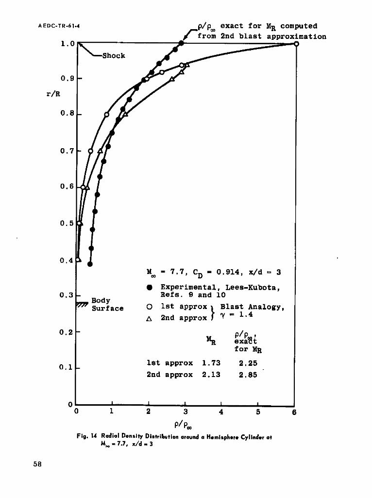
The density distributions are compared in Fig. 14. As mentioned previously, the second blast approximation gives the exact density ratio across the shock only at high shock Mach numbers. In this case, MR '" 2.13,

and hence a rather poor agreement is obtained with the experimental dis·­tribution. However, the exact p/Poo ratio for MR = 2.13 equals 2.85 and agrees well with the experimental value (Fig. 14).

Nevertheless, in view of the good agreement in the pressure distri­butions in Fig. 13, it can be considered that the flow field closely approxi­mates the second approximation blast solution. It is then possible to write, for the density distribution, an expression which is exact at the shock and to determine a function X' (K) from the experimental data, Thus, by analogy to Eq. (17),

(80)

(0) where h(K) is given by the first blast approximation and x' is computed to fit the experimental density distribution of Fig. 14. The values of x' are

32

A E DC· T R -6 1 ·4

given in Table 9 and were computed assuming MR = 2.11, which corre­sponds to the experimental pressure and density ratios across the shock. At higher shock Mach numbers, Eqs. (80) and (8) are in close agreement.

TABLE 9

VALUESOFX' (MR 2.11)

r/R 1 0.95 0.9 0.8 O. 7 0.6 0.5 0.4

X ,

5 1. 75 O. 1 -1. 45 -2.45 -3.2 -3.8 -4.25

Theoretical Data for y = 1.4

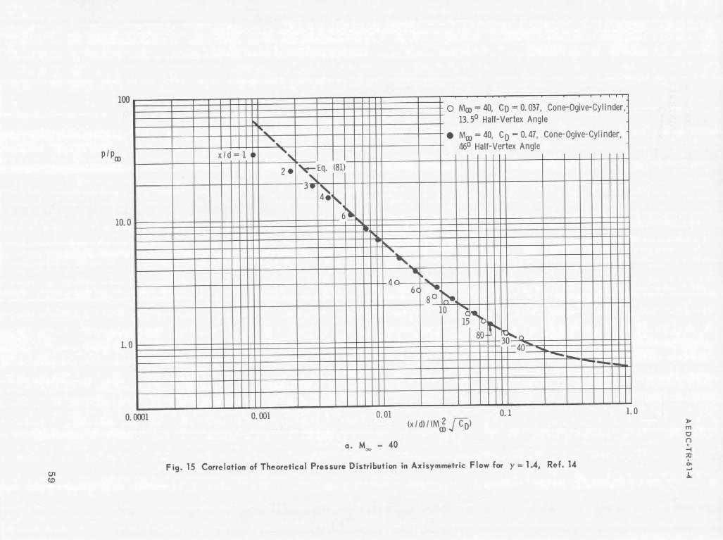
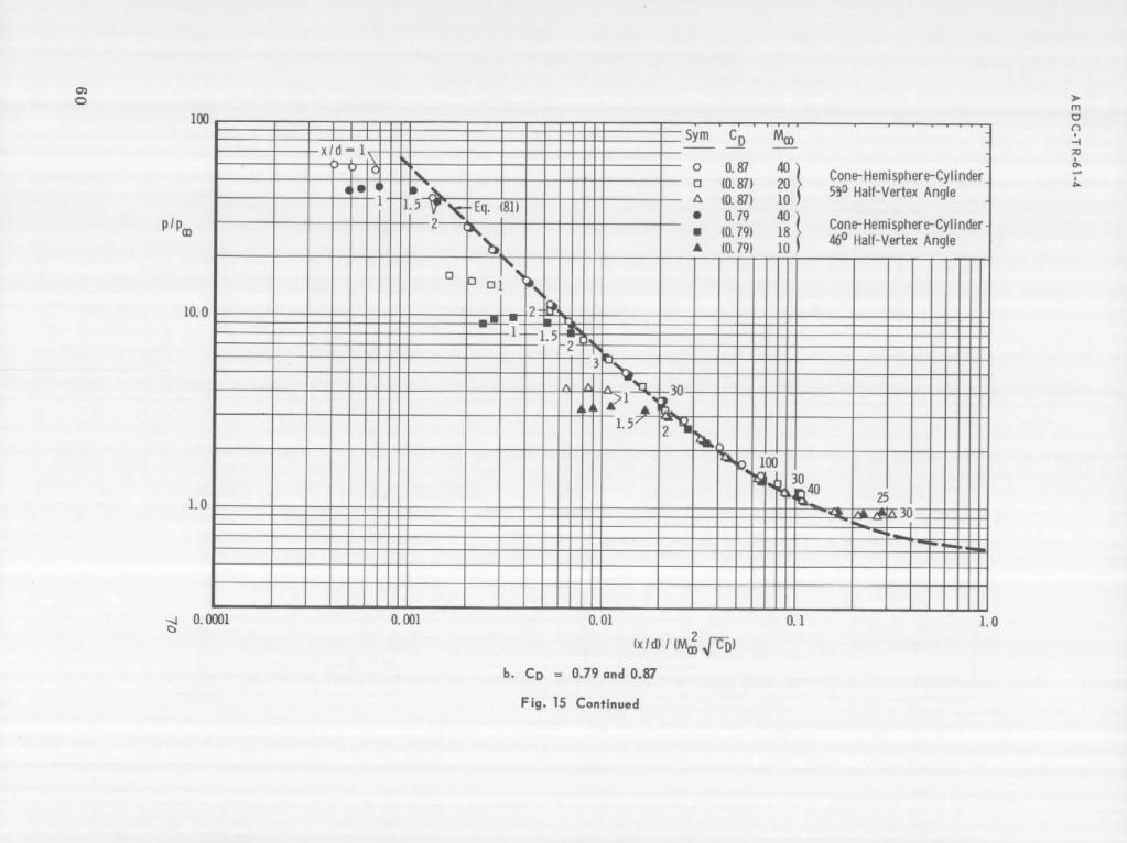
Van Rise (Ref. 14) published results of calculations of flow fields about cylinders with a variety of nose shapes, ranging in drag coefficients from 0.037 to 1. 37. Re used the method of characteristics to obtain sur­face pressure distributions and shock shapes in the flow of perfect gas with y = 1.4 and 5/3. In most cases, the nose drag coefficient was com­puted from the surface pressure distribution*.

Pressure distributions obtained by Van Rise are shown in Figs. 15a, b, and c in terms of the blast analogy correlation parameter, (x/d)/(M~ {C;;). Also in these figures is included the curve given by

p/Poo = 0.06 M':' Fn / (x/d) + 0.55 (81)

which was derived by Van Rise as representing the best correlation of all of his results for air (y = 1.4). Equation (81) above closely approxi­mates the theoretical blast analogy expression, Eq. (70) (see Fig. 24).

It is immediately apparent from Van Rise's results that the blast analogy provides an excellent means of correlating the pressure data over a wide range of drag and Mach numbers. It is also apparent that the range of validity of an expression such as Eq. (81) is limited, in each case, to a certain range of the correlation parameter. Based on Figs. 15b and c, for bodies with CD '" 1 and at Moo .::: 10, Eq. (81) predicts accurately

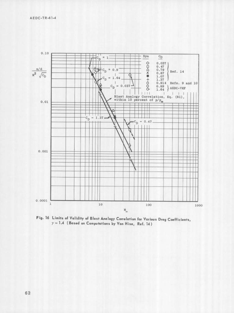
the pressure distribution at x/d .::: 2. The lower limits (in terms of free­stream Mach number and correlation parameter, (x/d) / (M':' Fo), of validity of blast analogy correlation are indicated in more detail in Fig. 16 for different drag coefficients, based on agreement in the pressure ratio to

~:<Values of CD assumed rather than computed are given in parentheses in Figs. 15 and 18. Only the results for y = 1.4 are here considered.

33

AEDC·TR·61·4

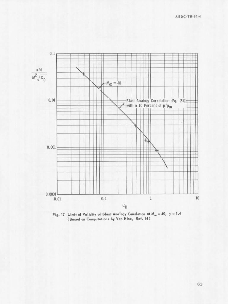
within 10 percent. The theoretical data of Van Hise is self-consistent, whereas the experimental data indicate higher limits of the correlation parameter for given Co and Moo' Similar data are presented in Fig. 17 for Moo = 40 and a wide range of CD'

As regards the upper limits of the validity of the correlation param­eter, the available data are not extensive enough to allow their determina:'" tiona In the majority of cases considered, good correlation was obtained for

In a number of cases in which calculations have been made into the region of plpoo < 1 (Figs. 15b and c, at Moo = 10 and 6.9), significant deviations from Eq. (81) are evident at plpoo < 1, but the data appear nevertheless to be well correlated by the blast analogy parameter. This, however, is not generally true, as indicated in Fig. 15c by the pressure distribution at Moo = 20, CD = 1.37, which deviates from other data already at plpoo '" 1.3

and at smaller p/poo values. As pointed out by Van Hise*, the results at plpoo < 1.3 may be subject to Significant cumulative errors.

The corresponding available results for the shock shape are shown in Fig. 18 in terms of the blast analogy correlation parameters. The correlation is good considering the wide range of drag and Mach numbers and falls slightly above the predicted CRI d) I (Moo Fn) values.

Theoretical Data for Real Air in Equilibrium

Two sets of theoretical calculations of flow fields around ahemisphere­cylinder in real air in equilibrium are available for comparison with blast analogy predictions and correlations. Feldman (Ref. 15) published results of characteristic calculations for Moo '" 18 (17,500 ft/sec) at 60, OOO-ft alti­tude, and the Gener'al Electric Company (GE) (Ref. 16) computed similar data for Moo '" 15 to 19 at 100,000 to 200,OOO-ft altitude, using the flow field method of Gravalos (Ref. 17). Details of tEe conditions for the GE calculations are given in Table 10 on the following page.

*Private communication.

34

A E DC-TR-61·4

TABLE 10

GE CALCULATIONS OF FLOW FIELDS AROUND A HEMSPHERE·CYLINDER IN REAL AIR IN EQUILIBRIUM

Uoo ' hoo' Poo , Poo X 106, Too'

M ft/ sec

CD ft lb/ft 2 slug/ft 3 oR 00

(15) 14,532 0.897 100, 000 23.085 32.114 418.79

18.24 20,000 0.914 150,000 3.0597 3.5642 500.11

18.1 20, 000 0.91 175,000 1. 2334 1. 4123 508.79

19.25 20,000 0.908 200,000 0.47151 0.6118 449.0

Shock shapes and pressure distributions obtained by Feldman(Ref. 15) and from blast analogy predictions (for y = 1.4, CD = 1) are shown in Fig. 19. As for the other data, the shock shape agrees well with the second blast approximation, except for a substantially constant, outward displacement of about (1/4) d.

The pressure distribution, as given by the second blast analogy ap­proximation, shows a fair agreement with theory at large x/d values.

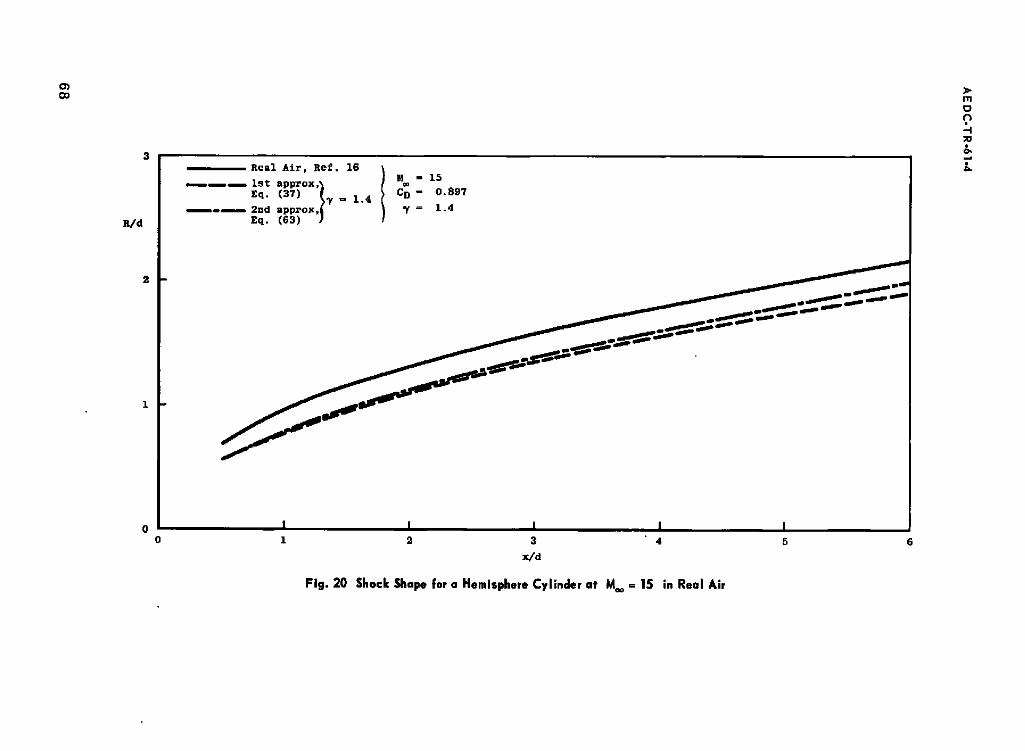
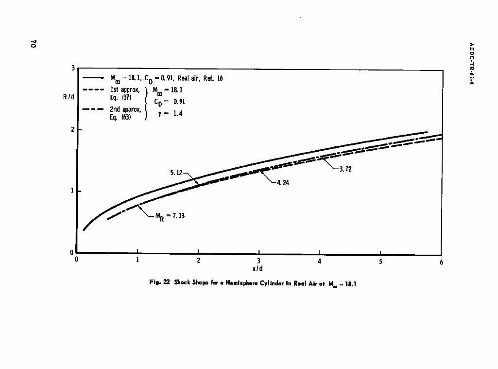
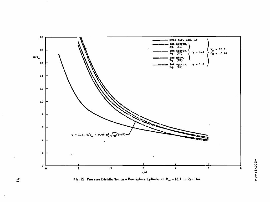
The GE data are shown in Figs. 20 through 23 for Moo = 15 and 18.1.

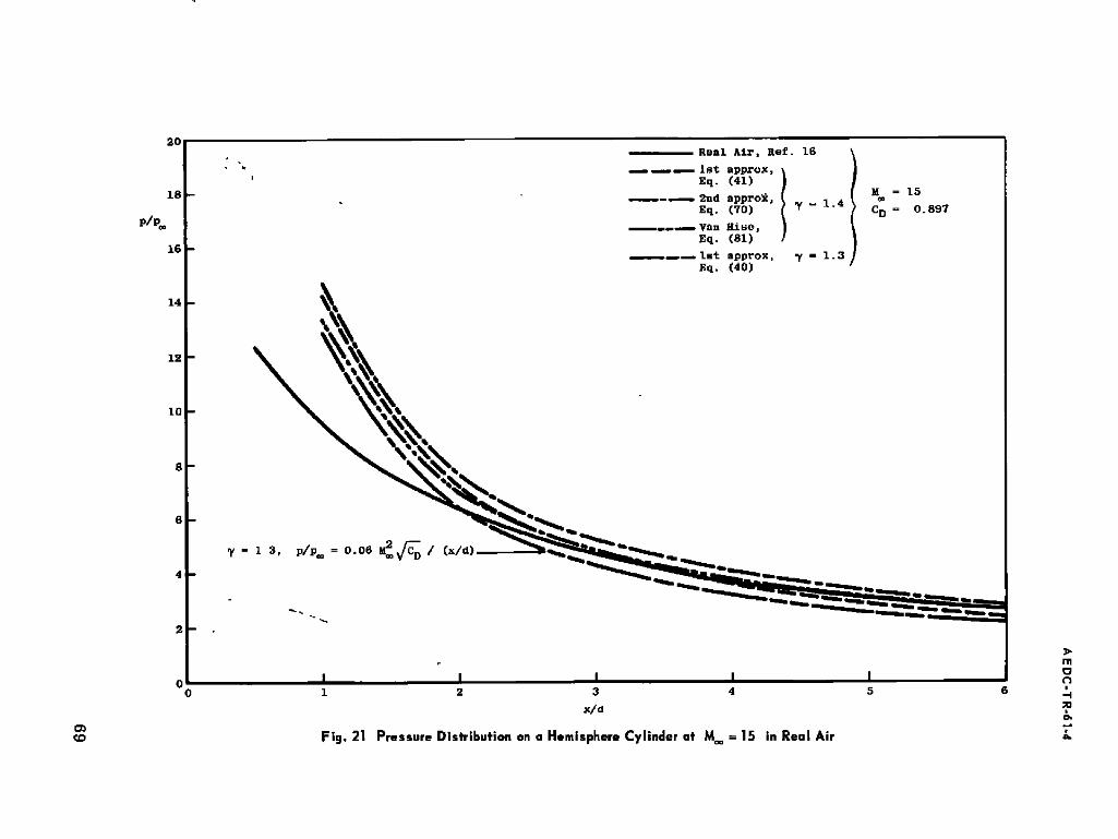
The shock shapes and, more particularly, the shock slopes are well pre­dicted. At Moo = 15 (Fig. 21), the pressure distribution agrees well with all blast analogy approximations for y = 1.4 at x/ d Z 3. At Moo = 18.1 (Fig. 23), the agreement is somewhat poorer at x/ d < 4, probably indicating a stronger influence of real gas effects. However, compared to the results obtained by Feldman (Fig. 19b), a much better agreement with the blast analogy is evident at small x/d values.

For comparison, results for y = 1.3 are also included in Figs. 21 and 23. It is apparent that a change in y does not account for the dif­ferences between the calculated and predicted pressure distributions.

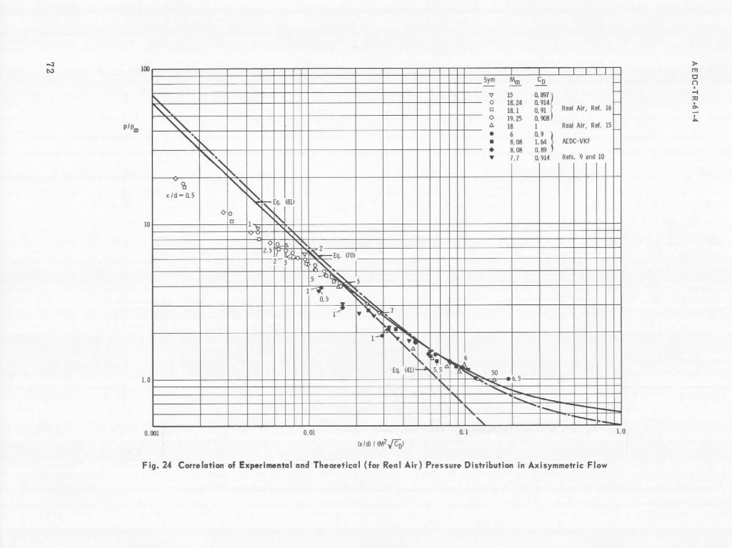
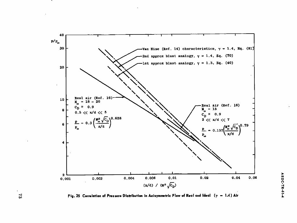
The real air data are shown in terms of the blast analogy parameters in Figs. 24, 25, and 26, together with the experimental results and curves representing blast analogy solutions and other correlations.

At lower values of the pressure ratio (Fig. 24) the real air results show a fair agreement with the other data. At pressure ratios above about 4, the real air results for Moo = 18 to 20 show a marked divergence from the blast analogy and the correlation of theoretical data for y = 1.4.

Also, unlike the theoretical computations for cone-cylinders and cone­sphere-cylinders (Fig. 15), the pressure distributions at lVl, = 18 to 20

in real air correlate well from the shoulder (x/d = 0.5) downstream.

35

A E DC· T R·6 1·4

These trends are more clearly shown in Fig. 25. It is evident that, whereas the Moo = 15 results in real air are in fair agreement with the y = 1.4 characteristic and blast analogy correlations, the Mx, = 18 to 20 data correlation shows a large change in slope, which cannot result from a simple change in the value of y.

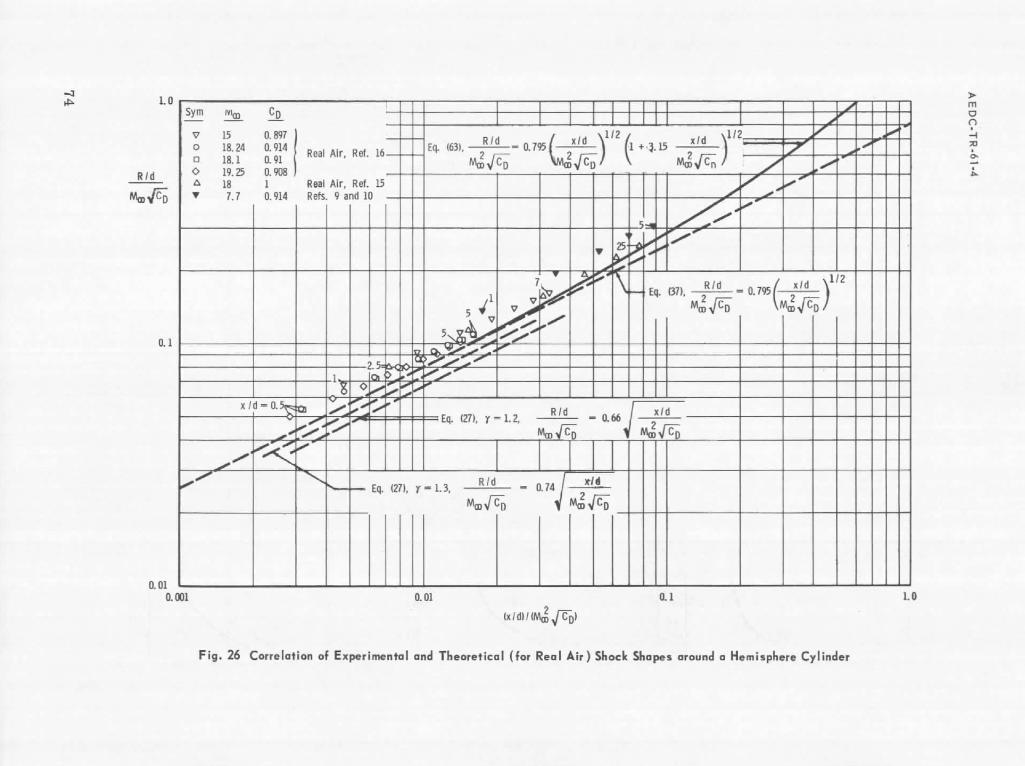
Shock shapes for real air are compared in Fig. 26 with the theoreti­cal blast analogy approximations (y = 1.4) and experimental data (y = 1.4).

At larger values of x/d [( x/d) / (M!, Fn) > 0.01], the real air results closely

approach the second approximation blast analogy prediction for y = 1.4. As indicated in Fig. 26, the agreement would be worse for y < 1.4. The only available experimental data fall above the blast analogy prediction, as already indicated (Fig. 12b). At small x/d values, smaller R/d values and smaller shock slope than predicted are found. This trend for real air coincides with results of the characteristic computations for y = 1.4 (Fig. 18).

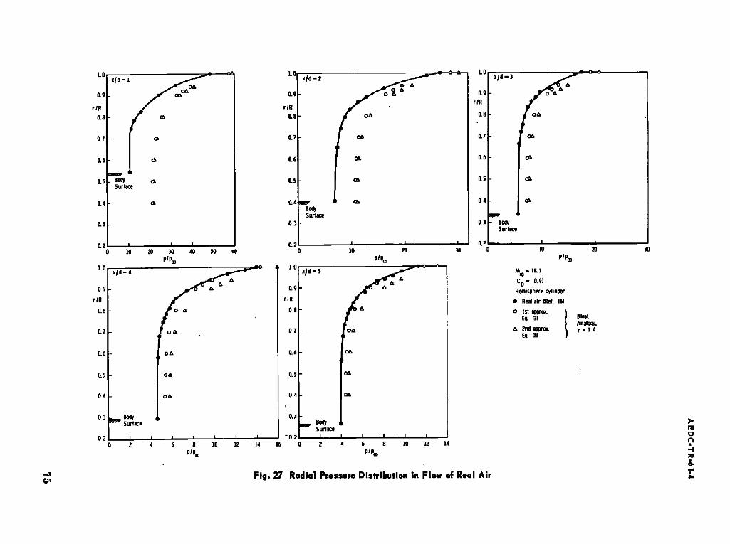
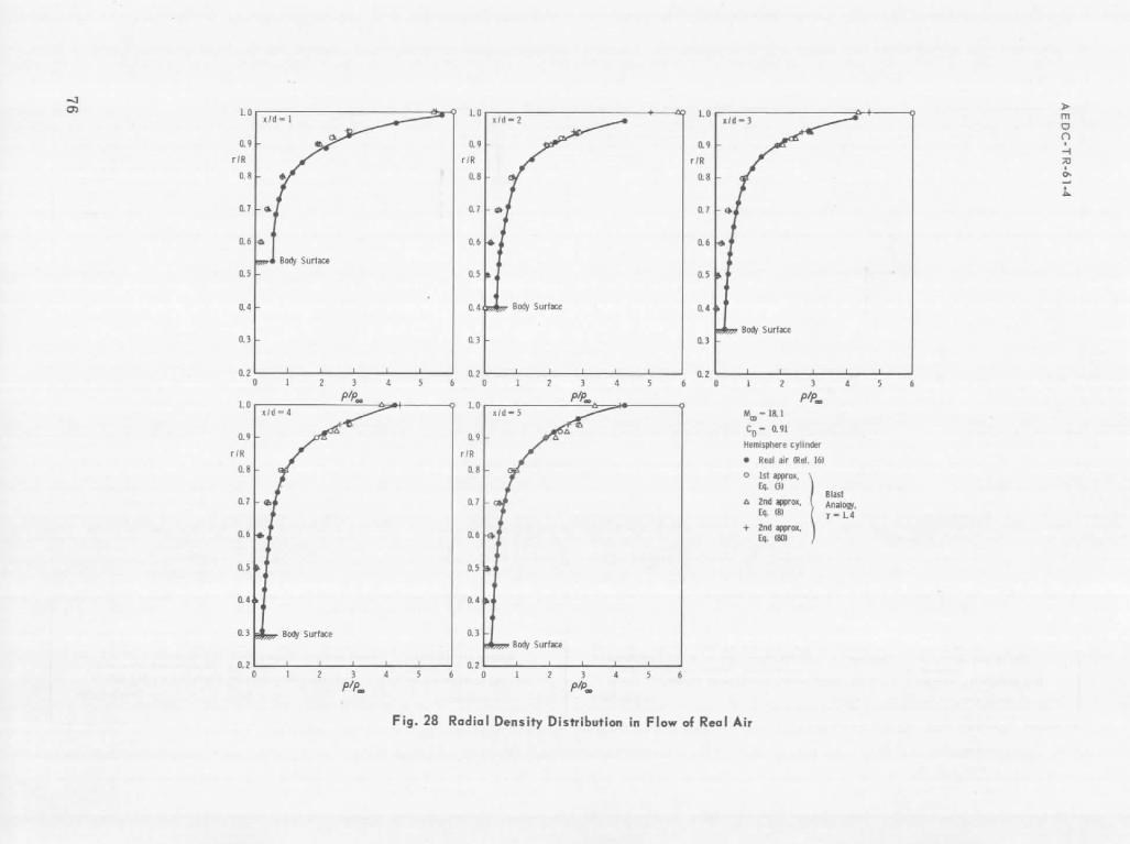
The radial pressure and density distributions computed by GE (Ref. 16) at Moo = 18.1 are compared with blast analogy predictions for y = 1.4 in Figs. 27 and 28.

As already observed, the pressure distribution (Fig. 27) is well pre­dicted at larger x/d values; in all cases, the first approximation agrees better with the theoretical results than the second approximation. This would be expected in view of the similarly better agreement in shock slope (Fig. 22).

The density distribution (Fig. 28) is in all cases well predicted at r/R > 0.8. At the shock, the second approximation gives more accurate values, and still closer ones are obtained using Eq. (80). At r/R < 0.8, the predicted density is much smaller than the computed one.

CONCLUDING REMARKS

Comparison of blast analogy (second approximation) solutions with correlations based on characteristic calculations for plane and axisym­metric flows shows good agreement between the two and thus provides a confirmation of the validity of the blast analogy method. The range of applicability of the blast analogy solutions depends on the values of param­eters (e. g., Moo and CD) which define the flow field; however, in general, at high Mach numbers and for ideal gas (y = 1.4), the blast analogy pre­dicts rather accurately the pressure distributions and shock shapes from

36

A EDC·TR·61.4

2 to 3 diameters downstream of the nos e to downstream stations at which the pressure has decayed to the free-stream value. Although the shock is displaced from the body more than predicted by blast analogy, the latter gives accurate values of shock slope.

As regards application of the blast analogy method to flow of real air, the available data are limited to semi-cylinder-plate and hemisphere­cylinder configurations at Moo '" 15 to 19, at altitudes from 60, 000 to 200, 000 ft. Comparisons indicate that blast analogy for y '" 1.4 predicts accurately the shock slope; the pressure distribution is predicted about as well as for experimental measurements made at lower Mach num­bers (6 to 8) and temperatures.

REFERENCES

1. Van Dyke, M. D. "Applications of Hypersonic Small-Disturbance Theory." Journal of the Aeronautical Sciences, Vol. 21, No.3, 1954, pp. 179-186.

2. Hayes, W. D. "On Hypersonic Similitude." Quarterly of Applied Mathematics, Vol. 5, No.1, April 1947, pp. 105-106.

3. Taylor, G. 1. "The Formation of a Blast Wave by a Very Intense Explosion." Proceedings of Royal Society (A). Vol. 201, No. 1065, March 22, 1950, pp. 159-186.

4. Sakurai, A. "On the Propagation and Structure of the Blast Wave, 1. " Journal of the Phys ical Society of Japan, Vol. 8, No.5, September-October 1953, p. 662.

5. Sakurai, A. "On the Propagation and Structure of a Blast Wave, II. " Journal of the Physical Society of Japan, Vol. 9, No.2, March-April 1954, p. 256.

6. Lin, S. C. "Cylindrical Shock Waves Produced by Instantaneous Energy Release." Journal of Applied Physics, Vol. 25, No.1, January 1954, pp. 54-57.

7. Cheng, H. K. and Pallone, A. J. "Inviscid Leading-Edge Effect in Hypersonic Flow." Journal of the Aeronautical Sciences, Vol. 23, No.7, July 1956, pp. 700-702.

8. Cheng, H. K., Hall, J. G., Golian, T. C., and Hertzberg, A. "Boundary-Layer Displacement and Leading-Edge Bluntness Effects in High Temperature Hypersonic Flow." Institute of the Aeronautical Sciences Paper No. 60-38, January 1960.

37

AEDC-TR-61-4

9. Lees, Lester and Kubota, Toshi. "Inviscid Hypersonic Flow over Blunt-Nosed Slender Bodies." Journal of the Aeronautical Sciences, Vol. 24, No.3, Mal'ch 1957, pp. 195-202.

10. Kubota, Toshi. "Investigation of Flow Around Simple Bodies in Hypersonic Flow." Guggenheim Aeronautical Lab., Calif. Inst. of Technology, Hypersonic Research Project Memo No. 40, June 25, 1957.

11. Love, E. S. "Prediction of Inviscid Induced Pressures from Round Leading Edge Blunting at Hypersonic Speeds." ARS Journal, Vol. 29, October 1959, pp. 792-794.

12. Baradell, D. L. and Bertram, M. H. "The Blunt Plate in Hyper­sonic Flow." NASA TN D-408, October 1960.

13. Bertram, M. H. and Baradell, D. L. "A Note on the Sonic-Wedge Leading-Edge Approximation in Hypersonic Flow." Journal of the Aeronautical Sciences, Vol. 24, No.8, August 1957, pp. 627-629.

14. Van Hise, Vernon. i'Analytic Study of Induced Pressure on Long Bodies of Revolution with Varying Nose Bluntness at Hyper­sonic Speeds." NASA-TR-R-78, 1960.

15. Feldman, S. "A Numerical Comparison Between Exact and Approxi­mate Theories of Hypersonic Inviscid Flow Past Slender Blunt­Nosed Bodies." A VCO-Everett Research Laboratory, Research Report 71, June 1959, also ARS Journal, May 1960, pp. 463-468.

16. General Electric Company. Private Communications, November 1960-February 1961.

17. Gravalos, F. G., Edelfelt, 1. H., and Emmons, H. W. "The Super­sonic Flow About a Blunt Body of Revolution for Gases in Chemical Equilibrium." Missile and Space Vehicle Department, General Electric Company, GE-R58-SD-245, June 1958.

38

AEOC-TR-61o4

0 .7

A

=,80. 6 _

v

0 .56 - - - - - I

~ 8 0 5 _ ~ •

0 . 4 0 . 6

I I I [ 0 . 8 1

Plane, a = 0

i I i 2 3 4

( p / p = ) "

I I I i i i

5 6 7 8 9 1 0

0 . 7

0 . 6

i 0 . 5 -

~ 0 . 4 4

0 . 4 -

0 . 3

A x i s y m m e t r i c , ~ = 1

t ~ i I i I I I

0 . 5 1 2 3 4 ( p / p = ) "

P

O. 395 : f o r ( p / p = ) ~ o=

I I I i l

5 6 ? 8 9 1 0

Fig. 1 Comparison of Pressure Ratios as Given by the First and Second Blast Analogy Approximations at a Given x/d Station (y = 1.4)

39

AE

DC

-TR

-61-4

0

P4

0

r=g ,,=I 4

J

.0

• "

4=) ~u

~ u

• ,'4 0

I=

~P II

• ~.,.q

-

~ r,.

'0

Gi

~ ~

r,- -

• ,o~ .o

~ o'

- o"

-.~r-g

~

0 0

~) 0

~,~

•

...,, ,.,

I "~

~; I1

• '

Jl '!+ ! ,I

I

r •

-/

I r

I I

I I

I I

I o

~8

o O~

t",.

u~

II 8

)- 0

U=

(11,

0,.

o~

0

.i

.m

a E m

.o a,. "12

._u "U

o,. "0

I)

C

0 E 0 L.

X U

J

iN !

._m

U=

40

A E D C - T R - 6 1 - 4

P/P==

3

2

1

l l

0

,\ l l

\ \ \ \ \ \

% %

% %

I i ~ I I I0 20

x/d

Bertram and Barade11, Fig. 2, Ref. 13, flat plate with a sonic wedge (43-dee half-angle) leadin edge; characteristic solution, 3rd approx, T = 1.4, C D = 1.374, M = 6 . 8 6 0¢ 2nd a p p r o x , ~ 7 = 1 .4 Eq. (58) I C D = 1 .374 1 s t a p p r o x , Zq. ( 3 3 ) M = 6 . 8 6

Eq. (79) (Ref . Z2)

I 3O

a. x/d < 35

Fig. 3 Pressure Distribution Calculated by the Method of Characteristics and Blast Analogy in Plane Flaw, M~o = 6.86

4 1

AEDC-TR-61-4

2.P

p/p®

2

1.5

]

0.5

Bertram and Baradell, Fig. 2, Ref. ].3, flat plate with a sonic wedge (43-deg half-angle) leading edge; characteristic solution, 3rd approx, i' = 1.4, C D = l. 374, M m = 6. 80

~ . m 2nd approx, )' = 1.4

/ ~ Eq. ( 5 8 ) CD=1.374 I.~\ - - - ~I ~,~;ox, ~°=~.~

\ \

\ \

Q - - D

- - m - -

50 I

I(B xld

150

Fig. 3 Concluded

200

42

AED

C-TR

-61-4

0

IQ

!

~ ~

..

..

X

X

~

U

'cI -

~.,-I

0 ff'J

il II

II X

• ~-

"~

1:13 •

~ .~4

II "

X ~

,

q..4

.-,/=

bn.,~ ,-4

os II

"{3 ._

~ -.

~ ~

I !

\ ~ -

1 I

I I

I I

I "q" .m

~ C

q 0

00 r~O

~

0,1 0

u. r'-I

r--I r-'l

r-I

43

AEDC-T R-61-4

9

R / d

8

7

6

5

4

3

0

C h e n g , e t a l , F i g . 4 . 4 , R e f . 8 , f l a t p l a t e w i t h a s q u a r e l e a d i n g e d g e 711 < Re d <__ 1 5 , 0 0 0 0 . 0 0 9 6 i n . < d < 0 . 2 0 3 i n . M = 12.3, air-

--9-------2nd approx,~ T = 1.4

,..q. ( 61 ) ~,cD -- 2 --------ist approx,~, - 1,~ ~ ~ / "

_ Eq. ( 2 9 ) , , , -*oo - " " . ~ , / .,,~,-I

/ / /

0

I I

5 10

x / d

a. x/d ~. 15

Fig. 5 Experimental and Predicted Shock Shapes in Plane Flow, M - 12.3

15

44

AE

DC

-TR-61-4

...,.~

• ,,~1

fl,)

"0 •

fl.) fl)

~

• ,.,,4 ~ l:d~O

~...i ~-,.I

~ -

I~,,~ .,-I Lt~

~,.~ .4..~ "~ ~'1

~v

!

r..i r-.,I

.',~0

IlJ ~.1

,\ ',,,, ~\., \ \

.r'l

0 vl "0

,r-I

vl~

~ -r.I

~,D 'r,-I ~vE= Q

II

,-i ~8

II II

II

0 0

l'~ "~4 ~

1"~

'

I i

i I

I ' I

I L~ r"'l

\ ,,,,,

Q

I LO

Q L~

-- Q

O 0

0

0

"0 ,,o v

0 =11 []

0 U om

Ii.

45

AE DC-TR-61-4

80

R/d

70

60

50

40

30

20

i0

0 1 0

Cheng, et al, Fig. 4.4, Ref. 8, flat plate with a square leading edge 711 ~ Re d ~ 15,000 0.0096 in. < d < 0.203 in. M = 12.3, ~ir --

2nd approx,~ 7 = 1.4

Eq. (61) ~C D 2 1st approx,|~, Eq. (29) ) " ~ 1 2 . 3

J

o ~ ~ ° ° ~

J

100 I I

300 200

x / d

c. x / d . < 400

Fig. 5 Concluded

400

46

A ED

C-T

R-61.4

!/ .

_ t

='-' .~

"~

~ It l/

: ~

~'° ~

lift l

.,

~.

~

,~

.~: ~

~ ~

., ;'

•,

I '

I !

~ "'

o I

! ~

~/ ,

E

. ° r ~

if, it.

I

N

N

o

o

"~

8

4"1

AE

D

C-T

R-6

1-4

......

a

,..®

"*

~ g

I' i

I , I

| J

I I

r~

. *O

,q.

m

~J

O

O

U~

II 8

m

O

m a m

2 m

.Q

D

h ,m

IJ iv o ID

-a

IJL.

O

u.

o

=Q

_o

U

o U

o L

I.

o o Q

. P

m

&

D

.G

V)

U

O

..G

m

U.

48

s

A E

DC

-TR

-61

-4

O

o E .I= O

D

. >

,.

8'

I¢ .<

O

-10

o U O

u.

o

"8 G

.

.P. II)

°~

r~

D

I/t .o

n GO

M.

4g

AE

DC

-TR

-61

-4

0

U

0

0 ~8

x

i.

O

E 2 U

a.

u O

E~

O

i m

J O

O

U O

w.

O

E~ O

a. C

0 a.

o

ill u o

Ill m

.i li.

50

AE

DC

-TR

-61

-4

""

I

: e

~

~ I

"0 m

c~

I I

I:: -~

~

I • ~

- ~l

• o

I ,-f e,j~

0 k

~l

~ m

g

~

::SO

P

~

•

•

a ~

m.,-,

,,,.., .

• ®

,-.~

,~

o~ ~

I I

8~

•

" ~

=

.~

,~

o

~ •

J I

Q}

.,-I I~

.,..i ~

I '

C~

O

'~

0 ~

~ ~

l 8

" I

• ,~

,~

0 ~

-~

r~

:II

I I

El

I~ "--" ~ "~

~

-- ~

. I

-=

= oo

o o

• I

I r~

•

• •

~,

~

B~

- I

g H

II

~v

~',,~

" "

I I

." I

• I

I I

~ ~

.~..,.,.

~..

, ,

.

~ c

q~

,.~

~

[ ,

,

• I

I P

: U

I /

~ l

n m

//

o

,, e/

/ /

/I /

I cq

I .-I

°.

z 0 U

| o

.Q

0

51

AE

DC

-TR

-6 I-4

fl

.if.. ~- ~, ~,,

• j

,_.

.._,~

~

>" <,@

~ ~

T..,.,.4

E

,"-I C

.l" x =

l ..o II

,~"

mM

.-~ g

g g

l~ll I,i.~"

~,-I li,l.,I

!

'' /

I I

,

I

i #

11 #

/, # # "

#

. i I

I

I'.~, t i

S

S S

I |

L I

~o

il.

O

52

A ED

C-TR

-61-4

,.- E

II

.~

s -

/ •

i I J

~

/.." i

o/

/';/

J i ,r

I I

, I

0

w

x ~.

U

0

d '-

~ m

o~

° U

.

53

AE

DC

-TR

-61

-4

tO

~0

~

.~

• ~ "0

~0

~

0

~0

~

~0~

~ ~.~

~LO

~ ~

~ 0~-~

O~

~

~ ~

4-~ +~ ~,0

~.~

I ~

o0

om

'o ~-~ O

~e-~

~.~

0

mN

o ~o

~0

~

~ .~

II II

I ~

O

"~' ~

0 ~

II

II 11

I]

oo 0

0

II m

~.~ ~

~,"

I J, n

! I I,

lj1~

"/"

.,,' .,,,"11

l,,,,~"v

,, ~ S

II

L,,, S

t I !

Im I

/..,,,

', / /,/ u

I

/,',I / I

," IIiii I

m

o,

I I

q3

m

m

I n

i-

n 0

0

~0

tO

"0

Oq

i-.I

n 8

3E

0 "ql

U 0

S Z 4~

u 11_ g c 0

I m

L

.u

L c [] 0 .e

i N ILl

L

54

AE

DC

-TR

-61

-4

\

\ \ \ "0

or,I \'

~4 ~o

o ~

u u

II \

o o

%

• ~ .o

,~

~c

~

~.

~,

II ~1

~ ~1 ~-~

~1

~

I 0

U

I I I I I

O

i-I

1.4

(3")

00

L',-

C~

c

"O

n

3E

"O

.E

U Q

L D1

"r: Q

-12

l~

o EJ

a.

O

J~

U

O

j-

"12

._u

L "u

c D []

O

E o

--

D.

K

IAi

in o

O1J

o~

IL

55

A E

DC

-TR

-61*4

. ~

'1:1 ~

II II

H

0,-I

II N~

\ \

I

I •

r~ II

II II

o~ .,-i

-I-

a~

I

O

O

c~r.d ,~

r.d

I s I

I I

I' I I I

+ \-

++.\,\

÷-4- I

"/'÷./..,. O

O

i--I

00

~D

O'J

P=l

O

=u o u

8 U o~ li.

56

1 . 0 ~ S h o c k

AEDC-TR-61-4

0 . 9

r / R

0 . 8

0 . 7

0 . 6

0 . 5

0 . 4

0 . 3

0 . 2

0 . 1

0

- Body ~ S u r f a c e

M~ = 7 . 7 , C D = 0 . 9 1 4 , x / d = 3

E x p e r i m e u t a l , L e e s - K u b o t a , R e f s . 9 and 10

O 1 s t a p p r o x , \ M R = 1 . 7 3 I B l a s t

A n a l o g y , A 2nd a p p r o x , ~ = 1 . 4

M R = 2 . 1 3

~ 1 I i I 0 1 2 3 4 5

p/p Fig. 13 Radial Pressure Distribution around a Hemisphere Cylinder at

iVl .7.7, x/d~-3

6

5?

A EDC-TR-61-4

I . 0 ~ ~ ~ S h o c k

0 . 9 .

r/R

f p / p ~ e x a c t f o r M R computed f rom 2nd b l a s t a p p r o x i m a t i o n

0 . 8

0 . 7

0 . 6

0 . 5

0 . 4

0 . 3

0 . 2

0 . 1

0

f B

Body ~ F / S u r f a c e

M = 7 . 7 , C D = 0 . 9 1 4 , x / d = 3

• E x p e r i m e n t a l , L e e s - K u b o t a , R e f s . 9 and 10

O 1 s t a p p r o x } B l a s t A n a l o g y , 2nd a p p r o x 7 = 1 . 4

p/p.,,, MR e x a ~ t

f o r M R

1 s t a p p r o x 1 . 7 3 2 . 2 5

2nd a p p r o x 2 . 1 3 2 . 8 5

I I I I I 0 1 2 3 4 5

P/Poo Fig. 14 Radial Density Distribution around a Hemisphere Cylinder at

M~o - 7 .7 , x / d .. 3

58

8 o

.

C~

C~

AE

DC

-TR

-6 I-4

s-=

O II

O

14.

N

8 E E

v

C

o~

O

,0=

°-- °

r~ U

n U

°- =

I- O

O

O

o~

U c~

o~

u

.

C~

59

AE

DC

-T R

-61-4

80

8 0.

c~

,--e

0

x

d 7~

c~ -o @

o '~. C

h

0

c~ u

II U

') p

.

U

,.

8 C

2=

C2=

0 c5 0

A E

D C

-T R

-6 I-4

0 0

o _

d v

0

qO

"" II

x ,-.

,', ~,

I J- L;

0==e

c5

d

61

AEDC-TR-61-4

0.10

x / d

0.01

O. 001

O. 0001 i

Fig. 16

| . 9

I • 64

i I - 0 . 0 3 7 ~

I I I-

I Sym

O O

X

!

J i l l

CD

0 .037 0 .47 0 . 7 9 0 .87 R e f . 14 1 .07 1 .37 0 . 9 1 4 R e f s . 9 and 10 0 . 8 9 } 1 .64 AEDC-YI~

I I [ [ l i t B l a s t Ana logy C o r r e l a t i o n , Eq. ~ i t h t n 10 p e r c e n t o f P/Pm

~ m

- - - - 4 - - - ~ - -

~ C D - 0 .47

k

---NC- ------e~_ ~

b I -j I

,

(81),

I0 i00

Limits of Validity of Blast Analogy Correlation for Various Drag Coefficients, y ,: 1.4 (Based on Computations by Van Hise, Ref. 14)

I000

62

A EDC-TR-61-4

0.1

x/d

0.01

0.001

O. 0001 O. Ol

Fig. 17

0. I 1

C D

Limit of Validity of Blast Analogy Correlation at Mo~ = 40, (Based on Computations by Van Hise, Ref. 14)

y = 1.4

10

63

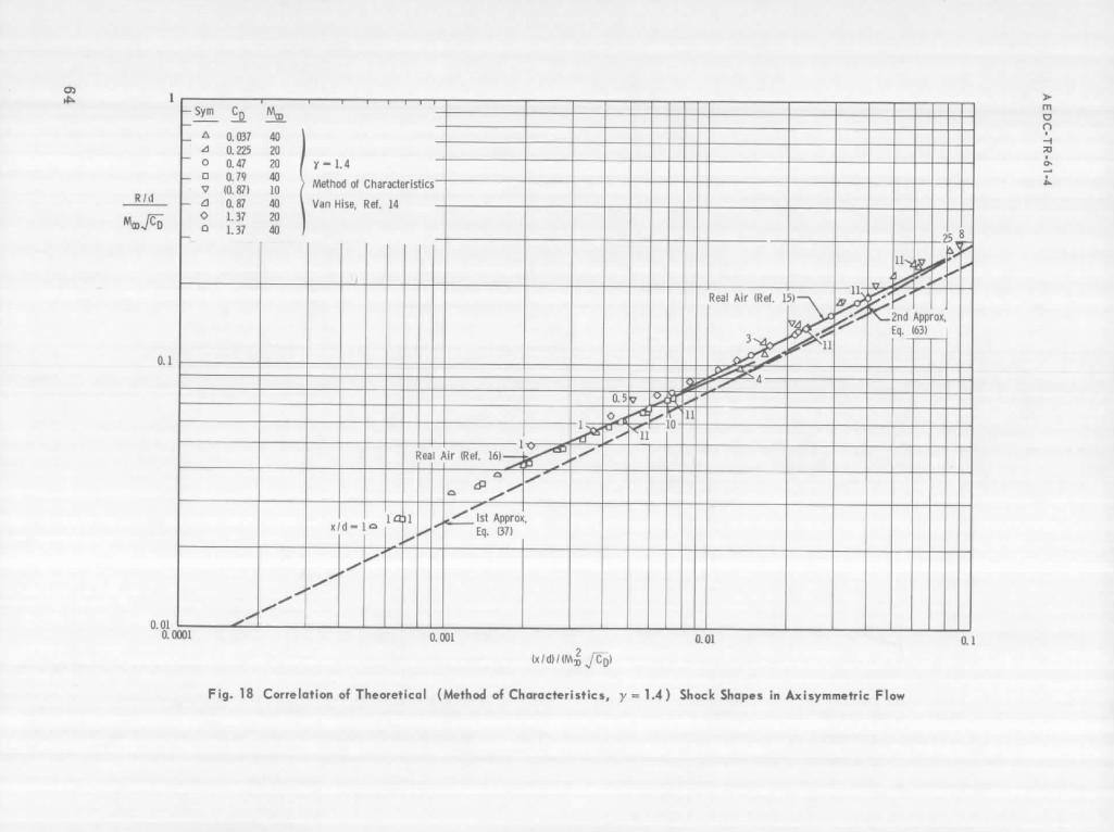
A E

DC

-TR

-6

Io4

.~- o

I

~N

oo

Dq

oo

64

,B

\ \

\ \

O

d

O

14. U

o

~

o E E el

o~

@

O

,4=

U

O

I-

A II

._u

~F~ "~

E O

,=C

U

"S

"8 @

3E ~

=~

U

oD

4

- O

o ,=

~

I- O

°~

4-

O

U

CO

o~

ii

AE

DC

-TR-61-4

U~

\ \ \ \ \

~ 00

~ II

II H

u'J I::t

~ ,,-I .,-t

GS .I-4 ..~ ,-f

f..,

I r.)

OS ~ U}

~.~,~ 0

- c~'¢ ~'¢ ~

"~

~ "~

' S

~,t~ ~34L ~,

c~ ~

4'0

•

C3 0

~34~0 ~34c,3

,-i ~.~

"0

• +~

•

I 1

, !

I, I

,'\ I

I I

I. ,~

o'3

04 ,-I

i ]

~ 8

-i i ~.

0 .~

._u

in ~

"12

a ~

g g

,.~

4,. U

0

U

U'S

CO

Q

o,

o _~ ilk

65

AE

DC

-TR

-61

-4

O

O0

i-4

- I ~

.~1

,,,~

f.l ~=I f., .i-I .~

• O

U

OO

~.~

~I ,~

~D ~

II U

II

O

O I

I ,

I I I

I,

I i

I I

I I

00 ~D

/j /J I

/ I

/, I . I

O

C~

O

LN

I - O

O

O

O v!

~°

U

1: w

O

~

I

IA

ui

n .d

66

A EDC-TR-61-4

p/p®

100.0

10.0

1 . 0

0 . 1 0

F e l d m a n , R e f . 15 , hemisphere-cylinder, m e t h o d o f c h a r a c t e r - i s t i c s , real air, 60,000 ft altitude, 17,500 ft/sec, M = 18

2nd approx,~ T = 1.4

Eq. (70 ) I C D - i I s t a p p r o x , Eq. ( 4 1 ) M~ - 18

10 20 30 40

x / d

c. Pressure Distributions, x/d < 50

Fig. 19 Concluded

50 60

67

AE

DC

-TR

-61-4

u~ 0

i-I i-I

D I

II

~ 8 r,.~

2'-

r-I n

H

X

- 0

0

r4 tl

I ,

tl

'13

68

I. O

R

,<

"4 0 e

~

i: =

i

u~

it 8 =E

"13

i 2 0 j- Q

. tQ

im

E Q

:C

0

t4.

0 D.

i cq

0 J=

V

) u 0 J~

t~

0 rd

u.

0

0

A E

DC

-TR

I61

-4

0'1

u'l 0

g II

] II

iii

,,~ ~

,~

eL~,,.

.,,~ ~ ~

.,~

M

I !'

, il

If

0 II I

f t

I I

I I

I I

I I

I

~8 eu

O

b o

i O

C

°~ il 8

C

U .o O

O

@

O

D

..Q

.i a D

L e

IL

69

A E D C-T

R-61-4

O~

g II

il

g

II ~'~----

m

f"-,i l.h

l l=

%lW

i i

I I I

I l

I

ep

.

I',,,,,. N

i=-i

u~ i=,=i

II

X

N

ilC~

,

0

n I0

Ii u

i 0 [] li

.==

U 0 j. 0 Z I0

11 &

O

.J=

U

@

J~

(N

li IL

?0

AE

DC

-TR

-61

-4

• •

00 O

P

.l

I II

,,8 ~

eiv

I~I ~=. '

r=l

l:d ,"il~

0111~

I~N

,=

~N

fill

vi l

%8 ~D

O

O fl

w-I

fl

I I

I I

I I

I I

I O

00

CO

~

I' k'q

O

a0 S

D

q'

cq

Cq

,,=I ,=.I

,=4 ,,=I

1,4 ~e

- C

q

O

O

O

iv

GO

II

~E

,=~

iS

m

m

U

,=C

Q.

"E O

Z U

O

O

Im

4.= D

#i

Im

.e IB

G=

U.

71

AE

DC

-TR

-61

*4

E

I I>

oa

O

~

• I

O1

~

T2

L~ ~

d I x

o

O

LL

U

o~

@

E E Lq

c~ *m

F" O

*m

°~

U~

a.

.m

m U U

m

J ! -i X

Ill

J U

L~I

,m

LL.

A E

DC

-TR

-61

-4

o

i• i

i I

I i

I I

I I

.,

-~

~

~I.~I , .

,, "

" ~

v ~

/ •

• ~"

V L',-

s.

f.d ~

~ •

"o ,M

//

{~ -

- 0d

,--I ~4

0 //

+~ ,~

H el

V .

//

m

•

8 ~

1 8

.// • "4

II li

=~

U

¢~

~1

~,

//

.~(/ 7

/ I

,~

o ~,~ ~

• ~I

o. ~

I I

I I

I I

I I

I

o o

o Q

0 ,.,G

~IP

c~4 ....i

o

II

.b

'=o

"S

| Ul

J~

o

E O

= "S

o • 4,=

E U

o o

¢~I o

?3

AE

DC

-TR

-61-4

o

1',t

o

p.e O

)<

"O

°-

U .o

O

.¢ el

"i

-t-

o "O

l¢

o ¢1 f/I

& U

.¢

.ld

O

..¢

,< O

n/

.u_

O

..¢

I- "O

¢-

D

C

O

E °~

O.

)<

ILl

I¢

O

~N

,e-

(J

¢'4

O)

ii

AE

DC

-TR-61-4

4d d I

I I

I I

I

?

8 6

,, !:!,

I I

, , |~

d

i i

.~r

L~

O R 2

8 l

i i

i i

I I

o I

I I

I I

t,=

0 0

I I

,|

m~

|

h .m

O

Q

~"

. IJl=

..=

. J 2 m

Q

"13 o

•

o

D.

,o

¢.~

7.5

AE

DC

-TR

-6 I-4

÷

! ._~

78