Embed Size (px)
Citation preview
Arithmetic RandonneeAn introduction to probabilistic number theory
E. Kowalski
Version of June 4, [email protected]
“Les probabilites et la theorie analytique des nombres, c’est la meme chose”,Y. Guivarc’h, Rennes, July 2017.
Contents
Chapter 1. Introduction 11.1. Presentation 11.2. Integers in arithmetic progressions 11.3. Further topics 71.4. Outline of the book 91.5. What we do not talk about 9Prerequisites and notation 10
Chapter 2. The Erdos-Kac principle 122.1. The basic Erdos-Kac Theorem 122.2. Generalizations 162.3. Convergence without renormalization 182.4. Further reading 21
Chapter 3. The distribution of values of the Riemann zeta function 223.1. Introduction 223.2. The Bohr-Jessen-Bagchi theorems 243.3. The support of Bagchi’s measure 343.4. Selberg’s theorem 373.5. Dirichlet polynomial approximation 443.6. Euler product approximation 463.7. Further topics 50
Chapter 4. The shape of exponential sums 534.1. Introduction 534.2. Proof of the distribution theorem 564.3. Applications 624.4. Further topics 66
Chapter 5. Further topics 675.1. Equidistribution modulo 1 675.2. Gaps between primes 705.3. Moments of L-functions 715.4. Deligne’s Equidistribution Theorem 715.5. Cohen-Lenstra heuristics 715.6. Ratner theory 72
Appendix A. Complex analysis 74A.1. Mellin transform 74A.2. Dirichlet series 76A.3. Density of certain sets of holomorphic functions 79
Appendix B. Probability 82B.1. Support of a measure 82B.2. Convergence in law 83B.3. Convergence in law in a finite-dimensional vector space 85
iii
B.4. The Weyl criterion 88B.5. Gaussian random variables 90B.6. Subgaussian random variables 92B.7. Poisson random variables 93B.8. Random series 94B.9. Some probability in Banach spaces 99
Appendix C. Number theory 104C.1. Primes and their distribution 104C.2. Multiplicative functions and Euler products 105C.3. The Riemann zeta function 107C.4. Exponential sums 110
Bibliography 114
iv
CHAPTER 1
Introduction
1.1. Presentation
Different authors might define “probabilistic number theory” in different ways. Our point ofview will be to see it as the study of the asymptotic behavior of arithmetically-defined sequencesof probability measures. Thus the content of these notes is based on examples of situationswhere we can say interesting things concerning such sequences. However, we will quickly say afew words in Section 1.5 on some other topics that might quite legitimately be seen as part ofprobabilistic number theory in a broader sense.
To illustrate what we have in mind, the most natural starting point is a famous result ofErdos and Kac.
Theorem 1.1.1 (the Erdos-Kac Theorem). For any positive integer n > 1, let ω(n) denotethe number of prime divisors of n, counted without multiplicity. Then for any real numbersa < b, we have
limN→+∞
1
N
∣∣∣1 6 n 6 N | a 6 ω(n)− log logN√log logN
6 b∣∣∣ =
1√2π
∫ b
ae−x
2/2dx.
To spell out the connection between this statement and our slogan, one sequence of probabil-ity measures involved here is the sequence (µN )N>1 defined as the uniform probability measuresupported on the finite set ΩN = 1, . . . , N. This sequence is defined arithmetically, becausethe study of integers is part of arithmetic. The asymptotic behavior is revealed by the statement.Namely, consider the sequence of random variables
XN (n) =ω(n)− log logN√
log logN
(defined on ΩN for N > 3), and the sequence (νN ) of their probability distributions, which are(Borel) probability measures on R defined by
νN (A) = µN (XN ∈ A) =1
N
∣∣∣1 6 n 6 N | ω(n)− log logN√log logN
∈ A∣∣∣
for any measurable set A ⊂ R. These form another arithmetically-defined sequence of probabilitymeasures, since prime factorizations are definitely concepts of arithmetic nature. Theorem 1.1.1is, by basic probability theory, equivalent to the fact that the sequence (νN ) converges in lawto a standard normal random variable as N → +∞.
The Erdos-Kac Theorem is probably the simplest case where a natural deterministic arith-metic quantity (the number of prime factors of an integer), individually very hard to grasp,nevertheless exhibits a probabilistic behavior that is the same as a very common probabilitydistribution. This is the prototype of the kinds of statements we will discuss.
We will prove Theorem 1.1.1 in the next chapter. Before we do this, we will begin in thischapter with a much more elementary result that may, with hindsight, be considered as thesimplest case of the type of results we want to describe.
1.2. Integers in arithmetic progressions
As mentioned in the previous section, we begin with a result that is so easy that it is usuallynot specifically presented as a separate statement (let alone as a theorem!). Nevertheless,
1
as we will see, it is the basic ingredient (and explanation) for the Erdos-Kac Theorem, andgeneralizations of it become quite quickly very deep.
Theorem 1.2.1. For N > 1, let ΩN = 1, . . . , N with the uniform probability measure PN .Fix an integer q > 1, and denote by πq : Z −→ Z/qZ the reduction modulo q map. Let XN bethe random variables given by XN (n) = πq(n) for n ∈ ΩN .
As N → +∞, the random variables X converge in law to the uniform probability measureµq on Z/qZ. In fact, for any function
f : Z/qZ −→ C,
we have
(1.1)∣∣∣E(f(XN ))−E(f)
∣∣∣ 6 2
N‖f‖1,
where
‖f‖1 =∑
a∈Z/qZ
|f(a)|.
Proof. It is enough to prove (1.1), which gives the convergence in law by letting N → +∞.This is quite simple. By definition, we have
E(f(XN )) =1
N
∑16n6N
f(πq(n)),
and
E(f) =1
q
∑a∈Z/qZ
f(a).
The idea is then clear: among the integers 1 6 n 6 N , roughly N/q should be in any givenresidue class a (mod q), and if we use this approximation in the first formula, we obtain preciselythe second.
To do this in detail, we gather the integers in the sum according to their residue class amodulo q. This gives
1
N
∑16n6N
f(πq(n)) =∑
a∈Z/qZ
f(a)× 1
N
∑16n6N
n≡a (mod q)
1.
The inner sum, for each a, counts the number of integers n in the interval 1 6 n 6 N such thatthe remainder under division by q is a. These integers n can be written n = mq + a for somem ∈ Z, if we view a as an actual integer, and therefore it is enough to count those integersm ∈ Z for which 1 6 mq + a 6 N . The condition translates to
1− aq6 m 6
N − aq
,
and therefore we are reduced to counting integers in an interval. This is not difficult, althoughsince the bounds of the interval are not necessarily integers, we have to be careful with boundaryterms. Using the usual rounding functions, the number of relevant m is⌊N − a
q
⌋−⌈1− a
q
⌉+ 1.
There would be quite a bit to say about trying to continue with this exact identity (manyproblems would naturally lead us to expand in Fourier series this type of expressions to detectthe tiny fluctuations of the fractional parts of the ratio (N − a)/q as a and q vary), but for ourpurposes we may be quite blunt, and observe that since
x 6 dxe 6 x+ 1, x− 1 6 bxc 6 x,2
the number Na of values of m satisfies(N − aq− 1)−(1− a
q+ 1)
+ 1 6 Na 6(N − a
q
)−(1− a
q
),
or in other words ∣∣∣Na −N
q
∣∣∣ 6 1 +1
q.
By summing over a in Z/qZ, we deduce now that∣∣∣ 1
N
∑16n6N
f(πq(n))− 1
q
∑a∈Z/qZ
f(a)∣∣∣ =
∣∣∣ ∑a∈Z/qZ
f(a)(Na
N− 1
q
)∣∣∣6
1 + q−1
N
∑a∈Z/qZ
|f(a)| 6 2
N‖f‖1.
Despite its simplicity, this result already brings up a number of important features thatwill occur extensively in later chapters. As a matter of notation, we will usually often simplydenote the random variables XN by πq, with the value of N made clear by the context, fre-quently because of its appearance in an expression involving PN (·) or EN (·), which refers tothe probability and expectation on ΩN .
We begin with the remark that what we actually proved is much stronger than the statementof convergence in law: the bound (1.1) gives a rather precise estimate of the speed of convergenceof expectations (or probabilities) computed using the law of XN to those computed using thelimit uniform distribution µq. Most importantly, as we will see shortly in our second remark,these estimates are uniform in terms of q, and give us information on convergence, or moreproperly speaking on “distance” between the law of XN and µq even if q depends on N in someway.
To be more precise, take f to be the characteristic function of a residue class a ∈ Z/qZ.Then since E(f) = 1/q, we get ∣∣∣P(πq(n) = a)− 1
q
∣∣∣ 6 2
N.
This is non-trivial information as long as q is a bit smaller than N . Thus, this states that theprobability that n 6 N is congruent to a modulo q is close to the intuitive probability 1/quniformly for all q just a bit smaller than N , and also uniformly for all residue classes. We willsee, both below and in many applications and similar situations, that this uniformity featuresare essential in applications.
Our second remark concerns the interpretation of the result. Theorem 1.2.1 can explainwhat is meant by such intuitive statements as: “the probability that an integer is divisible by 2is 1/2”. Namely, this is the probability, according to the uniform measure on Z/2Z, of the set0, and this is simply the limit given by the convergence in law of the variables π2(n) definedon ΩN to the uniform measure µ2.
This idea applies to many other similar-sounding problems. The most elementary amongthese can often be solved using Theorem 1.2.1. For instance: what is the “probability” that aninteger n > 1 is squarefree, which means that n is not divisible by a square m2 for some integerm > 2? Here the interpretation is that this probability should be
limN→+∞
1
N|1 6 n 6 N | n is squarefree|.
If we wanted to speak of sequences of random variables here, we would take the sequence ofBernoulli variables BN defined by
P(BN = 1) =1
N|1 6 n 6 N | n is squarefree|,
3
and ask about the limit in law of (BN ). The answer is as follows:
Proposition 1.2.2. The sequence (BN ) converges in law to a Bernoulli random variable Bwith P(B = 1) = 6
π2 . In other words, the “probability” that an integer n is squarefree, in the
interpretation discussed above, is 6/π2.
Proof. The idea is to use inclusion-exclusion: to say that n is squarefree means that it isnot divisible by the square p2 of any prime number. Thus, if we denote by PN the probabilitymeasure on ΩN , we have
PN (n is squarefree) = PN
( ⋂p prime
p2 does not divide n).
There is one key step now that is (in some sense) obvious but crucial: because of the nature
of ΩN , the infinite intersection may be replaced by the intersection over primes p 6√N , since
all integers in ΩN are 6 N . Applying the inclusion-exclusion formula, we obtain
(1.2) PN
( ⋂p6N1/2
p2 does not divide n)
=∑I
(−1)|I|PN
(⋂p∈Ip2 divides n
)where I runs over the set of subsets of the set p 6 N1/2 of primes 6 N1/2, and |I| is thecardinality of I. But, by the Chinese Remainder Theorem, we have⋂
p∈Ip2 divides n = d2
I divides n
where dI is the product of the primes in I. Once more, note that this set is empty if d2I > N .
Moreover, the fundamental theorem of arithmetic shows that I 7→ dI is injective, and we canrecover |I| also from dI as the number of prime factors of dI . Therefore, we get
PN (n is squarefree) =∑
d6N1/2
µ(d) PN (d2 divides n)
where µ(d) is the Mobius function, defined for integers d > 1 by
µ(d) =
0 if d is not squarefree,
(−1)k if d = p1 . . . pk with pi distinct primes.
But d2 divides n if and only if the image of n by reduction modulo d2 is 0. By Theorem 1.2.1applied with q = d2 for all d 6 N1/2, with f the characteristic function of the 0 residue class,we get
PN (d2 divides n) =1
d2+O(N−1)
for all d, where the implied constant in the O(·) symbol is independent of d (in fact, it is atmost 2). Note in passing how we use crucially here the fact that Theorem 1.2.1 was uniformand explicit with respect to the parameter q.
Summing the last formula over d 6 N1/2, we deduce
PN (n is squarefree) =∑
d6n1/2
µ(d)
d2+O
( 1√N
).
Since the series with terms 1/d2 converges, this shows the existence of the limit, and that (BN )converges in law as N → +∞ to a Bernoulli random variable with success probability∑
d>1
µ(d)
d2.
4
It is a well-known fact (the “Basel problem”, first solved by Euler) that∑d>1
1
d2=π2
6, .
Moreover, a basic property of the Mobius function states that∑d>1
µ(d)
ds=
1
ζ(s)
for any complex number s with Re(s) > 1, where
ζ(s) =∑d>1
1
ds,
and hence we get ∑d>1
µ(d)
d2=
6
π2.
This proof above was written in probabilistic style, emphasizing the connection with Theo-rem 1.2.1. It can be expressed more straightforwardly as a sequence of manipulation with sums,using the formula
(1.3)∑d2|n
µ(d) =
1 if n is squarefree
0 otherwise,
for n > 1 (which is implicit in our discussion) and the approximation∑16n6Nd|n
1 =N
d+O(1)
for the number of integers in an interval which are divisible by some d > 1. This goes as follows:∑n6N
n squarefree
1 =∑n6N
∑d2|n
µ(d) =∑d6√N
µ(d)∑n6Nd2|n
1
=∑d6√N
µ(d)(Nd2
+O(1))
= N∑d
µ(d)
d2+O(
√N).
Obviously, this is much shorter, although one needs to know the formula (1.3), which wasimplicitly derived in the previous proof.1 But there is something quite important to be gainedfrom the probabilistic viewpoint, which might be missed by reading too quickly the second proof.Indeed, in formulas like (1.2) (or many others), the precise nature of the underlying probabilityspace ΩN is quite hidden – as is customary in probability where this is often not really relevant.In our situation, this suggests naturally to study similar problems for different integer-valuedrandom variables (or different probability measures on the integers) than the random variablesn on ΩN .
This has indeed been done, and in many different ways. But even before looking at anyexample, we can predict that some new – interesting – phenomena will arise when doing so.Indeed, even if our first proof of Proposition 1.2.2 was written in a very general probabilisticlanguage, it did use one special feature of ΩN : it only contains integers n 6 N , and evenmore particularly, it does not contain any element divisible by d2 for d larger than
√N . (More
probabilistically, the probability PN (d2 divides n) is zero).
1 Readers who are already well-versed in analytic number theory might find it useful to translate back andforth various estimates written in probabilistic style in these notes.
5
Now consider the following extension of the problem, which is certainly one of the first thatmay come to mind beyond our initial setting: we fix a polynomial P ∈ Z[X], say irreducibleof degree m > 1, and consider – instead of ΩN and its uniform probability measure – the setΩP,N = P (ΩN ) of values of P over the integers in ΩN , together with the image PP,N of theuniform probability measure PN : we have
PP,N (r) =1
N|1 6 n 6 N | P (n) = r|
for all r ∈ Z. Asking about the “probability” that r is squarefree, when r is taken according toPP,N and N →∞, is pretty much the same as asking about squarefree values of the polynomialP . But although we know an analogue of Theorem 1.2.1, it is easy to see that this does notgive enough control of
PP,N (d2 divides r)
when d is large compared with N . And this explains partly why, in fact, there is no singleirreducible polynomial P ∈ Z[X] of degree 4 or higher for which we know that P (n) is squarefreeinfinitely often.
Exercise 1.2.3. (1) Let k > 2 be an integer. Compute the “probability”, in the same senseas in Proposition 1.2.2, that an integer n is k-free, i.e., that there is no integer m > 2 such thatmk divides n.
(2) Compute the “probability” that two integers n1 and n2 are coprime, in the sense oftaking the corresponding Bernoulli random variables on ΩN ×ΩN and their limit as N → +∞.
Exercise 1.2.4. Let P ∈ Z[X] be an irreducible polynomial of degree m and consider theprobability spaces (ΩP,N ,PP,N ) as above.
(1) Show that for any q > 1, the random variables XN (r) = πq(r), where πq : Z −→ Z/qZis the projection, converge in law to a probability measure µP,q on Z/qZ. Is µP,q uniform?
(2) Find the largest parameter T , depending on N , such that you can prove that
PN (r is not divisible by p2 for p 6 T ) > 0
for all N large enough. For which value of T would one need to prove this in order to deducestraightforwardly that the set
n > 1 | P (n) is squarefreeis infinite?
(3) Prove that the setn > 1 | P (n) is (m+ 1)-free
is infinite.
Finally, there is one last feature of Theorem 1.2.1 that deserves mention because of itsprobabilistic flavor, and that has to do with independence. If q1 and q2 are positive integerswhich are coprime, then the Chinese Remainder Theorem implies that the map
Z/q1q2Z −→ Z/q1Z× Z/q2Z
x 7→ (x (mod q1), x (mod q2))
is a bijection (in fact, a ring isomorphism). Under this bijection, the uniform measure µq1q2on Z/q1q2Z corresponds to the product measure µq1 ⊗ µq2 . In particular, the random variablesx 7→ x (mod q1) and x 7→ x (mod q2) on Z/q1q2Z are independent.
The interpretation of this is that the random variables πq1 and πq2 on ΩN are asymptoticallyindependent as N → +∞, in the sense that
limN→+∞
PN (πq1(n) = a and πq2(n) = b) =1
q1q2=(
limN→+∞
PN (πq1(n) = a))×(
limN→+∞
PN (πq2(n) = b))
6
for all (a, b) ∈ Z2. Intuitively, one would say that “divisibility by q1 and q2 are independent”,and especially that “divisibility by distinct primes are independent events”. We summarize thisin the following useful proposition:
Proposition 1.2.5. For N > 1, let ΩN = 1, . . . , N with the uniform probability measurePN . Let k > 1 be an integer, and fix q1 > 1, . . . , qk > 1 a family of coprime integers.
As N → +∞, the vector
(πq1 , . . . , πqk) : n 7→ (πq1(n), . . . , πqk(n)),
seen as random vector on ΩN with values in Z/q1Z × · · · × Z/qkZ, converges in law to theproduct of uniform probability measures µqi. In fact, for any function
f : Z/q1Z× · · · × Z/qkZ −→ C
we have
(1.4)∣∣∣E(f(πq1(n), . . . , πqk(n)))−E(f)
∣∣∣ 6 2
N‖f‖1.
Proof. This is just an elaboration of the previous discussion: let q = q1 · · · qk be theproduct of the moduli involved. Then the Chinese Remainder Theorem gives a ring-isomorphism
Z/q1Z× · · · × Z/qkZ −→ Z/qZ
such that the uniform measure µq on the right-hand side corresponds to the product measureµq1 ⊗ µqk on the left-hand side. Thus f corresponds to a function g : Z/qZ −→ C, and itsexpectation to the expectation of g according to µq. By Theorem 1.2.1, we get∣∣∣E(f(πq1(n), . . . , πqk(n)))−E(f)
∣∣∣ =∣∣∣E(g(πq(n)))−E(g)
∣∣∣ 6 2‖g‖1N
,
which is the desired result since f and g have also the same `1 norm.
Remark 1.2.6. It is also interesting to observe that the random variables obtained byreduction modulo two coprime integers are not exactly independent: it is not true that
PN (πq1(n) = a and πq2(n) = b) = PN (πq1(n) = a) PN (πq2(n) = b).
This fact is the source of many interesting aspects of probabilistic number theory where classicalideas and concepts of probability for sequences of independent random variables are generalizedor “tested” in a context where independence only holds in an asymptotic or approximate sense.
1.3. Further topics
Theorem 1.2.1 and Proposition 1.2.5 are obviously very simple statements. However, theyshould not be disregarded as trivial (and our careful presentation should – maybe – not be con-sidered as overly pedantic). Indeed, if one extends the question to other sequences of probabilitymeasures on the integers instead of the uniform measures on 1, . . . , N, one quickly encountersvery delicate questions, and indeed fundamental open problems.
We have already mentioned the generalization related to polynomial values P (n) for somefixed polynomial P ∈ Z[X]. Here are some other natural sequences of measures that have beenstudied:
1.3.1. Primes. Maybe the most important variant consists in replacing all integers n 6 Nby the subset ΠN of prime numbers p 6 N (with the uniform probability measure on these finitesets). According to the Prime Number Theorem, there are about N/(logN) primes in ΠN . Inthis case, the qualitative analogue of Theorem 1.2.1 is given by Dirichlet’s theorem on primesin arithmetic progressions,2 which implies that, for any fixed q > 1, the random variables πqon ΠN converge in law to the probability measure on Z/qZ which is the uniform measure onthe subset (Z/qZ)× of invertible residue classes (this change of the measure compared with thecase of integers is simply due to the obvious fact that at most one prime may be divisible by q).
2 More precisely, by its strong variant.
7
It is expected that a bound similar to (1.1) should be true. More precisely, there shouldexist a constant C > 0 such that
(1.5)∣∣∣EΠN (f(πq))−E(f)
∣∣∣ 6 C(log qN)2
√N
‖f‖1,
but that statement is very close to the Generalized Riemann Hypothesis for Dirichlet L-functions.3 Even a similar bound with
√N replaced by N θ for any fixed θ > 0 is not known,
and would be a sensational breakthrough. Note that here the function f is defined on (Z/qZ)×
and we have
E(f) =1
ϕ(q)
∑a∈(Z/qZ)×
f(a),
with ϕ(q) = |(Z/qZ)×| denoting the Euler function.However, weaker versions of (1.5), amounting roughly to a version valid on average over
q 6√N , are known: the Bombieri-Vinogradov Theorem states that, for any constant A > 0,
there exists B > 0 such that we have
(1.6)∑
q6√N/(logN)B
maxa∈(Z/qZ)×
∣∣∣PΠN (πq = a)− 1
ϕ(q)
∣∣∣ 1
(logN)A,
where the implied constant depends only on A. In many applications, this is essentially asuseful as (1.5).
Exercise 1.3.1. Compute the “probability” that p−1 be squarefree, for p prime. (This canbe done using the Bombieri-Vinogradov theorem, but in fact also using the weaker Siegel-WalfiszTheorem).
[Further references: Friedlander and Iwaniec [21]; Iwaniec and Kowalski [30].]
1.3.2. Random walks. A more recent (and extremely interesting) type of problem arisesfrom taking measures on Z derived from random walks on certain discrete groups. For simplicity,we only consider a special case. Let m > 2 be an integer, and let G = SLm(Z) be the groupof m ×m matrices with integral coefficients and determinant 1. This is a complicated infinite(countable) group, but it is known to have finite generating sets. We fix one such set S, andassume that 1 ∈ S and S = S−1 for convenience. (A well-known example is the set S consistingof 1, the elementary matrices 1 + Ei,j for 1 6 i 6= j 6 m, where Ei,j is the matrix where onlythe (i, j)-th coefficient is non-zero, and equal to 1, and their inverses 1− Ei,j).
The generating set S defines then a random walk (γn)n>0 on G: let (ξn)n>1 be a sequenceof independent S-valued random variables (defined on some probability space Ω) such thatP(ξn = s) = 1/|S| for all n and all s ∈ S. Then we let
γ0 = 1, γn+1 = γnξn+1.
Fix some (non-constant) polynomial function F of the coefficients of an element g ∈ G (soF ∈ Z[(gi,j)]), for instance F (g) = (g1,1), or F (g) = Tr(g) for g = (gi,j) in G. We can then studythe analogue of Theorem 1.2.1 when applied to the random variables πq(F (γn)) as n→ +∞, orin other words, the distribution of F (g) modulo q, as g varies in G according to the distributionof the random walk.
Let Gq = SLm(Z/qZ) be the finite special linear group. It is an elementary exercise, usingfinite Markov chains and the surjectivity of the projection map G −→ Gq, to check that thesequence of random variables (πq(F (γn)))n>0 converges in law as n→ +∞. Indeed, its limit isa random variable Fq on Z/qZ defined by
P(Fq = x) =1
|Gq||g ∈ Gq | F (g) = x|,
3 It implies it for non-trivial Dirichlet characters.
8
for all x ∈ Z/qZ, where we view F as also defining a function F : Gq −→ Z/qZ modulo q. Inother words, Fq is distributed like the direct image under F of the uniform measure on Gq.
In fact, elementary Markov chain theory (or direct computations) shows that there exists aconstant cq > 1 such that for any function f : Gq −→ C, we have
(1.7)∣∣∣E(f(πq(γn))−E(f)
∣∣∣ 6 ‖f‖1cnq
,
in analogy with (1.1), with
‖f‖1 =∑g∈Gq
|f(g)|.
This is a very good result for a fixed q (note that the number of elements reached by the randomwalk after n steps also grows exponentially with n). For appplications, our previous discussionalready shows that it will be important to exploit (1.7) for q varying with n, and uniformly overa wide range of q. This requires an understanding of the variation of the constant cq with q. Itis a rather deep fact (Property (τ) of Lubotzky for SL2(Z), and Property (T) of Kazhdan forSLm(Z) if m > 3) that there exists c > 1, depending only on m, such that cq > c for all q > 1.Thus we do get a uniform bound∣∣∣E(f(πq(γn))−E(f)
∣∣∣ 6 ‖f‖1cn
valid for all n > 1 and all q > 1. This is related to the theory (and applications) of expandergraphs.
[Further references: Breuillard and Oh [12], Kowalski [35], [37].]
1.4. Outline of the book
Here is now a quick outline of the main results that we will prove in the text. For detailedstatements, we refer to the introductory sections of the corresponding chapters.
Chapter 2 presents different aspects of the Erdos-Kac Theorem. This is a good example tobegin with because it is the most natural starting point for probabilistic number theory, and itremains quite a lively topic of contemporary research. This leads to natural appearances of thenormal distribution as well as the Poisson distribution.
Chapter 3 is concerned with the distribution of values of the Riemann zeta function. Wediscuss results outside of the critical line (due to Bohr-Jessen, Bagchi and Voronin), as well asdeeper ones on the critical line (due to Selberg, but following a recent presentation of Radziwi l land Soundararajan). The limit theorems one obtains can have rather unorthodox limiting dis-tributions (random Euler products, sometimes viewed as random functions, and – conjecturally– also eigenvalues of random unitary matrices of large size).
In Chapter 4, we consider the distribution, in the complex plane, of polygonal paths joiningpartial sums of Kloosterman sums, following recent work of the author and W. Sawin [48, 49].Here we will use convergence in law in Banach spaces and some elementary probability in Banachspaces, and the limit object that arises will be a very special random Fourier series.
In all of these chapters, we discuss in detail a specific example of fairly general settings ortheories: just the additive function ω(n) instead of more general additive functions, just theRiemann zeta function instead of more general L-functions, and specific families of exponentialsums. However, we mention some of the natural generalizations of the results presented, as inSection 1.3 in this chapter.
1.5. What we do not talk about
There is much more to probabilistic number theory than what we cover in these chapters.To give some additional perspective, we survey in Chapter 5, quite briefly and without muchdetails, but with suitable references, some additional instances of probabilistic number theory,as we interpret it. This includes a discussion of uniform distribution modulo 1, of gaps between
9
sequences, of Deligne’s equidistribution theorem, of the Cohen-Lenstra heuristics, and of Ratnertheory and its applications.
But in addition, there are many interactions between probability theory and number theorythan what our point of view considers. Here are some examples, which we order, roughlyspeaking, in terms of how close they are from the perspective of these notes:
• Application of limit theorems of the type we discuss to other problems of analyticnumber theory. We will give a few examples, but this is not our main concern.• Using probabilistic ideas to model arithmetic objects, and make conjectures or prove
theorems concerning those; in contrast we our point of view, it is not expected insuch cases that there exist actual limit theorems comparing the model with the actualarithmetic phenomena. A typical example is the co-called “Cramer model” for thedistribution of primes.• Using number theoretic ideas to derandomize certain constructions or algorithms.
There are indeed a number of very interesting results that use the “randomness” ofspecific arithmetic objects to give deterministic constructions, or deterministic proofsof existence, for mathematical objects that might have first been shown to exist usingprobabilistic ideas. Examples include the construction of expander graphs by Margulis(see, e.g., [43, §4.4]), or of Ramanujan graphs by Lubotzky, Phillips and Sarnak [51],or in different vein, the construction of explicit “ultraflat” trigonometric polynomials(in the sense of Kahane) by Bombieri and Bourgain [6], or the construction of explicitfunctions modulo a prime with smallest possible Gowers norms by Fouvry, Kowalskiand Michel [20].
About these, we will not say more...
Prerequisites and notation
The basic requirements for most of this text are standard introductory graduate coursesin algebra, analysis (including Lebesgue integration and complex analysis) and probability. Ofcourse, knowledge and familiarity with basic number theory (for instance, the distribution ofprimes up to the Bombieri-Vinogradov Theorem) are helpful, but we review in Appendix Call the results that we use. Similarly, Appendix B summarizes the notation and facts fromprobability theory which are the most important for us.
We will use the following notation:
(1) For subsets Y1 and Y2 of an arbitrary set X, we denote by Y1 Y2 the difference set,i.e., the set of elements x ∈ Y1 such that x /∈ Y2.
(2) A compact topological space is always assumed to be separated (i.e., Hausdorff), as inBourbaki [10].
(3) For a set X, |X| ∈ [0,+∞] denotes its cardinal, with |X| = ∞ if X is infinite. Thereis no distinction in this text between the various infinite cardinals.
(4) If X is a set and f , g two complex-valued functions on X, then we write synonymouslyf = O(g) or f g to say that there exists a constant C > 0 (sometimes called an“implied constant”) such that |f(x)| 6 Cg(x) for all x ∈ X. Note that this impliesthat in fact g > 0. We also write f g to indicate that f g and g f .
(5) If X is a topological space, x0 ∈ X and f and g are functions defined on a neighborhoodof x0, with g(x) 6= 0 for x in a neighborhood of x0, then we say that f(x) = o(g(x)) asx→ x0 if f(x)/g(x)→ 0 as x→ x0, and that f(x) ∼ g(x) as x→ x0 if f(x)/g(x)→ 1.
(6) We write a | b for the divisibility relation “a divides b”.(7) We denote by Fp the finite field Z/pZ, for p prime, and more generally by Fq a finite
field with q elements, where q = pn, n > 1, is a power of p. We will recall the propertiesof finite fields when we require them.
(8) For a complex number z, we write e(z) = e2iπz. If q > 1 and x ∈ Z/qZ, then e(x/q) isthen well-defined by taking any representative of x in Z to compute the exponential.
10
(9) If q > 1 and x ∈ Z (or x ∈ Z/qZ) is an integer which is coprime to q (or a residue classinvertible modulo q), we sometimes denote by q the inverse class such that xx = 1 inZ/qZ. This will always be done in such a way that the modulus q is clear from context,in the case where x is an integer.
(10) Given a probability space (Ω,Σ,P), we denote by E(·) (resp. V(·)) the expectation(resp. the variance) computed with respect to P. It will often happen (as alreadyabove) that we have a sequence (ΩN ,ΣN ,PN ) of probability spaces; we will thendenote by EN or VN the respective expectation and variance with respect to PN .
(11) Given a measure space (Ω,Σ, µ) (not necessarily a probability space), a set Y with aσ-algebra Σ′ and a measurable map f : Ω −→ Y , we denote by f∗(µ) (or sometimesf(µ)) the image measure on Y ; in the case of a probability space, so that f is seen asa random variable on Ω, this is the probability law of f seen as a “random Y -valuedelement”. If the set Y is given without specifiying a σ-algebra, we will view it usuallyas given with the σ-algebra generated by sets Z ⊂ Y such that f−1(Z) belongs to Σ.
(12) As a typographical convention, we will use sans-serif fonts like X to denote an arith-metic random variables, and more standard fonts (like X) for “abstract” random vari-ables. When using the same letter, this will usually mean that somehow the “purelyrandom” X is the “model” of the arithmetic quantity X.
Acknowledgments. The first draft of these notes was prepared for a course “Introductionto probabilistic number theory” that I taught at ETH Zurich during the Fall Semester 2015.Thanks to the students of the course for their interest, in particular to M. Gerspach, A. Steiger,P. Zenz for sending corrections, and to B. Loffel for organizing and writing the exercise sessions.
Thanks to M. Radziwi l l and K. Soundararajan for sharing their proof [56] of Selberg’sCentral Limit Theorem for log |ζ(1
2 + it)| (which was then unpublished).
11
CHAPTER 2
The Erdos-Kac principle
2.1. The basic Erdos-Kac Theorem
We begin by recalling the statement (see Theorem 1.1.1), in its probabilistic phrasing:
Theorem 2.1.1 (Erdos-Kac Theorem). For N > 1, let ΩN = 1, . . . , N with the uniformprobability measure PN . Let XN be the random variable
n 7→ ω(n)− log logN√log logN
on ΩN for N > 3. Then (XN )N>3 converges in law to a standard normal random variable, i.e.,to a normal random variable with expectation 0 and variance 1.
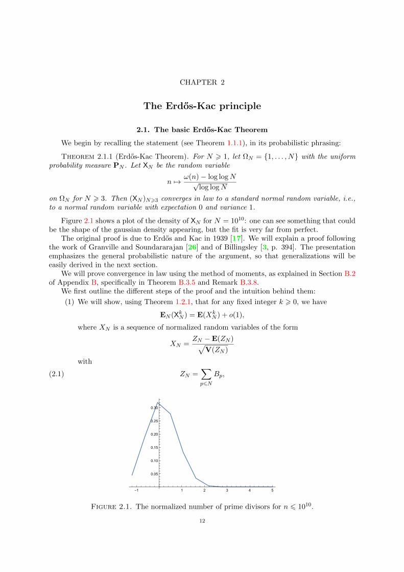
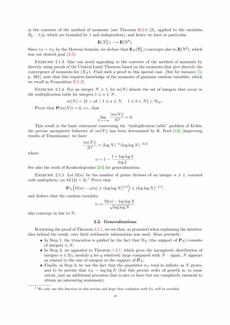
Figure 2.1 shows a plot of the density of XN for N = 1010: one can see something that couldbe the shape of the gaussian density appearing, but the fit is very far from perfect.
The original proof is due to Erdos and Kac in 1939 [17]. We will explain a proof followingthe work of Granville and Soundararajan [26] and of Billingsley [3, p. 394]. The presentationemphasizes the general probabilistic nature of the argument, so that generalizations will beeasily derived in the next section.
We will prove convergence in law using the method of moments, as explained in Section B.2of Appendix B, specifically in Theorem B.3.5 and Remark B.3.8.
We first outline the different steps of the proof and the intuition behind them:
(1) We will show, using Theorem 1.2.1, that for any fixed integer k > 0, we have
EN (XkN ) = E(XkN ) + o(1),
where XN is a sequence of normalized random variables of the form
XN =ZN −E(ZN )√
V(ZN )
with
(2.1) ZN =∑p6N
Bp,
-1 1 2 3 4 5
0.05
0.10
0.15
0.20
0.25
0.30
Figure 2.1. The normalized number of prime divisors for n 6 1010.
12
for some independent Bernoulli random variables (Bp)p indexed by primes and definedon some auxiliary probability space. The intuition behind this fact is quite simple: bydefinition, we have
(2.2) ω(n) =∑p|n
1 =∑p
Bp(n)
where Bp : Z −→ 0, 1 is the characteristic function of the multiples of p. In otherwords, Bp is obtained by composing the reduction map πp : Z −→ Z/pZ with thecharacteristic function of the residue class 0 ⊂ Z/pZ. For n ∈ ΩN , it is clear thatBp(n) = 0 unless p 6 N , and on the other hand, Proposition 1.2.5 (applied to thedifferent primes p 6 N) suggests that Bp, viewed as random variables on ΩN , are“almost” independent, while for N large, each Bp is “close” to a Bernoulli randomvariable Bp with
P(Bp = 1) =1
p, P(Bp = 0) = 1− 1
p.
(2) The Central Limit Theorem applies to the sequence (XN ), and shows that it convergesin law to a standard normal random variable N. This is not quite the most standardform of the Central Limit Theorem, since the summands Bp defining XN are notidentically distributed, but it is nevertheless a very simple and well-known case (seeTheorem B.5.1).
(3) It follows that
limN→+∞
EN (XkN ) = E(Nk),
and hence, by the method of moments (Theorem B.3.5), we conclude thatXN convergesin law to N. (Interestingly, we do not need to know the value of the moments E(Nk)for this argument to apply.)
This sketch shows that the Erdos-Kac Theorem is really a result of very general nature.Note that only Step 1 has real arithmetic content. As we will see, that arithmetic content isconcentrated on two results: Theorem 1.2.1, which makes the link with probability theory, andthe basic Mertens estimate from prime number theory∑
p6N
1
p= log logN +O(1)
for N > 3 (see Proposition C.1.1 in Appendix C). Indeed, this is where the normalization of thearithmetic function ω(n) comes from, and one could essentially dispense with this ingredient byreplacing the factors log logN in Theorem 2.1.1 by∑
p6N
1
p.
In order to prove such a statement, one only needs to know that this quantity tends to ∞ asN → +∞, which follows from the most basic statements concerning the distribution of primes,due to Chebychev.
We now implement those steps. As will be seen, some tweaks will be required. (Thereader is invited to check that omitting those tweaks leads, at the very least, to a much morecomplicated-looking problem!).
Step 1. (Truncation) This is a classical technique that applies here, and is used to shortenand simplify the sum in (2.1), in order to control the error terms in Step 2. We consider therandom variables Bp on ΩN as above, i.e., Bp(n) = 1 if p divides n and Bp(n) = 0 otherwise.Let
σN =∑p6N
1
p.
13
We only need recall at this point that σN → +∞ as N → +∞. We then define
(2.3) Q = N1/(log logN)1/3
and
ω(n) =∑p|np6Q
1 =∑p6Q
Bp(n), ω0(n) =∑p6Q
(Bp(n)− 1
p
),
viewed as random variables on ΩN . The point of this truncation is the following: first, forn ∈ ΩN , we have
ω(n) 6 ω(n) 6 ω(n) + (log logN)1/3,
simply because if α > 0 and if p1, . . . , pm are primes > Nα dividing n 6 N , then we get
Nmα 6 p1 · · · pm 6 N,
and hence m 6 α−1. Second, for any N > 1 and any n ∈ ΩN , we get by definition of σN theidentity
ω0(n) = ω(n)−∑p6Q
1
p
= ω(n)− σN +O((log logN)1/3)(2.4)
because the Mertens formula ∑p6x
1
p= log log x+O(1),
(see Proposition C.1.1) and the definition of σN show that∑p6Q
1
p=∑p6N
1
p+O(log log logN) = σN +O(log log logN).
Now define
XN (n) =ω0(n)√σN
as random variables on ΩN . We will prove that XN converges in law to N. The elementaryLemma B.3.3 of Appendix B (applied using (2.4)) then shows that the random variables
n 7→ ω(n)− σN√σN
converge in law to N. Finally, applying the same lemma one more time using the Mertensformula we obtain the Erdos-Kac Theorem.
It remains to prove the convergence of XN . We fix a non-negative integer k, and our targetis to prove the the moment limit
(2.5) EN (XkN )→ E(Nk)
as N → +∞. Once this is proved for all k, then the method of moments shows that (XN )converges in law to the standard normal random variable N.
Remark 2.1.2. We might also have chosen to perform a truncation at p 6 Nα for somefixed α ∈]0, 1[. However, in that case, we would need to adjust the value of α depending on k inorder to obtain (2.5), and then passing from the truncated variables to the original ones would
require some minor additional argument. In fact, the function (log logN)1/3 used to defined the
truncation could be replaced by any function going to infinity slower than (log logN)1/2.
14
Step 2. (Moment computation) We now begin the proof of (2.5). We use the definition of
ω0(n) and expand the k-th power in EN (XkN ) to derive
EN (XkN ) =1
σk/2N
∑p16Q
· · ·∑pk6Q
EN
((Bp1 −
1
p1
)· · ·(Bpk −
1
pk
)).
The crucial point is that the random variable
(2.6)(Bp1 −
1
p1
)· · ·(Bpk −
1
pk
)can be expressed as f(πq) for some modulus q > 1 and some function f : Z/qZ −→ C, so thatthe basic result of Theorem 1.2.1 may be applied to each summand.
To be precise, the value at n ∈ ΩN of the random variable (2.6) only depends on the residueclass x of n in Z/qZ, where q is the least common multiple of p1, . . . , pk. In fact, this value isequal to f(x) where
f(x) =(δp1(x)− 1
p1
)· · ·(δpk(x)− 1
pk
)with δpi denoting the characteristic function of the residues classes modulo q which are 0 modulopi. It is clear that |f(x)| 6 1, as product of terms which are all 6 1, and hence we have thebound
‖f‖1 6 q(this is extremely imprecise, as we will see later). From this we get∣∣∣EN
((Bp1 −
1
p1
)· · ·(Bpk −
1
pk
))−E(f)
∣∣∣ 6 2q
N6
2Qk
N
by Theorem 1.2.1.But by the definition of f , we also see that
E(f) = E((Bp1 −
1
p1
)· · ·(Bpk −
1
pk
))where the random variables (Bp) form a sequence of independent Bernoulli random variableswith P(Bp = 1) = 1/p (the (Bp) for p dividing q are realized concretely as the characteristicfunctions δp on Z/qZ with uniform probability measure).
Therefore we derive
EN (XkN ) =1
σk/2N
∑p16Q
· · ·∑pk6Q
E((Bp1 −
1
p1
)· · ·(Bpk −
1
pk
))+O(QkN−1)
)=( τNσN
)k/2E(Xk
N ) +O(Q2kN−1)
=( τNσN
)k/2E(Xk
N ) + o(1)
by our choice (2.3) of Q, where
τN =∑p6Q
1
p
(1− 1
p
)=∑p6Q
V(Bp)
and
XN =1√τN
∑p6Q
(Bp −
1
p
).
Step 3. (Conclusion) We now note that the version of the Central Limit Theorem recalledin Theorem B.5.1 applies to the random variables (Bp), and implies precisely that XN convergesin law to N. But moreover, the sequence (XN ) satisfies the uniform integrability assumption
15
in the converse of the method of moments (see Theorem B.3.6 (2), applied to the variablesBp − 1/p, which are bounded by 1 and independent), and hence we have in particular
E(XkN ) −→ E(Nk).
Since τN ∼ σN by the Mertens formula, we deduce that EN (XkN ) converges also to E(Nk), whichwas our desired goal (2.5).
Exercise 2.1.3. One can avoid appealing to the converse of the method of moments bydirectly using proofs of the Central Limit Theorem based on the moments that give directly theconvergence of moments for (XN ). Find such a proof in this special case. (See for instance [3,p. 391]; note that this requires knowledge of the moments of gaussian random variables, whichwe recall in Proposition B.5.2).
Exercise 2.1.4. For an integer N > 1, let m(N) denote the set of integers that occur inthe multiplication table for integers 1 6 n 6 N :
m(N) = k = ab | 1 6 a 6 N, 1 6 b 6 N ⊂ ΩN2 .
Prove that P(m(N)) = 0, i.e., that
limN→+∞
|m(N)|N2
= 0.
This result is the basic statement concerning the “multiplication table” problem of Erdos;the precise asymptotic behavior of |m(N)| has been determined by K. Ford [19] (improvingresults of Tenenbaum): we have
|m(N)|N2
(logN)−α(log logN)−3/2
where
α = 1− 1 + log log 2
log 2.
See also the work of Koukoulopoulos [34] for generalizations.
Exercise 2.1.5. Let Ω(n) be the number of prime divisors of an integer n > 1, countedwith multiplicity (so Ω(12) = 3).1 Prove that
PN
(Ω(n)− ω(n) > (log logN)1/4
)6 (log logN)−1/4,
and deduce that the random variables
n 7→ Ω(n)− log logN√log logN
also converge in law to N.
2.2. Generalizations
Reviewing the proof of Theorem 2.1.1, we see that, as promised when explaining the intuitiveidea behind the result, very little arithmetic information was used. More precisely:
• In Step 1, the truncation is guided by the fact that ΩN (the support of PN ) consistsof integers 6 N ;• In Step 2, we appealed to Theorem 1.2.1, which gives the asymptotic distribution of
integers n ∈ ΩN modulo q for q relatively large compared with N – again, N appearsas related to the size of integers in the support of PN ;• Finally, in Step 3, we use the fact that the quantities σN tend to infinity as N grows,
and to be precise that σN ∼ log logN (but this precise order of growth is, to someextent, just an additional precision that is nice to have but not completely essential toobtain an interesting statement).
1 We only use this function in this section and hope that confusion with ΩN will be avoided.
16
From this, it is not difficult to obtain a wide-ranging generalization of Theorem 2.1.1 toother sequences of integer-supported random variables. This is enough to deal for instance withthe measures associated to irreducible polynomials P ∈ Z[X] (as in Exercise 1.2.4), or to therandom walks on groups discussed in Section 1.3.2. However, we might want to consider thealso the distribution of ω(p − 1), for p prime, which is related instead to Section 1.3.1, andin this situation we lack the analogue of Theorem 1.2.1, as we observed (to be more precise,it would only follow from a close relative of the Generalized Riemann Hypothesis). But theproof of Step 2 shows that we are dealing there with how close the reduction of n modulo q, forn ∈ ΩN , to the limiting distribution µq, but rather to an average over q (namely, over q arisingas the lcm of primes p1, . . . , pk 6 Q). And, for primes, we do have some control over such anaverage by means of the Bombieri-Vinogradov estimates (1.6)!
Building on these observations, we can prove a very general abstract form of the Erdos-KacTheorem. (In a first reading, readers should probably just glance at the statement, and skip tothe examples, or to the next section or chapter, without looking at the proof, which is somethingof an exercice de style).
We begin by defining suitable sequences of random variables.
Definition 2.2.1. A balanced random integer is a sequence (XN )N>1 of random variableswith values in Z that satisfy the following properties:
(1) The expectation mN = E(|XN |) is finite, mN > 1, and mN tends to infinity as N → +∞;(2) There exist a real number θ > 0 and, for each integer q > 1, there exists a probability
measure µq on Z/qZ such that for any A > 0 and N > 1, we have∑q6mθN
max‖fq‖161
∣∣∣E(fq(πq(XN )))−Eµq(f)∣∣∣ 1
(log 2mN )A
where fq ranges over all functions fq : Z/qZ −→ C with ‖fq‖ 6 1, and the implied constantdepends on A.
Our main result essentially states that under suitable conditions, the number of prime factorsof a balanced random integer tends to a standard normal random variable. Here it will be usefulto use the convention ω(0) = 0.
Theorem 2.2.2 (General Erdos-Kac theorem). Let (XN ) be a balanced random integer.Assume furthermore that
(1) ...Then we have convergence in law
ω(XN )− σN√σN
−→ N
as N → +∞.
Proof. We first assume that XN takes values in Z− 0. For a given N , we define
τN =∑p6mN
µp(0)
and
Q = m1/τ
1/3N
N .
The assumption (??) ensures that Q→ +∞ as N → +∞. We then define the truncation
ω0,N =∑p6Q
(Bp −E(Bp))
where Bp is the Bernoulli random variable equal to 1 if and only if p | XN . We claim next thatif we define
σN =∑p6Q
µp(0),
17
then ω0,N/√σN converges in law to N.
To see this, we apply the method of moments. For a fixed integer k > 0, we have
E(( ω0,N√
σN
)k)=
1
σk/2N
∑p16Q
· · ·∑pk6Q
E(
(Bp1 −E(Bp1)) · · · (Bpk −E(Bpk))).
We rearrange the sum according to the value q of the lcm [p1, . . . , pk]. For each p = (p1, . . . , pk),there is a function fp : Z/qZ −→ R such that
(Bp1 −E(Bp1)) · · · (Bpk −E(Bpk)) = fp(πq(XN )).
Indeed, if ν(p) is the multiplicity of a divisor p of q in the tuple p, then we have
fp(x) =∏p|q
(δp(x)−E(Bp))ν(p).
Finally, we must deal with the case of random integers (XN ) that may take the value 0.
We do this by replacing the sequence (XN ) by (XN ) where XN is the restriction of XN to the
subset ΩN = XN 6= 0 of the original probability space, which is equiped with the conditionalprobability measure
PN (A) =P(A)
P(ΩN ).
We then haveω(XN )− σN√
σN−→ N
by the first case, and the result follows for (XN ) because
P(XN 6= 0) −→ 1.
2.3. Convergence without renormalization
One important point that is made clear by the proof of the Erdos-Kac Theorem is that,although one might think that a statement about the behavior of the number of primes factorsof integers tells us something about the distribution of primes (which are those integers nwith ω(n) = 1), the Erdos-Kac Theorem gives no information about these. This can be seenmechanically from the proof (where the truncation step means in particular that primes aredisregarded unless they are smaller than the truncation level Q), or intuitively from the factthat the statement itself implies that “most” integers of size about N have log logN primefactors. For instance, we have
PN
(|ω(n)− log logN | > a
√log logN
)−→ P(|N| > a) 6
√2
π
∫ +∞
ae−x
2/2dx 6 e−a2/4,
as N → +∞.The problem lies in the normalization used to obtain a definite theorem of convergence
in law: this “crushes” to some extent the more subtle aspect of the distribution of values ofω(n), especially with respect to extreme values. One can however still study this functionprobabilistically, but one must use less generic methods, to go beyond the “universal” behaviorgiven by the Central Limit Theorem. There are at least two possible approaches in this direction,and we now briefly survey some of the results.
Both methods have in common a switch in probabilistic focus: instead of looking for anormal approximation of a normalized version of ω(n), one looks for a Poisson approximationof the unnormalized function.
Recall (see also Section B.7 in the Appendix) that a Poisson distribution with real parameterλ > 0 satisfies
P(λ = k) = e−λλk
k!
18
2 4 6 8 10 12
0.05
0.10
0.15
0.20
0.25
0.30
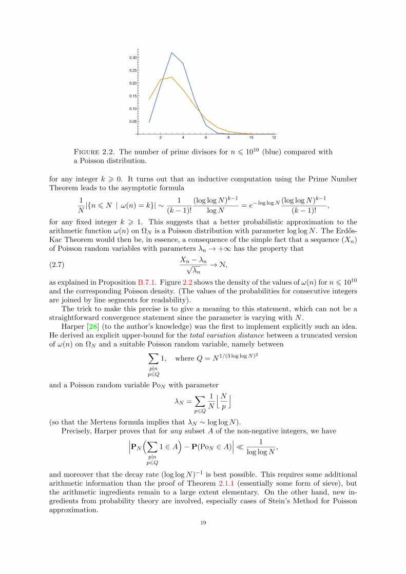
Figure 2.2. The number of prime divisors for n 6 1010 (blue) compared witha Poisson distribution.
for any integer k > 0. It turns out that an inductive computation using the Prime NumberTheorem leads to the asymptotic formula
1
N|n 6 N | ω(n) = k| ∼ 1
(k − 1)!
(log logN)k−1
logN= e− log logN (log logN)k−1
(k − 1)!,
for any fixed integer k > 1. This suggests that a better probabilistic approximation to thearithmetic function ω(n) on ΩN is a Poisson distribution with parameter log logN . The Erdos-Kac Theorem would then be, in essence, a consequence of the simple fact that a sequence (Xn)of Poisson random variables with parameters λn → +∞ has the property that
(2.7)Xn − λn√
λn→ N,
as explained in Proposition B.7.1. Figure 2.2 shows the density of the values of ω(n) for n 6 1010
and the corresponding Poisson density. (The values of the probabilities for consecutive integersare joined by line segments for readability).
The trick to make this precise is to give a meaning to this statement, which can not be astraightforward convergence statement since the parameter is varying with N .
Harper [28] (to the author’s knowledge) was the first to implement explicitly such an idea.He derived an explicit upper-bound for the total variation distance between a truncated versionof ω(n) on ΩN and a suitable Poisson random variable, namely between∑
p|np6Q
1, where Q = N1/(3 log logN)2
and a Poisson random variable PoN with parameter
λN =∑p6Q
1
N
⌊Np
⌋(so that the Mertens formula implies that λN ∼ log logN).
Precisely, Harper proves that for any subset A of the non-negative integers, we have∣∣∣PN
(∑p|np6Q
1 ∈ A)−P(PoN ∈ A)
∣∣∣ 1
log logN,
and moreover that the decay rate (log logN)−1 is best possible. This requires some additionalarithmetic information than the proof of Theorem 2.1.1 (essentially some form of sieve), butthe arithmetic ingredients remain to a large extent elementary. On the other hand, new in-gredients from probability theory are involved, especially cases of Stein’s Method for Poissonapproximation.
19
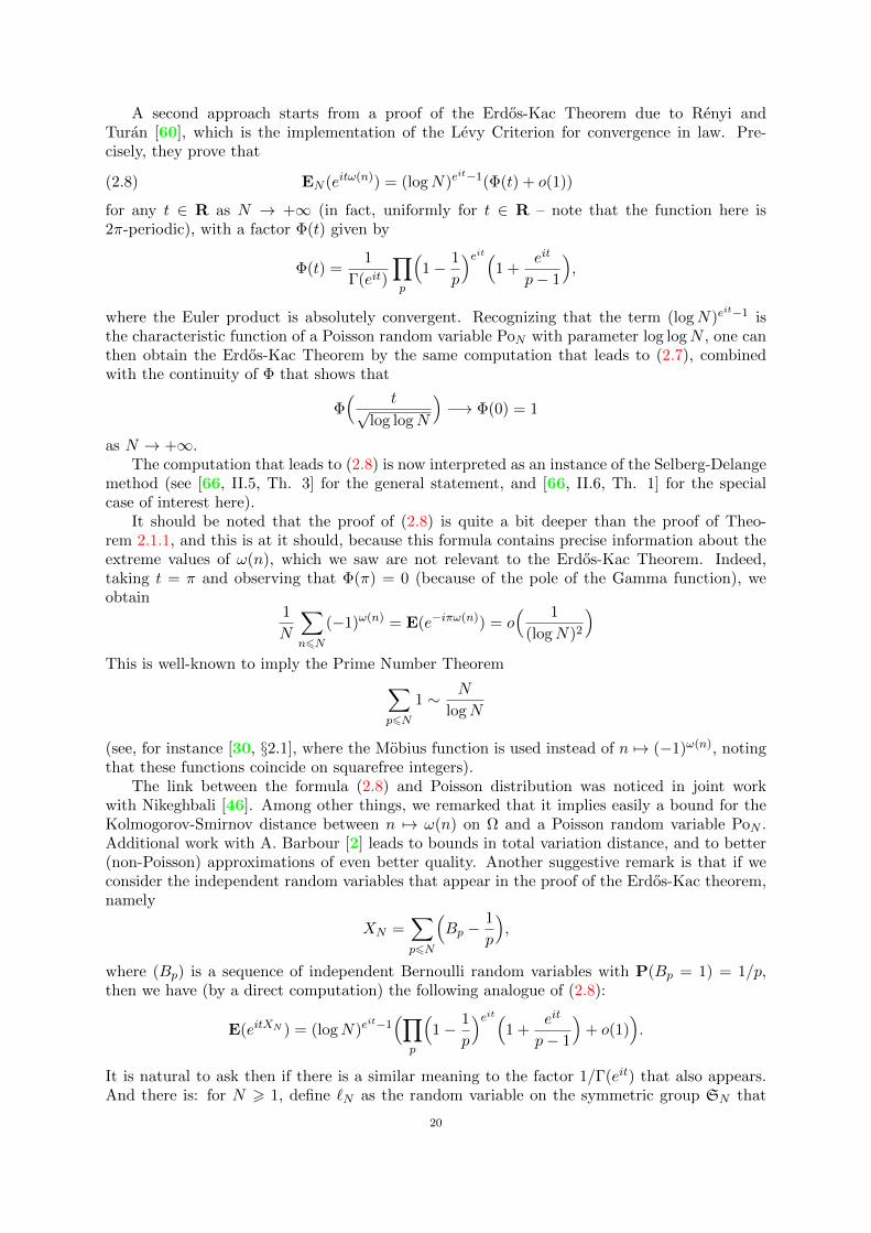
A second approach starts from a proof of the Erdos-Kac Theorem due to Renyi andTuran [60], which is the implementation of the Levy Criterion for convergence in law. Pre-cisely, they prove that
(2.8) EN (eitω(n)) = (logN)eit−1(Φ(t) + o(1))
for any t ∈ R as N → +∞ (in fact, uniformly for t ∈ R – note that the function here is2π-periodic), with a factor Φ(t) given by
Φ(t) =1
Γ(eit)
∏p
(1− 1
p
)eit(1 +
eit
p− 1
),
where the Euler product is absolutely convergent. Recognizing that the term (logN)eit−1 is
the characteristic function of a Poisson random variable PoN with parameter log logN , one canthen obtain the Erdos-Kac Theorem by the same computation that leads to (2.7), combinedwith the continuity of Φ that shows that
Φ( t√
log logN
)−→ Φ(0) = 1
as N → +∞.The computation that leads to (2.8) is now interpreted as an instance of the Selberg-Delange
method (see [66, II.5, Th. 3] for the general statement, and [66, II.6, Th. 1] for the specialcase of interest here).
It should be noted that the proof of (2.8) is quite a bit deeper than the proof of Theo-rem 2.1.1, and this is at it should, because this formula contains precise information about theextreme values of ω(n), which we saw are not relevant to the Erdos-Kac Theorem. Indeed,taking t = π and observing that Φ(π) = 0 (because of the pole of the Gamma function), weobtain
1
N
∑n6N
(−1)ω(n) = E(e−iπω(n)) = o( 1
(logN)2
)This is well-known to imply the Prime Number Theorem∑
p6N
1 ∼ N
logN
(see, for instance [30, §2.1], where the Mobius function is used instead of n 7→ (−1)ω(n), notingthat these functions coincide on squarefree integers).
The link between the formula (2.8) and Poisson distribution was noticed in joint workwith Nikeghbali [46]. Among other things, we remarked that it implies easily a bound for theKolmogorov-Smirnov distance between n 7→ ω(n) on Ω and a Poisson random variable PoN .Additional work with A. Barbour [2] leads to bounds in total variation distance, and to better(non-Poisson) approximations of even better quality. Another suggestive remark is that if weconsider the independent random variables that appear in the proof of the Erdos-Kac theorem,namely
XN =∑p6N
(Bp −
1
p
),
where (Bp) is a sequence of independent Bernoulli random variables with P(Bp = 1) = 1/p,then we have (by a direct computation) the following analogue of (2.8):
E(eitXN ) = (logN)eit−1
(∏p
(1− 1
p
)eit(1 +
eit
p− 1
)+ o(1)
).
It is natural to ask then if there is a similar meaning to the factor 1/Γ(eit) that also appears.And there is: for N > 1, define `N as the random variable on the symmetric group SN that
20
maps a permutation σ to the number of cycles in its canonical cyclic representation. Then,giving SN the uniform probability measure, we have
E(eit`N ) = N eit−1( 1
Γ(eit)+ o(1)
),
corresponding to a Poisson distribution with parameter logN this time. This is not an iso-lated property: see the survey paper of Granville [25] for many significant analogies between(multiplicative) properties of integers and random permutations.
Remark 2.3.1. Observe that (2.8) would be true if we had a decomposition
ω(n) = PoN (n) + YN (n)
as random variables on ΩN , where YN is independent of PoN and converges in law to a randomvariable with characteristic function Φ. However, this is not in fact the case, because Φ is nota characteristic function of a probability measure! (It is unbounded on R).
2.4. Further reading
21
CHAPTER 3
The distribution of values of the Riemann zeta function
3.1. Introduction
The Riemann zeta function is defined first for complex numbers s such that Re(s) > 1, bymeans of the series
ζ(s) =∑n>1
1
ns.
It plays an important role in prime number theory, arising because of the famous Euler productformula, which expresses ζ(s) as a product over primes, in this region: we have
(3.1) ζ(s) =∏p
(1− p−s)−1
if Re(s) > 1. By standard properties of series of holomorphic functions (note that s 7→ ns =es logn is entire for any n > 1), the Riemann zeta function is holomorphic for Re(s) > 1. It is ofcrucial importance however that it admits an analytic continuation to C−1, with furthermorea simple pole at s = 1 with residue 1.
This analytic continuation can be performed simultaneously with the proof of the functionalequation: the function defined by
Λ(s) = π−s/2Γ(s/2)ζ(s)
satisfies
Λ(1− s) = Λ(s).
Since ζ(s) is quite well-behaved for Re(s) > 1, and since the Gamma function is a very well-known function, this relation shows that one can understand the behavior of ζ(s) for s outsideof the critical strip
S = s ∈ C | 0 6 Re(s) 6 1.The Riemann Hypothesis is a crucial statement about ζ(s) when s is in the critical strip: itstates that if s ∈ S satisfies ζ(s) = 0, then the real part of s must be 1/2. Because holomorphicfunctions (with relatively slow growth, a property true for ζ, although this requires some argu-ment to prove) are essentially characterized by their zeros (just like polynomials are!), the proofof this conjecture would enormously expand our understanding of the properties of the Riemannzeta function. Although it remains open, this should motivate our interest in the distributionof values of the zeta function.
We first focus our attention to a vertical line Re(s) = τ , wehre τ is a fixed real numbersuch that τ > 1/2 (the case τ 6 1 will be the most interesting, but some statements do notrequire this assumption). We consider real numbers T > 2 and define the probability spaceΩT = [−T, T ] with the uniform probability measure dt/(2T ). We then view
t 7→ ζ(τ + it)
as a random variable Zτ,T on ΩT = [−T, T ]. These are arithmetically defined random variables.Do they have some specific, interesting, asymptotic behavior?
The answer to this question turns out to depend on τ , as the following first result reveals:
Theorem 3.1.1 (Bohr-Jessen). Let τ > 1/2 be a fixed real number. Define Zτ,T as therandom variable t 7→ ζ(τ + it) on ΩT . There exists a probability measure µτ on C such that
22
Zτ,T converges in law to µτ as T → +∞. Moreover, the support of µτ is compact if τ > 1, andis equal to C if 1/2 < τ 6 1.
We will describe precisely the measure µτ in Section 3.2: it is a highly non-generic probabilitydistribution, whose definition (and hence properties) retains a significant amount of arithmetic,in contrast with the Erdos-Kac Theorem, where the limit is a very generic distribution.
The analogue of Theorem 3.1.1 fails for τ = 1/2. This shows that the Riemann zeta functionis significantly more complicated on the critical line. However, there is a limit theorem afternormalization, due to Selberg, for the logarithm of the Riemann zeta function. To state it, wespecify carefully the meaning of log ζ(1
2 + it). We define a random variable LT on ΩT by puttingL(t) = 0 if ζ(1/2 + it) = 0, and otherwise
LT (t) = log ζ(12 + it),
where the logarithm of zeta is the unique branch that is holomorphic on a narrow strip
s = σ + iy ∈ C | σ > 12 − δ, |y − t| 6 δ
for some δ > 0, and satisfies log ζ(σ + it)→ 0 as σ → +∞.
Theorem 3.1.2 (Selberg). With notation as above, the random variables
LT√12 log log T
on ΩT converge in law as T → +∞ to a standard complex gaussian random variable.
There is another generalization of Theorem 3.1.1, due to Voronin [69] and Bagchi [1], thatwe will discuss, and that extends it in a very surprising direction. Instead of fixing τ ∈]1/2, 1[and looking at the distribution of the single values ζ(τ + it) as t varies, we consider for such τsome radius r such that the disc
D = s ∈ C | |s− τ | 6 ris contained in the interior of the critical strip, and we look for t ∈ R at the functions
ζD,t :
D −→ Cs 7→ ζ(s+ it)
which are “vertical translates” of the Riemann zeta function restricted to D. For each T > 0,we view t 7→ ζD,t as a random variable (say ZD,T ) on ([−T, T ], dt/(2T )) with values in thespace H(D) of functions which are holomorphic in the interior of D and continuous on itsboundary. Bagchi’s remarkable result is a convergence in law in this space: there exists aprobability measure ν on H(D) such that the random variables ZD,T converge in law to ν asT → +∞. Computing the support of ν (which is a non-trivial task) leads to a proof of Voronin’suniversality theorem: for any function f ∈ H(D) which does not vanish on D, and for any ε > 0,there exist t ∈ R such that
‖ζ(·+ it)− f‖∞ < ε,
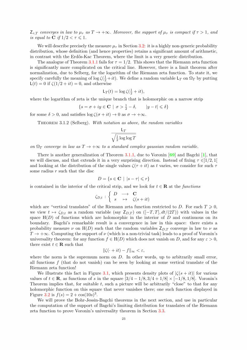
where the norm is the supremum norm on D. In other words, up to arbitrarily small error,all functions f (that do not vanish) can be seen by looking at some vertical translate of theRiemann zeta function!
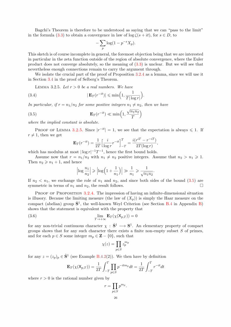
We illustrate this fact in Figure 3.1, which presents density plots of |ζ(s + it)| for variousvalues of t ∈ R, as functions of s in the square [3/4 − 1/8, 3/4 + 1/8] × [−1/8, 1/8]. Voronin’sTheorem implies that, for suitable t, such a picture will be arbitrarily “close” to that for anyholomorphic function on this square that never vanishes there; one such function displayed inFigure 3.2 is f(s) = 2 + cos(10s)3.
We will prove the Bohr-Jessin-Bagchi theorems in the next section, and use in particularthe computation of the support of Bagchi’s limiting distribution for translates of the Riemannzeta function to prove Voronin’s universality theorem in Section 3.3.
23
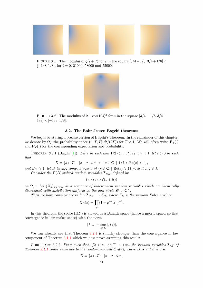
Figure 3.1. The modulus of ζ(s+ it) for s in the square [3/4−1/8, 3/4+1/8]×[−1/8, 1/8], for t = 0, 21000, 58000 and 75000.
Figure 3.2. The modulus of 2 + cos(10s)3 for s in the square [3/4− 1/8, 3/4 +1/8]× [−1/8, 1/8].
3.2. The Bohr-Jessen-Bagchi theorems
We begin by stating a precise version of Bagchi’s Theorem. In the remainder of this chapter,we denote by ΩT the probability space ([−T, T ], dt/(2T )) for T > 1. We will often write ET (·)and PT (·) for the corresponding expectation and probability.
Theorem 3.2.1 (Bagchi [1]). Let τ be such that 1/2 < τ . If 1/2 < τ < 1, let r > 0 be suchthat
D = s ∈ C | |s− τ | 6 r ⊂ s ∈ C | 1/2 < Re(s) < 1,and if τ > 1, let D be any compact subset of s ∈ C | Re(s) > 1 such that τ ∈ D.
Consider the H(D)-valued random variables ZD,T defined by
t 7→ (s 7→ ζ(s+ it))
on ΩT . Let (Xp)p prime be a sequence of independent random variables which are identicallydistributed, with distribution uniform on the unit circle S1 ⊂ C×.
Then we have convergence in law ZD,t −→ ZD, where ZD is the random Euler product
ZD(s) =∏p
(1− p−sXp)−1.
In this theorem, the space H(D) is viewed as a Banach space (hence a metric space, so thatconvergence in law makes sense) with the norm
‖f‖∞ = supz∈D|f(z)|.
We can already see that Theorem 3.2.1 is (much) stronger than the convergence in lawcomponent of Theorem 3.1.1 which we now prove assuming this result:
Corollary 3.2.2. Fix τ such that 1/2 < τ . As T → +∞, the random variables Zτ,T ofTheorem 3.1.1 converge in law to the random variable ZD(τ), where D is either a disc
D = s ∈ C | |s− τ | 6 r24

contained in the interior of the critical strip, if τ < 1, or any compact subset of s ∈ C |Re(s) > 1 such that τ ∈ D.
Proof. Fix D as in the statement. Tautologically, we have
Zτ,T = ζD,T (τ)
or Zτ,T = eτ ζD,T , where
eτ
H(D) −→ Cf 7→ f(τ)
is the evaluation map. Since this map is continuous for the topology on H(D), it is tautological(see Proposition B.2.1 in Appendix B) that the convergence in law ZD,T −→ ZD of Bagchi’sTheorem implies the convergence in law of Zτ,T to the random variable eτ ZD, which is simplyZD(τ).
In order to prove the final part of Theorem 3.1.1, and to derive Voronin’s universalitytheorem, we need to understand the support of the limit ZD in Bagchi’s Theorem. We willprove in Section 3.3:
Theorem 3.2.3 (Bagchi, Voronin). Let τ be such that 1/2 < τ < 1, and r such that
D = s ∈ C | |s− τ | 6 r ⊂ s ∈ C | 1/2 < Re(s) < 1.The support of the distribution of the law of ZD contains
H(D)× = f ∈ H(D) | f(z) 6= 0 for all z ∈ Dand is equal to H(D)× ∪ 0.
In particular, for any function f ∈ H(D)×, and for any ε > 0, there exists t ∈ R such that
(3.2) sups∈D|ζ(s+ it)− f(s)| < ε.
It is then obvious that if 1/2 < τ < 1, the support of the Bohr-Jessen random variableZD(τ) is equal to C.
We now begin the proof of Theorem 3.2.1 by giving some intuition for the result and inparticular for the shape of the limiting distribution. Indeed, this very elementary argumentwill suffice to prove Bagchi’s Theorem in the case τ > 1. This turns out to be similar to theintuition behind the Erdos-Kac Theorem. We begin with the Euler product
ζ(s+ it) =∏p
(1− p−s−it)−1,
which is valid for Re(s) > 1. We compute the logarithm
(3.3) log ζ(s+ it) = −∑p
log(1− p−s−it),
and see that this is a sum of random variables where the randomness lies in the behavior of thesequence of random variables (Xp,T )p on ΩT given by Xp(t) = p−it, which take values in the unit
circle S1. We view (Xp,T )p, for each T > 1, as taking value in the infinite product S1 =∏p S1
of circles parameterized by primes, which is still a compact metric space. It is therefore naturalto study the behavior of these sequences as T → +∞, in order to guess how ZD,T will behave.This has a very simple answer:
Proposition 3.2.4. For T > 0, let
XT = (Xp,T )p
be the S1-valued random variable on ΩT . given by
t 7→ (p−it)p.
Then XT converges in law as T → +∞ to a random variable X = (Xp)p, where the Xp areindependent and uniformly distributed on S1.
25
Bagchi’s Theorem is therefore to be understood as saying that we can “pass to the limit”in the formula (3.3) to obtain a convergence in law of log ζ(s+ it), for s ∈ D, to
−∑p
log(1− p−sXp).
This sketch is of course incomplete in general, the foremost objection being that we are interestedin particular in the zeta function outside of the region of absolute convergence, where the Eulerproduct does not converge absolutely, so the meaning of (3.3) is unclear. But we will see thatnevertheless enough connections remain to carry the argument through.
We isolate the crucial part of the proof of Proposition 3.2.4 as a lemma, since we will use itin Section 3.4 in the proof of Selberg’s Theorem.
Lemma 3.2.5. Let r > 0 be a real numbers. We have
(3.4) |ET (r−it)| 6 min(
1,1
T | log r|
).
In particular, if r = n1/n2 for some positive integers n1 6= n2, then we have
(3.5) ET (r−it) min(
1,
√n1n2
T
)where the implied constant is absolute.
Proof of Lemma 3.2.5. Since |r−it| = 1, we see that the expectation is always 6 1. Ifr 6= 1, then we get
ET (r−it) =1
2T
[ i
log rr−it
]T−T
=i(riT − r−iT )
2T (log r),
which has modulus at most | log r|−1T−1, hence the first bound holds.Assume now that r = n1/n2 with n1 6= n2 positive integers. Assume that n2 > n1 > 1.
Then n2 > n1 + 1, and hence∣∣∣logn1
n2
∣∣∣ > ∣∣∣log(
1 +1
n1
)∣∣∣ 1
n1>
1√n1n2
.
If n2 < n1, we exchange the role of n1 and n2, and since both sides of the bound (3.5) aresymmetric in terms of n1 and n2, the result follows.
Proof of Proposition 3.2.4. The impression of having an infinite-dimensional situationis illusory. Because the limiting measure (the law of (Xp)) is simply the Haar measure on the
compact (abelian) group S1, the well-known Weyl Criterion (see Section B.4 in Appendix B)shows that the statement is equivalent with the property that
(3.6) limT→+∞
ET (χ(Xp,T )) = 0
for any non-trivial continuous character χ : S1 −→ S1. An elementary property of compactgroups shows that for any such character there exists a finite non-empty subset S of primes,and for each p ∈ S some integer mp ∈ Z− 0, such that
χ(z) =∏p∈S
zmpp
for any z = (zp)p ∈ S1 (see Example B.4.2(2)). We then have by definition
ET (χ(Xp,T )) =1
2T
∫ T
−T
∏p∈S
p−itmpdt =1
2T
∫ T
−Tr−itdt
where r > 0 is the rational number given by
r =∏p∈S
pmp .
26
Since we have r 6= 1 (because S is not empty and mp 6= 0), we obtain ET (χ(Xp,T )) → 0 asT → +∞ from (3.4).
As a corollary, Bagchi’s Theorem follows formally for τ > 1 and D contained in the setof complex numbers with real part > 1. This is once more a very simple fact which is oftennot specifically discussed, but which gives an indication and a motivation for the more difficultstudy in the critical strip.
Special case of Theorem 3.2.1 for τ > 1. Assume that τ > 1 and that D is a compactsubset containing τ contained in s ∈ C | Re(s) > 1. We view XT = (Xp,T ) as random variables
with values in the topological space S1, as before. This is also (as a countable product of metricspaces) a metric space. We claim that the map
ϕ
S1 −→ H(D)
(xp) 7→(s 7→ −
∑p
log(1− xpp−s))
is continuous. If this is so, then the composition principle (see Proposition B.2.1) and Proposi-tion 3.2.4 imply that ϕ(XT ) converges in law to the H(D)-valued random variable ϕ(X), whereX = (Xp) with the Xp uniform and independent on S1. But this is exactly the statement ofBagchi’s Theorem for D.
Now we check the claim. Fix ε > 0. Let T > 0 be some parameter to be chosen later interms of ε. For any x = (xp) and y = (yp) in S1, we have
‖ϕ(x)− ϕ(y)‖∞ 6∑p6T
‖ log(1− xpp−s)− log(1− ypp−s)‖∞+
∑p>T
‖ log(1− xpp−s)‖∞ +∑p>T
‖ log(1− ypp−s)‖∞.
Because D is compact in the half-plane Re(s) > 1, the minimum of the real part of s ∈ Dis some real numbers σ0 > 1. Since |xp| = |yp| = 1 for all primes, and
| log(1− z)| 6 2|z|for |z| 6 1/2, it follows that∑
p>T
‖ log(1− xpp−s)‖∞ +∑p>T
‖ log(1− ypp−s)‖∞ 6 4∑p>T
p−σ0 T 1−σ0 .
We fix T so that T 1−σ0 < ε/2. Now the map
(xp)p6T 7→∑p6T
‖ log(1− xpp−s)− log(1− ypp−s)‖∞
is obviously continuous, and therefore uniformly continuous since the definition set is compact.This function has value 0 when xp = yp for p 6 T , so there exists δ > 0 such that∑
p6T
| log(1− xpp−s)− log(1− ypp−s)| <ε
2
if |xp − yp| 6 δ for p 6 T . Therefore, provided that
maxp6T|xp − yp| 6 δ,
we have‖ϕ(x)− ϕ(y)‖∞ 6 ε.
This proves the (uniform) continuity of ϕ.
We now begin the proof of Bagchi’s Theorem in the critical strip. The argument followsclosely his original proof [1], which is quite different from the Bohr-Jessen approach (as we willbriefly discuss at the end). Here are the main steps of the proof:
27
• We prove convergence almost surely of the random Euler product, and of its formalDirichlet series expansion; this also shows that they define random holomorphic func-tions;• We prove that both the Riemann zeta function and the limiting Dirichlet series are,
in suitable mean sense, limits of smoothed partial sums of their respective Dirichletseries;• We then use an elementary argument to conclude using Proposition 3.2.4.
We fix from now on a sequence (Xp)p of independent random variables all uniformly dis-
tributed on S1. We often view the sequence (Xp) as an S1-valued random variable. Furthermore,for any positive integer n > 1, we define
(3.7) Xn =∏p|n
Xvp(n)p
where vp(n) is the p-adic valuation of n. Thus (Xn) is a sequence of S1-valued random variables.
Exercise 3.2.6. Prove that the sequence (Xn)n>1 is neither independent nor symmetric.
We first show that the limiting random functions are indeed well-defined as H(D)-valuedrandom variables.
Proposition 3.2.7. Let τ ∈]1/2, 1[ and let Uτ = s ∈ C | <(s) > τ.(1) The random Euler product defined by
Z(s) =∏p
(1−Xpp−s)−1
converges almost surely for any s ∈ Uτ ; for any compact subset K ⊂ Uτ , the random function
ZK :
K −→ C
s 7→ Z(s)
is an H(K)-valued random variable.(2) The random Dirichlet series defined by
Z =∑n>1
Xnn−s
converges almost surely for any s ∈ Uτ ; for any compact subset K ⊂ Uτ , the random functionZK : s 7→ Z(s) on K is an H(K)-valued random variable, and moreover, we have ZK = ZKalmost surely.
Proof. (1) For N > 1 and s ∈ K we have∑p6N
log(1−Xpp−s)−1 =
∑p6N
Xp
ps+∑k>2
∑p6N
Xpk
pks.
Since Re(s) > 1/2 for s ∈ K, the series ∑k>2
∑p
Xpk
pks
converges absolutely for s ∈ Uτ . By Lemma A.2.1, its sum is therefore a random holomorphicfunction in H(K)-valued random variable for any compact subset K of Uτ .
Fix now τ1 < τ such that τ1 > 12 . We can apply Kolmogorov’s Theorem B.8.1 to the
independent random variables (Xpp−τ1), since∑
p
V(p−τ1Xp) =∑p
1
p2τ1< +∞.
28
Thus the series ∑p
Xp
pτ1
converges almost surely. By Lemma A.2.1 again, it follows that
P (s) =∑p
Xp
ps
converges almost surely for all s ∈ Uτ , and is holomorphic on Uτ . By restriction, its sum is anH(K)-valued random variable for any K compact in Uτ .
These facts show that the sequence of partial sums∑p6N
log(1−Xpp−s)−1
converges almost surely as N → +∞ to a random holomorphic function on K. Taking theexponential, we obtain the almost sure convergence of the random Euler product to a randomholomorphic function ZK on K.
(2) The argument is similar, except that the sequence (Xn)n>1 is not independent. However,it is orthonormal: if n 6= m, we have
E(XnXm) = 0, E(|Xn|2) = 1
(indeed Xn and Xm may be viewed as characters of S1, and they are distinct if n 6= m, so thatthis is the orthogonality property of characters of compact groups). We can then apply theMenshov-Rademacher Theorem B.8.4 to (Xn) and an = n−τ1 : since∑
n>1
|an|2(log n)2 =∑n>1
(log n)2
n2τ1< +∞,
the series∑Xnn
−τ1 converges almost surely, and Lemma A.2.1 shows that Z converges almost
surely on Uτ , and defines a holomorphic function there. Restricting to K leads to ZK asH(K)-valued random variable.
Finally, to prove that ZK = ZK almost surely, we may replace K by the compact subset
K1 = s ∈ C | τ1 6 σ 6 A, |t| 6 B,with A > 2 and B chosen large enough to ensure that K ⊂ K1. The previous argument showsthat the random Euler product and Dirichlet series converge almost surely on K1. But K1
contains the open set
V = s ∈ C | 1 < Re(s) < 2, |t| < Bwhere the Euler product and Dirichlet series converge absolutely, so that Lemma C.2.4 provesthat the random holomorphic functions ZK1 and ZK1 are equal when restricted to V . Byanalytic continuation (and continuity), they are equal also on K1, hence a posteriori on K.
We will prove Bagchi’s Theorem using the random Dirichlet series, which is easier to handlethan the Euler product. However, we will still denote it Z(s), which is justified by the last partof the proposition.
For the proof of Bagchi’s Theorem, some additional properties of this random Dirichletseries are needed. Most importantly, we need to find a finite approximation that also applies tothe Riemann zeta function. This will be done using smooth partial sums.
First we need to check that Z(s) is of polynomial growth on average on vertical strips.
Lemma 3.2.8. Let Z(s) be the random Dirichlet series∑Xnn
−s defined and holomorphicalmost surely for Re(s) > 1/2. For any σ1 > 1/2, we have
E(|Z(s)|) 1 + |s|uniformly for all s such that Re(s) > σ1.
29
Proof. The series ∑n>1
Xn
nσ1
converges almost surely. Therefore the partial sums
Su =∑n6u
Xn
nσ1
are bounded almost surely.By summation by parts (see Appendix A), it follows that for any s with real part σ > σ1,
we have
Z(s) = (s− σ1)
∫ +∞
1
Suus−σ1+1
du,
where the integral converges almost surely. Hence
|Z(s)| 6 (1 + |s|)∫ +∞
1
|Su|uσ−σ1+1
du.
Fubini’s Theorem (for non-negative functions) and the Cauchy-Schwarz inequality then imply
E(|Z(s)|) 6 (1 + |s|)∫ +∞
1E(|Su|)
du
uσ−σ1+1
6 (1 + |s|)∫ +∞
1E(|Su|2)1/2 du
uσ−σ1+1
= (1 + |s|)∫ +∞
1
(∑n6u
1
n2σ1
)1/2 du
uσ−σ1+1 1 + |s|,
using the orthonormality of the variables Xn.
We can then deduce a good result on average approximation by partial sums.
Proposition 3.2.9. Let ϕ : [0,+∞[−→ [0, 1] be a smooth function with compact supportsuch that ϕ(0) = 1. Let ϕ denote its Mellin transform. For N > 1, define the H(D)-valuedrandom variable
ZD,N =∑n>1
Xnϕ( nN
)n−s.
There exists δ > 0 such that
E(‖ZD − ZD,N‖∞) N−δ
for N > 1.
We recall that the norm ‖ · ‖∞ refers to the sup norm on the compact set D.
Proof. The first step is to apply the smoothing process of Proposition A.2.3 in Appendix A.The random Dirichlet series
Z(s) =∑n>1
Xnn−s
converges almost surely for Re(s) > 1/2. For σ > 1/2 and any δ > 0 such that
−δ + σ > 1/2,
we have therefore almost surely the representation
(3.8) ZD(s)− ZD,N (s) = − 1
2iπ
∫(−δ)
Z(s+ w)ϕ(w)Nwdw
for s ∈ D. (Figure 3.3 may help understand the location of the regions involved in the proof).Note that here are below, it is important that the “almost surely” property holds for all
s; this is simply because we work with random variables taking values in H(D), and not withparticular evaluations of these random functions at a specific s ∈ D.
30
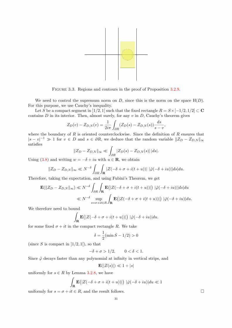
Figure 3.3. Regions and contours in the proof of Proposition 3.2.9.
We need to control the supremum norm on D, since this is the norm on the space H(D).For this purpose, we use Cauchy’s inequality.
Let S be a compact segment in ]1/2, 1[ such that the fixed rectangle R = S×[−1/2, 1/2] ⊂ Ccontains D in its interior. Then, almost surely, for any v in D, Cauchy’s theorem gives
ZD(v)− ZD,N (v) =1
2iπ
∫∂R
(ZD(s)− ZD,N (s))ds
s− v,
where the boundary of R is oriented counterclockwise. Since the definition of R ensures that|s − v|−1 1 for v ∈ D and s ∈ ∂R, we deduce that the random variable ‖ZD − ZD,N‖∞satisfies
‖ZD − ZD,N‖∞ ∫∂R|ZD(s)− ZD,N (s)| |ds|.
Using (3.8) and writing w = −δ + iu with u ∈ R, we obtain
‖ZD − ZD,N‖∞ N−δ∫∂R
∫R|Z(−δ + σ + i(t+ u))| |ϕ(−δ + iu)||ds|du.
Therefore, taking the expectation, and using Fubini’s Theorem, we get
E(‖ZD − ZD,N‖∞) N−δ∫∂R
∫R
E(|Z(−δ + σ + i(t+ u))|
)|ϕ(−δ + iu)||ds|du
N−δ sups=σ+it∈R
∫R
E(|Z(−δ + σ + i(t+ u))|
)|ϕ(−δ + iu)|du.
We therefore need to bound∫R
E(|Z(−δ + σ + i(t+ u))|
)|ϕ(−δ + iu)|du.
for some fixed σ + it in the compact rectangle R. We take
δ =1
2(minS − 1/2) > 0
(since S is compact in ]1/2, 1[), so that
−δ + σ > 1/2, 0 < δ < 1.
Since ϕ decays faster than any polynomial at infinity in vertical strips, and
E(|Z(s)|) 1 + |s|uniformly for s ∈ R by Lemma 3.2.8, we have∫
RE(|Z(−δ + σ + i(t+ u))|
)|ϕ(−δ + iu)|du 1
uniformly for s = σ + it ∈ R, and the result follows.
31
The last preliminary result is a similar approximation result for the translates of the Riemannzeta function by smooth partial sums of its Dirichlet series.
Proposition 3.2.10. Let ϕ : [0,+∞[−→ [0, 1] be a smooth function with compact supportsuch that ϕ(0) = 1. Let ϕ denote its Mellin transform. For N > 1, define
ζN (s) =∑n>1
ϕ( nN
)n−s,
and define ZN,T to be the H(D)-valued random variable t 7→ (s 7→ ζN (s+ it)).There exists δ > 0 such that
ET (‖ZD,T − ZN,T ‖∞) N−δ +NT−1
for N > 1 and T > 1.
Note that ζN is an entire function, since ϕ has compact support, so that the range of thesum is in fact finite. The meaning of the statement is that the smoothed partial sums ζN givevery uniform and strong approximations to the vertical translates of the Riemann zeta function.
Proof. We will write ZT for ZD,T for simplicity. We begin by applying the smoothingprocess of Proposition A.2.3 in Appendix A in the case an = 1. For σ > 1/2 and any δ > 0such that −δ + σ > 1/2, we have (as in the previous proof) the representation
(3.9) ζ(s)− ζN (s) = − 1
2iπ
∫(−δ)
ζ(s+ w)ϕ(w)Nwdw −N1−sϕ(1− s)
where the second term comes from the fact that the Riemann zeta function has a pole at s = 1with residue 1.
As before, let S be a compact segment in ]1/2, 1[ such that the fixed rectangle R = S ×[−1/2, 1/2] ⊂ C contains D in its interior. Then for any v with Re(v) > 1/2 and t ∈ R,Cauchy’s theorem gives
ζ(v + it)− ζN (v + it) =1
2iπ
∫∂R
(ζ(s+ it)− ζN (s+ it))ds
s− v,
where the boundary of R is oriented counterclockwise, and using |s − v|−1 1 for v ∈ D ands ∈ ∂R, we deduce that the random variable ‖ZT − ZN,T ‖∞, which takes the value
sups∈D|ζ(s+ it)− ζN (s+ it)|
at t ∈ ΩT , satisfies
‖ZT − ZN,T ‖∞ ∫∂R|ζ(s+ it)− ζN (s+ it)||ds|
for t ∈ ΩT . Taking the expectation with respect to t (i.e., integrating over t ∈ [−T, T ]) andapplying Fubini’s Theorem for non-negative functions leads to
ET
(‖ZT − ZN,T ‖∞
)∫∂R
ET
(|ζ(s+ it)− ζN (s+ it)|
)|ds|
sups∈∂R
ET
(|ζ(s+ it)− ζN (s+ it)|
).(3.10)
We take again δ = 12(minS − 1/2) > 0, so that 0 < δ < 1. For any fixed s = σ + it ∈ ∂R, we
have
−δ + σ >1
2+ δ >
1
2.
Applying (3.9) and using again Fubini’s Theorem, we obtain
ET
(|ζ(s+ it)− ζN (s+ it)|
) N−δ
∫R|ϕ(−δ + iu)|ET
(|ζ(σ − δ + i(t+ u))|
)du
+N1−σ ET (|ϕ(1− s− it)|).
32
The rapid decay of ϕ on vertical strips shows that the second term (arising from the pole)is NT−1. In the first term, since σ − δ > min(S)− δ > 1
2 + δ, we have
(3.11) ET
(|ζ(σ − δ + i(t+ u))|
)=
1
2T
∫ T
−T|ζ(σ − δ + i(t+ u))|dt 1 +
|u|T 1 + |u|
by Proposition C.3.1 in Appendix C. Hence
(3.12) ET
(|ζ(s+ it)− ζN (s+ it)|
) N−δ
∫R|ϕ(−δ + iu)|(1 + |u|)du+NT−1.
Now the fast decay of ϕ(s) on the vertical line Re(s) = −δ shows that the last integral isbounded, and we conclude from (3.10) that
ET
(‖ZT − ZN,T ‖∞
) N−δ +NT−1,
as claimed.
Finally we can prove Theorem 3.2.1:
Proof of Bagchi’s Theorem. By Proposition B.2.2, it is enough to prove that for anybounded and Lipschitz function f : H(D) −→ C, we have
ET (f(ZD,T )) −→ E(f(ZD))
as T → +∞. We may use the Dirichlet series expansion of ZD according to Proposition 3.2.7,(2).
Since D is fixed, we omit it from the notation for simplicity, denoting ZT = ZD,T andZ = ZD. Fix some integer N > 1 to be chosen later. We denote
ZT,N =∑n>1
n−s−itϕ( nN
)(viewed as random variable defined for t ∈ [−T, T ]) and
ZN =∑n>1
Xnn−sϕ
( nN
)the smoothed partial sums of the Dirichlet series as in Propositions 3.2.10 and 3.2.9.
We then write
|ET (f(ZT ))−E(f(Z))| 6 |ET (f(ZT )− f(ZT,N ))|+|ET (f(ZT,N ))−E(f(ZN ))|+ |E(f(ZN )− f(Z))|.
Since f is a Lipschitz function on H(D), there exists a constant C > 0 such that
|f(x)− f(y)| 6 C‖x− y‖∞for all x, y ∈ H(D). Hence we have
|ET (f(ZT ))−E(f(Z))| 6 C ET (‖ZT − ZT,N‖∞)+
|ET (f(ZT,N ))−E(f(ZN ))|+ C E(‖ZN − Z‖∞).
Fix ε > 0. Propositions 3.2.10 and 3.2.9 together show that there exists some N > 1 andsome constant C1 > 0 such that
ET (‖ZT − ZT,N‖∞) < ε+C1N
T
for all T > 1 and
E(‖ZN − Z‖∞) < ε.
33
We fix such a value of N . By Proposition 3.2.4 and composition, the random variables ZT,N(which are Dirichlet polynomials) converge in law to ZN as T → +∞. Since N/T → 0 also forT → +∞, we deduce that for all T large enough, we have
|ET (f(ZT ))−E(f(Z))| < 4ε.
This finishes the proof.
Exercise 3.2.11. Prove that if σ > 1/2 is fixed, then we have almost surely
limT→+∞
1
2T
∫ T
−T|Z(σ + it)|2dt = ζ(2σ).
[Hint. Use the Birkhoff-Khintchine pointwise ergodic theorem for flows, see e.g. [14, §8.6.1].]
3.3. The support of Bagchi’s measure
Our goal in this section is to explain the proof of Theorem 3.2.3, which is due to Bagchi [1,Ch. 5]. Since it involves results of complex analysis that are quite far from the main interestof these notes, we will only treat in detail the part of the proof that involves arithmetic, givingreferences for the results that are used.
The support is easiest to compute using the random Euler interpretation of the randomDirichet series, essentially because it is essentially a sum of independent random variables. Tobe precise, define
P (s) =∑p
Xp
ps, P (s) =
∑p
∑k>1
Xkp
pks
(see the proof of Proposition 3.2.7). The series converge almost surely for Re(s) > 1/2. We claim
that the support of the distribution of P , when viewed as an H(D)-valued random variable, isequal to H(D). Let us first assume this.
Since Z = exp(P ), we deduce by composition (see Lemma B.1.1) that the support of Z isthe closure of the set of functions of the form eg, where g ∈ H(D). But this last set is preciselyH(D)×, and Lemma A.3.5 in Appendix A shows that its closure in H(D) is H(D)× ∪ 0.
Finally, to prove the approximation property (3.2), which is the original version of Voronin’suniversality theorem, we simply apply Lemma B.2.4 to the family of random variables ZT , whichgives the much stronger statement that for any ε > 0, we have
lim infT→+∞
λ(t ∈ [−T, T ] | sups∈D|ζ(s+ it)− f(s)| < ε) > 0,
where λ denotes Lebesgue measure.From Proposition B.8.7 in Appendix B, the following proposition will imply that the support
of the random Dirichlet series P is H(D). The statement is slightly more general to help withthe last step afterwards.
Proposition 3.3.1. Let τ be such that 1/2 < τ < 1. Let r > 0 be such that
D = s ∈ C | |s− τ | 6 r ⊂ s ∈ C | 1/2 < Re(s) < 1.Let N be an arbitrary positive real number. The set of all series∑
p>N
xpps, (xp) ∈ S1,
which converge in H(D) is dense in H(D).
We will deduce the proposition from the density criterion of Theorem A.3.1 in Appendix A,applied to the space H(D) and the sequence (fp) with fp(s) = p−s for p prime. Since ‖fp‖∞ =p−σ1 , where σ1 = τ − r > 1/2, the condition∑
p
‖fp‖2∞ < +∞
34
holds. Furthermore, Proposition 3.2.7 certainly shows that there exist some (xp) ∈ S1 suchthat the series
∑p xpfp converges in H(D). Hence the conclusion of Theorem A.3.1 is what we
seek, and we only need to check the following lemma to establish the last hypothesis requiredto apply it:
Lemma 3.3.2. Let µ ∈ C(D)′ be a continuous linear functional. Let
g(z) = µ(s 7→ esz)
be its Laplace transform. If
(3.13)∑p
|g(log p)| < +∞,
then we have g = 0.
Indeed, the point is that µ(fp) = µ(s 7→ p−s) = g(log p), so that the assumption (3.13)concerning g is precisely (A.1).
This is a statement that has some arithmetic content, as we will see, and indeed the proofinvolves the Prime Number Theorem.
Proof. Let
% = lim supr→+∞
log |g(r)|r
,
which is finite by Lemma A.3.2 (1). By Lemma A.3.2 (3), it suffices to prove that % 6 1/2 toconclude that g = 0. To do this, we will use Theorem A.3.3, that provides access to the valueof % by “sampling” g along certain sequences of real numbers tending to infinity.
The idea is that (3.13) implies that |g(log p)| cannot be often of size at least 1/p = e− log p,since the series
∑p−1 diverges. Since the log p increase slowly, this makes it possible to find
real numbers rk → +∞ growing linearly and such that |g(rk)| 6 e−rk , and from this andTheorem A.3.3 we will get a contradiction.
To be precise, we first note that for y ∈ R, we have
|g(iy)| 6 ‖µ‖‖s 7→ eiys‖∞ 6 ‖µ‖er|y|
(since the maximum of the absolute value of the imaginary part of s ∈ D is r), and therefore
lim supy∈R|y|→+∞
log |g(iy)||y|
6 r.
We put α = r 6 1/4. Then the first condition of Theorem A.3.3 holds for the function g. Wealso take β = 1 so that αβ < π.
For any k > 0, let Ik be the set of primes p such that ek 6 p < ek+1. By the MertensFormula (C.1), or the Prime Number Theorem, we have∑
p∈Ik
1
p∼ 1
k
as k → +∞. Let further A be the set of those k > 0 for which the inequality
|g(log p)| > 1
p
holds for all primes p ∈ Ik, and let B be its complement among the non-negative integers. Wethen note that ∑
k∈A
1
k∑k∈A
∑p∈Ik
1
p∑k∈A
∑p∈Ik
|g(log p)| < +∞.
35
This shows that B is infinite. For k ∈ B, let pk be a prime in Ik such that |g(log pk)| < p−1k .
Let rk = log pk. We then have
lim supk→+∞
log |g(rk)|rk
6 −1.
Since pk ∈ Ik, we haverk = log pk ∼ k.
Furthermore, if we order B in increasing order, the fact that∑k/∈B
1
k< +∞
implies that the k-th element nk of B satisfies nk ∼ k.Now we consider the sequence formed from the r2k, arranged in increasing order. We have
r2k/k → 2 from the above. Moreover, by construction, we have
r2k+2 − r2k > 1,
hence |r2k − r2l| |k − l|. Since |g(r2k)| 6 e−r2k for all k ∈ B, we can apply Theorem A.3.3 tothis increasing sequence and we get
% = lim supk→+∞
log |g(r2k)|r2k
6 −1 < 1/2,
as desired.
There remains a last lemma to prove, that allows us to go from the support of the seriesP (s) of independent random variables to that of the full series P (s).
Lemma 3.3.3. The support of P (s) is H(D).
Proof. We can writeP = −
∑p
log(1−Xpp−s)
where the random variables (log(1−Xpp−s))p are independent, and the series converges almost
surely in H(D). Therefore it is enough by Proposition B.8.7 to prove that the set of convergentseries
−∑p
log(1− xpp−s), (xp) ∈ S1,
is dense in H(D).
Fix f ∈ H(D) and ε > 0 be fixed. For N > 1 and any (xp) ∈ S1, let
hN (s) =∑p>N
∑k>2
xkpkpks
.
This series converges absolutely for any s such that Re(s) > 1/2 and (xp) ∈ S1, and we have
‖hN‖∞ 6∑p>N
∑k>2
1
kpk/2→ 0
as N → +∞, uniformly with respect to (xp) ∈ S1. Fix N such that ‖hN‖∞ < ε2 for any
(xp) ∈ S1.Now let xp = 1 for p 6 N and define f0 ∈ H(D) by
f0(s) = f(s) +∑p6N
log(1− xpp−s).
For any choice of (xp)p>N such that the series∑p
xpps
36
defines an element of H(D), we can then write
f(s) +∑p
log(1− xpp−s) = gN (s) + f0(s) + hN (s),
for s ∈ D, where
gN (s) =∑p>N
xpps.
By Proposition 3.3.1, there exists (xp)p>N such that the series gN converges in H(D) and‖gN + f0‖∞ < ε
2 . We then have ∥∥∥f +∑p
log(1− xpp−s)∣∣∣ < ε.
Exercise 3.3.4. This exercises uses Voronin’s Theorem to deduce that the Riemann zetafunction is not the solution to any algebraic differential equation.
(1) For (a0, . . . , am) ∈ Cm+1 such that a0 6= 0, prove that there exists (b0, . . . , bm) ∈ Cm+1
such that we have
exp( m∑k=0
bksk)
=m∑k=0
akk!sk +O(sm+1)
for s ∈ C.Now fix a real number σ with 1
2 < σ < 1 and let g be a holomorphic function on C whichdoes not vanish.
(2) For any ε > 0, prove that there exists a real number t and r > 0 such that
sup|s|6r|ζ(s+ σ + it)− g(s)| < ε
rk
k!.
(3) Let n > 1 be an integer. Prove that there exists t ∈ R such that for all integers k with0 6 k 6 n− 1, we have
|ζ(k)(σ + it)− g(k)(0)| < ε.
(4) Let n > 1 be an integer. Prove that the image in Cn of the mapR −→ Cn
t 7→ (ζ(σ + it), . . . , ζ(n−1)(σ + it))
is dense in Cn.(5) Using (4), prove that if n > 1 and N > 1 are integers, and F0, . . . , FN are continuous
functions Cn → C, not all identically zero, then the function
N∑k=0
skFk(ζ(s), ζ ′(s), . . . , ζ(n−1)(s))
is not identically zero. In particular, the Riemann zeta function satisfies no algebraic differentialequation.
3.4. Selberg’s theorem
We present in this section a recent proof of “half” of Theorem 3.1.2 due to Radziwi l l andSoundararajan [56].
First, we (re)define the arithmetic random variables LT on ΩT by LT (t) = 0 if ζ(12 + it) = 0,
and otherwise LT (t) = log |ζ(12 + it)|. (Note the modulus, which means in particular that we
need not worry about the definition of the branch of the logarithm that we use).
37
Theorem 3.4.1 (Selberg). The random variables
LT√12 log log T
converge in law as T → +∞ to a standard real gaussian random variable.
The difference with Theorem 3.1.2 is that we only consider the modulus of ζ(1/2 + it), orin other words we consider only the real part of the random variables of Theorem 3.1.2.
In comparison with Bagchi’s Theorem, the strategy of the proof has the common feature ofthe use of suitable approximations to ζ, and it will ultimately derive the probabilistic behaviorfrom the independence and distribution of the vector t 7→ (p−it)p (as in Proposition 3.2.4).However, one has to be much more careful than in the previous section. The approximationused by Radziwi l l and Soundararajan involves three steps:
• Step 1: An approximation of LT by the random variable LT given by t 7→ log |ζ(σ0 +it)|for σ0 sufficiently close to 1/2 (where σ0 depends on T );
• Step 2: For the random variable ZT given by t 7→ ζ(σ0 + it), so that log |ZT | = LT , anapproximation of the inverse 1/ZT by a short Dirichlet polynomial DT of the type
DT (s) =∑n>1
aT (n)µ(n)n−s
where aT (n) is zero for n large enough (again, depending on T ); here µ(n) denotes theMobius function (see Definition C.2.3), which satisfies∑
n>1
µ(n)n−s =1
ζ(s)
if Re(s) > 1 (see Corollary C.2.5). At this point, we get an approximation of LT by− log |DT |;• Step 3: An approximation of |DT | by what is essentially a short Euler product, namely
by exp(−Re(PT )), where
(3.14) PT (t) =∑pk6X
1
k
1
pk(σ0+it)
for suitable X (again depending on T ). In this definition, and in all formulas involvingsuch sums below, the condition pk 6 X is implicitly restricted to integers k > 1. Atthis point, LT is approximated by Re(PT ).
Finally, the last probabilistic step is to prove that the random variables
Re(PT )√12 log log T
converge in law to a standard normal random variable as T → +∞.
None of these steps (except maybe the last) is especially easy, in comparison with the resultsdiscussed up to now, and the specific approximations that are used (namely, the choices of thecoefficients aT (n) as well as of the length parameter X) are quite subtle and by no meansobvious. Even the nature of the approximation will not be the same in the three steps!
In order to simplify the reading of the proof, we first specify the relevant parameters. We
assume from now on that T > ee2. We denote by
%T =√
12 log log T > 1,
38
the normalizing factor in the theorem. We then define
W = (log log log T )4 (log %T )4, σ0 =1
2+
W
log T=
1
2+O
((log %T )4
log T
)(3.15)
X = T 1/(log log log T )2 = T 1/√W .(3.16)
Note that we omit the dependency on T in most of these notation. We will also require a furtherparameter
(3.17) Y = T 1/(log log T )2 = T 4/%4 6 X.
We begin by stating the precise approximation statements. All parameters are now fixedas above for the remainder of this chapter. After stating the precise form of each steps of theproof, we will show how they combine to imply Theorem 3.4.1, and finally we will establishthese intermediate results.
Proposition 3.4.2 (Moving outside of the critical line). We have
ET
(|LT − LT |
)= o(%T )
as T → +∞.
We now define properly the Dirichlet polynomials that appear in the second step of theapproximation. It is here that the arithmetic subtlety lies, since the definition is quite delicate.We define first
(3.18) m1 = 100 log log T %T m2 = 100 log log log T log %T .
We denote by bT (n) the characteristic function of the set of squarefree integers n > 1 such thatall prime factors of n are 6 Y , and n has at most m1 prime factors. We denote by cT (n) thecharacteristic function of the set of squarefree integers n > 1 such that all prime factors p of nsatisfy Y < p 6 X, and n has at most m2 prime factors. We associate to these the Dirichletpolynomials
B(s) =∑n>1
µ(n)bT (n)n−s, C(s) =∑n>1
µ(n)cT (n)n−s
for s ∈ C. Finally, define D(s) = B(s)C(s). The coefficient of n−s in the expansion of D(s) isthe Dirichlet convolution∑
de=n
bT (d)cT (e)µ(d)µ(e) =∑de=n
(d,e)=1
bT (d)cT (e)µ(d)µ(e)
= µ(n)∑de=n
(d,e)=1
bT (d)cT (e) = µ(n)aT (n),
say, by Proposition A.2.4, where we used the fact that d and e are coprime if bT (d)cT (e) isnon-zero since the set of primes dividing an integer in the support of bT is disjoint from the setof primes dividing an integer in the support of cT . It follows then from this formula that aT (n)is the characteristic function of the set of squarefree integers n > 1 such that
(1) All prime factors of n are 6 X;(2) There are at most m1 prime factors p of n such that p 6 Y ;(3) There are at most m2 prime factors p of n such that Y < p 6 X.It is immediate, but very important, that aT (n) = 0 unless is quite small, namely
n 6 Y 100 log log TX100 log log log T = T c
where
c =100
log log T+
100
log log log T→ 0.
39
Finally, we define the arithmetic random variable
(3.19) DT = D(σ0 + it).
Remark 3.4.3. Although the definition of D(s) may seem complicated, we will see itsdifferent components coming together in the proofs of this proposition and the next.
If we consider the support of aT (n), we note that (by the Erdos-Kac Theorem, extendedto squarefree integers) the typical number of prime factors of an integer n 6 Y m1 is aboutlog log Y m1 ∼ log log T . Therefore the integers satisfying bT (n) = 1 are quite typical, and onlyextreme outliers (in terms of the number of prime factors) are excluded. On the other hand, theintegers satisfying cT (n) = 1 have much fewer prime factors than is typical, and are thereforequite rare (they are, in a weak sense, “almost prime”). This indicates that aT is a subtlearithmetic truncation of the characteristic function of integers n 6 T c, and hence that∑
n>1
aT (n)µ(n)n−s
is an arithmetic truncation of the Dirichlet series that formally gives the inverse of ζ(s). Thisshould be contrasted with the more traditional analytic truncations of ζ(s) that were used inLemma 3.2.8 and Proposition 3.2.9. For comparison, it is useful to note that Selberg himself used(for this purpose and for many other results concerning the Riemann zeta function) truncationsthat are roughly of the shape ∑
n6X
µ(n)
ns
(1− log n
logX
).
Proposition 3.4.4 (Dirichlet polynomial approximation). The difference ZTDT convergesto 1 in L2, i.e., we have
limT→+∞
ET
(|1− ZTDT |2
)= 0.
Proposition 3.4.5 (Euler product approximation). The random variables DT exp(−PT )converge to 1 in probability, i.e., for any ε > 0, we have
limT→+∞
PT
(|DT exp(PT )− 1| > ε
)= 0.
In particular, PT (DT = 0) tends to 0 as T → +∞.
Despite our probabilistic presentation, the three previous statement are really theorems ofnumber theory, and would usually be stated without probabilistic notation. For instance, thefirst one means that
1
T
∫ T
−T| log |ζ(1/2 + it)| − log |ζ(σ0 + it)||dt = o(log log T ).
The last result finally introduces the probabilistic behavior,
Proposition 3.4.6 (Normal Euler products). The random variables %−1T PT converge in law
as T → +∞ to a standard complex gaussian. In particular, the random variables
Re(PT )√12 log log T
converge in law to a standard normal random variable.
We will now explain how to combine these ingredients for the final step of the proof.
Proof of Theorem 3.4.1. Until Proposition 3.4.6 is used, this is essentially a variant ofthe fact that convergence in probability implies convergence in law, and that convergence in L1
or L2 implies convergence in probability.
40
For the details, fix some standard Gaussian random variable N. Let f be a bounded Lipschitzfunction R −→ R, and let C > 0 be a real number such that
|f(x)− f(y)| 6 C|x− y|, |f(x)| 6 C, for x, y ∈ R
We consider the difference ∣∣∣ET
(f(LT%T
))−E(f(N))
∣∣∣,and must show that this tends to 0 as T → +∞.
We estimate this quantity using the “chain” of approximations introduced above: we have
(3.20)∣∣∣ET
(f(LT%T
))−E(f(N))
∣∣∣ 6ET
(∣∣∣f(LT%T
)− f
( LT%T
)∣∣∣)+ ET
(∣∣∣f( LT%T
)− f
( log |DT |−1
%T
)∣∣∣)+
ET
(∣∣∣f( log |DT |−1
%T
)− f
(RePT%T
)∣∣∣)+∣∣∣ET
(f(RePT
%T
))−E(f(N))
∣∣∣,and we discuss each of the four terms on the right-hand side using the four previous propositions(here and below, we define |DT |−1 to be 0 if DT = 0).
The first term is handled straightforwardly using Proposition 3.4.2: we have
ET
(∣∣∣f(LT%T
)− f
( LT%T
)∣∣∣) 6 C
%TET (|LT − LT |) −→ 0
as T → +∞.For the second term, let AT ⊂ ΩT be the event
DT = 0 ∪ |LT − log |DT |−1| > 1/2,
and A′T its complement. Since log |ZT | = LT , we then have
ET
(∣∣∣f( LT%T
)− f
( log |DT |−1
%T
)∣∣∣) 6 2C PT (AT ) +C
2%T.
Proposition 3.4.4 implies that PT (AT )→ 0 (convergence to 1 of ZTDT in L2 implies convergenceto 1 in probability, hence convergence to 0 in probability for the logarithm of the modulus) andtherefore
ET
(∣∣∣f( LT%T
)− f
( log |DT |−1
%T
)∣∣∣)→ 0
as T → +∞.We now come to the third term on the right-hand side of (3.20). Distinguishing according
to the events
BT =∣∣log |DT exp(PT )|
∣∣ > 1/2
and its complement, we get as before
ET
(∣∣∣f( log |DT |−1
%T
)− f
(RePT%T
)∣∣∣) 6 2C PT (BT ) +C
2%T,
and this also tends to 0 as T → +∞ by Proposition 3.4.5.Finally, Proposition 3.4.6 implies that∣∣∣ET
(f(RePT
%T
))−E(f(N))
∣∣∣→ 0
as T → +∞, and hence we conclude the proof of the theorem, assuming the approximationstatements.
41
We now explain the proofs of these four propositions. We begin with the “easiest” part,which is also the where the transition to the probabilistic behavior enters. A key tool is thequantitative form of Proposition 3.2.4 contained in Lemma 3.2.5. More precisely, as in Sec-tion 3.2, let X = (Xp)p be a sequence of independent random variables uniformly distributedon S1. We define Xn for n > 1 by multiplicativity as in formula (3.7).
Lemma 3.4.7. Let (a(n))n>1 be any sequence of complex numbers with bounded support. Forany T > 2 and σ > 0, we have
ET
(∣∣∣∑n>1
a(n)
nσ+it
∣∣∣2) = E(∣∣∣∑n>1
Xn
nσ
∣∣∣2)+O( 1
T
∑m,n>1m 6=1
|a(m)a(n)|
(mn)σ−12
)
=∑n>1
|a(n)|2
n2σ+O
( 1
T
∑m,n>1m6=1
|a(m)a(n)|
(mn)σ−12
)where the implied constant is absolute.
Proof. We have
ET
(∣∣∣∑n>1
a(n)
nσ+it
∣∣∣2) =∑m
∑n
a(m)a(n)
(mn)σET
(( nm
)it).
We now apply Lemma 3.2.5 and separate the “diagonal” contribution where m = n from theremainder. This leads to the second formula in the lemma, and the first then simply reflectsthe orthonormality of the sequence (Xn)n>1.
When applying this lemma, we may call the first term the “diagonal” contribution, and thesecond the “off-diagonal” one.
Proof of Proposition 3.4.6. We have PT = QT + RT , where QT is the contribution ofthe primes, and RT the contribution of squares and higher powers of primes. We first claimthat RT is uniformly bounded in L2 for all T . Indeed, using Lemma 3.4.7, we get
ET (|RT |2) = ET
(∣∣∣∑k>2
∑p6X1/k
1
kp−kσ0p−kit
∣∣∣2)=∑pk6Xk>2
1
k2p−2kσ0 +O
( 1
T
∑k,l>2
∑pk,ql6Xp 6=q
1
kl(pq)−2σ0+
12
) 1 +
X2 logX
T 1
since X T ε for any ε > 0.From this, it follows that it is enough to show that QT /%T converges in law to a standard
complex gaussian random variable N. For this purpose, we use moments, i.e., we compute
ET
(QkTQ
`T
)for integers k, ` > 0, and we compare with the corresponding moment of the random variable
QT =∑p6X
p−σ0Xp.
After applying Lemma 3.2.5 again (as in the proof of Lemma 3.4.7), we find that
ET
(QkTQ
`T
)= E(QkTQ
`T ) +O
( 1
T
∑m 6=n
(mn)−σ0+1/2)
where the sum in the error term runs over integers m (resp. n) with at most k prime factors,counted with multiplicity, all of which are 6 X (resp. at most ` prime factors, counted with
42
multiplicity, all of which are 6 X). Hence this error term is
1
T
(∑p6X
1)k+`
Xk+`
T.
Next, we note that
V(QT ) =∑p6X
p−2σ0 V(X2p ) =
1
2
∑p6X
p−2σ0 .
We compute this sum by splitting in two ranges p 6 Y and Y < p 6 X. The second sum is
∑
Y <p6X
1
p= log
( logX
log Y
)+O(1) log log log T
by Proposition C.1.1 and (3.15). On the other hand, for p 6 Y = T 1/(log log T )2 , we have
p−2σ0 = p−1 exp(−2
W (log p)
(log T )
)= p−1
(1 +O
( W
(log log T )2
)),
which, in view of (3.15) implies that V(QT ) ∼ 12 log log T = %2
T as T → +∞.
It is again a case of the Central Limit Theorem that QT /√
V(QT ), hence also QT /%T ,converges in law to a standard complex gaussian random variable, with convergence of themoments (Theorem B.5.1 and Theorem B.3.6 (2), Remark B.3.7), so the conclusion followsfrom the method of moments, since Xk+`/T → 0 as T → +∞.
The other propositions will now be proved in order. Some of the arithmetic results that wewill used are only stated in Appendix C (with suitable references).
Proof of Proposition 3.4.2. We appeal to Hadamard’s factorization of the Riemannzeta function (Proposition C.3.2) in the form of its corollary, Proposition C.3.3. Let t ∈ ΩT besuch that there is no zero of zeta with ordinate t (this only excludes finitely many values of tfor a given T ). We have
log |ζ(σ0 + it)| − log |ζ(12 + it)| = Re
(∫ σ0
1/2
ζ ′
ζ(σ + it)dσ
)=
∫ σ0
1/2Re(ζ ′ζ
(σ + it))dσ.
For any σ with 12 6 σσ0, we have
−ζ′
ζ(σ + it) =
∑|t−Im(%)|<1
1
σ + it− %+O(log(2 + |t|)),
by Proposition C.3.3, where the sum is over zeros % of ζ(s) such that |σ + it− %| < 1.We fix t0 ∈ ΩT and integrate over t such that |t− t0| 6 1. This leads to∫ t0+1
t0−1
∣∣∣log |ζ(σ0 + it)| − log |ζ(12 + it)|
∣∣∣dt 6 ∑| Im(%)−t0|61
∫ t0+1
t0−1
∫ σ0
12
∣∣∣Re( 1
σ + it− %
)∣∣∣dtdσ.An elementary integral (!) gives∫ t0+1
t0−1
∣∣∣Re( 1
σ + it− %
)∣∣∣dt 6 ∫R
∣∣∣Re( 1
σ + it− %
)∣∣∣dt =
∫R
|σ − β|(σ − β)2 + (t− γ)2
dt = π
for all σ and %. Hence we get
1
T
∫|t−t0|61
∣∣∣log |ζ(12 + it− %)| − log |ζ(σ0 + it− %)|
∣∣∣dt (σ0 − 12)m(t0)
T,
where m(t0) is the number of zeros % such that |t0 − Im(%)| 6 1. This is log(2 + |t0|) byProposition C.3.3 again. Finally, by summing the bound
1
T
∫|t−t0|61
∣∣∣log |ζ(12 + it− %)| − log |ζ(σ0 + it− %)|
∣∣∣dt (σ0 − 12)
log(2 + |t0|)T
,
43
over a partition of ΩT in T intervals of length 2, we deduce that
ET (LT − LT |) (σ0 − 12) log T = W.
We have W = o(%T ) (by a rather wide margin!), and the proposition follows.
The last two propositions are more involved, and we present their proofs is separate sections
3.5. Dirichlet polynomial approximation
We will prove Proposition 3.4.4 in this section, i.e., we need to prove that
ET (|1− ZTDT |2),
where ZT (t) = ζ(σ0 + it), tends to 0 as T → +∞. This is arithmetically the most involved partof the proof.
First of all, we use the approximation formula
ζ(σ0 + it) =∑
16n6T
n−σ0−it +O(T 1−σ0
|t|+ 1+ T−1/2
)for t ∈ ΩT (see Proposition C.3.4). Multiplying by DT , we obtain
ET (ZTDT ) =∑m>1n6T
aT (m) ET ((mn)−σ0)+
O(T 1/2
∑m>1
aT (m) ET ((|t|+ 1)−1) + T−1/2∑m>1
aT (m)m−σ0).
We recall that |aT (n)| 6 1 for all n, and aT (n) = 0 unless n T ε, for any ε > 0. Hence,by (3.4), this becomes
ET (ZTDT ) = 1 +O( 1
T
∑n6Tm 6=n
aT (m)(mn)−σ0(logmn))
+O(T−1/2+ε)
= 1 +O(T−1/2+ε)
for any ε > 0 (in the diagonal terms, only m = n = 1 contributes, and in the off-diagonal termsmn 6= 1, we have ET ((mn)−it) T−1 log(mn)). It follows that it suffices to prove that
limT→+∞
ET (|ZTDT |2) = 1.
We expand the mean-square using the formula for DT , and obtain
ET (|ZTDT |2) =∑m,n
µ(m)µ(n)
(mn)σ0aT (m)aT (n) ET
((mn
)it|ZT |2
).
Now the asymptotic formula of Proposition C.3.5 translates to a formula for ET
((m/n)it|ZT |2
),
namely
ET
((mn
)it|ZT |2
)= ζ(2σ0)
((m,n)2
mn
)σ0+ ζ(2− 2σ0)
((m,n)2
mn
)1−σ0ET
(( |t|2π
)1−2σ0)+O(min(m,n)T−σ0+ε)
for any ε > 0, where the expectation is really the integral
1
2T
∫ T
−T
( |t|2π
)1−2σ0dt.
44
Using the properties of aT (n), the error term is easily handled, since it is at most
T−σ0+ε∑m,n
(mn)−σ0aT (m)aT (n) min(m,n) 6 T−σ0+ε(∑m
m1/2aT (m))2 T−σ0+2ε
for any ε > 0. Thus we only need to handle the main terms, which we write as
ζ(2σ0)M1 + ζ(2− 2σ0) ET
(( |t|2π
)1−2σ0)M2,
where
M1 =∑m,n
µ(m)µ(n)
(mn)2σ0aT (m)aT (n)(m,n)2σ0
and M2 is the other term. Using the multiplicative structure of aT , this factors in turn asM1 = M ′1M
′′1 , where
M ′1 =∑m,n
µ(m)µ(n)
[m,n]2σ0bT (m)bT (n),
M ′′1 =∑m,n
µ(m)µ(n)
[m,n]2σ0cT (m)cT (n).
We compare M ′1 to the similar sum M ′1 where bT (n) and bT (m) are replaced by characteristicfunctions of integers with all prime factors 6 Y , forgetting only the requirement that these have6 m1 prime factors. By Example C.2.6, we have
M ′1 =∏p6Y
(1− 1
p2σ0
).
The difference M ′1 − M ′1 can be bounded from above by
2e−m1∑m,n
|µ(m)µ(n)|[m,n]2σ0
eΩ(m)
where the sum runs over integers with all prime factors 6 Y (this step is a case of what is called“Rankin’s trick”: the condition Ω(m) > m1 is handled by bounding its characteristic function
by the non-negative function eΩ(m)−m1). Again from Example C.2.6, this is at most
2(log T )−100∏p6Y
(1 +
1 + 2e
p
) (log T )−90
(By Proposition C.1.4). Thus
M ′1 ∼∏p6Y
(1− p−2σ0)
as T → +∞. One deals similarly with the second term M ′′1 , which turns out to satisfy
M ′′1 ∼∏
Y <p6X
(1− p−2σ0),
and hence
M1 ∼ ζ(2σ0)∏p6X
(1− p−2σ0) =∏p>X
(1− p−2σ0).
Now, by the choice of the parameters, we obtain from the Prime Number Theorem (Theo-rem C.1.2) the upper-bound∑
p>X
p−2σ0 ∫ +∞
X
1
t2σ0dt
log t X1−2σ0
(2σ0 − 1) logX=X1−2σ0
2√W6
1
2√W.
45
Since this tends to 0 as T → +∞, it follows that∏p>X
(1− p−2σ0) = exp(∑p>X
( 1
p2σ0+O
( 1
p4σ0
))= exp
(−∑p>X
p−2σ0)
(1 + o(1))
converges to 1 as T → +∞.There only remains to check that the second part M2 of the main term tends to 0 as
T → +∞. We have
M2 =∑m,n
µ(m)µ(n)
mnaT (m)aT (n)(m,n)2−2σ0 =
∑m,n
µ(m)µ(n)
[m,n]2−2σ0aT (m)aT (n)(mn)1−2σ0 .
The procedure is very similar: we factor M2 = M ′2M′′2 , where M ′2 has coefficients bT instead of
aT , and M ′′2 has cT . Applying Example C.2.6 and Rankin’s Trick to both factors now leads to
M2 ∼∏p6X
(1 +
1
p2−2σ0
(− 1
p2σ0−1− 1
p2σ0−1+
1
p4σ0−2
))=∏p6X
(1− 2
p+
1
p2σ0
).
Now, however, we deduce from this that the contribution of M2 is
∼ ζ(2− 2σ0) ET
(( |t|2π
)1−2σ0) ∏p6X
(1− 2
p+
1
p2σ0
).
Since ζ(s) has a pole at s = 1 with residue 1, this last expression is
T 1−2σ0
2σ0 − 1
∏p6X
(1− 1
p
) T 1−2σ0
(2σ0 − 1) logX.
In terms of the parameter W , since 2σ0 − 1 = 2W/ log T and X = T 1/√W , the right-hand side
is simply exp(−2W )W−1/2, and hence tends to 0 as T → +∞. This concludes the proof.
3.6. Euler product approximation
This section is devoted to the proof of Proposition 3.4.5. We need to prove that DT exp(PT )converges to 1 in probability. This involves some extra decomposition of PT : we write
PT = QT + RT
where QT is the contribution to (3.14) of the prime powers pk 6 Y .In addition, for any integer m > 0, we denote by expm the Taylor polynomial of degree m
of the exponential function at 0, i.e.
expm(z) =m∑j=0
zj
j!.
We have an elementary lemma:
Lemma 3.6.1. Let z ∈ C and m > 0. If m > 100|z|, then
expm(z) = ez +O(exp(−m)) = ez(1 +O(exp(−99|z|))).
Proof. Indeed, since j! > (j/e)k for all j > 0 and |z| 6 m/100, the difference ez− expm(z)is at most ∑
j>m
(m/100)j
j!6∑j>m
( em
100j
)j exp(−m).
46
We define
ET = expm1(−QT ), FT = expm2
(−RT ),
where we recall that m1 and m2 are the parameters defined in (3.18). We have by definitionDT = BTCT , with
BT (t) =∑n>1
bT (n)µ(n)n−σ0−it, CT (t) =∑n>1
cT (n)µ(n)n−σ0−it,
where bT and cT are defined after the statement of Proposition 3.4.2, e.g., bT (n) is the charac-teristic function of squarefree integers n such that n has 6 m1 prime factors, all of which are6 Y .
The idea of the proof is that, usually, QT (resp. RT ) is not too large, and then the randomvariable ET is a good approximation to exp(−QT ). On the other hand, because of the shapeof ET (and the choice of the parameters), it will be possible to prove that ET is close to BT inL2-norm, and similarly for FT and CT . Combining these facts will lead to the conclusion.
We first observe that, as in the beginning of the proof of Proposition 3.4.6, by the usualappeal to Lemma 3.2.5, we have
ET (|QT |2) %T , ET (|RT |2) log %T .
Markov’s inequality implies that PT (|QT | > %T ) tends to 0 as T → +∞. Now by the lemmaabove, whenever |QT | 6 %T , we have
ET = exp(−QT )(
1 +O((log T )−99)).
Similarly, the probability PT (|RT | > log %T ) tends to 0, and whenever |RT | 6 log %T , we have
FT = exp(−RT )(
1 +O((log log T )−99)).
For the next step, we claim that
ET
(|ET − BT |2
) (log T )−60,(3.21)
ET
(|FT − CT |2
) (log log T )−60.(3.22)
We begin the proof of the first estimate with a lemma.
Lemma 3.6.2. For t ∈ ΩT , we have
ET (t) =∑n>1
α(n)n−σ0+it,
where the coefficients α(n) are zero unless n 6 Y m1 and has only prime factors 6 Y . More-over |α(n)| 6 1 for all n, and α(n) = µ(n)bT (n) if n has 6 m1 prime factors, counted withmultiplicity, and if there is no prime power pk dividing n such that pk > Y .
Proof. Since
ET = expm1(−QT ) =
m1∑j=0
(−1)j
j!
(∑pk6Y
1
kpk(σ0+it)
)j,
we obtain by expanding an expression as stated with coefficients
α(n) =∑
06j6m1
(−1)j
j!
∑pk11 ···p
kjj =n
pkii 6Y
1
k1 · · · kj.
We see from this expression that α(n) is 0 unless n 6 Y m1 and n has only prime factors 6 Y .Suppose now that n has 6 m1 prime factors, counted with multiplicity, and that no prime
47
power pk > Y divides n. Then we may extend the sum defining α(n) to all j > 0, and remove
the redundant conditions pkii 6 Y , so that
α(n) =∑j>0
(−1)j
j!
∑pk11 ···p
kjj =n
1
k1 · · · kj.
But we recognize that this is the coefficient of n−s in the expansion of
exp(−∑k>1
1
kp−ks
)= exp(− log ζ(s)) =
1
ζ(s)=∑n>1
µ(n)
ns,
(viewed as a formal Dirichlet series, or by restricting to Re(s) > 1). This means that, for suchintegers n, we have α(n) = µ(n) = µ(n)bT (n).
Finally, for any n > 1 now, we have
|α(n)| 6∑j>0
1
j!
∑pk11 ···p
kjj =n
1
k1 · · · kj= 1,
since the right-hand side is the coefficient of n−s in exp(log ζ(s)) = ζ(s).
Now define δ(n) = α(n)− µ(n)bT (n) for all n > 1. We have
ET
(|ET − BT |2
)= ET
(∣∣∣∑n>1
δ(n)
nσ0+it
∣∣∣2),which we estimate using Lemma 3.4.7. The contribution of the off-diagonal term is
1
T
∑m,n6Ym1
|δ(n)δ(m)|(mn)12−σ0 6
4
T
( ∑m6Ym1
1)2 T−1+ε
for any ε > 0, hence is negligible. The diagonal term is
M =∑n>1
|δ(n)|2
n2σ06∑n>1
|δ(n)|2
n.
By Lemma 3.6.2, we have δ(n) = 0 unless either n has > m1 prime factors, counted withmultiplicity, or is divisible by a power pk such that pk > Y (and necessarily p 6 Y since δ issupported on integers only divisible by such primes). The contribution of the integers satisfyingthe first property is at most ∑
Ω(n)>m1
p|n⇒p6Y
1
n.
We use Rankin’s trick once more to bound this from above: for any fixed real number η > 1,we have ∑
Ω(n)>m1
p|n⇒p6Y
1
n6 η−m1
∏p6Y
(1 +
η
p+ · · ·
) η−m1(log Y )η 6 (log T )−100 log η+η.
by Proposition C.1.4. Selecting η = e2/3 6 2, for instance, this shows that this contribution is (log T )−60.
The contribution of integers divisible by pk > Y is at most(∑p6Ypk>Y
1
pk
)( ∑p|n⇒p6Y
1
n
)6
1
Y
( ∑√Y <pk6Yk>2
1) ∏p6Y
1
1− p−1 Y −1/2(log Y ),
which is even smaller. This concludes the proof of (3.21).
48
The proof of the second estimate (3.22) is quite similar, with one extra consideration tohandle. Indeed, arguing as in Lemma 3.6.2, we obtain the expression
FT (t) =∑n>1
β(n)n−σ0+it,
for t ∈ ΩT , where the coefficients β(n) are zero unless n 6 Xm2 and has only prime factors6 X, satisfy |β(n)| 6 1 for all n, and finally satisfy β(n) = µ(n) if n has 6 m2 prime factors,counted with multiplicity, and if there is no prime power pk dividing n with Y < pk 6 X.
Using this, and defining now δ(n) = β(n)−µ(n)cT (n), we get from Lemma 3.4.7 the bound
ET
(|FT − CT |2
)
∑n>1δ(n) 6=0
1
n2σ06∑n>1δ(n)6=0
1
n.
But the integers that satisfy δ(n) 6= 0 must be of one of the following types:(1) Those with cT (n) = 1, which (by the preceeding discussion) must either have Ω(n) > m2
(and be divisible by primes 6 X only), or must be divisible by a prime power pk such thatpk > X (the possibility that pk 6 Y is here excluded, because cT (n) = 1 implies that n hasno prime factor < Y ). The contribution of these integers is handled as in the case of thebound (3.21) and is (log log T )−60.
(2) Those with cT (n) = 0 and β(n) 6= 0; since
β(n) =∑
06j6m2
(−1)j
j!
∑pk11 ···p
kjj =n
Y <pkii 6X
1
k1 · · · kj,
as in the beginning of the proof of Lemma 3.6.2, such an integer n has at least one factorization
n = pk11 · · · pkjj for some j 6 m2, where each prime power pkii is between Y and X. Since
cT (n) = 0, either Ω(n) > m2, or n has a prime factor p > X, or n has a prime factor p 6 Y .The first two possibilities are again handled exactly like in the proof of (3.21), but the third issomewhat different. We proceed as follows to estimate its contribution, say N . We have
N =∑
06j<m2
Nj ,
where
Nj =∑p6Y
∑n=pkp
k11 ···p
kjj
Y <pkii 6X
1
n
is the contribution of integers with a factorization of length j + 1 as a product of prime powersbetween Y and X. By multiplicativity, we get
Nj 6(∑p6Y
∑Y <pk6X
1
pk
) (∑p6X
∑Y <pk6X
1
pk
)j−1.
Consider the first factor. For a given prime p 6 Y , let l be the smallest integer such that pl > Y .The sum over k is then ∑
Y <pk6X
1
pk6
1
pl+
1
pl+1+ · · · 1
pl6
1
Y,
so that the first factor is π(Y )/Y (log Y )−1. On the other hand, for the second factor, wehave ∑
p6X
∑Y <pk6X
1
pk=∑p6Y
∑Y <pk6X
1
pk+
∑Y <p6X
∑Y <pk6X
1
pk π(Y )
Y+
∑Y <p6X
∑Y <pk6X
1
pk,
49
where we used the first result. For a given prime p with Y < p 6 X, the last sum over k is
1
p+
1
p2+ · · · 1
p,
and the sum over p is therefore∑Y <p6X
1
p= log
( logX
log Y
)+O(1) = log log log T +O(1),
using the values of X and Y and Proposition C.1.1. Hence the final estimate is
N 1
log Y(log log log T )m2 (log log T )(log log log T )m2(log T )−1 → 0
as T → +∞, from which we finally deduce that (3.22) holds.With the mean-square estimates (3.21) and (3.22) in hand, we can now finish the proof of
Proposition 3.4.6. Except on sets of measure tending to 0 as T → +∞, we have
BT = ET +O((log T )−25), ET = exp(−QT )(
1 +O((log T )−99))
1
log T6 exp(−QT ) 6 (log T )
(where the first property follows from (3.21)), and it hence
BT = exp(−QT )(
1 +O((log T )−20)),
again outside of a set of measure tending to 0. Similarly, using (3.22), we get
CT = exp(−RT )(
1 +O((log log T )−20))
outside of a set of measure tending to 0. Multipliying the two equalities shows that
DT = exp(−PT )(
1 +O((log log T )−20))
with probability tending to 1 as T → +∞. This concludes the proof.
Remark 3.6.3. It is instructive to see what happens if one varies the parameters, especiallyif one tries to use a single range pk 6 X instead of bringing the additional decomposition pk 6 Yor Y < pk 6 X. TODO
3.7. Further topics
If we look back at the proof of Bagchi’s Theorem, and at the proof of Voronin’s Theorem,we can see precisely which arithmetic ingredients appeared. They are the following:
• The crucial link between the arithmetic objects and the probabilistic model is providedby Proposition 3.2.4, which depends on the unique factorization of integers into primes;this is an illustration of the asymptotic independence of prime numbers, similarly toProposition 1.2.5;• The proof of Bagchi’s theorem then relies on the mean-value property (3.11) of the
Riemann zeta function; this estimate has arithmetic meaning (through the large sieveinequalities that enter into its proof, and also through its generalizations, as brieflydescribed below);• The Prime Number Theorem, which appears in the proof of Voronin’s Theorem, in
order to control the distribution of primes in (roughly) dyadic intervals.
Note that some arithmetic features remain in the Random Dirichlet Series that arises asthe limit in Bagchi’s Theorem, in contrast with the Erdos-Kac Theorem, where the limit is theuniversal gaussian distribution. This means, in particular, that going beyond Bagchi’s Theoremto applications (as in Voronin’s Theorem) still naturally involves arithmetic problems, many
50
of which are very interesting in their interaction with probability theory (see below for a fewreferences).
We thus see a clean separation of specific arithmetic arguments. In view of this, it is notvery surprising that Bagchi’s Theorem can be generalized to many other situations. The mostinteresting concerns perhaps the limiting behavior, in H(D), of families of L-functions of thetype
L(f, s) =∑n>1
λf (n)n−s
where f runs over some sequence of arithmetic objects with associated L-functions, ordered in asequence of probability spaces (which need not be continuous like ΩT ). We refer to [30, Ch. 5]for a survey and discussion of L-functions, and to [38] for a discussion of families of L-functions.There are some rather obvious special cases, such as the vertical translates L(χ, s+ it) of a fixedDirichlet L-function L(χ, s), since all properties of the Riemann zeta function extend to thiscase. Another interesting case is the finite set Ωq of non-trivial Dirichlet characters modulo aprime number q, with the uniform probability measure. Then one can look at the distributionof the restrictions to D of the Dirichlet L-functions L(s, χ) for χ ∈ Ωq, and indeed one cancheck that Bagchi’s Theorem extends to this situation.
A second exemple, which is treated in [41] is, still for a prime q > 2, the set Ωq of holomorphiccuspidal modular forms of weight 2 and level q, either with the uniform probability measure ofwith that provided by the Petersson formula ([38, 31, ex. 8]). An analogue of Bagchi’s Theoremholds, but the limiting random Dirichlet series is not the same as in Theorem 3.2.1: with thePetersson average, it is
(3.23)∏p
(1−Xpp−s + p−2s)−1,
where (Xp) is a sequence of independent random variables, which are all distributed accordingto the Sato-Tate measure (the same that appears in Example B.4.1 (3)). This different limitis simply due to the form that “local spectral equidistribution” (in the sense of [38]) takes forthis family (see [38, 38]). Indeed, the local spectral equidistribution property plays the role ofProposition 3.2.4. The analogue of (3.11) follows from a stronger mean-square formula, usingCauchy’s inequality: there exists a constant A > 0 such that, for any σ0 > 1/2 and all s ∈ Cwith Re(s) > σ0, we have
(3.24)∑f∈Ωq
ωf |L(f, s)|2 (1 + |s|)A
for q > 2, where ωf is the Petersson-averaging weight (see [45, Prop. 5], which proves an even
more difficult result where Re(s) can be as small as 12 + c(log q)−1).
However, extending Bagchi’s Theorem to many other families of L-functions (e.g., verticaltranslates of an L-function of higher rank) requires restrictions, in the current state of knowledge.The reason is that the analogue of the mean-value estimates (3.11) or (3.24) is usually onlyknown when Re(s) > σ0 > 1/2, for some σ0 such that σ0 < 1. Then the only domains D forwhich one can prove a version of Bagchi’s Theorem are those contained in Re(s) > σ0.
Generalizations of Selberg’s Central Limit Theorem are much harder to come by. Indeed,there are very few cases others than that of the Riemann zeta function where such a statement isknown (see the remarks in [56, §7] for references). For instance, consider the family of modularforms f as above. The natural question is now to consider the distribution (possibly withweights ωf ) of L(f, 1
2). First, it is a known fact (due to Waldspurger and Kohnen-Zagier) that
L(f, 12) > 0 in that case. This property reflects a different type of expected distribution of the
values L(f, 12), namely one expects that the correct normalization is
f 7→logL(f, 1
2) + 12 log log q
√log log q
,
51
in the sense that this defines a sequence of random variables on Ωq that should converge inlaw to a standard (real) gaussian random variable. Now observe that such a statement, if true,would immediately imply that the propertion of f ∈ Ωq with L(f, 1
2) = 0 tends to 0 as q → +∞,and this is not currently known (this would indeed be a major result in the analytic theory ofmodular forms).
Nevertheless, there has been significant progress in this direction, for various families, inrecent and ongoing work of Radziwi l l and Soundararajan. In [57], they prove subgaussian upperbounds for the distribution of L-values in certain families similar to Ωq (specifically, quadratictwists of a fixed modular form). In [58], they announce gaussian lower bounds, but for familiesconditioned to have L(f, 1
2) 6= 0 (which, for a number of cases, is known to be a subfamily withpositive density as the size tends to infinity).
One of the reasons that Central Limit Theorems are expected to hold is that they are knownto follow from the widely believed moment conjectures for families of L-functions, which predict(with considerable evidence, theoretic, numerical and heuristic) the asymptotic behavior of theLaplace or Fourier transform of the logarithm of the special values of the L-functions. In otherwords, for the Riemann Zeta function, these conjectures, due first to Keating and Snaith [33],predict the asymptotic behavior of
ET (es log |ζ( 12 +it)|) = ET (|ζ(1
2 + it)|s) =1
2T
∫ T
−T|ζ(1
2 + it)|sdt
for suitable s ∈ C. It is of considerable interest that, besides natural arithmetic factors (relatedto the independence of Proposition 3.2.4 or suitable analogues), these conjectures involve certainterms which originate in Random Matrix Theory. In addition to implying straightforwardly theCentral Limit Theorem, note that the moment conjectures also immediately yield the general-ization of (3.11) or (3.24), hence can be allowed to deduce general versions of Bagchi’s Theoremand universality. Moreover, these moment conjectures (in suitably uniform versions) are alsoable to settle other interesting conjectures concerning the distribution of values of ζ(1
2 + it). Forinstance, as shown by Kowalski and Nikeghbali [47], they are known to imply that the imageof t 7→ ζ(1
2 + it), for t ∈ R, is dense in C (a conjecture of Ramachandra).
[Further references: Titchmarsh [68], especially Chapter 11, discusses the older work ofBohr and Jessen, which has some interesting geometric aspects that are not apparent in moderntreatments. Bagchi’s Thesis [1] contains some generalizations as well as more information con-cerning the limit theorem and Voronin’s Theorem. The papers of Radziwi l l and Soundararajanare the most enlightening concerning the status of gaussian approximations of special valuesof L-functions. For families of L-functions and for the conjectures that would refine Selberg’sTheorem and its potential generalizations, based on Random Matrix Theory, see the work ofKeating-Snaith [33] and Katz-Sarnak [32] and of Kowalski and Nikeghbali [47]. For an intro-duction to many aspects of families of L-functions and their applications, see the introductionto the monograph [5] of Blomer, Fouvry, Kowalski, Michel, Milicevic and Sawin.]
52
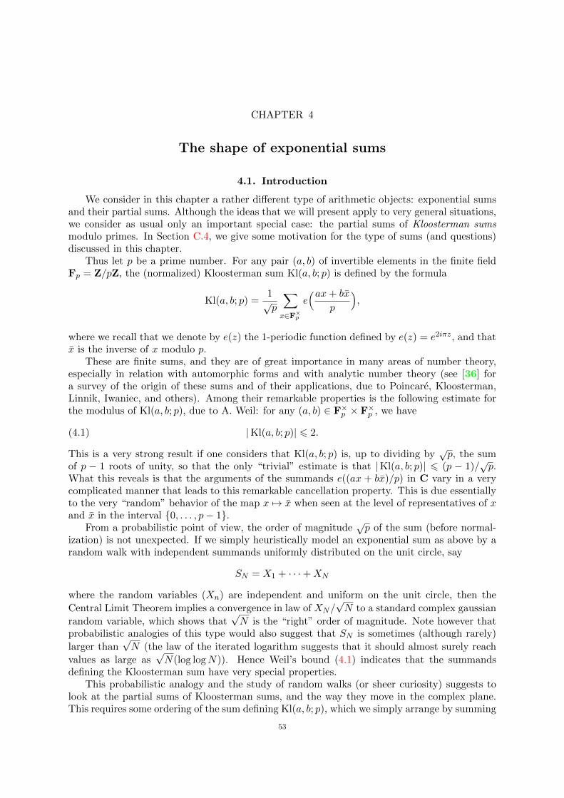
CHAPTER 4
The shape of exponential sums
4.1. Introduction
We consider in this chapter a rather different type of arithmetic objects: exponential sumsand their partial sums. Although the ideas that we will present apply to very general situations,we consider as usual only an important special case: the partial sums of Kloosterman sumsmodulo primes. In Section C.4, we give some motivation for the type of sums (and questions)discussed in this chapter.
Thus let p be a prime number. For any pair (a, b) of invertible elements in the finite fieldFp = Z/pZ, the (normalized) Kloosterman sum Kl(a, b; p) is defined by the formula
Kl(a, b; p) =1√p
∑x∈F×p
e(ax+ bx
p
),
where we recall that we denote by e(z) the 1-periodic function defined by e(z) = e2iπz, and thatx is the inverse of x modulo p.
These are finite sums, and they are of great importance in many areas of number theory,especially in relation with automorphic forms and with analytic number theory (see [36] fora survey of the origin of these sums and of their applications, due to Poincare, Kloosterman,Linnik, Iwaniec, and others). Among their remarkable properties is the following estimate forthe modulus of Kl(a, b; p), due to A. Weil: for any (a, b) ∈ F×p × F×p , we have
(4.1) |Kl(a, b; p)| 6 2.
This is a very strong result if one considers that Kl(a, b; p) is, up to dividing by√p, the sum
of p − 1 roots of unity, so that the only “trivial” estimate is that |Kl(a, b; p)| 6 (p − 1)/√p.
What this reveals is that the arguments of the summands e((ax + bx)/p) in C vary in a verycomplicated manner that leads to this remarkable cancellation property. This is due essentiallyto the very “random” behavior of the map x 7→ x when seen at the level of representatives of xand x in the interval 0, . . . , p− 1.
From a probabilistic point of view, the order of magnitude√p of the sum (before normal-
ization) is not unexpected. If we simply heuristically model an exponential sum as above by arandom walk with independent summands uniformly distributed on the unit circle, say
SN = X1 + · · ·+XN
where the random variables (Xn) are independent and uniform on the unit circle, then the
Central Limit Theorem implies a convergence in law of XN/√N to a standard complex gaussian
random variable, which shows that√N is the “right” order of magnitude. Note however that
probabilistic analogies of this type would also suggest that SN is sometimes (although rarely)
larger than√N (the law of the iterated logarithm suggests that it should almost surely reach
values as large as√N(log logN)). Hence Weil’s bound (4.1) indicates that the summands
defining the Kloosterman sum have very special properties.This probabilistic analogy and the study of random walks (or sheer curiosity) suggests to
look at the partial sums of Kloosterman sums, and the way they move in the complex plane.This requires some ordering of the sum defining Kl(a, b; p), which we simply arrange by summing
53
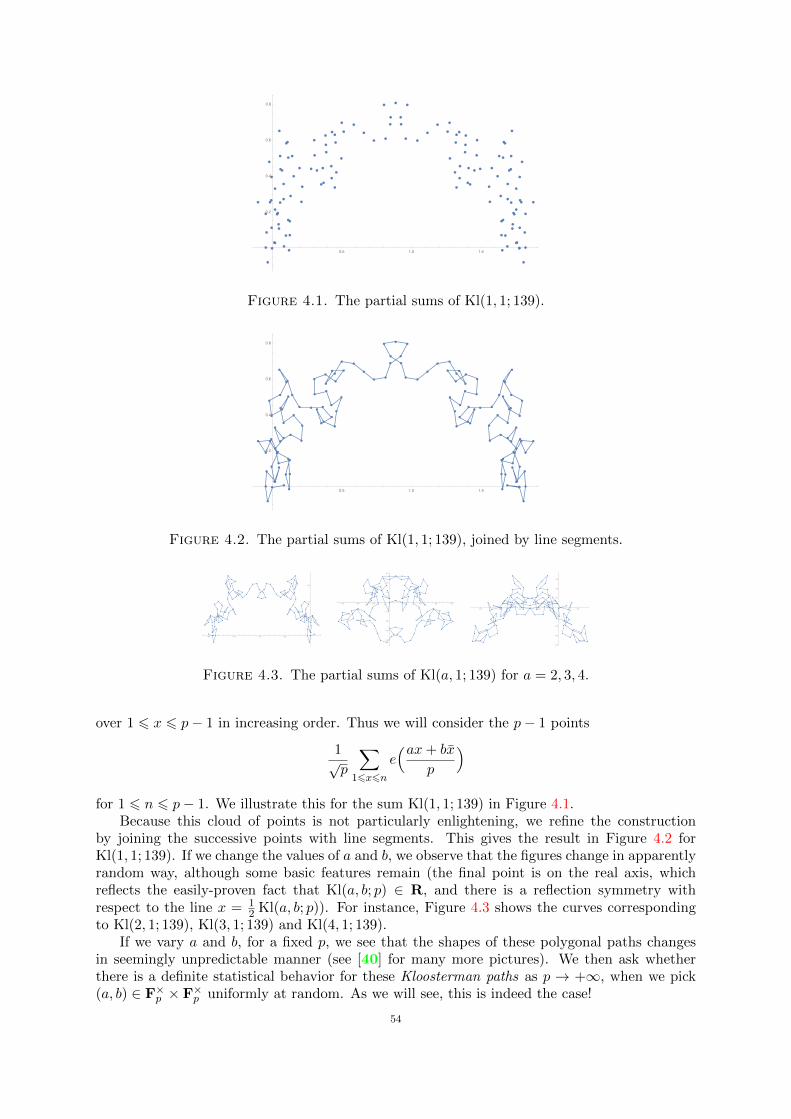
0.5 1.0 1.5
0.2
0.4
0.6
0.8
Figure 4.1. The partial sums of Kl(1, 1; 139).
0.5 1.0 1.5
0.2
0.4
0.6
0.8
Figure 4.2. The partial sums of Kl(1, 1; 139), joined by line segments.
-2.0 -1.5 -1.0 -0.5
0.2
0.4
0.6
-0.6 -0.4 -0.2 0.2 0.4 0.6 0.8
-0.4
-0.3
-0.2
-0.1
0.1
0.2
0.3
-0.8 -0.6 -0.4 -0.2 0.2
-0.4
-0.3
-0.2
-0.1
0.1
0.2
0.3
Figure 4.3. The partial sums of Kl(a, 1; 139) for a = 2, 3, 4.
over 1 6 x 6 p− 1 in increasing order. Thus we will consider the p− 1 points
1√p
∑16x6n
e(ax+ bx
p
)for 1 6 n 6 p− 1. We illustrate this for the sum Kl(1, 1; 139) in Figure 4.1.
Because this cloud of points is not particularly enlightening, we refine the constructionby joining the successive points with line segments. This gives the result in Figure 4.2 forKl(1, 1; 139). If we change the values of a and b, we observe that the figures change in apparentlyrandom way, although some basic features remain (the final point is on the real axis, whichreflects the easily-proven fact that Kl(a, b; p) ∈ R, and there is a reflection symmetry withrespect to the line x = 1
2 Kl(a, b; p)). For instance, Figure 4.3 shows the curves correspondingto Kl(2, 1; 139), Kl(3, 1; 139) and Kl(4, 1; 139).
If we vary a and b, for a fixed p, we see that the shapes of these polygonal paths changesin seemingly unpredictable manner (see [40] for many more pictures). We then ask whetherthere is a definite statistical behavior for these Kloosterman paths as p → +∞, when we pick(a, b) ∈ F×p × F×p uniformly at random. As we will see, this is indeed the case!
54
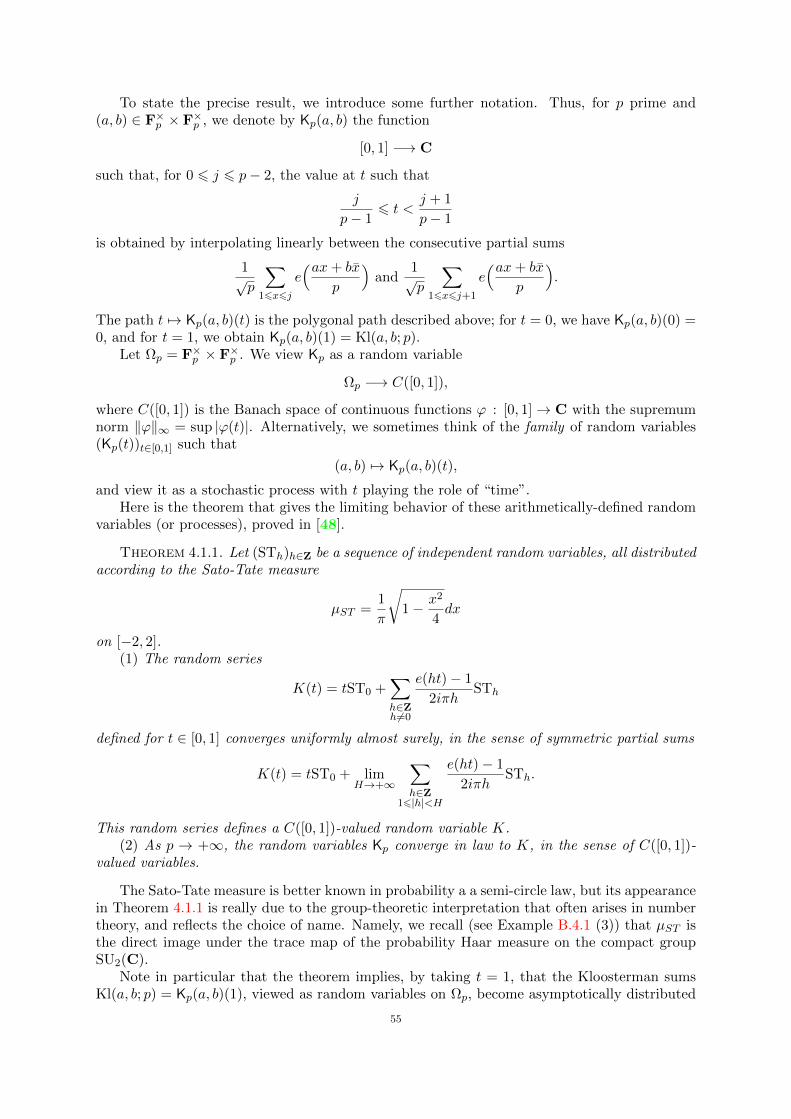
To state the precise result, we introduce some further notation. Thus, for p prime and(a, b) ∈ F×p × F×p , we denote by Kp(a, b) the function
[0, 1] −→ C
such that, for 0 6 j 6 p− 2, the value at t such that
j
p− 16 t <
j + 1
p− 1
is obtained by interpolating linearly between the consecutive partial sums
1√p
∑16x6j
e(ax+ bx
p
)and
1√p
∑16x6j+1
e(ax+ bx
p
).
The path t 7→ Kp(a, b)(t) is the polygonal path described above; for t = 0, we have Kp(a, b)(0) =0, and for t = 1, we obtain Kp(a, b)(1) = Kl(a, b; p).
Let Ωp = F×p × F×p . We view Kp as a random variable
Ωp −→ C([0, 1]),
where C([0, 1]) is the Banach space of continuous functions ϕ : [0, 1]→ C with the supremumnorm ‖ϕ‖∞ = sup |ϕ(t)|. Alternatively, we sometimes think of the family of random variables(Kp(t))t∈[0,1] such that
(a, b) 7→ Kp(a, b)(t),
and view it as a stochastic process with t playing the role of “time”.Here is the theorem that gives the limiting behavior of these arithmetically-defined random
variables (or processes), proved in [48].
Theorem 4.1.1. Let (STh)h∈Z be a sequence of independent random variables, all distributedaccording to the Sato-Tate measure
µST =1
π
√1− x2
4dx
on [−2, 2].(1) The random series
K(t) = tST0 +∑h∈Zh6=0
e(ht)− 1
2iπhSTh
defined for t ∈ [0, 1] converges uniformly almost surely, in the sense of symmetric partial sums
K(t) = tST0 + limH→+∞
∑h∈Z
16|h|<H
e(ht)− 1
2iπhSTh.
This random series defines a C([0, 1])-valued random variable K.(2) As p → +∞, the random variables Kp converge in law to K, in the sense of C([0, 1])-
valued variables.
The Sato-Tate measure is better known in probability a a semi-circle law, but its appearancein Theorem 4.1.1 is really due to the group-theoretic interpretation that often arises in numbertheory, and reflects the choice of name. Namely, we recall (see Example B.4.1 (3)) that µST isthe direct image under the trace map of the probability Haar measure on the compact groupSU2(C).
Note in particular that the theorem implies, by taking t = 1, that the Kloosterman sumsKl(a, b; p) = Kp(a, b)(1), viewed as random variables on Ωp, become asymptotically distributed
55
like K(1) = ST0, i.e., that Kloosterman sums are Sato-Tate distributed in the sense that forany real numbers −2 6 α < β 6 2, we have
1
(p− 1)2|(a, b) ∈ F×p × F×p | α < Kl(a, b; p) < β| −→
∫ β
αdµST (t).
This result is a famous theorem of N. Katz [31]. In some sense, Theorem 4.1.1 is a “functional”extension of this equidistribution theorem. In fact, the key arithmetic ingredient in the proof isa relatively simple extension of the results and methods developed by Katz in the proof of suchstatements.
Remark 4.1.2. We make here a few comments on the random series K(t) that go beyondwhat is required to prove Theorem 4.1.1.
4.2. Proof of the distribution theorem
We will explain the proof of the theorem. We use a slightly different approach than theoriginal article, bypassing the method of moments, and exploiting some simplifications thatarise from the consideration of this single example.
The proof will be complete from a probabilistic point of view, but it relies on an extremelydeep arithmetic result that we will only be able to view as a black box in this book. The crucialunderlying result is the very general form of the Riemann Hypothesis over finite fields, and theformalism that is attached to it. This is due to Deligne, and the particular application we userelies extensively on the additional work of Katz. All of this builds on the algebraic-geometricfoundations of Grothendieck and his school, and we give a few further references in Section 4.4.
In outline, the proof has three steps:(1) Show that the random Fourier series K exists, as a C([0, 1])-valued random variable;(2) Prove that (a small variant of) the sequence of Fourier coefficients of Kp converges in
law to the sequence of Fourier coefficients of K;(3) Prove that the sequence (Kp)p is tight (Definition B.2.5), using Kolmogorov’s Criterion
(Proposition B.9.10).Once this is done, a simple probabilistic statement (Proposition B.9.8, which is a variant of
Prokhorov’s Theorem B.9.4) shows that the combination of (2) and (3) implies that Kp convergesto K. Both steps (2) and (3) involve non-trivial arithmetic information; indeed, the main inputin (2) is exceptionally deep, as we will explain soon.
We denote by Pp and Ep the probability and expectation with respect to the uniformmeasure on Ωp = F×p × F×p . Before we begin the proof in earnest, it is useful to see why thelimit arises, and why it is precisely this random Fourier series. The idea is to use discrete Fourieranalysis to represent the partial sums of Kloosterman sums.
Lemma 4.2.1. Let p > 3 be a prime and a, b ∈ F×p . Let t ∈ [0, 1]. Then we have
(4.2)1√p
∑16n6(p−1)t
e(an+ bn
p
)=
∑|h|<p/2
αp(h, t) Kl(a− h, b; p),
where
αp(h, t) =1
p
∑16n6(p−1)t
e(nhp
).
Proof. This is a case of the discrete Plancherel formula, applied to the characteristicfunction of the discrete interval of summation; to check it quickly, insert the definitions of
56
αp(h, t) and of Kl(a− h, b; p) in the right hand-side of (4.2). This shows that it is equal to∑|h|<p/2
αp(h, t) Kl(a− h, b; p) =1
p3/2
∑|h|<p/2
∑16n6(p−1)t
∑m∈Fp
e(nhp
)e((a− h)m+ bm
p
)=
1√p
∑16n6(p−1)t
∑m∈Fp
e(am+ bm
p
)1
p
∑h∈Fp
e(h(n−m)
p
)=
1√p
∑16n6(p−1)t
e(an+ bn
p
),
as claimed, since by the orthogonality of characters we have
1
p
∑h∈Fp
e(h(n−m)
p
)= δ(n,m)
for any n, m ∈ Fp.
If we observe that αp(h, t) is essentially a Riemann sum for the integral∫ t
0e(ht)dt =
e(ht)− 1
2iπh
for all h 6= 0, and that αp(0, t) → t as p → +∞, we see that the right-hand side of (4.2) lookslike a Fourier series of the same type as K(t), with coefficients given by shifted Kloostermansums Kl(a− h, b; p) instead of STh. Now the crucial arithmetic information is contained in thefollowing very deep theorem:
Theorem 4.2.2 (Katz; Deligne). Fix an integer b 6= 0. For p prime not dividing b, considerthe random variable
Sp : a 7→ (Kl(a− h, b; p))h∈Zon F×p with uniform probability measure, taking values in the compact topological space
T =∏h∈Z
[−2, 2]
Then Sp converges in law to the product probability measure⊗h∈Z
µST .
In other words, the sequence of random variables a 7→ Kl(a − h, b; p) converges in law to asequence (STh)h∈Z of independent Sato-Tate distributed random variables.
Because of this theorem, the formula (4.2) suggests that Kp(t) converges in law to therandom series
tST0 +∑h∈Zh6=0
e(ht)− 1
2iπhSTh,
which is exactly K(t). We now proceed to the implementation of the three steps above, whichwill use this deep arithmetic ingredient.
Remark 4.2.3. There is a subtlely in the argument: although Theorem 4.2.2 holds forany fixed b, when averaging only over a, we cannot at the current time prove the analogue ofTheorem 4.1.1 for fixed b, because the proof of tightness in the last step uses crucially bothaverages.
57
Step 1. (Existence and properties of the random Fourier series)We can write the series K(t) as
K(t) = tST0 +∑h>1
(e(ht)− 1
2iπhSTh −
e(−ht)− 1
2iπhST−h
).
The summands here, namely
Xh =e(ht)− 1
2iπhSTh −
e(−ht)− 1
2iπhST−h
for h > 1, are independent and have expectation 0 since E(STh) = 0 (see (B.5)). Furthermore,since STh is independent of ST−h, and they have variance 1, we have∑
h>1
V(Xh) =∑h>1
(∣∣∣e(ht)− 1
2iπh
∣∣∣2 +∣∣∣e(−ht)− 1
2iπh
∣∣∣2) 6∑h>1
1
h2< +∞
for any t ∈ [0, 1]. From Kolmogorov’s criterion for almost sure convergence of random serieswith finite variance (Theorem B.8.1), it follows that for any t ∈ [0, 1], the series K(t) convergesalmost surely to a complex-valued random variable.
To prove convergence in C([0, 1]), we will use convergence of finite distributions combinedwith Kolmogorov’s Tightness Criterion. Consider the partial sums
KH(t) = tST0 +∑
16|h|6H
e(ht)− 1
2iπhSTh
for H > 1. These are C([0, 1])-valued random variables. The convergence of KH(t) to K(t) inL1, for any t ∈ [0, 1], implies (see Lemma B.9.3) that the sequence (KH)H>1 converges to Kin the sense of finite distributions. Therefore, by Proposition B.9.10, the sequence converges inthe sense of C([0, 1])-valued random variables if there exist constants C > 0, α > 0 and δ > 0such that for any H > 1, and real numbers 0 6 s < t 6 1, we have
(4.3) E(|KH(t)−KH(s)|α) 6 C|t− s|1+δ.
We will take α = 4. We have
KH(t)−KH(s) = (t− s)ST0 +∑
16|h|6H
e(ht)− e(hs)2iπh
STh.
This is a sum of independent, centered and bounded random variables, so that by Proposi-tion B.6.2 (1) and (2), it is σ2
H -subgaussian with
σ2H = |t− s|2 +
∑16|h|6H
∣∣∣e(ht)− e(hs)2iπh
∣∣∣2 6 |t− s|2 +∑h6=0
∣∣∣e(ht)− e(hs)2iπh
∣∣∣2.By Parseval’s formula for ordinary Fourier series, we have
|t− s|2 +∑h6=0
∣∣∣e(ht)− e(hs)2iπh
∣∣∣2 =
∫ 1
0|f(x)|2dx,
where f is the characteristic function of the interval [s, t]. Therefore σ2H 6 |t − s|. By the
properties of subgaussian random variables (see Proposition B.6.3 in Section B.6), we deducethat there exists C > 0 such that
E(|KH(t)−KH(s)|4) 6 Cσ4H 6 C|t− s|2,
which establishes (4.3).
Step 2. (Computation of Fourier coefficients)
58
As in Section B.9, we will denote by C0([0, 1]) the subspace of functions f ∈ C([0, 1]) such
that f(0) = 0. For f ∈ C0([0, 1]), the sequence FT(f) = (f(h))h∈Z is defined by f(0) = f(1)and
f(h) =
∫ 1
0(f(t)− tf(1))e(−ht)dt
for h 6= 0. The map FT is a continous linear map from C0([0, 1]) to C0(Z), the Banach spaceof functions Z→ C that tend to zero at infinity.
Lemma 4.2.4. The “Fourier coefficients” FT(Kp) converge in law to FT(K), in the senseof convergence of finite distribution.
We begin by computing the Fourier coefficients of a polygonal path. Let z0 and z1 becomplex numbers, and t0 < t1 real numbers. We define ∆ = t1 − t0 and f ∈ C([0, 1]) by
f(t) =
1∆(z1(t− t0) + z0(t1 − t)) if t0 6 t 6 t1,
0 otherwise,
which parameterizes the segment from z0 to z1 during the interval [t0, t1].Let h 6= 0 be an integer. By direct computation, we find∫ 1
0f(t)e(−ht)dt = − 1
2iπh(z1e(−ht1)− z0e(−ht0)) +
1
2iπh(z1 − z0)e(−ht0)
1
∆
(∫ ∆
0e(−hu)du
)= − 1
2iπh(z1e(−ht1)− z0e(−ht0)) +
1
2iπh(z1 − z0)
sin(πh∆)
πh∆e(−h(t0 +
∆
2
)).
Consider now an integer n > 1 and a family (z0, . . . , zn) of complex numbers. For 0 6j 6 n − 1, let fj be the function as above relative to the points (zj , zj+1) and the interval[j/n, (j + 1)/n], and define
f =n−1∑j=0
fj
(in other words, f parameterizes the polygonal path joining z0 to z1 to . . . to zn, over timeintervals of equal length 1/n.
For h 6= 0, we obtain by summing the previous expression, using a telescoping sum and therelations z0 = f(0), zn = f(1), the formula
(4.4)
∫ 1
0f(t)e(−ht)dt = − 1
2iπh(f(1)− f(0)) +
1
2iπh
sin(πh/n)
πh/n
n−1∑j=0
(zj+1 − zj)e(−h(j + 1
2)
n
).
We specialize this general formula to Kloosterman paths. Let p be a prime, (a, b) ∈ F×p ×F×p ,and apply the formula above to n = p− 1 and the points
zj =1√p
∑16x6j
e(ax+ bx
p
), 0 6 j 6 p− 1.
For h 6= 0, the h-th Fourier coefficient of Kp − tKp(1) is the random variable on Ωp that maps(a, b) to
1
2iπh
sin(πh(p− 1))
πh/(p− 1)e(− h
2(p− 1)
) 1√p
p−1∑x=1
e(ax+ bx
p
)e(− hx
p− 1
).
Note that for fixed h, we have
e(− hx
p− 1
)= e(−hxp
)e( hx
p(p− 1)
)= e(−hxp
)(1 +O(p−1))
for all p and all x such that 1 6 x 6 p− 1, hence
1√p
p−1∑x=1
e(ax+ bx
p
)e(− hx
p− 1
)= Kl(a− h, b; p) +O
( 1√p
),
59
where the implied constant depends on h. Let
αp(h) =sin(πh(p− 1))
πh/(p− 1)e(− h
2(p− 1)
).
Note that |αp(h)| 6 1, so we can express the h-th Fourier coefficient as
1
2iπhKl(a− h, b; p)αp(h) +O(p−1/2),
where the implied constant depends on h.Note further that the 0-th component of FT(Kp) is Kl(a, b; p). Since αp(h)→ 1 as p→ +∞
for each fixed h, we deduce from Katz’s equidistribution theorem (Theorem 4.2.2) and fromLemma B.2.3 (applied to the vectors of Fourier coefficients at h1, . . . , hm for arbitrary m > 1)that FT(Kp) converges in law to FT(K) in the sense of finite distributions.
Step 3. (Tightness of the Kloosterman paths)We now come to the second main step of the proof of Theorem 4.1.1: the fact that the
sequence (Kp)p is tight. According to Kolmogorov’s Criterion (Proposition B.9.10), it is enoughto find constants C > 0, α > 0 and δ > 0 such that, for all primes p > 3 and all t and s with0 6 s < t 6 1, we have
(4.5) Ep(|Kp(t)− Kp(s)|α) 6 C|t− s|1+δ.
We denote by γ > 0 the real number such that
|t− s| = (p− 1)−γ .
So γ is larger when t and s are closer. The proof of (4.5) involves two different ranges.First range. Assume that γ > 1 (that is, that |t− s| < 1/(p− 1)). In that range, we use the
polygonal nature of the paths x 7→ Kp(x), which implies that
|Kp(t)− Kp(s)| 6√p− 1|t− s| 6
√|t− s|
(since the “velocity” of the path is (p−1)/√p 6√p− 1). Consequently, for any α > 0, we have
(4.6) Ep(|Kp(t)− Kp(s)|α) 6 |t− s|α/2.
In the remaining ranges, we will use the discontinuous partial sums Kp(t) instead of Kp(t).To check that this is legitimate, note that
|Kp(t)− Kp(t)| 61√p
for all primes p > 3 and all t. Hence, using Holder’s inequality, we derive for α > 1 the relation
Ep(|Kp(t)− Kp(s)|α) = Ep(|Kp(t)− Kp(s)|α) +O(p−α/2)
= Ep(|Kp(t)− Kp(s)|α) +O(|t− s|α/2)(4.7)
where the implied constant depends only on α.We take α = 4. The following computation of the fourth moment is an idea that goes back
to Kloosterman’s very first non-trivial estimate for individual Kloosterman sums.We have
Kp(t)− Kp(s) =1√p
∑n∈I
e(an+ bn
p
),
where I is the discrete interval
(p− 1)s < n 6 (p− 1)t
of summation. The length of I is
b(p− 1)tc − d(p− 1)se 6 2(p− 1)|t− s|
since (p− 1)|t− s| > 1.
60
By expanding the fourth power, we get
Ep(|Kp(t)− Kp(s)|4) =1
(p− 1)2
∑(a,b)∈F×p ×F×p
∣∣∣ 1√p
∑(p−1)s<n6(p−1)t
e(an+ bn
p
)∣∣∣4=
1
p2(p− 1)2
∑a,b
∑n1,...,n4∈I
e(a(n1 + n2 − n3 − n4)
p
)e(b(n1 + n2 − n3 − n4)
p
).
After exchanging the order of the sums, which “separates” the two variables a and b, we get
1
p2(p− 1)2
∑n1,...,n4∈I
( ∑a∈F×p
e(a(n1 + n2 − n3 − n4)
p
))(∑b∈F×p
e(b(n1 + n2 − n3 − n4)
p
)).
The orthogonality relations for additive character (namely the relation
1
p
∑a∈F×p
e(ahp
)= δ(h, 0)− 1
p
for any h ∈ Fp) imply that
(4.8) Ep(|Kp(t)− Kp(s)|4) =1
(p− 1)2
∑n1,...,n4∈I
n1+n2=n3+n4n1+n2=n3+n4
1 +O(|I|3(p− 1)−3).
Fix first n1 and n2 in I with n1 + n2 6= 0. Then if (n3, n4) satisfy
n1 + n2 = n3 + n4, n1 + n2 = n3 + n4,
the value of n3 + n4 is fixed, and
n3n4 =n3 + n4
n1 + n2
(in F×p ) is also fixed. Hence there are at most two pairs (n3, n4) that satisfy the equations for
these given (n1, n2). This means that the contribution of these n1, n2 to (4.8) is 6 2|I|2(p−1)−2.Similarly, if n1 + n2 = 0, the equations imply that n3 + n4 = 0, and hence the solutions aredetermined uniquely by (n1, n3). Hence the contribution is then 6 |I|2(p− 1)2, and we get
Ep(|Kp(t)− Kp(s)|4) |I|2(p− 1)−2 + |I|3(p− 1)−3 |t− s|2,
where the implied constants are absolute. Using (4.7), this gives
(4.9) Ep(|Kp(t)− Kp(s)|4) |t− s|2
with an absolute implied constant. Combined with (4.6) with α = 4 in the former range, thiscompletes the proof of tightness.
Final Step. (Proof of Theorem 4.1.1) In view of Proposition B.9.8, the theorem followsdirectly from the results of Steps 2 and 3.
Remark 4.2.5. The proof of tightness uses crucially that we average over both a and b toreduce the problem to the count of the number of solutions of equations over Fp (see (4.8)).Since Kl(a, b; p) = Kl(ab; 1, p) for all a and b in F×p , it seems natural to try to prove an analogueof Theorem 4.1.1 when averaging only over a, with b = 1 fixed. The convergence of finitedistributions extends, to that setting (since Theorem 4.2.2 holds for any fixed b), but a proof oftightness is not currently known for fixed b. Using moment estimates (derived from Deligne’sRiemann Hypothesis) and the trivial bound∣∣∣Kp(t)− Kp(s)
∣∣∣ 6 |I|p−1/2,
61
one can check that it is enough to prove a suitable estimate for the average over a in therestricted range where
1
2− η 6 γ 6 1
2+ η
for some fixed but arbitrarily small value of η > 0 (see [48, §3]). The next exercise illustratesthis point.
Exercise 4.2.6. Assume p is odd. Let Ω′p = F×p × (F×p )2, where (F×p )2 is the set of non-zero
squares in F×p . We denote by K′p(t) the random variable Kp(t) restricted to Ω′p, with the uniform
probability measure, for which P′p(·) and E′p(·) denote probability and expectation.(1) Prove that FT(K′p) converges to FT(K) in the sense of finite distributions.(2) For n ∈ Fp, prove that∑
b∈(F×p )2
e(bnp
)=p− 1
2δ(n, 0) +O(
√p)
where the implied constant is absolute. [Hint : show that if n ∈ F×p , we have∣∣∣ ∑b∈F×p
e(nb2p
)∣∣∣ =√p,
where the left-hand sum is known as a quadratic Gauss sum.](3) Deduce that if |t− s| > 1/p, then
E′p(|K′p(t)− K′p(s)|4) √p|t− s|3 + |t− s|2
where the implied constant is absolute.(3) Using notation as in the proof of tightness for Kp, prove that if η > 0, α > 1 and
1
2+ η 6 γ 6 1,
thenE′p(|K′p(t)− K′p(s)|α) |t− s|αη + |t− s|α/2,
where the implied constant depends only on α.(4) Prove that if η > 0 and
0 6 γ 61
2− η,
then there exists δ > 0 such that
E′p(|K′p(t)− K′p(s)|4) |t− s|1+δ,
where the implied constant depends only on η.(5) Conclude that (K′p) converges in law to K in C([0, 1]).1
4.3. Applications
We can use Theorem 4.1.1 to gain information on partial sums of Kloosterman sums. Wewill give two examples, one concerning large values of the partial sums, and the other dealingwith the support of the Kloosterman paths, following [49].
Theorem 4.3.1. For p prime and A > 0, let Mp(A) and Np(A) be the events
Mp(A) =
(a, b) ∈ F×p × F×p | max16j6p−1
1√p
∣∣∣ ∑16n6j
e(an+ bn
p
)∣∣∣ > A,
Np(A) =
(a, b) ∈ F×p × F×p | max16j6p−1
1√p
∣∣∣ ∑16n6j
e(an+ bn
p
)∣∣∣ > A.1Give more hints since moments are required.
62
There exists a positive constant c > 0 such that, for any A > 0, we have
c−1 exp(− exp(cA)) 6 lim infp→+∞
Pp(Np(A)) 6 lim supp→+∞
Pp(Mp(A)) 6 c exp(− exp(c−1A)).
In particular, partial sums of normalized Kloosterman sums are unbounded (whereas thefull normalized Kloosterman sums are always of modulus at most 2), but large values of partialsums are extremely rare.
Proof. The functions t 7→ Kp(a, b)(t) describe polygonal paths in the complex plane. Sincethe maximum modulus of a point on such a path is achieved at one of the vertices, it followsthat
max16j6p−1
1√p
∣∣∣ ∑16n6j
e(an+ bn
p
)∣∣∣ = ‖Kp(a, b)‖∞,
so that the eventsMp(A) are the same as ‖Kp‖∞ > A, andNp(A) is the same as ‖Kp‖∞ > A.By Theorem 4.1.1 and composition with the norm map (Proposition B.2.1), the real-valued
random variables ‖Kp‖∞ converge in law to the random variable ‖K‖∞, the norm of the randomFourier series K. By elementary properties of convergence in law, we have therefore
P(‖K‖∞ > A) 6 lim infp→+∞
Pp(Np(A)) 6 lim supp→+∞
Pp(Mp(A)) 6 P(‖K‖∞ > A).
So the problem is reduced to questions about the limiting random Fourier series.We begin by proving that there exists a constant c > 0 such that
(4.10) P(| Im(K(1/2))| > A) > c−1 exp(− exp(cA)),
which implies thatP(‖K‖∞ > A) > c−1 exp(− exp(cA)).
(The point 1/2 could be replaced by any t ∈]0, 1[ for the imaginary part, and one could alsouse the real part and any t such that t /∈ 0, 1/2, 1; the symmetry of the Kloosterman pathswith respect to the line x = 1
2 Kl(a, b; p) shows that the real part of Kp(a, b)(1/2) is 12 Kl(a, b; p),
which is a real number between −1 and 1).We have
Im(K(1/2)) = − 1
2π
∑h6=0
cos(πh)− 1
hSTh =
1
π
∑h>1
1
hSTh.
Recalling that ∑16h6H
1
h> log(H),
for any real number H > 1, we therefore derive
P(| Im(K(1/2))| > A) > P(
STh > 1 for 1 6 h 6 eπA and1
π
∑h>eπA
1
hSTh > 0
).
Since the random variables (STh)h>1 are independent and identically distributed, this leads to
P(| Im(K(1/2))| > A) > P(ST1 > 1)exp(πA) P( ∑h>eπA
1
hSTh > 0
).
Furthermore, each STh is symmetric, and hence so is the sum∑h>eπA
1
hSTh,
which means that it has probability > 1/2 to be > 0. Therefore, writing P(ST1 > 1) = exp(−κ)for some κ > 0,
P(| Im(K(1/2))| > A) >1
2exp(−κ exp(πA)).
This is of the right form asymptotically, so that (4.10) is proved.
63

We now consider the upper-bound. Here it suffices to prove the existence of a constant c > 0such that
P(‖ Im(K)‖∞ > A) 6 c exp(− exp(c−1A)), P(‖Re(K)‖∞ > A) 6 c exp(− exp(c−1A)).
We will do this for the real part; the imaginary part is very similar and left as an exercise.Let R = Re(K). This is a random variable with values in the real Banach space CR([0, 1]) ofreal-valued continuous functions on [0, 1]. We write R as the random Fourier series
R =∑h>0
ϕhYh,
where ϕh ∈ CR([0, 1]) and the random variables Yh are defined by
ϕ0(t) = t, Y0 = ST0,
ϕh(t) =sin(2πht)
2πh, Yh = STh + ST−h for h > 1.
We note that the random variables (Yh) are independent and that for all h > 0, we have |Yh| 6 4(almost surely).
The idea that will now be implemented is the following: if we were evaluating R at a fixedt ∈]0, 1[ (not 1/2), the series would be a subgaussian random variable, and standard estimateswould give a subgaussian bound for P(|R(t)| > A), of the type exp(−cA2). Such a boundwould be essentially sharp for a gaussian series. But although it is already quite strong, it is farfrom the truth here, intuitively because in the gaussian case, the lower-bound for the probabilityarises from the probability, which is very small but non-zero, that a single summand (distributedlike a gaussian) might be very large. This cannot happen for the series R(t), because each Yhis absolutely bounded.
For the actual proof, we “interpolate” between the subgaussian behavior (given by Tala-grand’s inequality in this case) and the boundedness of the first few steps. This principle goesback (at least) to Montgomery-Smith.
Fix an auxiliary parameter s > 1. We write R = R1 +R2, where
R1 =∑
06h6s2
ϕhYh, R2 =∑h>s2
ϕhYh.
Let m be a median of the real random variable ‖R2‖∞. Then for any α > 0 and β > 0, we have
P(‖R‖∞ > α+ β +m) 6 P(‖R1‖∞ > α) + P(‖R2‖∞ > m+ β),
by the triangle inequality. We pick
α = 8∑
06h6s2
‖ϕh‖∞ = 8 +4
π
∑16h6s2
1
h,
so that by the estimate |Yh| 6 4, we have
P(‖R1‖∞ > α) = 0.
Then we take β = sσ, where σ > 0 is such that
σ2 = sup‖λ‖61
∑h>s2
|λ(ϕh)|2,
where λ runs over continuous linear functions CR([0, 1]) −→ R with norm at most 1. ThenTalagrand’s Inequality (Theorem B.9.11) shows that
P(‖R2‖∞ > m+ β) 6 4 exp(−s2/8).
Hence, for all s > 1, we have
P(‖R‖∞ > α+ β +m) 6 4 exp(−s2/8).
64
We now select s as large as possible so that m+ α+ β 6 A. We have
m 6 2 E(‖R2‖∞) 6 2∑
06h6s2
‖ϕh‖∞
(by Chebychev’s inequality, see (B.10)), so that
m+ α∑
16h6s2
1
h log(2s)
for any s > 1. Also, for any λ with ‖λ‖ 6 1, we have∑h>s2
|λ(ϕh)|2 6∑h>s2
1
4π2h2 1
s2
so that σ s−1 and β = sσ 1. It follows that m+α+ β 6 c log(cs) for some constant c > 1and all s > 1. We finally select s so that c log(cs) = A, i.e.
s =1
cexp(c−1A)
(assuming, as we may, that A is large enough so that s > 1) and deduce that
P(‖R‖∞ > A) 6 4 exp(−s2/8) = 4 exp(− 1
8c2exp(Ac
)).
This gives the desired upper bound.
For our second application, we compute the support of the random Fourier series K.
Theorem 4.3.2. The support of the law of K is the set of all f ∈ C0([0, 1]) such that
(1) We have f(1) ∈ [−2, 2],
(2) For all h 6= 0, we have f(h) ∈ iR and
|f(h)| 6 1
π|h|.
Proof. Denote by S the set described in the statement. Then S is closed in C([0, 1]), sinceit is the intersection of closed sets. By Theorem 4.1.1, a sample function f ∈ C([0, 1]) of therandom process K is almost surely given by a series
f(t) = α0t+∑h6=0
e(ht)− 1
2πihαh
that is uniformly convergent in the sense of symmetric partial sums, for some real numbers αhsuch that |αh| 6 2. We have f(0) = f(1) ∈ [−2, 2], and the uniform convergence implies thatfor h 6= 0, we have
f(h) =αh
2iπh,
so that f certainly belongs to S. Consequently, the support of K is contained in S.We now prove the converse inclusion. By Lemma B.2.4, the support of K contains the set
of continuous functions with uniformly convergent (symmetric) expansions
tα0 +∑h6=0
e(ht)− 1
2πihαh
where αh ∈ [−2, 2] for all h ∈ Z. In particular, since 0 belongs to the support of the Sato-Tatemeasure, S contains all finite sums of this type.
Let f ∈ S and put g(t) = f(t)− tf(1). We have
f(t)− tf(1) = limN→+∞
∑|h|6N
g(h)e(ht)(
1− |h|N
),
65
in C0([0, 1]), by the uniform convergence of Cesaro means of the Fourier series of a continuousperiodic function ([71, III, th. 3.4]). Evaluating at 0 and subtracting yields
f(t) = tf(1) + limN→+∞
∑|h|6Nh6=0
f(h)(e(ht)− 1)(
1− |h|N
)
= tf(1) + limN→+∞
∑|h|6Nh6=0
αh2iπh
(e(ht)− 1)(
1− |h|N
)
in C([0, 1]), where αh = 2iπhf(h) for h 6= 0. Then αh ∈ R and |αh| 6 2 by the assumption thatf ∈ S, so each function
tf(1) +∑|h|6Nh6=0
e(ht)− 1
2πihαh
(1− |h|
N
),
belongs to the support of K. Since the support is closed, we conclude that f also belongs tothe support of K.
The support of K is an interesting set of functions. Testing whether a function f ∈ C0([0, 1])belongs to it, or not, is straightforward if the Fourier coefficients of f are known, but thearithmetic consequences arising from a positive (or negative) answer, by Lemma B.2.4, makethe question interesting for various concretely given functions. In particular, since 0 clearlybelongs to the support of K, we get:
Corollary 4.3.3. For any ε > 0, we have
lim infp→+∞
1
(p− 1)2
∣∣∣(a, b) ∈ F×p × F×p | max06j6p−1
∣∣∣ 1√p
∑16x6j
e(ax+ bx
p
)∣∣∣ < ε∣∣∣ > 0.
We refer to [49] for further examples of functions belonging (or not) to the support of K,and we highlight one currently open question: does there exist a function f in the support ofK such that is a “space-filling” curve, e.g., such that f([0, 1]) has non-empty interior?
4.4. Further topics
[Further references: Iwaniec and Kowalski [30, Ch. 11], Kowalski and Sawin [48, 49].]
66
CHAPTER 5
Further topics
We explained at the beginning of this book that we would restrict our focus on a certainspecial type of results in probabilistic number theory: convergence in law of arithmeticallydefined sequences of random variables. In this chapter, we will quickly survey – with properreferences – some important and beautiful results that either do not exactly fit our precisesetting, or require rather deeper tools than we wished to assume (or to develop from scratch)in the book.
5.1. Equidistribution modulo 1
We have begun this book with the motivating “founding” example of the Erdos-Kac The-orem, which is usually interpreted as the first result in probabilistic number theory. However,one could arguably say that at the time when this was first proved, there already existed a sub-stantial theory that is really part of probabilistic number theory in our sense, namely the theoryof equidistribution modulo 1, due especially to Weyl [70]. Indeed, this concerns originally thestudy of the fractional parts of various sequences (xn)n>1 of real numbers, and the fact that inmany cases, including many when xn has some arithmetic meaning, the fractional parts becomeequidistributed in [0, 1] with respect to the Lebesgue measure.
We now make this more precise in probabilistic terms. For a real number x, we will denote1
by 〈x〉 the fractional part of x, namely the unique real number in [0, 1[ such that x− 〈x〉 ∈ Z.We can identify this value with the point e(x) = e2iπx on the unit circle, or with its image inR/Z, either of which might be more convenient. Given a sequence (xn)n>1 of real numbers, wedefine random variables SN on ΩN = 1, . . . , N (with uniform probability measure) by
SN (n) = 〈xn〉.Then the sequence (xn)n>1 is said to be equidistributed modulo 1 if the random variables SNconverge in law to the uniform probability measure dx on [0, 1], as N → +∞.
Among other things, Weyl proved the following results (the second of which considers se-quences with values in Rd for some d > 1, and generalizes an earlier work of Kronecker).
Theorem 5.1.1. (1) Let P ∈ R[X] be a polynomial of degree d > 1 with leading term ξXd
where ξ /∈ Q. Then the sequence (P (n))n>1 is equidistributed modulo 1.(2) Let k > 1 be an integer, and let ξ = (ξ1, . . . , ξd) ∈ (R/Z)d. The closure T of the set
nξ | n ∈ Z ⊂ (R/Z)d is a compact subgroup of (R/Z)d and the T -valued random variableson ΩN defined by
KN (n) = nξ
converge in law as N → +∞ to the uniform probability Haar measure on T .
We sketch partial proofs of these two facts, since they are surprisingly elementary, given theWeyl Criterion (Theorem B.4.3).
We begin with the second statement, and we consider the simplest case when ξ is “linearlyindependent”, in the sense that any relation∑
i
niξi = 0 in R/Z
1A more standard notation would be x, but this clashes with the notation used for set constructions.
67
with ni ∈ Z implies that ni = 0 for all i. (If ξi is the class of a real number xi modulo Z, thisis equivalent to stating that (1, x1, . . . , xd) are Q-linearly independent in the classical sense).
We apply the Weyl criterion to the sequence (KN )N . Any character χ of (R/Z)d is of theform
(y1, . . . , yd) 7→d∏j=1
e(mjy) = e(m1y1 + · · ·+mdyd),
for some m = (m1, . . . ,md) ∈ Zd, and χ is trivial if and only if m = 0 (we have denotede(z) = e2iπz as in Chapter 4). Hence, for m 6= 0, we have
EN (χ(KN )) =1
N
N∑n=1
e(m1nξ1 + · · ·+mdnξd) =1
N
N∑n=1
e(αmn)
where αm = m1ξ1 + · · · + mdξd ∈ R/Z. The linear independence condition implies that αm isnon-zero (again in R/Z), so we sum a non-trivial geometric progression. This gives
|EN (χ(KN ))| 6 2
N
1
|1− e(αm)|→ 0
as N → +∞. By the Weyl Criterion, this means that (KN ) converges in law to the Haarmeasure on (R/Z)d. In particular, the set of values nξ is dense in (R/Z)d, so the subgroup Tof the statement of the theorem is in fact equal to (R/Z)d in that case.
We now explain a rather clever trick to prove the first part of Theorem 5.1.1 by inductionon the degree d > 1 of the polynomial P ∈ R[X]. We may assume that P (0) = 0 (as thereader should check). If d = 1, then P = ξX for some real numbers ξ and β, and P (n) = nξ;the assumption is that ξ is irrational so this is the 1-dimensional case of the second part ofTheorem 5.1.1 that we just proved.
Suppose that d = deg(P ) > 2 and that the statement is known for polynomials of smallerdegree. We use the following:
Lemma 5.1.2. Let (xn)n>1 be a sequence of real numbers. Suppose that for any integerh 6= 0, the sequence (xn+h − xn)n is equidistributed modulo 1. Then (xn) is equidistributedmodulo 1.
Sketch of the proof. We leave this as an exercise to the reader; the key step is to usethe following very useful inequality of van der Corput: for any integer N > 1, for any family(an)16n6N of complex numbers, and for any integer H > 1, we have∣∣∣ N∑
n=1
an
∣∣∣2 6 (1 +N + 1
H
) ∑|h|<H
(1− |h|
H
) ∑16n6N
16n+h6N
an+han.
We also leave the proof of this inequality as an exercise...
In the special case of KN (n) = 〈P (n)〉, this means that we have to consider auxiliary se-quences K′N (n) = 〈P (n+h)−P (n)〉, which corresponds to the same problem for the polynomials
P (X + h)− P (X) = ξ(X + h)d − ξXd + · · · = dξXd−1 + · · ·Since these polynomials have degree d − 1, and leading coefficient dξ /∈ Q, the induction hy-pothesis applies to prove that the random variables K′N converge to the Lebesgue measure. Bythe lemma, so does KN .
Remark 5.1.3. The reader might ask what happens in Theorem B.4.3 if we replace the
random variables KN on ΩN by random variables on ΩN = p 6 N, the set of primes 6 N?The answer is that the same properties hold – for both assertions, we have the same limit in law,under the same conditions on the polynomial for the first one. The proofs are quite a bit moreinvolved however, and depend on Vinogradov’s fundamental insight on the “bilinear” nature ofthe prime numbers. We refer to [30, 13.5, 21.2] for an introduction.
68
Exercise 5.1.4. Suppose that 0 < α < 1. Prove that the sequence (〈nα〉)n>1 is equidis-tributed modulo 1.
Even in situations where equidistribution modulo 1 holds, there remain many fascinatingand widely-open questions when one attempts to go “beyond” equidistribution to understandfluctuations and variations that lie deeper. One of the best known problem in this area is thatof the distribution of the gaps in a sequence that is equidistributed modulo 1.
Thus let (xn)n>1 be a sequence in R/Z that is equidistributed modulo 1. For N > 1,consider the set of the N first values
x1, , . . . , xN
of the sequence. The complement in R/Z of these points is a disjoint union of “intervals” (in[0, 1[, all but one of them are literally sub-intervals, and the last one “wraps-around”). Thenumber of these intervals is 6 N (there might indeed be less than N , since some of the valuesxi might coincide). The question that arises is: what is the distribution of the lengths ofthese gaps? Stated in a different way, the intervals in question are the connected componentsof R/Z x1, . . . , xN, and we are interested in the Lebesgue measure of these connectedcomponents.
Let ΩN be the set of the intervals in R/Z x1, . . . , xN , with uniform probability measure.We define random variables by
GN (I) = N length(I)
for I ∈ ΩN . Note that the average gap is going to be about 1/N , so that the multiplication byN leads to a natural normalization where the average of GN is about 1.
In the case of purely random points located in S1 independently at random, a classicalprobabilistic result is that the analogue random variables converge in law to an exponentialrandom variable E on [0,+∞[, i.e., a random variable such that
P(a < E < b) =
∫ b
ae−xdx
for any non-negative real numbers a < b. This is also called the “Poisson” behavior. For any(deterministic, for instance, arithmetic) sequence (xn) that is equidistributed modulo 1, one canthen enquire whether a similar distribution will arise.
Already the special case of the sequence (〈nξ〉), for a fixed irrational number ξ, leads to aparticularly nice and remarkable answer, the “three gap theorem” (conjectured by Steinhausand first proved by Sos [64]). This says that there are at most three distinct gaps between thefractional parts 〈nξ〉 for 1 6 n 6 N , independently of N and ξ /∈ Q.
Although this is in some sense unrelated to our main interests (there is no probabilisticlimit theorem here!) we will indicate in Exercise 5.1.5 the steps that lead to a recent proof dueto Marklof and Strombergsson [53]. It is rather modern in spirit, as it depends on the use oflattices in R2, and especially on the space of lattices.
Very little is known in other cases, but numerical experiments are often easy to perform andlead at least to various conjectural statements. We refer to [?] for a survey. For instance, let0 < α < 1 be fixed and put xn = 〈nα〉. By Exercise 5.1.4, the sequence (xn)n>1 is equidistributedmodulo 1. In this case, it is expected that GN should have the exponential limiting behaviorfor all α except for α = 1
2 . Remarkably, this exceptional case is the only one where the answeris known! This is a result of Elkies and McMullen that we will discuss below in Section 5.6.
Exercise 5.1.5. Throughout this exercise, we fix an irrational number ξ /∈ Q.
(1) For g ∈ SL2(R) and 0 6 t < 1, show that
ϕ(g, t) = infy > 0 | there exists x such that − t < x 6 1− t and (x, y) ∈ Z2g
exists. Show that the function ϕ that it defines satisfies ϕ(γg, t) = ϕ(g, t) for all γ ∈ SL2(Z).
69
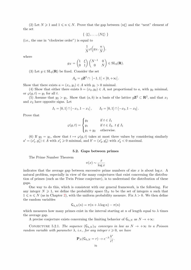
(2) Let N > 1 and 1 6 n 6 N . Prove that the gap between 〈nξ〉 and the “next” element ofthe set
〈ξ〉, . . . , 〈Nξ〉
(i.e., the one in “clockwise order”) is equal to
1
Nϕ(gN ,
n
N
),
where
gN =
(1 ξ0 1
)(N−1 0
0 N
)∈ SL2(R).
(3) Let g ∈ SL2(R) be fixed. Consider the set
Ag = gZ2 ∩ ]−1, 1[× ]0,+∞[ .
Show that there exists a = (x1, y1) ∈ A with y1 > 0 minimal.(4) Show that either there exists b = (x2, y2) ∈ A, not proportional to a, with y2 minimal,
or ϕ(g, t) = y1 for all t.(5) Assume that y2 > y1. Show that (a, b) is a basis of the lattice gZ2 ⊂ R2, and that x1
and x2 have opposite signs. Let
I1 = ]0, 1] ∩ ]−x1, 1− x1] , I2 = ]0, 1] ∩ ]−x2, 1− x2] .
Prove that
ϕ(g, t) =
y2 if t ∈ I1
y1 if t ∈ I2, t /∈ I1
y1 + y2 otherwise.
(6) If y2 = y1, show that t 7→ ϕ(g, t) takes at most three values by considering similarlya′ = (x′1, y
′1) ∈ A with x′1 > 0 minimal, and b′ = (x′2, y
′2) with x′2 < 0 maximal.
5.2. Gaps between primes
The Prime Number Theorem
π(x) ∼ x
log x
indicates that the average gap between successive prime numbers of size x is about log x. Anatural problem, especially in view of the many conjectures that exist concerning the distribu-tion of primes (such as the Twin Prime conjecture), is to understand the distribution of thesegaps.
One way to do this, which is consistent with our general framework, is the following. Forany integer N > 1, we define the probability space ΩN to be the set of integers n such that1 6 n 6 N (as in Chapter 2), with the uniform probability measure. Fix λ > 0. We then definethe random variables
Gλ,N (n) = π(n+ λ log n)− π(n)
which measures how many primes exist in the interval starting at n of length equal to λ timesthe average gap.
A precise conjecture exists concerning the limiting behavior of Gλ,N as N → +∞:
Conjecture 5.2.1. The sequence (Gλ,N )N converges in law as N → +∞ to a Poissonrandom variable with parameter λ, i.e., for any integer r > 0, we have
PN (Gλ,N = r)→ e−λλr
r!.
70
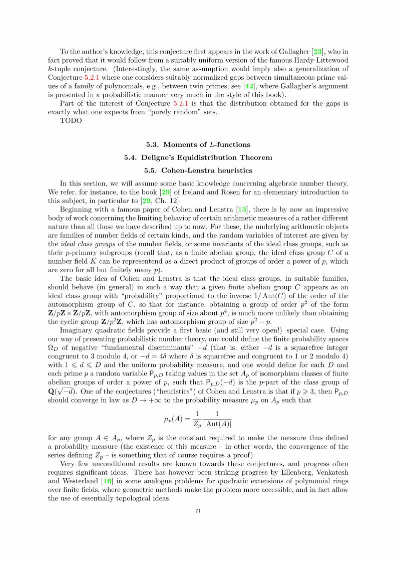
To the author’s knowledge, this conjecture first appears in the work of Gallagher [23], who infact proved that it would follow from a suitably uniform version of the famous Hardy-Littewoodk-tuple conjecture. (Interestingly, the same assumption would imply also a generalization ofConjecture 5.2.1 where one considers suitably normalized gaps between simultaneous prime val-ues of a family of polynomials, e.g., between twin primes; see [42], where Gallagher’s argumentis presented in a probabilistic manner very much in the style of this book).
Part of the interest of Conjecture 5.2.1 is that the distribution obtained for the gaps isexactly what one expects from “purely random” sets.
TODO
5.3. Moments of L-functions
5.4. Deligne’s Equidistribution Theorem
5.5. Cohen-Lenstra heuristics
In this section, we will assume some basic knowledge concerning algebraic number theory.We refer, for instance, to the book [29] of Ireland and Rosen for an elementary introduction tothis subject, in particular to [29, Ch. 12].
Beginning with a famous paper of Cohen and Lenstra [13], there is by now an impressivebody of work concerning the limiting behavior of certain arithmetic measures of a rather differentnature than all those we have described up to now. For these, the underlying arithmetic objectsare families of number fields of certain kinds, and the random variables of interest are given bythe ideal class groups of the number fields, or some invariants of the ideal class groups, such astheir p-primary subgroups (recall that, as a finite abelian group, the ideal class group C of anumber field K can be representend as a direct product of groups of order a power of p, whichare zero for all but finitely many p).
The basic idea of Cohen and Lenstra is that the ideal class groups, in suitable families,should behave (in general) in such a way that a given finite abelian group C appears as anideal class group with “probability” proportional to the inverse 1/Aut(C) of the order of theautomorphism group of C, so that for instance, obtaining a group of order p2 of the formZ/pZ×Z/pZ, with automorphism group of size about p4, is much more unlikely than obtainingthe cyclic group Z/p2Z, which has automorphism group of size p2 − p.
Imaginary quadratic fields provide a first basic (and still very open!) special case. Usingour way of presenting probabilistic number theory, one could define the finite probability spacesΩD of negative “fundamental discriminants” −d (that is, either −d is a squarefree integercongruent to 3 modulo 4, or −d = 4δ where δ is squarefree and congruent to 1 or 2 modulo 4)with 1 6 d 6 D and the uniform probability measure, and one would define for each D andeach prime p a random variable Pp,D taking values in the set Ap of isomorphism classes of finiteabelian groups of order a power of p, such that Pp,D(−d) is the p-part of the class group of
Q(√−d). One of the conjectures (“heuristics”) of Cohen and Lenstra is that if p > 3, then Pp,D
should converge in law as D → +∞ to the probability measure µp on Ap such that
µp(A) =1
Zp
1
|Aut(A)|
for any group A ∈ Ap, where Zp is the constant required to make the measure thus defineda probability measure (the existence of this measure – in other words, the convergence of theseries defining Zp – is something that of course requires a proof).
Very few unconditional results are known towards these conjectures, and progress oftenrequires significant ideas. There has however been striking progress by Ellenberg, Venkateshand Westerland [16] in some analogue problems for quadratic extensions of polynomial ringsover finite fields, where geometric methods make the problem more accessible, and in fact allowthe use of essentially topological ideas.
71
5.6. Ratner theory
Although all the results that we have described up to now are beautiful and important,maybe the most remarkably versatile tool that can be considered to lie within our chosen contextis Ratner theory, named after the fundamental work of M. Ratner [59]. We lack the expertiseto present anything more than a few selected statements of applications of this theory; we referto the survey of E. Ghys [24] and to the book of Morris [54] for an introduction (Section 1.4of that book list more applications of Ratner Theory), and to that of Einsiedler and Ward [14]for background results on ergodic theory and dynamical systems (some of which also haveremarkable applications in number theory, and are very much in the spirit of these notes).
We now illustrate the remarkable consequences of this theory with the beautiful result ofElkies and McMullen [15] which was alrady mentioned in Section 5.1. We consider the sequenceof fractional parts of
√n for n > 1 (viewed as elements of R/Z). As in the previous section,
for any integer N > 1, we define the space ΩN to be the set of connected components ofR/Z 〈1〉, . . . , 〈
√N〉, with uniform probability measure, and we define random variables on
ΩN by
GN (I) = N length(I).
Elkies and McMullen found the limiting distribution of GN as N → +∞. It is a very non-genericprobability measure on R!
Theorem 5.6.1 (Elkies–McMullen). As N → +∞, the random variables GN converge in lawto a random variable on [0,+∞[ with probability law µEM = 6
π2 f(x)dx, where f is continuous,
analytic on the intervals [0, 1/2], [1/2, 2] and [2,+∞[, is not of class C3, and satisfies f(x) = 1if 0 6 x 6 1/2.
This is [15, Th. 1.1]. The restriction of the density f to the two intervals [1/2, 2] and[2,+∞[ can be written down explicitly and it is an “elementary” function. For instance, if1/2 6 x 6 2, then let r = 1
2x−1 and
ψ(r) = arctan( 2r − 1√
4r − 1
)− arctan
( 1√4r − 1
);
we then have
f(x) =2
3(4r − 1)3/2ψ(r) + (1− 6r) log r + 2r − 1
(see [15, (3.53)]).We give the barest outline of the proof, in order to simply point out what kind of results are
meant by Ratner Theory. The paper of Elkies and McMullen also gives a detailed and highlyreadable introduction to this area.
The proof studies the gap distribution by means of the function LN defined for x ∈ R/Z sothat LN (x) is the measure of the gap interval containing x (with LN (x) = 0 if x is one of the
boundary points of the gap intervals for 〈√
1〉, . . . , 〈√N〉). We can then check that for t ∈ R,
the total measure in R/Z of the points lying in an interval of length < t, which is equal to theLebesgue measure
µ(x ∈ R/Z | LN (x) < t),is given by ∫ t
0td(PN (GN < t)) = tPN (GN < t)−
∫ t
0PN (GN < t)dt.
Concretely, this means that it is enough to understand the limiting behavior of LN in orderto understand the limit gap distribution. Note that there is nothing special about the specificsequence considered in that part of the argument.
Fix t > 0. The key insight that leads to questions involving Ratner theory is that if N is asquare of an integer, then the probability
µ(x ∈ R/Z | LN (x) < t)72
can be shown (asymptotically as N → +∞) to be very close to the probability that a certainaffine lattice ΛN,x in R2 intersects the triangle ∆t with vertices (0, 0), (1, 0) and (0, 2t) (witharea t). The lattice has the form ΛN,x = gN,x ·Z2, for some (fairly explicit) affine transformationgN,t.
Let ASL2(R) be the group of affine transformations
z 7→ z0 + g(z)
of R2 whose linear part g ∈ GL2(R) has determinant 1, and ASL2(Z) the subgroup of thoseaffine transformations of determinant 1 where both the translation term z0 and the linear parthave coefficients in Z. Then the lattices ΛN,x can be interpreted as elements of the quotientspace
M = ASL2(Z)\ASL2(R)
which parameterizes affine lattices Λ ⊂ R2 with R2/Λ of area 1. This space admits a uniqueprobability measure µ that is invariant under the right action of ASL2(R) by multiplication.
Now we have, for each N > 1, a probability measure µN on M , namely the law of therandom variable R/Z → M defined by x 7→ ΛN,x. What Ratner Theory provides is a verypowerful set of tools to prove that certain probability measures on M (or on similar spacesconstructed with groups more general than ASL2(R) and suitable quotients) are equal to thecanonical measure µ. This is applied, essentially, to all possible limits of subsequences of (µN ),to show that these must coincide with µ, which leads to the conclusion that the whole sequenceconverges in law to µ. It then follows that
µ(x ∈ R/Z | LN (x) < t)→ µ(Λ ∈M | M ∩∆t 6= ∅).The gives, in principle, an explicit form of the gap distribution. To compute it exactly is an“exercise” in euclidean geometry – which is by no means easy!
73
APPENDIX A
Complex analysis
In Chapter 3, we use a number of facts of complex analysis which are not necessarily includedin most introductory graduate courses. We review them here, and give some details of the proofs(when they are sufficiently elementary and enlightening) or detailed references.
A.1. Mellin transform
The Mellin transform is a multiplicative analogue of the Fourier transform, to which it canindeed in principle be reduced. We consider it only in simple cases. Let
ϕ : [0,+∞[−→ C
be a continuous function that decays faster than any polynomial at infinity (for instance, afunction with compact support). Then the Mellin transform ϕ of ϕ is the holomorphic functiondefined by the integral
ϕ(s) =
∫ +∞
0ϕ(x)xs
dx
x,
for all those s ∈ C for which the integral makes sense, which under our assumption includes allcomplex numbers with Re(s) > 0.
The basic properties of the Mellin transform that are relevant for us are summarized in thenext proposition:
Proposition A.1.1. Let ϕ : [0,+∞[−→ C be smooth and assume that it and all its deriva-tives decay faster than any polynomial at infinity.
(1) The Mellin transform ϕ extends to a meromorphic function on Re(s) > −1, with atmost a simple pole at s = 0 with residue ϕ(0).
(2) For any real numbers −1 < A < B, the Mellin transform has rapid decay in the stripA 6 Re(s) 6 B, in the sense that for any integer k > 1, there exists a constant Ck > 0 suchthat
|ϕ(s)| 6 Ck(1 + |t|)−k
for all s = σ + it with A 6 σ 6 B and |t| > 1.(3) For any σ > 0 and any x > 0, we have the Mellin inversion formula
ϕ(x) =1
2iπ
∫(σ)ϕ(s)x−sds.
In the last formula, the notation∫
(σ)(· · · )ds refers to an integral over the vertical line
Re(s) = σ, oriented upward.
Proof. (1) We integrate by parts in the definition of ϕ(s) for Re(s) > 0, and obtain
ϕ(s) =[ϕ(x)
xs
s
]+∞
0− 1
s
∫ +∞
0ϕ′(x)xs+1dx
x= −1
s
∫ +∞
0ϕ′(x)xs+1dx
x
since ϕ and ϕ′ decay faster than any polynomial at∞. It follows that ψ(s) = sϕ(s) is holomor-phic for Re(s) > −1, and hence that ϕ(s) is meromorphic in this region. Since
ψ(0) = −∫ +∞
0ϕ′(x)dx = ϕ(0),
it follows that there is at most a simple pole with residue ϕ(0) at s = 0.
74
(2) Iterating the integration by parts k > 2 times, we obtain for Re(s) > −1 the relation
ϕ(s) =(−1)k
s(s+ 1) · · · (s+ k)
∫ +∞
0ϕ(k)(x)xs+k
dx
x.
Hence for A 6 σ 6 B and |t| > 1 we obtain the bound
|ϕ(s)| 1
(1 + |t|)k
∫ +∞
0|ϕ(k)(x)|xB+k dx
x 1
(1 + |t|)k.
(3) We interpret ϕ(s), for s = σ + it with σ > 0 fixed, as a Fourier transform: we have
ϕ(s) =
∫ +∞
0ϕ(x)xσxit
dx
x=
∫Rϕ(ey)eσyeiytdy,
which shows that t 7→ ϕ(σ + it) is the Fourier transform (with the above normalization) of thefunction g(y) = ϕ(ey)eσy. Note that g is smooth, and tends to zero very rapidly at infinity (fory → −∞, this is because ϕ is bounded close to 0, but eσy then tends exponentially fast to 0).Therefore the Fourier inversion formula holds, and for any y ∈ R, we obtain
ϕ(ey)eσy =1
2π
∫Rϕ(σ + it)e−itydt.
Putting x = ey, this translates to
ϕ(x) =1
2π
∫Rϕ(σ + it)x−σ−itdt =
1
2iπ
∫(σ)ϕ(s)x−sds.
One of the most important functions of analysis is classically defined as a Mellin transform.This is the Gamma function of Euler, which is essentially the Mellin transform of the exponentialfunction, or more precisely of exp(−x). In other words, we have
Γ(s) =
∫ +∞
0e−xxs
dx
x
for all complex numbers s such that Re(s) > 0. Proposition A.1.1 shows that Γ extends to ameromorphic function on Re(s) > −1, with a simple pole at s = 0 with residue 1. In fact, muchmore is true:
Proposition A.1.2. The function Γ(s) extends to a meromorphic function on C with onlysimples poles at s = −k for all integers k > 0, with residue (−1)k/k!. It satisfies
Γ(s+ 1) = sΓ(s)
for all s ∈ C, with the obvious meaning if s or s+ 1 is a pole, and in particular we have
Γ(n) = (n− 1)!
for all integers n > 0.
Proof. It suffices to prove that Γ(s+1) = sΓ(s) for Re(s) > 0. Indeed, this formula proves,by induction on k > 1, that Γ has an analytic continuation to Re(s) > −k, with a simple poleat −k + 1, where the residue r−k+1 satisfies
r−k+1 =r−k+2
−k + 1.
This easily gives every statement in the proposition. And the formula we want is just a simpleintegration by parts away:
Γ(s+ 1) =
∫ +∞
0e−xxsdx =
[−e−xxs
]+∞
0+ s
∫ +∞
0e−xxs−1dx = sΓ(s).
75
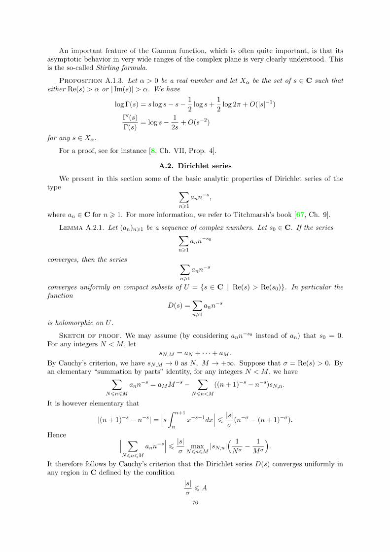
An important feature of the Gamma function, which is often quite important, is that itsasymptotic behavior in very wide ranges of the complex plane is very clearly understood. Thisis the so-called Stirling formula.
Proposition A.1.3. Let α > 0 be a real number and let Xα be the set of s ∈ C such thateither Re(s) > α or | Im(s)| > α. We have
log Γ(s) = s log s− s− 1
2log s+
1
2log 2π +O(|s|−1)
Γ′(s)
Γ(s)= log s− 1
2s+O(s−2)
for any s ∈ Xα.
For a proof, see for instance [8, Ch. VII, Prop. 4].
A.2. Dirichlet series
We present in this section some of the basic analytic properties of Dirichlet series of thetype ∑
n>1
ann−s,
where an ∈ C for n > 1. For more information, we refer to Titchmarsh’s book [67, Ch. 9].
Lemma A.2.1. Let (an)n>1 be a sequence of complex numbers. Let s0 ∈ C. If the series∑n>1
ann−s0
converges, then the series ∑n>1
ann−s
converges uniformly on compact subsets of U = s ∈ C | Re(s) > Re(s0). In particular thefunction
D(s) =∑n>1
ann−s
is holomorphic on U .
Sketch of proof. We may assume (by considering ann−s0 instead of an) that s0 = 0.
For any integers N < M , letsN,M = aN + · · ·+ aM .
By Cauchy’s criterion, we have sN,M → 0 as N, M → +∞. Suppose that σ = Re(s) > 0. Byan elementary “summation by parts” identity, for any integers N < M , we have∑
N6n6M
ann−s = aMM
−s −∑
N6n<M
((n+ 1)−s − n−s)sN,n.
It is however elementary that
|(n+ 1)−s − n−s| =∣∣∣s ∫ n+1
nx−s−1dx
∣∣∣ 6 |s|σ
(n−σ − (n+ 1)−σ).
Hence ∣∣∣ ∑N6n6M
ann−s∣∣∣ 6 |s|
σmax
N6n6M|sN,n|
( 1
Nσ− 1
Mσ
).
It therefore follows by Cauchy’s criterion that the Dirichlet series D(s) converges uniformly inany region in C defined by the condition
|s|σ6 A
76
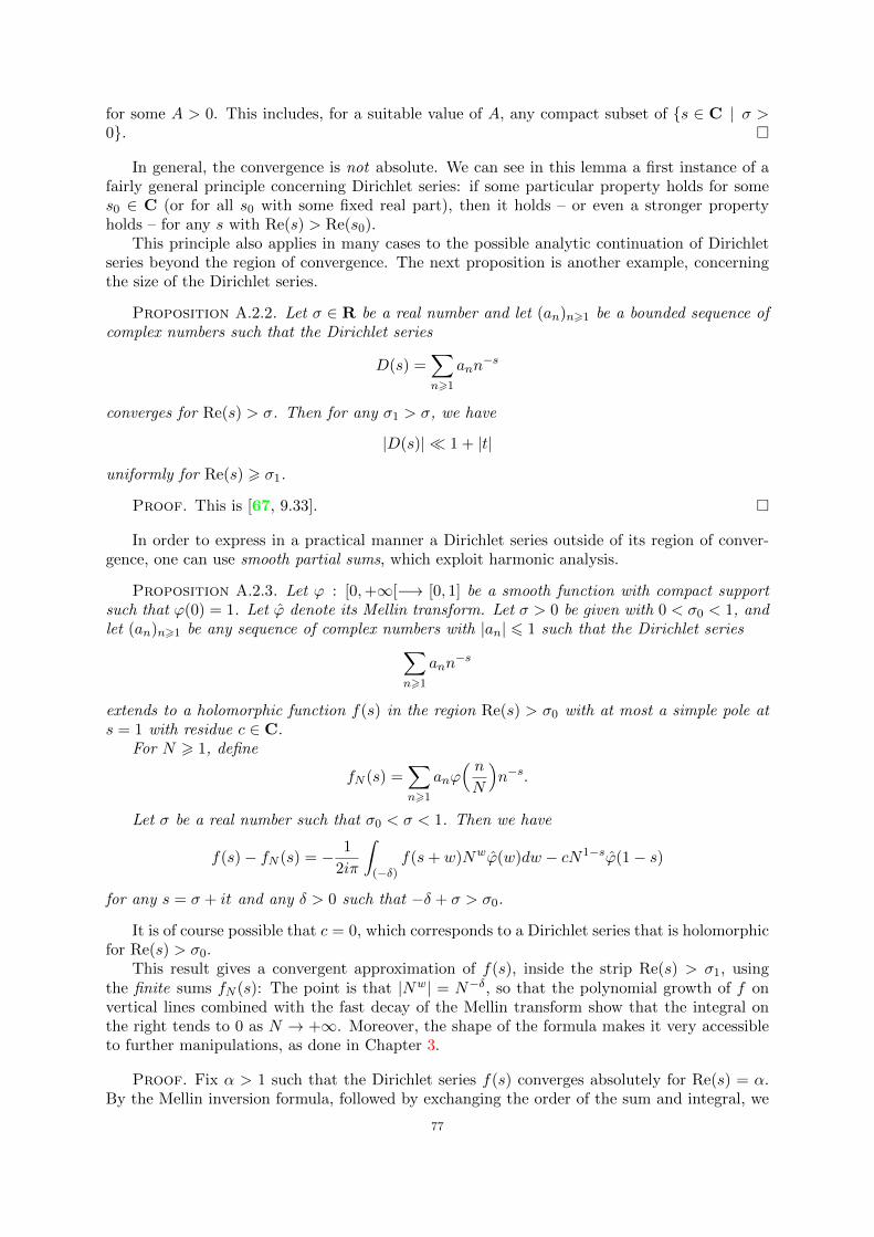
for some A > 0. This includes, for a suitable value of A, any compact subset of s ∈ C | σ >0.
In general, the convergence is not absolute. We can see in this lemma a first instance of afairly general principle concerning Dirichlet series: if some particular property holds for somes0 ∈ C (or for all s0 with some fixed real part), then it holds – or even a stronger propertyholds – for any s with Re(s) > Re(s0).
This principle also applies in many cases to the possible analytic continuation of Dirichletseries beyond the region of convergence. The next proposition is another example, concerningthe size of the Dirichlet series.
Proposition A.2.2. Let σ ∈ R be a real number and let (an)n>1 be a bounded sequence ofcomplex numbers such that the Dirichlet series
D(s) =∑n>1
ann−s
converges for Re(s) > σ. Then for any σ1 > σ, we have
|D(s)| 1 + |t|
uniformly for Re(s) > σ1.
Proof. This is [67, 9.33].
In order to express in a practical manner a Dirichlet series outside of its region of conver-gence, one can use smooth partial sums, which exploit harmonic analysis.
Proposition A.2.3. Let ϕ : [0,+∞[−→ [0, 1] be a smooth function with compact supportsuch that ϕ(0) = 1. Let ϕ denote its Mellin transform. Let σ > 0 be given with 0 < σ0 < 1, andlet (an)n>1 be any sequence of complex numbers with |an| 6 1 such that the Dirichlet series∑
n>1
ann−s
extends to a holomorphic function f(s) in the region Re(s) > σ0 with at most a simple pole ats = 1 with residue c ∈ C.
For N > 1, define
fN (s) =∑n>1
anϕ( nN
)n−s.
Let σ be a real number such that σ0 < σ < 1. Then we have
f(s)− fN (s) = − 1
2iπ
∫(−δ)
f(s+ w)Nwϕ(w)dw − cN1−sϕ(1− s)
for any s = σ + it and any δ > 0 such that −δ + σ > σ0.
It is of course possible that c = 0, which corresponds to a Dirichlet series that is holomorphicfor Re(s) > σ0.
This result gives a convergent approximation of f(s), inside the strip Re(s) > σ1, usingthe finite sums fN (s): The point is that |Nw| = N−δ, so that the polynomial growth of f onvertical lines combined with the fast decay of the Mellin transform show that the integral onthe right tends to 0 as N → +∞. Moreover, the shape of the formula makes it very accessibleto further manipulations, as done in Chapter 3.
Proof. Fix α > 1 such that the Dirichlet series f(s) converges absolutely for Re(s) = α.By the Mellin inversion formula, followed by exchanging the order of the sum and integral, we
77
have
fN (s) =∑n>1
ann−s × 1
2iπ
∫(α)
Nwn−wϕ(w)dw
=1
2iπ
∫(−δ)
(∑n>1
ann−s−w
)Nwϕ(w)dw
=1
2iπ
∫(−δ)
f(s+ w)Nwϕ(w)dw,
where the absolute convergence justifies the exchange of sum and integral.Now consider some T > 1, and some δ such that 0 < δ < 1. Let RT be the rectangle in
C with sides [α− iT, α + iT ], [α + iT,−δ + iT ], [−δ + iT,−δ − T ], [−δ − iT, α− iT ], orientedcounterclockwise. Inside this rectangle, the function
w 7→ f(s+ w)Nwϕ(w)
is meromorphic. It has a simple pole at w = 0, by our choice of δ and the properties of theMellin transform of ϕ given by Proposition A.1.1, where the residue at w = 0 is ϕ(0)f(s) = f(s),again by Proposition A.1.1. It may (if c 6= 0) also have a simple pole at w = 1− s, with residueequal to cN1−sϕ(1− s).
Cauchy’s Integral theorem therefore implies that
fN (s) = f(s) +1
2iπ
∫RT
f(s+ w)Nwϕ(w)dw + cN1−sϕ(1− s).
Now we let T → +∞. Our assumptions imply that w 7→ f(s + w) has polynomial growth onthe strip −δ 6 Re(w) 6 α, and therefore the fast decay of ϕ (Proposition A.1.1 again) showsthat the contribution of the two horizontal segments to the integral along RT tends to 0 asT → +∞. Taking into account orientation, we get
f(s)− fN (s) = − 1
2iπ
∫(−δ)
f(s+ w)Nwϕ(w)dw − cN1−sϕ(1− s),
as claimed.
We also recall that formula for the product of two Dirichlet series, which involves the so-called Dirichlet convolution.
Proposition A.2.4. Let (a(n))n>1 and (b(n))n>1 be sequences of complex numbers. Forany s ∈ C such that the Dirichlet series
A(s) =∑n>1
a(n)n−s, B(s) =∑n>1
b(n)n−s,
converge absolutely, we have
A(s)B(s) =∑n>1
c(n)n−s,
where
c(n) =∑d|nd>1
a(d)b(nd
).
We will denote c(n) = (a ? b)(n), and often abbreviate the definition by writing
(a ? b)(n) =∑d|n
a(d)b(nd
), or (a ? b)(n) =
∑de=n
a(d)b(e).
78
Proof. Formally, this is quite clear:
A(s)B(s) =(∑n>1
a(n)n−s)(∑
n>1
b(m)m−s)
=∑m,n>1
a(n)b(m)(nm)−s =∑k>1
k−s( ∑mn=k
a(n)b(m))
= C(s),
and the assumptions are sufficient to allow us to rearrange the double series so that thesemanipulations are valid.
A.3. Density of certain sets of holomorphic functions
Let D be a non-empty open disc in C and D its closure. We denote by H(D) the Banachspace of all continuous functions f : D −→ C which are holomorphic in D, with the norm
‖f‖∞ = supz∈D|f(z)|.
We also denote by C(K) the Banach space of continuous functions on a compact space K,also with the norm
‖f‖∞ = supx∈K|f(x)|
(so that there is no risk of confusion if K = D and we apply this to a function that alsobelongs to H(D)). We denote by C(K)′ the dual of C(K), namely the space of continuouslinear functionals C(K) −→ C. An element µ ∈ C(K)′ can also be interpreted as a complexmeasure on K (by the Riesz-Markov Theorem, see e.g. [18, Th. 7.17]), and in this interpretationone would write
µ(f) =
∫Kf(x)dµ(x).
Theorem A.3.1. Let D be as above. Let (fn)n>1 be a sequence of elements of H(D) with∑n>1
‖fn‖2∞ < +∞.
Let X be the set of sequences (αn) of complex numbers with |αn| = 1 such that the series∑n>1
αnfn
converges in H(D).Assume that X is not empty and that, for any continuous linear functional µ ∈ C(D)′ such
that
(A.1)∑n>1
|µ(fn)| < +∞,
the Laplace transform of µ is identically 0. Then for any N > 1, the set of series∑n>N
αnfn
for (αn) in X is dense in H(D).
Here, the Laplace transform of µ is defined by
g(z) = µ(w 7→ ewz)
for z ∈ C. In the interpretation of µ as a complex measure, which can be viewed as a complexmeasure on C that is supported on D, one would write
g(z) =
∫Cewzdµ(w).
79
Proof. This result is proved, for instance, in [1, Lemma 5.2.9], except that only the caseN = 1 is considered. However, if the assumptions hold for (fn)n>1, they hold equally for(fn)n>N , hence the general case follows.
We will use the last part of the following lemma as a criterion to establish that the Laplacetransform is zero in certain circumstances.
Lemma A.3.2. Let K be a complex subset of C and µ ∈ C(K)′ a continuous linear func-tional. Let
g(z) =
∫ewzdµ(z) = µ(w 7→ ewz)
be its Laplace transform.(1) The function g is an entire function on C, i.e., it is holomorphic on C.(2) We have
lim sup|z|→+∞
log |g(z)||z|
< +∞.
(3) If g 6= 0, then
lim supr→+∞
log |g(r)|r
> infz∈K
Re(z).
Proof. (1) Let z ∈ C be fixed. For h 6= 0, we have
g(z + h)− g(z)
h= µ(fh)
where fh(w) = (ew(z+h) − ewz)/h. We have
fh(w)→ wewz
as h→ 0, and the convergence is uniform on K. Hence we get
g(z + h)− g(z)
h−→ µ(w 7→ wewz),
which shows that g is holomorphic at z with derivative µ(w 7→ wewz). Since z is arbitrary, thismeans that g is entire.
(2) We have
|g(z)| 6 ‖µ‖ ‖w 7→ ewz‖∞ 6 ‖µ‖e|z|M
where M = supw∈K |w|, and therefore
lim sup|z|→+∞
log |g(z)||z|
6M < +∞.
(3) This is proved, for instance, in [1, Lemma 5.2.2], using relatively elementary propertiesof entire functions satisfying growth conditions such as those in (2).
Finally, we will use the following theorem of Bernstein, extending a result of Polya.
Theorem A.3.3. Let g : C −→ C be an entire function such that
lim sup|z|→+∞
log |g(z)||z|
< +∞.
Let (rk) be a sequence of positive real numbers, and let α, β be real numbers such that(1) We have αβ < π;(2) We have
lim supy∈R|y|→+∞
log |g(iy)||y|
6 α.
(3) We have |rk − rl| |k − l| for all k, l > 1, and rk/k → β.
80
Then it follows that
lim supk→+∞
log |g(rk)|rk
= lim supr→+∞
log |g(r)|r
.
This is explained in Lemma [1, 5.2.3].
Example A.3.4. Taking g(z) = sin(πz), with α = 1, rn = nπ so that β = π, we see thatthe first condition is best possible.
We also use a relatively elementary lemma due to Hurwitz on zeros of holomorphic functions
Lemma A.3.5. Let D be a non-empty open disc in C. Let (fn) be a sequence of holomorphicfunctions in H(D). Assume fn converges to f in H(D). If fn(z) 6= 0 all n > 1 and z ∈ D, theneither f = 0 or f does not vanish on D.
Proof. We assume that f is not zero, and show that it has no zero in D. Let z0 ∈ D befixed, and let C be a circle of radius r > 0 centered at z0 and such that C ⊂ D. Since f isnon-zero in H(D), it is non-zero in the disc with boundary C, and by the maximum modulusprinciple, it is non-zero on C. In particular, we have δ = infz∈C |f(z)| > 0. For n large enough,we get
supz∈C|f(z)− fn(z)| < δ,
and then the relation f = f − fn + fn combined with Rouche’s Theorem (see, e.g., [67, 3.42])shows that f has the same number of zeros as fn in the disc bounded by C. This means thatf has no zeros there, and in particular that f(z0) 6= 0.
81
APPENDIX B
Probability
This Appendix summarizes the probabilistic notions that are most important in the notes.Although many readers will not need to be reminded of the basic definitions, they might stillrefer to it to check some easy probabilistic statements whose proof we have included here toavoid disrupting the arguments in the main part of the book. For convergence in law, we willrefer mostly to the book of Billingsley [4], and for random series and similar topics, to that ofLi and Queffelec [50].
B.1. Support of a measure
Let M be a topological space. If M is either second countable (i.e., there is basis of opensets that is countable) or compact, then any Radon measure µ on M has a well-defined closedsupport, denoted supp(µ), which is characterized by either of the following properties: (1) it isthe complement of the largest open set U , with respect to inclusion, such that µ(U) = 0; or (2)it is the set of those x ∈M such that, for any open neighborhood U of x, we have µ(U) > 0.
If X is a random variable with values in M , we will say that the support of X is the supportof the law of X, which is a probability measure on M .
We need the following elementary property of the support of a measure:
Lemma B.1.1. Let M and N be topological spaces that are each either second countable orcompact. Let µ be a probability measure on M , and let f : M −→ N be a continuous map. Thesupport of f∗(µ) is the closure of f(supp(µ)).
Proof. First, if y = f(x) for some x ∈ supp(µ), and if U is an open neighborhood of y, thenwe can find an open neighborhood V ⊂M of x such that f(V ) ⊂ U . Then (f∗µ)(V ) > µ(U) > 0.This shows that y belongs to the support of f∗µ. Since the support is closed, we deduce thatf(supp(µ)) ⊂ supp(f∗µ).
For the converse, let y ∈ N be in the support of f∗µ. For any open neighborhood U of y, wehave µ(f−1(U)) = (f∗µ)(U) > 0. This implies that f−1(U) ∩ supp(µ) is not empty, and sinceU is arbitrary, that y belongs to the closure of f(supp(µ)).
Recall that a family (Xi)i∈I of random variables, each taking possibly values in a differentmetric space Mi, is independent if, for any finite subset J ⊂ I, the joint distribution of (Xj)j∈Jis the measure on
∏Mj which is the product measure of the laws of the Xj ’s.
Lemma B.1.2. Let X = (Xi)i∈I be a finite family of random variables with values in atopological space M that is compact or second countable. Viewed as a random variable takingvalues in M I , we have
supp(X) =∏i∈I
supp(Xi).
Proof. If x = (xi) ∈M I , then an open neighborhood U of x contains a product set∏Ui,
where Ui is an open neighborhood of xi in M . Then we have
P(X ∈ U) > P(X ∈∏i
Ui) =∏i
P(Xi ∈ Ui)
by independence. If xi ∈ supp(Xi) for each i, then this is > 0, and hence x ∈ supp(X).
82
Conversely, if x ∈ supp(X), then for any j ∈ I, and any open neighborhood U of xj , the set
V = y = (yi)i∈I ∈M I | yj ∈ U ⊂M I
is an open neighborhood of x. Hence we have P(X ∈ V ) > 0, and since P(X ∈ V ) = P(Xi ∈ U),it follows that xj is in the support of Xj .
B.2. Convergence in law
Let M be a metric space. We view it as given with the Borel σ-algebra generated byopen sets, and we denote by Cb(M) the Banach space of bounded complex-valued continuousfunctions on M , with the norm
‖f‖∞ = supx∈M|f(x)|.
Given a sequence (µn) of probability measures on M , and a probability measure µ on M ,one says that µn converges weakly to µ if and only if, for any bounded and continuous functionf : M −→ R, we have
(B.1)
∫Mf(x)dµn(x) −→
∫Mf(x)dµ(x).
If (Ω,Σ,P) is a probability space and (Xn)n>1 is a sequence of M -valued random variables,and if X is an M -valued random variable, then one says that (Xn) converges in law to X if andonly if the measures Xn(P) converge weakly to X(P). If µ is a probability measure on M , thenwe will also say that Xn converges to µ if Xn(P) converge weakly to µ.
The probabilistic versions of (B.1) in those cases is that
(B.2) E(f(Xn)) −→ E(f(X)), E(f(Xn)) −→∫Mfdµ
for all functions f ∈ Cb(M).In both cases, the definition immediately implies the following very useful fact, which we
state in probabilistic language:
Proposition B.2.1. Let M be a metric space. Let (Xn) be a sequence of M -valued randomvariables such that Xn converges in law to a random variable X. For any metric space N andany continuous function ϕ : M → N , the N -valued random variables ϕ Xn converge in lawto ϕ X.
Proof. For any continuous and bounded function f : N −→ C, the composite f ϕ isbounded and continuous on M , and therefore convergence in law implies that
E(f(ϕ(Xn))) −→ E(f(ϕ(X))).
By definition, this formula, valid for all f , means that ϕ(Xn) converges in law to ϕ(X).
Another property that is useful in Chapter 3 is the following:
Proposition B.2.2. Let M be a complete separable metric space. Let (Xn) be a sequenceof M -valued random variables, and µ a probability measure on M . Then Xn converges in lawto µ if and only if we have
E(f(Xn))→∫Mf(x)dµ(x)
for all bounded Lipschitz functions f : M −→ C.
In other words, it is enough to prove the convergence property (B.2) for Lipschitz testfunctions.
83
Proof. A classical argument shows that convergence in law of (Xn) to µ is equivalent to
(B.3) µ(F ) > lim supn→+∞
P(Xn ∈ F )
for all closed subsets F of M (see, e.g., [4, Th. 2.1, (iii)]).However, the proof that convergence in law implies this property uses only Lipschitz test
functions f (see for instance [4, (ii)⇒(iii), p. 16, and (1.1), p. 8], where it is only stated thatthe relevant functions f are uniformly continuous, but this is shown by checking that they areLipschitz). Hence the assumption that (B.2) holds for Lipschitz functions implies (B.3) for allclosed subsets F , and consequently it implies convergence in law.
Corollary B.2.3. Let m > 1 be an integer. Let (Xn) and (Yn) be sequences of Rm-valuedrandom variables, let (αn) be a sequence in Rm and (βn) a sequence of real numbers. Assume
(1) The sequence (Xn) converges in law to a random variable X, and Xn is bounded by aconstant N > 0, independent of n.
(2) For all n, we have ‖Yn‖ 6 βn.(3) We have αn → (1, . . . , 1) and βn → 0 as n→ +∞.Then the sequence (αn · Xn + Yn)n converges in law to X in Rm, where · denotes the
componentwise product of vectors.1
Proof. Let f : Rm −→ C be a bounded Lipschitz continuous function, and C its Lipschitzconstant. For any n, we have
|E(f(αnXn + Yn))−E(f(X))| 6 |E(f(αnXn + Yn))−E(f(αnXn))|+ |E(f(αnXn))−E(f(Xn))|+ |E(f(Xn))−E(f(X))|.
The last term tends to 0 since Xn converges in law to X. The second is at most
C|αn − 1|E(‖Xn‖) 6 CN |αn − 1| → 0,
and the first is at mostC E(‖Yn‖) 6 Cβn → 0.
The result now follows from Proposition B.2.2.
A last general property is the following:
Lemma B.2.4. Let M be a second countable or compact topological space. Let (Xn) be asequence of M -valued random variables, defined on some probability spaces Ωn. Assume that(Xn) converges in law to some random variable X, and let N ⊂M be the support of the law ofX.
(1) For any x ∈ N and for any open neighborhood U of x, we have
lim infn→+∞
P(Xn ∈ U) > 0,
and in particular there exists some n > 1 and some ω ∈ Ωn such that Xn(ω) ∈ U .(2) For any x ∈M not belonging to N , there exists an open neighborhood U of x such that
lim supn→+∞
P(Xn ∈ U) = 0.
Proof. For (1), a standard equivalent form of convergence in law is that, for any open setU ⊂M , we have
lim infn→+∞
P(Xn ∈ U) > P(X ∈ U)
(see [4, Th. 2.1, (i) and (iv)]). If x ∈ N and U is an open neighborhood of x, then by definitionwe have P(X ∈ U) > 0, and therefore
lim infn→+∞
P(Xn ∈ U) > 0.
1 I.e., we have (a1, . . . , am) · (b1, . . . , bm) = (a1b1, . . . , ambm).
84
For (2), if x ∈ M is not in N , there exists an open neighborhood V of x such that P(X ∈V ) = 0. For some δ > 0, this neighborhood contains the closed ball C of radius δ around f ,and by [4, Th. 2.1., (i) and (iii)], we have
0 6 lim supp→+∞
P(Xn ∈ C) 6 P(X ∈ C) = 0,
hence the second assertion with U the open ball of radius δ.
We also recall an important definition that is a property of weak-compactness for a familyof probability measures (or random variables).
Definition B.2.5 (Tightness). Let M be a complete separable metric space. Let (µi)i∈Ibe a family of probability measures on M . One says that (µi) is tight if for any ε > 0, thereexists a compact subset K ⊂M such that µi(K) > 1− ε for all i ∈ I.
It is a non-obvious fact that a single probability measure on a complete separable metricspace is tight (see [4, Th. 1.3]).
B.3. Convergence in law in a finite-dimensional vector space
We will use two important criteria for convergence in law for random variables with valuesin a finite-dimensional real vector space V , which both amount to testing (B.1) for a restrictedset of functions. Another important criterion applies to variables with values in a compacttopological group, and is reviewed below in Section B.4.
The first result is valid in all cases, and is based on the Fourier transform. Given an integerm > 1 and a probability measure µ on Rm, recall that the characteristic function (or Fouriertransform) of µ is the function
ϕµ : Rm −→ C
defined by
ϕµ(t) =
∫Rm
eit·xdµ(x),
where t · x = t1x1 + · · · + tmxm is the standard inner-product. This is a continuous boundedfunction on Rm. For a random vector X with values in Rm, we denote by ϕX the characteristicfunction of X(P), namely
ϕX(t) = E(eit·X).
We state two (obviously equivalent) versions of P. Levy’s theorem for convenience:
Theorem B.3.1 (Levy). Let m > 1 be an integer.(1) Let (µn) be a sequence of probability measures on Rm, and let µ be a probability measure
on Rm. Then (µn) converges weakly to µ if and only if, for any t ∈ Rm, we have
ϕµn(t) −→ ϕµ(t)
as n→ +∞.(2) Let (Ω,Σ,P) be a probability space. Let (Xn)n>1 be Rm-valued random vectors on Ω,
and let X be an Rm-valued random vector. Then (Xn) converges in law to X if and only if, forall t ∈ Rm, we have
E(eit·Xn) −→ E(eit·X).
Remark B.3.2. In fact, the precise version of Levy’s Theorem does not require to know inadvance the limit of the sequence: if a sequence (µn) of probability measures is such that, forall t ∈ Rm, we have
ϕµn(t) −→ ϕ(t)
for some function ϕ, then one can show that ϕ is the characteristic function of a probabilitymeasure µ (and hence that µn converges weakly to µ). So, for instance, it is not necessary to
know beforehand that ϕ(t) = e−t2/2 is the characteristic function of a probability measure in
order to prove the Central Limit Theorem using Levy’s Criterion.
85

Lemma B.3.3. Let m > 1 be an integer. Let (Xn)n>1 be a sequence of random variableswith values in Rm on some probability space. Let (βn) be a sequence of positive real numberssuch that βn → 0 as n → +∞. If (Xn) converges in law to an Rm-valued random variable X,then for any sequence (Yn) of Rm-valued random variables such that ‖Xn − Yn‖∞ 6 βn for alln > 1, the random variables Yn converge to X.
Proof. We use Levy’s criterion. We fix t ∈ Rm and write
E(eit·Yn)−E(eit·X) = E(eit·Yn − eit·Xn) + E(eit·Xn − eit·X).
By Levy’s Theorem and our assumption on the convergence of the sequence(Xn), the secondterm on the right converges to 0 as n→ +∞. For the first, we can simply apply the dominatedconvergence theorem to derive the same conclusion: we have
‖(Xn − Yn)‖∞ 6 βn → 0
hence
eit·Yn − eit·Xn = eit·Yn(
1− eit·(Xn−Yn))→ 0
(pointwise) as n→ +∞. Moreover, we have∣∣∣eit·Yn − eit·Xn∣∣∣ 6 2
for all n > 1. Hence the dominated convergence theorem implies that the expectation E(eit·Yn−eit·Xn) converges to 0.
Levy’s Theorem applied once more allows us to conclude that (Yn) converges in law to X,as claimed.
The second convergence criterion is known as the method of moments. It is more restrictedthan Levy’s criterion, but is sometimes analytically more flexible.
Definition B.3.4 (Mild measure). Let µ be a probability measure on Rm. We will saythat µ is mild2 if the moments
Mk(µ) =
∫Rm
|x1|k1 · · · |xm|kmdµ(x1, . . . , xm)
exist for all tuples of non-negative integers k = (k1, . . . , km), and if there exists δ > 0 such thatthe power series ∑∑
ki>0
Mk(µ)zk11 · · · zkmmk1! · · · km!
converges in the region(z1, . . . , zm) ∈ Cm | |zi| 6 δ.
If X is a random variable, we will say as usual that a random vector X = (X1, . . . , Xm) ismild if its law X(P) is mild. The moments are then
Mk(X) = E(|X1|k1 · · · |Xm|km).
We again give two versions of the method of moments for weak convergence when the limitis mild:
Theorem B.3.5 (Method of moments). Let m > 1 be an integer.(1) Let (µn) be a sequence of probability measures on Rm such that all moments Mk(µn)
exist, and let µ be a probability measure on Rm. Assume that µ is mild. Then (µn) convergesweakly to µ if for any m-tuple k of non-negative integers, we have
Mk(µn) −→Mk(µ)
as n→ +∞.
2There doesn’t seem to be an especially standard name for this notion.
86
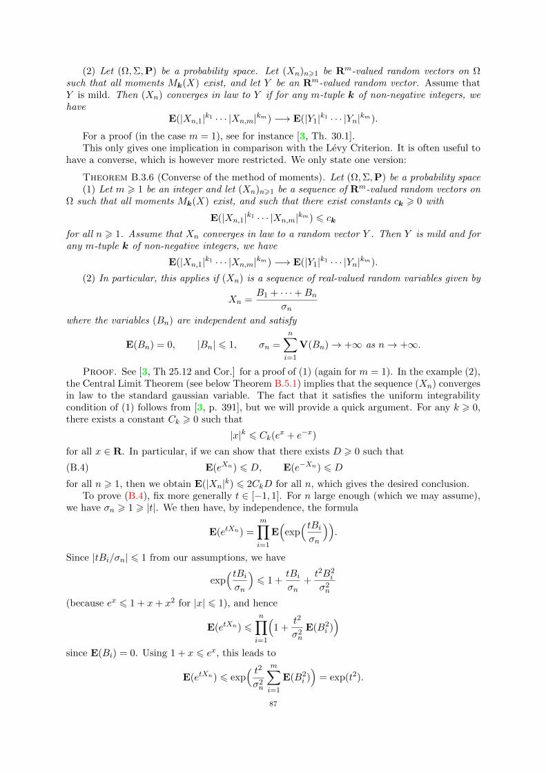
(2) Let (Ω,Σ,P) be a probability space. Let (Xn)n>1 be Rm-valued random vectors on Ωsuch that all moments Mk(X) exist, and let Y be an Rm-valued random vector. Assume thatY is mild. Then (Xn) converges in law to Y if for any m-tuple k of non-negative integers, wehave
E(|Xn,1|k1 · · · |Xn,m|km) −→ E(|Y1|k1 · · · |Yn|km).
For a proof (in the case m = 1), see for instance [3, Th. 30.1].This only gives one implication in comparison with the Levy Criterion. It is often useful to
have a converse, which is however more restricted. We only state one version:
Theorem B.3.6 (Converse of the method of moments). Let (Ω,Σ,P) be a probability space(1) Let m > 1 be an integer and let (Xn)n>1 be a sequence of Rm-valued random vectors on
Ω such that all moments Mk(X) exist, and such that there exist constants ck > 0 with
E(|Xn,1|k1 · · · |Xn,m|km) 6 ck
for all n > 1. Assume that Xn converges in law to a random vector Y . Then Y is mild and forany m-tuple k of non-negative integers, we have
E(|Xn,1|k1 · · · |Xn,m|km) −→ E(|Y1|k1 · · · |Yn|km).
(2) In particular, this applies if (Xn) is a sequence of real-valued random variables given by
Xn =B1 + · · ·+Bn
σn
where the variables (Bn) are independent and satisfy
E(Bn) = 0, |Bn| 6 1, σn =
n∑i=1
V(Bn)→ +∞ as n→ +∞.
Proof. See [3, Th 25.12 and Cor.] for a proof of (1) (again for m = 1). In the example (2),the Central Limit Theorem (see below Theorem B.5.1) implies that the sequence (Xn) convergesin law to the standard gaussian variable. The fact that it satisfies the uniform integrabilitycondition of (1) follows from [3, p. 391], but we will provide a quick argument. For any k > 0,there exists a constant Ck > 0 such that
|x|k 6 Ck(ex + e−x)
for all x ∈ R. In particular, if we can show that there exists D > 0 such that
(B.4) E(eXn) 6 D, E(e−Xn) 6 D
for all n > 1, then we obtain E(|Xn|k) 6 2CkD for all n, which gives the desired conclusion.To prove (B.4), fix more generally t ∈ [−1, 1]. For n large enough (which we may assume),
we have σn > 1 > |t|. We then have, by independence, the formula
E(etXn) =m∏i=1
E(
exp( tBiσn
)).
Since |tBi/σn| 6 1 from our assumptions, we have
exp( tBiσn
)6 1 +
tBiσn
+t2B2
i
σ2n
(because ex 6 1 + x+ x2 for |x| 6 1), and hence
E(etXn) 6n∏i=1
(1 +
t2
σ2n
E(B2i ))
since E(Bi) = 0. Using 1 + x 6 ex, this leads to
E(etXn) 6 exp( t2σ2n
m∑i=1
E(B2i ))
= exp(t2).
87
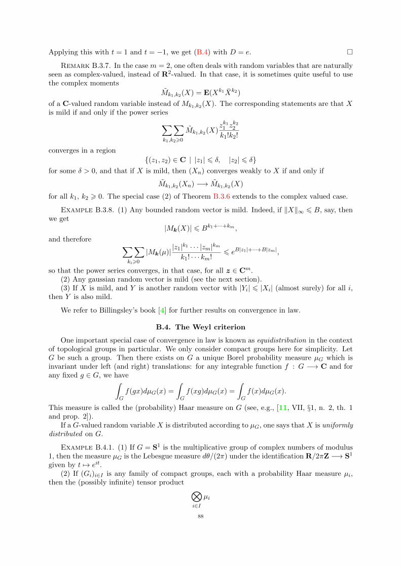
Applying this with t = 1 and t = −1, we get (B.4) with D = e.
Remark B.3.7. In the case m = 2, one often deals with random variables that are naturallyseen as complex-valued, instead of R2-valued. In that case, it is sometimes quite useful to usethe complex moments
Mk1,k2(X) = E(Xk1Xk2)
of a C-valued random variable instead of Mk1,k2(X). The corresponding statements are that Xis mild if and only if the power series∑∑
k1,k2>0
Mk1,k2(X)zk11 zk22
k1!k2!
converges in a region
(z1, z2) ∈ C | |z1| 6 δ, |z2| 6 δfor some δ > 0, and that if X is mild, then (Xn) converges weakly to X if and only if
Mk1,k2(Xn) −→ Mk1,k2(X)
for all k1, k2 > 0. The special case (2) of Theorem B.3.6 extends to the complex valued case.
Example B.3.8. (1) Any bounded random vector is mild. Indeed, if ‖X‖∞ 6 B, say, thenwe get
|Mk(X)| 6 Bk1+···+km ,
and therefore ∑∑ki>0
|Mk(µ)| |z1|k1 · · · |zm|kmk1! · · · km!
6 eB|z1|+···+B|zm|,
so that the power series converges, in that case, for all z ∈ Cm.(2) Any gaussian random vector is mild (see the next section).(3) If X is mild, and Y is another random vector with |Yi| 6 |Xi| (almost surely) for all i,
then Y is also mild.
We refer to Billingsley’s book [4] for further results on convergence in law.
B.4. The Weyl criterion
One important special case of convergence in law is known as equidistribution in the contextof topological groups in particular. We only consider compact groups here for simplicity. LetG be such a group. Then there exists on G a unique Borel probability measure µG which isinvariant under left (and right) translations: for any integrable function f : G −→ C and forany fixed g ∈ G, we have∫
Gf(gx)dµG(x) =
∫Gf(xg)dµG(x) =
∫Gf(x)dµG(x).
This measure is called the (probability) Haar measure on G (see, e.g., [11, VII, §1, n. 2, th. 1and prop. 2]).
If a G-valued random variable X is distributed according to µG, one says that X is uniformlydistributed on G.
Example B.4.1. (1) If G = S1 is the multiplicative group of complex numbers of modulus1, then the measure µG is the Lebesgue measure dθ/(2π) under the identification R/2πZ −→ S1
given by t 7→ eit.(2) If (Gi)i∈I is any family of compact groups, each with a probability Haar measure µi,
then the (possibly infinite) tensor product ⊗i∈I
µi
88
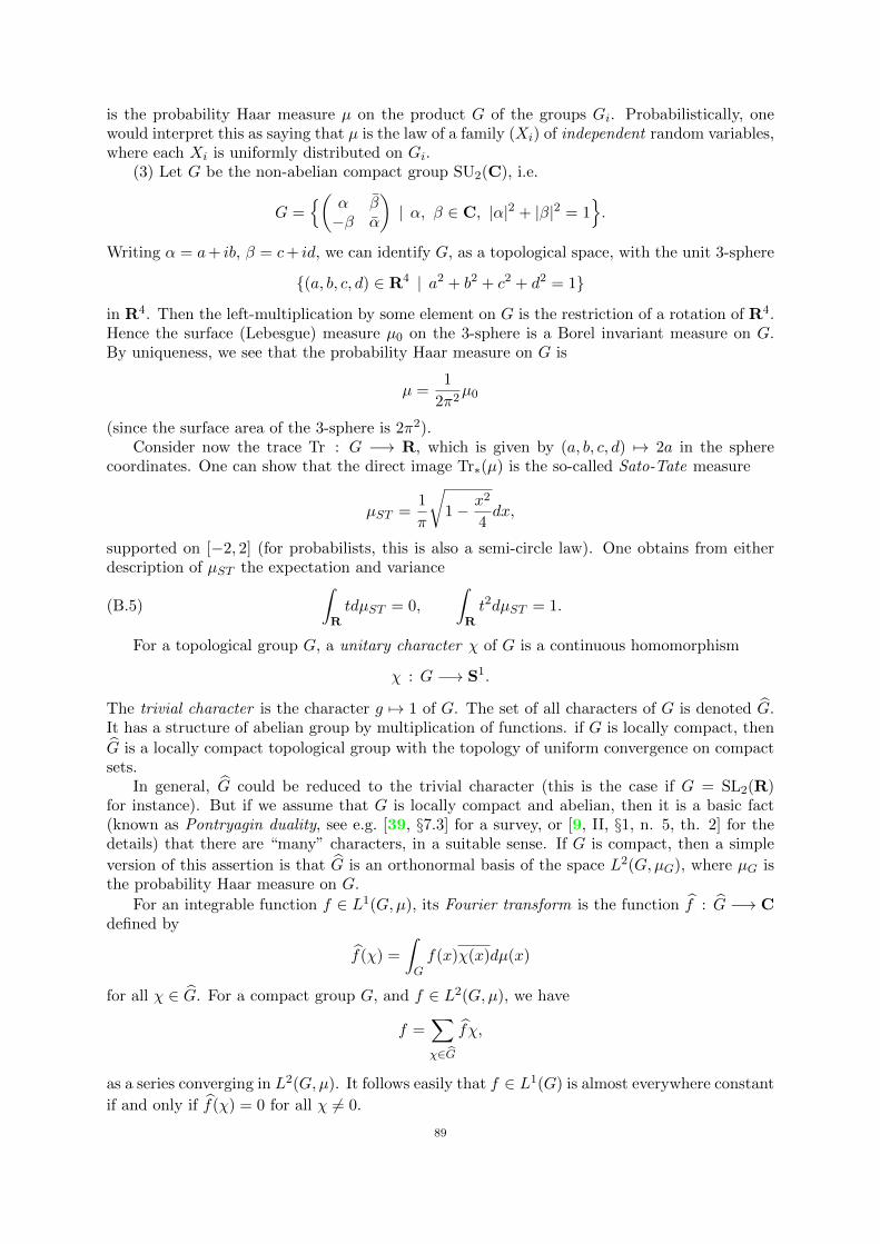
is the probability Haar measure µ on the product G of the groups Gi. Probabilistically, onewould interpret this as saying that µ is the law of a family (Xi) of independent random variables,where each Xi is uniformly distributed on Gi.
(3) Let G be the non-abelian compact group SU2(C), i.e.
G =(
α β−β α
)| α, β ∈ C, |α|2 + |β|2 = 1
.
Writing α = a+ ib, β = c+ id, we can identify G, as a topological space, with the unit 3-sphere
(a, b, c, d) ∈ R4 | a2 + b2 + c2 + d2 = 1
in R4. Then the left-multiplication by some element on G is the restriction of a rotation of R4.Hence the surface (Lebesgue) measure µ0 on the 3-sphere is a Borel invariant measure on G.By uniqueness, we see that the probability Haar measure on G is
µ =1
2π2µ0
(since the surface area of the 3-sphere is 2π2).Consider now the trace Tr : G −→ R, which is given by (a, b, c, d) 7→ 2a in the sphere
coordinates. One can show that the direct image Tr∗(µ) is the so-called Sato-Tate measure
µST =1
π
√1− x2
4dx,
supported on [−2, 2] (for probabilists, this is also a semi-circle law). One obtains from eitherdescription of µST the expectation and variance
(B.5)
∫RtdµST = 0,
∫Rt2dµST = 1.
For a topological group G, a unitary character χ of G is a continuous homomorphism
χ : G −→ S1.
The trivial character is the character g 7→ 1 of G. The set of all characters of G is denoted G.It has a structure of abelian group by multiplication of functions. if G is locally compact, then
G is a locally compact topological group with the topology of uniform convergence on compactsets.
In general, G could be reduced to the trivial character (this is the case if G = SL2(R)for instance). But if we assume that G is locally compact and abelian, then it is a basic fact(known as Pontryagin duality, see e.g. [39, §7.3] for a survey, or [9, II, §1, n. 5, th. 2] for thedetails) that there are “many” characters, in a suitable sense. If G is compact, then a simple
version of this assertion is that G is an orthonormal basis of the space L2(G,µG), where µG isthe probability Haar measure on G.
For an integrable function f ∈ L1(G,µ), its Fourier transform is the function f : G −→ Cdefined by
f(χ) =
∫Gf(x)χ(x)dµ(x)
for all χ ∈ G. For a compact group G, and f ∈ L2(G,µ), we have
f =∑χ∈G
fχ,
as a series converging in L2(G,µ). It follows easily that f ∈ L1(G) is almost everywhere constant
if and only if f(χ) = 0 for all χ 6= 0.
89
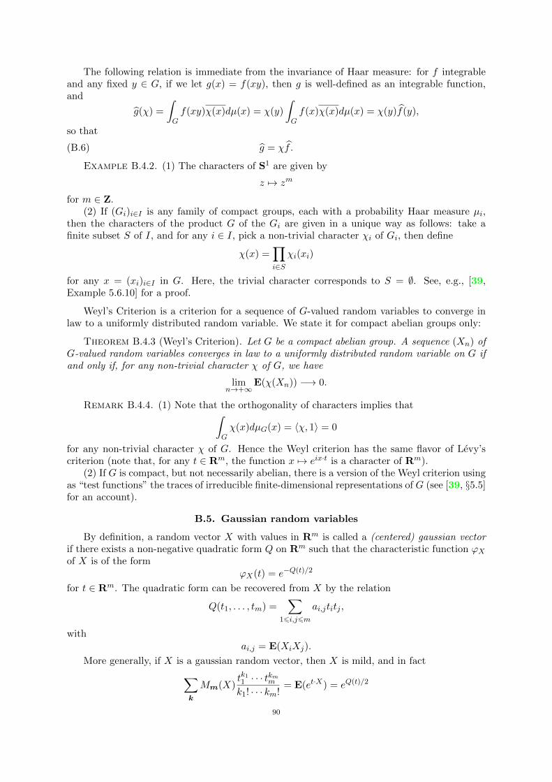
The following relation is immediate from the invariance of Haar measure: for f integrableand any fixed y ∈ G, if we let g(x) = f(xy), then g is well-defined as an integrable function,and
g(χ) =
∫Gf(xy)χ(x)dµ(x) = χ(y)
∫Gf(x)χ(x)dµ(x) = χ(y)f(y),
so that
(B.6) g = χf .
Example B.4.2. (1) The characters of S1 are given by
z 7→ zm
for m ∈ Z.(2) If (Gi)i∈I is any family of compact groups, each with a probability Haar measure µi,
then the characters of the product G of the Gi are given in a unique way as follows: take afinite subset S of I, and for any i ∈ I, pick a non-trivial character χi of Gi, then define
χ(x) =∏i∈S
χi(xi)
for any x = (xi)i∈I in G. Here, the trivial character corresponds to S = ∅. See, e.g., [39,Example 5.6.10] for a proof.
Weyl’s Criterion is a criterion for a sequence of G-valued random variables to converge inlaw to a uniformly distributed random variable. We state it for compact abelian groups only:
Theorem B.4.3 (Weyl’s Criterion). Let G be a compact abelian group. A sequence (Xn) ofG-valued random variables converges in law to a uniformly distributed random variable on G ifand only if, for any non-trivial character χ of G, we have
limn→+∞
E(χ(Xn)) −→ 0.
Remark B.4.4. (1) Note that the orthogonality of characters implies that∫Gχ(x)dµG(x) = 〈χ, 1〉 = 0
for any non-trivial character χ of G. Hence the Weyl criterion has the same flavor of Levy’scriterion (note that, for any t ∈ Rm, the function x 7→ eix·t is a character of Rm).
(2) If G is compact, but not necessarily abelian, there is a version of the Weyl criterion usingas “test functions” the traces of irreducible finite-dimensional representations of G (see [39, §5.5]for an account).
B.5. Gaussian random variables
By definition, a random vector X with values in Rm is called a (centered) gaussian vectorif there exists a non-negative quadratic form Q on Rm such that the characteristic function ϕXof X is of the form
ϕX(t) = e−Q(t)/2
for t ∈ Rm. The quadratic form can be recovered from X by the relation
Q(t1, . . . , tm) =∑
16i,j6m
ai,jtitj ,
withai,j = E(XiXj).
More generally, if X is a gaussian random vector, then X is mild, and in fact∑k
Mm(X)tk11 · · · tkmmk1! · · · km!
= E(et·X) = eQ(t)/2
90
for t ∈ Rm, so that the power series converges on all of Cm.For m = 1, this means that a random variable is a centered gaussian if and only if there
exists σ > 0 such that
ϕX(t) = e−σ2t/2,
and in fact we haveE(X2) = V(X) = σ2.
If σ = 1, then we say that X is a standard gaussian random variable, or a standard normalrandom variable. We then have
P(a < X < b) =1√2π
∫ b
ae−x
2/2dx
for all real numbers a < b.We will use the following simple version of the Central Limit Theorem:
Theorem B.5.1. Let B > 0 be a fixed real number. Let (Xn) be a sequence of independentreal-valued random variables with |Xn| 6 B for all n. Let
αn = E(Xn), βn = V(X2n).
Let σN > 0 be defined byσ2N = β1 + · · ·+ βN
for N > 1. If σN → +∞ as n→ +∞, then the random variables
YN =(X1 − α1) + · · ·+ (XN − αN )
σNconverge in law to a standard gaussian random variable.
Proof. Although this is a very simple case of the general Central Limit Theorem for sumsof independent random variables (indeed, even of Lyapunov’s well-known version), we give aproof using Levy’s criterion for convenience. First of all, we may assume that αn = 0 for all nby replacing Xn by Xn − αn (up to replacing B by 2B, since |αn| 6 B).
By independence of the variables (Xn), the characteristic function ϕN of YN is given by
ϕN (t) = E(eitYN ) =∏
16n6N
E(eitXn/σN )
for t ∈ R. We then have
E(eitXn/σN ) = ϕXn
( t
σN
)= 1− 1
2
( t
σN
)2E(X2
n) +O(( |t|
σN
)3E(|Xn|3)
).
Observe that with our assumption, we have
E(|Xn|3) 6 BE(X2n) = Bβn
and hence a simple computation shows that
ϕN (t) = exp( N∑n=1
log E(eitXn/σN ))
= exp(− t2
2σN
N∑n=1
βn +O(B|t|3σ3N
N∑n=1
βn
))= exp
(− t
2
2+O
(B|t|3σN
))−→ exp(−t2/2)
as N → +∞.
If one uses directly the method of moments to get convergence in law to a gaussian randomvariable, it is useful to know the values of their moments. We only state the one-dimensionaland the simplest complex case:
91
Proposition B.5.2. (1) Let X be a real-valued gaussian random variable with expectation0 and variance σ2. For k > 0, we have
E(Xk) =
0 if k is odd,
σk k!2k/2(k/2)!
= 1 · 3 · · · · (k − 1) if k is even.
(1) Let X be a complex-valued gaussian random variable with covariance matrix(σ 00 σ
)for some σ > 0. For k > 0 and l > 0, we have
E(XkX l) =
0 if k 6= l,
σk2kk! if k = l.
Exercise B.5.3. Prove this proposition.
B.6. Subgaussian random variables
Gaussian random variables have many remarkable properties. It is a striking fact that anumber of these, especially with respect to integrability properties, are shared by a much moregeneral class of random variables.
Definition B.6.1 (Subgaussian random variable). Let σ > 0 be a real number. A real-valued random variable X is σ2-subgaussian if we have
E(etX) 6 e−σ2t2/2
for all t ∈ R. A complex-valued random variable X is σ2-subgaussian if X = Y + iZ with Yand Z real-valued σ2-subgaussian random variables.
By definition, a gaussian random variable is therefore subgaussian. But there are manymore examples, in particular the random variables described in the next proposition.
Proposition B.6.2. (1) Let X be a complex-valued random variable and m > 0 a realnumber such that E(X) = 0 and |X| 6 m, for some real number m > 0. Then X is m2-subgaussian.
(2) Let X1 and X2 be independent random variables such that Xi is σ2i -subgaussian. Then
X1 +X2 is (σ21 + σ2
2)-subgaussian.
Proof. (1) We may assume that X is real-valued, and by considering m−1X instead of X,we may assume that |X| 6 1, and of course that X is not almost surely 0. In particular, thefunction ϕ(t) = E(etX) is well-defined, and ϕ(t) > 0 for all t ∈ R. Moreover, it is smooth on Rwith
ϕ′(t) = E(XetX), ϕ′′(t) = E(X2etX),
and in particularϕ(0) = 1, ϕ′(0) = E(X) = 0.
We now define f(t) = log(ϕ(t))− 12 t
2. The function f is also smooth and satisfies f(0) = f ′(0) =0. Moreover we have
f ′′(t) =ϕ′′(t)ϕ(t)− ϕ′(t)2 − ϕ(t)2
ϕ(t)2.
The formula for ϕ′′ and the condition |X| 6 1 imply that 0 6 ϕ′′(t) 6 ϕ(t) for all t ∈ R.Therefore
ϕ′′(t)ϕ(t)− ϕ′(t)2 − ϕ(t)2 6 −ϕ′(t)2 6 0,
and f ′′(t) 6 0 for all t ∈ R. Hence the derivative of f is decreasing, which means that f ′(t) is6 0 for t > 0, and > 0 for t 6 0. Therefore f is increasing for t 6 0 and decreasing for t > 0.
It follows that f(t) 6 f(0) = 0 for all t ∈ R, which means exactly that E(etX) 6 et2/2.
92
(2) Since X1 and X2 are independent and subgaussian, we have
E(et(X1+X2)) = E(etX1) E(etX2) 6 exp(12(σ2
1 + σ22)t2)
for any t ∈ R.
Proposition B.6.3. Let σ > 0 be a real number and let X be a σ2-subgaussian randomvariable, either real or complex-valued. For any integer k > 0, there exists ck > 0 such that
E(|X|k) 6 ckσk.
Proof. The random variable Y = σ−1X is 1-subgaussian. As in the proof of Theorem B.3.6(2), we observe that there exists ck > 0 such that
|Y |k 6 ck(eXk + e−Xk),
and therefore
σ−k E(|X|k) = E(|Y |k) 6 ck(e1/2 + e−1/2),
which gives the result.
Remark B.6.4. A more precise argument leads to specific values of ck. For instance, if Xis real-valued, one can show that the inequality holds with ck = k2k/2Γ(k/2).
B.7. Poisson random variables
Let λ > 0 be a real number. A random variable X is said to have a Poisson distributionwith parameter λ ∈ [0,+∞[ if and only if it is integral-valued, and if for any integer k > 0, wehave
P(X = k) = e−λλk
k!.
One checks immediately that
E(X) = λ, V(X) = λ,
and that the characteristic function of X is
ϕX(t) = e−λ∑k>0
eiktλk
k!= exp(λ(eit − 1)).
Proposition B.7.1. Let (λn) be a sequence of real numbers such that λn → +∞ as n →+∞. Then
Xn − λn√λn
converges in law to a standard normal random variable.
Proof. Use the Levy Criterion: the characteristic function ϕn of Xn is given by
ϕn(t) = E(eit(Xn−λn)/√λn) = exp
(−it√λn + λn(eit/
√λn − 1)
)for t ∈ R, by the formula for the characteristic function of Xn. Since
− it√λn
+ λn(eit/√λn − 1) = it
√λn + λn
( it√λn− t2
2λn+O
( |t|3λ
3/2n
))= − t
2
2+O
( |t|3λ
1/2n
),
we obtain ϕn(t)→ exp(−t2/2), which is the characteristic function of a standard normal randomvariable.
93
B.8. Random series
We will need some fairly elementary results on certain random series, especially concerningalmost sure convergence. We first have a well-known criterion of Kolmogorov for convergencein the case of independent summands:
Theorem B.8.1 (Kolmogorov). Let (Xn) be a sequence of independent complex-valued ran-dom variables such that E(Xn) = 0 and∑
n>1
V(Xn) < +∞.
Then the series ∑n>1
Xn
converges almost surely, and hence also in law.
Proof. We will show that the sequence of partial sums
SN =∑
16n6N
Xn
is almost surely a Cauchy sequence. For this purpose, denote
YN,M = sup16k6M
|SN+k − SN |
for N , M > 1. For fixed N , YN,M is an increasing sequence of random variables; we denote byYN = supk>1 |SN+k − SN | its limit. Because of the estimate
|SN+k − SN+l| 6 |SN+k − SN |+ |SN+l − SN | 6 2YN
for N > 1 and k, l > 1, we have
(SN )N>1 is not Cauchy =⋃k>1
⋂N>1
⋃k>1
⋃l>1
|SN+k − SN+l| > 2−k ⊂⋃k>1
⋂N>1
YN > 2−k−1.
It is therefore sufficient to prove that
P(⋂N>1
YN > 2−k−1) = 0
for each k > 1, or what amounts to the same thing, to prove that for any ε > 0, we have
limN→+∞
P(YN > ε) = 0.
We begin by estimating P(YN,M > ε). If YN,M was defined as SN+M − SN (without the supover k 6M) this would be easy using the Markov inequality. To handle it, we use Kolmogorov’sMaximal Inequality (see Lemma B.8.3 below): since the (Xn)N+16n6N+M are independent, itshows that for any ε > 0, we have
P(YN,M > ε) = P(
supk6M
∣∣∣ ∑16n6k
XN+n
∣∣∣ > ε)6
1
ε2
N+M∑n=N+1
V(Xn).
Letting M → +∞, we obtain
P(YN > ε) 61
ε2
∑n>N+1
V(Xn).
From the assumption on the convergence of the series of variance, this tends to 0 as N → +∞,which finishes the proof.
94
Remark B.8.2. This result is one ingredient (and a special case) of Kolmogorov’s ThreeSeries Theorem which gives a necessary and sufficient condition for almost sure convergence of aseries of independent complex random variables. It is worth mentioning two further results forcontext: (1) the event “the series converges” is an asymptotic event, in the sense that it doesn’tdepend on any finite number of the random variables; Kolmogorov’s Zero-One Law then showsthat this event can only have probability 0 or 1; (2) a theorem of P. Levy shows that, again forindependent summands, the almost sure convergence is equivalent to convergence in law, or toconvergence in probability. For proofs and discussion of these facts, see for instance [50, §0.III].
Here is Kolmogorov’s inequality:
Lemma B.8.3. Let M > 1 be an integer, Y1, . . . , YM independent complex random variablesin L2 with E(Yn) = 0 for all n. Then for any ε > 0, we have
P(
sup16k6M
|Y1 + · · ·+ Yk| > ε)6
1
ε2
M∑n=1
V(Yn).
Proof. LetSn = Y1 + · · ·+ Yn
for 1 6 n 6M . We define a random variable T with values in [0,+∞] by T =∞ if |Sn| 6 ε forall n 6M , and otherwise
T = infn 6M | |Sn| > ε.We then have
sup16k6M
|Y1 + · · ·+ Yk| > ε =⋃
16n6M
T = n,
and the union is disjoint. In particular, we get
P(
sup16k6M
|Sk| > ε)
=M∑n=1
P(T = n).
We now note that |Sn|2 > ε2 on the event T = n, so that we can also write
(B.7) P(
sup16k6M
|Sk| > ε)6
1
ε2
M∑n=1
E(|Sn|21T=n).
We claim next that
(B.8) E(|Sn|21T=n) 6 E(|SM |21T=n)
for all n 6M .Indeed, if we write SM = Sn +Rn, the independence assumption shows that Rn is indepen-
dent of (X1, . . . , Xn), and in particular is independent of the characteristic function of the eventT = n, which only depends on X1, . . . , Xn. Moreover, we have E(Rn) = 0. Now, taking themodulus square in the definition and multiplying by this characteristic function, we get
|SM |21T=n = |Sn|21T=n + SnRn1T=n + SnRn1T=n + |Rn|21T=n.
Taking then the expectation, and using the positivity of the last term, this gives
E(SnRn1T=n) 6 E(SMRn1T=n) + E(SnRn1T=n) + E(SnRn1T=n).
But, by independence, we have
E(SnRn1T=n) = E(Sn1T=n) E(Rn) = 0,
and similarly E(SnRn1T=n) = 0. Thus we get the bound (B.8).Using this in (B.7), this gives
P(
sup16k6M
|Sk| > ε)6
1
ε2
M∑n=1
E(|SN |21T=n) 61
ε2
M∑n=1
E(|SN |2)
95
by positivity once again.
The second result we need is more subtle. It concerns similar series, but without the inde-pendence assumption, which is replaced by an orthogonality condition.
Theorem B.8.4 (Menshov-Rademacher). Let (Xn) be a sequence of complex-valued randomvariables such that E(Xn) = 0 and
E(XnXm) =
0 if n 6= m,
1 if n = m.
Let (an) be any sequence of complex numbers such that∑n>1
|an|2(log n)2 < +∞.
Then the series ∑n>1
anXn
converges almost surely, and hence also in law.
Remark B.8.5. Consider the probability space Ω = R/Z with the Lebesgue measure, andthe random variables Xn(t) = e(nt) for n ∈ Z. One easily sees (adapting to double-sidedsequences and symmetric partial sums) that Theorem B.8.4 implies that the series∑
n∈Zane(nt)
converges almost everywhere (with respect to Lebesgue measure), provided∑n∈Z|an|2(log |n|)2 < +∞.
This may be proved more directly (see, e.g., [71, III, th. 4.4]), using properties of Fourier series,but it is not an obvious fact. Note that, in this case, a famous deep theorem of Carleson showsthat the condition may be replaced with
∑|an|2 < +∞. Menshov proved that Theorem B.8.4
can not in general be relaxed in this way (in fact, for general orthonormal sequences, the term(log n)2 can not be replaced by any positive function f(n) such that f(n) = o((log n)2), evenfor R/Z.)
We begin with a lemma which will play an auxiliary role similar to Kolmogorov’s inequality.
Lemma B.8.6. Let (X1, . . . , XN ) be orthonormal random variables, (a1, . . . , aN ) be complexnumbers and Sk = a1X1 + · · ·+ akXk for 1 6 k 6 N . We have
E(
max16k6N
|Sk|2) (logN)2
N∑n=1
|an|2,
where the implied constant is absolute.
Proof. The basic ingredient is a simple combinatorial property, which we present a bitabstractly. We claim that there exist a family J of discrete intervals
I = nI , . . . ,mI − 1, mI − nI > 1,
for I ∈ J, with the following two properties:(1) Any interval 1 6 n 6M with M 6 N is the disjoint union of logN intervals I ∈ J;(2) An integer n with 1 6 n 6 N belongs to logN intervals in J;
and in both cases the implied constant is independent of N .To see this, let n > 1 be such that 2n−1 6 N 6 2n (so that n logN), and consider for
instance the family of dyadic intervals
Ii,j = n | 1 6 n 6 N and i2j 6 n < (i+ 1)2j96
for 0 6 j 6 N and 1 6 i 6 2n−j .Now, having fixed such a collection of intervals, we denote by T the smallest integer between
1 and N such that
max16k6N
|Sk| = |ST |.
By our first property of the intervals J, we can write
ST =∑I
SI
where I runs over a set of logN disjoint intervals in J, and
SI =∑n∈I
anXn
is the corresponding partial sum. By the Cauchy-Schwarz inequality, and the first propertyagain, we get
|ST |2 (logN)∑I
|SI |2 (logN)∑I∈J|SI |2.
Taking the expectation and using orthonormality, we derive
E(
max16k6N
|Sk|2)
= E(|ST |2) (logN)∑I∈J
E(|SI |2)
= (logN)∑I∈J
∑n∈I|an|2 (logN)2
∑16n6N
|an|2
by the second property of the intervals J.
Proof of Theorem B.8.4. If the factor (logN)2 in Lemma B.8.6 was replaced with(log n)2 inside the sum, we would proceed just like the deduction of Theorem B.8.1 fromLemma B.8.3. Since this is not the case, a slightly different argument is needed.
We define
Sn = a1X1 + · · ·+ anXn
for n > 1. For j > 0, we also define the dyadic sum
Sj =∑
2j6n<2j+1
anXn = S2j+1−1 − S2j .
We first note that the series
T =∑j>0
(j + 1)|Sj |2
converges almost surely. Indeed, since it is a series of non-negative terms, it suffices to showthat E(T ) < +∞. But we have
E(T ) =∑j>0
(j + 1) E(|Sj |2) =∑j>0
(j + 1)∑
2j6n<2j+1
|an|2 ∑n>1
|an|2(log 2n)2 < +∞
by orthonormality and by the assumption of the theorem.Next, we observe that for j > 0 and k > 0, we have
|S2j+k − S2j | 6j+k−1∑i=j
|Si| 6( ∑j6i<j+k
1
(i+ 1)2
)1/2|T |1/2
( |T |j + 1
)1/2
by the Cauchy-Schwarz inequality. Hence the sequence (S2j ) is almost surely a Cauchy sequence,and hence converges almost surely to a random variable S.
97
Finally, to prove that (Sn) converges almost surely to S, we observe that for any n > 1, andj > 0 such that 2j 6 n < 2j+1, we have
(B.9) |Sn − S2j | 6Mj = max2j<k62j+1
∣∣∣ k∑m=2j
anXn
∣∣∣.Lemma B.8.6 implies that
E(∑j>0
M2j
)=∑j>0
E(M2j )
∑n>1
(log 2n)2|an|2 < +∞,
which means in particular that Mj tends to 0 as j → +∞ almost surely. From (B.9) and theconvergence of (S2j )j to S, we deduce that (Sn) converges almost surely to S. This finishes theproof.
We will also use information on the support of the distribution of a random series withindependent summands.
Proposition B.8.7. Let B be a separable Banach space. Let (Xn)n>1 be a sequence of in-dependent B-valued random variables such that the series X =
∑Xn converges almost surely.3
The support of the law of X is the closure of the set of all convergent series of the form∑xn,
where xn belongs to the support of the law of Xn for all n > 1.
Proof. For N > 1, we write
SN =
N∑n=1
Xn, RN = X − SN .
The variables SN and RN are independent.First, we observe that Lemmas B.1.1 and B.1.2 imply that the support of SN is the closure of
the set of elements x1 + · · ·+xN with xn ∈ supp(Xn) for 1 6 n 6 N (apply Lemma B.1.1 to thelaw of (X1, . . . , XN ) on BN , which has support the product of the supp(Xn) by Lemma B.1.2,and to the addition map BN → B).
We first prove that all convergent series∑xn with xn ∈ supp(Xn) belong to the support of
X, hence the closure of this set is contained in the support of X, as claimed. Thus let x =∑xn
be of this type. Let ε > 0 be fixed.For all N large enough, we have ∥∥∥∑
n>N
xn
∥∥∥ < ε,
and it follows that x1 + · · · + xN , which belongs to the support of SN as first remarked, alsobelongs to the open ball Uε of radius ε around x. Hence
P(SN ∈ Uε) > 0
for all N large enough (Uε is an open neighborhood of some element in the support of SN ).Now the almost sure convergence implies (by the dominated convergence theorem, for in-
stance) that P(‖RN‖ > ε)→ 0 as N → +∞. Therefore, taking N suitably large, we get
P(‖X − x‖ < 2ε) > P(‖SN − x‖ < ε and ‖RN‖ < ε)
= P(‖SN − x‖ < ε) P(‖RN‖ < ε) > 0
(by independence). Since ε is arbitrary, this shows that x ∈ supp(X), as claimed.Conversely, let x ∈ supp(X). For any ε > 0, we have
P(∥∥∥∑
n>1
Xn − x∥∥∥ < ε
)> 0.
3 Recall that by the result of P. Levy mentioned in Remark B.8.2, this is equivalent in that case to convergencein law.
98
Since, for any n0 > 1, we have
P(∥∥∥∑
n>1
Xn − x∥∥∥ < ε and Xn0 /∈ supp(Xn0)
)= 0,
this means in fact that
P(∥∥∥∑
n>1
Xn − x∥∥∥ < ε and Xn ∈ supp(Xn) for all n
)> 0.
In particular, we can find xn ∈ supp(Xn) such that the series∑xn converges and∥∥∥∑
n>1
xn − x∥∥∥ < ε,
and hence x belongs to the closure of the set of convergent series∑xn with xn in the support
of Xn for all n.
B.9. Some probability in Banach spaces
We consider in this section some facts about probability in a (complex) Banach space V .Most are relatively elementary. For simplicity, we will always assume that V is separable (sothat, in particular, Radon measures on V have a well-defined support).
The first result concerns series ∑n
Xn
where (Xn) is a sequence of symmetric random variables, which means that for any N > 1, andfor any choice (ε1, . . . , εN ) of signs εn ∈ −1, 1 for 1 6 n 6 N , the random vectors
(X1, . . . , XN ) and (ε1X1, . . . , εNXN )
have the same distribution.Symmetric random variables have remarkable properties. For instance, the next proposition
can be compared with Kolmogorov’s Theorem (Theorem B.8.1), but note that we make noassumption of integrability or independence on the summands!
Proposition B.9.1 (Levy). Let V be a separable Banach space with norm ‖ · ‖, and (Xn)a sequence of V -valued random variables. Assume that the sequence (Xn) is symmetric. Let
SN = X1 + · · ·+XN
for N > 1.(1) For N > 1 and ε > 0, we have
P( max16n6N
‖SN‖ > ε) 6 2 P(‖SN‖ > ε).
Part (1) is known as Levy’s reflection principle, and can be compared with Kolmogovo’smaximal inquality (Lemma B.8.3).
Proof. (1) Similarly to the proof of Lemma B.8.3, we define a random variable T by T =∞if ‖Sn‖ 6 ε for all n 6 N , and otherwise
T = infn 6 N | ‖Sn‖ > ε.Assume T = k and consider the random variables
X ′n = Xn for 1 6 n 6 k, X ′n = −Xn for k + 1 6 n 6 N.
The sequence (X ′n)16n6N has the same distribution as (Xn)16n6N . Let S′n denote the partialsums of the sequence (X ′n), and T ′ the analogue of T for the sequence (X ′n). The event T ′ = kis the same as T = k since X ′n = Xn for n 6 k. On the other hand, we have
S′N = X1 + · · ·+Xk −Xk+1 − · · · −XN = 2Sk − SN .99
Therefore
P(‖SN‖ > ε and T = k) = P(‖S′N‖ > ε and T ′ = k) = P(‖2Sk − SN‖ > ε and T = k).
By the triangle inequality we have
T = k ⊂ ‖SN‖ > ε and T = k ∪ ‖2Sn − SK‖ > ε and T = k.
We deduce
P( max16n6N
‖Sn‖ > ε) =
N∑k=1
P(T = k)
6N∑k=1
P(‖SN‖ > ε and T = k) +N∑k=1
P(‖2Sn − SK‖ > ε and T = k)
= 2 P(‖SN‖ > ε).
We now consider the special case where the Banach space V is C([0, 1]), the space of complex-valued continuous functions on [0, 1] with the norm
‖f‖∞ = supt∈[0,1]
|f(t)|.
For a C([0, 1])-valued random variable X and any fixed t ∈ [0, 1], we will denote by X(t)the complex-valued random variable that is the value of the random function X at t, i.e.,X(t) = et X, where et : C([0, 1]) −→ C is the evaluation at t.
Definition B.9.2 (Convergence of finite distributions). Let (Xn) be a sequence of C([0, 1])-valued random variables and let X be a C([0, 1])-valued random variable. One says that (Xn)converges to X in the sense of finite distributions if and only if, for all integers k > 1, and forall
0 6 t1 < · · · < tk 6 1,
the vectors (Xn(t1), . . . , Xn(tk)) converge in law to (X(t1), . . . , X(tk)), in the sense of conver-gence in law in Ck.
One sufficient condition for convergence in finite distributions is the following:
Lemma B.9.3. Let (Xn) be a sequence of C([0, 1])-valued random variables and let X be aC([0, 1])-valued random variable, all defined on the same probability space. Assume that, forany t ∈ [0, 1], the random variables (Xn(t)) converge in L1 to X(t). Then (Xn) converges to Xin the sense of finite distributions.
Proof. Fix k > 1 and
0 6 t1 < · · · < tk 6 1.
Let ϕ be a Lipschitz function on Ck (given the distance associated to the norm
‖(z1, . . . , zk)‖ =∑i
|zi|,
for instance) with Lipschitz constant C > 0. Then we have∣∣∣E(ϕ(Xn(t1), . . . , Xn(tk)))−E(ϕ(Xn(t1), . . . , Xn(tk)))∣∣∣ 6 C k∑
i=1
E(|Xn(ti)−X(ti)|)
which tends to 0 as n → +∞ by our assumption. Hence Proposition B.2.2 shows that(Xn(t1), . . . , Xn(tk)) converges in law to (X(t1), . . . , X(tk)). This proves the lemma.
100
Convergence in finite distributions is a necessary condition for convergence in law of (Xn) toX, but it is not sufficient: a simple example (see [4, Example 2.5]) consists in taking the randomvariable Xn to be the constant random variable equal to the function fn that is piecewise linearon [0, 1/n], [1/n, 1/(2n)] and [1/(2n), 1], and such that 0 7→ 0, 1/n 7→ 1, 1/(2n) 7→ 0 and 1 7→ 0.Then it is elementary that Xn converges to the constant zero random variable in the sense offinite distributions, but that Xn does not converge in law to 0 (because fn does not convergeuniformly to 0).
Nevertheless, under the additional condition of tightness of the sequence of random variables(see Definition B.2.5), the convergence of finite distributions implies convergence in law.
Theorem B.9.4. Let (Xn) be a sequence of C([0, 1])-valued random variables and let Xbe a C([0, 1])-valued random variable. Suppose that (Xn) converges to X in the sense of finitedistributions. Then (Xn) converges in law to X in the sense of C([0, 1])-valued random variablesif and only if (Xn) is tight.
For a proof, see, e.g., [4, Th. 7.1]. The key ingredient is Prokhorov’s Theorem (see [4, Th.5.1]) that states that a tight family of random variables is relatively compact in the space P
of probability measures on C([0, 1]), given the topology of convergence in law. To see how thisimplies the result, we note that convergence in the sense of finite distributions of a sequenceimplies at least that it has at most one limit in P (because probability measures on C([0, 1])are uniquely determined by the family of their finite distributions, see [4, Ex. 1.3]). Supposenow that there exists a continuous bounded function ϕ on C([0, 1]) such that
E(ϕ(Xn))
does not converge to E(ϕ(X)). Then there exists δ > 0 and some subsequence (Xnk) thatsatisfy |E(ϕ(Xnk)−ϕ(X))| > δ for all k. This subsequence also converges to X in the sense offinite distributions, and by relative compactness admits a further subsequence that converges inlaw; but the limit of that further subsequence must then be X, which contradicts the inequalityabove.
Remark B.9.5. For certain purposes, it is important to observe that this proof of conver-gence in law is indirect and does not give quantitative estimates.
We will also use a variant of this result involving Fourier series. A minor issue is thatwe wish to consider functions f on [0, 1] that are not necessarily periodic, in the sense thatf(0) might differ from f(1). However, we will have f(0) = 0. To account for this, we use theidentity function in addition to the periodic exponentials to represent continuous functions withf(0) = 0.
We denote by C0([0, 1]) the subspace of C([0, 1]) of functions vanishing at 0. We denote bye0 the function e0(t) = t, and for h 6= 0, we put eh(t) = e(ht). We denote further by C0(Z)the Banach space of complex-valued functions on Z converging to 0 at infinity with the supnorm. We define a continuous linear map FT: C([0, 1])→ C0(Z) by mapping f to the sequence
(f(h))h∈Z of its Fourier coefficients, where f(0) = f(1) and for h 6= 0, we have
f(h) =
∫ 1
0(f(t)− tf(1))e(−ht)dt =
∫ 1
0(f − f(1)e0)e−h.
We want to relate convergence in law in C0([0, 1]) with convergence, in law or in the sense of finitedistributions, of these “Fourier coefficients” in C0(Z). Here convergence of finite distributions ofa sequence (Xn) of C0(Z)-valued random variables to X means that for any H > 1, the vectors(Xn,h)|h|6H converge in law to (Xh)|h|6H , in the sense of convergence in law in C2H+1.
First, since FT is continuous, Proposition B.2.1 gives immediately
Lemma B.9.6. If (Xn)n is a sequence of C0([0, 1])-valued random variables that convergesin law to a random variable X, then FT(Xn) converges in law to FT(X).
101
Next, we check that the Fourier coefficients determine the law of a C0([0, 1])-valued randomvariable (this is the analogue of [4, Ex. 1.3]).
Lemma B.9.7. If X and Y are C0([0, 1])-valued random variables and if FT(X) and FT(Y )have the same finite distributions, then X and Y have the same law.
Proof. For f ∈ C0([0, 1]), the function g(t) = f(t)− tf(1) extends to a 1-periodic continu-ous function on R. By Fejer’s Theorem on the uniform convergence of Cesaro means of Fourierseries of continuous periodic functions (see, e.g, [71, III, Th. 3.4]), we have
f(t)− tf(1) = limH→+∞
∑|h|6H
(1− |h|
H
)f(h)e(ht)
uniformly for t ∈ [0, 1]. Evaluating at t = 0, where the left-hand side vanishes, we deduce that
f = limH→+∞
CH(f)
where
CH(f) = f(1)e0 +∑|h|6Hh6=0
(1− |h|
H
)f(h)(eh − 1).
Note that CH(f) ∈ C0([0, 1]).We now claim that CH(X) converges to X as C0([0, 1])-valued random variables. Indeed,
let ϕ be a continuous function on C0([0, 1]) that is bounded, say by M . By the above, wehave ϕ(CH(X)) → ϕ(X) as H → +∞ pointwise on C0([0, 1]). Since |ϕ(CH(X))| 6 M , whichis integrable on the underlying probability space, Lebesgue’s dominated convergence theoremimplies that E(ϕ(CH(X)))→ E(ϕ(X)). This proves the claim.
In view of the definition of CH(f), which only involves finitely many Fourier coefficients,the equality of finite distrbutions of FT(X) and FT(Y ) implies by composition that for anyH > 1, the C0([0, 1])-valued random variables CH(X) and CH(Y ) have the same law. Since wehave seen that CH(X) converges in law to X and that CH(Y ) converges in law to Y , it followsthat X and Y have the same law.
Now comes the convergence criterion:
Proposition B.9.8. Let (Xn) be a sequence of C0([0, 1])-valued random variables and let Xbe a C0([0, 1])-valued random variable. Suppose that FT(Xn) converges to FT(X) in the senseof finite distributions. Then (Xn) converges in law to X in the sense of C0([0, 1])-valued randomvariables if and only if (Xn) is tight.
Proof. It is elementary that if (Xn) converges in law to X, then the family (Xn) is tight.We prove the converse assertion. It suffices to prove that any subsequence of (Xn) has a furthersubsequence that converges in law to X (see [4, Th. 2.6]). Because (Xn) is tight, so is any of itssubsequences. By Prokhorov’s Theorem ([4, Th. 5.1]), such a subsequence therefore contains afurther subsequence, say (Xnk)k>1, that converges in law to some probability measure Y . ByLemma B.9.6, the sequence of Fourier coefficients FT(Xnk) converges in law to FT(Y ). On theother hand, this sequence converges to FT(X) in the sense of finite distributions, by assumption.Hence FT(X) and FT(Y ) have the same finite distributions, which implies that X and Y havethe same law by Lemma B.9.7.
Remark B.9.9. The example that was already mentioned before Theorem B.9.4 (namely [4,Ex. 2.5]) also shows that the convergence of FT(Xn) to FT(X) in the sense of finite distributionsis not sufficient to conclude that (Xn) converges in law to X. Indeed, the sequence (Xn) in thatexample does not converge in law in C([0, 1]), but for n > 1, the (constant) random variableXn satisfies Xn(1) = 0, and by direct computation, the Fourier coefficients (are constant and)
satisfy also |Xn(h)| 6 n−1 for all h 6= 0, which implies that FT(Xn) converges in law to theconstant random variable equal to 0 ∈ C0(Z).
102
In applications, we need some criteria to detect tightness. One such criterion is due toKolmogorov:
Proposition B.9.10 (Kolmogorov’s tightness criterion). Let (Xn) be a sequence of C([0, 1])-valued random variables. If there exists real numbers α > 0, δ > 0 and C > 0 such that, forany real numbers 0 6 s < t 6 1 and any n > 1, we have
E(|Xn(t)−Xn(s)|α) 6 C|t− s|1+δ,
then (Xn) is tight.
See for instance [61, Th. XIII.1.8] for a proof. The statement does not hold if the exponent1 + δ is replaced by 1.
Finally, we will also use the following inequality of Talagrand, which gives a type of sub-gaussian behavior of sums of random variable in Banach spaces, extending standard propertiesof real or complex-valued random variables.
Theorem B.9.11 (Talagrand). Let V be a separable real Banach space and V ′ its dual. Let(Xn)n>1 be a sequence of independent real-valued random variables with |Xn| 6 1 almost surely,and let (vn)n be a sequence of elements of V . Assume that the series
∑vnXn converges almost
surely in V . Let m > 0 be a median of ∥∥∥∑n
vnXn
∥∥∥.Let σ > 0 be the real number such that
σ2 = supλ∈V ′‖λ‖61
∑n
|λ(vn)|2.
For any real number t > 0, we have
P(∥∥∥∑
n
vnXn
∥∥∥ > tσ +m)6 4 exp
(− t
2
16
).
This is a consequence of [65, Th. 13.2]. We recall that a median m of a real-valued randomvariable X is any real number such that
P(X > m) >1
2, P(X 6 m) >
1
2.
A median always exists. If X is integrable, then Chebychev’s inequality
(B.10) P(X > t) 6E(|X|)
t
shows that m 6 2 E(|X|).
103
APPENDIX C
Number theory
We review here the facts of number theory that we use, and give references for their proofs.
C.1. Primes and their distribution
For any real number x > 1, we denote by π(x) the number of prime numbers p 6 x. Thisis of course one of the key functions of interest in multiplicative number theory.
One of the first non-trivial estimates about prime numbers is given by the Mertens formula:
Proposition C.1.1. There exists a constant C ∈ R such that, for any x > 3, we have∑p6x
1
p= log log x+O(1),
and more precisely there exists a constant C ∈ R such that
(C.1)∑p6x
1
p= log log x+ C +O((log x)−1).
The key result is however the Prime Number Theorem:
Theorem C.1.2. Let A > 0 be an arbitrary real number. For x > 2, we have
(C.2) π(x) =
∫ x
2
dt
log t+O
( x
(log x)A
),
where the implied constant depends only on A. More generally, for α > 0 fixed, we have∑p6x
pα =
∫ x
2tα
dt
log t+O
( x1+α
(log x)A
)where the implied constant depends only on A.
For a proof, see for instance [30, §2.4 or Cor. 5.29]. By an elementary integration by parts,we have ∫ x
2
dt
log t=
x
log x+O
( x
(log x)2
),
for x > 2, hence the “usual” simple asymptotic version of the Prime Number Theorem
π(x) ∼ x
log x, as x→ +∞.
However, note that if one expresses the main term in the “simple” form x/ log x, the error termcannot be better than x/(log x)2.
Exercise C.1.3. Deduce the Mertens formula from the Prime Number Theorem. (Fordirect elementary proofs, see [30, (2.15)] or [27, Th. 427]).
Another useful estimate is the following:
104
Proposition C.1.4. Let A > 0 be a fixed real number. For all x > 2, we have∏p6x
(1 +
A
p
) (log x)A,
∏p6x
(1− A
p
)−1 (log x)A,
where the implied constant depends only on A.
Proof. In both cases, if we compute the logarithm, we obtain∑p6x
(Ap
+O( 1
p2
))where the implied constant depends on A, and the result follows from the Mertens formula.
C.2. Multiplicative functions and Euler products
Analytic number theory frequently deals with functions f defined for integers n > 1 such thatf(mn) = f(m)f(n) whenever m and n are coprime. Any such function that is not identicallyzero is called a multiplicative function.1 A multiplicative function uniquely determined by thevalues f(pk) for primes p and integers k > 1, and satisfies f(1) = 1.
We recall that if f and g are functions defined for positive integers, the Dirichlet convolutionf ? g satisfies
(f ? g)(n) =∑d|n
f(d)g(nd
)(see Proposition A.2.4).
Lemma C.2.1. Let f and g be multiplicative functions. Then the Dirichlet convolution f ? gof f and g is multiplicative. Moreover, the function f g defined by
(f g)(n) =∑
[a,b]=n
f(a)g(b)
is also multiplicative.
Proof. Both statements follow simply from the fact that if n and m are coprime integers,then any divisor d of nm can be uniquely written d = d′d′′ where d′ divides n and d′′ dividesm.
Example C.2.2. To get an idea of the behavior of a multiplicative function, it is alwaysuseful to write down the values at powers of primes. In the situation of the lemma, the Dirichletconvolution satisfies
(f ? g)(pk) =k∑j=0
f(pj)g(pk−j),
whereas
(f g)(pk) =k−1∑j=0
(f(pj)g(pk) + f(pk)g(pj)) + f(pk)g(pk).
In particular, suppose that f and g are supported on squarefree integers, so that f(pk) =g(pk) = 0 for any prime if k > 2. Then f g is also supported on squarefree integers (this isnot necessarily the case of f ? g), and satisfies
(f g)(p) = f(p) + g(p) + f(p)g(p)
for all primes p.
1We emphasize that it is not required that f(mn) = f(m)f(n) for all pairs of positive integers.
105
A very important multiplicative function is the Mobius function.
Definition C.2.3. The Mobius function µ(n) is the multiplicative function supported onsquarefree integers such that µ(p) = −1 for all primes p.
In other words, if we factorn = p1 · · · pj
where each pi is prime, then we have µ(n) = 0 if there exists i 6= j such that pi = pj , andotherwise µ(n) = (−1)j .
A key property of multiplicative functions is their Euler product expansion.
Lemma C.2.4. Let f be a multiplicative function. such that∑n>1
|f(n)| < +∞.
Then we have ∑n>1
f(n) =∏p
(∑j>0
f(pj))
where the product on the right is absolutely convergent. In particular, for all s ∈ C such that∑n>1
f(n)
ns
converges absolutely, we have∑n>1
f(n)
ns=∏p
(1 + f(p)p−s + · · ·+ f(pk)p−ks + · · · ),
where the right-hand side converges absolutely.
Proof. For any prime p, the series
1 + f(p) + · · ·+ f(pk) + · · ·is a subseries of
∑f(n), so that the absolute convergence of the latter (which holds by assump-
tion) implies that all of these partial series are also absolutely convergent.We now first assume that f(n) > 0 for all n. Then for any N > 1, we have∏
p6N
∑k>0
f(pk) =∑n>1
p|n⇒p6N
f(n)
by expanding the product and using the absolute convergence and the uniqueness of factorizationof integers. It follows that ∣∣∣∏
p6N
∑k>0
f(pk)−∑n6N
f(n)∣∣∣ 6 ∑
n>N
f(n)
(since we assume f(n) > 0). This converges to 0 as N → +∞, because the series∑f(n) is
absoluvely convergent. Thus this case is done.In the general case, replacing f by |f |, the previous argument shows that the product
converges absolutely. Then we get in the same manner∣∣∣∏p6N
∑k>0
f(pk)−∑n6N
f(n)∣∣∣ 6 ∑
n>N
|f(n)| −→ 0
as N → +∞.
Corollary C.2.5. For any s ∈ C such that Re(s) > 1, we have∑n>1
µ(n)n−s =∏p
(1− p−s) =1
ζ(s).
106
Example C.2.6. Let f and g be multiplicative functions supported on squarefree integersdefining absolutely convergent series. Then for σ > 0, we have∑
n>1
f(m)g(n)
[m,n]σ=∑d>1
(f g)(d)
dσ=∏p
(1 + (f(p) + g(p) + f(p)g(p))p−σ
).
For instance, consider the case where f and g are both the Mobius function µ, supported insquarefree numbers and such that µ(p) = −1. Then µ µ is supported on squarefree numbersand takes value −1− 1 + 1 = −1 at primes, so is in fact equal to µ. We obtain the nice formula∑
n>1
µ(m)µ(n)
[m,n]s=∑d>1
(f g)(d)
ds=∏p
(1− 1
ps
)=∑n>1
µ(n)n−s =1
ζ(s),
for Re(s) > 1.
C.3. The Riemann zeta function
The Riemann zeta function is the holomorphic function defined by the absolutely convergentDirichlet series
ζ(s) =∑n>1
n−s
for Re(s) > 1. By Lemma C.2.4, it has also the Euler product expansion
ζ(s) =∏p
(1− p−s)−1
in this region.It is known that the zeta function extends to a meromorphic function on all of C, with a
unique pole located at s = 1; this is simple pole with residue 1. More precisely, let
ξ(s) = π−s/2Γ(s
2
)ζ(s)
for Re(s) > 1. Then ξ extends to a meromorphic function on C with simple poles at s = 0 ands = 1, which satisfies the functional equation
ξ(1− s) = ξ(s).
Because the Gamma function has poles at integers −k for k > 0, it follows that ζ(−2k) = 0for k > 1 (the case k = 0 is special because of the pole at s = 1). The negative even integersare called the trivial zeros of ζ(s). Hadamard and de la Vallee Poussin proved (independently)that ζ(s) 6= 0 for Re(s) = 1, and it follows that the non-trivial zeros of ζ(s) are located in thecritical strip 0 < Re(s) < 1.
Proposition C.3.1. (1) For 1/2 < σ < 1, we have
1
2T
∫ T
−T|ζ(σ + it)|2dt −→ ζ(2σ)
as T → +∞.(2) We have
1
2T
∫ T
−T|ζ(1
2 + it)|2dt ∼ T (log T )
for T > 1.
Proof. According to Proposition C.3.1, the first part will follow if we can establish that,for 1/ < σ < 1, we have
1
2T
∫ T
−T|ζ(σ + it)|2dt 1.
107

We will establish this, using a basic inequality that will imply that
1
2T
∫ T
−T|ζ(1
2 + it)|2dt T (log T ),
(which is an upper bound of the right order of magnitude for the second part).
For much more information concerning the analytic properties of the Riemann zeta function,see [68]. Note however that the deeper arithmetic aspects are best understood in the largerframework of L-functions, from Dirichlet L-functions to automorphic L-functions (see, e.g, [30,Ch. 5]).
We will also use the so-called Hadamard product of the Riemann zeta function. This is ananalogue of the factorization of polynomials in terms of their zeros, which holds for meromorphicfunctions on C with restricted growth.
Proposition C.3.2. The zeros % of ξ(s) all satisfy 0 < Re(%) < 1, and there exists constantsα and β ∈ C such that
s(s− 1)ξ(s) = eα+βs∏%
(1− s
%
)e−s/%
for any s ∈ C, where the product runs over the zeros of ξ(s), counted with multiplicity, andconverges uniformly on compact subsets of C. In fact, we have∑
%
1
|%|2< +∞.
Given that s 7→ s(s−1)ξ(s) is an entire function of finite order, this follows from the generaltheory of such functions (see, e.g, [67, Th. 8.24] for Hadamard’s factorization theorem). Whatis most important for us is the following corollary, which is an analogue of partial fractionexpansion for the logarithmic derivative of a polynomial – except that it is most convenienthere to truncate the infinite sum.
Proposition C.3.3. Let s = σ + it ∈ C be such that 12 6 σ 6 1 and ζ(s) 6= 0. Then there
are log(2 + |t|) zeros % of ξ such that |s− %| 6 1, and we have
−ζ′(s)
ζ(s)=
1
s+
1
s− 1−
∑|s−%|<1
1
s− %+O(log(2 + |t|)),
where the sum is over zeros % of ζ(s) such that |s− %| < 1.
Sketch of proof. We first claim that the constant β in Proposition C.3.2 satisfies
(C.3) Re(β) = −∑%
Re(%−1),
where % runs over all the zeros of ξ(s) with multiplicity. Indeed, applying the Hadamard productexpansion to both sides of the functional equation ξ(1 − s) = ξ(s) and taking logarithms, weobtain
2 Re(β) = β + β = −∑%
( 1
s− %+
1
1− s− %+
1
%+
1
%
).
For any fixed s that is not a zero of ξ(s), we have (s− %)−1 − (1− s− %)−1 |%|−2, where theimplied constant depends on s. Similarly similarly %−1 + %−1 |%|−2, so the series∑
%
( 1
s− %+
1
1− s− %
)and
∑%
(1
%+
1
%
)are absolutely convergent. So we can separate them; the first one vanishes, because the termscancel out (both % and 1− % are zeros of ζ(s)), and we obtain (C.3).
108
Now let T > 2 and s = 3 + iT . Using the expansion
−ζ′(s)
ζ(s)=∑k>0
∑p
1
k(log p)p−ks,
we get the trivial estimate ∣∣∣ζ ′ζ
(s)∣∣∣ 6 ζ ′(2).
By Stirling’s formula (Proposition A.1.3), we have Γ′
Γ (s/2) log(2 + T ), and for any zero% = β + iγ of ξ(s), we have
2
9 + (T − γ)2< Re
( 1
s− %
)<
3
4 + (T − γ)2.
If we compute the real part of the formula
−ζ′
ζ(s) =
Γ′
Γ(s/2)− β +
1
s+
1
s− 1−∑%
( 1
s− %+
1
%
),
and rearrange the resulting absolutely convergent series (using (C.3)), we get
(C.4)∑%
1
1 + (T − γ)2 log(2 + T ).
This convenient estimate implies, as claimed, that there are log(2 + T ) zeros % such that| Im(%− T )| 6 1.
Now, finally, let s = σ + it such that 12 6 σ 6 1 and ξ(s) 6= 0. We have
−ζ′
ζ(s) = −ζ
′
ζ(s) +
ζ ′
ζ(3 + it) + +O(log(2 + |t|)),
by the previous elementary estimate. Hence (by the Stirling formula again) we have
−ζ′
ζ(s) =
1
s+
1
s− 1−∑%
( 1
s− %− 1
3 + it− %
)+O(log(2 + |t|)).
In the series, we keep the zeros with |s− %| < 1, and we estimate the contribution of the othersby ∑
|s−%|>1
∣∣∣ 1
s− %− 1
3 + it− %
∣∣∣ 6 ∑|s−%|>1
3
1 + (T − γ)2 log(2 + |t|)
by (C.4).
We will use an elementary approximation for ζ(s) in the strip 12 < Re(s) < 1.
Proposition C.3.4. Let T > 1. For σ > 1/2, and for any s = σ + it with 1/2 6 σ < 3/4and |t| 6 T , we have
ζ(s) =∑
16n6T
n−s +T 1−σ
|t|+ 1+ T−1/2
)Proof. This follows from [68, Th. 4.11] (a result first proved by Hardy and Littlewood)
which states that for any σ0 > 0, we have
ζ(s) =∑
16n6T
n−s − T 1−σ
1− s+O(T−1/2)
for σ > σ0, since 1/(1− s) 1/(|t|+ 1) if 1/2 6 σ < 3/4.
The last result concerning the zeta function that we need is an important refinement of (2)in Proposition C.3.1.
109
Proposition C.3.5. Let T > 1 be a real number and let m, n be integers such that 1 6m,n 6 T . Let σ be a real number with 1
2 6 σ 6 1. We have
1
2T
∫ T
−T
(mn
)it|ζ(σ + it)|2dt = ζ(2σ)
((m,n)2
mn
)σ+
1
2Tζ(2− 2σ)
((m,n)2
mn
)1−σ∫ T
−T
( |t|2π
)1−2σdt+O(min(m,n)T−σ+ε).
This is essentially due to Selberg [62, Lemma 6], and a proof is given by Radziwi l l andSoundararajan [56, §6].
C.4. Exponential sums
In Chapter 4, we studied some properties of exponential sums. Although we do not havethe space to present a detailed treatment of such sums, we will give a few examples and try toexplain some of the reasons why such sums are important and interesting. This should motivatethe “curiosity driven” study of the shape of the partial sums. We refer to the notes [44] andto [30, Ch. 11] for more information, including proofs of the Weil bound (4.1) for Kloostermansums.
In principle, any finite sum
SN =∑
16n6N
e(αn)
of complex numbers of modulus 1 counts as an exponential sum, and the goal is – given thephases αn ∈ R – to obtain a bound on S that improves as much as possible on the “trivial”bound |SN | 6 N .
On probabilistic grounds one can expect that for highly oscillating phases, the sum SN is ofsize about
√N . Indeed, if we consider αn to be random variables that are independent and uni-
formly distributed in R/Z, then the Central Limit Theorem shows that SN/√N is distributed
approximately like a standard complex gaussian random variable, so that the “typical” size ofSN is of order of magnitude
√N . When this occurs also for deterministic sums (up to factors of
smaller order of magnitude), one says that the sums have square-root cancellation; this usuallyonly makes sense for an infinite sequence of sums where N → +∞.
Example C.4.1. For instance, the partial sums
MN =∑
16n6N
µ(n)
of the Mobius function can be seen in this light. Estimating MN is vitally important in analyticnumber theory, because it is not very hard to check that the Prime Number Theorem, in theform (C.2), with error term x/(log x)A for any A > 0, is equivalent with the estimate
MN N
(logN)A
for any A > 0, where the implied constant depends on A (although there is no direct correspon-dance from the A in (C.2) to that here). Moreover, the best possible estimate is the square-rootcancellation
MN N1/2+ε,
with an implied constant depending on ε > 0, and this is known to be equivalent to the RiemannHypothesis for the Riemann zeta function.
The sums that appear in Chapter 4 are however of a fairly different nature. They are sumsover finite fields (or subsets of finite fields), with summands e(αn) of “algebraic nature”. For aprime p and the finite field Fp with p elements,2 the basic examples are of the following types:
2 For simplicity, we restrict to these particular finite fields, but the theory extends to all.
110
Example C.4.2. (1) [Additive character sums] Fix a rational function f ∈ Fp(T ). Thenfor x ∈ Fp that is not a pole of f , we can evaluate f(x) ∈ Fp, and e(f(x)/p) is a well-definedcomplex number. Then consider the sum∑
x∈Fpf(x) defined
e(f(x)/p).
For fixed a and b in F×p , the example f(T ) = aT + bT−1 gives rise to the Kloosterman sum of
Section 4.1. If f(T ) = T 2, we obtain a quadratic Gauss sum, namely∑x∈Fp
e(x2
p
).
(2) [Multiplicative character sums] Let χ be a non-trivial character of the finite multiplicativegroup F×p ; we define χ(0) = 0 to extend it to Fp. Let f ∈ Fp[T ] be a polynomial (or a rationalfunction). The corresponding multiplicative character sum is∑
x∈Fp
χ(f(x)).
One may also have that finitely many polynomials and characters and sum their products. Animportant example of these is ∑
x∈Fp
χ1(x)χ2(1− x),
for multiplicative characters χ1 and χ2, which is called a Jacobi sum.(3) [Mixed sums] In fact, one can mix the two types, obtaining a family of sums that
generalize both: fix rational functions f1 and f2 in Fp(T ), and consider the sum∑x∈Fp
χ(f1(x))e(f2(x)/p),
where the summand is defined to be 0 if f2(x) is not defined, or if f1(x) is 0 or not defined.Some of the key examples are obtained in this manner. Maybe the simplest interesting ones
are the Gauss sums attached to χ, defined by∑x∈Fp
χ(x)e(ax/p)
where a ∈ Fp is a variable. Others are the sums∑x∈F×p
χ(x)e(ax+ bx
p
)for a, b in Fp, which generalize the Kloosterman sums. When χ is a character of order 2 (i.e.,χ(x) is either 1 or −1 for all x ∈ Fp), this is called a Salie sum.
Remark C.4.3. We emphasize that the sums that we discuss range over the whole finitefield (except for values of x where the summand is not defined). Sums over smaller subsetsof Fp (e.g., over a segment 1 6 x 6 N < p of integers) are very interesting and important inapplications (indeed, they are the topic of Chapter 4!), but behave very differently.
Except for a few special cases (some of which are discussed below in exercises), a fullevaluation of exponential sums of the previous types is not feasible. Even deriving non-trivialbounds is far from obvious, and the most significant progress requires input from algebraicgeometry. The key result, proved by A. Weil in the 1940’s, takes the following form (in asimplified version that is actually rather weaker than the actual statement):
111
Theorem C.4.4 (Weil). Let χ be a non-trivial multiplicative character modulo q. Let f1
and f2 be rational functions in Fp[T ], and consider the sum∑x∈Fp
χ(f1(x))e(f2(x)/p).
Assume that either f1 is not of the form gd1 , where d is the order of χ and g1 ∈ Fp, or f2 has apole of order not divisible by p, possibly at infinity.
Then, there exists an integer β, depending only on the degrees of the numerator and denom-inator of f1 and f2, and for 1 6 i 6 β, there exist complex numbers αi such that |αi| 6
√p,
with the property that ∑x∈Fp
χ(f1(x))e(f2(x)/p) = −β∑i=1
αi.
In particular, we have ∣∣∣∑x∈Fp
χ(f1(x))e(f2(x)/p)∣∣∣ 6 β√p.
In fact, one can provide formulas for the integer β that are quite explicit (in terms of thezeros and poles of the rational functions f1 and f2), and often one knows that |αi| =
√q for all
i. For instance, if f1 = 1 (so that the sum is an additive character sum) and f2 is a polynomialsuch that 1 6 deg(f2) < p, then β = deg(f2)− 1, and |αi| =
√p for all p.
For more discussion and a proof in either the additive or multiplicative cases, we referto [44].
The following exercises illustrate this general result in three important cases. Note however,that there is no completely elementary proof in the case of Kloosterman sums, where β = 2,leading to (4.1).
Exercise C.4.5 (Gauss sums). Let χ be a non-trivial multiplicative character of F×p and
a ∈ F×p . Denote
τ(χ, a) =∑x∈Fp
χ(x)e(ax/p),
and put τ(χ) = τ(χ, 1).(1) Prove that
|τ(χ, a)| = √p.(This proves the corresponding special case of Theorem C.4.4 with β = 1 and |α1| =
√p.) [Hint:
Compute the modulus square, or apply the discrete Parseval identity.](2) Prove that for any automorphism σ of the field C, we also have
|σ(τ(χ, a))| = √p.
(This additional property is also true for all αi in Theorem C.4.4 in general; it means that eachαi is a so-called p-Weil number of weight 1.)
Exercise C.4.6 (Jacobi sums). Let χ1 and χ2 be non-trivial multiplicative characters ofF×p . Denote
J(χ1, χ2) =∑x∈Fp
χ1(x)χ2(1− x).
(1) Prove that
J(χ1, χ2) =τ(χ1)τ(χ2)
τ(χ1χ2)
and deduce that Theorem C.4.4 holds for the Jacobi sums J(χ1, χ2) with β = 1 and |α1| = 1.Moreover, show that α1 satisfies the property of the second part of the previous exercise.
112
(3) Assume that p ≡ 1 (mod 4). Prove that there exist integers a and b such that a2+b2 = p(a result of Fermat). [Hint: Show that there are characters χ1 of order 2 and χ2 of order 4 ofF×p , and consider J(χ1, χ2).]
Exercise C.4.7 (Salie sums). Assume that p > 3.(1) Check that there is a unique non-trivial real character χ2 of F×p . Prove that for any
x ∈ Fp, the number of y ∈ Fp such that y2 = x is 1 + χ2(y).(2) Prove that
τ(χ2)τ(χ2) = χ(4)τ(χ)τ(χχ2).
(Hasse-Davenport relation). [Hint: Use the formula for Jacobi sums, and compute J(χ, χ) interms of the number of solutions of quadratic equations; express this number of solutions interms of χ2.]
For (a, b) ∈ F×p , define
S(a, b) =∑x∈F×p
χ2(x)e(ax+ bx
p
).
(3) Show that for b ∈ F×p , we have
S(a, b) =∑χ
s(χ)χ(a)
where
s(χ) =χ(b)χ2(b)τ(χ)τ(χχ2)
q − 1.
[Hint: Use a discrete multiplicative Fourier expansion.](4) Show that
s(χ) =χ2(b)τ(χ2)
q − 1χ(4b)τ(χ2).
(5) Deduce that
S(a, b) = τ(χ2)∑
ay2=4b
e(yp
).
(6) Deduce that Theorem C.4.4 holds for S(a, b) with either β = 0 or β = 2, in which case|α1| = |α2| =
√p.
113
Bibliography
[1] B. Bagchi: Statistical behaviour and universality properties of the Riemann zeta function and other alliedDirichlet series, PhD thesis, Indian Statistical Institute, Kolkata, 1981; available at library.isical.
ac.in:8080/jspui/bitstream/10263/4256/1/TH47.CV01.pdf.[2] A. Barbour, E. Kowalski and A. Nikeghbali: Mod-discrete expansions, Probability Theory and Related
Fields, 2013; doi:10.1007/s00440-013-0498-8.[3] P. Billingsley: Probability and measure, 3rd edition, Wiley, 1995.[4] P. Billingsley: Convergence of probability measures, 2nd edition, Wiley, 1999.
[5] V. Blomer, E. Fouvry, E. Kowalski, Ph. Michel, D. Milicevic and W. Sawin: The second momenttheory of families of L-functions: the case of twisted Hecke L-functions, research monograph, 2018;arXiv:1804.01450
[6] E. Bombieri and J. Bourgain: On Kahane’s ultraflat polynomials, J. Europ. Math. Soc. 11 (2009),627–703.
[7] A. Borel: Linear algebraic groups, 2nd edition, GTM 126, Springer 1991.
[8] N. Bourbaki: Elements de mathematique, Fonctions d’une variable reelle.
[9] N. Bourbaki: Elements de mathematique, Theories spectrales.
[10] N. Bourbaki: Elements de mathematique, Topologie generale.
[11] N. Bourbaki: Elements de mathematique, Integration.[12] E. Breuillard and H. Oh (eds): Thin groups and super-strong approximation, MSRI Publications Vol.
61, Cambridge Univ. Press, 2014.[13] H. Cohen and H. W. Lenstra, Jr.: Heuristics on class groups of number fields, in “Number theory
(Noordwijkerhout, 1983)”, L.N.M 1068, Springer, Berlin, 1984, pp. 33–62.[14] M. Einsiedler and T. Ward: Ergodic theory: with a view towards number theory, Grad. Texts in Math.
259, Springer 2011.[15] N.D. Elkies and C.T. McMullen: Gaps in
√n mod 1 and ergodic theory, Duke Math. J. 123 (2004),
95–139.[16] J.S. Ellenberg, A. Venkatesh and C. Westerland: Homological stability for Hurwitz spaces and the Cohen-
Lenstra conjecture over function fields, Ann. of Math. 183 (2016), 729–786.[17] P. Erdos and M. Kac: The Gaussian law of errors in the theory of additive number theoretic functions,
Amer. J. Math. 62 (1940), 738–742.[18] G.B. Folland: Real analysis, Wiley, 1984.[19] K. Ford: The distribution of integers with a divisor in a given interval, Annals of Math. 168 (2008),
367–433.[20] E. Kowalski, E. Fouvry and Ph. Michel: An inverse theorem for Gowers norms of trace functions over
Fp, Math. Proc. Cambridge Phil. Soc. 155 (2013), 277–295.[21] J. Friedlander and H. Iwaniec: Opera de cribro, Colloquium Publ. 57, A.M.S, 2010.[22] P.X. Gallagher: The large sieve and probabilistic Galois theory, in Proc. Sympos. Pure Math., Vol.
XXIV, Amer. Math. Soc. (1973), 91–101.[23] P.X. Gallagher: On the distribution of primes in short intervals, Mathematika 23 (1976), 4–9.
[24] E. Ghys: Dynamique des flots unipotents sur les espaces homogenes, Seminaire N. Bourbaki 1991–92,expose 747; http://numdam.org/item?id=SB_1991-1992__34__93_0.
[25] A. Granville: The anatomy of integers and permutations, preprint (2008), http://www.dms.umontreal.ca/~andrew/PDF/Anatomy.pdf
[26] A. Granville and K. Soundararajan: Sieving and the Erdos-Kac theorem, in “Equidistribution in numbertheory, an introduction”, 15–27, Springer 2007.
[27] G.H. Hardy and E.M. Wright: An introduction to the theory of numbers, 5th edition, Oxford 1979.[28] A. Harper: Two new proofs of the Erdos–Kac Theorem, with bound on the rate of convergence, by Stein’s
method for distributional approximations, Math. Proc. Camb. Phil. Soc. 147 (2009), 95–114.[29] K. Ireland and M. Rosen: A Classical Introduction to Modern Number Theory, 2nd Edition, GTM 84,
Springer-Verlag (1990).[30] H. Iwaniec and E. Kowalski: Analytic Number Theory, Colloquium Publ. 53, A.M.S, 2004.
114
[31] N.M. Katz: Gauss sums, Kloosterman sums and monodromy groups, Annals of Math. Studies 116,Princeton Univ. Press (1988).
[32] N.M. Katz and P. Sarnak: Zeroes of zeta functions and symmetry, Bull. Amer. Math. Soc. (N.S.) 36(1999), 1–26.
[33] J.P. Keating and N.C. Snaith: Random matrix theory and ζ(1/2 + it), Commun. Math. Phys. 214,(2000), 57–89.
[34] D. Koukoulopoulos: Localized factorizations of integers, Proc. London Math. Soc. 101 (2010), 392–426.[35] E. Kowalski: The large sieve and its applications, Cambridge Tracts in Math., vol 175, C.U.P (2008).
[36] E. Kowalski: Poincare and analytic number theory, in “The scientific legacy of Poincare”, edited by E.
Charpentier, E. Ghys and A. Lesne, A.M.S, 2010.[37] E. Kowalski: Sieve in expansion, Seminaire Bourbaki, Expose 1028 (November 2010).[38] E. Kowalski: Families of cusp forms, Pub. Math. Besancon, 2013, 5–40.[39] E. Kowalski: An introduction to the representation theory of groups, Grad. Studies in Math. 155, A.M.S,
2014.[40] E. Kowalski: The Kloostermania page, blogs.ethz.ch/kowalski/the-kloostermania-page/[41] E. Kowalski: Bagchi’s Theorem for families of automorphic forms, in “Exploring the Riemann Zeta
function”, Springer (2017).[42] E. Kowalski: Averages of Euler products, distribution of singular series and the ubiquity of Poisson
distribution, Acta Arithmetica 148.2 (2011), 153–187.[43] E. Kowalski: Expander graphs and their applications, submitted www.math.ethz.ch/~kowalski/
expander-graphs.pdf
[44] E. Kowalski: Exponential sums over finite fields, I: elementary methods, www.math.ethz.ch/~kowalski/expander-graphs.pdf
[45] E. Kowalski and Ph. Michel: The analytic rank of J0(q) and zeros fo automorphic L-functions, DukeMath. J. 100 (1999), 503–542.
[46] E. Kowalski and A. Nikeghbali: Mod-Poisson convergence in probability and number theory, InternationalMathematics Research Notices 2010; doi:10.1093/imrn/rnq019
[47] E. Kowalski and A. Nikeghbali: Mod-Poisson convergence in probability and number theory, InternationalMathematics Research Notices 2010; doi:10.1093/imrn/rnq019
[48] E. Kowalski and W. Sawin: Kloosterman paths and the shape of exponential sums, Compositio Math.152 (2016), 1489–1516.
[49] E. Kowalski and W. Sawin: On the support of the Kloosterman paths, preprint (2017).[50] D. Li and H. Queffelec: Introduction a l’etude des espaces de Banach; Analyse et probabilites, Cours
Specialises 12, S.M.F, 2004.[51] A. Lubotzky, R. Phillips and P. Sarnak: Ramanuajan graphs, Combinatorica 8 (1988), 261–277.[52] W. Bosma, J. Cannon and C. Playoust: The Magma algebra system, I. The user language, J. Symbolic
Comput. 24 (1997), 235–265; also http://magma.maths.usyd.edu.au/magma/
[53] J. Markov and A. Strombergsson: The three gap theorem and the space of lattices, American Math.Monthly 124 (2017) 741–745.
[54] D.W. Morris: Ratner’s theorems on unipotent flows, Chicago Lectures in Mathematics, University ofChicago Press, 2005.
[55] PARI/GP, version 2.6.0, Bordeaux, 2011, http://pari.math.u-bordeaux.fr/.[56] M. Radziwi l l and K. Soundararajan: Selberg’s central limit theorem for log |ζ(1/2 + it)|, to appear in
L’enseignement Mathematique.[57] M. Radziwi l l and K. Soundararajan: Moments and distribution of central L-values of quadratic twists
of elliptic curves, Invent. math. 202 (2015), 1029–1068.[58] M. Radziwi l l and K. Soundararajan: Value distribution of L-functions, Oberwolfach report 40/2017, to
appear.[59] M. Ratner: On Raghunathan’s measure conjecture, Ann. of Math (2) 134 (1991), 545–607.[60] A. Renyi and P. Turan: On a theorem of Erdos and Kac, Acta Arith. 4 (1958), 71–84.[61] D. Revuz and M. Yor: Continuous Martingales and Brownian Motion, 3rd ed., Springer-Verlag, Berlin,
1999.[62] A. Selberg: Contributions to the theory of the Riemann zeta function, Arch. Math. Naturvid. 48 (1946),
89–155; or in Collected works, I.[63] J.-P. Serre: Linear representations of finite groups, Grad. Texts in Math. 42, Springer (1977).[64] V.T. Sos: On the theory of diophantine approximations. Acta Math. Acad.Sci. Hungar. 8 (1957), 461–
472.[65] M. Talagrand: Concentration of measure and isoperimetric inequalities in product spaces, Publ. Math.
I.H.E.S 81 (1995), 73–205.[66] G. Tenenbaum: Introduction to analytic and probabilistic number theory, Cambridge studies adv. math.
46, 1995.
115
[67] E.C. Titchmarsh: The theory of functions, 2nd edition, Oxford Univ. Press, 1939.[68] E.C. Titchmarsh: The theory of the Riemann zeta function, 2nd edition, Oxford Univ. Press, 1986.[69] S.M. Voronin: Theorem on the Universality of the Riemann Zeta Function, Izv. Akad. Nauk SSSR, Ser.
Matem. 39 (1975), 475–486; English translation in Math. USSR Izv. 9 (1975), 443–445.
[70] H. Weyl: Uber die Gleichverteilung von Zahlen mod. Eins, Math. Ann. 77 (1914).[71] A. Zygmund: Trigonometric sums, 3rd Edition, Cambridge Math Library, Cambridge, 2002.
116