Arithmetic progressions that consist only of reduced residues

IJMMS 26:10 (2001) 589–596PII. S0161171201006123

http://ijmms.hindawi.com© Hindawi Publishing Corp.

ARITHMETIC PROGRESSIONS THAT CONSIST ONLY

OF REDUCED RESIDUES

PAUL A. TANNER III

(Received 13 June 2000 and in revised form 25 February 2001)

Abstract. This paper contains an elementary derivation of formulas for multiplicativefunctions of m which exactly yield the following numbers: the number of distinct arith-metic progressions of w reduced residues modulo m; the number of the same with firstterm n; the number of the same with mean n; the number of the same with common differ-ence n. With m and odd w fixed, the values of the first two of the last three functions arefixed and equal for all n relatively prime to m; other similar relations exist among thesethree functions.

2000 Mathematics Subject Classification. 11A07, 11A41.

1. Introduction. Consider this definition: in modulo m, where (aj)wj=1 and (bj)wj=1

are arithmetic progressions ofw residues, (aj)wj=1 and (bj)wj=1 are distinct if and only

if aj �≡ bj for some j. (To illustrate, (1,2,3) and (−9,7,23) are not distinct in modulo 5.)

What is the number of distinct arithmetic progressions ofw reduced residues modulo

m? Forw = 1, there areφ(m) such progressions, whereφ is the Euler phi function. For

m= 5 and w = 3, there are 12 such progressions: {(1,2,3),(1,4,7),(1,6,11),(2,3,4),(2,4,6),(2,7,12),(3,6,9),(3,7,11),(3,8,13),(4,6,8),(4,8,12),(4,9,14)}. (In Section 2,

it is explained how this set is representative of all distinct arithmetic progressions of

3 reduced residues modulo 5.) The answers to this and similar questions are the find-

ings of this paper. Part of the derivation mentioned in the abstract proceeds similarly

to a standard 4-step derivation [1, Theorems 6.2–6.5] of a formula for φ. (Theorems

3.1, 3.2, 3.3, 3.4, 3.5, 3.6, 3.7, 3.8, 3.9, 3.10, 3.11, 3.12, 3.14, 3.15, 3.16, and 3.17 en-

compass these 4 steps. This is the motivation for grouping these 16 theorems into 4

collections.) The definitions are grouped together at the beginning so that after survey-

ing the definitions, the reader can study the main results, Theorems 3.14, 3.15, 3.16,

3.17, 3.18, 3.20, and Corollary 3.19. Theorems 3.15, 3.16, 3.17, 3.18, and 3.20 give the

formulas delineated in the abstract (Theorem 3.20 derives from Theorem 3.18 which

derives from the sequence of Theorems 3.1, 3.5, 3.9, and 3.14). Parts (i), (ii), and (iii) of

the corollary identify when the functions of Theorems 3.15, 3.16, 3.17, and 3.18 yield

the same value. When studying this corollary, a question to consider is how it relates

to the distribution of the integers relatively prime to m. (Notice that in the example

above with 12 members, the first terms initiate the same number of progressions, and

that in the given instances in the definitions section (Section 2), all of the functions

have the same value.)

http://ijmms.hindawi.com

http://ijmms.hindawi.com

http://www.hindawi.com

590 PAUL A. TANNER III

2. Definitions. All variables are positive integers except z which is an integer, p is a

prime. The residue class multiplication table modulo p is the p×p matrix whose xth

column forx≤p is the sequence {[jx]}pj=1 (use [z]=[jx] for some nonnegative z<p).

Aw-string modulo p is a sequence of the form {[jx]}wj=1. Thew-string matrix modulo

p is the w×p matrix whose xth column for x ≤ p is the w-string {[jx]}wj=1. (This

matrix is just the firstw rows of the residue class multiplication table modulop. Ifw >p then we cycle through this table untilw rows are obtained.) |X| is the order of finite

setX. The introduction defines distinct arithmetic progressions ofw residues modulo

m. We define α as an arithmetic progression of w reduced residues modulo m.

Hm,w ={(n,x) |n≤m,x ≤m,(n+jx,m)= (m,n)= 1,

j = 1,2,3, . . . ,v,w = v+1}.

(2.1)

For each w > 1, we define a function ρw as ρw(m) = |Hm,w |. Define ρ1(m) =φ(m).Note that ρw(m) is the number of distinct α, since for any arithmetic progression of

w > 1 integers relatively prime to m, the first term and common difference respec-

tively are congruent modulo m to some n and x such that (n,x)∈Hm,w .

Fm,n,w ={x | x ≤m,(n+jx,m)= 1,j = 1,2,3, . . . ,w

},

F+m,n,w ={z | z ≡ x(modm) for some x ∈ Fm,n,w

}.

(2.2)

For each n,w, we define a function υn,w as υn,w(m) = |Fm,n,w |. For w > 1, υn,w(m)is the number of distinct α such that n is less than the first term of each progres-

sion by its common difference. For instance, υ3,4(7) = 3: {(6,9,12,15),(8,13,18,23),(10,17,24,31)}.

FOm,n,w={x | x≤m,(n−jx,m)=(n+jx,m)=(m,n)=1,j=1,2,3, . . . ,v,w=2v+1

},

FO+

m,n,w={z | z ≡ x(modm) for some x ∈ FOm,n,w

}.

(2.3)

For each oddw > 1 and by letting (m,n)= 1, we define a function υOn,w as υOn,w(m)=|FOm,n,w |. We also define υOn,1(m) = 1. For odd w, υOn,w(m) is the number of

distinct α with mean n. For instance, υO4,5(7) = 3: {(2,3,4,5,6),(−8,−2,4,10,16),(−10,−3,4,11,18)}.

FEm,n,w={x | x≤m,(n−(2j−1)x,m

)=(n+(2j−1)x,m)=1,j=1,2,3, . . . ,v,w=2v

},

FE+

m,n,w={z | z ≡ x(modm) for some x ∈ FEm,n,w

}.

(2.4)

For each n and even w, we define a function υEn,w as υEn,w(m) = |FEm,n,w |. For even

w, υEn,w(m) is the number of distinct α with mean n. For instance, υE2,4(7) = 3:

{(−1,1,3,5),(−16,−4,8,20),(−19,−5,9,23)}.

Gm,n,w ={x | x ≤m,(x+(j−1)n,m

)= 1,j = 1,2,3, . . . ,w},

G+m,n,w ={z | z ≡ x(modm) for some x ∈Gm,n,w

}.

(2.5)

ARITHMETIC PROGRESSIONS . . . 591

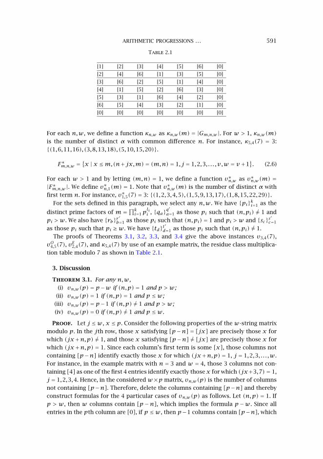
Table 2.1

[1] [2] [3] [4] [5] [6] [0]

[2] [4] [6] [1] [3] [5] [0]

[3] [6] [2] [5] [1] [4] [0]

[4] [1] [5] [2] [6] [3] [0]

[5] [3] [1] [6] [4] [2] [0]

[6] [5] [4] [3] [2] [1] [0]

[0] [0] [0] [0] [0] [0] [0]

For each n,w, we define a function κn,w as κn,w(m) = |Gm,n,w |. For w > 1, κn,w(m)is the number of distinct α with common difference n. For instance, κ5,4(7) = 3:

{(1,6,11,16),(3,8,13,18),(5,10,15,20)}.

F∗m,n,w ={x | x ≤m,(n+jx,m)= (m,n)= 1,j = 1,2,3, . . . ,v,w = v+1

}. (2.6)

For each w > 1 and by letting (m,n) = 1, we define a function υ∗n,w as υ∗n,w(m) =|F∗m,n,w |. We define υ∗n,1(m) = 1. Note that υ∗n,w(m) is the number of distinct α with

first term n. For instance, υ∗1,5(7)= 3: {(1,2,3,4,5),(1,5,9,13,17),(1,8,15,22,29)}.For the sets defined in this paragraph, we select any n,w. We have {pi}ki=1 as the

distinct prime factors of m =∏ki=1p

lii , {qa}q

′a=1 as those pi such that (n,pi) �= 1 and

pi >w. We also have {rb}r ′b=1 as those pi such that (n,pi)= 1 and pi >w and {sc}s′c=1

as those pi such that pi ≥w. We have {td}t′d=1 as those pi such that (n,pi) �= 1.

The proofs of Theorems 3.1, 3.2, 3.3, and 3.4 give the above instances υ3,4(7),υO4,5(7), υ

E2,4(7), and κ5,4(7) by use of an example matrix, the residue class multiplica-

tion table modulo 7 as shown in Table 2.1.

3. Discussion

Theorem 3.1. For any n,w,

(i) υn,w(p)= p−w if (n,p)= 1 and p >w;

(ii) υn,w(p)= 1 if (n,p)= 1 and p ≤w;

(iii) υn,w(p)= p−1 if (n,p) �= 1 and p >w;

(iv) υn,w(p)= 0 if (n,p) �= 1 and p ≤w.

Proof. Let j ≤w, x ≤ p. Consider the following properties of the w-string matrix

modulo p. In the jth row, those x satisfying [p−n]= [jx] are precisely those x for

which (jx+n,p) �= 1, and those x satisfying [p−n] �= [jx] are precisely those x for

which (jx+n,p)= 1. Since each column’s first term is some [x], those columns not

containing [p−n] identify exactly those x for which (jx+n,p)= 1, j = 1,2,3, . . . ,w.

For instance, in the example matrix with n = 3 and w = 4, those 3 columns not con-

taining [4] as one of the first 4 entries identify exactly thosex for which (jx+3,7)= 1,

j = 1,2,3,4. Hence, in the consideredw×p matrix, υn,w(p) is the number of columns

not containing [p−n]. Therefore, delete the columns containing [p−n] and thereby

construct formulas for the 4 particular cases of υn,w(p) as follows. Let (n,p) = 1. If

p > w, then w columns contain [p−n], which implies the formula p−w. Since all

entries in the pth column are [0], if p ≤w, then p−1 columns contain [p−n], which


implies the formula p−(p−1) = 1. Let (n,p) �= 1 (and thus [0] = [p−n]). If p > w,

then 1 column contains [0], which implies the formula p−1. Since all entries in the

pth row are [0], if p ≤w, then all p columns contain [0], which implies the formula

p−p = 0.

Theorem 3.2. For any w with w = 2v+1 let (n,p)= 1. Then

(i) υOn,w(p)= p−w+1 if p ≥w;

(ii) υOn,w(p)= 1 if p <w.

Proof. Let j ≤ v , x ≤ p. Consider the following properties of the v-string matrix

modulo p. In the jth row, those x satisfying [n]= [jx] or [p−n]= [jx] are precisely

those x for which (jx−n,p) �= 1 or (jx+n,p) �= 1, and those x satisfying [n] �= [jx]and [p−n] �= [jx] are precisely those x for which (jx−n,p)= (jx+n,p)= 1. Since

each column’s first term is some [x], those columns not containing [n] or [p−n]identify exactly those x for which (jx−n,p) = (jx+n,p) = 1, j = 1,2,3, . . . ,v . For

instance, in the example matrix with n= 4 andw = 5, those 3 columns not containing

[4] or [3] as one of the first 2 entries identify exactly those x for which (jx−4,7)=(jx+4,7)= 1, j = 1,2. Hence, in the considered v×pmatrix, υOn,w(p) is the number of

columns not containing [n] or [p−n]. Therefore, delete the columns containing [n] or

[p−n] and thereby construct formulas for the 2 particular cases of υOn,w(p) as follows:

if p ≥w, then v columns contain [n], v columns contain [p−n], and no one column

contains both [n] and [p−n] (since in each of the first p−1 columns in the residue

class multiplication table modulo p, the index of one of these entries exceeds v).

Therefore 2v = w − 1 columns contain [n] or [p −n] which implies the formula

p−(w−1)= p−w+1. Since all entries in the pth column are [0], if p <w, then p−1

columns contain [n] or [p−n] which implies the formula p−(p−1)= 1.

Theorem 3.3. For any n,w with w = 2v ,

(i) υEn,w(p)= p−w if (n,p)= 1 and p >w;

(ii) υEn,w(p)= 1 if p = 2 or if p is odd and (n,p)= 1 and p <w;

(iii) υEn,w(p)= p−1 if (n,p) �= 1 and p >w;

(iv) υEn,w(p)= 0 if p is odd and (n,p) �= 1 and p <w.

Proof. Let j ≤ v , x ≤ p. For the w-string matrix modulo p, to consider only

the odd-indexed entries in the columns, we eliminate the even-indexed rows. Con-

sider the following properties of the resulting v×p matrix whose xth column is the

sequence {[(2j − 1)x]}vj=1. In the jth row, those x satisfying [n] = [(2j − 1)x] or

[p−n]= [(2j−1)x] are precisely those x for which ((2j−1)x−n,p) �= 1 or ((2j−1)x+n,p) �= 1, and those x satisfying [n] �= [(2j−1)x] and [p−n] �= [(2j−1)x]are precisely those x for which ((2j−1)x−n,p) = ((2j−1)x+n,p) = 1. Since each

column’s first term is some [x], those columns not containing [n] or [p−n] identify

exactly those x for which ((2j−1)x−n,p) = ((2j−1)x+n,p) = 1, j = 1,2,3, . . . ,v .

For instance, in the example matrix with n = 2 and w = 4, those 3 columns not

containing [2] or [5] as one of the first 2 odd-indexed entries identify exactly those

x for which ((2j−1)x−2,7) = ((2j−1)x+2,7) = 1, j = 1,2. Hence, in the obtained

v×p matrix, υEn,w(p) is the number of columns not containing [n] or [p−n]. There-

fore, we delete the columns containing [n] or [p−n] and thereby construct formulas


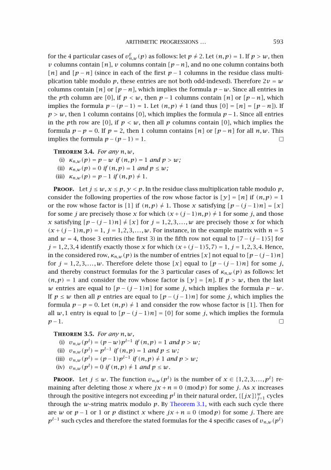
for the 4 particular cases of υEn,w(p) as follows: let p �= 2. Let (n,p)= 1. If p >w, then

v columns contain [n], v columns contain [p−n], and no one column contains both

[n] and [p−n] (since in each of the first p−1 columns in the residue class multi-

plication table modulo p, these entries are not both odd-indexed). Therefore 2v =wcolumns contain [n] or [p−n], which implies the formula p−w. Since all entries in

the pth column are [0], if p < w, then p−1 columns contain [n] or [p−n], which

implies the formula p− (p−1) = 1. Let (n,p) �= 1 (and thus [0] = [n] = [p−n]). If

p >w, then 1 column contains [0], which implies the formula p−1. Since all entries

in the pth row are [0], if p < w, then all p columns contain [0], which implies the

formula p−p = 0. If p = 2, then 1 column contains [n] or [p−n] for all n,w. This

implies the formula p−(p−1)= 1.


(i) κn,w(p)= p−w if (n,p)= 1 and p >w;

(ii) κn,w(p)= 0 if (n,p)= 1 and p ≤w;

(iii) κn,w(p)= p−1 if (n,p) �= 1.

Proof. Let j ≤w, x ≤ p, y <p. In the residue class multiplication table modulo p,

consider the following properties of the row whose factor is [y] = [n] if (n,p) = 1

or the row whose factor is [1] if (n,p) �= 1. Those x satisfying [p− (j−1)n] = [x]for some j are precisely those x for which (x+(j−1)n,p) �= 1 for some j, and those

x satisfying [p− (j−1)n] �= [x] for j = 1,2,3, . . . ,w are precisely those x for which

(x+(j−1)n,p) = 1, j = 1,2,3, . . . ,w. For instance, in the example matrix with n = 5

and w = 4, those 3 entries (the first 3) in the fifth row not equal to [7−(j−1)5] for

j = 1,2,3,4 identify exactly those x for which (x+(j−1)5,7)= 1, j = 1,2,3,4. Hence,

in the considered row, κn,w(p) is the number of entries [x] not equal to [p−(j−1)n]for j = 1,2,3, . . . ,w. Therefore delete those [x] equal to [p− (j−1)n] for some j,and thereby construct formulas for the 3 particular cases of κn,w(p) as follows: let

(n,p) = 1 and consider the row whose factor is [y] = [n]. If p > w, then the last

w entries are equal to [p− (j−1)n] for some j, which implies the formula p−w.

If p ≤w then all p entries are equal to [p− (j−1)n] for some j, which implies the

formula p−p = 0. Let (n,p) �= 1 and consider the row whose factor is [1]. Then for

all w,1 entry is equal to [p− (j−1)n] = [0] for some j, which implies the formula

p−1.


(i) υn,w(pl)= (p−w)pl−1 if (n,p)= 1 and p >w;

(ii) υn,w(pl)= pl−1 if (n,p)= 1 and p ≤w;

(iii) υn,w(pl)= (p−1)pl−1 if (n,p) �= 1 and p >w;

(iv) υn,w(pl)= 0 if (n,p) �= 1 and p ≤w.

Proof. Let j ≤ w. The function υn,w(pl) is the number of x ∈ {1,2,3, . . . ,pl} re-

maining after deleting those x where jx+n ≡ 0 (modp) for some j. As x increases

through the positive integers not exceeding pl in their natural order, {[jx]}wj=1 cycles

through the w-string matrix modulo p. By Theorem 3.1, with each such cycle there

are w or p−1 or 1 or p distinct x where jx+n ≡ 0 (modp) for some j. There are

pl−1 such cycles and therefore the stated formulas for the 4 specific cases of υn,w(pl)


are immediate:

(i) pl−wpl−1 = (p−w)pl−1;

(ii) pl−(p−1)pl−1 = pl−1;

(iii) pl−pl−1 = (p−1)pl−1;

(iv) pl−ppl−1 = 0.

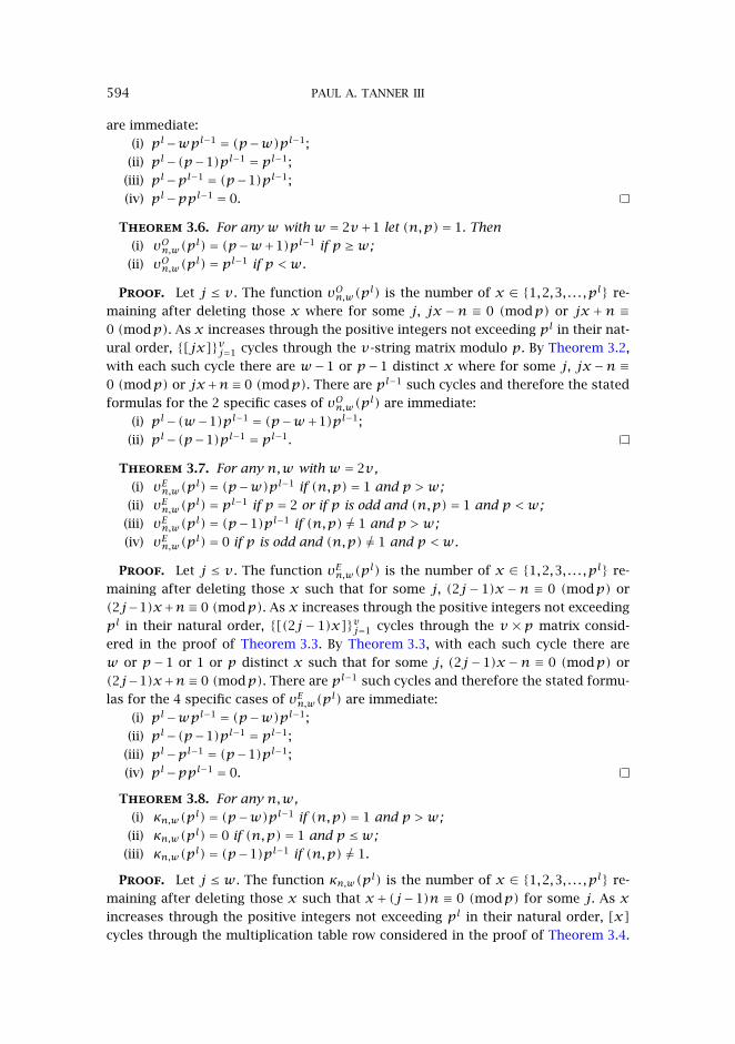
Theorem 3.6. For any w with w = 2v+1 let (n,p)= 1. Then

(i) υOn,w(pl)= (p−w+1)pl−1 if p ≥w;

(ii) υOn,w(pl)= pl−1 if p <w.

Proof. Let j ≤ v . The function υOn,w(pl) is the number of x ∈ {1,2,3, . . . ,pl} re-

maining after deleting those x where for some j, jx−n ≡ 0 (modp) or jx+n ≡0 (modp). As x increases through the positive integers not exceeding pl in their nat-

ural order, {[jx]}vj=1 cycles through the v-string matrix modulo p. By Theorem 3.2,

with each such cycle there are w−1 or p−1 distinct x where for some j, jx−n ≡0 (modp) or jx+n≡ 0 (modp). There are pl−1 such cycles and therefore the stated

formulas for the 2 specific cases of υOn,w(pl) are immediate:

(i) pl−(w−1)pl−1 = (p−w+1)pl−1;

(ii) pl−(p−1)pl−1 = pl−1.

Theorem 3.7. For any n,w with w = 2v ,

(i) υEn,w(pl)= (p−w)pl−1 if (n,p)= 1 and p >w;

(ii) υEn,w(pl)= pl−1 if p = 2 or if p is odd and (n,p)= 1 and p <w;

(iii) υEn,w(pl)= (p−1)pl−1 if (n,p) �= 1 and p >w;

(iv) υEn,w(pl)= 0 if p is odd and (n,p) �= 1 and p <w.

Proof. Let j ≤ v . The function υEn,w(pl) is the number of x ∈ {1,2,3, . . . ,pl} re-

maining after deleting those x such that for some j, (2j−1)x−n ≡ 0 (modp) or

(2j−1)x+n≡ 0 (modp). As x increases through the positive integers not exceeding

pl in their natural order, {[(2j − 1)x]}vj=1 cycles through the v ×p matrix consid-

ered in the proof of Theorem 3.3. By Theorem 3.3, with each such cycle there are

w or p−1 or 1 or p distinct x such that for some j, (2j−1)x−n ≡ 0 (modp) or

(2j−1)x+n≡ 0 (modp). There are pl−1 such cycles and therefore the stated formu-

las for the 4 specific cases of υEn,w(pl) are immediate:


(ii) pl−(p−1)pl−1 = pl−1;

(iii) pl−pl−1 = (p−1)pl−1;

(iv) pl−ppl−1 = 0.


(i) κn,w(pl)= (p−w)pl−1 if (n,p)= 1 and p >w;

(ii) κn,w(pl)= 0 if (n,p)= 1 and p ≤w;

(iii) κn,w(pl)= (p−1)pl−1 if (n,p) �= 1.

Proof. Let j ≤ w. The function κn,w(pl) is the number of x ∈ {1,2,3, . . . ,pl} re-

maining after deleting those x such that x+ (j−1)n ≡ 0 (modp) for some j. As xincreases through the positive integers not exceeding pl in their natural order, [x]cycles through the multiplication table row considered in the proof of Theorem 3.4.


By Theorem 3.4, with each such cycle there are w or p or 1 distinct x such that

x+(j−1)n≡ 0 (modp) for some j. There are pl−1 such cycles; therefore, the stated

formulas for the 3 specific cases of κn,w(pl) are immediate:


(ii) pl−ppl−1 = 0;

(iii) pl−pl−1 = (p−1)pl−1.

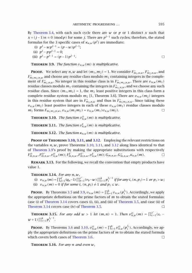
Theorem 3.9. The function υn,w(m) is multiplicative.

Proof. We select any n,w and let (m1,m2)= 1. We consider F+m1,n,w , F+m2,n,w , and

F+m1m2,n,w and choose any residue class modulom1 containing integers in the comple-

ment of F+m1,n,w . No integer in this residue class is in F+m1m2,n,w . There are υn,w(m1)residue classes modulom1 containing the integers in F+m1,n,w , and we choose any such

residue class. Since (m1,m2) = 1, the m2 least positive integers in this class form a

complete residue system modulo m2 [1, Theorem 3.6]. There are υn,w(m2) integers

in this residue system that are in F+m2,n,w and thus in F+m1m2,n,w . Since taking these

υn,w(m2) least positive integers in each of these υn,w(m1) residue classes modulo

m1 forms Fm1m2,n,w , υn,w(m1m2)= υn,w(m1)υn,w(m2).

Theorem 3.10. The function υOn,w(m) is multiplicative.

Theorem 3.11. The function υEn,w(m) is multiplicative.

Theorem 3.12. The function κn,w(m) is multiplicative.

Proof of Theorems 3.10, 3.11, and 3.12. Employing the relevant restrictions on

the variables n,w, prove Theorems 3.10, 3.11, and 3.12 along lines identical to that

of Theorem 3.9’s proof by making the appropriate substitutions with respectively

FOm,n,w,FO+

m,n,w,υOn,w(m); FEm,n,w,FE+

m,n,w,υEn,w(m); Gm,n,w,G+m,n,w,κn,w(m).

Remark 3.13. For the following, we recall the convention that empty products have

value 1.


(i) υn,w(m)=∏q′a=1(qa−1)

∏r ′b=1(rb−w)

∏ki=1p

li−1i if for any i, (n,pi)=1 or pi>w;

(ii) υn,w(m)= 0 if for some i, (n,pi) �= 1 and pi ≤w.

Proof. By Theorems 3.5 and 3.9, υn,w(m)=∏ki=1υn,w(p

lii ). Accordingly, we apply

the appropriate definitions on the prime factors of m to obtain the stated formulas:

case (i) of Theorem 3.14 covers cases (i), (ii), and (iii) of Theorem 3.5, and case (ii) of

Theorem 3.14 covers case (iv) of Theorem 3.5.

Theorem 3.15. For any odd w > 1 let (m,n) = 1. Then υOn,w(m) =∏s′c=1(sc −

w+1)∏ki=1p

li−1i .

Proof. By Theorems 3.6 and 3.10, υOn,w(m)=∏ki=1υOn,w(p

lii ). Accordingly, we ap-

ply the appropriate definitions on the prime factors ofm to obtain the stated formula

which covers both cases of Theorem 3.6.

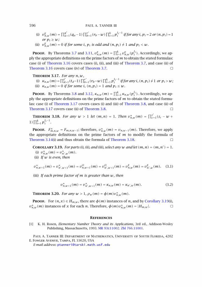
Theorem 3.16. For any n and even w,


(i) υEn,w(m)=∏q′a=1(qa−1)

∏r ′b=1(rb−w)

∏ki=1p

li−1i if for any i,pi=2 or (n,pi)=1

or pi ≥w;

(ii) υEn,w(m)= 0 if for some i, pi is odd and (n,pi) �= 1 and pi <w.

Proof. By Theorems 3.7 and 3.11, υEn,w(m)=∏ki=1υEn,w(p


ply the appropriate definitions on the prime factors ofm to obtain the stated formulas:

case (i) of Theorem 3.16 covers cases (i), (ii), and (iii) of Theorem 3.7, and case (ii) of

Theorem 3.16 covers case (iv) of Theorem 3.7.


(i) κn,w(m)=∏t′d=1(td−1)

∏r ′b=1(rb−w)

∏ki=1p

li−1i if for any i, (n,pi) �=1 or pi>w;

(ii) κn,w(m)= 0 if for some i, (n,pi)= 1 and pi ≤w.

Proof. By Theorems 3.8 and 3.12, κn,w(m)=∏ki=1κn,w(p


ply the appropriate definitions on the prime factors of m to obtain the stated formu-

las: case (i) of Theorem 3.17 covers cases (i) and (iii) of Theorem 3.8, and case (ii) of

Theorem 3.17 covers case (ii) of Theorem 3.8.

Theorem 3.18. For any w > 1 let (m,n) = 1. Then υ∗n,w(m) =∏s′c=1(sc −w +

1)∏ki=1p

li−1i .

Proof. F∗m,n,w = Fm,n,w−1; therefore, υ∗n,w(m) = υn,w−1(m). Therefore, we apply

the appropriate definitions on the prime factors of m to modify the formula of

Theorem 3.14(i) and thus obtain the formula of Theorem 3.18.

Corollary 3.19. For parts (i), (ii), and (iii), select anyw and let (m,n)= (m,n′)= 1.

(i) υ∗n,w(m)= υ∗n′,w(m).(ii) If w is even, then

υ∗n,w+1(m)= υ∗n′,w+1(m)= υOn,w+1(m)= υOn′,w+1(m)= υEn,w(m)= υEn′,w(m). (3.1)

(iii) If each prime factor of m is greater than w, then

υ∗n,w+1(m)= υ∗n′,w+1(m)= κn,w(m)= κn′,w(m). (3.2)

Theorem 3.20. For any w > 1, ρw(m)=φ(m)υ∗n,w(m).

Proof. For (n,x)∈Hm,w , there areφ(m) instances of n, and by Corollary 3.19(i),

υ∗n,w(m) instances of x for each n. Therefore, φ(m)υ∗n,w(m)= |Hm,w |.

References

[1] K. H. Rosen, Elementary Number Theory and its Applications, 3rd ed., Addison-WesleyPublishing, Massachusetts, 1993. MR 93i:11002. Zbl 766.11001.

Paul A. Tanner III: Department of Mathematics, University of South Florida, 4202E. Fowler Avenue, Tampa, FL 33620, USA

E-mail address: [email protected]

http://www.ams.org/mathscinet-getitem?mr=93i:11002

http://www.emis.de/cgi-bin/MATH-item?766.11001

mailto:[email protected]

Submit your manuscripts athttp://www.hindawi.com

Hindawi Publishing Corporationhttp://www.hindawi.com Volume 2014

MathematicsJournal of


Mathematical Problems in Engineering

Hindawi Publishing Corporationhttp://www.hindawi.com

Differential EquationsInternational Journal of

Volume 2014

Applied MathematicsJournal of


Probability and StatisticsHindawi Publishing Corporationhttp://www.hindawi.com Volume 2014

Journal of


Mathematical PhysicsAdvances in

Complex AnalysisJournal of


OptimizationJournal of


CombinatoricsHindawi Publishing Corporationhttp://www.hindawi.com Volume 2014

International Journal of


Operations ResearchAdvances in

Journal of


Function Spaces

Abstract and Applied AnalysisHindawi Publishing Corporationhttp://www.hindawi.com Volume 2014

International Journal of Mathematics and Mathematical Sciences


The Scientific World JournalHindawi Publishing Corporation http://www.hindawi.com Volume 2014


Algebra

Discrete Dynamics in Nature and Society



Decision SciencesAdvances in

Discrete MathematicsJournal of

Hindawi Publishing Corporationhttp://www.hindawi.com

Volume 2014 Hindawi Publishing Corporationhttp://www.hindawi.com Volume 2014

Stochastic AnalysisInternational Journal of

Documents

Arithmetic progressions that consist only of reduced residues