DEPARTMENT OF ECONOMICS AND SOCIETY, DALARNA UNIVERSITY ONE-YEAR MASTER THESIS IN STATISTICS 2008

  

Applying ARIMA Model to the Analysis of Monthly 

Temperature of Stockholm    

Authors: Junquan Xiang

Supervisor: Mikael Möller

Submitted on: June 22, 2008

AbstractThe temperature measurement which is always important for studying climate change

has received much more attention in recent years. The main aim of this paper is to

find an appropriate model for a given daily average temperature series that is from

1756 to 2007 in Stockholm. Data used in this paper has been adjusted by Anders

Moberg and his colleagues. Based on the features of data, we consider the class of

ARIMA (autoregressive integrated moving average) models. Finally, we find a

seasonal ARIMA (SARIMA) model to fit the data. It indicates that there exists a

stable structure in this temperature series. It can also be verified by fitting ARIMA

models to each subseries for 25 years periods. On the other hand, a graphical method

is applied to analyze the temperature series in order to detect outliers. The results

reveal even the strongest outlier has weak effect on the stable temperature structure.

Key words: Box-Jenkins methodology, ARIMA model, SARIMA model, outlier.

Table of Contents 

1 Introduction ............................................................................................................1 2 Models and Statistical methodology.......................................................................2

2.1 Autoregressive integrated moving average （ARIMA）models ..................2 2.2 Multiplicative Seasonal ARIMA Models ........................................................3 2.3 The Box-Jenkins (BJ) methodology................................................................3

3 Data description......................................................................................................4 3.1 Data sources ....................................................................................................4 3.2 Data transformation.........................................................................................5

4 Model building .......................................................................................................7 4.1 Identification ...................................................................................................7 4.2 Estimation........................................................................................................8 4.3 Diagnostic checking ........................................................................................9

5 Outliers detection..................................................................................................11 6 Conclusion............................................................................................................13 References....................................................................................................................14 Appendix I : Tables ......................................................................................................15 Appendix II : R codes ..................................................................................................16

1 Introduction

In recent years, more and more people focus on the climate change of the Earth. This is the

greatest and most important environmental challenge of our time. A lot of scholars prefer to

use the average temperature measurement to study the climatic changes in Sweden. In this

paper, we will study the long range of daily temperature data from Stockholm, 252 years

ranging from 1756 to 2007. The data has been transformed to degree Celsius by Anders

Moberg1 and his colleagues. This was necessary because many different thermometers were

used. These daily data also has been reconstructed and homogenized back to 1756. Due to the

good quality of the daily data, we are able to use them directly to look for the structure in this

temperature series.

There are two purposes for this paper: Initially we will introduce the ACF (the

autocorrelation function) and PACF (the partial autocorrelation function) as tools to fit a

univariate ARIMA (autoregressive integrated moving average) model to the data. We will

then use these tools to find ARIMA models for different parts of the series to unveil hidden

stable structures in the temperature series. In this procedure we will look at periods of 25

years to check whether those 10 series (25*10=250) have the same structure as the whole

series. Secondly we will look for outliers in the series. If they exist we also wonder how the

outliers affect the structure of the whole series.

The remainder of this thesis is organized as follows:

In Chapter 2, we introduce the model and statistical methodology used in this paper. In

Chapter 3, we give a brief data description and data transformation. Chapter 4 provides the

procedure of model building, estimation and combines some data analysis of the temperature

subseries. In Chapter 5, we show the outliers detection procedure. Lastly chapter 6 presents

the results and provides my conclusions.

1 Department of Physical Geography and Quaternary Geology, Stockholm University, SE-106 91 Stockholm.

1

2 Models and Statistical methodology

Because of the look of the original data (see Figure 1) we consider fitting ARIMA models to

the data. Here, we introduce the model and the statistical methodology which will be used in

this paper.

2.1 Autoregressive integrated moving average （ARIMA）

models

In statistics, an autoregressive integrated moving average (ARIMA) model is a generalization

of an autoregressive moving average or (ARMA) model. These models are fitted to time

series data either to better understand the data or to predict future points in the series. The

model is generally referred to as an ARIMA ( , d , ) model where , , and are

integers greater than or equal to zero. The first parameter ( ) refers to the number of

autoregressive lags (not counting the unit roots), the second parameter ( ) refers to the order

of integration, and the third parameter ( ) gives the number of moving average lags.

p q p d q

p

d

q

2

xA process, is said to be ARIMA ( , , ) if is ARMA( , ). In

general, we will write the model as

{ }tx p d q ( )1 ddt tx B∇ = − p q

( )( ) ( )1 dt tB B x B wφ θ− = { } (, )20,tw WN σ∼

k

Bφ

Bθ

.

Here, we define the backshift operator by and the autoregressive operator and

moving average operator are defined as follows:

kt tB x x −=

( ) 21 21 p

pB B Bφ φ φ= − − − −

( ) 21 21 q

qB B Bθ θ θ= + + + + .

( ) 0Bφ ≠ for 1B ≤ , the process is stationary if and only if , in which case

it reduces to an ARMA

{ }tx 0d =

( ),p q process.

2.2 Multiplicative Seasonal ARIMA Models

3

st

This model is a modification to the ARIMA model because of seasonal and nonstationary

behavior. In this paper the data figures will show a strong yearly seasonal component at

seasonal level 12. The pure seasonal ARMA model, ARMA , take the

form , the seasonal autoregressive operator and the seasonal moving

average operator of orders P and Q with seasonal period s are given respectively as

follows:

( , )sP Q

( ) ( )sP t QB x B wΦ = Θ

( ) 21 21s s s

P PB B BΦ = −Φ −Φ − −Φ PsB

QsB

( ) 21 21s s s

Q QB B BΘ = +Θ +Θ + +Θ .

In general, we can combine the seasonal and nonseasonal operators into a multiplicative

seasonal autoregressive moving average model, denoted by ARMA( ), ( , sp q P Q× )

t

, and write

( ) ( ) ( ) ( )s sP t QB B x B B wφ θΦ = Θ

as the overall model.

The multiplicative seasonal autoregressive integrated moving average model, or SARIMA

model, of Box and Jenkins (1970) is given by

( ) ( ) ( ) ( )s D d sP s t QB B x B Bφ α θΦ ∇ ∇ = +Θ tw

where is the causal Gaussian white noise process. The general model is denoted as

ARIMA( ) . The ordinary autoregressive and moving average components

are represented by polynomials and

tw

, , ( , , )sp d q P D Q×

( )Bφ ( )Bθ of orders and q , respectively (see

above), and the seasonal autoregressive and moving average components by polynomials

and (see above) of orders P and Q and ordinary and seasonal difference

components by and

p

( sP BΦ ) )

)

( sQ BΘ

(1 dd B∇ = − ( )1 DD ss B∇ = − .

2.3 The Box-Jenkins (BJ) methodology

Given a time series, how can we know whether it follows an ARIMA process or not. The

Box-Jenkins (BJ) methodology is one answer to the above question. The BJ methodology is

an iterative process, which is named after the statisticians George Box and Gwilym Jenkins.

It applies autoregressive moving average ARMA or ARIMA models to find the best fit of a

time series to past values of this time series, in order to make forecasts.

Generally, the BJ method consists of four steps: Identification; Estimation; Diagnostic

checking and Forecasting[4]. The procedure relies heavily on plots of the ACF and the PACF

to find out the appropriate values of , and q . When values of , and q have

been found, we estimate the parameters in the model. In the third step, we check whether the

chosen model fits the data well. Here we check if the residuals of the identified model are

white noise or not. If so, we accept the model; if not, we have to find another improved

model. Lastly we use the model for forecasting, but we don’t emphasis on forecasting future

values in this paper.

p d p d

3 Data description

3.1 Data sources

The available historical data are taken from Anders Moberg. They consist of the daily

average temperatures from 1756 to 2007 in Stockholm. This long series is reconstructed by

Anders Moberg and his colleagues. They compiled it to be able to study the climate change

during this period.

There are three kinds of data in the records. The first kind is the raw data of the daily average

temperature according to observations. The second set of data is the daily average

temperature after homogenization and with gaps filled in using data from Uppsala. The third

set of data is the second adjusted for a supposed warm bias of MJJA (May, June, July and

August) temperature before September of 1858. Because there are different thermometers

used in the temperature records, it is necessary to adjust the data to obtain the series with

good quality.

Considering the adjustment of data, we will use the third set of data to analyze the

temperature structure in Stockholm. These data can represent the real temperature values

with smaller errors.

4

3.2 Data transformation

The long temperature records consisted of the average temperature during each day of the

previous 252 years, starting on the first day of January. The number of records was too large

to deal with easily. We therefore transformed the daily average temperatures to monthly

average temperatures. Monthly data will also represent the “true” average temperature in a

better way. The data were reduced to monthly averages by dividing each monthly total by the

number of days in the month. There are 3024 months measured from the first month of 1756

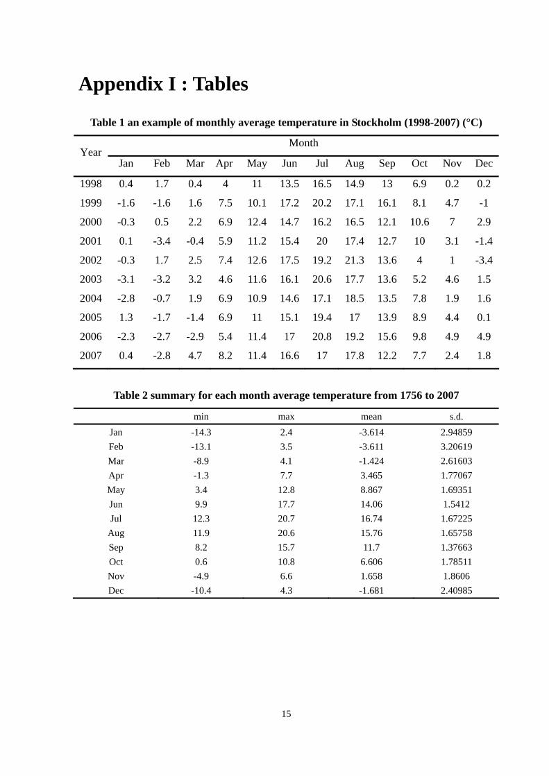
to the last month of 2007. The table of the transformed temperature series sample is given in

the Appendix I. Secondly, before using the BJ methodology, we should note that the time

series must be stationary or may become stationary after one or more differencings[4]. We

must ensure that the time series being analyzed is stationary before we are able to specify a

model.

monthly temperature(1756-2007)

Time

cent

igra

de

0 500 1500 2500

-15

-55

15

differenced temperature series

Time

z

0 500 1500 2500

-10

05

10

monthly temperature(1983-2007)

Time

cent

ideg

ree

0 50 150 250

-10

05

15

differenced temperature series

Time

cent

igra

de

0 50 150 250

-10

-50

510

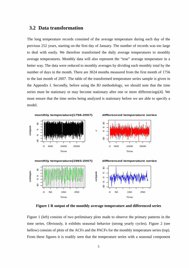
Figure 1 R output of the monthly average temperature and differenced series

Figure 1 (left) consists of two preliminary plots made to observe the primary patterns in the

time series. Obviously, it exhibits seasonal behavior (strong yearly cycles). Figure 2 (see

bellow) consists of plots of the ACFs and the PACFs for the monthly temperature series (top).

From these figures it is readily seen that the temperature series with a seasonal component

5

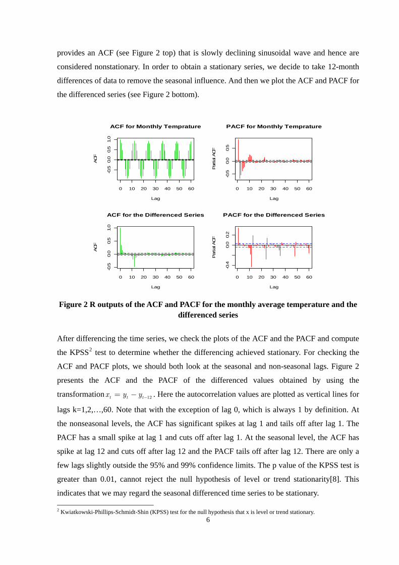
provides an ACF (see Figure 2 top) that is slowly declining sinusoidal wave and hence are

considered nonstationary. In order to obtain a stationary series, we decide to take 12-month

differences of data to remove the seasonal influence. And then we plot the ACF and PACF for

the differenced series (see Figure 2 bottom).

0 10 20 30 40 50 60

-0.5

0.0

0.5

1.0

Lag

ACF

ACF for Monthly Temprature

0 10 20 30 40 50 60

-0.5

0.0

0.5

Lag

Par

tial A

CF

PACF for Monthly Temprature

0 10 20 30 40 50 60

-0.5

0.0

0.5

1.0

Lag

ACF

ACF for the Differenced Series

0 10 20 30 40 50 60

-0.4

0.0

0.2

Lag

Par

tial A

CF

PACF for the Differenced Series

Figure 2 R outputs of the ACF and PACF for the monthly average temperature and the

differenced series

After differencing the time series, we check the plots of the ACF and the PACF and compute

the KPSS2 test to determine whether the differencing achieved stationary. For checking the

ACF and PACF plots, we should both look at the seasonal and non-seasonal lags. Figure 2

presents the ACF and the PACF of the differenced values obtained by using the

transformation . Here the autocorrelation values are plotted as vertical lines for

lags k=1,2,…,60. Note that with the exception of lag 0, which is always 1 by definition. At

the nonseasonal levels, the ACF has significant spikes at lag 1 and tails off after lag 1. The

PACF has a small spike at lag 1 and cuts off after lag 1. At the seasonal level, the ACF has

spike at lag 12 and cuts off after lag 12 and the PACF tails off after lag 12. There are only a

few lags slightly outside the 95% and 99% confidence limits. The p value of the KPSS test is

greater than 0.01, cannot reject the null hypothesis of level or trend stationarity

12t t tx y y −= −

[8]. This

indicates that we may regard the seasonal differenced time series to be stationary.

62 Kwiatkowski-Phillips-Schmidt-Shin (KPSS) test for the null hypothesis that x is level or trend stationary.

4 Model building

4.1 Identification

After suitably transforming the data, the next step is to identify preliminary values of the

autoregressive order , the order of differencing , and the moving average order . We

utilize again the ACF and the PACF plots to determine the order of an ARIMA model. Here,

observing the series which has no drift, we can write the model without drift parameter.

p d q

According to spikes shown in the Figure 2, the PACF has spikes at lag 1 and cuts off after lag

1 at the nonseasonal level and the ACF are tailing off. Using Table 1, it suggests a

nonseasonal autoregressive of order =1. We use to denote the differenced monthly

temperature series and represent the original monthly temperature series. Therefore, we

tentatively identify the following nonseasonal autoregressive model

p tx

ty

7

tw1 1t tx xφ −= +

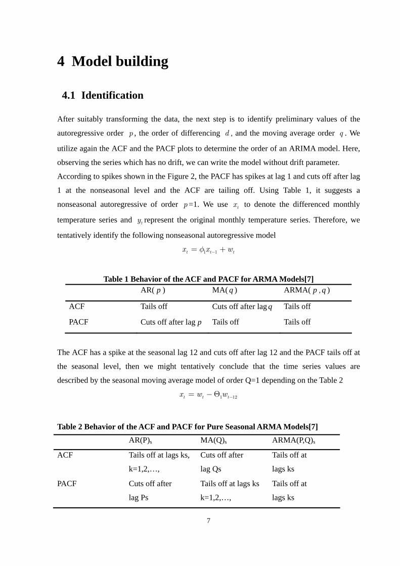
Table 1 Behavior of the ACF and PACF for ARMA Models[7] AR( ) p MA( ) q ARMA( , ) p q

ACF Tails off Cuts off after lag q Tails off

PACF Cuts off after lag p Tails off Tails off

The ACF has a spike at the seasonal lag 12 and cuts off after lag 12 and the PACF tails off at

the seasonal level, then we might tentatively conclude that the time series values are

described by the seasonal moving average model of order Q=1 depending on the Table 2

1 1t t tx w w −= −Θ 2

Table 2 Behavior of the ACF and PACF for Pure Seasonal ARMA Models[7]

AR(P)s MA(Q)s ARMA(P,Q)s

ACF Tails off at lags ks,

k=1,2,…,

Cuts off after

lag Qs

Tails off at

lags ks

PACF Cuts off after

lag Ps

Tails off at lags ks

k=1,2,…,

Tails off at

lags ks

Combing these two models, we obtain the overall model

8

21 1 1 1t t t tx x w wφ − −= + −Θ

Actually, this is a mixed seasonal model which I mentioned in the methodology part. It

combines the nonseasonal and seasonal operator into the multiplicative seasonal ARIMA

model. Since taking th differences of an ARIMA (d p , , ) produces a stationary

ARMA( , ) process. We exhibit the equations for the model, denoted by

ARIMA

d q

p q

( )p,d,q × s(P,D,Q) , in the notation given above, where the seasonal fluctuations

occur every 12 months. Then we fit the ARIMA( ) to the differenced monthly

temperature data, the process can be written as follows:

121, 0, 0 (0,1,1)×

( ) ( )d st QB x B wφ ∇ = Θ t

( )( ) ( )0 121 11 1 1t tB B x Bφ− − = +Θ w

2ty

12

2−

2

Because taking 12th differences, the original series can be written as

form , ( )1 112 1t tx y B= ∇ = −

( )( )1 12 11 t t t tB y y w wφ − −− − = +Θ

12 1 1 1 13 1 1t t t t t ty y y y w wφ φ− − −− − + = +Θ

After determining the values of and , we should check if the values are

appropriate. Plot the ACF and the PACF of the chosen model firstly. Then comparing with

the TACF (theoretical autocorrelation function) and the TPACF (theoretical partial

autocorrelation function) plots where the orders are known, we can find that those plots have

the similar pattern of the spikes.

p,d,q P,D,Q

Therefore, we can obtain the final model as follows:

1 1 12 1 13 1 1t t t t t ty y y y w wφ φ− − − −= + − + +Θ

4.2 Estimation

For the ARIMA (1,0,0)×(0,1,1)12 model obtained above we estimate the parameters with the

statistical software R.

The maximum likelihood estimates of and obtained from R are as follows: 1φ 1Θ

1φ =0.3655 and = -0.9753 1Θ

And then the estimated model is

9

12tw 1 12 130.3655 0.3655 0.9753t t t t ty y y y w− − − −= + − + −

s.e. = (0.0170) (0.0170) (0.0050)

All of the coefficients are significant.

4.3 Diagnostic checking

If the model fits well, the standardized residuals estimated from this model should behave as

an iid (independent and identically distributed) sequence with mean zero and variance .

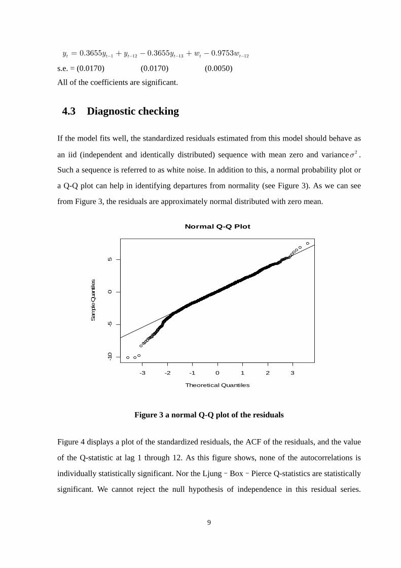
Such a sequence is referred to as white noise. In addition to this, a normal probability plot or

a Q-Q plot can help in identifying departures from normality (see Figure 3). As we can see

from Figure 3, the residuals are approximately normal distributed with zero mean.

2σ

-3 -2 -1 0 1 2 3

-10

-50

5

Normal Q-Q Plot

Theoretical Quantiles

Sam

ple

Qua

ntile

s

Figure 3 a normal Q-Q plot of the residuals

Figure 4 displays a plot of the standardized residuals, the ACF of the residuals, and the value

of the Q-statistic at lag 1 through 12. As this figure shows, none of the autocorrelations is

individually statistically significant. Nor the Ljung–Box–Pierce Q-statistics are statistically

significant. We cannot reject the null hypothesis of independence in this residual series.

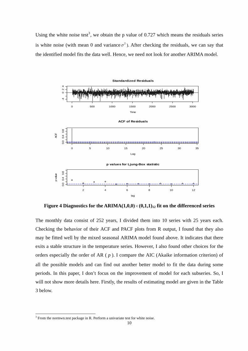
Using the white noise test3, we obtain the p value of 0.727 which means the residuals series

is white noise (with mean 0 and variance ). After checking the residuals, we can say that

the identified model fits the data well. Hence, we need not look for another ARIMA model.

2σ

Standardized Residuals

Time

0 500 1000 1500 2000 2500 3000

-40

24

0 5 10 15 20 25 30 35

0.0

0.4

0.8

Lag

ACF

ACF of Residuals

2 4 6 8 10 12

0.0

0.4

0.8

p values for Ljung-Box statistic

lag

p va

lue

Figure 4 Diagnostics for the ARIMA(1,0,0)×(0,1,1)12 fit on the differenced series

The monthly data consist of 252 years, I divided them into 10 series with 25 years each.

Checking the behavior of their ACF and PACF plots from R output, I found that they also

may be fitted well by the mixed seasonal ARIMA model found above. It indicates that there

exits a stable structure in the temperature series. However, I also found other choices for the

orders especially the order of AR ( ). I compare the AIC (Akaike information criterion) of

all the possible models and can find out another better model to fit the data during some

periods. In this paper, I don’t focus on the improvement of model for each subseries. So, I

will not show more details here. Firstly, the results of estimating model are given in the Table

3 below.

p

103 From the normwn.test package in R. Perform a univariate test for white noise.

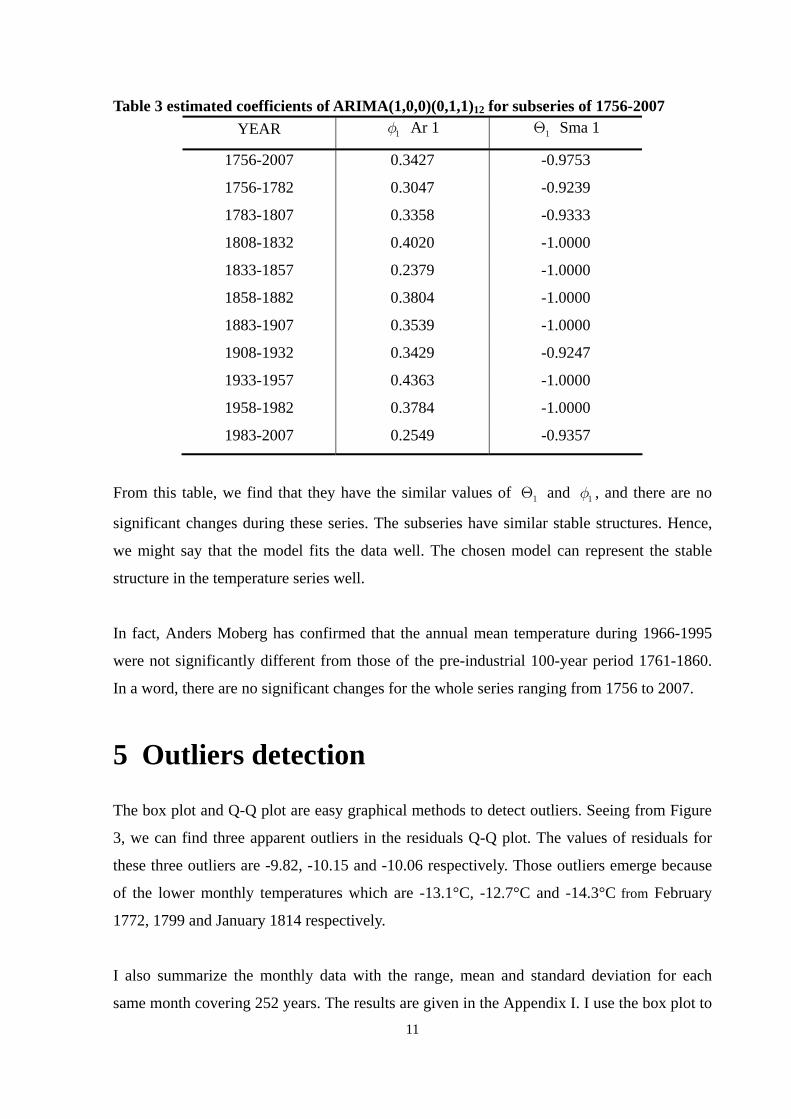
Table 3 estimated coefficients of ARIMA(1,0,0)(0,1,1)12 for subseries of 1756-2007 YEAR 1φ Ar 1 1Θ Sma 1

1756-2007 0.3427 -0.9753

1756-1782 0.3047 -0.9239

1783-1807 0.3358 -0.9333

1808-1832 0.4020 -1.0000

1833-1857 0.2379 -1.0000

1858-1882 0.3804 -1.0000

1883-1907 0.3539 -1.0000

1908-1932 0.3429 -0.9247

1933-1957 0.4363 -1.0000

1958-1982 0.3784 -1.0000

1983-2007 0.2549 -0.9357

From this table, we find that they have the similar values of and , and there are no

significant changes during these series. The subseries have similar stable structures. Hence,

we might say that the model fits the data well. The chosen model can represent the stable

structure in the temperature series well.

1Θ 1φ

In fact, Anders Moberg has confirmed that the annual mean temperature during 1966-1995

were not significantly different from those of the pre-industrial 100-year period 1761-1860.

In a word, there are no significant changes for the whole series ranging from 1756 to 2007.

5 Outliers detection

The box plot and Q-Q plot are easy graphical methods to detect outliers. Seeing from Figure

3, we can find three apparent outliers in the residuals Q-Q plot. The values of residuals for

these three outliers are -9.82, -10.15 and -10.06 respectively. Those outliers emerge because

of the lower monthly temperatures which are -13.1°C, -12.7°C and -14.3°C from February

1772, 1799 and January 1814 respectively.

I also summarize the monthly data with the range, mean and standard deviation for each

same month covering 252 years. The results are given in the Appendix I. I use the box plot to

11

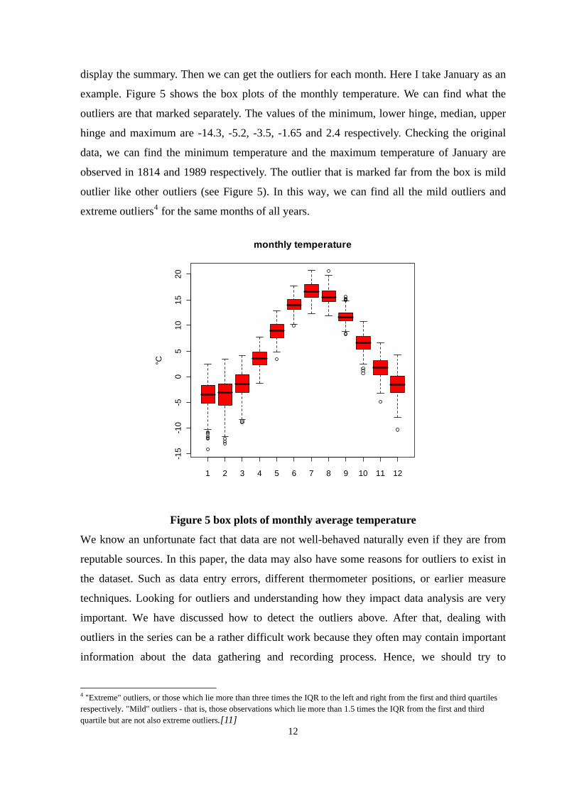
display the summary. Then we can get the outliers for each month. Here I take January as an

example. Figure 5 shows the box plots of the monthly temperature. We can find what the

outliers are that marked separately. The values of the minimum, lower hinge, median, upper

hinge and maximum are -14.3, -5.2, -3.5, -1.65 and 2.4 respectively. Checking the original

data, we can find the minimum temperature and the maximum temperature of January are

observed in 1814 and 1989 respectively. The outlier that is marked far from the box is mild

outlier like other outliers (see Figure 5). In this way, we can find all the mild outliers and

extreme outliers4 for the same months of all years.

1 2 3 4 5 6 7 8 9 10 11 12

-15

-10

-50

510

1520

monthly temperature

°C

Figure 5 box plots of monthly average temperature

We know an unfortunate fact that data are not well-behaved naturally even if they are from

reputable sources. In this paper, the data may also have some reasons for outliers to exist in

the dataset. Such as data entry errors, different thermometer positions, or earlier measure

techniques. Looking for outliers and understanding how they impact data analysis are very

important. We have discussed how to detect the outliers above. After that, dealing with

outliers in the series can be a rather difficult work because they often may contain important

information about the data gathering and recording process. Hence, we should try to

12

4 "Extreme" outliers, or those which lie more than three times the IQR to the left and right from the first and third quartiles respectively. "Mild" outliers - that is, those observations which lie more than 1.5 times the IQR from the first and third quartile but are not also extreme outliers.[11]

13

understand why they exist and whether they will continue to appear before considering the

elimination of these unusual values from the data [12].

Finally, I find out 26 outliers for monthly series using box plots but cannot find the

significant outliers based on the look of box plot of the whole series. We might say those

“outliers” found above have no very strong effects on the stable structure of the whole series.

We can ignore them when we look for the structure in the average temperature series.

6 Conclusion

From the final model found above we see that there is a short term memory of one month and

a long term memory of a year. The monthly temperature has a relationship with the

temperature of last month and the same month of last year, and it also affected by the month

before the same month of last year. Hence we can conclude that the monthly average

temperature have a stable structure. As we see from the Q-Q plot we can know there are three

“outliers” in the series. But they have no significant effects on the temperature structure.

14

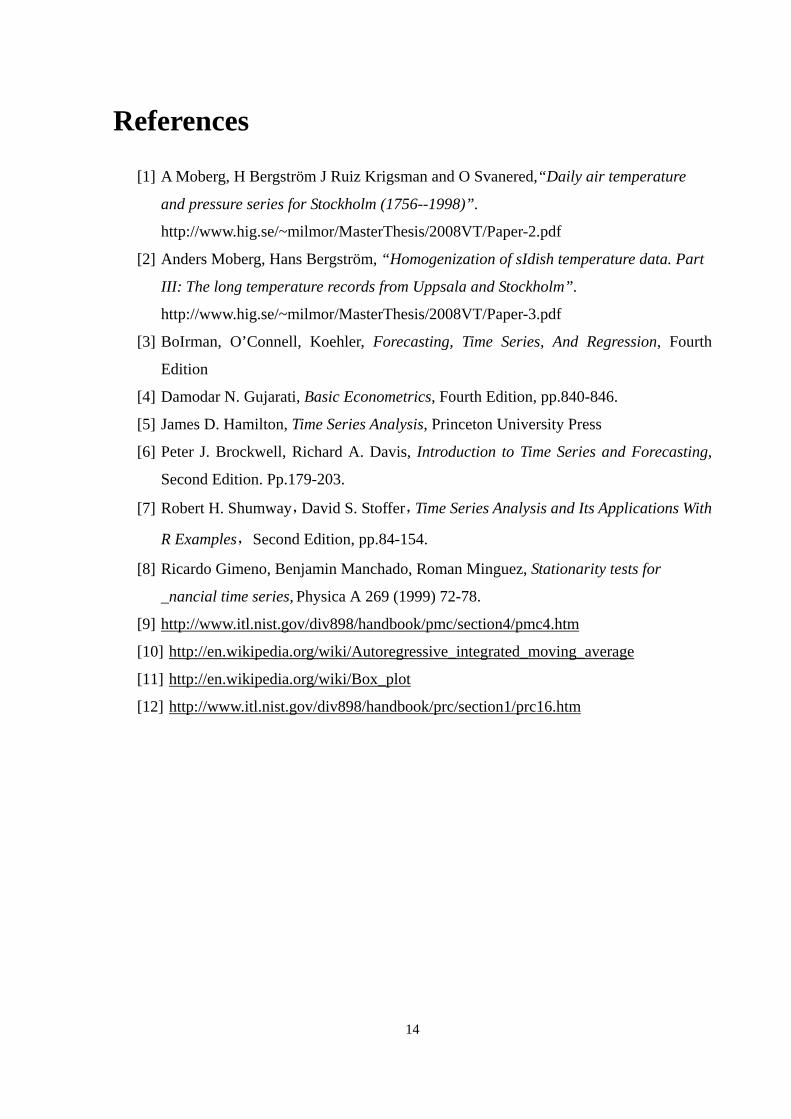
References

[1] A Moberg, H Bergström J Ruiz Krigsman and O Svanered,“Daily air temperature

and pressure series for Stockholm (1756--1998)”.

http://www.hig.se/~milmor/MasterThesis/2008VT/Paper-2.pdf

[2] Anders Moberg, Hans Bergström, “Homogenization of sIdish temperature data. Part

III: The long temperature records from Uppsala and Stockholm”.

http://www.hig.se/~milmor/MasterThesis/2008VT/Paper-3.pdf

[3] BoIrman, O’Connell, Koehler, Forecasting, Time Series, And Regression, Fourth

Edition

[4] Damodar N. Gujarati, Basic Econometrics, Fourth Edition, pp.840-846.

[5] James D. Hamilton, Time Series Analysis, Princeton University Press

[6] Peter J. Brockwell, Richard A. Davis, Introduction to Time Series and Forecasting,

Second Edition. Pp.179-203.

[7] Robert H. Shumway，David S. Stoffer，Time Series Analysis and Its Applications With

R Examples，Second Edition, pp.84-154.

[8] Ricardo Gimeno, Benjamin Manchado, Roman Minguez, Stationarity tests for

_nancial time series, Physica A 269 (1999) 72-78.

[9] http://www.itl.nist.gov/div898/handbook/pmc/section4/pmc4.htm

[10] http://en.wikipedia.org/wiki/Autoregressive_integrated_moving_average

[11] http://en.wikipedia.org/wiki/Box_plot

[12] http://www.itl.nist.gov/div898/handbook/prc/section1/prc16.htm

15

Appendix I : Tables

Table 1 an example of monthly average temperature in Stockholm (1998-2007) (°C)

Month Year

Jan Feb Mar Apr May Jun Jul Aug Sep Oct Nov Dec

1998 0.4 1.7 0.4 4 11 13.5 16.5 14.9 13 6.9 0.2 0.2

1999 -1.6 -1.6 1.6 7.5 10.1 17.2 20.2 17.1 16.1 8.1 4.7 -1

2000 -0.3 0.5 2.2 6.9 12.4 14.7 16.2 16.5 12.1 10.6 7 2.9

2001 0.1 -3.4 -0.4 5.9 11.2 15.4 20 17.4 12.7 10 3.1 -1.4

2002 -0.3 1.7 2.5 7.4 12.6 17.5 19.2 21.3 13.6 4 1 -3.4

2003 -3.1 -3.2 3.2 4.6 11.6 16.1 20.6 17.7 13.6 5.2 4.6 1.5

2004 -2.8 -0.7 1.9 6.9 10.9 14.6 17.1 18.5 13.5 7.8 1.9 1.6

2005 1.3 -1.7 -1.4 6.9 11 15.1 19.4 17 13.9 8.9 4.4 0.1

2006 -2.3 -2.7 -2.9 5.4 11.4 17 20.8 19.2 15.6 9.8 4.9 4.9

2007 0.4 -2.8 4.7 8.2 11.4 16.6 17 17.8 12.2 7.7 2.4 1.8

Table 2 summary for each month average temperature from 1756 to 2007

min max mean s.d. Jan -14.3 2.4 -3.614 2.94859 Feb -13.1 3.5 -3.611 3.20619 Mar -8.9 4.1 -1.424 2.61603 Apr -1.3 7.7 3.465 1.77067 May 3.4 12.8 8.867 1.69351 Jun 9.9 17.7 14.06 1.5412 Jul 12.3 20.7 16.74 1.67225

Aug 11.9 20.6 15.76 1.65758 Sep 8.2 15.7 11.7 1.37663 Oct 0.6 10.8 6.606 1.78511 Nov -4.9 6.6 1.658 1.8606 Dec -10.4 4.3 -1.681 2.40985

16

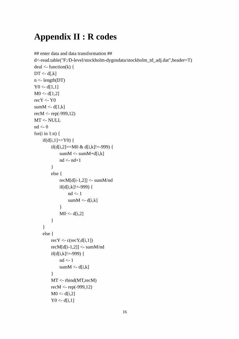
Appendix II : R codes

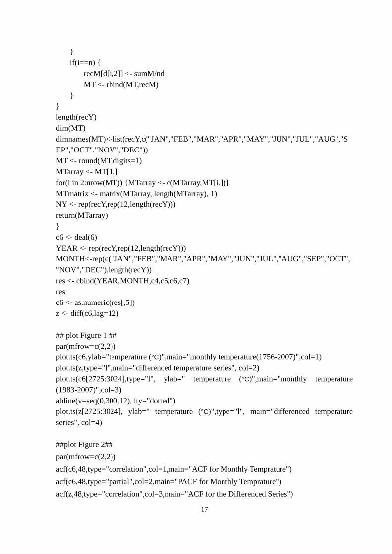
## enter data and data transformation ## d<-read.table("F:/D-level/stockholm-dygnsdata/stockholm_td_adj.dat",header=T) deal <- function(k) { DT <- d[,k] n <- length(DT) Y0 <- d[1,1] M0 <- d[1,2] recY <- Y0 sumM <- d[1,k] recM <- rep(-999,12) MT <- NULL nd <- 0 for(i in 1:n) { if(d[i,1]==Y0) { if(d[i,2]==M0 & d[i,k]!=-999) { sumM <- sumM+d[i,k] nd <- nd+1 } else { recM[d[i-1,2]] <- sumM/nd if(d[i,k]!=-999) { nd <- 1 sumM <- d[i,k] } M0 <- d[i,2] } } else { recY <- c(recY,d[i,1]) recM[d[i-1,2]] <- sumM/nd if(d[i,k]!=-999) { nd <- 1 sumM <- d[i,k] } MT <- rbind(MT,recM) recM <- rep(-999,12) M0 <- d[i,2] Y0 <- d[i,1]

17

} if(i==n) { recM[d[i,2]] <- sumM/nd MT <- rbind(MT,recM) } } length(recY) dim(MT) dimnames(MT)<-list(recY,c("JAN","FEB","MAR","APR","MAY","JUN","JUL","AUG","SEP","OCT","NOV","DEC")) MT <- round(MT,digits=1) MTarray <- MT[1,] for(i in 2:nrow(MT)) {MTarray <- c(MTarray,MT[i,])} MTmatrix <- matrix(MTarray, length(MTarray), 1) NY <- rep(recY,rep(12,length(recY))) return(MTarray) } c6 <- deal(6) YEAR <- rep(recY,rep(12,length(recY))) MONTH<-rep(c("JAN","FEB","MAR","APR","MAY","JUN","JUL","AUG","SEP","OCT","NOV","DEC"),length(recY)) res <- cbind(YEAR,MONTH,c4,c5,c6,c7) res c6 <- as.numeric(res[,5]) z <- diff(c6,lag=12) ## plot Figure 1 ## par(mfrow=c(2,2)) plot.ts(c6,ylab="temperature (°C)",main="monthly temperature(1756-2007)",col=1) plot.ts(z,type="l",main="differenced temperature series", col=2) plot.ts(c6[2725:3024],type="l", ylab=" temperature (°C)",main="monthly temperature (1983-2007)",col=3) abline(v=seq(0,300,12), lty="dotted") plot.ts(z[2725:3024], ylab=" temperature (°C)",type="l", main="differenced temperature series", col=4) ##plot Figure 2## par(mfrow=c(2,2)) acf(c6,48,type="correlation",col=1,main="ACF for Monthly Temprature") acf(c6,48,type="partial",col=2,main="PACF for Monthly Temprature") acf(z,48,type="correlation",col=3,main="ACF for the Differenced Series")

18

acf(z,48,type="partial",col=4,main="PACF for the Differenced Series") abline(v=seq(0,48,12), lty="dotted") ## stationarity test## kpss.test(c6) ###Computes the Kwiatkowski-Phillips-Schmidt-Shin (KPSS) test for the null hypothesis that x is level or trend stationary adf.test(c6) ###computes the Augmented Dickey-Fuller test for the null that 'x' has a unit root kpss.test(z) adf.test(z) ## ARIMA model for whole series ## z.fit <- arima (c6, order = c (1,0,0),seasonal = list(order = c(0,1,1),period=12) ); z.fit tsdiag(z.fit, gof.lag=12) r <- resid(z.fit) hist(r,breaks=30) qqnorm(r,pch="+") qqline(r) points(qnorm(c(.25,.75)),quantile(r,c(.25,.75)),pch=16,col=2,cex=2) ## residuals checking ## Whitenoise.test(r) Box.test(r): computes the Box-Pierce or Ljung-Box test statistic for examining the null hypothesis of independence in a given time series (stats) ##25years for each subseries ## z1 <- c6[1:324] z <- matrix ( c(rep(0,300*10)),nrow = 300,ncol = 10 ) for ( i in 2:10 ) z[,i] <- c6[(25+(i-1)*25*12):(24+i*25*12)] z2 <- z[,2] z3 <- z[,3] z4 <- z[,4] z5 <- z[,5] z6 <- z[,6] z7 <- z[,7] z8 <- z[,8] z9 <- z[,9] z10 <- z[,10]

19

## an example of ARIMA model for a subseries (1983-2007) ## acf(z10,48) pacf(z10,48) acf(diff(z10,12),48) pacf(diff(z10,12),48) z10.fit <- arima (z10, order = c (1,0,0),seasonal = list(order = c(0,1,1),period=12) ); z10.fit tsdiag(z10.fit, gof.lag=12) ## anomalies ## m <- matrix(c6,12,252) par(mfrow=c(3,4)) m1<-MT[,1] boxplot(m1) f<-fivenum(m1) ##Tukey's five number summary (minimum, lower-hinge, median, upper-hinge, maximum) mm <- m[1,] for(i in 2:12) {mm <- c(mm,m[i,])} boxplot(mm~rep(1:12,rep(252,12)), col="red", main="monthly temperature", ylab=" temperature (°C) ") lines(c(-100,100),c(0,0),col=2) r[r<f[2]+1.5*(f[2]-f[4])] r[r<f[2]+3*(f[2]-f[4])] chisq.out.test(c6, variance=var(c6), opposite = FALSE) outlier(c6, opposite = FALSE, logical = FALSE) s<-rm.outlier(c6, fill = FALSE, median = FALSE, opposite = FALSE)