Equations of the Aries Systems CodeRevision: 2/2012 by L. CarlsonCode Version: ASC v.35Code Modules: ALL modulesHistory: The code has been documented before but has failed to clearly define and reference all the

equations that reside within it. The Fusion Engineering and Design journal article by Z. Dragojlovic, et al “An Advanced Computational Algorithm for systems analysis of tokamak power plants,” FED 85 (2010) 243-265 is a starting point for the equations of the ASC.

Notes: This document attempts to account for all the equations that reside within the systems code which are hidden in and amongst all the modules. The mentality with which this is written is “How would you write the code from scratch? What equations are necessary to construct the parts of a tokamak power plant and what information do you need to build each part? What do you need from other modules? What are the references and where is the documentation found?” Costing Account Equations can be found in the document CostingAccounts.cpp.

Table of Contents

1. Physics Module Equations.....................................................................................................2

2. Building Volumes....................................................................................................................2

3. Blanket Pumping Power.........................................................................................................3

4. Divertor Pumping Power.......................................................................................................4

5. Divertor Heat Flux..................................................................................................................4

6. Power Summation and Accountability.................................................................................6

7. Gross Cycle Efficiency of the Brayton Power Conversion Cycle.....................................11

8. Current Drive........................................................................................................................12

9. Parts.......................................................................................................................................13A. Plasma Surface Area.......................................................................................................................................13B. Last Closed Magnet Surface (Sepatrix)....................................................................................................14C. First Wall IB Geometry.................................................................................................................................15D. First Wall OB Geometry...............................................................................................................................16E. Blanket IB Geometry......................................................................................................................................16F. Blanket OB Geometry.....................................................................................................................................16G. Back Wall IB Geometry (DCLL)...............................................................................................................17H. Back Wall OB Geometry (DCLL).............................................................................................................17I. Blanket II Geometry (SCLL).........................................................................................................................17J. Divertor Plates (SCLL)...................................................................................................................................18K. Divertor Plates (DCLL).................................................................................................................................19L. Replaceable HT Shield...................................................................................................................................20M. HT Shield............................................................................................................................................................21N. Skeleton Ring (DCLL)...................................................................................................................................22O. Manifold (DCLL OB and vert)...................................................................................................................22P. Manifolding (SCLL)........................................................................................................................................22Q. Vacuum Vessel (SCLL).................................................................................................................................23R. Vacuum Vessel (DCLL)................................................................................................................................24S. TF Magnet...........................................................................................................................................................26T. Bucking Cylinder............................................................................................................................................. 30

1

U. Upper Toroidal Cap on the TF Coil...........................................................................................................30V. Lower Toroidal Cap on the TF Coil..........................................................................................................31W. PF Coil Design..................................................................................................................................................32X. Cryogenic Dome..............................................................................................................................................35Y. Maintenance Port Window...........................................................................................................................36Z. Maintenance Ports............................................................................................................................................36AA. Upper Vacuum Vessel Duct.........................................................................................................................37…END of Parts…......................................................................................................................................................39

1. Physics Module EquationsReference: Z. Dragojlovic et al. 1/2010 An Advanced Computational Algorithm for systems analysis of

tokamak power plants,” FED 85 (2010) 243-265.Code Modules: inpar.txt & inpar2.txt (input files), corona (plasma equilibrium look-up table), makefile

(instructions to build the executable), PlasmaPhysics.exe (executable), runphysics.sh (run command shell), sysplas_PC.F (source code)

Notes: The author of the physics module is C. Kessel. It is the first module that is run when utilizing the Aries Systems Code. It scans the input files and creates a listing of viable physics operating points. The physics module must be compiled on a Linux machine with g++ and gfortran compilers.

The specific equations contained in the source code sysplas_PC.F are lengthy and beyond the scope of this overview document. For details regarding the equations, the author C. Kessel or the systems code administrator should be contacted. The physics module is described in detail in the physics section of the Fusion Engineering and Design journal article as referenced above. See also the Physics Module on the Documentation Homepage.

2. Building VolumesReference: Already in code, no reference.Code Modules: DesignPoint.cppNotes: Volumes are computed for costing specifications in CostingAccounts.cpp

A. Reactor Building Volume:Calculates the exterior reactor building volume in m3 from the cryodome part. vol_reactor_bldg = (pow((ksihi + 9.0), 2.0)*6.0*etahi + 1.55e5)*cATfit;

o cATfit = 138698.0/181655.0 (investigation found that 138698 is Aries-AT volume from published literature and 181655 is Prometheus-HI volume, no reference)

o ksihi = outboard max width of the cryodomeo etahi = vertical max height of the cryodome

B. Support Structure Building Volume:Approximated as 20% of the fusion power core volume. vol_str = 0.20*FPC_vol;

2

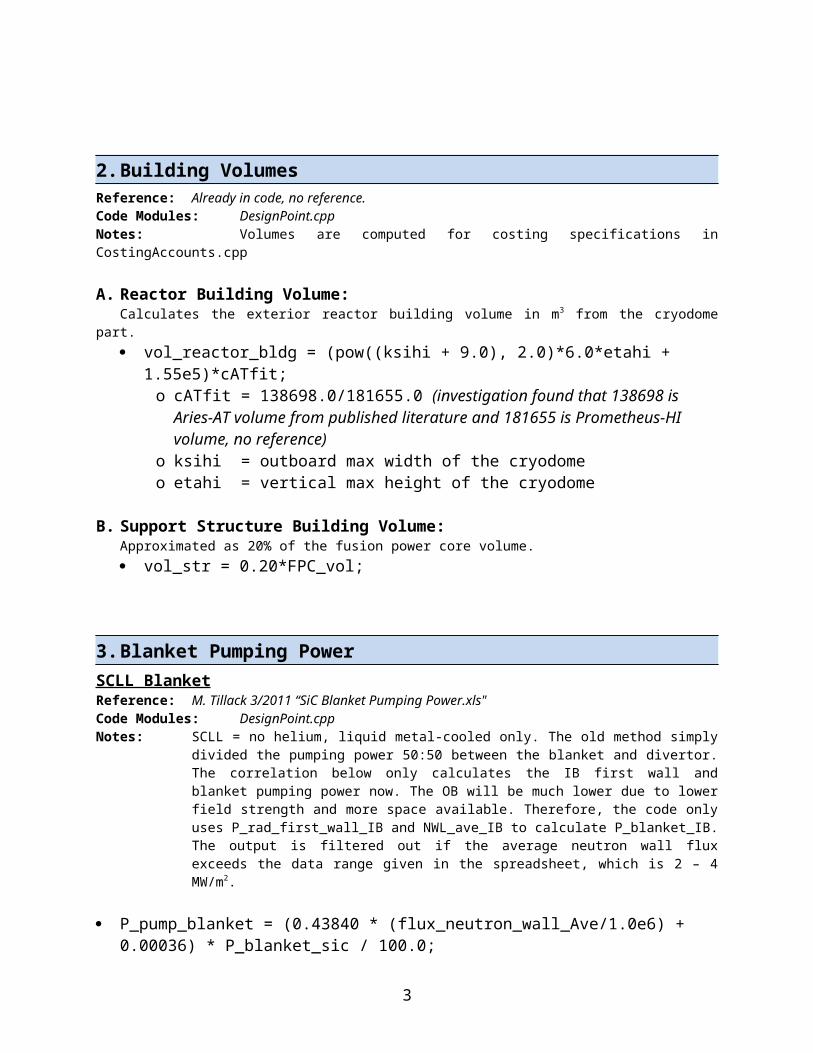
3. Blanket Pumping PowerSCLL BlanketReference: M. Tillack 3/2011 “SiC Blanket Pumping Power.xls"Code Modules: DesignPoint.cppNotes: SCLL = no helium, liquid metal-cooled only. The old method simply divided the pumping power

50:50 between the blanket and divertor. The correlation below only calculates the IB first wall and blanket pumping power now. The OB will be much lower due to lower field strength and more space available. Therefore, the code only uses P_rad_first_wall_IB and NWL_ave_IB to calculate P_blanket_IB. The output is filtered out if the average neutron wall flux exceeds the data range given in the spreadsheet, which is 2 – 4 MW/m2.

P_pump_blanket = (0.43840 * (flux_neutron_wall_Ave/1.0e6) + 0.00036) * P_blanket_sic / 100.0;

o P_rad_first_wall_IB = (f_rad_blanket_ib) * P_rad_chamb + (1.0 - f_rad_edge) * P_rad_edge * f_rad_edge_blanket_ib;

o A_FW_IB = 16.0/2.0*( (*FirstWallInb).surface_area("outer") );o flux_neutron_wall_IB = P_neutron * f_n_blanket_ib / A_FW_IB;o P_blanket_sic = (1.0 - f_alpha_div) * P_alpha_loss + f_n_blanket_ib * P_neutron *

f_nmul_fw_inboard + P_rad_first_wall_IB;o P_blanket = P_blanket_sic;o P_pump_blanket_loss = (1.0 - eta_pump_lm_mech) * P_pump_blanket /

eta_pump_lm_mech;

DCLL BlanketReference: M. Tillack 1/2011 “DCLL Blanket Pumping Power.xls"Code Modules: DesignPoint.cppNotes: SCLL = liquid-metal and helium cooling. The correlation below combines both the liquid-metal

and helium cooling, as well as the inboard and outboard pumping powers. The output is filtered out if the average neutron wall flux exceeds the data range given in the reference spreadsheet, which is 2 – 4 MW/m2.

P_pump_blanket = (0.03602*pow(flux_neutron_wall_Ave/1.0e6, 2) + 0.03056 * (flux_neutron_wall_Ave/1.0e6) + 0.38359) * P_blanket_dcll/100.0;

o P_blanket_dcll = (1.0 - f_alpha_div) * P_alpha_loss + (f_n_blanket_ib) * P_neutron * f_nmul_fw_inboard + (f_n_blanket_ob) * P_neutron * f_nmul_fw_outboard + P_rad_first_wall; // both IB+OB

// Need coolant fractional power split for DCLL blanket pump losses (LM pump vs He-blower); M. Tillack’s spreadsheet has PbLi 62.3%, He 37.7%o double f_pump_PbLi = 0.623;o double f_pump_He = 0.377;o P_pump_blanket_loss = ((1.0 - eta_pump_lm_mech) * f_pump_PbLi +

(1.0 - eta_pump_he) * f_pump_He) *P_pump_blanket / ((eta_pump_he + eta_pump_lm_mech)/2);

3

4. Divertor Pumping PowerReference: M. Tillack, X. Wang, "Divertor Pumping Powers - ppcompare2.xls" Dec. 2010Code Modules: DesignPoint.cppNotes: This calculates the pumping power requirement for the divertor in use. The divertor in use is

selected from the input file Setup.data. Note that P_thermal_divertor is used, not the overall P_thermal. The output is filtered if the maximum heat flux on the divertor is less than 5 or greater than 15 MW/m2, which is the range of the tabulated reference data.

P_thermal_divertor = P_alpha_loss * f_alpha_div+ P_neutron * f_n_div * f_nmul_divertor+ P_rad_edge * f_rad_edge+ P_rad_chamb * f_rad_div+ P_cond_div;

P_pump_divertor = pumping_power_divertor(flux_divertor_Max) * P_thermal_divertor/100.0;

P_pump_divertor_loss = (1.0 - eta_pump_he) * P_pump_divertor/eta_pump_he;

1. T-tube design: J. Burke’s T-Tube 2010 divertor design pumping power curve. Linear-taper with fixed slot width of 0.45 mm, inlet temp 600C, outlet 677C, P = 10 MPa; surface heat flux (MW/m^2) vs P_pump/P_thermal (%). ppttube = 0.05594 * pow(flux_divertor_Max/1.0e6,2) + 0.04931 *

(flux_divertor_Max/1.0e6) - 0.08702;

2. Plate design: X. Wang’s plate divertor design (HCFP). Helium-cooled flat plate, inlet temp 600C, outlet 677C, P = 10 MPa. ppplate = 0.0392 * pow(flux_divertor_Max/1.0e6,3) - 0.743 *

pow(flux_divertor_Max/1.0e6,2) + 5.44 * (flux_divertor_Max/1.0e6) - 11.1;

3. Combined plate-finger design: X. Wang’s finger divertor design (HCPF). Helium-cooled combined plate and finger, inlet temp 600C, outlet 700C, P = 10 MPa. ppfinger = 0.0335 * pow(flux_divertor_Max/1.0e6,2) + 0.22 * (flux_divertor_Max/1.0e6)

- 0.892;

5. Divertor Heat FluxMax Heat Flux on DivertorReference: C. Kessel, existing code, no specific reference. Edited “adivo” and “adivi” with C. Kessel 1/2011Code Modules: DesignPoint.cppNotes: Find the maximum heat flux incident on the divertor. This section of the code stems from C.

Kessel’s sysengr.f systems code. The output is filtered if the maximum heat flux on the divertor is > 8 MW/m2.

Definitions:o sym = 1.0 for up-down symmetric, 0.0 for up-down asymmetrico facdiv = factor for splitting power if up-down symmetric or noto adivo = area in outboard divertor slot for absorbing radiated power

4

o adivi = area in inboard divertor slot for absorbing radiated powero fdivrad = total radiated power fraction in divertoro fdivcondo = fraction of conducted power to divertor going to the outboardo fdivcondi = fraction of conducted power to divertor going to the inboardo fdivrado = fraction of radiated power to divertor going to the outboardo fdivradi = fraction of radiated power to divertor going to the inboardo fluxexpo = poloidal mag. flux exp. on outboard from midplane to divertor targeto fluxexpi = poloidal mag. flux exp. on inboard from midplane to divertor targeto pdiv = total power going to divertorso pdivrad = total power radiated in divertorso pdiv2 = total power conducted to divertorso pdiv2o = power conducted to outboard divertoro pdiv2i = power conducted to inboard divertoro pdivrado = power radiated in outboard divertoro pdivradi = power radiated in inboard divertoro pdivtoto = conducted + radiated power in outboard divertoro pdivtoti = conducted + radiated power in inboard divertoro den = density factor in power scrape-off formulao xlam = power scrape-off layer width at plasma midplaneo qpeakcondo = peak conducted power heat flux to outboard divertoro qpeakcondi = peak conducted power heat flux to inboard divertoro qpeakrado = peak radiated power heat flux to outboard divertoro qpeakradi = peak radiated power heat flux to inboard divertoro f_greenwald = greenwald fractiono Bt = toroidal magnetic field at plasma major radiuso Aip = plasma currento Qmhd = qmhd

Equations: if(sym == 1.0) { facdiv = 0.65; } else { facdiv = 1.00; } Rmaj = plasma_major_radius(); Asp = plasma_major_radius()/plasma_minor_radius(); adivo = 2.*pi*(Rmaj -((Rmaj/Asp)/2.0))*2.0*(Rmaj/(Asp*2.0)); adivi = 2.*pi*(Rmaj-(Rmaj/Asp))*2.0*(Rmaj/(Asp*4.0)); P_div = (P_plasma - P_rad_first_wall)/1.e6; P_div_rad = f_div_rad*P_div; P_div_2 = P_div - P_div_rad; P_div_2_o = facdiv*fdivcondo*P_div_2; P_div_2_i = facdiv*fdivcondi*P_div_2; P_div_rad_o = facdiv*fdivrado*P_div_rad; P_div_rad_i = facdiv*fdivradi*P_div_rad; den = f_greenwald*(Aip/pi*pow(Rmaj/Asp, 2.0))*0.35; xlam = 2.9e-2*2.5*pow(Qmhd, 0.75)*pow(den, 0.15)/(pow(P_div_2_o,

0.4)*Bt); // power scrape off width Q_peak_cond_o = P_div_2_o/(2.0*pi*(Rmaj-((Rmaj/Asp)/2.0))*fluxexpo*xlam);

5

Q_peak_cond_i = P_div_2_i/(2.0*pi*(Rmaj-(Rmaj/Asp)) *fluxexpi*xlam); Q_peak_rad_o = P_div_rad_o/adivo; Q_peak_rad_i = P_div_rad_i/adivi; Q_peak_tot_o = Q_peak_cond_o + Q_peak_rad_o; Q_peak_tot_i = Q_peak_cond_i + Q_peak_rad_i; get_divertor_loads(Q_peak_tot_i*1.e6, Q_peak_tot_o*1.e6); // Get's peak divertor

loads from a simple comparison flux_divertor_Max = max(Q_peak_tot_o, Q_peak_tot_i)*1.e6;

6. Power Summation and AccountabilityReference: This already existed in the code; L. Carlson added accounting for losses and verified power

balance 8/2011.Code Modules: DesignPoint.cpp, powerflow.data input fileNotes: These equations describe the net electric power and power losses. See also the Power Flow

Diagram on the Documentation Homepage for a visual representation. There is a check in the code to ensure that the power generated is equal to the net electric power plus the unrecoverable power lost through heat, friction, or inefficiencies.

Definitions:Power Conversion Factors (from powerflow.data input file)o f_alpha_loss = fraction of loss of alfa particles; = 0 for tokamako f_alpha_div = fraction of alpha loss to divertoro f_div_rad = fraction of edge radiation from particleso f_rad_edge = fraction of edge radiation to divertor

Fraction of edge radiation to FWBS = (1.0 - f_rad_edge); IB/OB split of edge radiation to FWBS is dependent on FW area

o f_rad_edge_blanket_ib = (*FirstWallInb).surface_area("outer") / ((*FirstWallInb).surface_area("outer") + (*FirstWallOutb).surface_area("outer"));

o f_rad_edge_blanket_ob = (1.0 - f_rad_edge_blanket_ib);

Neutron Energy Multiplication (all M = 1.1 for now)o f_nmul_fw_inboard = FW/blanket IBo f_nmul_fw_outboard = FW/blanket OBo f_nmul_shield_inboard = shield IBo f_nmul_shield_outboard = shield OBo f_nmul_divertor = divertor plateso f_nmul_div_blanket = blanket behind divertoro f_nmul_div_shield = shield behind divertor

Efficiency of Pumps – He, liquid-metal MHD, liquid-metal mechanicalo eta_pump_he = efficiency of the He pump/blowero eta_pump_he_recovered = fraction of heat recoverableo eta_pump_lm_mhd = efficiency of the Liquid Metal MHD pumpo eta_pump_lm_mhd_recovered = fraction of heat recoverable

6

o eta_pump_lm_mech = efficiency of the Liquid Metal mechanical pumpo eta_pump_lm_mech_recovered = fraction of heat recoverable

PowersPower from Neutron Particles P_alpha = inputdata[npt][53]*1.0e6; // alpha power contained in plasma P_neutron = 4.0*P_alpha; P_fusion = P_alpha + P_neutron; // P_fusion = 5*P_alpha

Auxiliary PowerL. El-Guebaly recommends 65 MW = 30 misc + 35 MW cryo load (Dec 2010), scaling from ITER. Also recommends 2 MW for low temperature superconductor and 0.5 MW for high temperature SC P_aux_func = power to auxiliary functions P_cryo = cryogenic magnet power

Plasma Heating Power eta_plasma_heating = aux. power into plasma for power balance P_aux_for_power_balance = (inputdata[npt][26]) * 1.0e6; // incl. CD power P_plasma_heating = P_aux_for_power_balance - P_cd_generic; // MW P_plasma_heating_loss = (1.0 - eta_plasma_heating) * P_plasma_heating /

eta_plasma_heating;

Power Radiated from ChamberBremsstralhlung radiation + Cyclotron power + Line radiation P_rad_chamb = (inputdata[npt][22] + inputdata[npt][27] + inputdata[npt][29])*1.0e6;

Current Drive PowerCurrent drive power is listed in its own section titled “Current Drive.”

Power From Alpha ParticlesIf there is any alpha loss, it would go into the FW and be recovered as heat P_alpha_loss = f_alpha_loss * P_alpha; // = 0 for a tokamak P_transport = P_alpha - P_alpha_loss; P_plasma = P_transport + P_aux_for_power_balance; // in MW P_particle = P_plasma - P_alpha_loss - P_rad_chamb; P_rad_edge = f_div_rad * P_particle; // Edge radiation power P_cond_div = (1.0 - f_div_rad) * P_particle; // Edge conducted power

Average Neutron Wall Flux “NWL_ave”C.Kessel: neutron wall load = 4/5*Pfusion/plasma_SA = P_neutron/A_plasma_surface. Neutron wall loading expresses the neutron wall flux against the wall divided by the surface area of the plasma.

flux_neutron_wall_Ave = P_neutron/A_plasma_surface; // area of plasma surface is found “Plasma” section

flux_neutron_wall_Ave_w_SOL = P_neutron/A_plasma_surface_w_SOL;

7

Maximum Neutron Wall Flux Using Peaking FactorTwo tables, one for SCLL and one for DCLL blanket, give peaking factors depending on plasma aspect ratio. If the aspect ratio is not found in the table, then the code interpolates. L. El-Guebaly updated 5/2011 at project meeting.

DCLL: at A = 1.6, PF = 1.94; at A = 4.0, PF = 1.5 SCLL: at A = 1.7, PF = 2.0; at A = 4.0, PF = 1.55 flux_neutron_wall_Max = flux_neutron_wall_Ave * peaking_factor;

Heat Flux to First Wall IB + OB (Average and Maximum): L. Carlson changed old geometric factor (1.0-f_geo_div) to f_rad_blanket_ib + f_rad_blanket_ob. This has increased P_rad_first_wall as well as flux_heat_wall.

P_rad_first_wall = (f_rad_blanket_ib + f_rad_blanket_ob) * P_rad_chamb + (1.0 - f_rad_edge) * P_rad_edge;

flux_heat_wall_Ave = P_rad_first_wall / A_first_wall; // Average heat flux on the wall flux_heat_wall_Max = 1.25 * flux_heat_wall_Ave; // Maximum heat flux on the wall

Neutron Power DistributionNeutron power distribution from plasma given from Laila, read from powerflow.data. "For A=4, 10% of power is deposited in divertor, 25% in IB blanket, and 65% in OB.

f_n_div = fraction of neutron power from plasma to divertor (A=4) f_n_blanket_ib = fraction of neutron power from plasma to IB blanket f_n_blanket_ob = fraction of neutron power from plasma to OB blanket

Radiated power distribution from plasma:Estimated by M. Tillack, read from powerflow.data input file.

f_rad_div = fraction of radiated power from plasma to divertor f_rad_blanket_ib = fraction of radiated power from plasma to IB blanket f_rad_blanket_ob = fraction of radiated power from plasma to OB blanket

Power AbsorbedA. FWBS (First-wall, blanket, shield): Set up array:

P_FWBSGroup[2][2][2]; neutron = 0; // i's condRad = 1; fw_blanket = 0; // j's

shield = 1; outboard = 0; // k's inboard = 1;

P_lm_pump_recovered = P_pump_blanket; // LM mechanical pump’s thermal contribution

P_neutron_FWBSGroup_in = (f_n_blanket_ib + f_n_blanket_ob) * P_neutron; P_neutron_FWBSGroup_ib = f_n_blanket_ib * P_neutron; P_neutron_FWBSGroup_ob = f_n_blanket_ob * P_neutron;

P_condRad_FWBSGroup_in = (1.0 - f_alpha_div) * P_alpha_loss+ (f_rad_blanket_ib+f_rad_blanket_ob) * P_rad_chamb

8

+ (1.0 - f_rad_edge) * P_rad_edge;

// Conduction + radiation powers are split here. They do not get deposited in the shield, only in the FW and blanket, which are the surface layers exposed to plasma. P_FWBSGroup[condRad][fw_blanket][outboard] = f_rad_blanket_ob * P_rad_chamb + (1.0

- f_rad_edge) * P_rad_edge * f_rad_edge_blanket_ob; P_FWBSGroup[condRad][fw_blanket][inboard] = (1.0 - f_alpha_div) * P_alpha_loss +

f_rad_blanket_ib * P_rad_chamb + (1.0 - f_rad_edge) * P_rad_edge * f_rad_edge_blanket_ib;

P_FWBSGroup[condRad][shield][outboard] = 0.0; P_FWBSGroup[condRad][shield][inboard] = 0.0;

// Split the IB & OB powers from neutrons into FW/blanket and shield fractions. Include the effect of neutron energy multiplication (1.1).

f_fw_blanket = 0.90; // from powerflow.data input filef_shield = 0.10; // from powerflow.data input file

P_FWBSGroup[neutron][fw_blanket][outboard] = f_fw_blanket * f_nmul_fw_outboard * P_neutron_FWBSGroup_ob;

P_FWBSGroup[neutron][fw_blanket][inboard] = f_fw_blanket * f_nmul_fw_inboard * P_neutron_FWBSGroup_ib;

P_FWBSGroup[neutron][shield][outboard] = f_shield * f_nmul_shield_outboard * P_neutron_FWBSGroup_ob;

P_FWBSGroup[neutron][shield][inboard] = f_shield * f_nmul_shield_inboard * P_neutron_FWBSGroup_ib;

Power AbsorbedB. Divertor: Set up array:

P_DivGroup[3][4]; divPlates = 0; // j's divBlanket = 1; divShield = 2;

double P_he_pump_recovered = P_pump_divertor; // He pump’s thermal contribution

double P_neutron_DivGroup_in = f_n_div * P_neutron; // M applied below

double P_condRad_DivGroup_in = f_alpha_div * P_alpha_loss + f_rad_div * P_rad_chamb + f_rad_edge * P_rad_edge + P_cond_div;

// Conduction and radiation powers are only deposited in the divertor plates. P_DivGroup[condRad][divPlates] = P_condRad_DivGroup_in; P_DivGroup[condRad][divBlanket] = 0.0;

9

P_DivGroup[condRad][divShield] = 0.0;

// Split the power from neutrons into fractions that go into divertor plates, blanket behind divertor and shield behind divertor. Include the effect of neutron energy multiplication. (TBD low temperature components, i.e. vacuum vessel, 1%?) double f_div_plates = 0.50; // from powerflow.data input file double f_div_blanket = 0.40; // from powerflow.data input file double f_div_shield = 0.10; // from powerflow.data input file

P_DivGroup[neutron][divPlates] = f_div_plates * f_nmul_divertor * P_neutron_DivGroup_in;

P_DivGroup[neutron][divBlanket] = f_div_blanket * f_nmul_div_blanket * P_neutron_DivGroup_in;

P_DivGroup[neutron][divShield] = f_div_shield * f_nmul_div_shield * P_neutron_DivGroup_in;

Thermal Power SummationA. FWBS (First-wall, blanket, shield): for(int i=0; i<2; i++) { for(int j=0; j<2; j++) { for(int k=0; k<2; k++) { P_thermal = P_thermal + P_FWBSGroup[i][j][k]; P_thermal_fwbs = P_thermal_fwbs + P_FWBSGroup[i][j][k];

B. Divertor: for(int i=0; i<2; i++) { for(int j=0; j<3; j++) { P_thermal = P_thermal + P_DivGroup[i][j]; // continue to add to P_thermal P_thermal_div = P_thermal_div + P_DivGroup[i][j]; } }

P_thermal_fwbs = P_thermal_fwbs + P_lm_pump_recovered; // recovered power form above

P_thermal_div = P_thermal_div + P_he_pump_recovered; P_thermal = P_thermal_fwbs + P_thermal_div; // total P_thermal

Power Flow Accountability: P_net_electric = P_gross_electric –

P_plasma_heating / eta_plasma_heating – P_cd_generic / eta_cd_generic –P_aux_func –P_cryo –P_pump_blanket / eta_pump_lm_mech – P_pump_divertor / eta_pump_he;

P_generation = P_fusion*(0.8*M + 0.2)/1.0e6; // M = neutron mult. factor, usually = 1.1

10

P_losses = P_plasma_heating_loss +P_cd_loss +P_brayton_loss + P_pump_blanket_loss + P_pump_divertor_loss + P_aux_func + P_cryo; //+ LT_fwbs_loss, + LT_div_loss // to be added

P_leftover = P_generation - (P_net_electric/1.0e6) - (P_losses/1.0e6); P_leftover should be = 0 if all power flow is accounted for

7. Gross Cycle Efficiency of the Brayton Power Conversion CycleReference: R. Raffray, 8/2010 "Raffray - Pumping Power systems code input.xls"; polynomial fits added by L.

Carlson 5/2011.M. Tillack concluded 11/2010 that we can continue to use R. Raffray's NWL vs cycle efficiency for the near term since our NWL_max and q" are low (~4.2 MW/m^2, ~0.25 MW/m^2 for ~AT).

Code Modules: DesignPoint.cppNotes: This calculates the gross cycle efficiency of the Brayton power conversion cycle. It takes the

maximum neutron wall loading in MW/m2 at the first wall for different surface heat fluxes (q’’max) in MW/m2 and returns the gross cycle efficiency Q.

1. DCLL: Choose polynomial fit depending on q’’ if (q2 < 0.250) { eta = 0; cout << "Maximum surface heat flux q'' is too low for the

Brayton cycle tabulated interval " << q2 << "\n"; } if (q2 >= 0.250 && q2 <= 0.500) { eta = 0.00013*pow(nwl2,3) - 0.00190*pow(nwl2,2) +

0.00087*nwl2 + 0.44578; if (nwl2 < 2.0 && nwl2 > 7.5) cout << "Maximum neutron wall load (NWL_max) at first

wall is out of the Brayton cycle tabulated interval " << nwl2 << "\n"; } if (q2 > 0.500 && q2 <= 0.750) { eta = 0.00002*pow(nwl2,3) - 0.00009*pow(nwl2,2) -

0.00814*nwl2 + 0.45770; if (nwl2 < 2.4 && nwl2 > 7.5) cout << "Maximum neutron wall load (NWL_max) at first

wall is out of the Brayton cycle tabulated interval " << nwl2 << "\n"; } if (q2 > 0.750 && q2 <= 1.000) { eta = 0.00018*pow(nwl2,3) - 0.00275*pow(nwl2,2) +

0.00599*nwl2 + 0.43195; if (nwl2 < 4.5 && nwl2 > 7.5) cout << "Maximum neutron wall load (NWL_max) at first

wall is out of the Brayton cycle tabulated interval " << nwl2 << "\n"; } if (q2 > 1.000 && q2 <= 1.250) { eta = -0.00031*pow(nwl2,2) + 0.00290*nwl2 +

0.38929; if (nwl2 < 4.8 && nwl2 > 7.5) cout << "Maximum neutron wall load (NWL_max) at first

wall is out of the Brayton cycle tabulated interval " << nwl2 << "\n"; } if (q2 > 0.750) { eta = 0; cout << "Maximum surface heat flux q'' (" << q2 << ") is too

high for the Brayton cycle tabulated interval.\n";}

2. SCLL: Choose polynomial fit depending on q’’

11

if (q2 < 0.250) { eta = 0; cout << "Maximum surface heat flux q'' is too low for the Brayton cycle tabulated interval " << q2 << "\n"; }

if (q2 >= 0.250 && q2 <= 0.375) { eta = -0.00347*nwl2 + 0.58859; if (nwl2 < 1.5 && nwl2 > 6.0) cout << "Maximum neutron wall load (NWL_max) at first

wall is out of the Brayton cycle tabulated interval " << nwl2 << "\n"; } if (q2 > 0.375 && q2 <= 0.500) { eta = -0.00361*nwl2 + 0.56934; if (nwl2 < 1.8 && nwl2 > 6.0) cout << "Maximum neutron wall load (NWL_max) at first

wall is out of the Brayton cycle tabulated interval " << nwl2 << "\n"; } if (q2 > 0.500 && q2 <= 0.625) { eta = -0.00362*nwl2 + 0.54828; if (nwl2 < 2.4 && nwl2 > 6.0) cout << "Maximum neutron wall load (NWL_max) at first

wall is out of the Brayton cycle tabulated interval " << nwl2 << "\n"; } if (q2 > 0.625 && q2 <= 0.750) { eta = -0.00363*nwl2 + 0.52605; if (nwl2 < 3.0 && nwl2 > 6.0) cout << "Maximum neutron wall load (NWL_max) at first

wall is out of the Brayton cycle tabulated interval " << nwl2 << "\n"; } if (q2 > 0.750) { eta = 0; cout << "Maximum surface heat flux q'' (" << q2 << ") is too

high for the Brayton cycle tabulated interval.\n";}

8. Current DriveReference: R. Raffray, "Power Flow.doc” 5/2008, implemented into code by Z. Dragojlovic; See also L.

Waganer “Cost Basic Documentation (11-25-10).doc” for updated costing to 2009$.Code Modules: DesignPoint.cppNotes: The current drive parameters are called by reading part of the powerflow.data input file. This

defines parameters such as efficiencies, frequencies, and unit costs of potential CD units such as lower hybrid (LH), neutral beam (NB), and fast wave (FW). The CD efficiencies are interpolated if the value is not directly found in the table. The frequency is set in the input file as well.

CD Frequency, Efficiency, Cost TableThe following table gives the efficiency and cost at the frequency for an ICRF Fast Wave current drive design.

frequency[6] = {80.0e6, 158.0e6, 250.0e6, 800.0e6, 2500.0e6, 8000.0e6}; efficiency[6] = {0.84, 0.72, 0.65, 0.63, 0.48, 0.44 }; unit_cost[6] = {1.15, 1.15, 2.30, 2.30, 2.30, 2.87 }; // 1992$ unit_cost[6] = {1.65, 1.65, 3.29, 3.29, 3.29, 3.29 }; // 2009$

Generic current drive efficiencies eta_cd_generic = generic current drive source efficiency eta_cd[nb] = generic NB current drive source efficiency eta_cd[lh] = generic LH current drive source efficiency eta_cd[icrf] = generic ICRF current drive source efficiency eta_cd[ec] = generic EC current drive source efficiency

Current Drive Power P_cd_generic = inputdata[npt][25]*1.0e6; // from physics input file P_cd_loss = (1.0 - eta_cd_generic)*P_cd_generic/eta_cd_generic;

12

9. PartsReference: Existing codeCode Modules: Geometry.cppNotes: The following sections contain information on how to build the various parts of the tokamak

power plant. Most dimensions are read into the code from the builds_generic.data input files. More information about the inputs and outputs can be found in ASC Inputs & Outputs.pdf on the Documentation page. More information about what is contained in the Geometry.cpp module can be found in the document ASC Geometry Module.pdf.

A. Plasma Surface AreaReference: C. Kessel 5/2011 “Plasma Contour2 – Kessel plasma geometry discretized formulas.pdf”Code Modules: Geometry.cpp “1/2 Plasma Geometry – at plasma surface” & “2/2 Plasma Geometry – with SOL

attached.”Notes: Calculates the surface area of the plasma. The average neutron wall flux uses this by dividing the

neutron power by the plasma surface area.

A. Elliptical equations: Good for estimation but not accurate when plasma elongation, squareness, and triangularity push the plasma shape beyond an ellipse. A_plasma_surface = 4.0*pi*pi*R * (R / A + SOL) * sqrt((1.0 + pow(k, 2.0))/ 2.0);

o SOL = SOL thickness from input fileo A = aspect ratio from physics module outputo k = kappa, plasma elongationo R = plasma major radius

B. Perimeter method: Uses the perimeter function in Part.cpp to find the plasma’s perimeter and then revolve it about 2R.[from ASC Part.cpp module] A_plasma_surface =

(*Plasma).surface_area("plasma_perimeter")*2.0*pi*plasma_major_R;

C. Discretized equations: These take into account all the plasma factors that affect its size. This is the most accurate formula and is currently used in the code. To take advantage of symmetry, the contour shape is multiplied by two. R = Ro + a cos(ϑ + sin-1(δ) sin(ϑ)) Z = a κ sin(ϑ + ςo sin(2ϑ)) for ϑ < π/2 Z = a κ sin(ϑ + ςi sin(2ϑ)) for ϑ > π/2

o Ro = plasma major radiuso a = plasma minor radius (add SOL thickness here to find surface area incl. SOL)o κ = plasma elongationo δ = plasma triangularityo ςo = plasma squareness on outboard side (~0)o ςi = plasma squareness on inboard side (~0)o ϑ = poloidal angle

13

B. Last Closed Magnet Surface (Sepatrix)Reference: Z. Dragojlovic, C. Kessel 2/2007 “X-Point.pdf”Code Modules: Geometry.cpp “Last Closed Magnetic Surface”Notes: Also known as “LCMSurf” or “Sepatrix.” The last closed magnetic surface follows the contour of

the plasma shape offset by the thickness of the SOL. It separates from the plasma at the top and bottom and crosses in the middle of the divertor region.

Reference Part: plasma boundary

How to BuildThe departure angles from following the plasma, alphain and alphaout, are taken from CAD drawings of ARIES-AT. alphain = 66.25*pi/180.0; // = 1.156 rad alphaout = pi - 19.44*pi/180; // = 2.802 rad delta = (*Machine).inboard_generic_build(0)/2.0; // distance between plasma surface and

separatrix = 1/2 * SOL

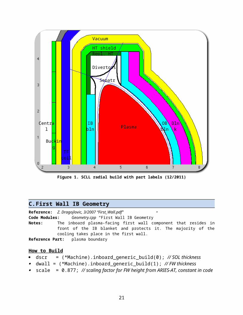
Build the sepatrix from contour lines by following the plasma boundary. Space the sepatrix at ½ the scrape-off-layer thickness away from the plasma (“delta”). Follow the plasma boundary up until the vector of the sepatrix is equal to the above constants, alphain and alphaout, which mimic the angles from ARIES-AT. Terminate the lines when then hit the replaceable HT shield. See Figure 1 for more details.

14

Figure 1. SCLL radial build with part labels (12/2011)

C. First Wall IB GeometryReference: Z. Dragojlovic, 3/2007 “First_Wall.pdf”Code Modules: Geometry.cpp “First Wall IB Geometry”Notes: The inboard plasma-facing first wall component that resides in front of the IB blanket and protects

it. The majority of the cooling takes place in the first wall.Reference Part: plasma boundary

How to Build dscr = (*Machine).inboard_generic_build(0); // SOL thickness dwall = (*Machine).inboard_generic_build(1); // FW thickness scale = 0.877; // scaling factor for FW height from ARIES-AT, constant in code

Build the IB first wall at thickness “dwall” from input file and height scaled from ARIES-AT design, 0.877*plasma height. Place the IB FW a distance equal to the SOL from the plasma.

HT shield

Vacuum vessel

Repl. HT shield

TFcoil

Divertors

PlasmaIB

blnk

Sepatrix

Central solenoid

Bucking cylinder

OBblnk

Blnk II

15

D. First Wall OB GeometryReference: Z. Dragojlovic, 3/2007 “First_Wall.pdf”Code Modules: Geometry.cpp “First Wall OB Geometry”Notes: The outboard plasma-facing first wall component that resides in front of the OB blanket and

protects it. The majority of the cooling takes place in the first wall.Reference Part: plasma boundary

How to Build dscr = (*Machine).inboard_generic_build(0); // SOL thickness dwall = (*Machine).inboard_generic_build(1); // FW thickness scale = 0.34833; // constant from First Wall.doc to scale geometrically to AT (ref?) scale2 = 1.2577; // constant from First Wall.doc to scale geometrically to AT (reference?

The First_Wall.pdf has this number in the document with an explanation that it is used to scale to the AT design, but how the specific number was attained.)

Build the OB first wall at thickness “dwall,” which is taken from input file. Follow the plasma upward on the OB side a distance equal to the SOL from the plasma and end at the height of the plasma reference. From here, go vertical upward from the height of the plasma + 1.2577, which is a scaling factor from the ARIES-AT design. This allows room for the divertors on the top and bottom of the double-null plasma.

E. Blanket IB GeometryReference: Z. Dragojlovic, 3/2007 “Blanket.pdf”Code Modules: Geometry.cpp “Blanket IB Geometry”Notes: Extends nearly the length of the plasma behind the first wall and provides bulk cooling and

neutron shielding with either PbLi and/or helium.Reference Part: inboard first wall

How to Build gap = 0.0; // gap between the FW and blanket dwall = (*Machine).inboard_generic_build(2); // blanket thickness from radial build

Build the IB blanket at thickness “dwall” by referencing the IB first wall. Extend it to the same height as the IB first wall.

F. Blanket OB GeometryReference: Z. Dragojlovic, 3/2007 “Blanket.pdf”Code Modules: Geometry.cpp “Blanket OB Geometry”Notes: Extends around the outboard portion of the plasma and provides bulk cooling and neutron

shielding with either PbLi and/or helium.Reference Part: outboard first wall

How to Build dfw = (*Machine).outboard_generic_build(1); // FW I thickness

16

gap = 0.0; // FW I to blanket gap dwall = (*Machine).outboard_generic_build(2); // OB blanket I thickness

Build the OB blanket at thickness “dwall” by referencing the OB first wall. Extend it to the same height as the OB first wall.

G. Back Wall IB Geometry (DCLL)Reference: No specific documentationCode Modules: Geometry.cpp “Back Wall IB Geometry (DCLL)”Notes: Essentially a thinner “IB First Wall” behind the IB blanket that follows the same contour but with

a different composition.Reference Part: inboard blanket

How to Build gap = (*Machine).inboard_generic_build(5); // blanket and back wall gap dwall = (*Machine).inboard_generic_build(6); // back wall thickness

Build the IB back wall at thickness “dwall” behind the IB blanket by referencing the IB blanket. Extend it to the same height as the IB blanket/first wall.

H. Back Wall OB Geometry (DCLL)Reference: No specific documentationCode Modules: Geometry.cpp “Back Wall OB Geometry (DCLL)”Notes: Essentially a thinner “OB First Wall” behind the OB blanket that follows the same contour but

with a different composition.Reference Part: outboard blanket

How to Build dblanket = (*Machine).outboard_generic_build(2); // blanket I thickness gap = 0.0; // blanket I to back wall II gap dwall = (*Machine).outboard_generic_build(9); // back wall II thickness

Build the OB back wall at thickness “dwall” behind the OB blanket of thickness “dblanket” by referencing the IB blanket. Extend it to the same height as the OB blanket/first wall.

I. Blanket II Geometry (SCLL)Reference: No specific documentationCode Modules: Geometry.cpp “Blanket OB Geometry”Notes: Second blanket behind the main OB blanket in the SCLL design. Provides additional bulk cooling

and neutron shielding with either PbLi and/or helium. Not used in DCLL design.Reference Part: outboard blanket

17

How to Build dwref = (*Machine).outboard_generic_build(2); // OB blanket thickness dwgap = (*Machine).outboard_generic_build(6); // OB blanket and blanket II gap

(stabilizing shell?) dwall = (*Machine).outboard_generic_build(8); // blanket II thickness

Build the OB blanket II at thickness “dwall” by referencing the OB blanket. Extend it to the same height as the OB blanket. Blanket II has a different composition than blanket I.

J. Divertor Plates (SCLL)Reference: Z. Dragojlovic, 3/2007 “Divertor_Plates.pdf”Code Modules: Geometry.cpp “Divertor Plates (SCLL)”Notes: This part design builds the six divertor plates in the upper and lower divertor region. Note that the

reference document uses scaling factors to scale the divertors to the ARIES-AT design, whereas the code has implemented the scaling of normalized vectors instead.

Reference Parts:o LCMSurf = Sepatrixo RefLeft = Inboard blanketo RefRight = Outboard blanket

How to Build delta = (*Machine).inboard_generic_build(0)/10.0; // 1/10th SOL dwall = (*Machine).inboard_generic_build(2); // IB blanket thickness drephts = (*Machine).vertical_generic_build(3); // repl HT shield thickness

Implement the curvature identical to the ARIES-AT divertor plates by stretching the normalized vectors which sample this curvature between the calculated end-points of the divertor plates generated by this code.

Normalized sample vectors: (same as DCLL below; no reference) xnorm0[10] = {0.0, 0.01, 0.01, 0.03, -0.02, -0.17, -0.35, -0.56, -0.76, -1.0}; ynorm0[10] = {0.0, 0.17, 0.31, 0.45, 0.57, 0.69, 0.79, 0.86, 0.93, 1.0};

xnorm1[10] = {0.0, 0.09, 0.24, 0.37, 0.51, 0.67, 0.81, 0.92, 0.98, 1.0}; ynorm1[10] = {0.0, 0.00, 0.00, 0.03, 0.10, 0.23, 0.39, 0.56, 0.75, 1.0};

xnorm2[10] = {0.0, 0.0, 0.0, 0.0, 0.0, 0.0, 0.01, 0.19, 0.49, 1.0}; ynorm2[10] = {0.0, -0.09, -0.18, -0.31, -0.43, -0.55, -0.66, -0.79, -0.90, -1.0};

Build the top three divertor plates as follows. The bottom plates will mirror the top ones.# 1. IB: Start on top-right corner of the IB blanket and scale the normalized sample IB vector

“x,ynorm0” until it strikes the replaceable HT shield. See Figure 2.

18

# 2. Dome: Start from end point of the IB divertor (strike point of divertor against the repl. HT shield) and scale the normalized sample dome vector “x,ynorm1” until it strikes the upper repl. HT shield.

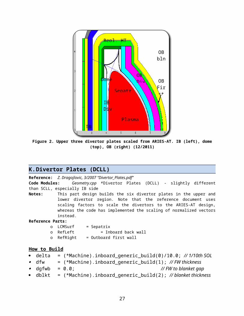
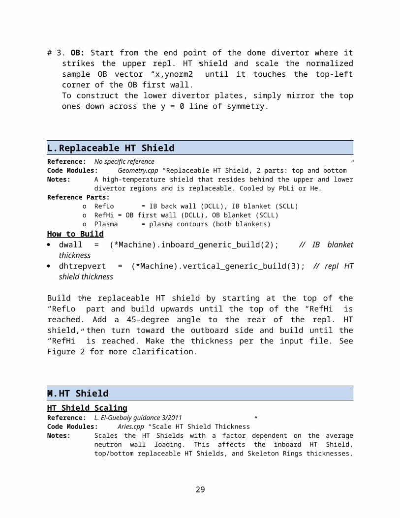
# 3. OB: Start from the end point of the dome divertor where it strikes the upper repl. HT shield and scale the normalized sample OB vector “x,ynorm2” until it touches the top-left corner of the OB first wall.To construct the lower divertor plates, simply mirror the top ones down across the y = 0 line of symmetry.

Figure 2. Upper three divertor plates scaled from ARIES-AT. IB (left), dome (top), OB (right) (12/2011)

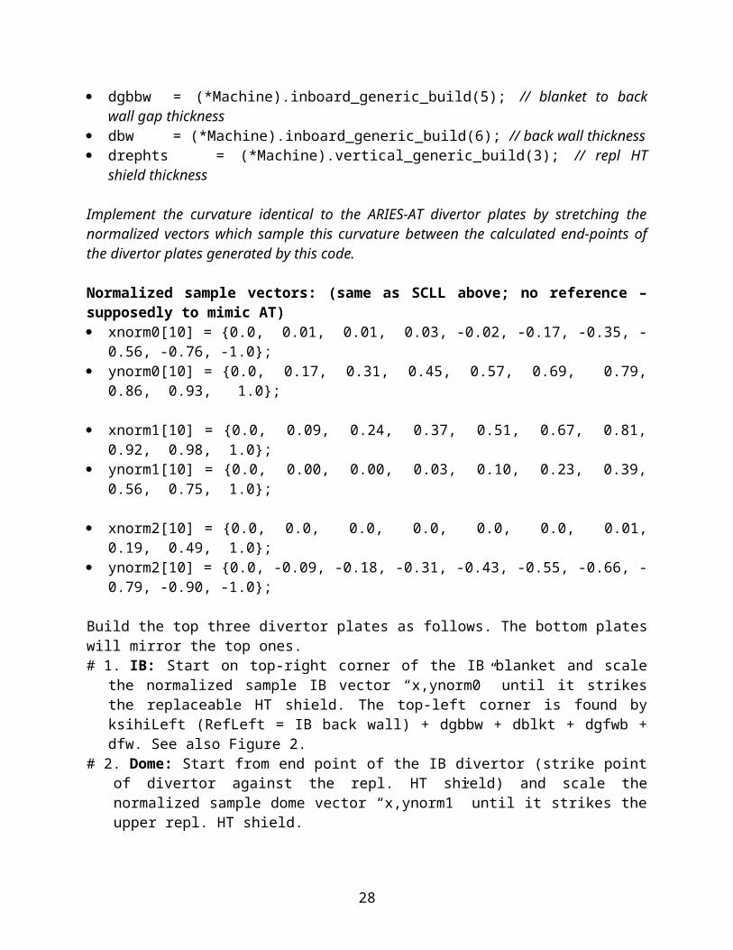
K. Divertor Plates (DCLL)Reference: Z. Dragojlovic, 3/2007 “Divertor_Plates.pdf”Code Modules: Geometry.cpp “Divertor Plates (DCLL) - slightly different than SCLL, especially IB side”Notes: This part design builds the six divertor plates in the upper and lower divertor region. Note that the

reference document uses scaling factors to scale the divertors to the ARIES-AT design, whereas the code has implemented the scaling of normalized vectors instead.

Reference Parts:o LCMSurf = Sepatrixo RefLeft = Inboard back wallo RefRight = Outboard first wall

How to Build delta = (*Machine).inboard_generic_build(0)/10.0; // 1/10th SOL dfw = (*Machine).inboard_generic_build(1); // FW thickness dgfwb = 0.0; // FW to blanket gap

Repl. HT shield

DomeOBDiv.

IB Div.

Sepatrix

PlasmaIB blnkt.

OBblnkt

.

OBFirst wall

19

dblkt = (*Machine).inboard_generic_build(2); // blanket thickness dgbbw = (*Machine).inboard_generic_build(5); // blanket to back wall gap thickness dbw = (*Machine).inboard_generic_build(6); // back wall thickness drephts = (*Machine).vertical_generic_build(3); // repl HT shield thickness

Implement the curvature identical to the ARIES-AT divertor plates by stretching the normalized vectors which sample this curvature between the calculated end-points of the divertor plates generated by this code.

Normalized sample vectors: (same as SCLL above; no reference – supposedly to mimic AT) xnorm0[10] = {0.0, 0.01, 0.01, 0.03, -0.02, -0.17, -0.35, -0.56, -0.76, -1.0}; ynorm0[10] = {0.0, 0.17, 0.31, 0.45, 0.57, 0.69, 0.79, 0.86, 0.93, 1.0};

xnorm1[10] = {0.0, 0.09, 0.24, 0.37, 0.51, 0.67, 0.81, 0.92, 0.98, 1.0}; ynorm1[10] = {0.0, 0.00, 0.00, 0.03, 0.10, 0.23, 0.39, 0.56, 0.75, 1.0};

xnorm2[10] = {0.0, 0.0, 0.0, 0.0, 0.0, 0.0, 0.01, 0.19, 0.49, 1.0}; ynorm2[10] = {0.0, -0.09, -0.18, -0.31, -0.43, -0.55, -0.66, -0.79, -0.90, -1.0};

Build the top three divertor plates as follows. The bottom plates will mirror the top ones.# 1. IB: Start on top-right corner of the IB blanket and scale the normalized sample IB vector

“x,ynorm0” until it strikes the replaceable HT shield. The top-left corner is found by ksihiLeft (RefLeft = IB back wall) + dgbbw + dblkt + dgfwb + dfw. See also Figure 2.

# 2. Dome: Start from end point of the IB divertor (strike point of divertor against the repl. HT shield) and scale the normalized sample dome vector “x,ynorm1” until it strikes the upper repl. HT shield.

# 3. OB: Start from the end point of the dome divertor where it strikes the upper repl. HT shield and scale the normalized sample OB vector “x,ynorm2” until it touches the top-left corner of the OB first wall.To construct the lower divertor plates, simply mirror the top ones down across the y = 0 line of symmetry.

L. Replaceable HT ShieldReference: No specific referenceCode Modules: Geometry.cpp “Replaceable HT Shield, 2 parts: top and bottom”Notes: A high-temperature shield that resides behind the upper and lower divertor regions and is

replaceable. Cooled by PbLi or He.Reference Parts:

o RefLo = IB back wall (DCLL), IB blanket (SCLL)o RefHi = OB first wall (DCLL), OB blanket (SCLL)o Plasma = plasma contours (both blankets)

How to Build dwall = (*Machine).inboard_generic_build(2); // IB blanket thickness dhtrepvert = (*Machine).vertical_generic_build(3); // repl HT shield thickness

20

Build the replaceable HT shield by starting at the top of the “RefLo” part and build upwards until the top of the “RefHi” is reached. Add a 45-degree angle to the rear of the repl. HT shield, then turn toward the outboard side and build until the “RefHi” is reached. Make the thickness per the input file. See Figure 2 for more clarification.

M.HT ShieldHT Shield ScalingReference: L. El-Guebaly guidance 3/2011Code Modules: Aries.cpp “Scale HT Shield Thickness”Notes: Scales the HT Shields with a factor dependent on the average neutron wall loading. This affects

the inboard HT Shield, top/bottom replaceable HT Shields, and Skeleton Rings thicknesses. Note: in C++ coding, "log" is actually the natural log (ln base e). "Log base 10 is "log10()"

DCLL blanket scaling factor = 7.5e-2*log(nwl/3.3); SCLL blanket scaling factor = 6.7e-2*log(nwl/3.3);

o nwl = average neutron wall loading, read from physics module

How to Build HT ShieldReference: Z. Dragojlovic, 3/2007 “HT_Shield.pdf”Code Modules: Geometry.cpp “HT Shield”Notes: - SCLL splits into IB and OB but builds it continuously. The HT shield resides behind the IB

blanket and behind the OB blanket II and wraps around the entire vessel.- DCLL maintains one continuous HT Shield only on IB side. The HT shield resides only behind the IB blanket and above/below the replaceable HT shield on the top/bottom of the vessel.

Reference Parts:SCLL reference parts for HT Shield:o RefLeft = BlanketInboardo RefDiag[2] = RepHTShield, [0] top, [1] bottomo RefTop = BlanketOutboardo RefRight = BlanketII

DCLL reference parts for HT Shield:o RefLeft = BackWallInboardo RefDiag[2] = RepHTShield, [0] top, [1] bottomo RefTop = BlanketOutboardo RefRight = BackWallOutboard

gapinb = (*Machine).inboard_generic_build(7); // IB blanket and HT shield gap dhtinb = (*Machine).inboard_generic_build(8); // IB HT shield thickness, scaled

down slightly in Aries.cpp dbwoutb = (*Machine).outboard_generic_build(8); // OB blanket II thickness dbwoutb = (*Machine).outboard_generic_build(9); // OB back wall II thickness (DCLL) gapoutb = (*Machine).outboard_generic_build(12); // OB blanket II to HT shield gap dhtoutb = (*Machine).outboard_generic_build(13); // OB HT shield thickness, scaled

down slightly in Aries.cpp dhtrepvert = (*Machine).vertical_generic_build(3); // repl HT shield thickness gapvert = (*Machine).vertical_generic_build(4); // repl HT shield and HT shield gap dhtvert = (*Machine).vertical_generic_build(5); // vertical HT shield thickness

Build the HT shield from contour lines by following the referenced parts (RefLeft, Diag, Top, Right) at the thickness specified in the generic_build.data input file. The HT shield generally hugs the IB blanket, the replaceable HT shield, and the OB blanket II or back wall. There is a 45-

21

degree notch at the top-left and top-right as the shield conforms to the replaceable HT shield on the inside and the vacuum vessel on the outside. The volume fractions of the different materials composing the part are specified in Cost.cpp

N. Skeleton Ring (DCLL)Reference: No specific referenceCode Modules: Geometry.cpp “Skeleton Ring (DCLL)”Notes: This assumes the HT shield (“HTShieldDCLL”) is in one piece. The skeleton ring is essentially

another shield for the DCLL design that wraps around the vessel behind the HT shield on the IB and vertical side and behind the OB back wall of the blanket.

Reference Part: DCLL HT shield

How to Build dhtinb = (*Machine).inboard_generic_build(8); // IB HT shield thickness gapinb = (*Machine).inboard_generic_build(9); // IB HT shield and SkelRing gap dvinb = (*Machine).inboard_generic_build(10); // IB SkelRing thickness dvoutb = (*Machine).outboard_generic_build(15); // OB SkelRing thickness drephtvert = (*Machine).vertical_generic_build(3); // vert repl HT shield thickness dhtvert = (*Machine).vertical_generic_build(5); // vert HT shield thickness gapvert = (*Machine).vertical_generic_build(6); // vert HT shield and SkelRing gap dvvert = (*Machine).vertical_generic_build(7); // vert SkelRing thickness

Build the skeleton ring by adding contour lines to follow the IB HT shield all the way around until the vertical. There is a notch in the top-left corner for the 45-degree angle in the HT shield. Then the skeleton ring follows the OB back wall as it continues around. The thickness of the ring is different for the IB/OB and the vertical dimensions.

O. Manifold (DCLL OB and vert)Reference: No specific referenceCode Modules: Geometry.cpp “Manifold (DCLL)”Notes: From L. El-Guebaly’s new (July 2011) design, contains PbLi+He. Some space is needed for

PbLi/He manifolds on the OB side just behind the OB and vertical skeleton ring on the DCLL blanket design. There are no manifolds on the IB side.

Reference Part: skeleton ring

How to BuildTBD

P. Manifolding (SCLL)Reference: New 2/2012 by L. Carlson, seen in ACT-SA (d)Code Version: ASC v.35Code Modules: Geometry.cpp “Manifolding (SCLL)”

22

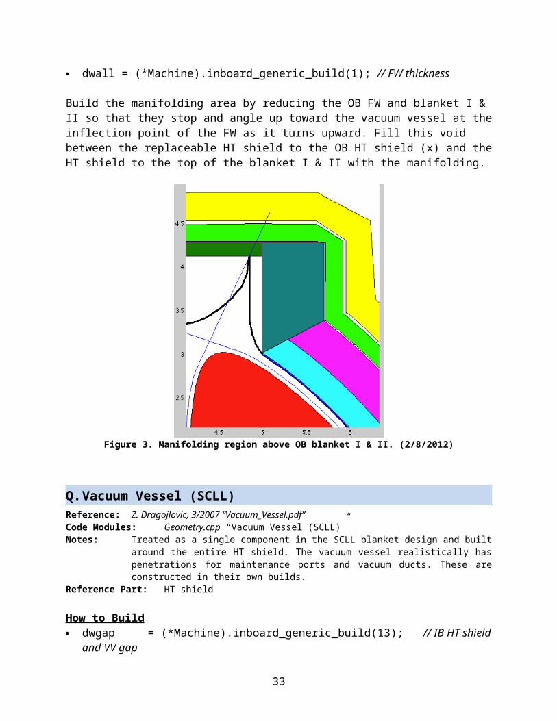
Notes: Requested by M. Tillack ~2/2012 to remove OB blanket FW, I & II extensions on the top and bottom and to add a manifolding region in preparation for future detailed design work in this area. This region is to the right of OB divertors and above/below OB blankets and will be used to combine and route He & PbLi into and out of the blankets/vessel. It will be composed of ~30% FS, ~50% PbLi, ~10% He and ~10% SiC-comp.

Reference Part: Replaceable HT shield [0], FW, blanket I, blanket II

How to Build dwall = (*Machine).inboard_generic_build(1); // FW thickness

Build the manifolding area by reducing the OB FW and blanket I & II so that they stop and angle up toward the vacuum vessel at the inflection point of the FW as it turns upward. Fill this void between the replaceable HT shield to the OB HT shield (x) and the HT shield to the top of the blanket I & II with the manifolding.

Figure 3. Manifolding region above OB blanket I & II. (2/8/2012)

Q. Vacuum Vessel (SCLL)Reference: Z. Dragojlovic, 3/2007 “Vacuum_Vessel.pdf”Code Modules: Geometry.cpp “Vacuum Vessel (SCLL)”Notes: Treated as a single component in the SCLL blanket design and built around the entire HT shield.

The vacuum vessel realistically has penetrations for maintenance ports and vacuum ducts. These are constructed in their own builds.

Reference Part: HT shield

How to Build

23

dwgap = (*Machine).inboard_generic_build(13); // IB HT shield and VV gap dwall = (*Machine).inboard_generic_build(14); // IB VV thickness ibvv = (*Machine).inboard_generic_build(14); // IB VV thickness obvvgap = (*Machine).outboard_generic_build(18); // OB HT shield and VV gap obvv = (*Machine).outboard_generic_build(19); // OB VV thickness

Build the vacuum vessel by following the HT shield all the way around. Mimic the top-left and top-right corners, which are notched. The IB/vertical builds are of different thickness than the OB build, as specified in the generic build input file. See Figure 1 for more details.

R. Vacuum Vessel (DCLL)Reference: Z. Dragojlovic, 3/2007 “Vacuum_Vessel.pdf” No specific documentation as to why there are 4

components of the DCLL vacuum vessel.Code Modules: Geometry.cpp “1/4, 2/4, 3/4, 4/4 Vacuum Vessel (DCLL)”Notes: Treated as four separate components in the DCLL blanket design and built around the entire

skeleton ring. The vacuum vessel realistically has penetrations for maintenance ports and vacuum ducts. These are constructed in their own builds.

Reference Part: skeleton ring

How to Build VV 1 of 4 Inboard gapinb = (*Machine).inboard_generic_build(13); // IB skel ring and VV gap dringvert = (*Machine).vertical_generic_build(7); // vert skel ring thickness dvinb = (*Machine).inboard_generic_build(14); // IB VV thickness

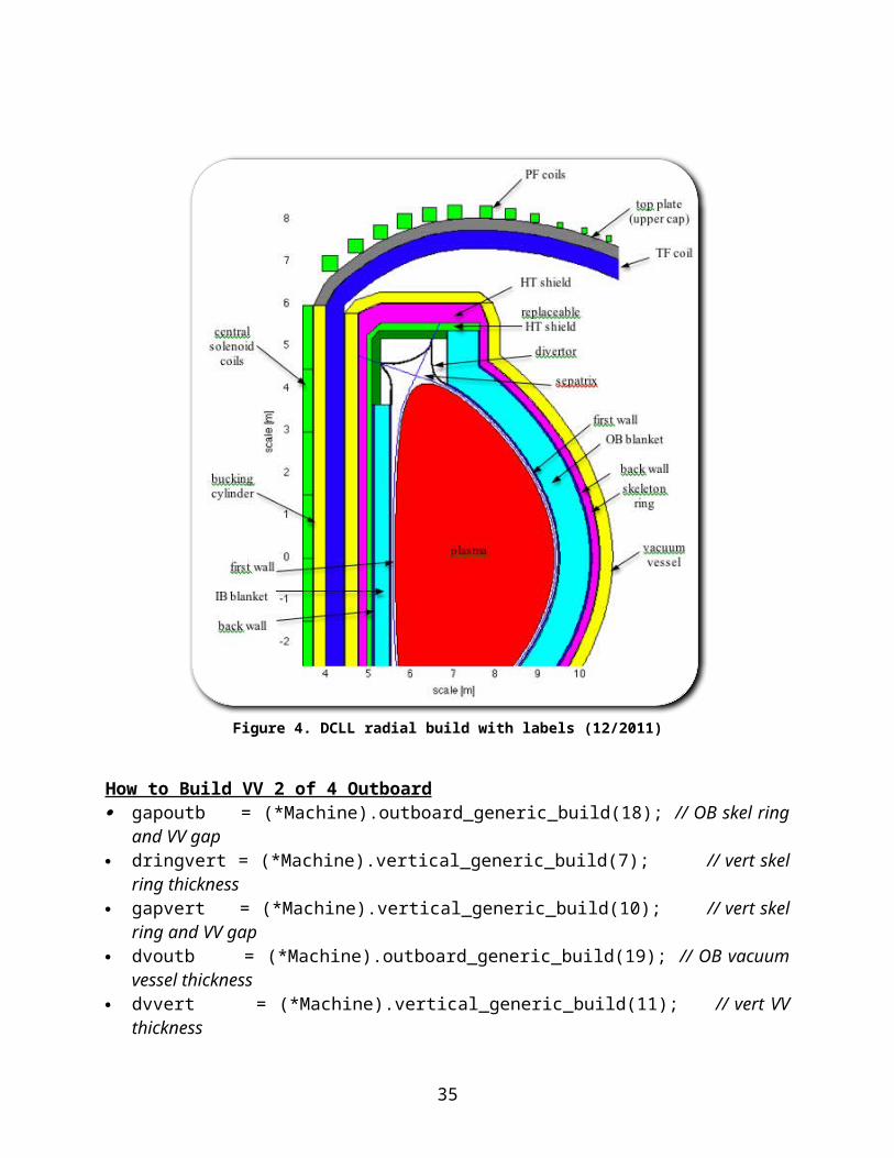
Build the inboard portion of the vacuum vessel by adhering to the IB skeleton ring. Follow the ring all the way to the top until the bottom notch of the ring. See Figure 4 for more details. The thickness of the IB VV is specified in the radial build input file as well as any gaps.

24

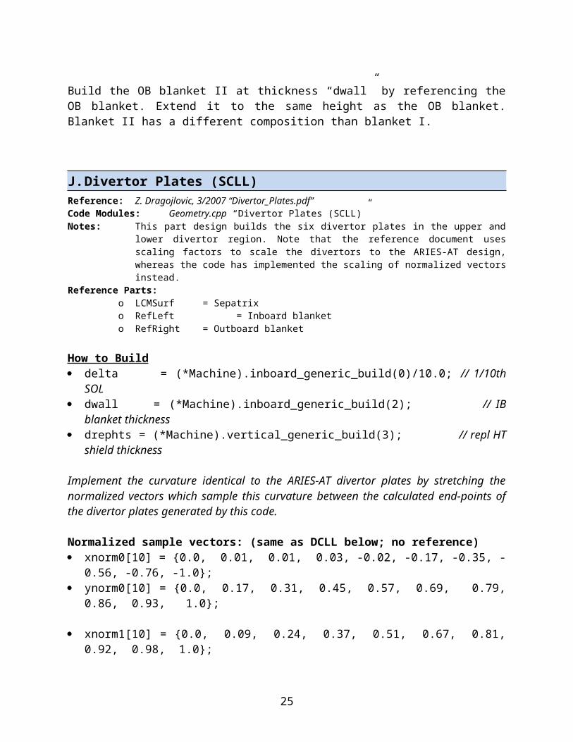
Figure 4. DCLL radial build with labels (12/2011)

How to Build VV 2 of 4 Outboard gapoutb = (*Machine).outboard_generic_build(18); // OB skel ring and VV gap dringvert = (*Machine).vertical_generic_build(7); // vert skel ring thickness gapvert = (*Machine).vertical_generic_build(10); // vert skel ring and VV gap dvoutb = (*Machine).outboard_generic_build(19); // OB vacuum vessel thickness dvvert = (*Machine).vertical_generic_build(11); // vert VV thickness

Build the outboard portion of the vacuum vessel by adhering to the OB skeleton ring. Follow the ring all the way to the top until the top notch of the ring. This will allow the OB VV to be removed for maintenance. See Figure 4 for more details. The thickness of the OB VV is specified in the radial build input file as well as any gaps.

How to Build VV 3 of 4 Bottom, by symmetryBuild the bottom vacuum vessel by simply mirroring the top by symmetry.

How to Build VV 4 of 4 Top

25

dhtinb = (*Machine).inboard_generic_build(8); // IB HT shield thickness dringinb = (*Machine).inboard_generic_build(10); // IB skel ring thickness gapinb = (*Machine).inboard_generic_build(13); // IB skel ring and VV gap dringvert = (*Machine).vertical_generic_build(7); // vert skel ring thickness gapvert = (*Machine).vertical_generic_build(10); // vert skel ring and VV gap dvinb = (*Machine).inboard_generic_build(14); // IB VV thickness dvoutb = (*Machine).outboard_generic_build(19); // OB vacuum vessel thickness dhtrepvert = (*Machine).vertical_generic_build(3); // vert repl HT shield thickness dsrvert = (*Machine).vertical_generic_build(7); // vert skel ring thickness dvvert = (*Machine).vertical_generic_build(11); // vert VV thickness

Build the top portion of the vacuum vessel by adhering to the top of the skeleton ring. Follow the ring from the top of the IB VV to the top of the OB VV. The vacuum vessel components should fit together cleanly. See Figure 4 for more details. The thickness of the top VV is specified in the radial build input file as well as any gaps.

S. TF MagnetReference: Z. Dragojlovic, L. Bromberg, 5/2007 “TF_Magnet.pdf” and

Z. Dragojlovic, 8/2010 “HowToBuildTFCoil.pdf”Code Modules: Geometry.cpp “TF Magnet: r-theta plane, ‘Next Step’, conservative costing”Notes: The seven TF coil designs are all similar to each other. The design in use currently is the third (iii)

one below. The other algorithms won’t be detailed in this document.a. r-theta plane

i. PPPL Version, conservative Costingii. PPPL Version

iii. Next Step, conservative costing (currently in use)iv. Next Stepv. HTS

vi. Nb3Snvii. ARIES-AT coil design with fixed volume fractions

b. r-z plane – revolvedReference Part: plasma and vacuum vessel

How to Build: TF Coil, r-theta plane – “Next Step, conservative costing” const pi = 4.0*atan(1.0); const muo = 4.0*pi*1.0e-7; sigma_sheath = maximum stress in protective sheath around strands (defined from

magnets.data input file) sigmab = maximum allowed stress in the coil casing (defined from magnets.data input file) ksiloP = (*Plasma).bounding_box(0, "outer"); // Define the bounding box for the plasma ksihiP = (*Plasma).bounding_box(2, "outer"); // Define the bounding box for the plasma ksihiVV = (*VVRefBody)[1].bounding_box(2, "outer"); // Define the bounding box for VV ksiloVV = (*VVRefBody)[0].bounding_box(0, "outer"); // Define the bounding box for VV gapvvtf = (*Machine).inboard_generic_build(17); // VV and IB TF coil gap rTFinner = ksiloVV - gapvvtf; // radius of inner TF coil

26

Maximum Magnetic Field:o Ro = (*Machine).plasma_major_radius();o Btmax = Bt*Ro/rTFinner;

(*Machine).get_maximum_magnetic_field_at_tf_coil(Btmax); // puts BTmax into this fcn

Current Density in Superconductor versus Btmax function for Nb3Sn @ 4.2 Ko btmaxVec[5] = {6.0, 10.0, 14.0, 16.0, 18.0};o jscVec[5] = {1.52e9, 1.35e9, 8.84e8, 5.43e8, 1.30e8};

[Super-conducting current table from “TF_Magnet.pdf” The code interpolates to the nearest value in the table.]

Super-conducting current polynomial based on the table values (this SUPERCEEDS the table above.) [C. Kessel also uses this in his code "sysengr.f" line ~364]o Jsc = -9.1226*pow(Btmax,2)*1.0e6 + 1.0301*Btmax*1.0e8 + 1.2308*1.0e9;

Cross section of the winding pack:o Jcu = Current density in copper from magnets.data input fileo f_he = Volume fraction of He coolanto dsheath = pow(Btmax,2)/(2.0*muo*sigma_sheath); // Sheath thicknesso f_sheath = 1.0 - pow(1.0 - dsheath, 2); // Sheath fractiono f_ins = Volume fraction of the insulatoro Itf = Nominal current in TF coil

Cross-sectional areas:o Acu = Itf/Jcu;o Asc = Itf/Jsc;o Astrands = Acu + Asc;o Aturn = Astrands/(1.0 - f_he - f_sheath - f_ins); // C.K. sysengr.f line ~376

Cross-sectional area of a single turn in a winding packo Ains = Aturn*f_ins;o Asheath = Aturn*f_sheath;

Coil Casing Cross Sectiono Ntf = Number of TF coilso b = Side thickness of the coil casing is b/2o ATF = Aturn*Bt*2.0*pi*Ro/(Ntf*Itf*muo); // Area of a TF coil single winding packo Nwp = int(ATF/Aturn); // Number of turns per winding pack (WP)o (*Machine).get_number_of_tf_cable_turns(Nwp); // puts Nwp into this function

Coil Casing Thickness Loopo a = b; // b = side thickness of coil casing, initial guess for casing thicknesseso for(int j=0; j<5; j++) { // START LOOPo R1 = rTFinner - 2.0*a; // Calculate R1, the inner radius of inner TF coil lego for(int i=0; i<5; i++) { o R1 = rTFinner - a - ATF/( 2.0*pi*R1/Ntf - b); } // similar to CK sysengr.f ~382

27

o wTF = 2.0*pi*R1/Ntf - b; // width of the TF coilo dTF = ATF/wTF; // winding pack (conductors) thickness if lumped all together

o Calculate R2 based on the clearance on the outboard side of the TF coils needed for removal of the power core module for maintenance purpose

o cTFVV = Clearance between the Vacuum Vessel and the TF coil outmost edgeo R2 = ksihiVV + R1 + cTFVV/sin(pi/Ntf); // inner radius of outer TF coil leg

Structure calculation based on bending:o G1 = pow(3.0/(16.0*sigmab*muo), 0.5);o G2 = Bt*Ro/(R2-R1);o G3 = pow((R2*R2-R1*R1)*(1+log(R2/R1)) +

R1*R2*(2-(log(R2/R1))*(log(R2/R1))),0.5 ); // note extra log is for log^2, reference?

o coeff = 0.208; // OK for ACT-I, II. Coefficient is a casing thickness multiplier based on scaling FEA results to match AT casing.

o a = coeff*G1*G2*G3; o // “a” is the total coil casing, so a/2 + winding pack + a/2 = total TF thickness. This

thickness includes coil case and/or all internal structure. There is a tradeoff between internal and coil casing structure – if one goes down, the other must go up.

o } // END LOOP

Defining parameters of the coil cross section (the thickness is uniform along the TF coil perimeter for now) delta_inner = a + dTF; // total thickness of inner leg equal to casing + magnet delta_outer = a + dTF; // total thickness of outer leg equal to casing + magnet delta_top = a + dTF; // total thickness of top/bottom part equal to casing + magnet

o R2 = R2 + delta_outer; // Update the outer radius of the outer surface of the TF coil:o (*Machine).get_tf_coil_radii(R1, R2); // Get the inner-most and outer-most radius of

the TF Coilo delta = max(delta_inner, max(delta_outer, delta_top));o width = wTF + b; // width of TF coil

Cross sectional area of the composition: Acomp = delta*width; // cross sectional area of the composition Astructure = delta*width - dTF*wTF; // steel (should be ~75% of WP+CC) vfrac_structure = Astructure/Acomp; // volume fraction of SS316 structure vfrac_sc = Asc*Nwp/Acomp; // superconductor (Nb3Sn) vfrac_cu = Acu*Nwp/Acomp; // copper (Cu) vfrac_sheath = Asheath*Nwp/Acomp; // sheath (Inconel) vfrac_ins = Ains*Nwp/Acomp; // insulator (Polyamide) vfrac_he = 1.0 - vfrac_structure - vfrac_sc - vfrac_cu - vfrac_sheath - vfrac_ins;

// He coolant

28

Get TF Cross-Section Material Components:o Gets the material costs, mass, etc from Part.cpp based on (1) material name, (2) volume

fraction, (3) density fraction, and (4) the cost base. (*Magnet).get_cross_section(0, delta, width); (*Magnet).get_material_component("SS316", vfrac_structure, 1.0, 0); (*Magnet).get_material_component("Nb3Sn", vfrac_sc, 1.0, 1); (*Magnet).get_material_component("Cu", vfrac_cu,1.0, 2); (*Magnet).get_material_component("Inconel", vfrac_sheath, 1.0, 3); (*Magnet).get_material_component("Polyamide", vfrac_ins, 1.0, 4); (*Magnet).get_material_component("He", vfrac_he, 1.0, 5);

How to Build: TF Coil, r-z plane – “revolved” This part design builds the TF coils by revolving their cross-sections in the r-z plane to create the coil’s shape about the “Princeton-D” ellipse. dw = (*Magnet).cross_section_width(0); // TF magnet wall thickness hxp = (*Machine).xpoint(1); // X-point height R1 = (*Machine).tf_magnet_inner_leg_radius(); // TF Coil inboard radii R2 = (*Machine).tf_magnet_outer_leg_radius(); // TF Coil outboard radii r1 = R1 + dw; r2 = R2 - dw; Ro = (*Machine).plasma_major_radius(); // Plasma major radius ao = (*Machine).plasma_minor_radius(); // Plasma minor radius

Define the parameters of the “Princeton-D” ellipse [1]:[1] Richard J. Thome, John M. Tarrh, “MHD and Fusion Magnets – Field and Force Design Concepts”, John Wiley & Sons, 1982. b = etahi + 1.043 ; // radius on the vertical axis, same as cap below, reference? a1 = (Ro-r1)/pow(1.0-pow( 0.95*etahi/b, 2.0 ), 0.5 ); a2 = r2 - Ro;

Build the TF coil by following the contour of the inboard vacuum vessel at the computed thickness. Once the top of the VV is cleared, the contour of the Princeton-D ellipse can be formed.

TF coil contour loop int len = 300; // Transform the plasma into the TF coil contour double *x, *y; x = new double [len]; y = new double [len]; x[0] = r1; y[0] = 0.0; double delx = 2*(r2-r1)/(len-3); for(int i=1; i<len-1; i++) // loop over TF coil contour { if(i < (len+1)/2 ) // upper half of the coil

{ int c;

29

if(i == 1){c=0;} else {c=1;} x[i]=x[i-1]+c*delx; if(x[i] < (r2-a2)) // inner ellipse { y[i] = b*pow(1.0-pow((x[i]-Ro)/a1, 2.0), 0.5); } else // outer ellipse { y[i] = b*pow(1.0-pow((x[i]-Ro)/a2, 2.0), 0.5); } } else // lower half of the coil { if(i == (len+1)/2) { x[i] = r2; } else { x[i] = x[len-i]; } if(i == len-2) x[i] = x[0]; if(x[i] < (r2-a2)) // inner ellipse { y[i] = -b*pow(1.0-pow((x[i]-Ro)/a1, 2.0), 0.5); } else // outer ellipse { y[i] = -b*pow(1.0-pow((x[i]-Ro)/a2, 2.0), 0.5); } } } // end loop over TF coil contour

T. Bucking CylinderReference: No specific documentation.Code Modules: Geometry.cpp “Bucking Cylinder”Notes: This resides just around the central solenoid and gives it strength and support. Its thickness

depends on the yield stress of the casing as well as the maximum toroidal field BTmax.Reference Part: TF coil and vacuum vessel

How to Build sigmaYield = casing yield stress for the coil case from magnets.data input file sigma = 2.0/3.0*sigmaYield; Btmax = Bt*(*Machine).plasma_major_radius()/ksilo; dscr = (*Machine).inboard_generic_build(21); // TF coil to bucking cyl gap dwall = pow(Btmax,2)*ksilo/(2.0*muo*sigma); // bucking cyl thickness

Build the bucking cylinder at the computed thickness by referencing the inboard portion of the TF coil and following it up until the top of the vacuum vessel.

U. Upper Toroidal Cap on the TF CoilReference: No specific documentation.Code Modules: Geometry.cpp “Upper Toroidal Cap on the TF Coil”Notes: This cap supports the PF coils that lie on top of the TF coils on the top of the machine. Its

thickness depends on the yield stress of the casing and BTmax.Reference Part: TF coil and vacuum vessel

30

How to Build sigmaYield = casing yield stress for the coil case from magnets.data input file sigma = 2.0/3.0*sigmaYield; Btmax = Bt*(*Machine).plasma_major_radius()/ksilo; dwgap = (*Machine).vertical_generic_build(18); // TF coil to toroidal cap gap dwall = pow(Btmax,2)*ksilo/(2.0*muo*sigma); // toroidal cap thickness dmagnet = (*RefBody).cross_section_width(0); // TF magnet thickness

Ro = (*Machine).plasma_major_radius(); R1 = (*Machine).tf_magnet_inner_leg_radius(); R2 = (*Machine).tf_magnet_outer_leg_radius(); r1 = R1 + dmagnet; r2 = R2 - dmagnet; b = etahiV + 1.043; // TF ellipse radius on the vertical axis a2 = r2 - Ro; // TF outer ellipse radius on the horizontal axis

Limiting point on the outer TF coil contour - this point is determined by the height of the vacuum vessel etahiV y_tf = etahiV; x_tf = Ro + a2*sqrt(1.0 - pow(y_tf/b,2.0)); g = (x_tf - Ro)/a2; alpha_t = atan( -b/a2*g/sqrt(1.0 - pow(g,2.0)) ); alpha_n = alpha_t + pi/2.0;

Build the upper toroidal cap at the computed thickness by starting at the top of the bucking cylinder and following the contour of the TF coil. End the cap when no more PF coils need support and before the top-most portion of the vacuum vessel is reached (cannot block maintenance door access).

V. Lower Toroidal Cap on the TF CoilReference: No specific documentation.Code Modules: Geometry.cpp “Lower Toroidal Cap on the TF Coil – By Design OR By Symmetry”Notes: This cap supports the PF coils that lie below the TF coils on the bottom of the machine. Its

thickness depends on the yield stress of the casing and BTmax.Reference Part: TF coil and vacuum vessel

How to Build sigmaYield = casing yield stress for the coil case from magnets.data input file sigma = 2.0/3.0*sigmaYield; Btmax = Bt*(*Machine).plasma_major_radius()/ksilo; dwgap = (*Machine).vertical_generic_build(18); // TF coil to upper cap gap dwall = pow(Btmax,2)*ksilo/(2.0*muo*sigma); // toroidal cap thickness dmagnet = (*RefBody).cross_section_width(0); // TF magnet thickness Ro = (*Machine).plasma_major_radius(); R1 = (*Machine).tf_magnet_inner_leg_radius();

31

R2 = (*Machine).tf_magnet_outer_leg_radius(); r1 = R1 + dmagnet; r2 = R2 - dmagnet; b = -etaloV + 1.043; // TF ellipse radius on the vertical axis a2 = r2 - Ro; // TF outer ellipse radius on the horizontal axis

Limiting point on the outer TF coil contour - this point is determined by the height of the vacuum vessel etahiV y_tf = etaloV; x_tf = Ro + a2*sqrt(1.0 - pow(y_tf/b,2.0)); g = (x_tf - Ro)/a2; alpha_t = atan( b/a2*g/sqrt(1.0 - pow(g,2.0)) ); alpha_n = alpha_t - pi/2.0;

Build the lower toroidal cap at the computed thickness by starting at the bottom of the bucking cylinder and following the contour of the TF coil. End the cap when no more PF coils need support and before the bottom-most portion of the vacuum vessel is reached (cannot block maintenance door access). Alternatively, the upper TF coil cap can be mirrored to the bottom by symmetry.

W.PF Coil DesignReference: Z. Dragojlovic, C. Kessel, 10/2007 “PF_Magnet.pdf”Code Modules: Geometry.cpp “PF Coil Design”Notes: The PF coils run in the poloidal direction and lie on top of and bottom of the TF coil caps. PF coils

#0-3 from top + #32-35 from bottom create the central solenoid; #4-17 lie along the top and #18-31 lie along the bottom (going clock-wise); #4-17 are duplicated as spares. See Figure 7 for an enumeration of the PF coils and their locations.

Reference Part: bucking cylinder, top and bottom TF coil caps

How to Build Coil currents at zero flux state:

o ccoil1[18] = {1.24, 0.47, 1.85, 7.08, 4.29, 4.05, 3.87, 4.20, 4.02, 3.64, 3.02, 2.27, 1.35, 0.15, -1.35, -3.11, -4.99, -6.83};

o ccoil2[18] = {1.03, 1.76, 3.23, 5.85, 3.76, 3.78, 3.81, 4.36, 4.37, 4.14, 3.59, 2.86, 1.91, 0.57, -1.17, -3.32, -5.74, -8.15};

Rate of change of coil current with flux state: o dcdp[18] = {1.40, 0.47, 0.54, 2.44, 0.87, 0.67, 0.52, 0.49, 0.31, 0.19, 0.10, 0.02, -0.03,

-0.07, -0.06, 0.02, 0.14, 0.29};

Current limiters:o qmax = upper limiter of the currento qmin = lower limiter of the current

Determine PF coil currents at given q95 and scale to plasma current:

32

o qmhd = (*Machine).plasma_edge_safety_factor();o aip = (*Machine).plasma_current();o for(int i=0; i<18; i++) // 0-17 are all PF coils above midplane

{ if(qmhd >= qmax) { ccoil[i] = ccoil2[i]*(aip/12.8); } if(qmhd <= qmin) { ccoil[i] = ccoil1[i]*(aip/12.8); } if(qmhd > qmin && qmhd < qmax) { ccoil[i] = ccoil1[i] + ((ccoil2[i]-ccoil1[i])/(qmax-qmin))*(qmax-qmhd); ccoil[i] = ccoil[i]*(aip/12.8); } }

Calculate flux swing required to rampup to Ip:o r = (*Machine).plasma_major_radius();o asp = (*Machine).plasma_major_radius() / (*Machine).plasma_minor_radius(); // plasma

aspect ratio o ak = (*Machine).plasma_elongation(); // plasma elongationo betap = (*Machine).plasma_poloidal_beta();o e = 1.0/asp;o ali = 0.50;o ce = 0.6;

o a1 = (1.0 + 1.81*pow(e, 0.5) + 2.05*e)*log(8.0/e)-(2.0 + 9.25*pow(e, 0.5) - 1.21*e);o a2 = 0.73*pow(e, 0.5)*(1.0 + 2.0*pow(e, 4.0) - 6.0*pow(e, 5.0) + 3.7*pow(e, 6.0));o a3 = 1.0 + 0.98*pow(e, 2.0) + 0.49*pow(e, 4.0) + 1.47*pow(e, 6.0);o a4 = 0.25*e*(1.0 + 0.84*e - 1.44*pow(e, 2.0));

o als = a1*(1.0 - e)/(1.0 - e + a2*ak);o am = pow(1.0 - e, 2.0)/(pow(1.0 - e, 2.0)*a3 + a4*pow(ak, 0.5));o alext = als - (am/4.0)*(log(8.0/(e*pow(ak, 0.5))) + betap + ali/2.0 - 3.0/2.0);o alext2 = als;o dfcsx = 1.2566*aip*r*(alext + (ali/2.0) + ce);o dfcsx2 = 1.2566*aip*r*(alext2 + (ali/2.0) + ce);

Calculate forward and back bias coil currents:o for(int i=0; i<18; i++)o { ccoilf[i] = ccoil[i] - (dcdp[i]*dfcsx2/2.0)/25.0;o ccoilb[i] = ccoil[i]/4.0 + (dcdp[i]*dfcsx2/2.0)/25.0; }

Determine maximum current in each PF coil:o ccoilmx[18];o for(int i=0; i<18; i++)o { ccoilmx[i] = max( max(ccoilb[i], ccoilf[i]), ccoil[i] ); }

33

Calculate coil thickness based on jSC central solenoid (first 4 coils in array) outer radius of the central solenoid calculated as inner radius of the bucking cylinder minus the gap between central solenoid and bucking cylindero csbcgap = (*Machine).inboard_generic_build(23); // central solenoid to buck cyl gapo rpfout = ksiloBC - csbcgap; o Bmaxlimpf = Maximum allowed field on PF coilso ccoilcsmx = max( max(ccoilmx[1], ccoilmx[2]), max(ccoilmx[3], ccoilmx[4]) );o ccoilcsmx = fabs(ccoilcsmx);o bmaxpf = dfcsx/(2.0*pi*pow(rpfout, 2.0));o if(bmaxpf > bmaxlimpf)o { cout << "bmaxpf = " << bmaxpf << " which is greater than the limit" << bmaxlimpf

<< "\n"; (*Machine).get_data_point_filter(3, 3); return; }

Maximum allowed current density in superconductor = xjsclimpf; o if(bmaxpf > 12.0)o { xjsclimpf = -2.1e8*bmaxpf + 3.78e9; } o elseo { xjsclimpf = -4.0e7*bmaxpf + 1.74e9; }o hcs = 2.0*etahiBC; // bucking cylinder height

Areas: o Asc = ccoilcsmx*1.0e6/xjsclimpf; // total area of the superconductoro sigma_sheath = maximum stress in protective sheath around strandso Asheath = ccoilcsmx*1.0e6*bmaxpf*rpfout/sigma_sheath; // total area of sheatho J2_tau = quench protection parametero tau = quench timeo Acu = ccoilcsmx*1.0e6/pow(2.0*J2_tau/tau,0.5); // total area of the Cuo f_He = volume fraction of He coolanto Ahe = (Asc+Acu)*f_He; // total area of the coolant (He)o Astructure = ccoilcsmx*1.0e6*bmaxpf*rpfout/sigma; // total area of the stainless steel

structureo f_ins = volume fraction of the insulatoro Ains = (Asc + Asheath + Acu + Ahe + Astructure)*f_ins/(1.0 - f_ins); o Atotal = Asc + Acu + Asheath + Astructure + Ahe + Ains; // total area of the insulator

Area fractionso fstarea = (Asheath+Astructure)/Atotal;o fcuarea = Acu/Atotal;o fcoolarea = Ahe/Atotal;o finsarea = Ains/Atotal;o fscarea = 1.0 - fstarea - fcuarea - fcoolarea - finsarea;o dr = 8.0*ccoilcsmx*1.0e6/(hcs*fscarea*xjsclimpf);o rpfin = rpfout - dr;

34

Locations of the PF coils Build the central solenoid by following the inside of the bucking cylinder up to its same height. The central solenoid is composed of 8 coils, #0-3 and #32-35. All the PF coils on the top and bottom toroidal cap are equally spaced. Realistically though, the PF coils will need to be shifted either up or down to make room for the vacuum vessel duct penetration. If the slope of the cap surface is going up, they are on the left side of the spacer. If the slope is going down, they are on the right side. The spacer rpf[i] is placed by dividing the width of the toroidal cap by 14, which is the number of coils on the top. Starting from the 12th coil, the spacer is shifted to the left by dx[i]. Mirror the top coils down to the bottom cap by symmetry.

rpf[i] = ksiloT + spacing*(i-3); if( i > 9 ) rpf[i] = rpf[i] - dx[i]/2.0;

double dist = 1.0e6; int ipfc;

for(int j=0; j<lttc; j++) { double xttc = (*TopTCap).contour(j, 0, "outer"); double yttc = (*TopTCap).contour(j, 1, "outer"); if( dist > fabs(xttc-rpf[i]) && xttc < (*TopTCap).contour(j+1, 0, "outer") ) { dist = fabs(xttc-rpf[i]); ipfc = j; if ( yttc >= (*TopTCap).contour(j-1, 1, "outer") ) { position[i] = "left"; } else { position[i] = "right"; } } } zpf[i] = (*TopTCap).contour(ipfc, 1, "outer"); } } END

X. Cryogenic DomeReference: Z. Dragojlovic, 3/2007 “Cryogenic_Dome.pdf”Code Modules: Geometry.cpp “Cryogenic Dome”Notes: The cryogenic dome is created around the entire tokamak using the TF coil as its reference. It is

also sometimes called the "cryodome or cryostat."Reference Part: TF coil

How to BuildInner Contour: outer contour is the inner + the cryodome thickness ksilo = (*RefBody).bounding_box(0, "outer"); // min IB TF coil (x) etalo = (*RefBody).bounding_box(1, "outer"); // bottom TF coil (y) ksihi = (*RefBody).bounding_box(2, "outer"); // max OB TF coil (x) etahi = (*RefBody).bounding_box(3, "outer"); // top of TF coil (y) dwall = (*Machine).vertical_generic_build(21); // cryodome thickness

xs[0] = 0.0; ys[0] = 1.5*etahi;

35

xs[20] = ksilo + ( ksihi - ksilo )*1.1; ys[20] = etahi*1.1;

for(int i=1; i<20; i++) { xs[i] = xs[0] + i*xs[20]/20; ys[i] = ys[20] + (ys[0] - ys[20])*2.0/pi*atan(2.0*fabs( xs[20] - xs[i])); }

xs[21] = xs[20]; ys[21] = 1.5*etalo; xs[22] = 0.001; ys[22] = ys[21]; xs[23] = 0.0; ys[23] = ys[21];

Build the cryodome by following the contour lines and reference points as indicated above. Then, build the outer contour at the thickness given by the vertical build input file.

Y. Maintenance Port WindowReference: No specific documentation.Code Modules: Geometry.cpp “Maintenance Port Window in-between the TF Coils”Notes: A maintenance port window resides in each sector between TF coils and allows access to the OB

vacuum vessel door for removal and maintenance of the power core components. Reference Part: TF coil and vacuum vessel

How to BuildThe maintenance port window is simply the area enclosed by the width between the TF coils and the height of the outboard vacuum vessel. See also Maintenance Ports build.

Z. Maintenance PortsReference: No specific documentation.Code Modules: Geometry.cpp “Maintenance Ports”Notes: The maintenance ports are the areas in each sector between TF coils. The ports allow access to the

OB vacuum vessel door for removal and maintenance of the power core components. Reference Part: vacuum vessel and cryodome

How to Build ductwall = (*Machine).vertical_generic_build(11)/4.0; // 1/4th VV thickness

Volume and Surface Areas (*MPort).get_volume(); // volume of one side wall of the maintenance port vSideWall = (*MPort).volume();

Volume of the top and bottom walls of the maintenance port

36

rTop = (*MPort).bounding_box(0, "outer"); lTop = ksihi - rTop; vTopWall = 2.0*rTop*sin(pi/16.0)*lTop*ductwall;

Volume of the outer door of the maintenance port etaMPhi = (*MPort).bounding_box(3, "outer"); etaMPlo = (*MPort).bounding_box(1, "outer"); vOuterDoor = 2.0*rTop*sin(pi/16.0)*(etaMPhi-etaMPlo)*ductwall;

Amount of volume to add to already included side wall: vPlus = 2.0*vTopWall + vSideWall + vOuterDoor; (*MPort).add_to_volume(vPlus);

Build the maintenance port by coming directly off the top and bottom of the vacuum vessel components and extending out radially until the cryodome is reached. The width of the port is the distance between the TF coils specified at the radius of the outboard vacuum vessel. The volume of the maintenance port is quite substantial – see Figure 5 for a sense of scale. The volume includes all the space enclosed within the pie-shaped bounding box of the OB VV door to the cryodome at a height of the entire vacuum vessel.

Figure 5. SCLL radial build showing maintenance port extending radially from OB VV out in-between the TF coil, then through the cryodome. (12/2011)

AA. Upper Vacuum Vessel DuctReference: No specific documentation.Code Modules: Geometry.cpp “Upper Vacuum Vessel Duct – Bottom, Top and Side Wall”Notes: The vacuum ducts provide a way to access the inside of the vacuum vessel for pumping. The

vacuum ducts penetrate the vacuum vessel, route in-between the TF coils, penetrate the upper

37

toroidal cap, nudge the PF coils slightly so there is room to come between them and penetrate the cryostat for connection to vacuum pumps outside the tokamak. See Figure 6 for a visualization.

Reference Part: vacuum vessel, TF coil and cryodome

How to Build – Bottom WallThis design function builds the bottom wall of the upper vacuum duct. etahiVV = (*Vessel)[0].bounding_box(3, "outer"); // top of vert VV (y) ksihiVV = (*Vessel)[0].bounding_box(2, "outer"); // OB VV (x) ksiloVV = (*Vessel)[0].bounding_box(0, "outer"); // IB VV (x) ksimedVV = 0.4*(ksiloVV + ksihiVV); // middle of VV

ksihiCryo = (*Cryo).bounding_box(2, "outer"); // Relevant bounding box coordinates of the outer cylindrical surface of the cryostat

etahiMagnet = (*Magnet).bounding_box(3, "inner"); // Ordinate of the highest point of the inner surface of the TF magnet

hVVTF = etahiMagnet - etahiVV; // Largest vert gap between vacuum vessel and TF coil ductwidth = 0.15*(ksihiVV - ksiloVV); // Width of the duct in the vertical plane ductwall = (*Machine).vertical_generic_build(11)/4.0; // Duct wall thickness = 1/4th VV

thickness

Build the bottom wall by referencing the top of the vertical VV at the location “ksimedVV+ductwidth.” Come up through the TF coil and coil cap at 45 degrees and go radially outward through the cryodome. The top wall build is similarly constructed at a distance “ductwidth” above it.

How to Build – Top WallThis design function builds the top wall of the upper vacuum duct. etahiVV = (*Vessel)[0].bounding_box(3, "outer"); // top of vert VV (y) ksihiVV = (*Vessel)[0].bounding_box(2, "outer"); // OB VV (x) ksiloVV = (*Vessel)[0].bounding_box(0, "outer"); // IB VV (x) ksimedVV = 0.4*(ksiloVV + ksihiVV); // middle of VV

ksihiCryo = (*Cryo).bounding_box(2, "outer"); // Relevant bounding box coordinates of the outer cylindrical surface of the cryostat

etahiMagnet = (*Magnet).bounding_box(3, "inner"); // Ordinate of the highest point of the inner surface of the TF magnet

hVVTF = etahiMagnet - etahiVV; // Largest vert gap between vacuum vessel and TF coil ductwidth = 0.15*(ksihiVV - ksiloVV); // Width of the duct in the vertical plane ductwall = (*Machine).vertical_generic_build(11)/4.0; // Duct wall thickness = 1/4th VV

thickness

Build the top wall by referencing the top of the vertical VV at the location “ksimedVV.” Come up through the TF coil and coil cap at 45 degrees and go radially outward through the cryodome. The bottom wall build is similarly constructed at a distance “ductwidth” below it.

How to Build – Side WallThis design function builds the two side walls of the upper vacuum duct. The vacuum duct has a trapezoidal cross section. The top side length is denoted as "a", bottom side as "b", lateral sides as "c" and height as "h". The thickness

38

of the vacuum duct wall is denoted as "d". The side walls are not viewable with the 2-dimensional views shown here.

Sides of the Trapezoid a = (*Duct)[1].cross_section_depth(0); // top side of the trapezoidal cross section b = (*Duct)[0].cross_section_depth(0); // bottom side of the trapezoidal cross section

etahiTopWall = (*Duct)[1].bounding_box(3, "outer"); etahiBottomWall = (*Duct)[0].bounding_box(3, "outer");

h = (etahiTopWall - etahiBottomWall); // height of the trapezoid c = pow( pow(h, 2.0) + pow( (b-a)/2.0, 2.0), 0.5); // lateral side of trapezoidal cross section

Wall Thickness dwall = (*Duct)[0].cross_section_width(0);

Total Lengths of the Top and Bottom Wall of the Vacuum Duct lTW = (*Duct)[1].volume()/(dwall*a); lBW = (*Duct)[0].volume()/(dwall*b);

Volume of the Side Wall of the Vacuum Duct vSW = 0.5*(lTW + lBW)*c*dwall; (*Duct)[2].add_to_volume(vSW); // only place Duct[2] is used here

Figure 6. SCLL radial build with vacuum vessel ducting (12/2011)

…END of Parts…

39

Figure 7. SCLL radial build with PF coil enumeration (12/2011)

1

0

2

3

4 5

6 7 8 9 10 11

12 1314 15

16 17

35

34

33

32

1819

202122232425262728

2930

31

40