ARE WOLVES IN WISCONSIN AFFECTING THE BIODIVERSITY OF

ARE WOLVES IN WISCONSIN AFFECTING THE BIODIVERSITY OF UNDERSTORY

PLANT COMMUNITIES VIA A TROPHIC CASCADE?

by

RAMANA CALLAN

(Under the Direction of Nathan P. Nibbelink)

ABSTRACT

Wolf recovery in the Great Lakes region is anticipated to generate a top-down trophic

cascade by altering white-tailed deer density, habitat selection, and/or foraging behavior.

Through these direct impacts on deer, wolves are predicted to trigger additional indirect impacts

on chronically browsed plant communities. To detect the signal of top-down effects, we

performed vegetation surveys in northern white cedar wetlands to measure species richness (S)

of understory plants across a gradient of wolf impact. We fit species area-curves of vascular

plants grouped by vegetation growth form and duration of wolf occupancy. Sampling at multiple

scales revealed that areas consistently occupied by wolf packs were characterized by higher S of

forbs at local scales (1-10 m2), and higher S of shrubs at broader scales (10 - 400 m2). Once we

detected the signal of a trophic cascade, we further refined our approach by calculating a

weighted wolf occupancy duration index (WWODI) based on historic and current wolf pack

territory data. We found strong positive correlations between WWODI and the density and

diversity of woody stems 50-100 cm tall. Unpalatable species and size classes above the browse

line showed no relationship with WWODI. The characteristic gap in the size structure of woody

stems, indicative of over-browsed understories, was less apparent in cedar wetlands with high

wolf impact. Finally, we tested three possible hypotheses for observed relationships between S

and WWODI: (1) a top-down trophic cascade, (2) a bottom-up trophic cascade, and (3) non-

trophic associations. Using environmental variables, we created multivariate models of S of

forbs, shrubs, tree seedlings and ferns. We used an information theoretic approach to select the

best fit models and found that inclusion of WWODI was supported for models of understory

plant species known to respond positively to release from herbivory: forbs, shrubs and tree

seedlings. When landscape variables associated with wolf habitat selection were used to generate

models of plant species richness, these models performed poorly. Evaluated collectively, our

results provide little support for either the bottom-up or non-trophic hypotheses. Instead, our

results are consistent with wolves triggering a release from browsing pressure by white-tailed

deer (a top-down trophic cascade).

INDEX WORDS: trophic cascade, deer browsing intensity, wolf recovery, seedling

recruitment, Great Lakes region, northern white cedar, Wisconsin, multivariate models, local and regional variables, understory plant communities, species richness, species-area relationship



by

RAMANA CALLAN

B.A., The Colorado College, 1997

M.S., New Mexico State University, 2004

A Dissertation Submitted to the Graduate Faculty of The University of Georgia in Partial

Fulfillment of the Requirements for the Degree

DOCTOR OF PHILOSOPHY

ATHENS, GEORGIA

2010

© 2010

Ramana Callan

All Rights Reserved



by

RAMANA CALLAN

Major Professor: Nathan P. Nibbelink

Committee: Robert J. Warren Robert J. Cooper Chris J. Peterson Electronic Version Approved: Maureen Grasso Dean of the Graduate School The University of Georgia December 2010

iv

DEDICATION

I would like to dedicate this dissertation to my mom, Mona, who is eternally supportive

of all my endeavors.

v

ACKNOWLEDGEMENTS

I would like to thank Nate Nibbelink for teaching me the power of positive thinking and

for encouraging me to develop my own research project. My committee members, Bob Warren,

Bob Cooper and Chris Peterson, have managed to take me seriously while encouraging a healthy

sense of humor. My lab mates, Jena Hickey, Luke Worsham, Shannon Albeke, Julie Wilson,

Kevin McAbee, John Hook, Tripp Lowe, Gary Sundin, Angela Romito and Kyle Barrett, have

offered helpful critiques throughout the research design, data management, statistical analysis

and writing phases. I would particularly like to thank our collaborators on this project including

Adrian Wydeven and Jane Wiedenhoeft (Wisconsin DNR), Tom Rooney (Wright State

University), and Warren Keith Moser (USDA Forest Service). I also thank Corey Raimond and

Clare Frederick for their invaluable field assistance and unflagging work ethic. I am very grateful

to my talented aunt Teresa for careful edits of Chapter 2. Special thanks to the Topp family for

providing a home away from home. I also wish to thank the staff at Trout Lake Station and my

friend Gretchen Hansen for making my time in Wisconsin so enjoyable. Finally, I would like to

thank Marley and Unabelle for constant companionship and protection from lions and tigers and

bears.

vi

TABLE OF CONTENTS

Page

ACKNOWLEDGEMENTS.................................................................................................v

LIST OF TABLES........................................................................................................... viii

LIST OF FIGURES .............................................................................................................x

CHAPTER

1 INTRODUCTION ................................................................................................1

REFERENCES ...........................................................................................6

2 SIGNAL DETECTION OF WOLF PACK TENURE IMPACTS ON PLANT

SPECIES RICHNESS AT MULTIPLE SPATIAL SCALES IN NORTHERN WHITE

CEDAR WETLANDS..........................................................................................9

2.0 Abstract ...............................................................................................10

2.1 Introduction ........................................................................................12

2.2 Methods...............................................................................................18

2.3 Results.................................................................................................22

2.4 Discussion...........................................................................................24

2.5 Conclusion ..........................................................................................27

REFERENCES .........................................................................................31

3 WOLF RECOVERY AND THE FUTURE OF WISCONSIN’S FORESTS:

A TROPHIC LINK..........................................................................................47

3.0 Abstract ...............................................................................................48

vii

3.1 Introduction.........................................................................................50

3.2 Methods...............................................................................................54

3.3 Results.................................................................................................61

3.4 Discussion...........................................................................................67

3.5 Conclusion ..........................................................................................72

REFERENCES .........................................................................................75

4 IS WOLF PACK TENURE AN IMPORTANT VARIABLE WHEN MODELING

THE SPECIES RICHNESS OF CHRONICALLY BROWSED UNDERSTORY

PLANT COMMUNITIES?...........................................................................91

4.0 Abstract ...............................................................................................92

4.1 Introduction.........................................................................................94

4.2 Methods...............................................................................................98

4.3 Results...............................................................................................108

4.4 Discussion.........................................................................................112

4.5 Conclusion ........................................................................................115

REFERENCES .......................................................................................117

5 CONCLUSIONS...........................................................................................141

REFERENCES .......................................................................................146

APPENDIX.............................................................................................................148

viii

LIST OF TABLES

Page

Table 2.1: Slope (z or Beta richness), coefficient (c or alpha richness), and correlation coefficient

(r2) values by vegetation growth form for species-area curves of northern white cedar stands with

low and high potential wolf impact. .............................................................................................38

Table 3.1: List of tree and shrub species identified in northern white cedar stands of north-central

Wisconsin. .....................................................................................................................................81

Table 3.2: List of tree and shrub species from vegetation plots in descending order by total basal

area. ...............................................................................................................................................82

Table 3.3: Spearman rank correlation (ρ) values and associated P-values for woody stem density

across five size classes. .................................................................................................................83

Table 3.4: Relationship between woody stem density of each tree or shrub species and weighted

wolf occupancy duration index (WWODI) of the first two seedling size classes. .......................84

Table 3.5: Spearman rank correlation (ρ) values and associated P-values between weighted wolf

occupancy duration index (WWODI) and six commonly used measures of browse intensity. ...85

Table 4.1: Variables hypothesized to affect species richness and diversity of the understory plant

communities of northern white cedar stands. .............................................................................124

Table 4.2: Descriptive statistics for response variables: species richness and diversity of

understory plant communities in northern white-cedar stands. ..................................................126

Table 4.3: Top-down trophic models of species richness for four vegetation growth forms (S forbs, S

shrubs, S seedlings, and S ferns). ...........................................................................................................127

ix

Table 4.4: Descriptive statistics of variables hypothesized to affect species richness and diversity

of the understory plant communities of northern white cedar stands. .........................................128

Table 4.5 Univariate ordinary least squares regression models of species richness for four vegetation

growth forms (forbs, shrubs, seedlings and ferns). ...........................................................................129

Table 4.6: Results of top regression models (representing 95% of Akaike weights) for species richness of

forbs (S forbs), shrubs (S shrubs), seedlings (S seedlings) and ferns (S ferns). ................................................130

Table 4.7: Results of top regression models (representing 95% of Akaike weights) for species richness of

forbs (S forbs), shrubs (S shrubs), seedlings (S seedlings) and ferns (S ferns) with the weighted wolf occupancy

duration index (WWODI) included. ................................................................................................131

Table 4.8: Coefficients table for the model averaged model for four vegetation growth forms (forbs,

shrubs, seedlings and ferns) when the weighted wolf occupancy duration index is included in the global

model. ...........................................................................................................................................132

Table 4.9 Best-fit linear regression models for vegetation response variables S forbs, S shrubs, S seedlings, S

ferns with and without weighted wolf occupancy duration index (WWODI) as a predictor variable........133

Table 4.10: Top regression model for weighted wolf occupancy duration index (WWODI) applied to

vegetation response variables S forbs, S shrubs, S seedlings, S ferns. .............................................................134

x

LIST OF FIGURES

Page

Figure 2.1: Diagram of assumed tri-trophic interactions in northern Wisconsin forests. .............39

Figure 2.2: Proposed relationship between deer browsing intensity (disturbance) and species

richness of understory plants. .......................................................................................................40

Figure 2.3: Study areas in northern Wisconsin. ............................................................................41

Figure 2.4: Surface of potential wolf impact based on 10 years (1998-2008) of wolf pack

territory data (WiDNR). ................................................................................................................42

Figure 2.5: Average percent cover of high and low potential wolf impact plots of six vegetation

growth forms (forbs, shrubs, trees, ferns, grasses and sedges). ....................................................43

Figure 2.6: High and low potential wolf impact species-area curves displayed on arithmetic (a-h)

and logarithmic (i-p) scales for all plant species together (a,i) and in each of seven vegetation

growth forms (forbs, shrubs, seedlings, trees, ferns, grasses and sedges). ...................................46

Figure 3.1: Average number of woody stem species for high, moderate and low potential wolf

impact plots across five size classes representing seedlings and saplings. ...................................86

Figure 3.2: Linear relationship between weighted wolf occupancy index values and combined

species diversity of shrubs and trees 50-100cm in height at the 100m2 scale. .............................87

Figure 3.3: Relationships between various potential measures of browsing pressure and the

Weighted Wolf Occupancy Duration Index (WWODI). ..............................................................88

Figure 3.4: Distribution of tree density across all size classes for five canopy species of northern

white-cedar wetlands. ...................................................................................................................90

xi

Figure 4.1: Univariate relationships between S of forbs, shrubs, seedlings, ferns and the weighted

wolf occupancy duration index (WWODI)..................................................................................135

Figure 4.2: Univariate relationships between S of forbs at the 10m2 scale and independent

variables with P < 0.10. ...............................................................................................................136

Figure 4.3: Univariate relationships between shrub S at the 10 m2 scale and independent

variables with P < 0.10. ...............................................................................................................137

Figure 4.4: Univariate relationships between seedling S at the 100m2 scale and independent

variables with P < 0.10. ...............................................................................................................138

Figure 4.5: Univariate relationships between fern S at the 10m2 scale and independent variables

with P < 0.10. ...............................................................................................................................139

Figure 4.6: Univariate relationships between weighted wolf occupancy duration index (WWODI)

and independent variables with P < 0.10. ....................................................................................140

CHAPTER 1

INTRODUCTION

Top-down trophic cascades predict a pattern of alternating abundance or biomass across

successively lower trophic levels (Paine 1980, Pace et al. 1999, Micheli et al. 2001). Hairston,

Smith and Slobodkin (1960) proposed the classic cascade as a simplified tri-trophic system of

predators (carnivores), herbivores (consumers) and plants (producers). With top-down control of

such an odd numbered food chain, the loss of a predator releases herbivores from predation

allowing them to increase in abundance. This shift in trophic structure in turn leads to a decline

in plant abundance or biomass. Consequently, the decline of large carnivores has had broad

repercussions for the maintenance of lower trophic levels (Crooks and Soule 1999, Miller et al.

2001). In theory, the repatriation of large carnivores may reverse this trend, allowing plants to

recover. Conversely, release from over-browsing may not lead to a restored community because

of ecological hysteresis (Cote et al. 2004).

White-tailed deer (Odocoileus viginianus) populations drastically increased during the

20th century throughout their range in North America (Garrot et al. 1993) due, in part, to the

extermination of their primary predator, the wolf (Canis lupus) (Estes 1996, Van Deelen et al.

1996, Horsley et al. 2003, Augustine and deCalesta 2003). The long term negative impacts of

over-browsing by white-tailed deer on species diversity, species composition, plant biomass, and

structure of understory plant communities has been well documented (Frelich and Lorimer 1985,

Alverson et al. 1988, Tilghman 1989, Rooney and Waller 2003, Horsley et al. 2003, Rooney et

2

al. 2004, Cote et al. 2004, Holmes et al. 2008). Whether the recent recovery of the Midwest wolf

population can mitigate these negative effects is of great interest from both theoretical and

resource management perspectives (Rooney and Anderson 2009). Our objective was to test for

evidence of such recovery across a gradient of wolf impact.

Prior to European settlement, densities of white-tailed deer in the northern Great Lakes

Region were much lower because of extreme winters and extensive coverage of mature hemlock-

hardwood forests (Dahlberg and Guettinger 1956, Habeck and Curtis 1959, DelGuidice et al.

2009). The early successional communities and high edge density created by large-scale clear

cutting combined with the intentional eradication of large carnivores led to severely inflated deer

populations throughout the region. For several decades, understory plant communities of

northern Wisconsin have been subject to deer densities that exceed pre-settlement conditions by

350-500% (Rooney and Waller 2003).

Comparisons between deer exclosures and adjacent browsed plots in both Wisconsin and

Michigan have shown drastic differences in the survival and reproductive success of preferred

browse species (Graham 1954, Dahlberg and Guettinger 1956, Stoeckeler, Strothman, and

Krefting 1957). Evidence from manipulative experiments in northern hardwood forests shows a

distinctive threshold pattern indicating that the diversity of forbs, shrubs and trees in seedling

size classes drastically decreases when deer density increases from moderate to high levels

(Tilghman 1989, Horsley et al. 2003). Since current levels of white-tailed deer browsing

intensity are degrading habitat quality, then, in theory, recovery of wolves should reduce browse

pressure allowing biodiversity of understory plant communities to increase with continued wolf

occupancy.

3

We chose to focus on northern white cedar (Thuja occidentalis) stands due to the

established link between recruitment failure of cedar and white-tailed deer browsing intensity

(Alverson et al. 1988, Van Deelen 1999, Cornett et al. 2000). Northern white cedar is a highly

preferred browse species (Beals et al. 1960) and lowland cedar stands have been intensively used

by deer during the winter months (Verme 1965) often sustaining deer yard densities from 30-

40/km2. These coniferous wetlands support extremely diverse plant communities (Pregitzer

1990) providing habitat for a variety of rare lilies and orchids (USDA Forest Service 2004).

Unique shrub and herbaceous species restricted to conditions found in white cedar wetlands

(light regimes and soil chemistry) are equally sensitive to over-browsing. Thus, we anticipated

that recovery from over-browsing would be more easily detected in this uniquely diverse and

browse-sensitive community type.

With protection under the Endangered Species Act, gray wolves began recolonizing

northern Wisconsin in the 1970s, but wolf distribution remained very limited until the 1990s

(Wydeven et al. 2009). The wolf is considered a strongly interactive species due to its direct and

indirect effects on lower trophic levels (Soulé et al. 2003). Recovery of the gray wolf in the

Great Lakes region is thus predicted to generate top-down effects that will contribute to the

conservation of regional biodiversity (McShea 2005, Ray 2005). Hoskinson and Mech (1976)

reported observations that deer survival is higher on the edges of wolf territories as compared to

their centers. Wolves are less likely to hunt in these buffer zones so as to avoid potentially fatal

encounters with neighboring wolf packs (Mech 1977). At local scales, the distribution of deer in

northeastern Minnesota was found to be negatively correlated with wolf territory extents, and

deer were found primarily in buffer zones (Lewis and Murray 1993). Thus buffer zones

surrounding wolf pack territories may act as refugia for white-tailed deer (Mech 1994).

4

Increased vigilance of individual deer that do continue to forage within wolf territories is

also likely to reduce local impacts on woody browse species. By forcing deer to increase

movement and spend less total time browsing, the presence of wolves may alter the disturbance

regime experienced by local plant communities (Ripple and Beschta 2004). Within occupied

wolf territories, deer may no longer be able to sit and browse one location until all preferred

species become locally rare or extinct. Thus, we hypothesized that the recovery of wolves in

Wisconsin has generated a mosaic of deer browsing intensity as deer alter their foraging activity

to avoid occupied wolf territories, showing preference for the buffer zones between adjacent

packs.

Our first objective was to detect the signal of a top-down trophic cascade (Chapter 2). We

performed extensive vegetation surveys in northern white cedar wetlands to measure species

richness (S) of understory plant communities across a gradient of wolf impact. We fit species

area-curves for understory plant species grouped by vegetation growth form (tree, seedling,

shrub, forb, grass, sedge, or fern) and duration of wolf territory occupancy (low or high wolf

impact). We also sought to determine if differences in species richness were more or less

observable at specific spatial scales (0.01 m2, 1.0 m2, 10 m2, 100 m2, 400 m2, 1000 m2). In this

manner we hoped to aid future studies of terrestrial trophic cascades by suggesting appropriate

scales of observation for each vegetation growth form.

Our second objective was to predict the impacts of wolf recovery on future canopy

composition of northern white cedar wetlands (Chapter 3). To accomplish this, we first

calculated the weighted wolf occupancy duration index (WWODI) based on historic and current

wolf territory data from 1995-2009. We then evaluated the relationship between WWODI and

woody stem density, species diversity, and species composition. We categorized woody species

5

based on their assumed browse preference and browse sensitivity and explored how canopy

cover, demographic inertia, and WWODI influenced woody stem density of each of five size

classes (10-50 cm, 50-100 cm, 100-137 cm, 0-1 cm dbh, and 1-2.5 cm dbh). We also compared

our index of potential wolf impact with commonly used measures of deer browse intensity.

Finally, in Chapter 4, we tested three alternative hypotheses for observed relationships

between plant species richness and wolf impact: (1) a top-down trophic cascade, (2) a bottom-up

trophic cascade (effects propagating up through the food web), and (3) a non-trophic association

(spurious effects created by landscape level factors known to benefit both plant diversity and

wolf habitat quality). Using local and regional variables, we created multivariate models of

species richness of forbs, shrubs, seedlings and ferns. To evaluate evidence for the bottom-up

hypothesis, we used an information theoretic approach to select the best fit models and examined

whether inclusion of WWODI improved model fit. To evaluate evidence in support of the non-

trophic association hypothesis, we used variables known to influence wolf habitat selection

(mean distance to paved road and mean patch area of forest) to model our vegetation response

variables. By accounting for the variability in species richness explained by bottom-up and non-

trophic models, we sought to isolate purely top-down trophic effects of wolves on plant species

richness.

6

REFERENCES

Alverson, W. S., Waller, D. M. and S. L. Solheim. 1988. Forests too deer - edge effects in northern Wisconsin. Conservation Biology 2:348–358. Augustine, D. J., and D. DeCalesta. 2003. Defining deer overabundance and threats to forest communities: from individual plants to landscape structure. Ecoscience 10:472–86. Beals, E.W., Cottam G., and R. J. Vogel. 1960. Influence of deer on vegetation of the Apostle Islands, Wisconsin. Journal of Wildlife Management 24:68–80. Cornett, M. W., Frelich, L. E., Puettmann K. J., and P. B. Reich. 2000. Conservation implications of browsing by Odocoileus virginianus in remnant upland Thuja occidentalis forests. Biological Conservation 93:359-369. Cote, S. D., Rooney, T. P., Tremblay, J. P., Dussault, C. and D. M. Waller. 2004. Ecological impacts of deer overabundance. Annual review of Ecology, Evolution and Systematics 35:113-147. Crooks, K. R. and M. E. Soulé. 1999. Mesopredator release and avifaunal extinctions in a fragmented system. Nature 400: 563-566. Dahlberg, B. L., and R. C. Guettinger. 1956. The white-tailed deer in Wisconsin. Wisconsin Conservation Department, Madison, WI, USA. DelGuidice, G.D., K. R. McCaffery, D.E Beyer, Jr. and M. E. Nelson. 2009. Prey of wolves in the Great Lakes Region. Pages 155-173 in A.P. Wydeven, T. R. Van Deelen, and E.J. Heske, editors. Recovery of Wolves in the Great Lakes Region of the United States: An Endangered Species Success Story. Springer, New York, NY, USA. Estes, J. A. 1996. Predators and ecosystem management. Wildlife Society Bulletin 24:390-396. Frelich, L. E. and C. G. Lorimer. 1985. Current and predicted long-term effects of deer browsing in hemlock forests of Michigan, USA. Biological Conservation 34: 99-120. Garrott, R. A., White, P. J., and C. A. Vanderbilt White. 1993. Overabundance: An issue for conservation biologists? Conservation Biology 7: 946-949. Graham, S. A. 1954. Changes in northern Michigan forests from browsing by deer. Transactions of the Nineteenth North American Wildlife Conference 19: 526-533. Habeck, J.R. and J. T. Curtis. 1959. Forest cover and deer population densities in early northern Wisconsin. Trans. Wis. Acad. Sci., Arts, & Letters 48:49-56.

7

Holmes, S. A., Curran, L. M., and K. R. Hall. 2008. White-tailed Deer (Odocoileus virginianus) alter herbaceous species richness in the Hiawatha National Forest, Michigan, USA. American Midland Naturalist 159: 83–97. Horsley, S. B., Stout S. L. and D. S. deCalesta. 2003. White-tailed deer impact on the vegetation dynamics of a northern hardwood forest. Ecological Applications 13: 98-118.

Hoskinson, R. L., and L. D. Mech. 1976. White-tailed deer migration and its role in wolf predation. Journal of Wildlife Management 40:429-441.

Lewis, M. A. and J. D. Murray. 1993 Modeling territoriality and wolf-deer interactions. Nature 366: 738-740.

McShea, W. J. 2005. Forest ecosystems without carnivores: when ungulates rule the world. Pages 138-153 in J. C. Ray, K. H. Radford, R. S. Steneck, and J. Berger, editors. Large carnivores and the conservation of biodiversity. Island Press, Washington DC, USA. Mech, L. D. 1977. Wolf-pack buffer zones as prey reservoirs. Science 198:320-321. Mech, L. D. 1994. Buffer zones of territories of gray wolves as regions of intraspecific strife. Journal of Mammalogy 75:199-202. Miller, B., Dugelby, B., Foreman, F., del Rio, C. M., Noss, R., Phillips, M., Reading, R., Soule, M.E., Terbourgh, J., and L. Willcox. 2001. The importance of large carnivores to healthy ecosystems. Endangered Species Update 18:202-210. Pregitzer, K. S. 1990. The ecology of northern white-cedar. Pages 8–14 in D. O. Lantagne, editor. Workshop proceedings for the Northern white-cedar in Michigan. Michigan State University, East Lansing, Michigan, Sault Ste. Marie, Michigan, USA. Ray J. C., K. H. Redford, R. S. Steneck, and J. Berger. 2005. Large carnivores and the conservation of biodiversity. Island Press, Washington, D.C., USA. Ripple, W. J., and R. L. Beschta. 2004. Wolves and the ecology of fear: can predation risk structure ecosystems? Bioscience 54: 755–766. Rooney, T. P., and D. M. Waller. 2003. Direct and indirect effects of white-tailed deer in forest ecosystems. Forest Ecology and Management 181: 165–176. Rooney, T. P., Wiegmann, S. M., Rogers, D. A., and D. M. Waller. 2004. Biotic impoverishment and homogenization in unfragmented forest understory communities. Conservation Biology 18:787-798. Rooney, T. P., and D. Anderson. 2009. Are wolf-mediated trophic cascades boosting biodiversity in the Great Lakes region? Pages 205–215 in A. P. Wydeven, T. R.,Van Deelen, and E. J. Heske,

8

editors. Recovery of gray wolves in the Great Lakes region of the United States. Springer, New York, NY, USA. Soulé, M. E., Estes, J. A., Berger, J., and C. M. Del Rio. 2003. Ecological effectiveness: conservation goals for interactive species. Conservation Biology 17: 1238–1250. Stoeckeler, J. H., Strothman, R. O., and L. W. Krefting. 1957. Effect of deer browsing on reproduction in the northern hardwood-hemlock type in northeastern Wisconsin. Journal of Wildlife Management 21: 75-80. Tilghman, N. G. 1989. Impacts of white-tailed deer on forest regeneration in northwestern Pennsylvania. Journal of Wildlife Management 53: 524–532. USDA Forest Service 2004. Chequamegon-Nicolet National Forest: final environmental impact statement. U.S. Department of Agriculture, Forest Service, Region 9. Van Deelen, T. R., Pregitzer, K. S., and Haufler, J. B. 1996. A comparison of pre-settlement and present-day forests in two Northern Michigan deer yards. American Midland Naturalist 135:81-194. Wydeven, A. P. J.E. Wiedenhoeft, R.N. Schultz, R.P. Thiel, R. L. Jurewicz, B.E. Kohn, and T. R. Van Deelen, 2009. History, population growth, and management of wolves in Wisconsin. Pages 87-105 in A.P. Wydeven, T. R. Van Deelen, and E.J. Heske, editors. Recovery of Wolves in the Great Lakes Region of the United States: An Endangered Species Success Story. Springer, New York, NY, USA.

9

CHAPTER 2

SIGNAL DETECTION OF WOLF PACK TENURE IMPACTS ON

PLANT SPECIES RICHNESS AT MULTIPLE SPATIAL SCALES IN

NORTHERN WHITE CEDAR WETLANDS1

1 Callan, R. and N. P. Nibbelink to be submitted to

Journal of Ecology spring 2011

10

2.0 Abstract

Expansion of the Great Lakes wolf population presents a natural experiment in the long

term ecological impacts of a keystone predator recovering from local extinction. Our research

explores whether wolves are reducing local browse intensity by white-tailed deer thus indirectly

mitigating the biotic impoverishment of understory plant communities. To assess the potential

for a top-down trophic cascade effect, we used a vegetation survey protocol based on a spatially

and temporally explicit model of wolf territory occupancy in northern Wisconsin. We fit species

area-curves for understory plant species grouped by vegetation growth form (based on their

predicted response to release from herbivory, i.e., tree, seedling, shrub, forb, grass, sedge, or

fern) and duration of wolf territory occupancy (high or low wolf impact). Through this process

we were able to evaluate if, and at what spatial scales, plant species richness differs between

areas colonized and continuously occupied by wolf packs (high wolf impact areas) and areas

never successfully colonized (low wolf impact areas).

As predicted for a trophic cascade response, our results indicate that forb species richness

at local scales (10m2) is significantly higher in high wolf impact areas (high wolf impact: 10.7 ±

0.9, low wolf impact: 7.5 ± 0.9, N=16, p < 0.001), as is shrub species richness (high wolf impact:

4.4 ± 0.4, low wolf impact: 3.2 ± 0.5, N=16, p < 0.001). Also as predicted for a tropic cascade

response, percent cover of ferns is higher in low wolf impact areas (high wolf impact: 6.2 ± 2.1,

low wolf impact: 11.6 ± 5.3, N=16, p = 0.05). However, contrary to expectations, species

richness of ferns in high wolf impact areas is in fact higher at the 10m2 scale (high wolf impact:

2.99 ± 0.3, low wolf impact: 2.08 ± 0.47, N=16, p < 0.01). Also contrary to expectations, species

richness of sedges is higher in high wolf impact areas at the smallest spatial scale measured,

0.01m2, (high wolf impact: 0.47 ± 0.16, low wolf impact: 0.23 ± 0.14 N=7, p < 0.05), but this

11

pattern is not found at any other scale. Associations between wolf impact and other vegetation

growth forms (trees, seedlings and grasses) are not apparent. Beta richness of understory plant

species did not differ between high and low wolf impact areas, confirming earlier assumptions

that deer herbivory impacts species richness primarily at local scales. Sampling at multiple

spatial scales revealed that changes in species richness are not consistent across scales nor among

vegetation growth forms: forbs show a stronger response at local scales (1-10m2), while shrubs

show a response across broader scales (10m2 - 400m2).

These results provide compelling evidence of trophic effects, however, reciprocal

relationships between wolves, deer and vegetation are lacking. Indications of the causal

mechanisms responsible also remain speculative. In addition, understory vegetation in white

cedar stands may be more strongly influenced by local abiotic factors, such as hydrology and

edge effects, than by changes in local deer densities and foraging behavior. Continued research

directed at ruling out confounding factors and differentiating between top-down vs. bottom-up

trophic effects is needed.

Key Words: species-area relationship, trophic cascade, deer browsing intensity, wolf recovery, Wisconsin

12

2.1. Introduction

A decline in rare and uncommon species is contributing to a biotic homogenization of

understory plant communities in northern Wisconsin (Frelich and Lorimer 1985, Rooney and

Waller 2003, Cote et al. 2004, Wiegmann and Waller 2006). Exclosure studies combined with

re-sampling of historic vegetation plots from the 1950’s (Curtis 1959) strongly indicate the

overabundance of white-tailed deer (Odocoileus viginianus) as the causal factor driving local

losses in plant diversity (Rooney and Waller 2003, Rooney et al. 2004). Consistent with this

pattern, populations of northern white cedar (Thuja occidentalis) have suffered region wide

recruitment failure due primarily to decades of over-browsing (Alverson et al. 1988). Without

recruitment to the canopy, existing mature stands of white cedar may become increasingly

isolated as older stands senesce, accelerating the associated loss of understory plant species

restricted to cedar stands (Alverson et al. 1988) via the process of ‘relaxation’ described by

Diamond (1975).

White cedar forests are used intensively by deer during the winter months, subjecting the

highly nutritious and palatable seedlings to excessive herbivory (Habeck 1960, Van Deelen et al.

1996). Historically, these coniferous wetlands have supported extremely diverse plant

communities (Pregitzer 1990) providing habitat for a variety of rare lilies and orchids (USDA

Forest Service 2004). Unique shrub and herbaceous species restricted to conditions found in

white cedar wetlands are equally sensitive to over-browsing. Protecting cedar wetlands from

elevated deer populations is essential for sustaining cedar stands that are comprised of more than

“living-dead” canopy trees with species-poor understories (Alverson et al. 1994, Cornett et al.

2000).

13

Three approaches to restoring the ecological integrity of plant communities sensitive to

deer herbivory have been suggested: extensive exclosures, relaxed hunting regulations, and

modified habitat management to reduce forage availability (Alverson et al. 1988). Unfortunately,

many economic, political and social factors interact to limit implementation of these approaches.

Altering forest management practices to a) protect plants with limited economic value, b)

drastically decrease white-tailed deer populations, and c) reduce edge and successional habitat,

challenges the basic tenets of conventional forest/game management theory. Although these

changes were proposed for Wisconsin’s National Forests over 20 years ago (Task Force 1986)

the widespread application of these principles has met with continued resistance.

The recovery of Wisconsin’s wolf population (Canis lupus) may provide an alternative

(or complementary) approach to protecting sensitive plant species from excessive deer herbivory.

Indirect interactions between carnivores and plants, mediated by herbivores, are commonly

referred to as trophic cascades (Paine 1980, Carpenter et al. 1985). Such interactions are

frequently used to justify carnivore conservation, despite limited experimental evidence of

trophic cascades involving large mammalian predators (Carroll et al. 2001, Miller et al. 2001,

Ray 2005). Recent studies of species interactions in Yellowstone National Park (YNP) suggest

that the recovery of wolf populations can naturally ameliorate ungulate-caused ecosystem

simplification (Ripple and Beschta 2004, White and Garrot 2005). Examining whether this

pattern is observed in other regions with different ecological characteristics, such as the Great

Lakes Region, will contribute to our growing understanding of how trophic cascades involving

mammalian predators behave in terrestrial systems.

Unlike in Yellowstone, where elk (Cervus elaphus) are the primary prey species of gray

wolves, wolves in the Great Lakes Region prey mainly on white-tailed deer [although prior to

14

European settlement, the Great Lakes Region also contained diverse populations of ungulate

species (DelGuidice et al. 2009)]. Based on land and forest cover conditions, pre-settlement

white-tailed deer densities in northern Wisconsin are thought to have ranged between 4 and

6/km2 (McCaffery 1995). Since deer prefer early successional habitat and landscapes with high

edge density, extensive clearing and fragmentation of forests for agriculture and timber

extraction have led to dramatic increases in forage availability. Predator extirpation, when

combined with protective hunting laws and habitat management, has contributed to current deer

densities ranging between 4 and 15/km2 (Wi DNR 2008). Alverson et al. (1988) prescribed

densities as low as 1-2 deer/km2 to improve recruitment of sensitive plant species. Is the

recovering wolf population in Wisconsin even capable of maintaining deer densities this low?

In the Great Lakes Region, wolves require 15-18 deer ‘equivalents’ per wolf per year

(Fuller 1995). Hence the current Wisconsin wolf population, which has grown to ~690

individuals (in winter) since their placement on the endangered species list (Wydeven and

Wiedenhoeft 2010), has the capacity to take ~12,000 deer per year. Given that there are an

estimated 390,000 deer in the Northern Forests of Wisconsin (posthunt), region-wide effects of

wolf recovery on deer populations are unlikely to manifest in the short term (Pers. comm. Keith

McCaffery 2008). In addition, whether wolf kills represent primarily compensatory or additive

mortality for white-tailed deer is in part dependent on stochastic environmental variables (Mech

and Peterson 2003). However, localized influences on deer populations are more probable, and

drastic local reductions have been observed in Minnesota (Nelson and Mech 2006).

Wolves began recolonizing northern Wisconsin in the 1970s, but wolf distribution

remained very limited until the 1990s (Wydeven et al. 1995, Wydeven et al. 2009). Depending

on pack size and prey density, wolf territories in the Great Lakes Region can range in size but

15

average approximately 136 km2 (Wydeven et al. 2009). Hoskinson and Mech (1976) reported

that deer survival is higher on the edges of wolf territories as compared to their centers. Wolves

are less likely to hunt in these buffer zones so as to avoid potentially fatal encounters with

neighboring wolf packs (Mech 1977). At local scales, the distribution of deer in northeastern

Minnesota was found to be negatively correlated with wolf territory extents, and deer were found

primarily in buffer zones (Lewis and Murray 1993). Thus buffer zones surrounding wolf pack

territories may act as refugia for white-tailed deer (Mech 1994).

Ecological processes (such as trophic cascades) are likely to manifest differentially over a

range of spatial and temporal scales (Levin 1992, Polis 1999, Bowyer and Kie 2006).

Historically, ecological studies have often failed to address the issue of scale or have sampled

patterns at an inappropriate scale for the process being investigated (Dayton and Tegner 1984,

Wiens 1989, Menge and Olson 1990, Levin 1992, 2000). Size, generation time, reproductive

characteristics, and dispersal ability of the organisms involved determine the scale(s) at which

they perceive and respond to environmental change (Levin and Pacala 1997). Variation in these

life history traits necessitates sampling at multiple spatial scales to accurately interpret responses

to top-down processes. Additionally, the effects of trophic cascades are likely to be dampened by

spatial heterogeneity (van Nes and Scheffer 2005). Habitat refugia combined with spatial and

temporal variability in species’ distributions allow prey to escape predation (Halaj and Wise

2001), potentially creating a mosaic of impact intensity across the landscape. Few, if any,

attempts have been made to explicitly incorporate spatial scale into studies of terrestrial trophic

cascades.

Previously documented trophic cascades in temperate terrestrial systems represent

species-level as opposed to community-level cascades (Polis 1999). These studies tested how

16

predators affect productivity of one or occasionally several plant species (McLaren and Peterson

1994, Ripple et al. 2001, Berger et al. 2001, Ripple and Beschta 2003, Hebblewhite et al. 2005),

but failed to test if predator manipulations affect species richness of entire plant communities. It

has been argued that terrestrial cascades (when compared to aquatic cascades) are principally

species-level phenomena, due to comparatively nonlinear food web structure, trophic complexity

and effective plant defense mechanisms (Halaj and Wise 2001). However, studies in terrestrial

systems often fail to measure community level responses, making inferences gained from these

types of meta-analyses somewhat speculative.

Recolonization by wolves of portions of their historic range in North America may

provide appropriate experimental conditions for improving our understanding of trophic cascades

in terrestrial systems (Hebblewhite et al. 2005). Wolf recovery in the Great Lakes Region over

the past three decades has been closely monitored by the respective Departments of Natural

Resources (DNR) in Minnesota, Wisconsin and Michigan. The Wisconsin DNR (WiDNR) has

incorporated radiotelemetry, snow track surveys, howl surveys, and public observations to

annually map wolf pack territories in Wisconsin since 1979. The high quality of this dataset

provided the information we needed to examine the spatial and temporal patterns in wolf

occupancy throughout the state. Use of this dataset enabled us to investigate the potential for a

top down trophic cascade and to answer the following question: is the recovery of wolves

releasing some understory plant communities from over-browsing by white-tailed deer?

The simplified tri-trophic cascade that we are testing for is comprised of wolves, white-

tailed deer, and understory plant communities (Figure 2.1). The objectives of this study were to

develop species-area curves to test if differences in species richness occur between areas of high

and low potential wolf impact. Due to differences in life history traits, such as longevity,

17

reproductive rate, dispersal ability and resource allocation to physical and chemical defenses,

species can differ vastly in their response to herbivory. For example, tree seedlings, shrubs, and

forbs are highly preferred by white-tailed deer and are thought to respond negatively to high

browsing pressure. In contrast, ferns, grasses, and sedges are generally avoided by white-tailed

deer and thought to respond positively (though indirectly) to high browsing pressure, as they are

released from competition with more sensitive species (Stromayer and Warren 1997, Cooke and

Farrell 2001, Boucher et al. 2004). Thus, we anticipated that understory plants would vary in

their response to release from browsing pressure dependent on the vegetation growth form in

question (trees, seedlings, shrubs, forbs, grasses, sedges, and ferns).

Based on previous studies of deer influence on terrestrial plant communities (Frelich and

Lorimer 1985, Stromayer and Warren 1997, Cooke and Farrell 2001, Rooney and Waller 2003,

Boucher et al. 2004, Cote et al. 2004, Wiegmann and Waller 2006), we anticipated that high wolf

impact areas would be subject to reduced browse pressure and thus be characterized by increased

percent cover of forbs, shrubs and seedlings. We further predicted that ferns, grasses and sedges

would demonstrate the opposite response to wolf recovery (decreased percent cover in high wolf

impact areas). The relationship between disturbance and species diversity (Figure 2.2) described

by Denslow (1985) predicts that species richness of seedling, shrub and forb species should be

higher at high wolf impact areas (since browsing pressure should be lower and closer to historic

levels). We also sought to determine if differences in species richness were more or less

observable at specific spatial scales (0.01 m2, 1.0 m2, 10 m2, 100 m2, 400 m2, 1000 m2). In this

manner we hoped to aid future studies of terrestrial trophic cascades by suggesting appropriate

scales of observation for each vegetation growth form.

18

2.2. Methods

2.2.1 STUDY SITE

Data were collected throughout the Chequamegon-Nicolet National Forest, as well as

various state and county forests spanning 7 counties in north-central Wisconsin (Figure 2.3). The

forests of northern Wisconsin are transitional between deciduous forests to the south and boreal

forests to the north (Pastor and Mladenoff 1992, Mladenoff et al. 1993). Northern white cedar

wetlands occupy 5% of the forested landscape (WiDNR 1998). This community type develops

on poorly-drained sites with a slight through-flow of groundwater, producing elevated pH and

nutrient richness of the soil (Black and Judziewicz 2008). Mature stands of white cedar are

densely shaded with nearly closed canopies. The combination of these characteristics provide the

unique light regimes and soil chemistry required by species restricted to this community type

(see below).

Co-dominant trees in white cedar wetlands include balsam fir (Abies balsamea), yellow

birch (Betula alleghaniensis) and black ash (Fraxinus nigra). Tag alder (Alnus incana subsp.

rugosa), hollies (Ilex mucronata and I. verticillata), hazelnuts (Corylus spps.) and honeysuckles

(Lonicera spps.) are common understory shrubs. Cedar wetlands are rich in sedges (e.g. Carex

disperma, C. trisperma), ferns (e.g. Dryopteris and Gymnocarpium spps.) and numerous

wildflowers. Common wildflowers are goldthread (Coptis trifolia), starflower (Trientalis

borealis), wild sarsaparilla (Aralia nudicaulis), naked miterwort (Mitella nuda), blue-bead lily

(Clintonia borealis), bunchberry (Cornus canadensis), Canada mayflower (Maianthemum

canadense), and trailing “sub-shrubs” such as creeping snowberry (Gaultheria hispidula), dwarf

red raspberry (Rubus pubescens) and twinflower (Linnea borealis). Orchids include yellow

19

lady’s slipper (Cypripedium parviflorum), heart-leaved twayeblade (Listera cordata), lesser

rattlesnake plantain (Goodyera repens), and blunt-leaved bog orchid (Platanthera obtusata).

2.2.2 DATA COLLECTION

Wolf packs establish and occupy territories that are patchily distributed across the

landscape (Mladenoff et al. 1999). The effect of wolves on deer abundance and foraging

behavior is likely to be limited to locations continuously occupied by wolf packs. Presumably,

the impact of wolves increases with the size of the pack and the number of years the territory has

been consistently occupied. Since pack size and territory extent vary from year to year, this

creates a mosaic of potential impact intensity across the landscape. WiDNR population estimates

of wolves were ascertained by live-trapping and radio tracking (Mech 1974, Fuller and Snow

1988), howl surveys (Harrington and Mech 1982), and winter track surveys (Thiel and Welch

1981, Wydeven et al. 1995). Territory extents are delineated using minimum convex polygons

based on radiolocations of collared wolves and other wolf sign (Wydeven et al. 1995).

Using GIS, we overlaid current wolf territories with historic territory extents

(Wiedenhoeft and Wydeven 2008) to delineate areas which have been continuously occupied for

~10 years. A similar process was employed to select areas which have apparently remained

unoccupied since wolf recolonization of the region. Only sites within the Chequamegon-Nicolet

National Forest, state forest or county forest boundaries were selected. Although wolves have

established territories outside of public lands, these territories are often located in agricultural or

industrial forest landscapes, and anthropogenic sources of landscape change are likely to

confound any potential trophic effects of wolf recolonization.

20

We used the Combined Data Systems (CDS) data for the Chequamegon-Nicolet National

Forest (USDA 2001) and various state and county forest datasets to select stands characterized as

northern white cedar wetlands. White cedar stands within consistently occupied wolf territories

were then paired with the closest unoccupied white cedar stand of similar stand area and stand

age. In this way, plots were assigned to either high wolf impact (8-10 yrs of recent wolf

occupancy) or low wolf impact (0-3 yrs of recent wolf occupancy) categories and paired high

and low wolf sites were within a few kilometers of each other (Figure 2.4). This process was

intended to control for spatial auotocorrelation and limit the potential for confounding variables

to produce false associations.

Hawth’s Analysis Tools add-on for ArcGIS (Beyer 2004) was used to randomly place

one vegetation plot within each pre-selected white cedar stand. We surveyed a total of 32 cedar

stands (16 in low and 16 in high wolf impact areas). Fourteen plots were completed in 2008 and

18 plots were completed in 2009. An additional six plots representing moderate potential wolf

impact were also surveyed, but these data are not analyzed here (see Chapters 3 and 4).

Vegetation surveys followed the Carolina Vegetation Survey (CVS) protocol developed by Peet

et al. (1998). Plots consist of 10 modules (10 X 10 meters) in a 2 X 5 array (1000 m2 total). Four

of the ten modules are treated as intensive modules because they are intensively sampled while

the remaining plots are surveyed for additional species occurrences only. Two corners in each of

the intensive modules were sampled for presence of vascular plant species (trees, shrubs,

seedlings, ferns, forbs, grasses and sedges) using a series of nested quadrats (increasing

incrementally in size from 0.01 m2 to 10 m2). Percent cover data was estimated visually for each

100 m2 module based on the following cover classes: 0-1%, 1-2%, 2-5%, 5-10%, 10-25%, 25-

50%, 50-75%, 75-95%, 95-100%. Identification of forbs conforms to Black and Judziewicz

21

(2008), other plant species names conform to Gleason and Cronquist (1991). Due to extensive

time requirements, species identification of grasses and sedges was discontinued for the second

field season.

2.2.3 DATA ANALYSIS

Percent cover of all plant species in each growth form (tree, shrub, seedling, forb, fern,

grass, sedge) was assigned the geometric mean of the cover class to which they were visually

assigned. Geometric mean values for each of the four intensive modules were then averaged to

provide one value for each plot. Simple student’s t-tests were used to compare percent plant

cover between high and low wolf impact areas and across all vegetation growth forms.

Species richness at each scale (0.01 m2, 1.0 m2, 10 m2, 100 m2, 400 m2, 1000 m2) was

calculated for each plot by averaging subsamples. The number of subsamples varied depending

on the scale sampled (0.01 m2 -10 m2, n=8, 100 m2, n=4, and 400 m2 -1000 m2, n=1). Again,

student’s t-tests were used to compare species richness between high and low wolf impact areas

and across all vegetation growth forms and spatial scales. The multi-scale nested structure of the

CVS protocol also facilitates the construction of species-area curves. Species–area curves

describe the rate at which species numbers increase with increases in the area sampled

(Rosenzweig 1995). We fit averaged species richness values to the power function to determine

y-intercept and slope values (c and z-values). We chose the power model because it was shown

to outperform the exponential model when evaluated using Akaike Information Criterion (AICc)

(Barnett and Stohlgren 2003). The power model has an equation of the form:

where S represents the number of species, A represents the area, and c and z are constants.

22

For this type of analysis, the power function is often manipulated to log–log form:

Calculation of c and z values, where c = species richness at one unit of area (α- richness)

and z = the rate at which species richness increases with area (β- richness), allow us to predict the

direction and magnitude of differences in species richness. We grouped species-area curves for

low and high wolf impact sites (n=16) to compare α- and β- richness between these two

treatments. Species-area curves were generated for all vegetation growth forms separately (note

that grass and sedge species richness data are from the first year of the study only and are based

on a reduced sample size, n =7). T-tests and 95% confidence intervals were used to determine

significant differences in c and z values as well as to indicate at which scales differences are

most easily detected.

2.3. Results

2.3.1 PERCENT COVER BY STRATA

We identified a total of 190 vascular plant species: 23 species of tree, 31 species of shrub,

98 species of forb, 12 species of fern, five species of fern ally, 16 species of sedge, seven species

of grass, two species of vine, one species of rush, and four non-native species (see Appendix 1).

Sites with high wolf impact tended to have a diverse understory community with complex

vertical structure. In contrast, low wolf impact sites had a very limited herbaceous layer and

almost no woody-browse. Some low wolf impact sites were characterized by an understory

dominated by ferns, sedges and grasses but still lacking in forbs, shrubs and tree seedlings.

Percent cover of forbs was higher in high wolf impact areas (high wolf impact: 15.0 %±

4.4%, low wolf impact: 8.8% ± 2.5%, N=16, p = 0.05) as were shrub and tree seedling cover

23

combined (high wolf impact: 11.2% ± 4.3%, low wolf impact: 6.1% ± 2.1%, N=16, p = 0.05),

while cover of ferns was lower (high wolf impact: 6.2 ± 2.1, low wolf impact: 11.6 ± 5.3, N=16,

p = 0.05) (Figure 2.5). Surprisingly, the percent cover of grasses was equivalent in low and high

wolf impact areas (high wolf impact: 0.50% ± 0.22%, low wolf impact: 0.59% ± 0.50%, N=16, p

= 0.32), and sedge cover tended to be higher in wolf areas, though not significantly so (high wolf

impact: 7.4 ± 4.0, low wolf impact: 4.5 ± 1.8, N=16, p = 0.10).

2.3.2 SPECIES-AREA RELATIONSHIPS

Slopes and intercepts of species-area curves in continuously occupied wolf areas tended

toward higher alpha richness (c) for all species combined (Table 2.1, Figure 2.6) but this

difference was not significant (p = 0.10). Beta richness (z) ranged from 0.27-0.35 across all sites

but was consistently similar between low and high wolf impact areas. When species richness of

understory plants was broken down into vegetation growth forms based on their hypothesized

response to herbivory, differences between high and low wolf impact areas were more

pronounced (Table 2.1). Alpha richness of forbs was much higher in high wolf impact areas (p<

0.001) as was alpha richness of shrubs (p< 0.05). Surprisingly, alpha richness of ferns was in fact

higher in high wolf impact areas (p<0.05), and alpha richness of sedges tended to be higher in

high wolf impact areas, but this difference was not significant (p<0.10). Again, beta richness was

equivalent between high and low wolf impact areas across all vegetation growth forms.

As predicted for a trophic response, forb species richness at local scales (10m2) was

significantly higher in high wolf impact areas (high wolf impact: 10.7 ± 0.9, low wolf impact:

7.5 ± 0.9, N=16, p < 0.0001), as was shrub species richness (high wolf impact: 4.4 ± 0.4, low

wolf impact: 3.2 ± 0.5, N=16, p < 0.001). Again, contrary to expectations, species richness of

24

ferns was higher at the 10m2 scale (high wolf impact: 2.99 ± 0.3, low wolf impact: 2.08 ± 0.47,

N=16, p < 0.01). Species richness of sedges was higher in high wolf impact areas at the smallest

spatial scale measured, 0.01m2, (high wolf impact: 0.47 ± 0.16, low wolf impact: 0.23 ± 0.14

N=7, p < 0.05), but this pattern was based on a limited sample size and was not observed at other

spatial scales. Species richness of trees, seedlings and grasses was similar between low and high

wolf impact areas across all scales.

2.4. Discussion

As predicted, percent cover of forbs was 70% higher on average in high wolf impact

areas, and species richness of forbs was 43% higher (at the 10m2 scale). Shrubs showed a similar

pattern with 84% higher percent cover for seedlings and shrubs grouped and 39% higher species

richness for shrubs alone. Percent cover of ferns was 47% lower in high wolf impact areas.

Although we predicted greater species richness of tree seedlings in high wolf impact areas

(Tilghman 1989), this pattern was not observed. The presence of seedling species may be more

related to proximity to seed sources (adults in the canopy) and perhaps seedling density, not

richness, will show a stronger response to wolf occupancy (see Chapter 3).

The similarity in percent cover of grasses in high and low wolf impact areas was

inconsistent with our predictions for a top-down trophic response since previous studies

indicated an indirect positive relationship between deer browsing pressure and the percent cover

of grass species. Almost all visual estimates of grass cover fell in the same cover class: 0-1%.

This area represents approximately one square meter of a 100m2 module. Percent cover of

grasses and sedges may need to be estimated at finer scales than the 100m2 module. Evidence

does suggest that sedges may actually be more abundant in high wolf impact areas. It is possible

25

that sedges in northern white cedar swamps respond negatively to white-tailed deer grazing even

though they have been shown to respond positively in other vegetation types. Alternatively, a

higher proportion of high wolf impact sites may, by chance, have been located in wetlands with

abiotic conditions more conducive to sedge growth and survival. If, by chance, the abiotic

conditions between high and low wolf impact areas differ significantly, this could result in false

associations between potential wolf impact and all of the vegetation response variables measured

(see Chapter 4).

Plant species richness is determined by linked processes that act differentially across

small, intermediate, and large spatial scales (Schmida and Wilson 1985). Species richness at

small scales (<1m2) is a consequence of direct competition and niche relations (variability in

resource utilization and allocation). At intermediate scales (1m2 - 100m2), species richness is

more a consequence of microhabitat heterogeneity promoting the coexistence of species with

different habitat requirements. At scales beyond 100m2, species richness is more likely

determined by immigration of seeds from source habitats (‘mass effect’ dynamics, Schmida and

Whitaker 1981). At this scale, the extent to which the plant community is linked to the regional

species pool becomes the dominant process determining local recruitment and ultimately species

richness (Rogers et al. 2009).

Our results indicate apparent associations between potential wolf impact and vegetation

response variables at local scales (alpha richness). The similarity in z-values (beta richness)

between high and low wolf impact sites suggests that herbivory may have little or no impact on

species turnover, habitat heterogeneity or mass effects. Although we observed consistent

differences at broader scales, these may be due to local differences propagating up through

higher scales of observation. Reduced browse intensity limits the ability of a few browse

26

resistant species to become locally dominant thus increasing species richness at local scales.

Additionally, increased species richness may be closely linked to increased density of individuals

at local scales. This pattern has been observed in both temperate and tropical plant communities

(Denslow 1995, Busing and White 1997, Hubbell 2001, Schnitzer and Carson 2001).

Had we surveyed at scales greater than 1000m2 we might expect a point at which species

richness between high and low wolf impact areas would converge. However, patch occupancy of

cedar stands and metapopulation dynamics of individual plant species could become dominant

processes at this scale, superseding species-area relationships, and strengthening or weakening

differences in species richness values between high and low wolf impact areas.

Top-down and bottom-up forces are both critical for maintaining biodiversity and

ecological integrity of ecosystems, but it is not well understood how the relative strengths of

these processes vary in space and time. Carnivores may cause herbivores to switch habitats or

change their foraging behavior, resulting in net-positive indirect effects on some plant

populations and net-negative indirect effects on other plant populations (Polis 1999). Similarly,

increases in species richness at certain locations may be offset by decreases in species richness at

other locations. Therefore, it is important to ascertain the proper spatial scale at which to

measure the effects of a given trophic cascade.

By sampling at multiple scales, we revealed that our ability to detect differences in

species richness was not consistent among vegetation growth forms. Based on means and 95%

confidence intervals, forbs show a stronger response at local scales (1-10m2), while shrubs show

a response across broader scales (10m2 - 400m2). The design of future research should

incorporate the proper scale in order to effectively detect top-down effects. Many vegetation

studies survey at the scale of 1m2, which is likely to miss significant differences in shrub species

27

richness. Whether these scales are appropriate for community types other that northern white

cedar wetlands is unknown. However, it is likely that the relevant scales are determined by the

process of deer herbivory itself and should be consistent across vegetation community types.

2.5. Conclusion

There has been limited experimental evidence of trophic cascades initiated by vertebrate

predators in temperate terrestrial ecosystems, partly due to the difficulty in administering and

monitoring such large scale manipulations (Shurin et al. 2002). Recent attempts to infer top-

down effects of predators have drawn on comparisons across areas with and without predators

(Berger et al. 2001), or correlative studies of vegetation response following predator restoration

(Ripple et al. 2001, Ripple and Beschta 2003). One of the most well known examples of a

terrestrial trophic cascade is the wolf -moose (Alces alces)–balsam fir system on Isle Royale

(McLaren and Peterson 1994). Despite its historical significance, experimental ecologists view

cause and effect in the Isle Royale system as speculative due to the studies correlative nature and

lack of replication or comparable control sites (Eberhardt 1994, Schmitz et al. 2000).

Whether trophic cascades are considerably weaker in terrestrial systems as compared to

aquatic systems continues to be debated (Strong 1992, Polis 1999, Halaj and Wise 2001, Shurin

et al. 2002). Recent evidence from experimental manipulations of herbivores and carnivores in

old field ecosystems supports the theory that the effects of predators in terrestrial systems are

much stronger on plant species diversity than on plant biomass, and that these changes in species

composition and evenness may have strong effects on ecosystem properties (Schmitz 2006).

Thus, total trophic-level biomass, a sufficient response variable for aquatic systems, may be an

inappropriate response variable with which to measure trophic responses in terrestrial systems.

28

Our data from northern white cedar wetlands support Schmitz’s argument that we need to rethink

how we address trophic cascades in terrestrial systems instead of considering them as weaker

examples of aquatic cascades.

The impacts of overabundant deer populations on understory plant community structure

and composition have been well established (Alverson et al. 1988, Tilghman 1989, Peek and

Stahl 1997, Crete 1999, Rooney 2001, Rooney and Waller 2003, Horsley et al. 2003, Rooney et

al. 2004, Holmes et al. 2008). However, only a limited number of studies have examined how the

recovery of wolves might moderate these effects. Our results provide compelling correlative

evidence of top-down trophic effects generated by the recovery of Wisconsin’s wolf population.

By addressing wolf impact at the scale of wolf territory extents, instead of presence/absence of

wolves for entire regions, we were able to have both replication of “treatments” (n=16) and

comparable local control sites (n=16).

Our results support earlier unpublished work by Anderson et al. as well as a recent M.S.

thesis (Bouchard 2009). Anderson et al. showed that the biomass of forb and woody-browse

species in cedar wetlands of Wisconsin and Michigan increased toward the center of wolf pack

territories (unpublished data). Combined with a decrease in graminoid species, these factors

suggest a reduction in browsing pressure. In support of this hypothesis, Anderson et al. observed

a simultaneous reduction in browsing of woody plant species of cedar swamps near wolf territory

centers. A similar pattern was not observed in other forest-cover types (coniferous forest,

deciduous forest and mixed forest), leading the authors to conclude that trophic cascades in this

region are more detectable in areas with low productivity and high species richness (such as

cedar swamps).

29

Unfortunately, reciprocal relationships between trophic levels, like those found by

McLaren and Peterson (1994) between wolves, moose and balsam fir on Isle Royale, are lacking

in Wisconsin. At present, deer data is available for the past several decades, but only at the very

coarse scale of deer management blocks (WiDNR 2008). Since most low and high wolf impact

areas in our study were within the same deer management unit, existing deer data was considered

unsuitable for the scale of this study. Future research should focus on monitoring deer abundance

and/or foraging behavior concurrent with wolf occupancy and vegetation response.

Several factors that benefit both plant diversity and wolf habitat quality, irrespective of

deer density and any sort of trophic effects, could result in the correlation that we documented. In

particular, road density has been shown to be negatively correlated with both plant diversity

(Findlay and Houlahan 1997, Watkins et al. 2003) and wolf habitat selection (Mladenoff et al.

1995). In addition, understory vegetation in white cedar stands may be more influenced by

hydrology and edge effects than by changes in local wolf or deer densities. Landscape level

connectivity between cedar stands is likely to influence mass effects as discussed above. A

bottom-up effect could also be responsible for observed patterns. Areas with high plant biomass

and diversity may attract and maintain higher deer densities which in turn support successful

establishment by wolf packs. Continued research directed at ruling out confounding factors and

differentiating between top-down vs. bottom-up effects is needed.

If the methods employed here were applied across other forest types, we could predict

long-term, region-wide effects of reintroducing top predators to this and other terrestrial systems.

In addition, the spatially hierarchical sampling design developed to analyze wildlife census data

in conjunction with vegetation data provides a template for addressing other broad scale

ecological impacts. Regardless of the process in question, multi-scale approaches allow us to

30

determine the scale at which a pattern becomes detectable. The ability to detect such signals

above the ambient noise of ecological variation is essential to understanding the relationship

between pattern and process.

31

REFERENCES Alverson W. S., Waller, D. M. and S. L. Solheim. 1988. Forests too deer - edge effects in northern Wisconsin. Conservation Biology 2:348-358. Alverson W. S., Kuhlmann, W. and Waller, D. M. 1994. Wild forests: conservation biology and public policy. Island Press, Washington, D.C., USA. Anderson, D. P., Rooney, T. P., Turner, M. G., Forester, J. D., Wydeven, A. P., Beyer, D. E., Wiedenhoeft, J. E., Alverson, W. S. and D. M. Waller. Do wolves limit deer impacts? Context-dependent trophic cascades in the Great Lake States. Unpublished data. Barnett, D., and T. J. Stohlgren. 2003. A nested intensity sampling design for plant diversity. Biodiversity and Conservation 2:255-278. Berger, J., Stacey, P. B., Bellis, L., and M. P. Johnson. 2001. A mammalian predator-prey disequilibrium: how the extinction of grizzly bears and wolves affects the diversity of avian neotropical migrants. Ecological Applications 11:947-960. Beyer, H. L. 2004. Hawth’s Analysis Tools for ArcGIS. Available from: http://www.spatialecology.com/htools . Black, M. R. and E. J. Judziewicz. 2008. Wildflowers of Wisconsin and the Great Lakes Region. The University of Wisconsin Press, Madison, Wisconsin, USA. Boucher, S., Crête, M., and J. Ouellet. 2004. Large-scale trophic interactions: white-tailed deer growth and forest understory. Ecoscience 11:286-295. Bowyer, R. T., and J. G. Kie. 2006. Effects of scale on interpreting life-history characteristics of ungulates and carnivores. Diversity and Distributions 12:244-257. Carpenter, S.R., Kitchell, J. F., and J. R. Hodgson. 1985. Cascading trophic interactions and lake productivity. Bioscience 35:634-639 Carpenter, S. R. 2001. Alternate states of ecosystems: evidence and some implications. Pages 357-381 in M. C. Press, N. Huntley and S. Levin editors. Ecology: achievement and challenge. Blackwell, London, UK. Carroll, C., Noss, R. F., and P. C. Paquet. 2001. Carnivores as focal species for conservation planning in the Rocky Mountain region. Ecological Applications 11:961-980. Cornett, M.W., Frelich, L.E., Puettmann, K.J., and P.B. Reich. 2000. Conservation implications of browsing by Odocoileus virginianus in remnant upland Thuja occidentalis forests. Biological Conservation 93:359-369.

32

Cote, S. D., Rooney, T. P., Tremblay, J. P., Dussault, C., and D. M. Waller. 2004. Ecological impacts of deer overabundance. Annual review of Ecology, Evolution and Systematics 35:113-147. Curtis, J. T. 1959. The vegetation of Wisconsin. University of Wisconsin Press, Madison, Wisconsin, USA. Dayton, P. K. and M. J. Tegner. 1984. The importance of scale in community ecology: a kelp forest example with terrestrial analogs. Pages 457-481 in P. W. Price, C. N. Slobodchikoff and W. S. Gaud, editors. A new ecology: novel approaches to interactive systems. John Wiley and Sons, New York, New York, USA. DelGuidice, G.D., K. R. McCaffery, D.E Beyer, Jr. and M. E. Nelson. 2009. Prey of wolves in the Great Lakes Region. Pages 155-173 in A.P. Wydeven, T. R. Van Deelen, and E.J. Heske, editors. Recovery of Wolves in the Great Lakes Region of the United States: An Endangered Species Success Story. Springer, New York, NY, USA. Denslow, J. S. 1985. Disturbance-mediated coexistence of species. Pages 307-323 in S. T. A. Pickett and P. S. White, editors. The ecology of natural disturbance and patch dynamics. Academic Press, New York, New York, USA. Diamond, J. M. 1972. Biogeographic kinetics: estimation of relaxation times for avifaunas of southwest Pacific islands. Proceedings of the National Academy of Sciences (USA) 69:3199-3203. Eberhardt, L. L. 1997. Is wolf predation ratio-dependent? Canadian Journal of Zoology 75:1940-1944. Findlay, C. S. and J. Houlahan. 1997. Anthropogenic correlates of species richness in Southeastern Ontario Wetlands. Conservation Biology 11:1000-1009. Foster, D. R. 1992. Land-use history (1730-1990) and vegetation dynamics in central New England, USA. Journal of Ecology 80:53-771. Frelich, L. E. and C. G. Lorimer. 1985. Current and predicted long-term effects of deer browsing in hemlock forests in Michigan, USA. Biological Conservation 34:99-120. Fuller, T.K. and Snow, W.J. 1988. Estimating winter wolf densities using radiotelemetry data. Wildlife Society Bulletin 16:367-370. Fuller, T. K. 1989. Population dynamics of wolves in North-Central Minnesota. Wildlife Monographs 105:1-41. Gleason, H. A., and A. Cronquist. 1991. Manual of vascular plants of northeastern U.S. and adjacent Canada. 2nd Ed. The New York Botanical Garden, Bronx, New York, USA.

33

Habeck, J.R. and J. T. Curtis. 1959. Forest cover and deer population densities in early northern Wisconsin. Trans. Wis. Acad. Sci., Arts, and Letters 48:49-56. Habeck, J. R. 1960. Winter deer activity in the white cedar swamps of northern Wisconsin. Ecology 41:327-333. Halaj, J., and D. H. Wise. 2001. Terrestrial trophic cascades: How much do they trickle? The American Naturalist 157:262-281. Harrington, F. H. and L. D. Mech 1982. An analysis of howling response parameters useful for wolf pack censusing. Journal of Wildlife Management 46:686-693. Hebblewhite, M., White, C. A., Nietvelt, C. G., McKenzie, J. A., Hurd, T. E., Fryxell, J. M. et al. 2005. Human activity mediates a trophic cascade caused by wolves. Ecology 86:2135-2144. Holmes, S. A., Curran, L. M. and K. R. Hall. 2008. White-tailed Deer (Odocoileus virginianus) alter herbaceous species richness in the Hiawatha National Forest, Michigan, USA. American Midland Naturalist 159:83-97. Horsley, S. B., Stout S. L. and deCalesta D. S. 2003. White-tailed deer impact on the vegetation dynamics of a northern hardwood forest. Ecological Applications 13:98-118.


Levin, S. A. 1992. The problem of pattern and scale in ecology. Ecology 73:1943-1967. Levin, S. A. and S. W. Pacala. 1997. Theories of simplification on scaling of spatially distributed process. Pages 271-295 in D. Tilman and P. Karieva, editors. Spatial Ecology. Princeton University Press, Princeton, New Jersey, USA. Levin, S. A. 2000. Multiple scales and the maintenance of biodiversity. Ecosystems 3:498-506. McCaffery, K. R. 1995. History of deer populations in northern Wisconsin. Pages 109-114 in G. Mroz and J. Martin, editors. Hemlock ecology and management: proceedings of a regional conference on ecology and management of eastern hemlock. Michigan Technological University, Houghton, Michigan, USA. McLaren, B. E. and R. O. Peterson. 1994. Wolves, moose and tree rings on Isle Royale. Science 266:1555-1558. Mech, L. D. 1974. Current techniques in the study of elusive wilderness carnivores. Pages 315-322 in Proceedings of the XIth International Congress of Game Biologists, Stockholm, Sweden. Mech L. D. 1977. Wolf-pack buffer zones as prey reservoirs. Science 198:320-321.

34

Mech L. D. 1994. Buffer zones of territories of gray wolves as regions of intraspecific strife. Journal of Mammalogy 75:199-202. Mech, L. D. and R. O. Peterson. 2003. Wolf-prey relations. Pages 131-160 in L. D. Mech and L. Boitani, Editors. Wolves: behavior, ecology, and conservation. University of Chicago Press, Chicago, Illinois, USA. Menge, B. A. and A. M. Olson. 1990. Role of scale and environmental factors in regulation of community structure. Trends in Ecology and Evolution 5:52-57. Miller, B., Dugelby, B., Foreman, F., del Rio, C. M., Noss, R., Phillips, M., Reading, R. Soule, M.E., Terbourgh, J., Willcox, L. 2001. The importance of large carnivores to healthy ecosystems. Endangered Species Update 18:202-210. Mladenoff, D. J., M. A. White, J. Pastor, and T. R. Crow. 1993. Comparing spatial pattern in unaltered old-growth and disturbed forest landscapes. Ecological Applications 2:294-306.

Mladenoff, D. J., Sickley, T. A., Haight, R. G., and A. P. Wydeven. 1995. A regional landscape analysis and prediction of favorable gray wolf habitat in the Northern Great Lakes Region. Conservation Biology 9:279-294.

Mladenoff, D. J., T. A. Sickley, and A. P. Wydeven. 1999. Predicting gray wolf landscape recolonization: logistic regression models vs. new field data. Ecological Applications 9:37-44. Nelson, M. E., and L. D. Mech. 2006. A 3-decade Dearth of Deer (Odocoileus virginianus) in a Wolf (Canis lupus)–dominated Ecosystem. American Midland Naturalist 155:373-382. Paine, R. T. 1980. Food webs: linkage, interaction strength and community infrastructure. Journal of Animal Ecology 49:667-685. Pastor, J. and D. J. Mladenoff. 1992. The southern boreal-northern hardwood border. Pages 216-240 in H. H. Shugart, R. Leemans and G. B. Bonan, editors. A systems analysis of the global boreal forest. Cambridge University Press, Cambridge, UK. Pearson, S. M., A. B. Smith, and M. G. Turner. 1998. Forest patch size, land use, and mesic forest herbs in the French Broad River Basin, North Carolina. Castanea 63:382-395. Peek, L. J. and Stahl J. F. 1997. Deer management techniques employed by the Columbus and Franklin County Park District, Ohio. - Wildlife Society Bulletin 25:440-442. Peet, R. K., Wentworth, T. R., and P. S. White. 1998. A flexible, multipurpose method for recording vegetation composition and structure. Castanea 63:262-274. Polis, G. A. 1999. Why are parts of the world green? Multiple factors control productivity and the distribution of biomass. Oikos 86:3-15.

35

Pregitzer, K. S. 1990. The ecology of northern white-cedar. Pages 8-14 in D. O. Lantagne, editor. Workshop proceedings for the Northern white-cedar in Michigan. Michigan State University, East Lansing, Michigan, USA. Ray, J.C. 2005. Large carnivorous animals as tools for conserving biodiversity: assumptions and uncertainties. Pages 34-56 in J. C. Ray, K. H. Radford, R. S. Steneck, and J. Berger, editors. Large carnivores and the conservation of biodiversity. Island Press, Washington, D.C., USA. Ripple, W. J., E. J. Larsen, R. A. Renkin, and D. W. Smith. 2001. Trophic cascades among wolves, elk, and aspen on Yellowstone National Park's northern range. Biological Conservation 102:227-234. Ripple, W. J., and R. L. Beschta. 2003. Wolf reintroduction, predation risk, and cottonwood recovery in Yellowstone National Park. Forest Ecology and Management 184:299-313. Ripple, W. J., and R. L. Beschta. 2004. Wolves and the ecology of fear: can predation risk structure ecosystems? Bioscience 54:755-766. Rooney, T. P., and D. M. Waller. 2003. Direct and indirect effects of deer in forest ecosystems. Forest Ecology and Management 181:165-176. Rooney, T. P., S. M. Wiegmann, D. A. Rogers, and D. M. Waller. 2004. Biotic impoverishment and homogenization in unfragmented forest understory communities. Conservation Biology 18:787-798. Rosenzweig, M.L. 1995. Species diversity in space and time. Cambridge University Press, Cambridge, UK. Schmida, A., and M. V. Wilson. 1985. Biological determinants of species diversity. Journal of Biogeography 12:1-20. Schmitz, O. J., Hamback, P. A., and A. P. Beckerman. 2000. Trophic cascades in terrestrial systems: a review of the effects of carnivore removals on plants. American Naturalist 155:141-153. Schmitz, O. J., Krivan, V. and O. Ovadia. 2004. Trophic cascades: the primacy of trait-mediated indirect interactions. Ecology Letters 7:153-163. Schmitz, O. J. 2006. Predators have large effects on ecosystem properties by changing plant diversity, not plant biomass. Ecology 87:1432-1437. Shurin, J. B., Borer, E. T., Seabloom, E. W., Anderson, K., Blanchette, C. A., Broitman, B. et al. 2002. A cross-ecosystem comparison of the strength of trophic cascades. Ecology Letters 5:785-791. Soulé, M. E., Estes, J. A., Berger, J., and C. M. Del Rio. 2003. Ecological effectiveness:

36

conservation goals for interactive species. Conservation Biology 17:1238–1250. Stromayer, K. A K. and R. J. Warren. 1997. Are overabundant deer herds in the eastern United States creating alternate stable states in forest plant communities? Wildlife Society Bulletin 25:227–234. Strong, D. R. 1992. Are trophic cascades all wet? Differentiation and donor control in a speciose system. Ecology 73:747–754. Task Force. 1986. Statement of reasons in appeal of the USDA Forest Service Record of Decision of August 11, 1986 Approving the Land and Resource Management Plan for the Chequamegon National Forest. Thiel, R. P. and R. J. Welch. 1981. Evidence of recent breeding activity in Wisconsin wolves. American Midland Naturalist 106:401-402. USDA Forest Service 2001. CDS Data Dictionary, USDA Forest Service, Region 9. USDA Forest Service 2004. Chequamegon-Nicolet National Forest: final environmental impact statement. U.S. Department of Agriculture, Forest Service, Region 9. Van Deelen, T. R., Pregitzer, K. S., and J. B. Haufler. 1996. A comparison of presettlement and present-day forests in two Northern Michigan deer yards. American Midland Naturalist 135:181-194. van Nes, E. H., and M. Scheffer. 2005. Implications of spatial heterogeneity for catastrophic regime shifts in ecosystems. Ecology 86:1797-1807. Watkins, R. Z., Chen, J., Pickens, J. and K. D. Brosofske. 2003. Effects of forest roads on understory plants in a managed hardwood landscape. Conservation Biology 17:411-419. Werner, E. E., and S. D. Peacor. 2003. A review of trait-mediated indirect interactions in ecological communities. Ecology 84:1083-1100. Wiens, J. A. 1989. Spatial scaling in ecology. Functional Ecology, 3: 385-397. White, P. J., and R. A. Garrott. 2005. Yellowstone’s ungulates after wolves – expectations, realizations, and predictions. Biological Conservation 125:141-152. Wiegmann, S.M., and D.M. Waller. 2006. Fifty years of change in northern upland forest understories: Identity and traits of "winners" and "loser" plant species. Biological Conservation 129:109-123. WiDNR 1998. WISCLAND Land Cover (WLCGW930), Wisconsin Department of Natural Resources, Madison, Wisconsin, USA.

37

WiDNR 2008. White-tailed Deer Population Status 2007. Wisconsin Department of Natural Resources, Madison, Wisconsin, USA.

Wydeven, A.P., Schultz, R.N., and R. P. Thiel. 1995. Monitoring a recovering wolf population in Wisconsin, 1979-1991. Pages 47-156 in L.N. Carbyn, S.H. Fritts and D.R. Seip, editors. Ecology and conservation of wolves in a changing world. Canadian Circumpolar Institute, Occasional Publication No. 35, Edmonton, Alberta, Canada. Wydeven, A. P. J.E. Wiedenhoeft, R.N. Schultz, R.P. Thiel, R. L. Jurewicz, B.E. Kohn, and T. R. Van Deelen, 2009. History, population growth, and management of wolves in Wisconsin. Pages 87-105 in A.P. Wydeven, T. R. Van Deelen, and E.J. Heske, editors. Recovery of Wolves in the Great Lakes Region of the United States: An Endangered Species Success Story. Springer, New York, NY, USA. Wydeven, A. P., and J. E. Wiedenhoeft. 2010. Gray wolf population, 2009-2010. Wisconsin Wildlife Surveys 16:140-155.

38

Table2.1. Slope (z or Beta richness), intercept (c or alpha richness), and correlation coefficient (r2) values by vegetation growth form for species-area curves of northern white cedar stands with low and high potential wolf impact. Values in parentheses represent 95% confidence intervals. Low Potential Wolf Impact High Potential Wolf Impact z c r2 z c r2 All Species

0.32 (0.30-0.35)

8.98 (7.34-10.99)

0.94 0.32 (0.30-0.35)

10.82 (9.16-12.79)

0.96

Forbs 0.24 (0.22-0.26)

3.82 (3.33-4.39)

0.91 0.24 (0.22-0.26)

5.42 (4.84-6.05)

0.93

Shrubs 0.30 (0.29-0.31)

1.35 (1.20-1.51)

0.95 0.32 (0.31-0.33)

1.57 (1.40-1.76)

0.95

Seedlings 0.26 (0.25-0.27)

1.20 (1.04-1.37)

0.96 0.27 (0.25-0.29)

1.25 (1.00-1.54)

0.93

Trees 0.22 (0.21-0.23)

0.76 (0.60-0.93)

0.87 0.21 (0.19-0.23)

0.78 (0.63-0.95)

0.86

Ferns 0.22 (0.20-0.24)

0.94 (0.71-1.20)

0.81 0.24 (0.23-0.25)

1.24 (1.09-1.41)

0.94

Grasses 0.20 (0.16-0.24)

0.52 (0.42-0.62)

0.83 0.21 (0.18-0.24)

0.60 (0.36-0.92)

0.77

Sedges 0.23 (0.20-0.26)

1.37 (1.00-1.83)

0.86 0.21 (0.23-0.25)

1.80 (1.41-2.27)

0.91

39

White-tailed deer

Gray wolf

Herbaceous layer Understory structure

+-+

+

+

-

+

-

White-tailed deer

Gray wolf

Herbaceous layer Understory structure

+-+

+

+

-

+

-

+

-

+

-

Figure 2.1 Diagram of assumed tri-trophic interactions in northern Wisconsin forests. Solid arrows represent direct positive and negative interactions. Dashed arrows represent hypothesized indirect positive interactions between wolves and plants.

40

Figure 2.2 Proposed relationship between deer browsing intensity (disturbance) and species richness of understory plants. Wolf recovery should limit browsing intensity, thus releasing plants from browse pressure and increasing species richness.

Wolf Recovery

41

Figure 2.3 Study areas in northern Wisconsin. Black triangles indicate vegetation plots located in high potential wolf impact areas.

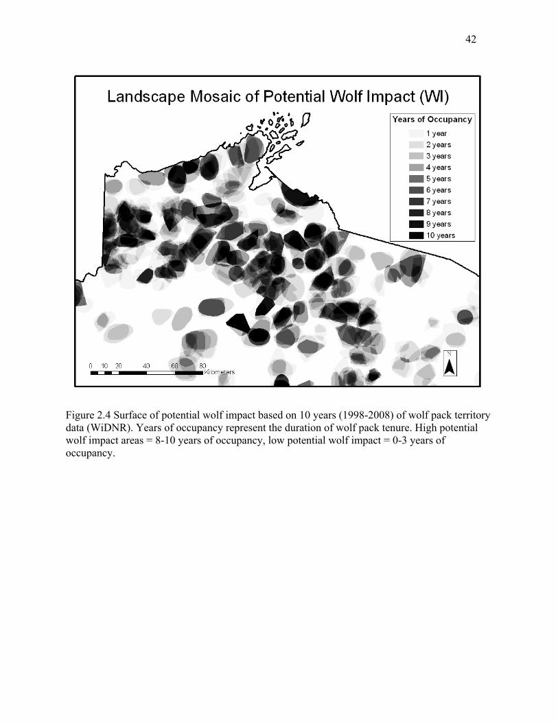
42

Figure 2.4 Surface of potential wolf impact based on 10 years (1998-2008) of wolf pack territory data (WiDNR). Years of occupancy represent the duration of wolf pack tenure. High potential wolf impact areas = 8-10 years of occupancy, low potential wolf impact = 0-3 years of occupancy.

43

0

10

20

30

40

50

60

70

80

90

Tree Shrub Forb Grass Sedge Fern

Perc

ent C

over

** *

Figure 2.5 Average percent cover of high and low potential wolf impact plots of six vegetation growth forms (forbs, shrubs, trees, ferns, grasses and sedges) with 95% confidence intervals. Values are averaged geometric means of cover classes ( 0-1%, 1-2%, 2-5%, 5-10%, 10-25%, 25-50%, 50-75%, 75-95%, 95-100%). Hatched bars represent areas with high potential wolf impact. Asterisks indicate significant differences (p < 0.05).

44

All Understory Plant Species (n=7) (a) (i)

Forbs (n=16) (b) (j)

Shrubs (n=16) (c) (k)

Area (m2)

0

10

20

30

40

50

0 200 400 600 800 1000-1

0

1

2

-2 -1 0 1 2 3

-1

0

1

2

-2 -1 0 1 2 30

10

20

0 200 400 600 800 1000

0

10

20

30

40

50

60

70

80

90

100

0 200 400 600 800 1000-1

0

1

2

-2 -1 0 1 2 3

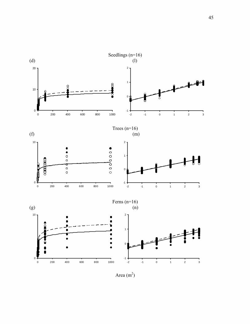
45

Seedlings (n=16) (d) (l)

Trees (n=16) (f) (m)

Ferns (n=16) (g) (n)

Area (m2)

-1

0

1

2

-2 -1 0 1 2 30

10

20

0 200 400 600 800 1000

0

10

0 200 400 600 800 1000-1

0

1

2

-2 -1 0 1 2 3

0

10

0 200 400 600 800 1000-1

0

1

2

-2 -1 0 1 2 3

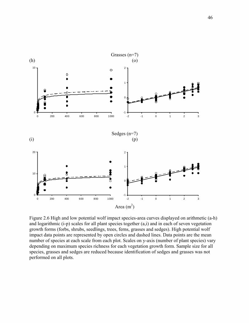
46

Grasses (n=7) (h) (o)

Sedges (n=7) (i) (p)

Area (m2) Figure 2.6 High and low potential wolf impact species-area curves displayed on arithmetic (a-h) and logarithmic (i-p) scales for all plant species together (a,i) and in each of seven vegetation growth forms (forbs, shrubs, seedlings, trees, ferns, grasses and sedges). High potential wolf impact data points are represented by open circles and dashed lines. Data points are the mean number of species at each scale from each plot. Scales on y-axis (number of plant species) vary depending on maximum species richness for each vegetation growth form. Sample size for all species, grasses and sedges are reduced because identification of sedges and grasses was not performed on all plots.

-1

0

1

2

-2 -1 0 1 2 30

10

0 200 400 600 800 1000

0

10

20

0 200 400 600 800 1000-1

0

1

2

-2 -1 0 1 2 3

47

CHAPTER 3

WOLF RECOVERY AND THE FUTURE OF WISCONSIN’S FORESTS:

A TROPHIC LINK?2


Forest Ecology and Management spring 2011

48

3.0 Abstract

The negative impacts of overabundant white-tailed deer (Odocoileus viginianus)

populations on understory plant community structure and species composition have been well

established. However, few studies have examined how the recovery of gray wolves (Canis lupus)

might moderate these effects. Wolves, which have been recolonizing central Wisconsin since the

early 1990s, are known to alter both the foraging behavior and local density of white-tailed deer.

To test for evidence of indirect effects of wolves on understory woody plants, we first calculated

an index of potential wolf impact based on historic and current wolf territory data: the Weighted

Wolf Occupancy Duration Index (WWODI). We then performed intensive vegetation surveys

(n=38) in northern white cedar wetlands across a gradient of wolf impact. Our objective was to

evaluate the relationship between wolf pack tenure and woody stem density and species diversity

in this highly browse sensitive and speciose community. In addition, we evaluate the potential

for wolf recovery to alter the future canopy composition of northern white cedar wetlands.

Spearman rank correlations show the continuous presence of a wolf pack to be positively

and significantly correlated with seedling density (ρ = 0.602, p < 0.0001) species richness (ρ =

0.601, p < 0.0001), and Shannon’s diversity index (ρ = 0.584, p < 0.0001) of woody stems in the

50-100 cm height class. Surprisingly, moderately browsed species showed a stronger relationship

with WWODI than severely browsed species (ρ = 0.635, p < 0.0001 vs. ρ = 0.353, p < 0.05). We

propose two possible explanations for this discrepancy: 1) that even a few deer are able to

prevent recruitment of highly preferred species, and/or 2) sensitive species are now so rare that a

response to reduced browsing pressure is difficult to detect because of limited sample sizes.

Unpalatable or insensitive species showed no relationship with WWODI. Size classes above the

browse line also showed no relationship with WWODI.

49

Density of wild sarsaparilla (Aralia nudicaulis) and nodding trillium (Trillium cernuum),

two perennial forb species known to decline with increased deer density, were strongly positively

correlated with WWODI (ρ = 0.462, p < 0.005 and ρ = 0.479, p < 0.005 respectively). Other

measures of browse pressure (scape height of the blue-bead lily, Clintonia borealis, red maple

browse index, and deer density DMU-1) were unrelated to WWODI. Site specific estimates of

deer density continue to be a challenge in deer-vegetation studies, but our pilot study of un-

baited infrared digital trail cameras demonstrated a potential for providing deer visitation rates

and unambiguously confirmed substantial use of cedar stands by deer during spring and summer

months.

The gap in the size structure of woody stems characteristic of over-browsed understories

is less apparent in cedar wetlands with high wolf impact. However, regardless of wolf impact,

recruitment of cedar in our study area is very limited. As the mature cedar and other co-

dominants senesce, it is likely that these remnant forests will be replaced by balsam fir (Abies

balsamea) stands and speckled alder (Alnus incana subsp. rugosa) thickets.

Key Words: cedar wetlands, trophic cascade, deer browsing, wolf recovery, seedling recruitment, demographic inertia, Wisconsin

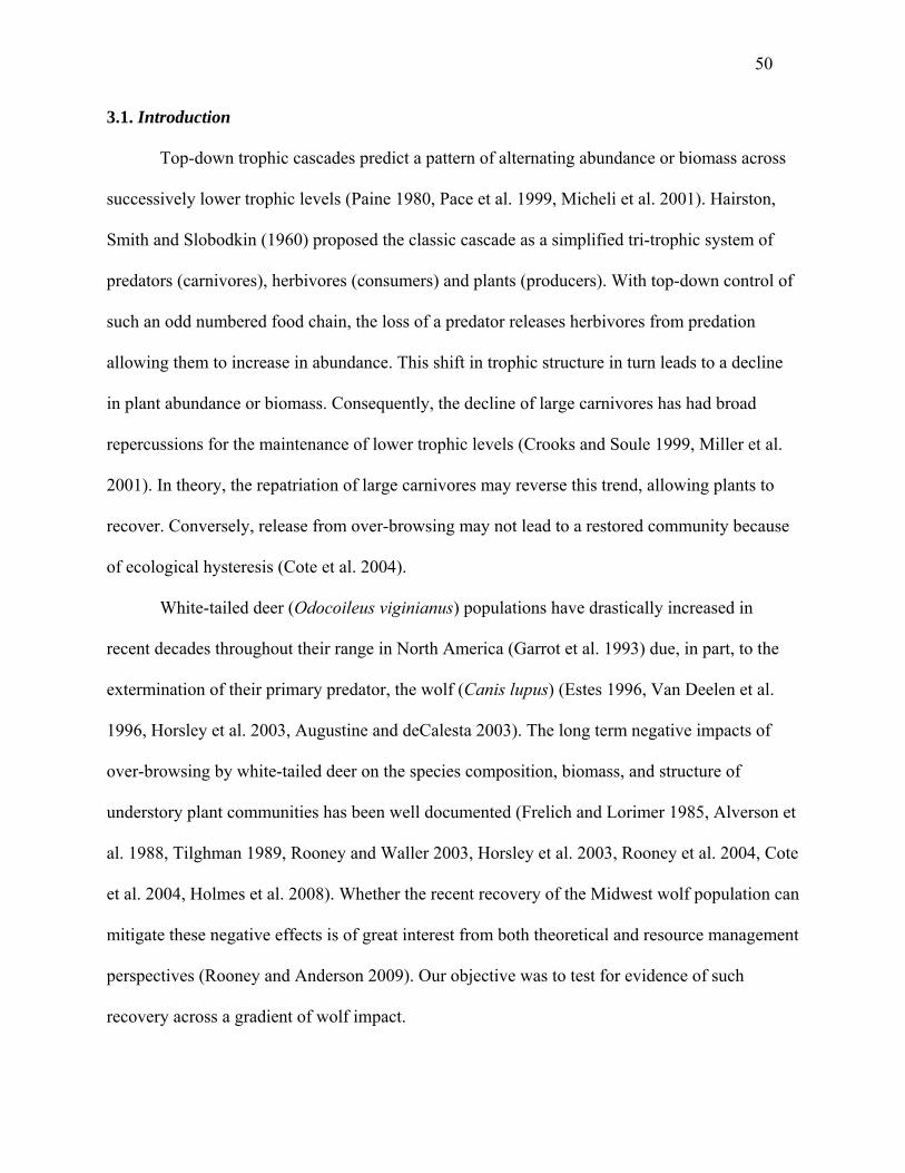
50

3.1. Introduction

Top-down trophic cascades predict a pattern of alternating abundance or biomass across

successively lower trophic levels (Paine 1980, Pace et al. 1999, Micheli et al. 2001). Hairston,

Smith and Slobodkin (1960) proposed the classic cascade as a simplified tri-trophic system of

predators (carnivores), herbivores (consumers) and plants (producers). With top-down control of

such an odd numbered food chain, the loss of a predator releases herbivores from predation

allowing them to increase in abundance. This shift in trophic structure in turn leads to a decline

in plant abundance or biomass. Consequently, the decline of large carnivores has had broad

repercussions for the maintenance of lower trophic levels (Crooks and Soule 1999, Miller et al.

2001). In theory, the repatriation of large carnivores may reverse this trend, allowing plants to

recover. Conversely, release from over-browsing may not lead to a restored community because

of ecological hysteresis (Cote et al. 2004).

White-tailed deer (Odocoileus viginianus) populations have drastically increased in

recent decades throughout their range in North America (Garrot et al. 1993) due, in part, to the

extermination of their primary predator, the wolf (Canis lupus) (Estes 1996, Van Deelen et al.

1996, Horsley et al. 2003, Augustine and deCalesta 2003). The long term negative impacts of

over-browsing by white-tailed deer on the species composition, biomass, and structure of

understory plant communities has been well documented (Frelich and Lorimer 1985, Alverson et

al. 1988, Tilghman 1989, Rooney and Waller 2003, Horsley et al. 2003, Rooney et al. 2004, Cote

et al. 2004, Holmes et al. 2008). Whether the recent recovery of the Midwest wolf population can

mitigate these negative effects is of great interest from both theoretical and resource management

perspectives (Rooney and Anderson 2009). Our objective was to test for evidence of such

recovery across a gradient of wolf impact.

51

Prior to European settlement, densities of white-tailed deer in the northern Great Lakes

Region were much lower because of extreme winters and extensive coverage of mature hemlock-

hardwood forests (Dahlberg and Guettinger 1956, Habeck and Curtis 1959, DelGuidice et al.

2009). The early successional communities and high edge density created by large-scale clear

cutting caused drastic increases in forage availability. Agriculture, deer baiting and fertilized

lawns and gardens have amplified these positive impacts on habitat quality for white-tailed deer.

When combined with the intentional eradication of large carnivores, these environmental

changes have led to severely inflated deer populations throughout the region. For most of the 20th

century, understory plant communities of northern Wisconsin have been subject to deer densities

that exceed pre-settlement conditions by 350-500% (Rooney and Waller 2003).

Comparisons between deer exclosures and adjacent browsed plots in both Wisconsin and

Michigan have shown drastic differences in the survival and reproductive success of preferred

browse species (Graham 1954, Dahlberg and Guettinger 1956, Stoeckeler, Strothman, and

Krefting 1957). Exclosure studies can be difficult to interpret because they provide only two

points of reference, comparing extremely high browsing pressure to non-existent browsing

pressure (Hobbs et al. 1996). Because deer-plant interactions were hypothesized to have non-

linear dynamics, more recent correlative (Alverson et al. 1988, Alverson and Waller 1997,

deCalesta 1997, Augustine and Jordan 1998, Cote et al. 2004, Holmes et al. 2008) and

manipulative studies (Tilghman 1989, Horsley et al. 2003) have explored variation in white-

tailed deer density across a gradient of deer impact in both space and time.

Evidence from these manipulative experiments in northern hardwood forests shows a

distinctive threshold pattern indicating that the diversity of forbs, shrubs and trees in seedling

size classes drastically decreases when deer density increases from moderate to high levels

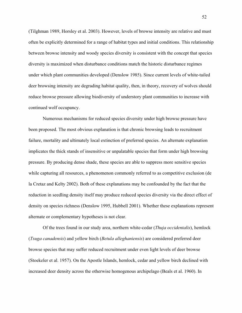
52

(Tilghman 1989, Horsley et al. 2003). However, levels of browse intensity are relative and must

often be explicitly determined for a range of habitat types and initial conditions. This relationship

between browse intensity and woody species diversity is consistent with the concept that species

diversity is maximized when disturbance conditions match the historic disturbance regimes

under which plant communities developed (Denslow 1985). Since current levels of white-tailed

deer browsing intensity are degrading habitat quality, then, in theory, recovery of wolves should

reduce browse pressure allowing biodiversity of understory plant communities to increase with

continued wolf occupancy.

Numerous mechanisms for reduced species diversity under high browse pressure have

been proposed. The most obvious explanation is that chronic browsing leads to recruitment

failure, mortality and ultimately local extinction of preferred species. An alternate explanation

implicates the thick stands of insensitive or unpalatable species that form under high browsing

pressure. By producing dense shade, these species are able to suppress more sensitive species

while capturing all resources, a phenomenon commonly referred to as competitive exclusion (de

la Cretaz and Kelty 2002). Both of these explanations may be confounded by the fact that the

reduction in seedling density itself may produce reduced species diversity via the direct effect of

density on species richness (Denslow 1995, Hubbell 2001). Whether these explanations represent

alternate or complementary hypotheses is not clear.

Of the trees found in our study area, northern white-cedar (Thuja occidentalis), hemlock

(Tsuga canadensis) and yellow birch (Betula alleghaniensis) are considered preferred deer

browse species that may suffer reduced recruitment under even light levels of deer browse

(Stoekeler et al. 1957). On the Apostle Islands, hemlock, cedar and yellow birch declined with

increased deer density across the otherwise homogenous archipelago (Beals et al. 1960). In

53

Michigan deer yards, Van Deelen et al. (1996) documented drastic declines in cedar, hemlock,

and yellow birch recruitment with concurrent increases in balsam fir (Abies balsamea), poplar

(Populus spp.), and maple (Acer spp.).

We chose to focus on northern white cedar stands due to the established link between

recruitment failure of cedar and white-tailed deer browsing intensity (Verne and Johnson 1986,

Alverson et al. 1988, Heitzman et al. 1999, Van Deelen 1999, Cornett et al. 2000, Rooney et al.

2001, Forester et al. 2008). Northern white cedar is a highly preferred browse species (Beals et

al. 1960, Ully et al. 1968) and lowland cedar stands have been intensively used by deer during

the winter months (Verme 1965) often sustaining deer yard densities from 30-40/km2. Thus, we

anticipated that recovery of shrubs and seedlings would be more easily detected in this uniquely

diverse and browse-sensitive community type.

With protection under the Endangered Species Act, wolves have been recolonizing

northern Wisconsin since the early 1970s, but had very limited distribution until the

1990s.(Wydeven et al. 1995, Wydeven et al. 2009). Hoskinson and Mech (1976) reported

observations that deer survival is higher on the edges of wolf territories as compared to their

centers. Wolves are less likely to hunt in these buffer zones so as to avoid potentially fatal





Increased vigilance of individual deer that do continue to forage within wolf territories is

also likely to reduce local impacts on woody browse species. By forcing deer to increase

movement and spend less total time browsing, the presence of wolves may alter the disturbance

54

regime experienced by local plant communities. Within occupied wolf territories, deer may no

longer be able to sit and browse one location until all preferred species become locally rare or

extinct.

We hypothesized that the recovery of wolves in Wisconsin has generated a mosaic of

deer browsing intensity as deer alter their foraging activity to avoid occupied wolf territories,

showing preference for the buffer zones between adjacent packs. Our first goal was to calculate

an index of potential wolf impact based on historic data of wolf pack territory extents. Our

primary objective was to test for a relationship between this index of potential wolf impact and

the structure, density, species diversity and species composition of woody stems in understory

communities of northern white cedar wetlands. Our secondary objective was to compare our

index of potential wolf impact with commonly used measures of deer browse intensity. Our final

objective was to predict future changes in canopy species composition of lowland cedar stands.

3.2. Methods

3.2.1 STUDY SITE


various state and county forests spanning 7 counties in north-central Wisconsin. The forests of

Northern Wisconsin are transitional between deciduous forests to the south and boreal forests to

the north (Pastor and Mladenoff 1992, Mladenoff et al. 1993). Annual air temperature in

northern Wisconsin averages 4º C, and mean annual precipitation ranges between 76 and 86 cm.

The freeze free period averages ~80 days, making for a short growing season. Snowfall

accumulation frequently exceeds 76 cm and this snow cover provides insulation for ground

vegetation (NOAA 1982).

55

Glaciation strongly influenced the soils and topography of Wisconsin. Soils are derived

from sandy loam glacial till, silt covered glacial till, and sandy outwash. With a maximum

elevation of 550 m, there is little topographic relief. The gently rolling terrain is inundated with

thousands of lakes and numerous wetlands. Terrestrial landscapes are comprised of 40%

deciduous forest types (dominated by sugar maple, Acer saccharum and paper birch, Betula

papyrifera), 9% coniferous, (dominated by white pine, Pinus resinosa, red pine, Pinus strobus,

and balsam fir, Abies balsamea), 8% mixed-coniferous-deciduous, and 7% early successional

(dominated by aspen, Populus tremuloides). Forested and emergent wetland communities cover

an additional 26% of the area (dominated by tamarack, Larix laricina and black spruce, Picea

mariana, and Labrador-tea, Ledum groenlandicum and leather leaf Chamaedaphne calyculata,

respectively). Northern-white cedar wetlands occupy less than 5% of the landscape but support a

large proportion of the regional biodiversity (WiDNR 1998).

Northern-white cedar wetlands develop on poorly-drained sites with a slight through-flow

of groundwater. These conditions elevate the pH and nutrient richness of the soil (Black and

Judziewicz 2008). Mature stands of white cedar are densely shaded with nearly closed canopies.

The combination of these environmental characteristics produces unique light regimes and soil

chemistry required by species restricted to this community type. Co-dominant trees in white

cedar wetlands include balsam fir, yellow birch (Betula alleghaniensis) and black ash (Fraxinus

nigra). Speckled alder (Alnus incana subsp. rugosa), hollies (Ilex mucronata and I. verticillata),

hazelnuts (Corylus spps.) and honeysuckles (Lonicera spps.) are common understory shrubs.

56

3.2.2 WOLF DATA

Wisconsin Department of Natural Resources (WiDNR) population estimates of wolves

were ascertained by live-trapping and radio tracking (Mech 1974, Fuller and Snow 1988), howl

surveys (Harrington and Mech 1982), and winter track surveys (Thiel and Welch 1981, Wydeven

et al. 1995). Territory extents were delineated using minimum convex polygons based on

radiolocations of collared wolves and other wolf sign (Wydeven et al. 1995, Wydeven et al.

2009). Depending on pack size and prey density, wolf territories in the Great Lakes Region can

range in size but average approximately 136 km2 (Wydeven et al. 2009). Wolf packs establish

and occupy territories that are patchily distributed across the landscape (Mladenoff et al. 1999).

The negative effect of wolves on deer abundance and foraging behavior is likely to be limited to

locations continuously occupied by wolf packs. Presumably, the impact of wolves increases with

the number of years the territory has been consistently occupied. Since pack size and territory

extent vary from year to year, this creates a mosaic of wolf impact intensity across the landscape.

Using GIS, we overlaid current wolf territories with historic territory extents back to

1995 (Wydeven and Wiedenhoeft 2008). Only sites that fell within the Chequamegon-Nicolet

National Forest, state or county forest boundaries were selected. Although wolves have

established territories outside of public lands, these territories are often located in agricultural or

industrial forest landscapes and anthropogenic sources of landscape change are likely to

confound any potential trophic effects of wolf recolonization. It was also difficult to locate and

obtain access to northern white cedar stands on private property. We categorized locations that

had been occupied for 0-3 years as low potential wolf impact areas, locations that had been

occupied for 5-6 years as moderate potential wolf impact areas and locations that had been

occupied for more than 8 years as high potential wolf impact areas.

57

Weighted wolf occupancy duration Index (WWODI) values were calculated by summing

the most recent 15 years of DNR wolf territory extent data (1993-2007 for vegetation plots

surveyed in 2008 and 1994-2008 for plots surveyed in 2009). Recent years were weighted more

strongly given the assumption that wolf occupancy in the distant past would have a weaker

impact on current browse intensity and therefore a weaker indirect effect on understory plant

communities. The most recent year of wolf occupancy (presence/absence of a wolf pack at each

location) was divided by 1, the next most recent year was divided by 1.1, and so on. Thus:

WWODI = Yt/1+ Yt-1/1.1 + Yt-2/1.2 + ……..Yt-15/2.4

where Yt is the current year of wolf occupancy and Yt-15 is the wolf occupancy 15 years ago.

Although we had hoped to calculate wolf density by dividing territory area by the number of

wolves in each pack, pack size data was not consistently collected for all years and all packs.

3.2.3 DEER DATA

White-tailed deer density data were obtained for each deer management unit (DMU) for

the year in which vegetation data were collected, either 2008 or 2009 (WiDNR 2009). WiDNR

calculates initial deer density estimates using the sex-age-kill method and then corrects for the

proportion of the DMU that is considered deer habitat (Millspaugh et al. 2006). Wisconsin

DMUs are vastly larger in area than the cedar stands and wolf pack territories they contain. Since

a deer density estimate for a given DMU is a single value intended to represent an average across

a very large heterogeneous area, it is unlikely that these values represent the site specific deer

density influencing the understory of isolated cedar stands. Unfortunately, this was the only

region-wide data available.

58

Un-baited infrared triggered cameras (ITCs) have been successfully used to estimate

local abundance of white-tailed deer (Roberts et al. 2006). In the early spring of 2009 (17th of

April), we set up 14 ITCs in vegetation plots that had been surveyed in 2008 (one camera per

plot). The cameras were faced into the plot to record deer visitations. All cameras were checked

in early summer (June 10th-12th) and removed from the field by August 21st. Observations were

divided into two sessions: spring (April 17th-June 10th), and summer (June 10th – August 21st).

Only 7 of the 14 cameras remained functional until they were retrieved in late summer. Leaf

River© digital trail cameras failed to capture images of deer due to a considerable delay between

animal detection and camera activation. Cuddeback© trail cameras performed very well. The

total number of deer captured by each Cuddeback© was then divided by the total number of days

the camera was operational for spring and summer sessions. Leaf River© trail cameras did not

produce usable data, reducing our sample size to n=7.

We measured site specific browse intensity on each vegetation plot for plots surveyed in

2008 (n=14). Browse intensity indices conformed to the sugar maple browse index (SMBI)

developed by Frelich and Lorimer (1985). Unfortunately, sugar maple seedlings were rare in the

northern white cedar wetlands and we attempted to substitute a red maple browse index (RMBI).

We collected data for additional indicators of browsing intensity such as flower scape height in

the blue-bead lily (Clintonia borealis), density of wild sarsaparilla (Aralia nudicaulis) and

density of nodding trillium (Trillium cernuum) at all plots (n=32). These forb species have been

shown to decline in areas of high deer density (Balgooyen and Waller 1995, Augustine and

deCalesta 2003). Scape height of blue-bead lily and the density of wild sarsaparilla and nodding

trillium are negatively related to browsing pressure, and so, according to a trophic cascade

response, should be positively related to WWODI. In contrast, Red Maple Browse index, deer

59

density DMU-1 and deer visitation day-1 are positively associated with browsing pressure and so

should be negatively correlated with WWODI.

3.2.4 VEGETATION DATA


Forest (USDA 2001) and various state and county forest datasets to identify stands characterized

as northern white cedar wetlands. White cedar stands of similar area and stand age were selected.

We used Hawth’s Tools to randomly place one vegetation plot within each pre-selected white

cedar stand. We surveyed a total of 38 cedar stands, 14 plots were completed in summer 2008

and 24 plots were completed in summer 2009.

Vegetation surveys follow the Carolina Vegetation Survey (CVS) protocol developed by

Peet et al. (1998). Understory woody stem surveys consisted of two 10 X 10 m modules per 200

m2 plot. For each module, woody stems were identified to species when possible, but sometimes

only to genus. Scientific names conform to Gleason and Cronquist (1991). Tallies of stems in

each height class for seedlings (10-50 cm, 50-100 cm, 100-137 cm) and each diameter class for

saplings and mature trees (0-1 cm, 1-2.5 cm, 2.5-5 cm, 5-10 cm, 10-15 cm, 15-20 cm, 20-25 cm,

25-30 cm, 30-35 cm, 35-40 cm and > 40 cm) were recorded for each module. For trees greater

than 40 cm d.b.h. we measured the exact d.b.h. to the nearest centimeter. Data from the 2

modules were then averaged to provide a single value for each plot (the average number of stems

of each species per size class). Basal area per plot was calculated for each tree species and scaled

up to basal area per hectare.

To compare the diversity of woody stem species with WWODI, we calculated the species

diversity index per plot, averaging values from the two modules. Diversity of woody species for

60

each size class was calculated using the Shannon-Weiner diversity index (H' = -[Σ(pi) (ln pi)]). A

simple linear regression model was fit to test for a relationship between species diversity and the

strength of potential wolf impact (WWODI).

3.2.5 LITERATURE REVIEW OF SPECIES SPECIFIC BROWSING RESPONSE

When assessing browsing response, it is important to consider both browse preference

(the relative desirability of the plant species to foraging white-tailed deer) and browse sensitivity

(the physical response of plant species to browsing events) of each species. For example, more

sensitive, preferred species such as red oaks (Quercus rubra), have displayed drastic differences

in seedling mortality rate, 34.6% for exposed seedlings compared to 3.2% for seedlings protected

from deer herbivory (Stange and Shea 1998). In contrast, sugar maple (Acer saccharum) also a

preferred species, can survive high browse pressure for many years without mortality

(Switzenberg et al. 1955, Stoeckler, Strothman, and Krefting 1957). At the extreme end, balsam

fir is rarely browsed and may in fact experience a competitive advantage when deer browsing

levels are high (Graham 1954). Understanding browse preference is complicated by the fact that

preference is relative and dependent on the available species in the area. For example, balsam fir

is not a preferred species in cedar wetlands, where it replaces cedar under high browsing

pressure, but is preferred on some islands where more palatable species are rare.

Table 3.1 shows a list of tree and shrub species found in northern white cedar stands of

north-central Wisconsin. Based on a review of the available literature, we assigned a browsing

response value to each species. Species that were observed to be browsed more often than their

abundance in the community would suggest were considered to be preferred. Species that were

more abundant inside exclosures were considered sensitive to deer browsing. Response values

61

ranged from -4 (recruitment failure) to +3 (competitive advantage). With few exceptions, browse

preference and sensitivity information for shrub species was limited. These browsing response

scores were used in the following analyses to determine which groups of woody stem species

showed a relationship with potential wolf impact.

3.3. Results

3.3.1 SPECIES RICHNESS AND POTENTIAL WOLF IMPACT

A one-way ANOVA was used to test for woody stem species richness differences among

high, moderate and low potential wolf impact (Figure 1). Species richness differed significantly

across the three levels of wolf impact for the three seedling size classes: 10-50 cm, F (2, 35) =

5.72, p = 0.007, 50-100 cm, F (2, 35) = 10.71, p < 0.0001, and 100-137 cm, F (2, 35) = 3.37, p =

0.05. Species richness did not differ for the two sapling size classes: 0-1 cm d.b.h., F (2, 35) =

1.41, p = 0.257, and 1-2.5 cm d.b.h., F (2, 35) = 0.32, p = 0.729.

3.3.2 WEIGHTED WOLF OCCUPANCY DURATION INDEX (WWODI)

The weighted wolf occupancy duration index ranged from 0.00 – 9.47 with an average

value of 4.66. These data are not normally distributed so they were compared to other variables

using Spearman rank correlations. Figure 3.2 shows the linear relationship (y = 0.0934x + 0.798,

r2 = 0.379, p<0.0001) between weighted wolf occupancy index values and Shannon’s diversity

index of all woody species 50-100cm in height at the plot level (n=38). Relationships between

WWODI and the diversity of woody stems in the other size classes were weaker, similar to the

species richness comparisons above. Despite considerable variability among sites, this strong

positive relationship was consistent and suggests an indirect positive trophic response to wolf

62

recovery. While a simple cumulative occupancy index, which ranged from 0-15, had a similar

relationship with diversity of woody species 50-100 cm (y = 0.0593x + 0.829, r2 = 0.356,

p<0.0001), the weighted index provided a slightly improved fit and was considered a logical

compromise between underestimating and overestimating the effect of historic wolf occupancy.

Time-weighted averages are a useful tool for reducing data to a single value for use in regression

analyses (Vanni and Layne 1997, Mörschel 1999).

3.3.3 SPECIES COMPOSITION

Northern white cedar averaged 84.5% of the total basal area (TBA) of all 38 vegetation

plots but ranged from 36.8%-99.0% (Table 3.2). Balsam fir, black ash, yellow birch, paper birch

and red maple comprised the majority of the remaining TBA (13.1% collectively). Black ash and

red maple were clearly co-dominant at some sites representing up to 49.1% and 35.7% of the

TBA respectively. Scattered eastern hemlock, black spruce, eastern white pine, tamarack and

white spruce occurred in a few plots but did not consistently constitute a significant portion of

the canopy.

The understory was often dominated by speckled alder or balsam fir. Hollies (Ilex spp.),

honeysuckles (Lonicera spp.), dogwoods (Cornus spp.), gooseberries (Ribes spp.), hazelnuts

(Corylus spp.), blueberries (Vaccinium spp.) and Labrador tea (Ledum groenlandicum) were

common in the understory but contributed little to basal area as few of them reached breast

height (with the exception of Ilex spp.). Sugar maple (Acer saccharum), mountain maple (Acer

spicatum), red oak (Quercus rubra), mountain ash (Sorbus spp.), American basswood (Tilia

americana), and American elm (Ulmus Americana) were found occasionally as seedlings in the

understory but were not found in the canopy.

63

3.3.4 CANOPY COVER, DEMOGRAPHIC INERTIA, AND WWODI INFLUENCE ON SEEDLING DENSITY

Spearman rank correlations of all woody species suggest that the density of woody stems

in the first size class (10-50cm in height) is related primarily to canopy cover (ρ = -0.559, p <

0.0005) and secondarily to WWODI (ρ = 0.404, p < 0.05) which we associate with a potential

reduction in browsing pressure (Table 3.3a). Canopy cover is inversely related to available light

explaining the strong negative relationship between woody stem density and canopy cover. At

the second size class (50-100cm in height), WWODI has the strongest relationship with woody

stem density (ρ = 0.602, p < 0.0001) followed by demographic inertia (ρ = 0.496, p < 0.005).

Demographic inertia is the density of woody stems in the preceding size class (size class 1 in this

case). At this stage, canopy cover is no longer an important factor suggesting that light

availability influences germination success but demographic inertia and disturbance intensity

(i.e. browsing pressure) determine establishment and recruitment. As the woody stems escape the

browse line, beyond size class 3 (100-137cm in height), demographic inertia surpasses WWODI

and continues to be the dominant factor driving woody stem density for the sapling size classes

(0-2.5cm dbh).

We anticipated that the species likely to experience recruitment failure at high levels of

browsing pressure (i.e. yellow birch, red oak, hemlock and cedar) would have an even stronger

relationship with WWODI than moderately browsed species. However, the relationship was in

fact weaker, but still significant for the 2nd and 4th size classes (Table 3.3b). When we grouped

species likely to gain a competitive advantage from browsing pressure (balsam fir, speckled alder

and spruce) the previously observed relationship with WWODI disappeared completely (Table

3.3c). The density of browsing insensitive species appear entirely dependent on canopy cover

and demographic inertia. The strongest relationship with WWODI was in fact found with the

64

woody stem density of moderately impacted species (the species scoring between 1and -2 for

browsing response in Table 3.1). The positive relationship between density of saplings in size

class 5 and canopy cover is likely due to saplings of this size contributing to canopy cover and

providing additional shade at the height at which densiometer readings were taken.

When we separated shrub species from tree species (having removed species that are

likely to experience a competitive advantage with increased browse pressure: balsam fir,

speckled alder and spruce), additional patterns emerged. Density of shrubs in size class 1 is much

more strongly related to canopy cover than tree seedlings of the same size (r = -0.643, p < 0.0001

compared to r = -0.078, p = 0.643). This likely reflects the fact that most of the tree species are

shade tolerant. WWODI is the only variable strongly correlated with shrub density at size class 2

(r =0.626, p < 0.0001). In contrast, while the relationship between WWODI and seedling stem

density is somewhat weaker (r = 0.415, p < 0.01 ), it transmits up through to the 4th size class.

Few individual shrubs reach size class 4 so this difference may be due to a smaller sample size.

When we analyzed species independently, and compared the density of woody stems of

each species to WWODI, more specific associations became apparent (Table 3.4). More than

half of the shrub species were strongly related to WWODI, while less than a third of the tree

species showed a significant correlation. The densities of quaking aspen (Populus tremuloides) ,

velvet-leaf blueberry (Vaccinium myrtilloides), and mountain holly (Ilex mucronata) were

negatively correlated with WWODI implying that they may in fact gain a competitive advantage

with high browsing pressure. Among the tree species, the density of woody stems of sugar

maple, striped maple, yellow birch, and black ash were significantly positively correlated with

WWODI. Among the shrubs, densities of red osier dogwood (Cornus stolonifera), American and

beaked hazelnut (Corylus americana and C. cornuta), American and swamp fly honeysuckle

65

(Lonicera canadensis, and L. oblongifolia), alder-leaf buckthorn (Rhamnus alnifolia), and

gooseberry species (Ribes spp.) were significantly positively correlated with WWODI.

Few studies have addressed the relative browsing preference and sensitivity of shrub

species (see Table 3.1). Our data suggest that they may be even more sensitive than many tree

species (assuming an indirect effect of wolves on plants via a trophic cascade mechanism).

Given that shrub species do not benefit from a constant seed rain from the canopy, over-

browsing of these species could quickly lead to local stand-level extinction. Some species may

simply have been too rare to show a definite relationship with WWODI one way or the other.

Density of alder and balsam fir may reflect historic browsing pressure and represent an aspect of

the community that will not change with reduced browsing pressure (consistent with the theory

of ecological hysteresis).

3.3.5 RELATIONSHIP BETWEEN WWODI AND BROWSING INTENSITY

Table 3.5 shows Spearman rank correlations between WWODI and six commonly used

measures of browse intensity. The lack of a relationship between WWODI and deer density

DMU-1 (r = -0.019, p = 0.909) is not surprising given the disparity in scale between these two

variables. High impact wolf sites were intentionally paired with the closest low wolf sites during

the first season so most high and low wolf impact sites are located within the same DMU (which

explains the U-shaped pattern in Figure 4d). The variation in local deer density within a DMU is

likely to be great given the average size of DMUs in Wisconsin (1,200 km2) and the variability in

available forage and (presumably) predator pressure.

The red maple browse index (based on the proportion of browsed stems relative to

available stems) also had no apparent relationship with WWODI (r = -0.197, p = 0.540). Not all

66

of the plots had enough red maple to calculate a browse index (n=12). The index only varied

from 0.707 to 0.879 suggesting that all red maple seedlings were heavily browsed regardless of

wolf occupancy. The high wolf impact areas had a slightly lower browse index on average

(0.783 compared to 0.794), but the difference was not significant. Red maple may not be as good

of an indicator of browsing intensity as sugar maple. Many of the low wolf impact sites had no

red maple, and it is possible that red maple is more likely to suffer mortality under heavy browse

pressure compared to sugar maple. For future studies, it may be preferable to measure browse

intensity in an adjacent stand with sufficient sugar maple to calculate SMBI.

The camera surveys indicated a negative relationship between deer visitation day-1 and

WWODI (Figure 4), but the relationship was not significant (ρ = -0.270, p = 0.558) most likely

due to the small sample size (n=7). Local resource managers expressed the opinion that deer

would not be found in cedar stands during spring and summer because these habitats were

primarily used by deer during the winter months. Our camera survey showed irrefutable evidence

that deer are using these habitats in the spring and summer. Our images also confirmed that deer

are browsing both woody stem and herbaceous growth in these habitats throughout the growing

season. Sixty-four images of deer were captured by the 7 Cuddeback trail cameras in the 128

days that the cameras were on.

Average scape height of the blue bead lily was also unrelated to WWODI (ρ = 0.378, p =

0.279). Only 10 of the 38 plots contained flowering blue-bead lilies making it a poor indicator

species. In contrast, density of sarsaparilla and nodding trillium were strongly positively

correlated with WWODI (ρ = 0.462, p < 0.005 and ρ = 0.479, p < 0.005 respectively). The

relationship between density of these sensitive species and WWODI appears curvilinear

67

indicating a threshold in time (between 6 and 7 years of wolf occupancy) beyond which these

species begin to recover from browsing.

3.3.6 WOLF RECOVERY AND FUTURE CEDAR STAND COMPOSITION

On average, there was no significant difference in cedar seedling density between high

and low wolf impact areas across all size classes (Figure 4a). Even at the smallest size class

cedar density was more related to canopy cover (ρ = -0.617, p < 0.0001) than to WWODI (ρ =

0.187, p = 0.261). Black ash, which is not considered a highly preferred species, shows a clear

pattern suggesting a release from browse pressure in high wolf impact areas (Figure 4b). Black

ash woody stems in the first 4 size classes were 200-300% more abundant in high wolf impact

areas, however the difference was only significant at the smallest size class (High wolf = 780 ha-

1, and Low wolf = 197 ha-1, p = 0.05). Historically, black ash has been replaced by northern

white cedar since the adults are less shade tolerant than the slower growing but shade tolerant

white-cedar (Gates 1942). A similar but even stronger pattern is seen for yellow birch, a more

preferred species (Figure 4c). For this species, the first two size classes show significantly higher

densities of woody stems in high wolf impact areas. No difference was observed in the density of

balsam fir between high and low wolf areas (Figure 4d). Although black spruce, an unpalatable

species, appears more abundant in low wolf areas across early size classes, these differences

were not significant (Figure 4e).

3.4. Discussion

Top down effects are likely to attenuate (Schmitz et al. 2000), showing strong direct

effects (of carnivores on herbivores) but weaker indirect effects (of carnivores on plants and

68

other trophic levels). Some evidence suggests that more complex food webs typically dampen

the strength of trophic cascades (Polis and Strong 1996). The recovery of a top predator may

cause an initial pulse of environmental change that eventually subsides. Alternatively, it may

take many years to reverse the impacts of decades of chronic browsing by ungulates maintained

at population densities far above their historic numbers. Additionally, ecologically effective

densities of wolves may only recently have been reached (Soule et al. 2003).

We found that moderate wolf impact sites (5-6 years of wolf pack occupancy) had woody

stem species richness values intermediate between high and low wolf sites but that these sites

were not significantly different from either low or high wolf impact sites (Figure 1). Thus, a time

lag of at least 8 years may be required before trophic effects of wolf recovery manifest in an

easily detectable way. Will changes continue at the same pace, accelerate or asymptote?

Nonlinear dynamics can often develop with plant-herbivore interactions contingent upon

historical events and associated time lags (Cote et al. 2004). White cedar wetlands are relatively

sensitive to browsing by white-tailed deer and it is likely that other forest-cover types will

display lag times of different lengths. These lag times in trophic effects will depend on the

relative sensitivity and resilience of forest-cover types and their individual constituent species to

browsing pressure.

Regeneration of canopy dominants in the Great Lakes Region is strongly dependent on

the probability that their seedlings will survive browsing by white-tailed deer. White-tailed deer

browse the apical meristem of preferred seedlings which stunts plant growth and prevents

seedlings from escaping the browse zone (Gill and Beardall 2001). Browsing also reduces root

carbon reserves that are normally allocated to chemical defenses and future growth (Bryant et al.

1983). Chronic browsing can therefore produce a positive feedback loop since seedlings are

69

maintained at accessible heights and lack chemical defenses (Peinetti et al. 2001). As fewer and

fewer individuals survive past the seedling size classes, a gap develops in the population

structure of sensitive species, a pattern which is characteristic of heavily browsed forests

(Leopold et al. 1943, Whitney 1984). We anticipated that this gap would be more pronounced in

areas with high browsing pressure and by extension (given indirect effects) low potential wolf

impact.

Under high browsing pressure, early successional forests may also transition toward

dominance by nitrogen-fixing species such as Alnus spp. (Kill and Bryant 1998). Forested

wetlands in Wisconsin often develop thick understories of speckled alder (Alnus incana ssp.

rugosa) an actinorhizal shrub that forms a symbiotic relationship with N2-fixing actinomycetes

of the genus Frankia (Furlow 1979). It is likely that areas with historically higher browse

pressure will in fact have greater densities of speckled alder which serves to suppress other

understory species. Once these stands develop, it is unlikely that reducing browse pressure will

reverse this state. Indeed, densities of speckled alder had no relationship with WWODI across all

size classes. As the cedar and other co-dominants senesce, it is likely that these remnant lowland

cedar forests will be replaced by balsam fir stands and alder thickets.

Complicating the issue of recovery from browsing disturbance is the fact that ecological

systems display the potential for multiple stable states (Holling 1973, May 1977). Early

indications of alternate stable states and their potential drivers arose from investigations of

degraded rangelands (Noy-Meir 1975, Hart and Norton 1988). In the range management

literature, a degraded state is defined as a lower or less desirable state that can not be returned to

its former state without intensive management effort (Friedel 1991). Once a system has crossed

the threshold into an alternate stable state, simply reducing the disturbance intensity (grazing

70

pressure) may be insufficient to achieve management goals (Laycock 1991). While these

concepts developed out of range science, they are likely applicable to deer-vegetation

relationships as well (Stromayer and Warren 1997).

Despite this positive relationship between WWODI and woody stem density and

WWODI and species diversity, few of the canopy species in our vegetation plots appear to be

successfully recruiting individuals into the sapling size classes (with the exception of balsam fir)

(Figure 4a-e). In particular, cedar recruitment is extremely low. Lowland cedar may be slow to

respond to release from browse pressure simply because cedar seedlings grow extremely slowly,

typically requiring 10 years to reach 30 cm in height and 30 years to attain 3 m (Rooney et al.

2001). Based on their study of upland cedar stands in Minnesota, Cornett et al. (2000)

recommend protecting cedar seedlings from deer herbivory for 30-50 years in order to allow

them to escape the browse zone and successfully recruit seedlings taller than 2.1 meters.

Recruitment failure of cedars implies that recovery of northern white cedar stand

understories may not be possible and indicates future stand level replacement by balsam fir and

speckled alder. Mladenoff and Stearns (1993) have argued that the region-wide decline of

hemlock is unlikely to be a result of any one factor but instead a suite of interacting factors

including disturbance regimes, climate change, hemlock life history, ecosystem processes and

historical land use. They suggest that the effects of deer browsing are simply a local phenomenon

where deer are heavily concentrated. Their caveat against assuming a single cause of recruitment

failure may apply in part to northern white-cedar as well, but browsing clearly poses a major

constraint (Rooney et al. 2001). For example, Cornett et al. (2000) showed that browsing by

white-tailed deer was the major factor driving the lack of cedar seedlings greater than 25 cm tall.

Over a period of three years, Cornett et al. (2000) recorded that 76% of planted northern white

71

cedar seedlings in upland stands of northeastern Minnesota had been browsed at least once.

Except in exclosures, cedar seedlings between 30 cm and 1.3 m tall, representing the range of

seedling heights subject to deer browsing (Beals et al. 1960, Saunders and Puettman 1999), were

completely absent.

Woody species which are both highly preferred by deer and sensitive to deer browsing

may now be so rare that we can no longer detect their response to changes in browse pressure

(Russell et al. 2001). In addition, there is evidence that even low deer densities can keep

preferred species from recruiting because deer will always preferentially feed on these species

(Kamler et al. 2010). This may explain why we observed a stronger association between

WWODI and moderately browsed species than between WWODI and species likely to

experience recruitment failure with chronic browsing (cedar, hemlock, yellow birch).

At this time, it appears that the restructuring of understory communities caused by

decades of chronic deer herbivory may have resulted in an alternate stable state (Stromayer and

Warren 1997, Augustine et al. 1998, Carpenter 2001, Scheffer et al. 2001). Ecosystem changes in

deer yards such as soil compaction, increased peat decomposition and decreased water retention

have led to hydric forest conditions being replaced by mesic forest conditions (Van Deelen et al.

1996). These associated changes are likely to have strong effects on understory plant

communities that may not be reversible even under reduced browsing conditions (Van Deelen et

al. 1996). However, areas with high potential wolf impact do seem to support understory

communities more similar to historic plant communities as described by Curtis (1959) in that the

continuous presence of a wolf pack was associated with higher species diversity.

Site specific estimates of deer density continue to be a challenge in deer-vegetation

studies. Our camera surveys displayed great potential for detecting local variability in browsing

72

pressure. With a grid or array of cameras at multiple sites, combined with comparisons with

thermal infrared sensing techniques to calibrate density estimates, we believe these un-baited low

maintenance infrared triggered camera surveys can generate a very useful dataset. More

extensive ITC surveys of deer combined with the vegetation surveys and wolf territory data used

here would provide us with the ability to test for reciprocal relationships between wolves, deer

and vegetation which are needed to show definitive evidence of a trophic cascade.

3.5. Conclusion

The loss of wolves as a keystone predator has contributed to a less desirable state for

understory plant communities in northern white-cedar wetlands. Our data suggests that the

recovery of wolves in northern Wisconsin can partially reverse this trend, at least in specific

community types where wolf packs have been continuously present for at least 8 years. Whether

these observed differences in vegetation patterns are due to direct predation on ungulates

(density mediated indirect effects) or to the indirect effect of wolves on deer foraging behavior

(trait mediated indirect effects) continues to be hotly debated (Ripple and Beschta 2004, Beyer et

al. 2007, Creel and Christianson 2009, Kaufmann et al. 2010) and is beyond the scope of this

study.

We suspect, however, that density mediated indirect effects may be unlikely given that

the current Wisconsin wolf population, which has grown to ~620 individuals (Wydeven and

Wiedenhoeft 2009), has the capacity to take only ~11,000 deer per year. There are an estimated

390,000 deer in the northern forests of Wisconsin (posthunt), so region-wide effects of wolf

recovery on deer populations are unlikely to manifest in the short term. The reintroduction of

wolves to Yellowstone National Park (YNP) has shown that foraging prey species alter their

73

spatial use of available habitat in the presence of top predators (Ripple et al. 2001, Ripple and

Beschta 2003) and also reduce the amount of time allocated to foraging activities due to

increased vigilance (Lima and Dill 1990, Laundré et al. 2001). Thus, trait mediated indirect

effects may be the more likely mechanism responsible for higher density and diversity of woody

stems in high impact wolf areas.

Total trophic-level biomass, a sufficient response variable for aquatic systems, may be an


Recent evidence suggests that the indirect effects of predators in terrestrial systems are much

stronger on plant species diversity than on plant biomass, and that these changes in species

composition and evenness have strong effects on ecosystem properties (Schmitz 2006). Thus, we

need to rethink how we address trophic cascades in terrestrial systems as opposed to

characterizing them as weaker examples of aquatic cascades (sensu Strong 1992, Halaj and Wise

2001, Shurin et al. 2002). If we fail to do so, we risk measuring the wrong plant response

variables and missing evidence of ecologically important trophic cascades in terrestrial systems.

For northern white-cedar wetlands, we found density and species diversity of woody

stems 50-100cm tall to be ideal plant response variables with which to measure release from

browsing pressure, especially when allowances were made for variability in species specific

browsing response. The gap in the size structure of woody stems characteristic of over-browsed

understories was less apparent in cedar wetlands with high potential wolf impact. However,

regardless of WWODI, recruitment of cedar in lowland cedar stands in our study area continues

to be very limited. Alverson et al. (1988) concluded that deer densities need to be maintained

below 1-2/km2 in order to sustain the diversity of native Wisconsin plants. In our study area,

maximum deer densities of 13/km2 and above are common. It is unlikely that the recovery of the

74

wolf population alone will reduce the deer population to densities recommended by Alverson et

al. (1988). However, as the proportion of early successional forests decreases across the Great

Lakes Region, reduced forage, when combined with predation, may cause deer densities to

naturally decline.

75

REFERENCES Alverson, W. S., Waller, D. M. and S. L. Solheim. 1988. Forests too deer - edge effects in northern Wisconsin. Conservation Biology 2:348-358. Alverson, W. S., and D. M. Waller. 1997. Deer populations and the widespread failure of hemlock regeneration in northern forests. Pages 280-297 in W. J. McShea, H. B. Underwood, and J. H. Rappole, editors. The science of overabundance: deer ccology and population management. Smithsonian Institute Press, Washington, D.C., USA. Anderson, R. C. and A. J. Katz. 1993. Recovery of browse-sensitive tree species following release from white-tailed deer (Odocoileus virginianus) Zimmerman browsing pressure. Biological Conservation 63:203-208. Augustine, D. J., and P. A. Jordan. 1998. Predictors of white-tailed deer grazing intensity in fragmented deciduous forests. Journal of Wildlife Management 62:1076-85. Augustine, D. J., and D. DeCalesta. 2003. Defining deer overabundance and threats to forest communities: from individual plants to landscape structure. Ecoscience 10:472-86. Balgooyen, C.P. and D.M. Waller. 1995. The use of Clintonia borealis and other indicators to gauge impacts of white-tailed deer on plant communities in northern Wisconsin, USA. Natural Areas Journal 15:308-318. Beals, E.W., Cottam G., and R.J. Vogel. 1960. Influence of deer on vegetation of the Apostle Islands, Wisconsin. Journal of Wildlife Management 24:68-80. Beyer, H. L., E. H. Merrill, N. Varley, and M. S. Boyce. 2007. Willow on Yellowstone’s northern range: evidence for a trophic cascade? Ecological Applications 17:1563-1571. Black, M.R. and E.J. Judziewicz, 2008. Wildflowers of Wisconsin and the Great Lakes Region. The University of Wisconsin Press, Madison, Wisconsin. Bryant, J. P., F. S. Chapin, III, and D. R. Klein. 1983. Carbon/nutrient balance of boreal plants in relation to vertebrate herbivory. Oikos 40:357-368. Conover, M.R. and Kania, G.S. 1988. Browsing preference of white-tailed deer for different ornamental species. Wildlife Society Bulletin 16:175-179. Cornett, M. W., Frelich, L.E., Puettmann K.J., and P. B. Reich. 2000. Conservation implications of browsing by Odocoileus virginianus in remnant upland Thuja occidentalis forests. Biological Conservation 93:359-369. Cote, S.D., Rooney, T.P., Tremblay, J.P., Dussault, C. and D.M. Waller. 2004. Ecological impacts of deer overabundance. Annual review of Ecology, Evolution and Systematics 35:113-147.

76

Creel, S., and D. Christianson. 2009. Wolf presence and increased willow consumption by Yellowstone elk: implications for trophic cascades. Ecology 90:2454-2466. Crooks, K. R. and M. E. Soulé. 1999. Mesopredator release and avifaunal extinctions in a fragmented system. Nature 400: 563-566. Curtis, J. T. 1959. The vegetation of Wisconsin. University of Wisconsin Press, Madison. Dahlberg, B. L., and R. C. Guettinger. 1956. The white-tailed deer in Wisconsin. Wisconsin Conservation Department, Madison, Wisconsin, USA. DelGuidice, G.D., K. R. McCaffery, D.E Beyer, Jr. and M. E. Nelson. 2009. Prey of wolves in the Great Lakes Region. Pages 155-173 in A.P. Wydeven, T. R. Van Deelen, and E.J. Heske, editors. Recovery of Wolves in the Great Lakes Region of the United States: An Endangered Species Success Story. Springer, New York, NY, USA. Denslow, J. S. 1985. Disturbance-mediated coexistence of species. Pages 307-323 in S. T. A. Pickett and P. S. White, editors. The ecology of natural disturbance and patch dynamics. Academic Press, New York, New York, USA. Denslow, J. S. 1995. Disturbance and Diversity in Tropical Rain Forests: The Density Effect. Ecological Applications 5: 962-968. Estes, J. A. 1996. Predators and Ecosystem Management. Wildlife Society Bulletin 24:390-396. Furlow, J. J. 1979. The systematics of American species of Alnus (Betulaceae). Rhodora 81:151-248. Frelich, L. E. and C. G. Lorimer. 1985. Current and predicted long-term effects of deer browsing in hemlock forests of Michigan, USA. Biological Conservation 34: 99-120. Friedel, M. H. 1991. Range condition assessment and the concept of thresholds: a review. Journal of Rangeland Management 44: 422-426. Fuller, T. K. and W. J. Snow. 1988. Estimating winter wolf densities using radiotelemetry data. Wildlife Society Bulletin 16:367-370. Gates, F. C. 1942. The bogs of northern Lower Michigan. Ecological Monographs 12:213-254. Garrott, R.A., P.J. White, and C.A. Vanderbilt White. 1993. Overabundance: An issue for conservation biologists? Conservation Biology 7: 946-949. Gleason, H. A., and A. Cronquist. 1991. Manual of vascular plants of northeastern U.S. and adjacent Canada. 2nd Ed. The New York Botanical Garden, Bronx, New York, USA.

77

Graham, S. A. 1954. Changes in northern Michigan forests from browsing by deer. Transactions of the Nineteenth North American Wildlife Conference 19: 526-533. Habeck, J.R. and J. T. Curtis. 1959. Forest cover and deer population densities in early northern Wisconsin. Trans. Wis. Acad. Sci., Arts, & Letters 48:49-56. Halaj, J. and D. H. Wise. 2001. Terrestrial trophic cascades: how much do they trickle? American Naturalist 157(3): 262-281. Harrington, F. H. and L. D. Mech. 1982. An analysis of howling response parameters useful for wolf pack censusing. Journal of Wildlife Management 46:686-693. Hart, R. H. and B. E. Norton. 1988. Grazing management and vegetation response. Pages 493-525 in P.T. Tueller, editor. Vegetation science applications for rangeland analysis and management. Kluwer Academic Publishing Company, Boston, Massachusetts, USA. Hobbs, N. T. 1996. Modification of ecosystems by ungulates. Journal of Wildlife Management 60:695-713. Holling, C. S. 1973. Resilience and stability of ecological systems. Annual Review of Ecology Evolution and Systematics 4:1-23. Holmes, S. A., Curran, L. M., and K. R. Hall. 2008. White-tailed Deer (Odocoileus virginianus) alter herbaceous species richness in the Hiawatha National Forest, Michigan, USA. American Midland Naturalist 159:83-97. Horsley, S. B., Stout S. L. and D. S. deCalesta. 2003. White-tailed deer impact on the vegetation dynamics of a northern hardwood forest. Ecological Applications 13:98-118. Kauffman, M. J., Brodie, J. F. and E. S. Jules. 2010. Are wolves saving Yellowstone's aspen? A landscape-level test of a behaviorally mediated trophic cascade. Ecology 91:2742-2755. Laycock, W. A. 1991. Stable states and thresholds of range condition on North American rangelands: a viewpoint. Journal of Rangeland Management 44: 427-433. Leopold, A., Sowls, L. K., and D. L. Spencer. 1947. A survey of overpopulated deer range in the United States. Journal of Wildlife Management 11:162-77. May, R. M. 1977. Thresholds and breakpoints in ecosystems with a multiplicity of stable states. Nature 269:471-477. Mech, L.D. 1974. Current techniques in the study of elusive wilderness carnivores. Pages 315-322 in Proceedings of the XIth International Congress of Game Biologists, Stockholm, Sweden. Mech, L. D. 1977. Wolf-pack buffer zones as prey reservoirs. Science 198: 320-321.

78

Mech, L. D. 1994. Buffer zones of territories of gray wolves as regions of intraspecific strife. Journal of Mammalogy 75: 199-202. Millspaugh, J. J., Boyce, M. S., Diefenbach, D. R., Hansen, L. P., Kammermeyer, K., and J. R. Skalski. 2006. An evaluation of the SAK model as applied in Wisconsin. http://www.dnr.state.wi.us/org/land/wildlife/hunt/deer/SAKreport.pdf: Wisconsin Department of Natural Resources, 2006. Mladenoff, D. J., M. A. White, J. Pastor, and T. R. Crow. 1993. Comparing spatial pattern in unaltered old-growth and disturbed forest landscapes. Ecological Applications 2:294-306. Mörschel, F. M. 1999. Use of climatic data to model the presence of oestrid flies in caribou herds. The Journal of Wildlife Management 63:588-593. NOAA 1982. Climate of Wisconsin: climatography of the United States, No. 60. National Climatic Data Canter, Asheville, North Carolina, USA. Noy-Meir, I. 1975. Stability of grazing systems: an application of predator-prey graphs. Journal of Ecology 63:459-481. Paine, R. T. 1980. Food webs: linkage, interaction strength and community infrastructure. Journal of Animal Ecology 49:667-685. Pastor, J. and D. J. Mladenoff. 1992. The southern boreal-northern hardwood border. Pages 216-240 in H. H. Shugart, R. Leemans and G. B. Bonan, editors. A systems analysis of the global boreal forest. Cambridge University Press, Cambridge, UK. Peet, R. K., Wentworth, T. R., and P. S. White. 1998. A flexible, multipurpose method for recording vegetation composition and structure. Castanea 63:262-274. Peinetti, H. R., R. S. C. Menezes, and M. B. Coughenour. 2001. Changes induced by elk browsing in the aboveground biomass production and distribution of willow (Salix monticola Bebb): their relationships with plant water, carbon, and nitrogen dynamics. Oecologia 127:334-342. Ripple, W.J., and R.L. Beschta. 2004. Wolves and the ecology of fear: can predation risk Structure ecosystems? Bioscience 54:755-766. Roberts, C. W., Pierce, B. L., Braden, A. W., Lopez, R. R., Silvy, N. J., Frank, P. A., and D. Ransom. 2006. Comparison of camera and road survey estimates for white-tailed deer. Journal of Wildlife Management 70:263-267. Rooney, T. P., and D. Anderson. 2009. Are wolf-mediated trophic cascades boosting biodiversity in the Great Lakes region? Pages 205–215 in A. P. Wydeven, T. R. Van Deelen, and E. J. Heske, editors. Recovery of gray wolves in the Great Lakes region of the United States. Springer, New York, NY, USA.

79

Rooney, T. P., and D. M. Waller. 2003. Direct and indirect effects of white-tailed deer in forest ecosystems. Forest Ecology and Management 181:165-176. Rooney, T. P., S. M. Wiegmann, D. A. Rogers, and D. M. Waller. 2004. Biotic impoverishment and homogenization in unfragmented forest understory communities. Conservation Biology 18:787-798. Schmitz, O.J., Hamback, P.A., and A. P. Beckerman. 2000. Trophic cascades in terrestrial systems: a review of the effects of carnivore removals on plants. American Naturalist 155:141-153. Schmitz, O. J., Krivan, V., and O. Ovadia. 2004. Trophic cascades: the primacy of trait-mediated indirect interactions. Ecology Letters 7:153-163. Schmitz, O. J. 2006. Predators have large effects on ecosystem properties by changing plant diversity, not plant biomass. Ecology 87:1432-1437. Shurin, J. B., Borer, E. T., Seabloom, E. W., Anderson, K., Blanchette, C. A., Broitman, B. et al. 2002. A cross-ecosystem comparison of the strength of trophic cascades. Ecology Letters 5:785-791. Soulé, M. E., Estes, J. A., Berger, J., and C. M. Del Rio. 2003. Ecological effectiveness: conservation goals for interactive species. Conservation Biology 17:1238-1250. Stange, E. E., and K. L. Shea. 1998. Effects of Deer Browsing, Fabric Mats, and Tree Shelters on Quercus rubra seedlings. Restoration Ecology 6:29-34. Stoeckeler, J. H., R. 0. Strothman, and L. W. Krefting. 1957. Effect of deer browsing on reproduction in the northern hardwood-hemlock type in northeastern Wisconsin. Journal of Wildlife Management 21:75-80. Stormer, F.A. and W. A. Bauer. 1980. Summer forage use by tame deer in Northern Michigan. Journal of Wildlife Management 44:98-106. Strole, T.A., and R. C. Anderson. 1992. White-tailed deer browsing: Species preferences and implications for central Illinois forests. Natural Areas Journal 3:139-144. Stromayer, K. A. and R. J. Warren. 1997. Are overabundant deer herds in the Eastern United States creating alternate stable states in forest plant communities? Wildlife Society Bulletin 25:227-234. Switzenberg, D. F., T. C. Nelson, and B. C. Jenkins. 1955. Effect of deer browsing on quality of hardwood timber in northern Wisconsin. Forest Science 1: 61-67. Thiel, R. P. and R. J. Welch. 1981. Evidence of recent breeding activity in Wisconsin wolves. American Midland Naturalist 106:401-402.

80

Tilghman, N. G. 1989. Impacts of white-tailed deer on forest regeneration in northwestern Pennsylvania. Journal of Wildlife Management 53:524-532. USDA 2001. CDS Data Dictionary, USDA Forest Service, Region 9. Van Deelen, T. R., Pregitzer, K. S., and J. B. Haufler. 1996. A comparison of pre-settlement and present-day forests in two Northern Michigan deer yards. American Midland Naturalist 135:181-194. Vanni M. J., and C. D. Layne. 1997. “Top-down” trophic interactions in lakes: effects of fish on nutrient dynamics. Ecology 78:1-20. Werner, E. E., and S. D. Peacor. 2003. A review of trait-mediated indirect interactions in ecological communities. Ecology 84:1083-1100. Wetzel, J. F., Wambaugh, J. R. and J. M. Peek. 1975. Appraisal of white-tailed deer winter habitats in Northeastern Minnesota. The Journal of Wildlife Management 39:59-66. Whitney, G. G. 1984. Fifty years of change in the arboreal vegetation of Heart’s Content, an old-growth hemlock-white pine-northern hardwood stand. Ecology 65:403-408. Wisconsin Department of Natural Resources 1998. WISCLAND Land Cover, Wisconsin Department of Natural Resources, Madison, Wisconsin, USA. Wisconsin Department of Natural Resources 2009. Wisconsin DMU review: DMU reference materials. http://dmureview.editme.com/dmuref: Wisconsin Department of Natural Resources, 2009. Wydeven, A.P., R.N. Schultz, and R. P. Thiel. 1995. Monitoring a recovering wolf population in Wisconsin, 1979-1991. Pp 47-156 in L.N. Carbyn, S.H. Fritts and D.R. Seip, editors. Ecology and Conservation of Wolves in a Changing World. Canadian Circumpolar Institute, Occasional Publication No. 35, Edmonton, Alberta, Canada. Wydeven, A. P., and J. E. Wiedenhoeft. 2010. Gray wolf population, 2009-2010. Wisconsin Wildlife Surveys 16:140-155. Wydeven, A. P. J.E. Wiedenhoeft, R.N. Schultz, R.P. Thiel, R. L. Jurewicz, B.E. Kohn, and T. R. Van Deelen, 2009. History, population growth, and management of wolves in Wisconsin. Pages 87-105 in A.P. Wydeven, T. R. Van Deelen, and E.J. Heske, editors. Recovery of Wolves in the Great Lakes Region of the United States: An Endangered Species Success Story. Springer, New York, NY, USA.

81

Table 3.1 List of tree and shrub species identified in northern white cedar stands of north-central Wisconsin. Browsing response classes based on existing literature for the region. Unidentified and singular occurrence species were assigned to ‘Other’. Browsing response is the sum of browsing preference and sensitivity where Preferred = -2, Browsed = -1, Not preferred = 1, Sensitive = -2, Insensitive = 2 and Unclear = 0. ‘Unclear’ indicates either limited or conflicting data. Tree spp.

Browsing preference*

Browsing sensitivity

Browsing response

Abies balsamea Not Preferred 1,2,4 Insensitive 1,7,10 Competitive advantage (3) Acer rubrum Preferred 1,3 Unclear 1,10 Reduced recruitment (-2) Acer saccharum Browsed 1,5 Insensitive 1,6,7,10 Relatively unaffected (1) Acer spicatum Preferred 1,2 Insensitive 1 Relatively unaffected (0) Betula alleghaniensis Preferred 1 Sensitive 1,6,10 Recruitment failure (-4) Betula papyrifera Browsed 1,4 Unclear Relatively unaffected (-1) Fraxinus nigra Unclear Unclear Relatively unaffected (0) Larix laricina Unclear Sensitive 7 Reduced recruitment (-2) Picea spp. Not Preferred 4 Insensitive 7,8 Competitive advantage (3) Populus tremuloides Browsed 1,3 Insensitive 7 Relatively unaffected (1) Quercus rubra Preferred 5 Sensitive 9 Recruitment failure (-4) Sorbus spp. Preferred 1,2 Unclear Reduced recruitment (-2) Thuja occidentalis Preferred 1,4 Sensitive 7,8,9 Recruitment failure (-4) Tilia americana Preferred 1,5 Unclear Reduced recruitment (-2) Tsuga canadensis Preferred 1,4 Sensitive 6,7,9 Recruitment failure (-4) Ulmus americana Browsed 5 Unclear Relatively unaffected (-1)

Shrub spp.

Browsing preference*

Browsing sensitivity

Browsing response

Alnus incana ssp. rugosa Not Preferred 1,2 Insensitive 7 Competitive advantage (3) Amelanchier spp. Browsed 1,2,4 Insensitive 8,10 Relatively unaffected (1) Cornus stolonifera Preferred 2,5 Unclear Reduced recruitment (-2) Corylus spp. Browsed 1,2,3 Unclear Relatively unaffected (-1) Ilex mucronata Unclear Unclear Relatively unaffected (0) Ilex verticillata Unclear Unclear Relatively unaffected (0) Ledum groenlandicum Unclear Unclear Relatively unaffected (0) Lonicera canadensis Preferred 1 Insensitive 10 Relatively unaffected (0) Lonicera oblongifolia Unclear Unclear Relatively unaffected (0) Lonicera villosa Unclear Unclear Relatively unaffected (0) Rhamnus alnifolia Unclear Unclear Relatively unaffected (0) Ribes spp. Browsed 2,5 Unclear Relatively unaffected (-1) Rubus idaeus Unclear Unclear Relatively unaffected (0) Vaccinium angustifolium Unclear Unclear Relatively unaffected (0) Vaccinium myrtilloides Unclear Unclear Relatively unaffected (0) Other Unclear Unclear Relatively unaffected (0) * 1 = Dahlberg and Guettinger 1956, 2 = Wetzel et al. 1975, 3 = Stormer and Bauer 1980, 4 = Conover and Kania 1988, 5 = Strole and Anderson 1992, 6 = Anderson and Katz 1993, 7 = Van Deelen et al. 1996, 8 = Cornett et al. 2000, 9 = Rooney and Waller 2003, 10 = Holmes et al. 2008

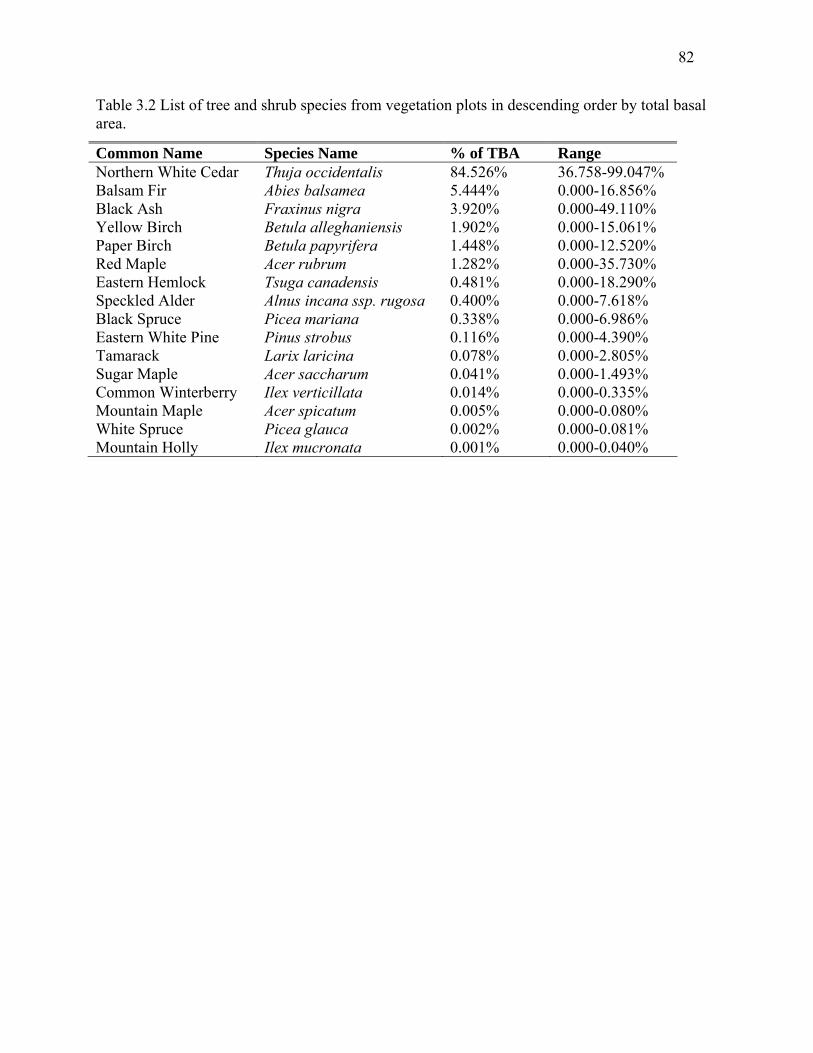
82

Table 3.2 List of tree and shrub species from vegetation plots in descending order by total basal area. Common Name Species Name % of TBA Range Northern White Cedar Thuja occidentalis 84.526% 36.758-99.047% Balsam Fir Abies balsamea 5.444% 0.000-16.856% Black Ash Fraxinus nigra 3.920% 0.000-49.110% Yellow Birch Betula alleghaniensis 1.902% 0.000-15.061% Paper Birch Betula papyrifera 1.448% 0.000-12.520% Red Maple Acer rubrum 1.282% 0.000-35.730% Eastern Hemlock Tsuga canadensis 0.481% 0.000-18.290% Speckled Alder Alnus incana ssp. rugosa 0.400% 0.000-7.618% Black Spruce Picea mariana 0.338% 0.000-6.986% Eastern White Pine Pinus strobus 0.116% 0.000-4.390% Tamarack Larix laricina 0.078% 0.000-2.805% Sugar Maple Acer saccharum 0.041% 0.000-1.493% Common Winterberry Ilex verticillata 0.014% 0.000-0.335% Mountain Maple Acer spicatum 0.005% 0.000-0.080% White Spruce Picea glauca 0.002% 0.000-0.081% Mountain Holly Ilex mucronata 0.001% 0.000-0.040%

83

Table 3.3 Spearman rank correlation (ρ) values and associated P-values for woody stem density across five size classes. Demographic inertia represents the correlation between the density of individuals in each size class and the density of individuals in the preceding size class. Calculation of the weighted wolf occupancy duration index (WWODI) is described in the text. Values in bold with asterisks are considered significant. P-values are Gaussian approximations. With Bonferroni corrections significant p-values are reduced from 0.05 to 0.00167 (α/30). Size Class Canopy Cover Demographic Inertia WWODI A) Density of all woody stem species 1 (10-50cm) ρ = -0.559*, p < 0.0005 ρ = 0.404*, p < 0.05 2 (50-100cm) ρ = -0.107, p = 0.523 ρ = 0.496*, p < 0.005 ρ = 0.602*, p < 0.0001 3 (100-137cm) ρ = -0.221, p = 0.182 ρ = 0.776*, p < 0.0001 ρ = 0.354*, p < 0.05 4 (0-1cm dbh) ρ = -0.213, p = 0.199 ρ = 0.793*, p < 0.0001 ρ = 0.156, p = 0.348 5 (1-2.5cm dbh) ρ = -0.198, p = 0.233 ρ = 0.760*, p < 0.0001 ρ = 0.009, p = 0.955 B) Density of woody stem species likely to exhibit recruitment failure with high browsing pressure: yellow birch, red oak, hemlock, cedar 1 (10-50cm) ρ = -0.416*, p < 0.01 ρ = 0.230, p = 0.164 2 (50-100cm) ρ = -0.089, p = 0.597 ρ = 0.416*, p <0.01 ρ = 0.353*, p < 0.05 3 (100-137cm) ρ = 0.005, p = 0.976 ρ = 0.555*, p < 0.0005 ρ = 0.150, p = 0.367 4 (0-1cm dbh) ρ = 0.142, p = 0.394 ρ = 0.159, p = 0.340 ρ = 0.334*, p < 0.05 5 (1-2.5cm dbh) ρ = -0.021, p = 0.900 ρ = 0.356*, p < 0.05 ρ = 0.084, p = 0.618 C) Density of woody stem species experiencing a competitive advantage from

browsing pressure: balsam fir, speckled alder and spruce 1 (10-50cm) ρ = -0.584*, p < 0.0001 ρ = 0.113, p = 0.499 2 (50-100cm) ρ = -0.391*, p < 0.05 ρ = 0.751*, p < 0.0001 ρ = 0.171, p = 0.305 3 (100-137cm) ρ = -0.610*, p < 0.0001 ρ = 0.773*, p < 0.0001 ρ = 0.143, p = 0.390 4 (0-1cm dbh) ρ = -0.567*, p < 0.0005 ρ = 0.763*, p < 0.0001 ρ = 0.003, p = 0.988 5 (1-2.5cm dbh) ρ = -0.382*, p < 0.05 ρ = 0.659*, p < 0.0001 ρ = -0.006, p = 0.972 D) Density of woody stem species moderately impacted by deer browsing 1 (10-50cm) ρ = -0.489*, p < 0.005 ρ = 0.459*, p < 0.005 2 (50-100cm) ρ = 0.060, p = 0.720 ρ = 0.421*, p <0.01 ρ = 0.635*, p < 0.0001 3 (100-137cm) ρ = 0.292, p = 0.076 ρ = 0.626*, p < 0.0001 ρ = 0.425*, p < 0.01 4 (0-1cm dbh) ρ = 0.195, p = 0.241 ρ = 0.738*, p < 0.0001 ρ = 0.256, p = 0.121 5 (1-2.5cm dbh) ρ = 0.386*, p < 0.05 ρ = 0.750*, p < 0.0001 ρ = -0.005, p = 0.974 E) Density of woody stems of shrub species (not including speckled alder) 1 (10-50cm) ρ = -0.643*, p < 0.0001 ρ = 0.319*, p = 0.05 2 (50-100cm) ρ = 0.039, p = 0.815 ρ = 0.250, p = 0.129 ρ =0.626*, p < 0.0001 3 (100-137cm) ρ = 0.312, p = 0.057 ρ = 0.452*, p < 0.005 ρ =0.238, p = 0.150 4 (0-1cm dbh) ρ = 0.204, p = 0.219 ρ = 0.752*, p < 0.0001 ρ = 0.093, p = 0.579 5 (1-2.5cm dbh) ρ = 0.263, p = 0.111 ρ = 0.694*, p < 0.0001 ρ = -0.138, p = 0.408 F) Density of woody stems of tree species (not including balsam fir or spruce) 1 (10-50cm) ρ = -0.078, p = 0.643 ρ = 0.321*, p < 0.05 2 (50-100cm) ρ = 0.081, p = 0.627 ρ = 0.765*, p < 0.0001 ρ = 0.415*, p < 0.01 3 (100-137cm) ρ = 0.071, p = 0.670 ρ = 0.759*, p < 0.0001 ρ = 0.325*, p < 0.05 4 (0-1cm dbh) ρ = 0.280, p = 0.089 ρ = 0.668*, p < 0.0001 ρ = 0.337*, p < 0.05 5 (1-2.5cm dbh) ρ = 0.439*, p < 0.01 ρ = 0.718*, p < 0.0001 ρ = 0.251, p = 0.129

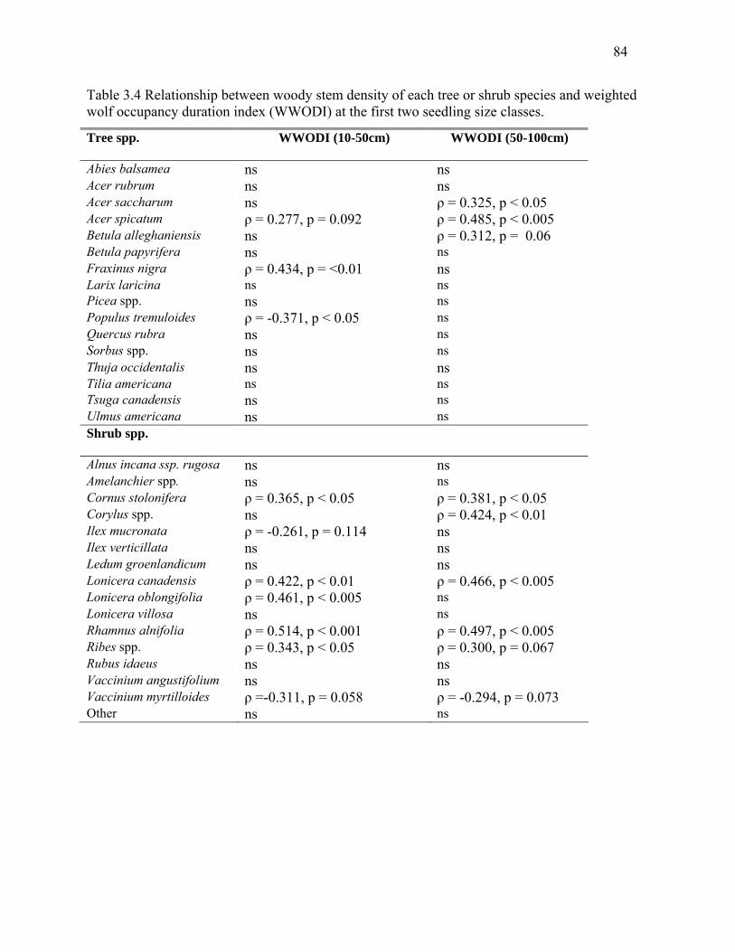
84

Table 3.4 Relationship between woody stem density of each tree or shrub species and weighted wolf occupancy duration index (WWODI) at the first two seedling size classes. Tree spp.

WWODI (10-50cm) WWODI (50-100cm)

Abies balsamea ns ns Acer rubrum ns ns Acer saccharum ns ρ = 0.325, p < 0.05 Acer spicatum ρ = 0.277, p = 0.092 ρ = 0.485, p < 0.005 Betula alleghaniensis ns ρ = 0.312, p = 0.06 Betula papyrifera ns ns Fraxinus nigra ρ = 0.434, p = <0.01 ns Larix laricina ns ns Picea spp. ns ns Populus tremuloides ρ = -0.371, p < 0.05 ns Quercus rubra ns ns Sorbus spp. ns ns Thuja occidentalis ns ns Tilia americana ns ns Tsuga canadensis ns ns Ulmus americana ns ns Shrub spp.

Alnus incana ssp. rugosa ns ns Amelanchier spp. ns ns Cornus stolonifera ρ = 0.365, p < 0.05 ρ = 0.381, p < 0.05 Corylus spp. ns ρ = 0.424, p < 0.01 Ilex mucronata ρ = -0.261, p = 0.114 ns Ilex verticillata ns ns Ledum groenlandicum ns ns Lonicera canadensis ρ = 0.422, p < 0.01 ρ = 0.466, p < 0.005 Lonicera oblongifolia ρ = 0.461, p < 0.005 ns Lonicera villosa ns ns Rhamnus alnifolia ρ = 0.514, p < 0.001 ρ = 0.497, p < 0.005 Ribes spp. ρ = 0.343, p < 0.05 ρ = 0.300, p = 0.067 Rubus idaeus ns ns Vaccinium angustifolium ns ns Vaccinium myrtilloides ρ =-0.311, p = 0.058 ρ = -0.294, p = 0.073 Other ns ns

85

Table 3.5 Spearman rank correlation (ρ) values and associated P-values between weighted wolf occupancy duration index (WWODI) and six commonly used measures of browse intensity. Values in bold with asterisks are considered significant. Index WWODI Deer density DMU -1 n = 38, ρ = -0.019, p = 0.909 Red Maple Browse Index n = 12, ρ = -0.197, p = 0.540 Deer visitation day -1 n = 7, ρ = -0.270, p = 0.558 Bluebead lily (Clintonia borealis) scape height n = 10, ρ = 0.378, p = 0.279 Wild sarsaparilla (Aralia nudicaulis) ha-1 n = 38, ρ = 0.462*, p < 0.005 Nodding trillium (Trillium cernuum) ha-1 n = 38, ρ = 0.479*, p < 0.005

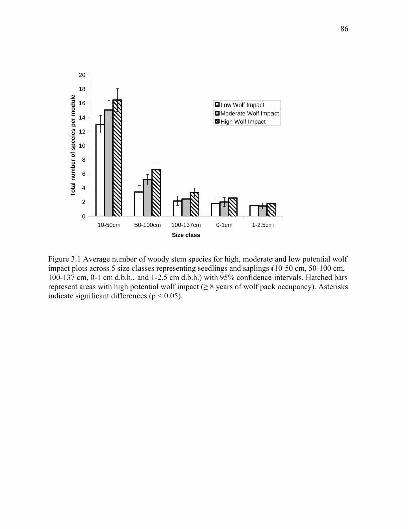
86

0

2

4

6

8

10

12

14

16

18

20

10-50cm 50-100cm 100-137cm 0-1cm 1-2.5cm

Size class

Tota

l num

ber o

f spe

cies

per

mod

ule

Low Wolf ImpactModerate Wolf ImpactHigh Wolf Impact

Figure 3.1 Average number of woody stem species for high, moderate and low potential wolf impact plots across 5 size classes representing seedlings and saplings (10-50 cm, 50-100 cm, 100-137 cm, 0-1 cm d.b.h., and 1-2.5 cm d.b.h.) with 95% confidence intervals. Hatched bars represent areas with high potential wolf impact (≥ 8 years of wolf pack occupancy). Asterisks indicate significant differences (p < 0.05).

87

0

0.5

1

1.5

2

2.5

0 2 4 6 8 10

Weighted wolf occupancy duration index (WWODI)

Shan

non'

s D

iver

sity

Inde

x

Figure 3.2 Linear relationship (y = 0.0934x + 0.798, r2 = 0.379, p<0.0001) between weighted wolf occupancy index values and combined species diversity of shrubs and trees 50-100cm in height at the 100m2 scale. Wolf occupancy values were weighted to give more strength to recent territory extents (see text).

88

0 2 4 6 8 100

200

400

600

WWODI

Trill

ium

cer

nuum

ha

-1

0 2 4 6 8 100

2000

4000

6000

WWODI

Ara

lia n

udic

aulis

ha

-1

0 2 4 6 8 1018

20

22

24

26

28

WWODI

C. b

orea

lis s

cape

hei

ght (

cm)

0 2 4 6 8 100

10

20

30

40

WWODI

Dee

r D

ensi

ty D

MU

-1

0 2 4 6 8 100.6

0.7

0.8

0.9

1.0

WWODI

Red

Map

le B

row

se In

dex

0 2 4 6 8 100.00

0.05

0.10

0.15

0.20

0.25

WWODI

Dee

r Vi

stat

ion

day

-1

Figure 3.3 Relationships between various potential measures of browsing pressure and the Weighted Wolf Occupancy Duration Index (WWODI). Given a trophic cascade response, variables on the left (a-c) were hypothesized to have a positive relationship with WWODI, while variables on the right (d-f) were hypothesized to have a negative relationship with WWODI.

b) e)

c) f)

a) d)

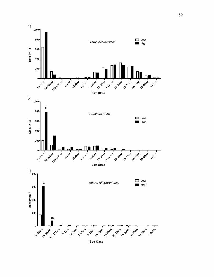
89

10-50

cm

50-10

0cm

100-1

37cm

0-1cm

1-2.5c

m

2.5-5c

m

5-10c

m

10-15

cm

15-20

cm

20-25

cm

25-30

cm

30-35

cm

35-40

cm>4

0cm

0

200

400

600

800

1000

LowHighThuja occidentalis

Size Class

Den

sity

ha-1

10-50

cm

50-10

0cm

100-1

37cm

0-1cm

1-2.5c

m

2.5-5c

m

5-10c

m

10-15

cm

15-20

cm

20-25

cm

25-30

cm

30-35

cm

35-40

cm>4

0cm

0

200

400

600

800

1000

LowHigh

Fraxinus nigra

Size Class

Dens

ity h

a-1

10-50

cm

50-10

0cm

100-1

37cm

0-1cm

1-2.5c

m

2.5-5c

m5-1

0cm

10-15

cm

15-20

cm

20-25

cm

25-30

cm

30-35

cm

35-40

cm>4

0cm

0

200

400

600

800

LowHighBetula alleghaniensis

Size Class

Den

sity

ha

-1

a)

b)

c)

*

*

*

90

10-50

cm

50-10

0cm

100-1

37cm

0-1cm

1-2.5c

m

2.5-5c

m

5-10c

m

10-15

cm

15-20

cm

20-25

cm

25-30

cm

30-35

cm

35-40

cm>4

0cm

0

200

400

600

800

1000

LowHighAbies balsamea

Size Class

Dens

ity h

a-1

10-50

cm

50-10

0cm

100-1

37cm

0-1cm

1-2.5c

m

2.5-5c

m

5-10c

m

10-15

cm

15-20

cm

20-25

cm

25-30

cm

30-35

cm

35-40

cm>4

0cm

0

20

40

60

80

100

LowHigh

Picea mariana

Size Class

Dens

ity h

a-1

Figure 3.4 Distribution of tree density across all size classes for five canopy species of northern white-cedar wetlands. Low impact wolf sites (n=16) represent areas occupied by wolf packs for 0-3 years and are shown with open bars. High impact wolf sites (n=16) represent areas occupied by wolf packs for at least 8-10 years and are displayed with filled bars. Asterisks indicate significant differences (p ≤ 0.05).

d)

e)

91

CHAPTER 4

IS WOLF PACK TENURE AN IMPORTANT VARIABLE WHEN MODELING THE

SPECIES RICHNESS OF CHRONICALLY BROWSED UNDERSTORY PLANT

COMMUNITIES?3


Ecological Applications spring 2011

92

4.0 Abstract:

Wolf (Canis lupus) recovery in the Great Lakes region is anticipated to generate a top-

down trophic cascade by altering white-tailed deer (Odocoileus virginianus) density, habitat

selection, and foraging behavior. Through these direct impacts on white-tailed deer, wolves are

predicted to trigger additional indirect impacts on plant communities chronically browsed by

white-tailed deer. We conducted vegetation surveys in northern white cedar wetlands to measure

species richness of understory plant communities across a gradient of wolf impact. We then

tested three possible hypotheses for observed relationships between species richness and wolf

impact: (1) a top-down trophic cascade, (2) a bottom-up trophic cascade, and (3) a non-trophic

association.

We first calculated a weighted wolf occupancy duration index (WWODI) based on

territory mapping data of known wolf packs from 1995-2009. Using local and regional variables,

we created multivariate models of species richness of forbs (S forbs), shrubs (S shrubs), seedlings (S

seedlings) and ferns (S ferns). We selected the best fit model for each of these vegetation response

variables and examined whether inclusion of WWODI improved model fit, thus distinguishing

bottom-up from top-down trophic effects. To assess the potential for a non-trophic association

we used landscape level variables shown to impact wolf habitat selection to model WWODI.

Again we selected the best fit model and tested whether this model of WWODI was able to

explain any variability in understory plant species richness (S forbs, S shrubs, S seedlings, and S ferns).

In this way we sought to account for spurious associations generated by landscape level factors

known to benefit both plant diversity and wolf habitat quality, irrespective of a trophic effect.

After accounting for local and landscape level environmental factors (such as litter depth,

distance to road, wetness, solar radiation, canopy species richness, precipitation, human

93

disturbance, mean patch area and proximity of similar patches), WWODI still increased the

variability explained by each vegetation response model by 19.0% for S forbs, 10.7% for S shrubs,

and 12.2% for S seedlings, but only by 0.5% for S ferns (based on R2adj values). This suggests that

the positive relationship between WWODI and species richness of forbs, shrubs and seedlings is

unlikely to be a result of bottom-up effects propagating up through the food web.

The best fit landscape model of WWODI included the variables mean patch area (forest)

and mean distance to paved road (R2adj= 46.6%, p<0.001). When these variables were used to fit

species richness data, the models performed poorly, explaining only 3.8% of variability in S forbs,

2.7% of variability in S shrubs, 0.9% of variability in S seedlings, and 3.3% of variability in S ferns

(based on R2adj values). These results suggest that a non-trophic association is an unlikely

explanation for the strong positive relationship between WWODI and S forbs, S shrubs, and S

seedlings.

Duration of wolf pack occupancy was a significant predictor of species richness of

understory plant species known to respond positively to release from herbivory: forbs, shrubs

and seedlings. In contrast, inclusion of WWODI was not supported for models of fern species

richness, a plant group unlikely to respond positively to release from herbivory. These results are

consistent with a top-down trophic cascade triggering a release from browsing pressure by white-

tailed deer in northern white cedar wetlands.

Key Words: trophic cascade, deer browsing intensity, wolf recovery, seedling recruitment, Wisconsin, local and regional variables, AICc, understory plant communities, species richness

94

4.1. Introduction The gray wolf (Canis lupus) is considered a strongly interactive species due to its direct

and indirect effects on lower trophic levels (Soulé et al. 2003). Recovery of the gray wolf in the

Great Lakes region is thus predicted to generate top-down effects that will contribute to the

conservation of regional biodiversity (McShea 2005, Ray 2005). Similar impacts were predicted

of wolf recovery in western North America, and documented changes to those ecosystems have

exceeded expectations (Ripple et al. 2001, Wilmers et al. 2003, Hebblewhite et al. 2005). Has

wolf recovery in the Great Lakes region produced an equally powerful effect?

Several notable characteristics serve to differentiate the ecological role of wolves in the

Great Lakes region, making application of findings from western North America purely

speculative (Rooney and Anderson 2009). For example, successful reintroduction of wolves to

Yellowstone National Park (YNP) corresponded to a 50% decline in elk (Cervus elaphus)

density (White and Garrot 2005, Vucetich et al. 2005), however, the main prey species of wolves

in the Great Lakes region is white-tailed deer (Odocoileus virginianus), and the numerical effect

of wolves on white-tailed deer populations is less clear (Nelson and Mech 1986, Messier 1991,

Nelson and Mech 2006). Ecosystem recovery in YNP occurred primarily in riparian areas, where

high quality elk browse is concentrated (Ripple et al. 2001, Ripple and Bescheta 2003, 2006,

2007, Beyer et al. 2007). In contrast, white-tailed deer forage (forbs and woody plants) is more

evenly distributed throughout the landscape, and deer density is related to distance from northern

white cedar (Thuja occidentalis) wetlands which provide important winter habitat (Millington et

al. 2010).

The Great Lakes Region has fewer predator and ungulate species than YNP indicative of

a less complex food web (Smith et al. 2003, Kurta 1995), and represents a simplification of the

95

original ecosystems and more diverse ungulate populations that existed in the Great Lakes region

prior to European settlement (DelGiudice et al. 2009). Food web complexity has been argued to

dampen the indirect effects of trophic cascades (Halaj and Wise 2001), so recovery of wolves in

the Great Lakes region may in fact generate stronger impacts on lower trophic levels than those

observed in YNP. However, western riparian areas are subject to intense disturbance regimes and

show great resilience to disturbance (White and Stromberg in press). Understory plant

communities of the Midwest experience much lower disturbance intensity and are likely to

demonstrate ecological hysteresis (Cote et al. 2004). Diversity of plant communities also plays

an important role in ecosystem resilience by contributing to the variety of responses to

environmental change (‘response diversity’ sensu Elmqvist et al. 2003). Finally, human density

and road density are both considerably higher in the Great Lakes region and are known to

influence wolf habitat selection (Mladenoff et al. 1995), white-tailed deer forage availability

(Rooney and Anderson 2009), and understory plant diversity (Findlay and Houlahan 1997,

Watkins et al. 2003).

The hyper-abundance of white-tailed deer in the Great Lakes region suggests that trait

mediated indirect effects may be a more likely mechanism than density mediated direct effects in

altering browsing pressure on understory plant communities. The reintroduction of wolves to

YNP has shown that foraging prey species alter their spatial use of available habitat in the

presence of top predators (Ripple et al. 2001, Ripple and Beschta 2003). Ungulates in YNP were

also observed to reduce the total amount of time allocated to foraging activities due to increased

vigilance (Lima and Dill 1990, Laundré et al. 2001). Unfortunately, these behavioral prey

responses have not been well documented in the Great Lakes region.

96

Given these caveats, where should we begin to look for a top-down trophic response to

recovery of gray wolves in the Great Lakes region? What response variables should we measure?

How can we detect the signal of a top-down trophic response above the ambient noise of

ecological variation? Previous research by Anderson et al. (unpublished data) showed that the

biomass of forb and woody-browse species in northern white cedar wetlands increased toward

the center of wolf pack territories. A similar pattern was not observed in other forest-cover types

(coniferous forest, deciduous forest and mixed forest), leading Anderson et al. to conclude that

trophic cascades in this region are more detectable in browse-sensitive communities with low

productivity and high species richness (i.e. cedar wetlands).

Due to differences in life history traits, such as longevity, reproductive rate, dispersal

ability and resource allocation to physical and chemical defenses, plant species differ drastically

in their response to herbivory. Documented changes over the past 50 years in upland forest

stands of northern Wisconsin show an average decline of 18% in the species richness of

understory plant communities (Rooney et al. 2004). Species in decline were those known to be

sensitive to deer browsing such as palatable forbs and tree seedlings. In contrast, ferns and

grasses (generally considered to be either resistant or tolerant of deer browsing) appear to be out-

competing more sensitive species (Weigmann and Waller 2006). Thus, we anticipated that

understory plants would vary in their response to release from browsing pressure dependent on

the vegetation growth form in question (forbs, shrubs, seedlings or ferns). On the Alleghany

Plateau, Horsley et al. (2003) found a negative relationship between species richness of seedlings

and deer density and a positive relationship between percent cover of ferns and deer density.

Based on the concept that species diversity is maximized when disturbance conditions match the

historic disturbance regimes under which plant communities developed (Denslow 1985)

97

combined with trophic cascade theory (Schmitz 2006), we hypothesize that species richness of

forb, shrub, and seedling species should be higher at high wolf impact areas (since deer browsing

pressure should be reduced and closer to historic levels).

The pattern of wolf recolonization has produced a chronosequence of wolf impact across

the landscapes of Minnesota, Wisconsin and Michigan. The Wisconsin Department of Natural

Resources (WiDNR) has annually mapped wolf pack territory extents since 1979. The high

quality of this dataset provides the information needed to explicitly examine the spatial and

temporal pattern of wolf occupancy throughout the state (Wiedenhoeft and Wydeven 2005).

Some areas have been occupied by wolf packs for more than 15 years, some areas were never

successfully recolonized by wolves, and many areas exhibit wolf occupancy duration

intermediate between these two extremes. This gradient provides a natural experimental

framework with which to measure vegetation response as a function of time since wolf

colonization (Rooney and Anderson 2009).

The danger in space-for-time studies is the potential for confounding variables to produce

spurious associations. Several factors benefit both plant diversity and wolf habitat quality,

irrespective of deer density and any sort of trophic effect. In particular, road density has been

shown to be negatively correlated with both plant diversity (Findlay and Houlahan 1997, Rogers

et al. 2009) and wolf habitat selection (Mladenoff et al. 1995). Understory vegetation in white

cedar stands may also be more influenced by hydrology (drainage rate and variability in depth to

water table) and edge effects than by variation in browsing pressure. A bottom-up effect could

also result in a positive relationship between plant species richness and wolf impact: areas with

high plant biomass and diversity could maintain higher deer densities which in turn support

successful wolf pack establishment.

98

Our objective was to determine the relative importance of wolf occupancy duration in

predicting the species richness of understory plant communities of northern white-cedar

wetlands. We further sought to rule out potentially confounding factors and to distinguish top-

down from bottom-up trophic effects. Our approach was three fold. We first created univariate

models of species richness based solely on wolf occupancy duration (top-down model). Second,

we modeled species richness of forbs, shrubs, seedlings and ferns based on both local and

landscape level variables known to be associated with plant species richness (bottom-up model).

We then added wolf occupancy duration to these models to see if the addition of WWODI as a

predictor variable improved model accuracy. Our third approach was to model wolf occupancy

duration itself based on landscape variables known to influence both wolf habitat selection and

plant species richness (non-trophic model). We then tested the accuracy of this model in

predicting species richness of plants. Effects attributed to wolf impact based on the top-down

model of plant species richness not accounted for by the bottom-up or non-trophic model are

thus hypothesized to represent pure top-down trophic effects. This remaining proportion of

variability in plant species richness is likely due to release of understory plant communities from

over-browsing by white-tailed deer responding to the local establishment and consistent

occupancy of wolf pack territories.

4.2. Methods

4.2.1 STUDY SITE


various state and county forests spanning 7 counties in north-central Wisconsin. The forests of

Northern Wisconsin are transitional between deciduous forests to the south and boreal forests to

99

the north (Pastor and Mladenoff 1992, Mladenoff et al. 1993). Annual air temperature in

northern Wisconsin averages 4º C, and mean annual precipitation ranges between 76 and 86 cm.

The freeze free period averages ~80 days, making for a short growing season. Snowfall

accumulation frequently exceeds 76 cm and the snow cover provides insulation for ground

vegetation (NOAA 1982).

Glaciation strongly influenced the soils and topography of Wisconsin. Soils are derived

from sandy loam glacial till, silt covered glacial tills, and sandy outwash. With a maximum

elevation of 550 m, there is little topographic relief. The gently rolling terrain is inundated with

thousands of lakes and numerous wetlands. Terrestrial landscapes are comprised of 40%

deciduous forest types (dominated by sugar maple, Acer saccharum and paper birch, Betula

papyrifera), 9% coniferous, (dominated by white pine, Pinus resinosa, red pine, Pinus strobus,

and balsam fir, Abies balsamea), 8% mixed-coniferous-deciduous, and 7% early successional

(dominated by aspen, Populus tremuloides). Forested and emergent wetland communities cover

an additional 26% of the area (dominated by tamarack, Larix laricina and black spruce, Picea

mariana, and Labrador-tea, Ledum groenlandicum and leather leaf Chamaedaphne calyculata,

respectively). Northern-white cedar wetlands occupy less than 5% of the landscape but support a

large proportion of the regional biodiversity (WiDNR 1998).

Northern-white cedar wetlands develop on poorly-drained sites with a slight through-flow

of groundwater. These conditions elevate the pH and nutrient richness of the soil (Black and

Judziewicz 2008). Mature stands of white cedar are densely shaded with nearly closed canopies.

The combination of these environmental characteristics produces unique light regimes and soil

chemistry required by species restricted to this community type. Co-dominant trees in white

cedar wetlands include balsam fir, yellow birch (Betula alleghaniensis) and black ash (Fraxinus

100

nigra). Speckled alder (Alnus incana subsp. rugosa), hollies (Ilex mucronata and I. verticillata),

hazelnuts (Corylus spps.) and honeysuckles (Lonicera spps.) are common understory shrubs.

Cedar wetlands are also rich in wildflowers ranging from the common to the extremely

rare. Common wildflowers are goldthread (Coptis trifolia), starflower (Trientalis borealis), wild

sarsaparilla (Aralia nudicaulis), naked miterwort (Mitella nuda), blue-bead lily (Clintonia

borealis), bunchberry (Cornus canadensis), Canada mayflower (Maianthemum canadense), and

trailing “sub-shrubs” such as creeping snowberry (Gaultheria hispidula), dwarf red raspberry

(Rubus pubescens) and twinflower (Linnea borealis). Orchids include yellow lady’s slipper

(Cypripedium parviflorum), heart-leaved twayeblade (Listera cordata), lesser rattlesnake

plantain (Goodyera repens), and blunt-leaved bog orchid (Platanthera obtusata).

Fern species found in northern white cedar stands include cinnamon fern (Osmunda

claytoniana), American royal fern (Osmunda regalis var. spectabilis), interrupted fern (Osmunda

claytoniana), wood ferns (Dryopteris spps.), lady fern (Athyrium filix-femina var. angustum),

common oak fern (Gymnocarpium dryopteris), sensitive fern (Onoclea sensibilis), narrow beech

fern (Phegopteris connectilis), rattlesnake fern (Botrychium virginianum) and occasionally

bracken fern (Pteridium aquilinum var. latiusculum). See appendix A for a complete species list.

Wolves have been recolonizing northern Wisconsin since the early 1970s, but wolf

distribution remained very limited until the 1990s (Wydeven et al. 1995, Wydeven et al. 2009).

Depending on pack size and prey density, wolf territories in the Great Lakes Region can range in

size but recently averaged approximately 136 km2 (Wydeven et al. 2009). Hoskinson and Mech

(1976) reported that deer survival is higher on the edges of wolf territories as compared to their

centers. Wolves are less likely to hunt in these buffer zones so as to avoid potentially fatal


101




In the Great Lakes region, deer winter home ranges vary between 730 and

1859 ha (Van Deelen et al. 1998). Early studies in Wisconsin indicated that mature white-tailed

deer consume between two and nine kilograms of quality browse per deer per day (Taylor 1956).

Predator extirpation, when combined with protective hunting laws and habitat management, has

contributed to current deer densities ranging between 4 and 15/km2 (Wi DNR 2008). Alverson et

al. (1988) prescribed densities as low as 1-2 deer/km2 to improve recruitment of sensitive plant

species.

Wolves require 15-18 deer ‘equivalents’ per wolf per year (Fuller 1995). Hence the

current Wisconsin wolf population, which has grown to ~690 individuals (Wydeven and

Wiedenhoeft 2010), has the capacity to take ~12,000 deer per year. Given that there are an

estimated 390,000 deer in the Northern Forests of Wisconsin (posthunt), region-wide effects of

wolf recovery on deer populations are unlikely to manifest in the short term (Pers. comm. Keith

McCaffery 2008). In addition, whether wolf kills represent primarily compensatory or additive

mortality for white-tailed deer is in part dependent on stochastic environmental variables (Mech

and Peterson 2003). However, localized influences on deer populations are more probable, and

drastic local reductions have been observed in Minnesota (Nelson and Mech 2006).

4.2.2 DATA COLLECTION

WiDNR population estimates of wolves were ascertained by live-trapping and radio

tracking (Mech 1974, Fuller and Snow 1988), howl surveys (Harrington and Mech 1982), and

102

winter track surveys (Thiel and Welch 1981, Wydeven et al. 1995). Territory extents are

delineated using minimum convex polygons based on radiolocations of collared wolves and

other wolf sign (Wydeven et al. 1995). Using ArcGIS 9.3, we overlaid current wolf territories

with historic territory extents back to 1995. Only sites within the Chequamegon-Nicolet National

Forest or state and county forest boundaries were selected. Although wolves have established

territories outside of public lands, these territories are often located in agricultural or industrial

forest landscapes and anthropogenic sources of landscape change are likely to obscure any

potential trophic effects of wolf recolonization.

White-tailed deer density data (WiDNR 2009) was obtained for each deer management

unit (DMU) for the 15 years prior to vegetation data collection. WiDNR calculates initial deer

density estimates using the sex-age-kill method and then corrects for the proportion of the DMU

that is considered deer habitat (Millspaugh et al. 2006). Wisconsin DMUs are vastly larger in

area than the cedar stands and wolf pack territories they contain. Since a deer density estimate

for a given DMU is a single value intended to represent an average across a very large

heterogeneous area, it is unlikely that these values represent the site specific deer density

influencing the understory of isolated cedar stands. However, this was the only historical data

available for our entire study area.


Forest (USDA 2001) and various state and county forest datasets to select stands characterized as

northern white cedar wetlands. Hawth’s Analysis Tools add-on for ArcGIS (Beyer 2004) was

used to randomly place one vegetation plot within each pre-selected white cedar stand. We

surveyed a total of 38 cedar stands across a gradient of wolf impact. Fourteen plots were

completed in 2008 and 24 plots were completed in 2009. Vegetation surveys followed the

103

Carolina Vegetation Survey (CVS) protocol developed by Peet et al. (1998). Plots consisted of 4

modules (10 X 10 meters) in a 2 X 2 configuration. Two corners in each module were sampled

for presence of vascular plant species (trees, shrubs, seedlings, ferns, forbs) using a series of

nested quadrats (increasing incrementally in size from 0.01 m2 to 10 m2).

Species richness of forbs, shrubs and ferns was determined for the 10 m2 scale for each of

eight subsamples and then averaged to produce a single richness estimate for each vegetation

plot (n=38). Understory seedling species richness was determined by averaging species richness

at the 100m2 scale based on only two subsamples per plot (two 10 X 10 m modules per plot).

Identification of forbs conforms to Black and Judziewicz (2008), other plant species names

conform to Gleason and Cronquist (1991).

4.2.3 WEIGHTED WOLF OCCUPANCY DURATION INDEX AND DEER DENSITY

Wolf packs establish and occupy territories that are patchily distributed across the

landscape (Mladenoff et al. 1999). The effect of wolves on deer abundance and foraging

behavior is likely to be limited to locations continuously occupied by wolf packs. Presumably,

the impact of wolves increases with the number of years the territory has been consistently

occupied. Since pack size and territory extent vary from year to year, this creates a mosaic of

potential impact intensity across the landscape.

Weighted wolf occupancy duration Index (WWODI) values were calculated by summing

the most recent 15 years of DNR wolf territory extent data (1993-2007 for vegetation plots

surveyed in 2008 and 1994-2008 for plots surveyed in 2009). Recent years were weighted more

strongly given the assumption that wolf occupancy in the distant past would have a weaker

impact on current browse intensity and therefore a weaker indirect effect on understory plant

104

communities. The most recent year of wolf occupancy (presence/absence of a wolf pack at each

location) was divided by 1, the next most recent year was divided by 1.1, and so on. Thus:

WWODI = Yt/1+ Yt-1/1.1 + Yt-2/1.2 + ……..Yt-15/2.4

where Yt is the current year of wolf occupancy and Yt-15 is the wolf occupancy 15 years ago.

Although we had hoped to calculate wolf density by dividing territory area by the number of

wolves in each pack, pack size data was not consistently collected for all years and all packs.

A similar process was used to calculate a 15 year weighted index for deer density DMU-1.

To calculate the 15 year weighted index for deer density, we divided the current year by one, the

next most recent year by 1.1, then by 1.2 and so on until 15 years before data collection. Again,

these values were summed to provide a weighted index of deer density.

4.2.4 LOCAL AND LANDSCAPE VARIABLES

Remnant northern white cedar stands are often embedded within an early successional

forest matrix representing isolated islands of speciose plant communities (Cornett et al. 2000).

Cedar wetlands of various shapes and sizes are patchily distributed throughout the landscape. In

such a patchy environment, species establishment of forbs and shrubs will depend on their ability

to disperse into the stand and persist long enough to successfully reproduce. Assuming that our

focal wetlands are drawing from the same regional species pool, species richness represents the

outcome of the combined suite of restraints influencing both dispersal and persistence. Dispersal

is determined by landscape level variables influenced by the configuration of habitat types and

level of fragmentation. Persistence is determined by local biotic and abiotic factors. Biotic

factors impacting understory plant survival are competition with other plant species, seed

105

predators, pathogens, symbiotic relationships with mycorrhizae, and herbivory by white-tailed

deer.

Local environmental factors shown to influence plant survival and reproductive success

(Table 4.1a) are canopy cover (Brosofske et al. 1999), litter depth (Xiong and Nilsson 1999),

slope (Honnay et al. 1999, Kumar et al. 2006, Marini et al. 2008), elevation (Kumar et al. 2006,

Marini et al. 2008), Canopy S (Brosofske et al. 1999), patch area (Findlay and Houlahan 1996,

Marini et al. 2008, Rogers et al. 2009), patch age (Matthews et al. 2009), wetness (Wright et al.

2003, Matthews et al. 2009), solar radiation (Marini et al. 2008), precipitation (Marini et al.

2008, Matthews et al. 2009), distance to road (Brosofske et al. 1999, Watkins et al. 2003), and

proportion of sand in the soil (Kumar et al. 2006).

We measured canopy cover with a densiometer, averaging readings from the center of

each 100m2 module facing the four cardinal directions. Litter depth was measured to the nearest

centimeter per module. The “Wetness” variable was based on a visual estimate of the percentage

of each module that was covered by standing water. Species richness of canopy trees (Canopy S)

is simply the number of canopy species per module. All variables measured in the field were

averaged across four modules to produce a single value per vegetation plot.

Patch area and patch age were obtained from stand level data from the Chequamegon

Nicolet National Forest CDS data and various state and county datasets. Elevation was acquired

from 30m Digital Elevation Models (DEMs) of the study area. Slope and solar radiation were

derived from the same DEM dataset using the slope and solar radiation tools in ArcGIS 9.2.

Solar radiation represents the cumulative radiation for the month of May, 2009 in kWH/m2

(similar to Marini et al. 2008). Precipitation represents the cumulative precipitation (in mm) for

May, June, July, August, and September, 2008 (similar to Marini et al. 2008) based on data from

106

NOAA (2008). We measured distance to the nearest road (all road types) based on Tiger line

files for Wisconsin roads (US Census Bureau 2000). The proportion of sand in the surficial

deposits layer (which directly affects permeability and drainage rate) was obtained from the

Groundwater Contamination Susceptibility Model (1:500,000 scale) developed by WiDNR et al.

(1997).

Landscape level factors thought to influence dispersal success of understory plant species

(Table 4.1b) are mean patch area (Honnay et al. 2003, Kumar et al. 2006), edge density (Honnay

et al. 2003, Kumar et al. 2006, Marini et al. 2008), proportion of disturbed land (Honnay et al.

2003, Marini et al. 2008, Matthews et al. 2009, Rogers et al. 2009), proportion of forested land

(Honnay et al. 1999, Honnay et al. 2003, Marini et al. 2008, Rogers et al. 2009), proportion of

open water (Matthews et al. 2009), Shannon’s Diversity Index of the landscape (Honnay et al.

2003), paved road density (Findlay and Houlahan 1996, Rogers et al. 2009), proximity of similar

patches (Rogers et al. 2009), and aggregation/interspersion of similar patches (Kumar et al.

2006).

Although most authors use paved road density as a landscape variable, we used mean

distance to paved road. We chose to use the aggregation index because He et al. (2000) found

that this index out performs other measures of juxtaposition/interspersion (contagion index,

shape index, probability of adjacency of the same class) because it is class specific. For

landscape variables requiring a patch type such as total edge density, proximity index and

aggregation index we used a combined patch type we called ‘coniferous forest’. We combined

the GAP Land Cover vegetation types ‘white spruce’ and ‘alkaline conifer’ to represent

‘coniferous forest’ because the algorithm GAP used to assign vegetation classes did not seem to

107

successfully differentiate between these two vegetation types (most of our cedar stands were

categorized as white spruce and should have been categorized as alkaline conifer).

In southeastern Ontario wetlands, Findlay and Houlahan (1997) found the critical

distance in plant species richness response to landscape variables to lie between 1000 and 2000

m. Based on this previous study, we calculated our landscape variables within a 1,000 m buffer

of each vegetation plot using GAP Land Cover data (USGS 2010). We also calculated mean

distance to paved roads within 1000 m buffer using Tiger line files for Wisconsin roads (US

Census Bureau 2000). ArcGIS 9.2 (ESRI) and FRAGSTATS (McGarigal et al. 2002) were used

to extract and summarize the variables. All data were projected using the HARN Wisconsin TM

(NAD 83) coordinate system.

4.2.5 MODEL SELECTION

We used ordinary least squares regression (OLS) to examine relationships between our

predictor and response variables. Variables displaying OLS regression coefficients with p < 0.10

were retained in the global models for each response variable (Millington et al. 2010). Once

global models were formulated, we applied a model-selection approach (Burnham and Anderson

2002) using Akaike’s information criterion (AICc) to determine the best-fitting model from

among the candidate set of models (all possible variable combinations).

We also used model selection to compare our competing hypotheses for explaining

observed relationships between WWODI and S forbs, S shrubs, S seedlings, and S ferns: (1) the top-

down hypothesis, (2) the bottom-up hypothesis, and (3) the non-trophic hypothesis. To evaluate

the evidence in support of a bottom-up trophic cascade, we selected the best models for

predicting species richness of forbs, shrubs, seedlings and ferns, based on local and landscape

108

level factors, and examined whether the addition of wolf impact (WWODI) improved model fit

(similar to Beyer et al. 2007). We also observed the difference in R2 adj values between

competing models with and without WWODI.

To evaluate the evidence in support of the non-trophic association hypothesis, we applied

the best fitting model for WWODI (WWODImodel) to our vegetation response variables (S forbs, S

shrubs, S seedlings, and S ferns ) to determine the amount of variability in species richness explained

by these landscape variables thought to influence both wolf habitat selection and plant species

richness. We further compared model performance using R2 adj values by subtracting the

variability in plant species richness accounted for by landscape level variables associated with

wolf habitat selection (WWODImodel) from the variability initially attributed to top-down effects

(WWODI). All statistical analyses were performed using SAS 9.1 software (Cary, NC, USA).

4.3. Results

4.3.1 UNIVARIATE MODELS

Table 4.2 shows descriptive statistics for the response variables (S forbs, S shrubs, S seedlings,

and S ferns). All vegetation response variables were normally distributed according to Anderson-

Darling normality tests. The weighted wolf occupancy duration index ranged from 0.00 – 9.47

with an average value of 4.66 ± 0.51 (SE). Figure 1 shows linear relationships between WWODI

and the four vegetation response variables (S forbs, S shrubs, S seedlings, and S ferns) (n=38). The

strong positive relationships between WWODI and S forbs (R2 = 30.2%, p< 0.001) and WWODI

and S shrubs (R2 = 21.2%, p< 0.005) are consistent with an indirect trophic response to wolf

recovery (Table 4.3). The relationship between WWODI and S seedlings (R2 = 11.4%, p< 0.05) is

not as strong as expected but still significant and positive. We did not anticipate a positive

109

response of S ferns to release from deer browsing since ferns are generally unpalatable and tend to

display competitive release under high browsing pressure. However, our data suggest a weak and

non-significant but positive relationship between WWODI and S ferns (R2 = 5.3%, p= 0.166).

Current year deer density DMU-1 estimates ranged from 2.64 km-2 to 13.12 km-2 with an

average value of 6.44 ± 0.33 km-2. This variable was unrelated to any of the vegetation response

variables and was not used in further analyses. The fifteen year weighted deer density DMU-1

index ranged from 44.25 to 126.66 with an average value of 71.10 ± 2.45. This variable was also

unrelated to S forbs, S shrubs, S seedlings or S ferns (Table 4.3). Percent cover of ferns showed no

significant relationship with deer density but was negatively related to WWODI (R2 = 11.8%, p

<0.05). Deer density at this scale was unrelated to WWODI (R2 = 0.5%, p = 0.68).

Table 4.4 shows the descriptive statistics for independent local and landscape level

variables used in the model selection process. To avoid multicollinearity, predictor variables with

Pearson correlation coefficients above a threshold of 0.49 were removed (Moore and McCabe

1993). Elevation was highly correlated with wetness (r = -0.625, p < 0.001) and precipitation (r =

-0.739, p < 0.001) and was removed. Proportion of forested land was negatively correlated with

Shannon Diversity Index of the landscape (r = -0.843, p < 0.001) and with the proportion of sand

in the surficial deposits layer (0.650, p < 0.001) and was removed. Aggregation index was

positively correlated with the proximity index (0.510, p < 0.001) and was removed. Cedar stand

area was positively correlated with mean patch area (coniferous forest) (0.537, p < 0.001) and

was removed. Retained variables had stronger relationships with response variables in all cases.

Variables were further reduced by removing those that failed to demonstrate a univariate

relationship with the response variables (variables displaying OLS regression coefficients with p

≥ 0.10). Slope, SDI of the landscape and patch age showed weak or nonexistent relationships

110

with S forbs, S shrubs, S seedlings, S ferns or WWODI and were thus removed from the global models.

Figures 2-6 show the univariate relationships between S forbs, S shrubs, S seedlings, S ferns and their

respective retained independent variables.

4.3.2 MODEL-SELECTION

Variables retained in the global models of each response variable are shown in Table 4.5.

The global model for S forbs consisted of litter depth, percent standing water, distance to road,

proportion disturbed, and proportion open water. The global model for S shrubs consisted of

proportion disturbed, canopy cover and canopy species richness (S). The global model for S

seedlings consisted of mean patch area of forest, canopy species richness (S) and proportion sand.

The global model for S ferns consisted of proximity index (for coniferous forest), solar radiation,

precipitation, and litter depth.

The highest ranking models (based on 95% Akaike weights (wi)) for our vegetation response

variables (S forbs, S shrubs, S seedlings, S ferns) are presented in Table 4.6.

Among the candidate model set, the model with the most support for S forbs indicated that

species richness of forbs is negatively related to litter depth (β = -0.7629 ± 0.3139 [mean ± SE]),

negatively related to proportion disturbed (β = -59.93 ± 18.12), and positively related to wetness

(β = 0.5466 ± 0.2203). The model with the most support for S shrubs indicated that species

richness of shrubs is negatively related to proportion disturbed (β = -13.242 ± 7.847), and

negatively related to canopy S (β = 0.2999 ± 0.1396). The model with the most support for S

seedlings indicated that species richness of seedlings is positively related to canopy S (β = 0.4910 ±

0.2047), and positively related to proportion of sand in the surficial deposits layer (β = 1.6558 ±

0.001719). The model with the most support for S ferns indicated that species richness of ferns is

111

positively related to the proximity index (coniferous forest) (β = 0.003839 ± 0.2047), positively

related to precipitation (β = 0.02390 ± 0.01398) and negatively related to litter depth (β = -

0.2642 ± 0.1317).

4.3.3 EVIDENCE FOR COMPETING HYPOTHESES

We tested three possible hypotheses for observed relationships between species richness

and wolf impact: (1) a top-down trophic cascade, (2) a bottom-up trophic cascade and (3) a non-

trophic association. There was strong support for the top-down trophic cascade model for species

richness of forbs, shrubs and seedlings, but not for ferns (Figure 1 and Table 4.3).

When we took the predictor variables from the best-fit model for each vegetation

response variable and added WWODI to the variables used in the candidate model set (all

possible combinations of variables), models for S forbs, S shrubs, and S seedlings containing WWODI

consistently outperformed models without WWODI (Table 4.7). The top models of S forbs, S

shrubs, and S seedlings (representing 98%, 91% and 86% of Akaike weights, respectively) contained

WWODI as a predictor variable. Models containing WWODI were 264 times, 12 times, and 11

times more likely to be true than the best-fit models without WWODI for S forbs, S shrubs, and S

seedlings, respectively. In contrast, the top models for S ferns did not contain WWODI (representing

42% of Akaike weights) and the original best-fit model containing only local and landscape

variables had 2.3 times more support than the same model with WWODI. The parameter

estimates for the model averaged model for each response variable, when candidate models

included WWODI, are provided in Table 4.8.

After accounting for environmental effects on species richness, WWODI still increased

the variability explained by each model by 19.0% for S forbs, 10.7% for S shrubs, and 12.2% for S

112

seedlings, but only by 0.5% for S ferns (based on R2adj, Table 4.9). This suggests that while local and

landscape level factors have a major impact on plant species richness, the positive relationship

between WWODI and species richness of forbs, shrubs and seedlings is more likely due to a top-

down trophic cascade triggering a release from herbivory than to bottom-up effects propagating

up through the food web.

The best fit landscape model of WWODI (again based on lower AICc values and higher

Akaike weights (wi)) included the variables mean patch area (forest) and mean distance to paved

road (R2adj= 46.6%, p<0.001). When the variables for this WWODI model were used to fit

species richness data it performed poorly, explaining only 3.8% [R2adj] of variability in S forbs,

2.7% of variability in S shrubs, 0.9% of variability in S seedlings, and 3.3% of variability in S ferns

(Table 4.10). Since our best-fit model only accounts for 46.6% of the variability in wolf

occupancy, it is possible that the independent variables responsible for the unexplained variance

in WWODI are more strongly associated with species richness. However, based on the landscape

level variables we assessed, a non-trophic association is an unlikely explanation for the strong

positive relationship between WWODI and S forbs, S shrubs, and S seedlings.

4.4. Discussion

After we accounted for local and landscape factors, the duration of wolf pack occupancy

was a significant predictor of species richness of understory plant species known to respond

positively to release from herbivory: forbs, shrubs and seedlings. In contrast, species richness of

ferns showed a possible weak positive relationship with WWODI, but this relationship was more

likely due to non-trophic associations. In addition, inclusion of WWODI was not supported for

113

models of fern species richness. These results are consistent with a top-down trophic cascade

triggering a release from browsing pressure by white-tailed deer.

Evidence from the Allegheny Plateau, predicts that ferns represent aspects of understory

plant communities that will not respond to release from browsing pressure (Horsley and Marquis

1983), indicative of an alternate stable state (Friedel 1991, Laycock 1991, Stromayer and Warren

1997). While our data do not indicate an effect of wolf occupancy (and by extension release from

browsing pressure) on species richness of ferns, we did find a negative relationship between wolf

occupancy and percent cover of ferns. However, a reduction in percent cover could indicate

either that individual fern plants do not grow as large due to over-shading by shrubs, or that some

fern plants are being out-competed by shrubs which could eventually lead to a decline in local

species richness of ferns.

We found little evidence to support that species richness of understory plant communities

are associated with white-tailed deer density at the scale of deer management units. However, as

stated earlier, deer density estimates representing entire DMUs are unlikely to characterize the

site specific deer density influencing the understory of isolated cedar stands. A better estimate of

local browse pressure is clearly needed (e.g. density of Aralia nudicaulis, see Chapter 3). The

lack of association between deer density DMU-1 and WWODI is not surprising given the

inappropriate scale of the deer density data (most DMUs in our study area had both high and low

wolf impact areas). Given the low density of wolves, however, numerical effects on deer

populations may be unlikely. Our objective was not to model effects of wolves on white-tailed

deer population growth, and a more comprehensive approach is needed to test these assumptions

(see Van Deelen et al. in review). Regardless of numerical effects, the consistent presence of a

wolf pack is predicted to alter: (1) local habitat selection by white tailed deer (i.e. buffer zones

114

between adjacent packs act as refugia), and/or (2) foraging behavior by white-tailed deer (i.e.

deer increase vigilance and movement).

Initial evidence from YNP indicated trait mediated indirect effects of wolves on aspen,

cottonwood and willow recruitment (Ripple et al. 2001, Ripple and Beschta 2003, 2004, 2007,

Beyer et al. 2007). However, several recent studies question the scientific validity of these earlier

works. For example, Creel and Christianson (2009) found that elk consumption of willow

actually increased when wolves were present. They cite eight years of low snow accumulation

(causing elk to reduce browsing in favor of grazing) and declines in elk density as the proximate

causes for willow recovery. When Kaufmann et al. (2010) used an a priori measure of predation

risk based on actual predation events, incorporated abiotic factors, and conducted a multi-year

manipulative experiment, they found no evidence for a behaviorally mediated trophic cascade

(BMTC) triggering recovery of aspen. They argue that the reduction in elk numbers (due at least

in part to wolf predation) will have reduced browsing pressure by ~40%, and that this numerical

effect is responsible for the patchy recovery of aspens, cottonwoods and willows in areas with

high productivity.

Since our abiotic environmental models were only able to explain some of the variability

in species richness of forbs (39.1%), shrubs (19.6%), seedlings (21.3%), and ferns (31.7%), it is

possible that we missed some important factors influencing species richness of understory plant

communities in northern white cedar swamps. For example, several studies have found

significant relationships between species richness and soil properties such as total soil nitrogen,

organic carbon, pH and reduction potential (Kumar et al. 2006, Matthews et al 2009). However,

Weiher et al. (2003) found the total effect of soils on species richness in Wisconsin oak

savannahs to be negligible as the effects of different components canceled each other out (some

115

were positive and some negative). Regardless, it is doubtful that wolf occupancy is correlated

with soil properties, so inclusion of these variables would be unlikely to weaken support for a

top-down trophic effect.

Fawn predation by black bears (Ursus americanus) is considered an important mortality

factor for white-tailed deer, and black bear numbers have been relatively high in Wisconsin in

recent years (Rolley and Worland 2009). Since adult deer are not preyed upon by bears, fawn

predation alone is likely to have relatively weak effects on population growth of white-tailed

deer. However, some evidence suggests that the regional coexistence of wolves and bears may

limit population irruptions of moose (Alces alces) (Gassaway et al. 1992, Messier 1994). Whether

this same pattern will be observed for white-tailed deer in the Great Lakes region is of significant

management interest. The possible synergistic effects of wolf and bear predation may have

exaggerated the variability in plant species richness that we attributed to top-down effects of wolf

recovery.

4.5. Conclusion

Most previous studies of top-down trophic effects of wolves used wolf presence and/or

predation risk by wolves as a dichotomous variable in either space or time (Ripple et al. 2001,

Ripple and Beschta 2003, Ripple and Beschta 2004, Hebblewhite et al. 2005, Ripple and Beschta

2006, Beschta and Ripple 2007, Beyer et al. 2007). Here we provide wolf impact as a gradient

representing the historic spatial extents of wolf pack territories through time since colonization.

Plant species are thought to recover slowly from disturbance (Foster 1992, Pearson et al. 1998),

so current vegetation conditions will reflect historic disturbance patterns, making a gradient in

space and time a more appropriate variable for measuring top-down trophic effects.

116

We also incorporated local and landscape level factors thought to impact our vegetation

response variables and employed model selection using an information theoretic approach.

Through this process, we showed a lack of evidence for competing explanations for the positive

relationship we found between wolf occupancy duration and plant species richness of forbs,

shrubs and seedlings at local scales (10 -100m2). Our data indicate that wolf recovery in the

Great Lakes region is associated with local recovery of understory plant communities in northern

white cedar wetlands.

Future research should explicitly examine whether the response of deer to wolf recovery

is behavioral or numerical. If deer response to wolf recovery is purely behavioral, it is possible

that the presence of wolves simply alters the pattern of browsing intensity experienced by plant

communities across the landscape. By increasing browsing pressure in the buffer zones between

packs and reducing browsing pressure within pack territory extents, wolves may have an overall

neutral impact on regional biodiversity. Alternatively, by providing refugia from deer, wolves

may prevent local extinctions of rare and browse sensitive plant species.

Recovery of wolves presents an opportunity to observe how top predators influence

biodiversity of lower trophic levels and ecosystem properties. The high quality dataset of historic

wolf pack territory extents, collected and maintained by Wisconsin’s DNR, provided the

experimental framework we needed to explicitly examine impacts of wolf occupancy duration.

The continued funding of this and similar long term studies is essential for a more mechanistic

understanding of trophic interactions and the ecological recovery of chronically over-browsed

ecosystems (Carpenter 1998).

117

REFERENCES Alverson, W. S., Waller, D. M. and S. L. Solheim. 1988. Forests too deer - edge effects in northern Wisconsin. Conservation Biology 2:348-358. Anderson, D. P., T. P. Rooney, M. G. Turner, J. D. Forester, A. P. Wydeven, D. E. Beyer, J. E. Wiedenhoeft, W. S. Alverson, and D.W. Waller. Do wolves limit deer impact? Trophic cascades in the Great Lakes. Unpublished data. Beschta, R.L. and W. J. Ripple. 2007. Wolves, elk, and aspen in the winter range of Jasper National Park, Canada. Canadian Journal of Forest Research 37:1873-1885. Beyer, H.L., 2004. Hawth’s Analysis Tools for ArcGIS. Available from: <http://www.spatialecology.com/htools>. Beyer, H. L., E. H. Merrill, N. Varley, and M. S. Boyce. 2007. Willow on Yellowstone’s northern range: evidence for a trophic cascade? Ecological Applications 17:1563-1571. Black, M. R., and E. J. Judziewicz. 2008. Wildflowers of Wisconsin and the Great Lakes Region. The University of Wisconsin Press, Madison, Wisconsin, USA. Brosofske, K. D., J. Chen, T. R. Crow, and S. C. Saunders. 1999. Vegetation responses to landscape structure at multiple scales across a northern Wisconsin, USA, pine barrens landscape. Plant Ecology 143:203-218. Burnham, K. P., and D. R. Anderson. 2002. Model selection and multimodel inference: a practical information-theoretical approach. Second edition. Springer-Verlag, New York, New York, USA. Carpenter, S. R. 1998. The need for large-scale experiments to assess and predict the response of ecosystems to perturbation. Pages 287-312 in M. L. Pace and P. M. Groffman, editors. Successes, limitations, and frontiers in rcosystem ccience. Springer-Verlag New York, New York, USA. Cornett, M. W., Frelich, L.E., Puettmann K.J., and P. B. Reich. 2000. Conservation implications of browsing by Odocoileus virginianus in remnant upland Thuja occidentalis forests. Biological Conservation 93: 359-369. Cote, S.D., Rooney, T.P., Tremblay, J.P., Dussault, C. and D. M. Waller. 2004. Ecological impacts of deer overabundance. Annual review of Ecology, Evolution and Systematics 35:113-147. Creel, S., and D. Christianson. 2009. Wolf presence and increased willow consumption by Yellowstone elk: implications for trophic cascades. Ecology 90:2454-2466. DelGuidice, G.D., K. R. McCaffery, D.E Beyer, Jr. and M. E. Nelson. 2009. Prey of wolves in the Great Lakes Region. Pages 155-173 in A.P. Wydeven, T. R. Van Deelen, and E.J. Heske,

118

editors. Recovery of Wolves in the Great Lakes Region of the United States: An Endangered Species Success Story. Springer, New York, NY, USA. Denslow, J. S. 1985. Disturbance-mediated coexistence of species. Pages 307-323 in S. T. A. Pickett and P. S. White, editors. The ecology of natural disturbance and patch dynamics. Academic Press, New York, New York, USA. Elmqvist, T., Folke, C., Nystr¨om, M., Peterson, G., Bengtsson, J., et al. 2003. Response diversity and ecosystem resilience. Frontiers in Ecology and the Environment 1:488-94. Findlay, C. S. and J. Houlahan. 1997. Anthropogenic correlates of species richness in Southeastern Ontario Wetlands. Conservation Biology 11:1000-1009. Foster, D. R. 1992. Land-use history (1730-1990) and vegetation dynamics in central New England, USA. Journal of Ecology 80:753-772. Friedel, M. H. 1991. Range condition assessment and the concept of thresholds: a review. Journal of Rangeland Management 44:422-426. Fuller, T. K. and W. J. Snow. 1988. Estimating Winter Wolf Densities Using Radiotelemetry Data. Wildlife Society Bulletin 16:367-370. Gassaway, W. C., R. D. Boertje, D. V. Grangaard, D. G. Kelleyhouse, R. O. Stephenson, and D. G. Larsen. 1992. The role of predation in limiting moose at low densities in Alaska and Yukon and implications for conservation. Wildlife Monographs 120:1-59. Gleason, H. A. and A. Cronquist. 1991. Manual of vascular plants of northeastern U.S. and adjacent Canada. 2nd Ed. The New York Botanical Garden, Bronx, New York, USA. Halaj, J. and D. H. Wise, 2001. Terrestrial trophic cascades: How much do they trickle? The American Naturalist, 157:262-281. Harrington, F. H. and L. D. Mech. 1982. An analysis of howling response parameters useful for wolf pack censusing. Journal of Wildlife Management 46:686-693. He, H. S., DeZonia, B. E. and D. J. Mladenoff. 2000. An aggregation index (AI) to quantify spatial patterns of landscapes. Landscape Ecology 15:591-601. Hebblewhite, M., White, C. A., Nietvelt, C. G., McKenzie, J. A., Hurd, T. E., Fryxell, J. M. et al. 2005. Human activity mediates a trophic cascade caused by wolves. Ecology 86:2135-2144. Honnay, O., Hermy M, and P. Coppin. 1999. Effects of area, habitat diversity and age of forest patches on plant species richness in Belgium, and consequences for conservation and reforestation. Biological Conservation 87:73-84.

119

Horsley, S.B., and D.A. Marquis. 1983. Interference by weeds and deer with Allegheny hardwood reproduction. Canadian Journal of Forest Resources 13:61-69. Horsley, S. B., Stout, S. L. and D. S. deCalesta. 2003. White-tailed deer impact on the vegetation dynamics of a northern hardwood forest. Ecological Applications 13:98-118.


Kauffman, M. J., J. F. Brodie, and E. S. Jules. 2010. Are wolves saving Yellowstone's aspen? A landscape-level test of a behaviorally mediated trophic cascade. Ecology 91:2742-2755.

Kumar, Sunil, Thomas J. Stohlgren, and Geneva W. Chong. 2006. SPATIAL HETEROGENEITY INFLUENCES NATIVE AND NONNATIVE PLANT SPECIES RICHNESS. Ecology 87:3186-3199.

Kurta, A. 1995. Mammals of the Great Lakes Region, revised edition. University of Michigan Press, Ann Arbor, Michigan, USA.

Laundre´, J. W., L. Hernandez, and K. B. Altendorf. 2001. Wolves, elk, and bison: re-establishing the ‘‘landscape of fear’’ in Yellowstone National Park, USA. Canadian Journal of Zoology 792:1401-1409.

Laycock, W. A. 1991. Stable states and thresholds of range condition on North American rangelands: a viewpoint. Journal of Rangeland Management 44:427-433

Lewis, M. A. and J. D. Murray. 1993 Modeling territoriality and wolf-deer interactions. Nature 366: 738-740.

Lima, S.L., and L. M. Dill. 1990. Behavioral decisions made under risk of predation: a review and prospectus. Canadian Journal of Zoology 68:619-640.

Marini, L., M. Scotton, S. Klimek, and A. Pecile. 2008. Patterns of plant species richness in Alpine hay meadows: Local vs. landscape controls. Basic and Applied Ecology 9:365-372.

Matthews, J.W., A.L. Peralta, A. Soni, P. Baldwin, A.D. Kent, and A.G. Endress. 2009. Local and landscape correlates of non-native species invasion in restored wetlands. Ecography 32:1031-1039.

McGarigal, K., S.A. Cushman, M.C. Neel, and E. Ene. 2002. FRAGSTATS: Spatial Pattern Analysis Program for Categorical Maps. Computer software program produced by the authors at the University of Massachusetts, Amherst. Available at the following web site: http://www.umass.edu/landeco/research/fragstats/fragstats.html

120

McShea, W. J. 2005. Forest ecosystems without carnivores: when ungulates rule the world. Pages 138-153 in J. C. Ray, K. H. Radford, R. S. Steneck, and J. Berger, editors. Large carnivores and the conservation of biodiversity. Island Press, Washington, D.C., USA. Mech, L.D. 1974. Current techniques in the study of elusive wilderness carnivores. Pages 315-322 in Proceedings of the XIth International Congress of Game Biologists, Stockholm, Sweden. Mech, L. D. 1977. Wolf-pack buffer zones as prey reservoirs. Science 198:320-321. Mech, L. D. 1994. Buffer zones of territories of gray wolves as regions of intraspecific strife. Journal of Mammalogy 75:199-202. Mech, L. D. and R. O. Peterson. 2003. Wolf-prey relations. Pages 131-160 in L. D. Mech and L. Boitani, Editors. Wolves: behavior, ecology, and conservation. University of Chicago Press, Chicago, Illinois, USA. Messier, F. 1991. The significance of limiting and regulating factors on the demography of moose and white-tailed deer. Journal of Animal Ecology 60:377-393. Messier, F. 1994. Ungulate population models with predation: A case study with the North American moose. Ecology 75:478-488. Millspaugh, J. J., Boyce M. S., Diefenbach D. R., Hansen L. P., Kammermeyer K., and J. R. Skalski. 2006. An evaluation of the SAK model as applied in Wisconsin. http://www.dnr.state.wi.us/org/land/wildlife/hunt/deer/SAKreport.pdf: Wisconsin Department of Natural Resources, 2006.

Mladenoff, D. J., Sickley, T. A., Haight, R. G., and A. P.Wydeven. 1995. A regional landscape analysis and prediction of favorable gray wolf habitat in the Northern Great Lakes Region. Conservation Biology 9:279-294.

Mladenoff, D. J. T. A. Sickley, and A. P. Wydeven. 1999. Predicting gray wolf landscape recolonization: logistic regression model vs. new field data. Ecological Applications 9:37-44. Mladenoff, D. J., M. A. White, J. Pastor, and T. R. Crow. 1993. Comparing spatial pattern in unaltered old-growth and disturbed forest landscapes. Ecological Applications 2:294-306. Nelson, M. E., and L. D. Mech. 1986. Mortality of white-tailed deer in northeastern Minnesota. The Journal of Wildlife Management 50:691-698 Nelson, M. E., and L. D. Mech. 2006. A 3-decade Dearth of Deer (Odocoileus virginianus) in a Wolf (Canis lupus)–dominated Ecosystem. American Midland Naturalist 155:373-382. NOAA 1982. Climate of Wisconsin: Climatography of the United States, No. 60. National Climatic Data Canter, Asheville, N.C., USA.

121

Pastor, J. and D. J. Mladenoff. 1992. The southern boreal-northern hardwood border. Pages 216-240 in H. H. Shugart, R. Leemans and G. B. Bonan, editors. A systems analysis of the global boreal forest. Cambridge University Press, Cambridge, UK. Pearson, S. M., Smith A. B. and M. G. Turner. 1998. Forest patch size, land use, and mesic forest herbs in the French Broad River Basin, Noth Carolina. Castanea 63:382-395. Peet, R. K., Wentworth, T. R., and P. S. White. 1998. A flexible, multipurpose method for recording vegetation composition and structure. Castanea 63:262-274. Ray, J. C., K. H. Redford, R. S. Steneck, and J. Berger. 2005. Large carnivores and the conservation of biodiversity. Island Press, Washington, D.C., USA. Ripple, W. J., E. J. Larsen, R. A. Renkin, and D. W. Smith. 2001. Trophic Cascades among wolves, elk and aspen on Yellowstone National Park's northern range. Biological Conservation 102:227-234. Ripple, W. J. and R. L. Beschta. 2003. Wolf reintroduction, predation risk, and cottonwood recovery in Yellowstone National Park. Forest Ecology and Management 184:299-313. Ripple, W. J. and R. L. Beschta. 2004. Wolves, elk, willows, and trophic cascades in the upper Gallatin Range of Southwestern Montana, USA. Forest Ecology and Management 200:161-181. Ripple, W. J. and R. L. Beschta. 2005. Linking wolves and plants: Aldo Leopold on trophic cascades. BioScience 55:613-621. Ripple, W. J. and R. L. Beschta. 2006. Linking wolves to willows via risk-sensitive foraging by ungulates in the northern Yellowstone ecosystem. Forest Ecology and Management 230:96-106. Rogers, D. A., Rooney, T. P., Hawbaker, T. J., Radeloff, V. C. and D. M. Waller. 2009. Paying the extinction debt in Southern Wisconsin forest understories. Conservation Biology 23:1497-1506. Rolley, R. E., and M. L. Worland. 2009. Black bear population analyses 2009. Wisconsin Department of Natural Resources. Madison, Wisconsin, USA. Rooney, T. P., S. M. Wiegmann, D. A. Rogers, and D. M. Waller. 2004. Biotic impoverishment and homogenization in unfragmented forest understory communities. Conservation Biology 18:787-798. Rooney, T. P., and D. Anderson. 2009. Are wolf-mediated trophic cascades boosting biodiversity in the Great Lakes region? Pages 205–215 in A. P. Wydeven, T. R. Van Deelen, and E. J. Heske, editors. Recovery of gray wolves in the Great Lakes region of the United States. Springer, New York, NY, USA.

122

Schmitz, O.J. 2006. Predators have large effects on ecosystem properties by changing plant diversity, not plant biomass. Ecology 87:1432-1437. Smith, D.W., R. O. Peterson, and D. B. Houston. 2003. Yellowstone after wolves. BioScience 53:330-340. Soulé, M. E., Estes, J. A., Berger, J., and C. M. Del Rio. 2003. Ecological effectiveness: conservation goals for interactive species. Conservation Biology 17:1238-1250. Stromayer, K. A. and Warren, R. J. 1997. Are Overabundant Deer Herds in the Eastern United States Creating Alternate Stable States in Forest Plant Communities? Wildlife Society Bulletin 25:227-234. Thiel, R. P. and R. J. Welch. 1981. Evidence of recent breeding activity in Wisconsin wolves. American Midland Naturalist 106:401-402. US Geological Survey 2010. National Land Cover Version 1. National Biological Information Infrastructure, Gap Analysis Program (GAP). Available at the following web site: http://www.gap.uidaho.edu/Portal/DataDownload.html, accessed June 1st, 2010. US Census Bureau 2000. Tiger Line Files: Wisconsin Roads. US Census Bureau, Washington, D.C. Available at the following web site: http://www.census.gov/geo/www/tiger/rd_2ktiger/tlrdmeta.txt, accessed May 1st, 2010. USDA 2001. CDS Data Dictionary, USDA Forest Service, Region 9. Van Deelen, T. R., H. Campa, J. B. Haufler, and M. Hamady. 1998. Migration and seasonal range dynamics of deer using adjacent deeryards in northern Michigan. The Journal of Wildlife Management 62:205-213. Vucetich, J. A., Smith, D. W. and D. R. Stahler. 2005. Influence of harvest, climate and wolf predation on Yellowstone elk, 1961-2004. Oikos 111:259-270. Watkins, R. Z., Chen, J., Pickens, J. and K. D. Brosofske. 2003. Effects of forest roads on understory plants in a managed hardwood landscape. Conservation Biology 17:411-419. Weiher, E. 2003. Species richness along multiple gradients: testing a general multivariate model in oak savannahs. Oikos 11:311-316. Wiedenhoeft, J. E., and A. P. Wydeven. 2005. Summary Report - GIS mapping of historical gray wolf pack territories. Unpublished Report, Wisconsin Department of Natural Resources, Park Falls, WI, USA. Wiegmann, S. M. and D. M. Waller. 2006. Fifty years of change in northern upland forest understories: Identity and traits of "winners" and "loser" plant species. Biological Conservation 129:109-123.

123

White, P. J., and R. A. Garrott. 2005. Yellowstone’s ungulates after wolves – expectations, realizations, and predictions. Biological Conservation 125:141-152. White, J. M. and J. C. Stromberg. 2010. Resilience, Restoration, and Riparian Ecosystems: Case Study of a Dryland, Urban River. Restoration Ecology in press. Wilmers, C. C., R. L. Crabtree, D. W. Smith, K. M. Murphy, and W. M. Getz. 2003. Trophic facilitation by introduced top predators: grey wolf subsidies to scavengers in Yellowstone National Park. Journal of Animal Ecology 72:909-916. Wisconsin Department of Natural Resources 1998. WISCLAND Land Cover, Wisconsin Department of Natural Resources, Madison, Wisconsin, USA. Wisconsin Department of Natural Resources 2009. Wisconsin DMU review: DMU reference materials. http://dmureview.editme.com/dmuref: Wisconsin Department of Natural Resources, 2009. Department of Natural Resources, Madison, Wisconsin, USA. Wright, J. P., A. S. Flecker, and C. G. Jones. 2003. Local vs. landscape controls on plant species richness in beaver meadows. Ecology 84:3162-3173. Wydeven, A.P., R.N. Schultz, and R. P. Thiel. 1995. Monitoring a recovering wolf population in Wisconsin, 1979-1991. Pages 47-156 in L.N. Carbyn, S.H. Fritts and D.R. Seip, editors. Ecology and conservation of wolves in a changing world. Canadian Circumpolar Institute, Occasional Publication No. 35, Edmonton, Alberta, Canada. Wydeven, A. P., and J. E. Wiedenhoeft. 2010. Gray wolf population, 2009-2010. Wisconsin Wildlife Surveys 16:140-155. Xiong, S. and C. Nilsson. 1999. The effects of plant litter on vegetation: a meta-analysis. Journal of Ecology 87:984-994.

124

Table 4.1 Variables hypothesized to affect species richness and diversity of the understory plant communities of Northern white cedar stands. Landscape variable descriptions are modified from the FRAGSTATS manual.

Variable Quantification A) Local variables

Canopy cover The average percentage of closed canopy above each module, as measured with the use of a densiometer.

Litter depth The depth of the leaf litter Slope The slope in degrees Elevation In meters from DEM Canopy S Average number of canopy species per 100m2 module Patch area Area of cedar stand based on CDS data Patch age Age of cedar stand in years based on CDS data Wetness Average percent of standing water per 100m2 module Solar Radiation Cumulative radiation for the month of May, 2009 (kWH/m2) Precipitation Cumulative precipitation (in mm) for May, June, July, August, and

September, 2008 Distance to road Distance to nearest road (m) Sand Proportion of surficial deposition that is sand (0, 0.5 or 1)

B) Landscape variables (1000m)

Mean patch area (forest)

the sum, across all patches of the corresponding patch type, of the corresponding patch metric values, divided by the number of patches of the same type.

Mean patch area (coniferous forest)

the sum, across all patches of the corresponding patch type, of the corresponding patch metric values, divided by the number of patches of the same type.

Edge density (coniferous forest)

the sum of the lengths (m) of all edge segments involving the corresponding patch type, divided by the total landscape area (m2), multiplied by 10,000 (to convert to hectares).

Proportion disturbed the proportion of the landscape comprised of cultivated cropland,

pasture/hay, or developed land

125

Proportion forested the proportion of the landscape comprised of forest Proportion open water the proportion of the landscape comprised of open water SDI of landscape the sum, across all patch types, of the proportional abundance

of each patch type multiplied by that proportion.

Pi = proportion of the landscape occupied by patch type

(class) i.

Mean paved road Averaged distance to a major road in meters Proximity index (coniferous forest)

the sum of patch area (m2) divided by the nearest edge-to-edge distance squared (m2) between the focal patch and all other patches of the corresponding patch type whose edges are within 1000 (m) of the focal patch.

aijs = area (m2) of patch ijs within 1,000 (m) of patch ij. hijs = distance (m) between patch ijs and patch ijs, based on

patch edge-to-edge distance, computed from cell center to cell center.

Aggregation index (coniferous forest)

the number of like adjacencies involving the corresponding class, divided by the maximum possible number of like adjacencies involving the corresponding class, which is achieved when the class is maximally clumped into a single, compact patch, multiplied by the proportion of the landscape comprised of the corresponding class, summed over all classes and multiplied by 100 (to convert to a percentage).

gii = number of like adjacencies (joins) between pixels of patch type (class) i based on the single-count method. max-gii = maximum number of like adjacencies (joins) between pixels of patch type (class) i (see below) based on the single-count method. Pi = proportion of landscape comprised of patch type (class) i.

126

Table 4.2 Descriptive statistics for response variables: species richness and diversity of understory plant communities in Northern white-cedar stands.

Variable MEAN SE MIN MAX Species richness of forbs at the 10m2 scale (S forbs) 9.145 0.395 5.000 15.125 Species richness of shrubs at the 10m2 scale (S shrubs) 3.860 0.173 1.571 5.625 Species richness of seedlings at the 100m2 scale (S seedlings) 6.947 0.271 3.500 10.000 Species richness of ferns at the 10m2 scale (S ferns) 2.546 0.150 0.333 4.625

127

Table 4.3 Top-down trophic models of species richness for four vegetation growth forms (S forbs, S shrubs, S seedlings, and S ferns). The predictor variables are the weighted wolf occupancy duration index (WWODI) and weighted deer density DMU-1. Models significant at p <0.05 are shown in bold. Models use data with n = 38. Response

Predictor variable

β ± SE

P

R2

R2

adj S forbs WWODI 0.424 ± 0.107 0.001 30.2% 28.3% Weighted deer density DMU-1 0.0368 ± 0.0261 0.168 5.2% 2.6% S shrubs WWODI 0.156 ± 0.050 0.004 21.2% 19.0% Weighted deer density DMU-1 0.00499 ± 0.01177 0.678 0.5% 0.0% S seedlings WWODI 0.178 ± 0.083 0.038 11.4% 8.9% Weighted deer density DMU-1 0.00761 ± 0.01834 0.681 0.5% 0.0% S ferns WWODI 0.0672 ± 0.0475 0.166 5.3% 2.6% Weighted deer density DMU-1 0.01435 ± 0.009908 0.156 5.5% 2.9%

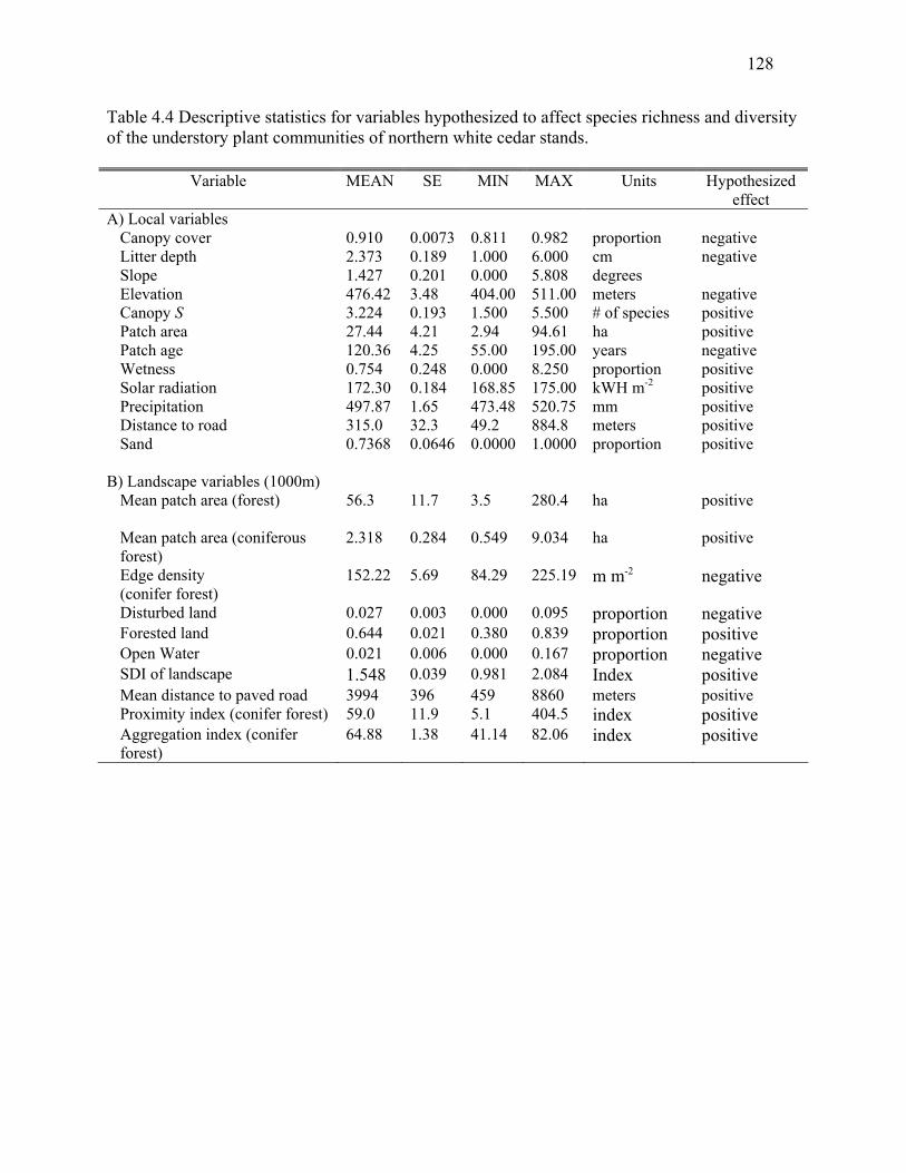
128

Table 4.4 Descriptive statistics for variables hypothesized to affect species richness and diversity of the understory plant communities of northern white cedar stands.

Variable MEAN SE MIN MAX Units Hypothesized effect

A) Local variables Canopy cover 0.910 0.0073 0.811 0.982 proportion negative Litter depth 2.373 0.189 1.000 6.000 cm negative Slope 1.427 0.201 0.000 5.808 degrees Elevation 476.42 3.48 404.00 511.00 meters negative Canopy S 3.224 0.193 1.500 5.500 # of species positive Patch area 27.44 4.21 2.94 94.61 ha positive Patch age 120.36 4.25 55.00 195.00 years negative Wetness 0.754 0.248 0.000 8.250 proportion positive Solar radiation 172.30 0.184 168.85 175.00 kWH m-2 positive Precipitation 497.87 1.65 473.48 520.75 mm positive Distance to road 315.0 32.3 49.2 884.8 meters positive Sand 0.7368 0.0646 0.0000 1.0000 proportion positive

B) Landscape variables (1000m) Mean patch area (forest) 56.3

11.7 3.5 280.4 ha positive

Mean patch area (coniferous forest)

2.318 0.284 0.549 9.034 ha positive

Edge density (conifer forest)

152.22 5.69 84.29 225.19 m m-2 negative

Disturbed land 0.027 0.003 0.000 0.095 proportion negative Forested land 0.644 0.021 0.380 0.839 proportion positive Open Water 0.021 0.006 0.000 0.167 proportion negative SDI of landscape 1.548 0.039 0.981 2.084 Index positive Mean distance to paved road 3994 396 459 8860 meters positive Proximity index (conifer forest) 59.0 11.9 5.1 404.5 index positive Aggregation index (conifer forest)

64.88 1.38 41.14 82.06 index positive

129

Table 4.5 Univariate ordinary least squares regression models of species richness for four vegetation growth forms (forbs, shrubs, seedlings and ferns). Variables significant at p <0.05 are shown in bold. Models use data with n = 38 except for litter depth which has only n=35. Response

Predictor variable

β ± SE

P

R2

R2

adj S forbs Litter depth -0.851 ± 0.360 0.024 14.5% 11.9% Wetness 0.688 ± 0.239 0.007 18.7% 16.4% Distance to road 0.004 ± 0.002 0.083 8.1% 5.6% Proportion disturbed -42.3 ± 17.8 0.023 13.6% 11.2% Proportion open water -20.8 ± 9.82 0.041 11.1% 8.6% S shrubs Proportion disturbed -18.8 ± 7.78 0.021 13.9% 11.5% Canopy cover -0.0664 ± 0.0380 0.089 7.8% 5.2% Canopy S -0.377 ± 0.135 0.008 17.8% 15.5% S seedlings Mean patch area (forest) 0.00693 ± 0.00368 0.068 9.0% 6.4% Canopy S 0.443 ± 0.221 0.052 10.1% 7.6%

Sand 1.52 ± 0.650 0.024 13.3% 10.9% S ferns

Proximity Index (conifer forest) 0.00362 ± 0.00201 0.081 8.2% 5.7% Solar radiation -0.257 ± 0.129 0.054 9.9% 7.4% Precipitation 0.0342 ± 0.0140 0.020 14.2% 11.8% Litter depth -0.392 ± 0.124 0.003 23.2% 20.9%

130

Table 4.6 Results of top regression models (representing 95% of Akaike weights) for species richness of forbs (S forbs), shrubs (S shrubs), seedlings (S seedlings) and ferns (S ferns). Model description

R2

adj

AICc

∆AICc

wi S forbs

Litter depth, wetness, proportion disturbed 39.1% 154.007 0.0000 0.36482Litter depth, wetness, proportion disturbed, proportion open water

40.6% 155.078 1.0710 0.21356

Litter depth, wetness, distance to road, proportion disturbed

39.6% 155.686 1.6790 0.15758

Litter depth, wetness, distance to road, proportion disturbed, proportion open water

40.5% 157.313 3.3052 0.06988

Litter depth, proportion disturbed 29.3% 157.501 3.4940 0.06359Litter depth, proportion disturbed, proportion open water

32.0% 157.908 3.9005 0.05189

Litter depth, distance to road, proportion disturbed 30.1% 158.843 4.8358 0.03251S shrubs

Proportion disturbed, canopy S 19.6% 110.672 0.0000 0.29956Canopy S 15.5% 111.068 0.3960 0.24575Proportion disturbed, canopy cover 17.0% 111.873 1.2019 0.16425Proportion disturbed 11.5% 112.800 2.1282 0.10336Proportion disturbed, canopy cover, canopy S 18.1% 113.056 2.3847 0.09092Canopy cover, canopy S 13.1% 113.631 2.9591 0.06822

S seedlings Canopy S, sand 21.3% 143.807 0.0000 0.46271Mean patch area (forest), canopy S, sand 21.8% 145.241 1.4336 0.22595Sand 10.9% 147.013 3.2062 0.09313Mean patch area (forest), canopy S 13.8% 147.272 3.4644 0.08185Mean patch area (forest), sand 11.9% 148.106 4.2993 0.05392Canopy S 7.6% 148.427 4.6202 0.04592

S ferns Proximity index, precipitation, litter depth 31.7% 87.216 0.0000 0.24921Proximity index, litter depth 27.6% 87.522 0.3062 0.21383Proximity index, solar radiation, litter depth 29.9% 88.091 0.8752 0.16089Proximity index, solar radiation, precipitation, litter depth

32.2% 88.851 1.6351 0.11003

Litter depth 20.9% 89.037 1.8207 0.10028Precipitation, litter depth 23.3% 89.589 2.3730 0.07608Solar radiation, litter depth 22.0% 90.105 2.8887 0.05879

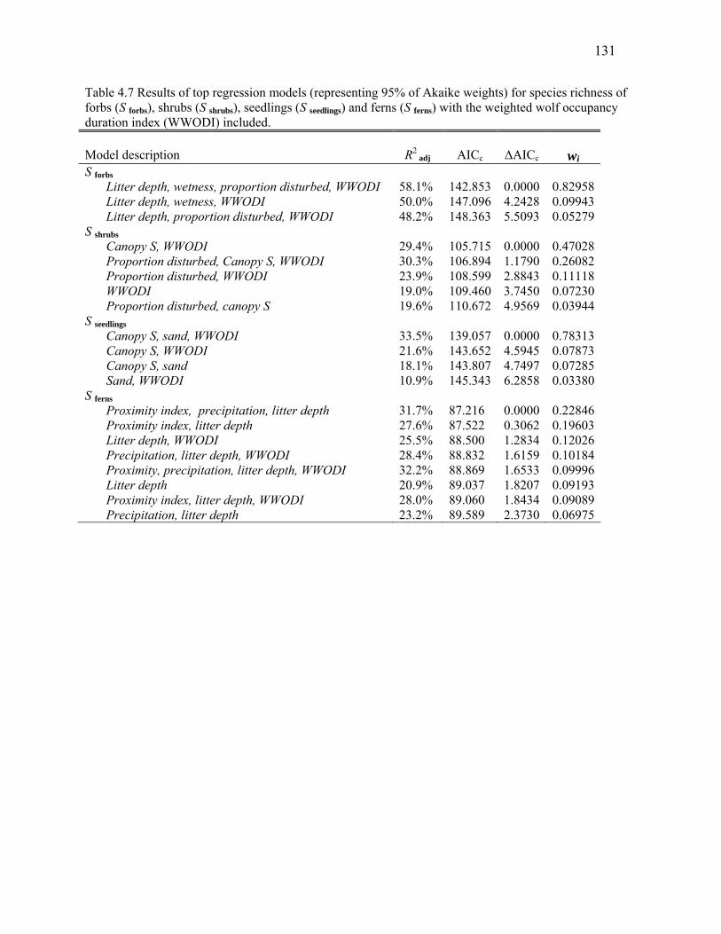
131

Table 4.7 Results of top regression models (representing 95% of Akaike weights) for species richness of forbs (S forbs), shrubs (S shrubs), seedlings (S seedlings) and ferns (S ferns) with the weighted wolf occupancy duration index (WWODI) included. Model description

R2

adj

AICc

∆AICc

wi S forbs

Litter depth, wetness, proportion disturbed, WWODI 58.1% 142.853 0.0000 0.82958Litter depth, wetness, WWODI 50.0% 147.096 4.2428 0.09943Litter depth, proportion disturbed, WWODI 48.2% 148.363 5.5093 0.05279

S shrubs Canopy S, WWODI 29.4% 105.715 0.0000 0.47028Proportion disturbed, Canopy S, WWODI 30.3% 106.894 1.1790 0.26082Proportion disturbed, WWODI 23.9% 108.599 2.8843 0.11118WWODI 19.0% 109.460 3.7450 0.07230Proportion disturbed, canopy S 19.6% 110.672 4.9569 0.03944

S seedlings Canopy S, sand, WWODI 33.5% 139.057 0.0000 0.78313Canopy S, WWODI 21.6% 143.652 4.5945 0.07873Canopy S, sand 18.1% 143.807 4.7497 0.07285Sand, WWODI 10.9% 145.343 6.2858 0.03380

S ferns Proximity index, precipitation, litter depth 31.7% 87.216 0.0000 0.22846Proximity index, litter depth 27.6% 87.522 0.3062 0.19603Litter depth, WWODI 25.5% 88.500 1.2834 0.12026Precipitation, litter depth, WWODI 28.4% 88.832 1.6159 0.10184Proximity, precipitation, litter depth, WWODI 32.2% 88.869 1.6533 0.09996Litter depth 20.9% 89.037 1.8207 0.09193Proximity index, litter depth, WWODI 28.0% 89.060 1.8434 0.09089Precipitation, litter depth 23.2% 89.589 2.3730 0.06975

132

Table 4.8 Coefficients table for the model averaged model for four vegetation growth forms (forbs, shrubs, seedlings and ferns) when the weighted wolf occupancy duration index is included in the global model. Response

Predictor variable

β ± SE

Upper 95%

Lower 95%

Parameter Importance

S forbs Litter depth -0.7564 ± 0.2694 -0.2284 -1.2844 0.99938 Wetness 0.5267 ± 0.1848 0.8888 0.1645 0.93283 Proportion disturbed -41.6173 ± 15.9057 -10.4421 -72.7926 0.88649 WWODI 0.3599 ± 0.0942 0.5445 0.1753 0.99622 S shrubs Proportion disturbed -10.9245 ± 7.93597 4.63005 -26.4790 0.42506 Canopy S -0.3022 ± 0.13075 -0.04595 -0.5585 0.80291 WWODI 0.1324 ± 0.04893 0.22833 0.0365 0.91459 S seedlings Canopy S 0.56616 ± 0.19507 0.94848 0.18383 0.94195 Sand 1.53012 ± 0.57438 2.65590 0.40434 0.90445

WWODI 0.19651 ± 0.07346 0.34049 0.05254 0.90525 S ferns

Proximity index 0.00345 ± 0.00182 0.0070 -0.0001 0.61589 Precipitation 0.02300 ± 0.01419 0.0508 -0.0048 0.50080 Litter depth -0.33033 ± 0.13765 -0.0605 -0.6001 0.99912 WWODI 0.06215 ± 0.04448 0.1493 -0.0250 0.41328

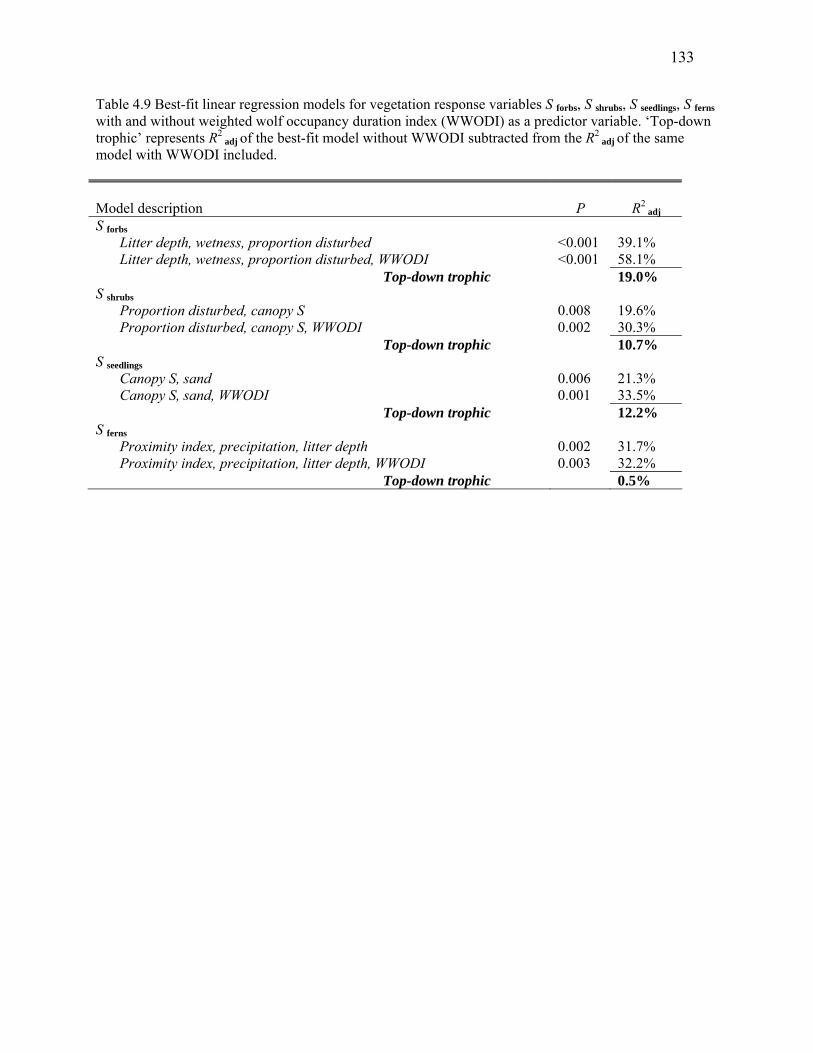
133

Table 4.9 Best-fit linear regression models for vegetation response variables S forbs, S shrubs, S seedlings, S ferns with and without weighted wolf occupancy duration index (WWODI) as a predictor variable. ‘Top-down trophic’ represents R2

adj of the best-fit model without WWODI subtracted from the R2 adj of the same

model with WWODI included. Model description

P

R2

adj

S forbs Litter depth, wetness, proportion disturbed <0.001 39.1% Litter depth, wetness, proportion disturbed, WWODI <0.001 58.1%

Top-down trophic 19.0% S shrubs

Proportion disturbed, canopy S 0.008 19.6% Proportion disturbed, canopy S, WWODI 0.002 30.3%

Top-down trophic 10.7% S seedlings

Canopy S, sand 0.006 21.3% Canopy S, sand, WWODI 0.001 33.5%

Top-down trophic 12.2% S ferns

Proximity index, precipitation, litter depth 0.002 31.7% Proximity index, precipitation, litter depth, WWODI 0.003 32.2%

Top-down trophic 0.5%

134

Table 4.10 Top regression model for weighted wolf occupancy duration index (WWODI) applied to vegetation response variables S forbs, S shrubs, S seedlings, S ferns. Model description

P

R2

adj Mean distance to paved road, mean patch area (coniferous forest)

S forbs 0.19 3.8%S shrubs 0.24 2.7%S seedlings 0.32 0.9%S ferns 0.21 3.3%

135

0 2 4 6 8 100

5

10

15

WWODI

Forb

Spe

cies

Ric

hnes

s

0 2 4 6 8 100

2

4

6

8

10

WWODI

Seed

ling

Spec

ies

Ric

hnes

s

0 2 4 6 8 100

1

2

3

4

5

WWODI

Fern

Spe

cies

Ric

hnes

s

0 2 4 6 8 100

2

4

6

WWODI

Shru

b Sp

ecie

s R

ichn

ess

Figure 4.1 Univariate relationships between S of forbs, shrubs, seedlings, ferns and the weighted wolf occupancy duration index (WWODI). Ordinary least squares regression lines and confidence bands (95%) are shown for all variables.

136

1 2 3 4 5 60

5

10

15

20

Litter Depth (cm)

Forb

Spe

cies

Ric

hnes

s

0 2 4 6 8 100

5

10

15

20

% Standing Water in Plot

Forb

Spe

cies

Ric

hnes

s

0.00 0.02 0.04 0.06 0.08 0.100

5

10

15

20

Proportion Disturbed Cells in Landscape

Forb

Spe

cies

Ric

hnes

s

0 200 400 600 800 10000

5

10

15

20

Distance from Road (m)

Forb

Spe

cies

Ric

hnes

s

0.00 0.05 0.10 0.15 0.200

5

10

15

20

Proportion Water Cells in Landscape

Forb

Spe

cies

Ric

hnes

s

Figure 4.2 Univariate relationships between S of forbs at the 10m2 scale and independent variables with P < 0.10. Ordinary least squares regression lines and confidence bands (95%) are shown for all variables.

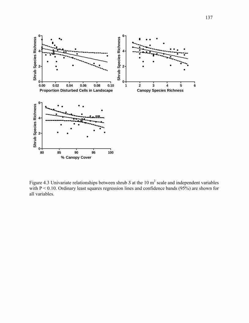
137

0.00 0.02 0.04 0.06 0.08 0.100

2

4

6

Proportion Disturbed Cells in Landscape

Shru

b Sp

ecie

s R

ichn

ess

1 2 3 4 5 60

2

4

6

Canopy Species Richness

Shru

b Sp

ecie

s R

ichn

ess

80 85 90 95 1000

2

4

6

% Canopy Cover

Shru

b Sp

ecie

s R

ichn

ess

Figure 4.3 Univariate relationships between shrub S at the 10 m2 scale and independent variables with P < 0.10. Ordinary least squares regression lines and confidence bands (95%) are shown for all variables.

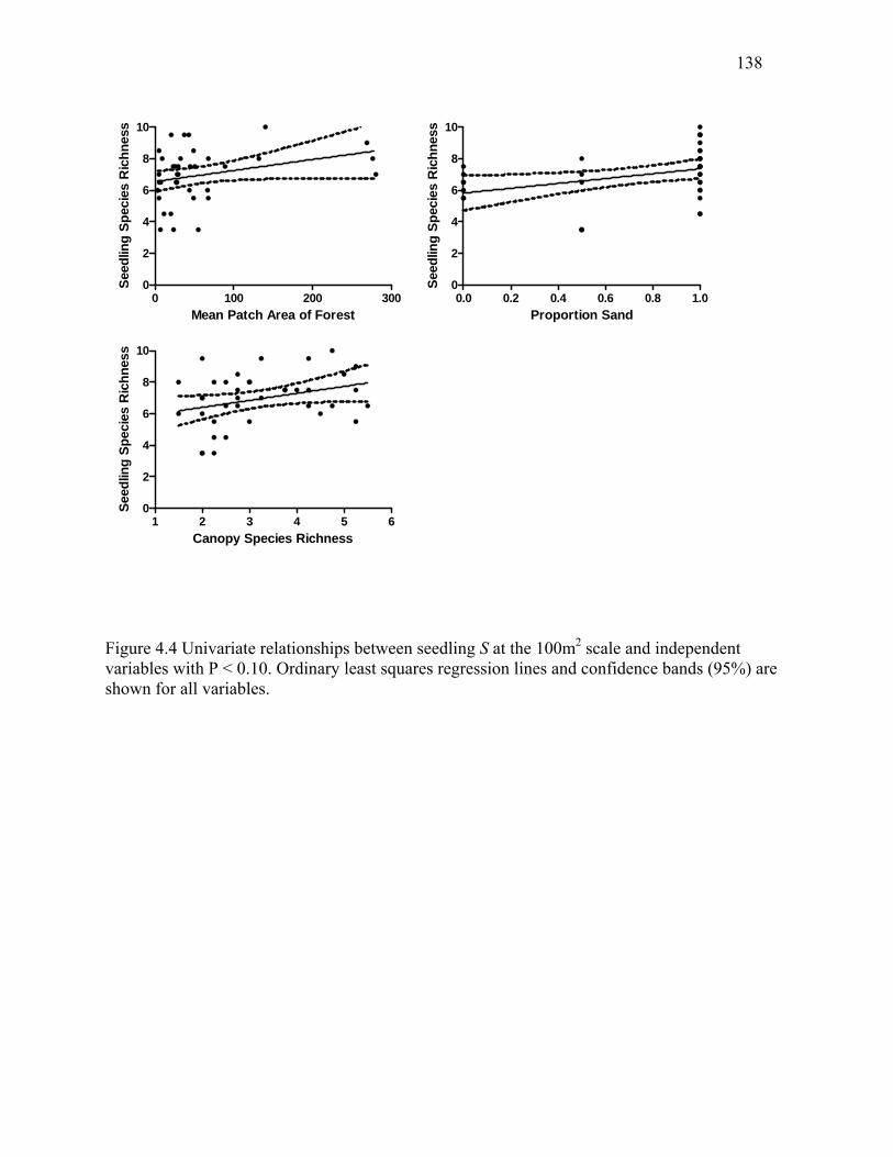
138

1 2 3 4 5 60

2

4

6

8

10

Canopy Species Richness

Seed

ling

Spec

ies

Ric

hnes

s

0 100 200 3000

2

4

6

8

10

Mean Patch Area of Forest

Seed

ling

Spec

ies

Ric

hnes

s

0.0 0.2 0.4 0.6 0.8 1.00

2

4

6

8

10

Proportion Sand

Seed

ling

Spec

ies

Ric

hnes

s

Figure 4.4 Univariate relationships between seedling S at the 100m2 scale and independent variables with P < 0.10. Ordinary least squares regression lines and confidence bands (95%) are shown for all variables.

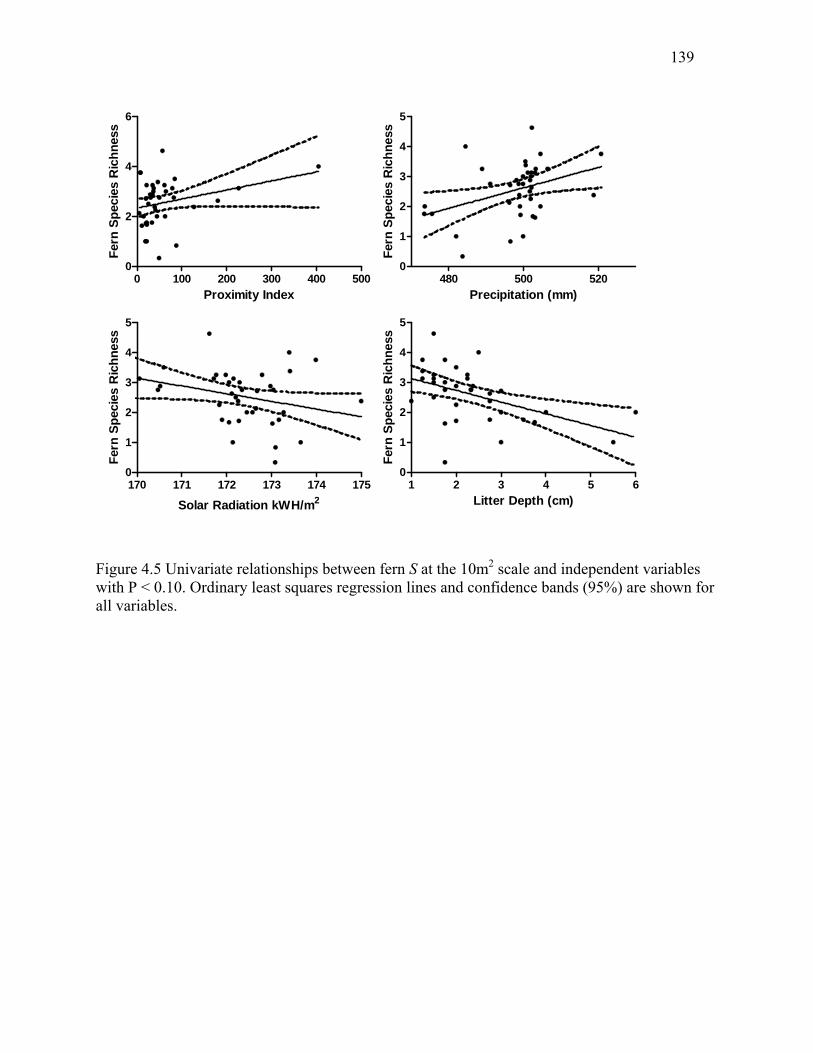
139

0 100 200 300 400 5000

2

4

6

Proximity Index

Fern

Spe

cies

Ric

hnes

s

480 500 5200

1

2

3

4

5

Precipitation (mm)

Fern

Spe

cies

Ric

hnes

s

1 2 3 4 5 60

1

2

3

4

5

Litter Depth (cm)

Fern

Spe

cies

Ric

hnes

s

170 171 172 173 174 1750

1

2

3

4

5

Solar Radiation kWH/m2

Fern

Spe

cies

Ric

hnes

s

Figure 4.5 Univariate relationships between fern S at the 10m2 scale and independent variables with P < 0.10. Ordinary least squares regression lines and confidence bands (95%) are shown for all variables.

140

0 2 4 6 8 100

5

10

15

Mean Patch Area of Coniferous Forest

WW

OD

I

0 20 40 60 80 1000

5

10

15

Cedar Stand Area (ha)

WW

OD

I

0 2000 4000 6000 8000 100000

5

10

15

Mean Distance to Paved Road (m)

WW

OD

I

Figure 4.6 Univariate relationships between WWODI and independent variables with P < 0.10. Ordinary least squares regression lines and confidence bands (95%) are shown for all variables.

141

CHAPTER 5

CONCLUSION

Wolf recovery in the Great Lakes region presents an opportunity to observe how top

predators influence biodiversity of lower trophic levels and ecosystem properties. There has been

limited experimental evidence of trophic cascades initiated by vertebrate predators in temperate

terrestrial ecosystems, partly due to the difficulty in administering and monitoring such large

scale manipulations (Shurin et al. 2002). Recent attempts to infer top-down effects of predators

have drawn on comparisons across areas with and without predators (Berger et al. 2001), or

correlative studies of vegetation response following predator restoration (Ripple et al. 2001,

Ripple and Beschta 2003).

Most of these previous studies of top-down trophic effects of wolves used wolf presence

and/or predation risk by wolves as a dichotomous variable in either space or time (Ripple et al.

2001, Ripple and Beschta 2003, Ripple and Beschta 2004, Hebblewhite et al. 2005, Ripple and

Beschta 2006, Beschta and Ripple 2007, Beyer et al. 2007). Here we provide wolf impact as a

gradient representing the historic spatial extents of wolf pack territories through time since

colonization. Plant species are thought to recover slowly from disturbance (Foster 1992, Pearson

et al. 1998), so current vegetation conditions will reflect historic disturbance patterns, making a

gradient in space and time a more appropriate variable for measuring top-down trophic effects.

By addressing wolf impact at the scale of wolf territory extents, instead of presence/absence of

142

wolves for entire regions, we were able to have both replication of “treatments” and comparable

local control sites.

Ecological processes (such as trophic cascades) are likely to manifest differentially over a

range of spatial and temporal scales (Levin 1992, Polis 1999, Bowyer and Kie 2006). Levin

(2000) argues that we must develop experimental research designs that measure patterns of

variability in space and time if we are to understand how ecological processes interact to

structure ecosystems and drive community dynamics. By sampling at multiple spatial scales, we

revealed that changes in species richness are not consistent across scales nor among vegetation

growth forms: forbs show a stronger response at local scales (1-10m2), while shrubs show a

response across broader scales (10m2 - 400m2). The design of future research should incorporate

the proper scale in order to effectively detect top-down effects

For northern white-cedar wetlands, we found density and species diversity of woody

stems 50-100cm tall to be ideal plant response variables with which to measure release from

browsing pressure, especially when allowances were made for variability in species specific

browsing response. The gap in the size structure of woody stems characteristic of over-browsed

understories was less apparent in cedar wetlands with high potential wolf impact. However,

regardless of wolf impact, recruitment of cedar in lowland cedar stands in our study area

continues to be very limited. Alverson et al. (1988) concluded that deer densities need to be

maintained below 1-2/km2 in order to sustain the diversity of native Wisconsin plants. In our

study area, maximum deer densities of 13/km2 and above are common. It is unlikely that the

recovery of the wolf population alone will reduce the deer population to densities recommended

by Alverson et al. (1988). However, as the proportion of early successional forests decreases

143

across the Great Lakes Region, reduced forage, when combined with predation by wolves and

bears, may cause deer densities to naturally decline.

Top-down and bottom-up forces are both critical for maintaining biodiversity and

ecological integrity of ecosystems, but it is not well understood how the relative strengths of

these processes vary in space and time. Carnivores may cause herbivores to switch habitats or

change their foraging behavior, resulting in net-positive indirect effects on some plant

populations and net-negative indirect effects on other plant populations (Polis 1999). In addition,

the potential for confounding variables to produce spurious associations can cause serious

complications when interpreting the results of space-for-time studies such as this one. To address

these issues, we incorporated local and landscape level factors thought to impact our vegetation

response variables and employed model selection using an information theoretic approach.

Through this process, we showed a lack of evidence for competing explanations (bottom-up and

non-trophic) for the positive relationship we found between wolf occupancy duration and plant

species richness of forbs, shrubs and seedlings.

Total trophic-level biomass, a sufficient response variable for aquatic systems, may be an


Recent evidence suggests that the indirect effects of predators in terrestrial systems are much

stronger on plant species diversity than on plant biomass, and that these changes in species

composition and evenness have strong effects on ecosystem properties (Schmitz 2006). Thus, we

need to rethink how we address trophic cascades in terrestrial systems as opposed to

characterizing them as weaker examples of aquatic cascades (sensu Strong 1992, Halaj and Wise

2001, Shurin et al. 2002). If we fail to do so, we risk measuring the wrong plant response

variables and missing evidence of ecologically important trophic cascades in terrestrial systems.

144

Our data from northern white cedar wetlands support Schmitz’s argument that species diversity,

richness and composition are more meaningful measures of trophic level responses in terrestrial

systems.

Whether the differences we observed in vegetation patterns are due to direct predation on

ungulates (density mediated indirect effects) or to the indirect effect of wolves on deer foraging

behavior (trait mediated indirect effects) continues to be hotly debated (Ripple and Beschta 2004,

Beyer et al. 2007, Creel and Christianson 2009, Kaufmann et al. 2010) and is beyond the scope

of this study. We suspect, however, that density mediated indirect effects may be unlikely given

that the current Wisconsin wolf population, which has grown to ~690 individuals (Wydeven and

Wiedenhoeft 2010), has the capacity to take only ~12,000 deer per year. There are an estimated

390,000 deer in the Northern Forests of Wisconsin (posthunt), so region-wide effects of wolf

recovery on deer populations are unlikely to manifest in the short term. Trait mediated indirect

effects may be the more likely mechanism responsible for higher density and diversity of woody

stems in high impact wolf areas.

Unfortunately, reciprocal relationships between wolves, deer and vegetation are still

lacking. At present, deer data is available for the past several decades, but only at the very coarse

scale of deer management blocks (WiDNR 2009). Since most low and high wolf impact areas in

our study were within the same deer management unit, existing deer data was not ideal for the

scale of this study. Future research should focus on monitoring deer abundance and/or foraging

behavior concurrent with wolf occupancy and vegetation response.

Future research should also explicitly examine whether the response of deer to wolf

recovery is behavioral or numerical. If deer response to wolf recovery is purely behavioral, it is

possible that the presence of wolves simply alters the pattern of browsing intensity experienced

145

by plant communities across the landscape. By increasing browsing pressure in the buffer zones

between packs and reducing browsing pressure within pack territory extents, wolves may have

an overall neutral impact on regional biodiversity. Alternatively, by providing refugia from deer,

wolves may prevent local extinctions of rare and browse sensitive plant species.

The loss of wolves as a keystone predator has contributed to a less desirable state for

understory plant communities in northern white-cedar wetlands. Our data suggests that the

recovery of wolves in northern Wisconsin can partially reverse this trend, at least in specific

community types where wolf packs have been continuously present for at least 8 years. Our

results provide compelling correlative evidence of top-down trophic effects generated by the

recovery of Wisconsin’s wolf population.

The methods employed here can be used to predict long-term, region-wide effects of

reintroducing top predators to other terrestrial systems. In addition, the spatially hierarchical

sampling design developed to analyze wildlife census data in conjunction with vegetation data

provides a template for addressing other broad scale ecological impacts. Regardless of the

process in question, multi-scale approaches allow us to determine the scale at which a pattern

becomes detectable. The ability to detect such signals above the ambient noise of ecological

variation is essential to understanding the relationship between pattern and process.

146

REFERENCES Alverson, W. S., Waller, D. M. and S. L. Solheim. 1988. Forests too deer - edge effects in northern Wisconsin. Conservation Biology 2:348-358. Berger, J., P. B. Stacey, L. Bellis, and M. P. Johnson. 2001. A mammalian predator-prey disequilibrium: how the extinction of grizzly bears and wolves affects the diversity of avian neotropical migrants. Ecological Applications 11:947-960. Beschta, R. L. and W. J. Ripple. 2007. Wolves, elk, and aspen in the winter range of Jasper National Park, Canada. Canadian Journal of Forest Research 37:1873-1885. Beyer, H. L., E. H. Merrill, N. Varley, and M. S. Boyce. 2007. Willow on Yellowstone’s northern range: evidence for a trophic cascade? Ecological Applications 17:1563-1571. Bowyer, R.T., and J.G. Kie. 2006. Effects of scale on interpreting life-history characteristics of ungulates and carnivores. Diversity and Distributions 12:244-257. Creel, S., and D. Christianson. 2009. Wolf presence and increased willow consumption by Yellowstone elk: implications for trophic cascades. Ecology 90:2454-2466. Foster, D. R. 1992. Land-Use History (1730-1990) and Vegetation Dynamics in Central New England, USA. Journal of Ecology 80: 753-771. Halaj, J. and D. H. Wise. 2001. Terrestrial trophic cascades: How much do they trickle? The American Naturalist 157:262-281. Hebblewhite, M., White, C. A., Nietvelt, C. G., McKenzie, J. A., Hurd, T. E., Fryxell, J. M. et al. 2005. Human activity mediates a trophic cascade caused by wolves. Ecology 86:2135-2144. Kauffman, M. J., J. F. Brodie, and E. S. Jules. 2010. Are wolves saving Yellowstone's aspen? A landscape-level test of a behaviorally mediated trophic cascade. Ecology 91:2742-2755. Levin, S. A. 1992. The problem of pattern and scale in ecology. Ecology 73:1943-1967. Pearson, S. M., A. B. Smith, and M. G. Turner. 1998. Forest patch size, land use, and mesic forest herbs in the French Broad River Basin, North Carolina. Castanea 63:382–395. Polis, G. A. 1999. Why are parts of the world green? Multiple factors control productivity and the distribution of biomass. Oikos 86:3-15. Ripple, W. J., E. J. Larsen, R. A. Renkin and D. W. Smith. 2001. Trophic cascades among wolves, elk and aspen on Yellowstone National Park's northern range. Biological Conservation 102:227-234.

147

Ripple, W. J. and R. L. Beschta. 2003. Wolf reintroduction, predation risk, and cottonwood recovery in Yellowstone National Park. Forest Ecology and Management 184:299-313. Ripple, W. J. and R. L. Beschta. 2004. Wolves, elk, willows, and trophic cascades in the upper Gallatin Range of Southwestern Montana, USA. Forest Ecology and Management 200:161-181. Ripple, W. J. and R. L. Beschta. 2005. Linking Wolves and Plants: Aldo Leopold on Trophic Cascades. BioScience 55: 613-621. Ripple, W. J. and R. L. Beschta. 2006. Linking wolves to willows via risk-sensitive foraging by ungulates in the northern Yellowstone ecosystem. Forest Ecology and Management 230:96-106. Schmitz, O.J . 2006. Predators have large effects on ecosystem properties by changing plant diversity, not plant biomass. Ecology 87:1432-1437. Shurin, J. B., Borer, E. T., Seabloom, E. W., Anderson, K., Blanchette, C.A., Broitman, B. et al. 2002. A cross-ecosystem comparison of the strength of trophic cascades. Ecology Letters 5:785-791. Strong, D. R. 1992. Are trophic cascades all wet? Differentiation and donor control in a speciose system. Ecology 73:747-754. Wisconsin Department of Natural Resources 2009. Wisconsin DMU review: DMU reference materials. http://dmureview.editme.com/dmuref: Wisconsin Department of Natural Resources, Madison, WI, USA. Wydeven, A. P., and J. E. Wiedenhoeft. 2010. Gray wolf population, 2009-2010. Wisconsin Wildlife Surveys 16:140-155.

148

Appendix Species Name Growth form Athyrium filix-femina var. angustum Fern Botrychium virginianum Fern Dryopteris carthusiana Fern Dryopteris cristata Fern Dryopteris intermedia Fern Gymnocarpium dryopteris Fern Onoclea sensibilis Fern Osmunda cinnamomea Fern Osmunda claytoniana Fern Osmunda regalis var. spectabilis Fern Phegopteris connectilis Fern Pteridium aquilinum var. latiusculum Fern Fern Count 12Equisetum arvense Fern Ally Equisetum sylvaticum Fern Ally Huperzia lucidula Fern Ally Lycopodium annotinum Fern Ally Lycopodium dendroideum Fern Ally Fern Ally Count 5Actaea rubra Forb Anemone quinquefolia Forb Apocynum androsaemifolium Forb Aralia nudicaulis Forb Aralia racemosa Forb Arisaema triphyllum ssp. triphyllum Forb Aster ciliolatus Forb Aster macrophyllus Forb Caltha palustris Forb Campanula aparinoides Forb Chelone glabra Forb Chrysosplenium americanum Forb Cicuta maculata Forb Circaea alpina subsp. alpina Forb Cirsium muticum Forb Clintonia borealis Forb Comarum palustre Forb Coptis trifolia var. groenlandica Forb Corallorhiza striata Forb Corallorhiza trifida Forb Cornus canadensis Forb Cypripedium acaule Forb Cypripedium candidum Forb Cypripedium parviflorum Forb Doellingeria umbellata Forb Echinocystis lobata Forb Epilobium ciliatum Forb Epilobium coloratum Forb Eupatorium maculatum Forb Fragaria virginiana Forb

149

Species Name Growth form Galium tinctorium Forb Galium trifidum Forb Galium triflorum Forb Gaultheria hispidula Forb Gaultheria procumbens Forb Geum rivale Forb Goodyera repens Forb Impatiens capensis Forb Iris versicolor Forb Laportea canadensis Forb Linnaea borealis Forb Listera cordata Forb Lycopus americanus Forb Lycopus uniflorus Forb Lysimachia thyrsiflora Forb Maianthemum canadense Forb Maianthemum trifolium Forb Malaxis monophyllos var. brachypoda Forb Menyanthes trifoliata Forb Mitchella repens Forb Mitella diphylla Forb Mitella nuda Forb Moneses uniflora subsp. Uniflora Forb Monotropa hypopithys Forb Monotropa uniflora Forb Oxalis montana Forb Packera aurea Forb Platanthera clavellata Forb Platanthera obtusata Forb Polygala paucifolia Forb Polygonatum biflorum Forb Polygonatum pubescens Forb Polygonum arifolium Forb Polygonum cilinode Forb Prenanthes alba Forb Prunella vulgaris Forb Pyrola asarifolia subsp. asarifolia Forb Pyrola secunda Forb Ranunculus abortivus Forb Ranunculus acris Forb Ranunculus hispidus var. nitidus Forb Ranunculus recurvatus var. recurvatus Forb Rubus pubescens Forb Saxifraga pensylvanica Forb Scutellaria galericulata Forb Scutellaria lateriflora Forb Solidago uliginosa Forb Streptopus lanceolatus var. longipes Forb Symphyotrichum puniceum Forb Symplocarpus foetidus Forb Thalictrum dioicum Forb

150

Species Name Growth form Toxicodendron radicans var. negundo Forb Trentalis borealis Forb Trillium cernuum Forb Vaccinium oxycoccos Forb Viola blanda var. palustriformis Forb Viola macloskeyi subsp. pallens Forb Viola renifolia Forb Waldsteinia fragarioides Forb Forb Count 89Brachyelytrum erectum Grass Cinna latifolia Grass Poa palustris Grass Calamagrostis canadensis Grass Oryzopsis asperifolia Grass Bromus ciliatus L. Grass Elymus hystrix var. hystrix Grass Grass Count 7Cirsium palustre Non-native Hieracium aurantiacum Non-native Taraxacum officinale Non-native Veronica officinalis Non-native Non-native Count 4Luzula acuminata var. acuminata Rush Rush Count 1Carex arctata Sedge Carex brunnescens Sedge Carex communis Sedge Carex crinita Sedge Carex deflexa Sedge Carex disperma Sedge Carex interior Sedge Carex intumescens Sedge Carex leptalea Sedge Carex leptonervia Sedge Carex pedunculata Sedge Carex pennsylvanica Sedge Carex projecta Sedge Carex scoparia Sedge Carex stipata Sedge Carex trisperma Sedge Sedge Count 16Abies balsamea Tree Acer rubrum Tree Acer saccharum Tree Acer spicatum Tree Betula alleghaniensis Tree Betula papyrifera Tree Fraxinus nigra Tree Fraxinus pennsylvanica Tree Larix laricina Tree Picea glauca Tree

151

Species Name Growth form Picea mariana Tree Pinus strobus Tree Populus tremuloides Tree Prunus virginiana Tree Quercus bicolor Tree Quercus macrocarpa var. macrocarpa Tree Quercus rubra Tree Sorbus americana Tree Sorbus decora Tree Thuja occidentalis Tree Tilia americana var. americana Tree Tsuga canadensis Tree Ulmus americana Tree Tree Count 23Acer spicatum Shrub Alnus incana ssp. rugosa Shrub Amelanchier sp. 1 Shrub Cornus stolonifera Shrub Corylus americana Shrub Corylus cornuta Shrub Diervilla lonicera Shrub Ilex mucronata Shrub Ilex verticillata Shrub Kalmia polifolia Shrub Ledum groenlandicum Shrub Lonicera canadensis Shrub Lonicera oblongifolia Shrub Lonicera villosa Shrub Rhamnus alnifolia Shrub Ribes americanum Shrub Ribes americanum Shrub Ribes cynosbati Shrub Ribes glandulosum Shrub Ribes hirtellum Shrub Ribes hudsonianum Shrub Ribes hudsonianum Shrub Ribes lacustre Shrub Ribes triste Shrub Rubus idaeus Shrub Sambucus sp. 1 Shrub Vaccinium angustifolium Shrub Vaccinium myrtilloides Shrub Vaccinium myrtilloides Shrub Vaccinium oxycoccos Shrub Viburnum opulus Shrub Shrub Count 31Parthenocissus quinquefolia Vine Toxicodendron radicans subsp. negundo Vine Vine Count 2Grand Count 190

Documents

ARE WOLVES IN WISCONSIN AFFECTING THE BIODIVERSITY OF