Embed Size (px)
Citation preview

Are we going to survive?
Economic models of endogenous growth and evidence from global population and CO2 emission trends

2Andreas HueslerCCSS, 2009-10-24
Outline
Introduction
Economic Model I: IPAT Economic Model II: Cobb-Douglas
Conclusions
Discussion

3Andreas HueslerCCSS, 2009-10-24
Current Economic Footprint
Population (in mio)
Ecological Footprint
Biocapacity Ecological Reserve
High Income Countries 972 6.4 3.7 -2.7
Middle Income Countries 3098 2.2 2.2 -0.0
Low Income Countries 2371 1.0 0.9 -0.1
World 6476 2.7 2.1 -0.6
Soucre
: footp
rintn
etw
ork
.org
4Andreas HueslerCCSS, 2009-10-24
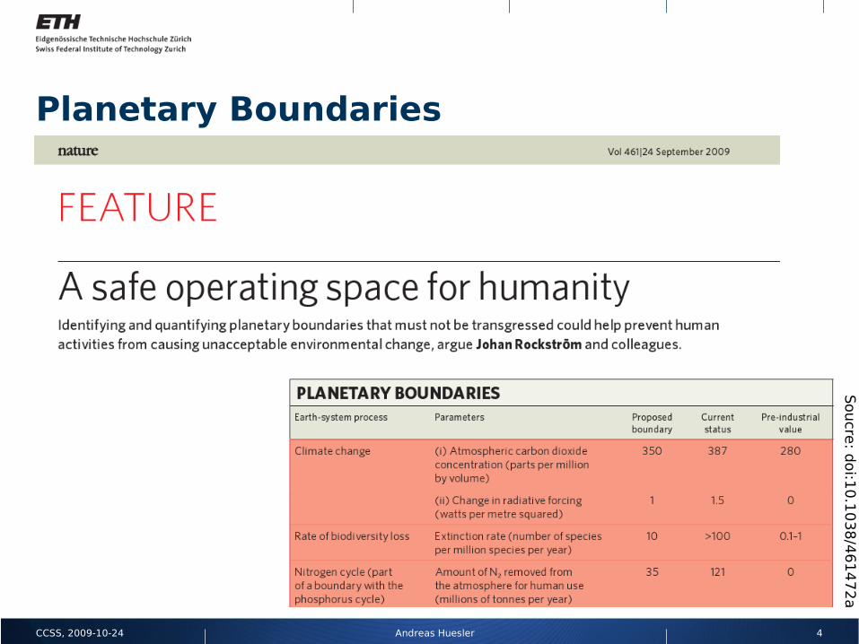
Planetary Boundaries
Soucre
: doi:1
0.1
038
/461
47
2a

5Andreas HueslerCCSS, 2009-10-24
ImPACT equation I: impact P: population A:affluence C:consumption T: technology
Economic Model I
CO2=Population×GDP
Population×EnergyGDP
×CO2Energy
Soucre
: doi: 1
0.1
07
3

6Andreas HueslerCCSS, 2009-10-24
Growth
Growth description:
Solving ODE:
dpdt
∝ p1
p t =p0tc−t −
0
0
=0
rel.
gro
wth
7Andreas HueslerCCSS, 2009-10-24
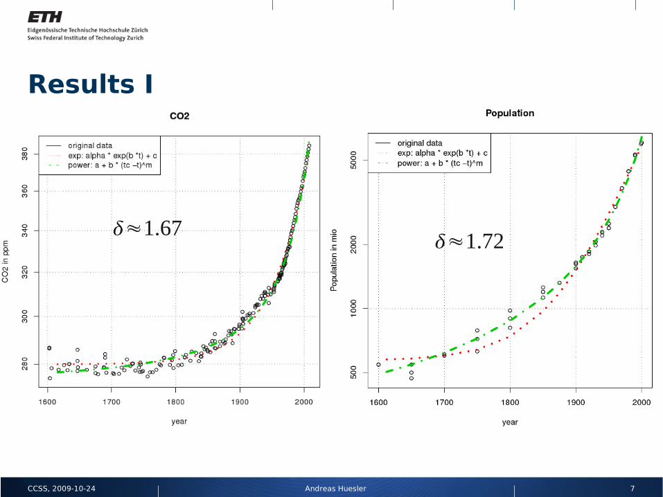
Results I
≈1.67≈1.72

8Andreas HueslerCCSS, 2009-10-24
Results II: Parameter stability
≈1.67
t c=t

9Andreas HueslerCCSS, 2009-10-24
Results II (cont)

10Andreas HueslerCCSS, 2009-10-24
Economic Models II
Cobb-Douglas: Y: output L: labour K: capital A: technology
Solow equation:
Y t =K t ×[ A t Lt ]1−
dAdt
=b K t ×L t ×A t
dKdt
=sY t =s K t ×A t L t 1−

11Andreas HueslerCCSS, 2009-10-24
Coupling ODE I
Assuming labour is proportional to capital (cf Kremer)
we getdAdt
=a' L t ×A t
dLdt
=b ' L t ×A t 1−
K t ≈L t

12Andreas HueslerCCSS, 2009-10-24
Coupling ODE II
Assuming solutions of the form:
Gives us by coefficient matching
A finite-time singularities can be created from the interplay of several growing variables resulting in a non-trivial behavior: the interplay between different quantities may produce an “explosion” in the population even though the individual dynamics do not!.
A t =A0 tc−t −
L t =L0tc−t −
=11−
=2−−
×
11−

13Andreas HueslerCCSS, 2009-10-24
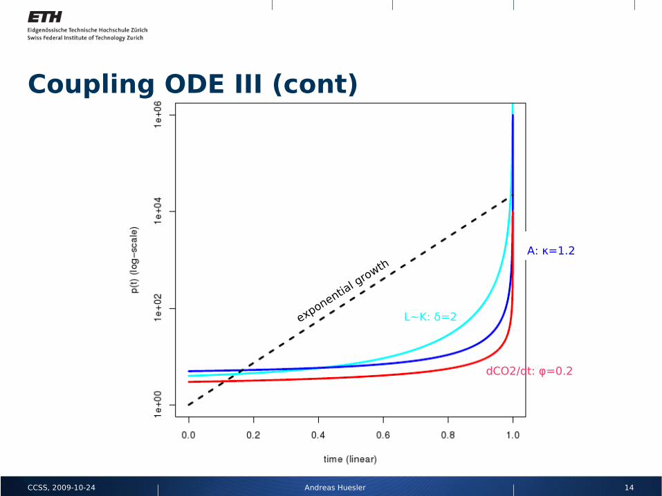
Coupling ODE III
For the cumulative CO2:
=> φ = -δα+κ
Numerical example:α=0.5, β=0.9, θ=0.9, γ=0.1=> δ=2, κ=1.2=> φ = 0.2 (>0, hence explosive)
dCO2dt
=Y t A t
=A0− L0
1×t c−t
−
14Andreas HueslerCCSS, 2009-10-24
Coupling ODE III (cont)
exponential g
rowth
L~K: δ=2
A: κ=1.2
dCO2/dt: φ=0.2
15Andreas HueslerCCSS, 2009-10-24
Conclusions
Dynamics of CO2 emissions can have complicated dynamics
The (non-linear) dynamics can lead to finite time singularities
Any scenario for future CO2 emissions should take econmic and population dynamics into account.

16Andreas HueslerCCSS, 2009-10-24
References
More references available at:http://www.citeulike.org/user/ahuesler

17Andreas HueslerCCSS, 2009-10-24
Reserve ....

18Andreas HueslerCCSS, 2009-10-24
Case Study: Easter Islands (II)
Colonization Rapid Growth Collapse
Carrying Capacity / Resources
Economic Activity / GDP
Population
400 AD 1600 AD 1750 AD
Soucre
: wikip
edia
, Dia
mond, o
wn g
raphic

19Andreas HueslerCCSS, 2009-10-24

20Andreas HueslerCCSS, 2009-10-24
Source: xkcd.com