FEDERAL RESERVE BANK OF SAN FRANCISCO

WORKING PAPER SERIES

The views in this paper are solely the responsibility of the author and should not be interpreted as reflecting the views of the Federal Reserve Bank of San Francisco or the Board of Governors of the Federal Reserve System. This paper was produced under the auspices of the Center for Pacific Basin Studies within the Economic Research Department of the Federal Reserve Bank of San Francisco.

http://www.frbsf.org/publications/economics/papers/2006/wp06-13bk.pdf

Are There Productivity Spillovers

from Foreign Direct Investment in China?

Galina Hale Federal Reserve Bank of San Francisco

Cheryl Long Colgate University

February 2007

Are there Productivity Spillovers from Foreign Direct Investment in China?

Galina Hale∗

Federal Reserve Bank of San Francisco

Cheryl Long†

Colgate University

February 2007

Abstract

We review previous literature on productivity spillovers of foreign direct investment (FDI) in Chinaand conduct our own analysis using a firm–level data set from a World Bank survey. We find that theevidence of FDI spillovers on the productivity of Chinese domestic firms is mixed, with many positiveresults largely due to aggregation bias or failure to control for endogeneity of FDI. Attempting over2500 specifications which take into account forward and backward linkages, we fail to find evidence ofsystematic positive productivity spillovers from FDI.

JEL classification: L33, F23, O17

Keywords: FDI, spillovers, forward–backward linkages, China

∗galina.b.hale@sf.frb.org. Hale is grateful to the Stanford Center for International Development for financial support andhospitality during work on this project.

†cxlong@mail.colgate.edu. Long thanks the Hoover Institution for financial support and hospitality during work on thisproject.

We thank Robert Deckle, Bob Hall, Oscar Jorda, Ted Moran, Bob Turner, Bin Xu, Kent Zhao and the participants ofthe ASSA session on“Understanding the Mechanisms of China’s Economic Growth” for invaluable suggestions and ChrisCandelaria for outstanding research assistance. We are grateful to Runtian Jing for sharing the data. All errors are ours. Theviews in this paper are solely the responsibility of the authors and should not be interpreted as reflecting the views of theFederal Reserve Bank of San Francisco.

1

1 Introduction

China has been extremely successful in attracting foreign direct investment (FDI) since it started the eco-

nomic reforms at the end of the 1970s. Figure 1 illustrates the breathtaking speed of FDI growth in China.

Annual FDI inflow was below $100 million in 1979, but exceeded $580 billion in 2006, with an annual growth

rate of close to 30%. Such rapid growth of FDI inflow has largely been accompanied by government policies

that encourage FDI, as described in detail in Hale and Long (2006). Some of these policies aimed to equalize

operating conditions for foreign capital inside and outside China, including those regarding foreign trade and

foreign exchange control. Other policies provided monetary incentives for foreign investors, including prefer-

ential treatment in taxation and environmental regulation. While policies that level the playing grounds for

foreign firms operating outside and inside China are prerequisites for capital inflow that seeks higher rate

of returns, the policies that subsidize foreign investors through lower tax rates and lenient environmental

requirements can only be justified if positive externalities on domestic firms are created with the inflow of

FDI (Moran, 2007).

Although FDI growth and the effectiveness of government policies in prompting such growth have been

unrefuted, the effects of FDI on domestic firms are far from clear. Previous studies on FDI spillover effects on

productivity of Chinese firms have produced mixed evidence as to whether domestic firms have benefited from

FDI presence. Due to limited availability of the firm–level panel data and difficulty in finding instruments

for FDI presence, many positive results obtained by researches suffer from an upward bias due to aggregation

or endogeneity of FDI.

In this paper we discuss these and other potential biases that arise in existing literature on FDI spillovers

in China. We also conduct our own analysis using a data set from a World Bank stratified survey of firms

in five cities and ten industries. While our data set lacks time dimension, it contains very rich information

on many aspects of firms’ state and behavior. In addition to limiting the sample to domestic firms, which

removes the aggregation bias, we apply instrumental variables analysis to address potential endogeneity of

FDI presence, using three variables that do not affect domestic firms’ productivity directly. We also control

for non–random selection that arises when limiting the sample to domestic firms and could bias estimates

downward. After controlling for these biases, we fail to find any significant FDI spillover effects on TFP or

labor productivity for domestic firms in the same, upstream or downstream industries.

We believe that there are institutional factors that may explain the lack of productivity spillovers of FDI

in China. For instance, one important channel of spillovers is technology transfer through labor mobility.

In China, however, labor mobility across regions and industries is still limited due to formal labor market

2

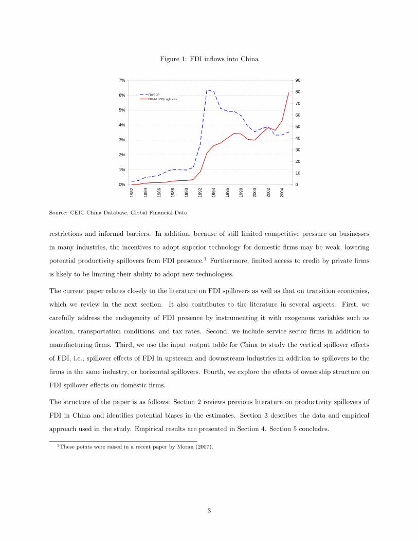
Figure 1: FDI inflows into China

0%

1%

2%

3%

4%

5%

6%

7%

1982

1984

1986

1988

1990

1992

1994

1996

1998

2000

2002

2004

0

10

20

30

40

50

60

70

80

90

FDI/GDPFDI (bil.USD): right axis

Source: CEIC China Database, Global Financial Data

restrictions and informal barriers. In addition, because of still limited competitive pressure on businesses

in many industries, the incentives to adopt superior technology for domestic firms may be weak, lowering

potential productivity spillovers from FDI presence.1 Furthermore, limited access to credit by private firms

is likely to be limiting their ability to adopt new technologies.

The current paper relates closely to the literature on FDI spillovers as well as that on transition economies,

which we review in the next section. It also contributes to the literature in several aspects. First, we

carefully address the endogeneity of FDI presence by instrumenting it with exogenous variables such as

location, transportation conditions, and tax rates. Second, we include service sector firms in addition to

manufacturing firms. Third, we use the input–output table for China to study the vertical spillover effects

of FDI, i.e., spillover effects of FDI in upstream and downstream industries in addition to spillovers to the

firms in the same industry, or horizontal spillovers. Fourth, we explore the effects of ownership structure on

FDI spillover effects on domestic firms.

The structure of the paper is as follows: Section 2 reviews previous literature on productivity spillovers of

FDI in China and identifies potential biases in the estimates. Section 3 describes the data and empirical

approach used in the study. Empirical results are presented in Section 4. Section 5 concludes.

1These points were raised in a recent paper by Moran (2007).

3

2 Review of empirical literature

Theoretical work has generally predicted positive effects of FDI presence on domestic firms’ productivity

through the labor mobility channel (Kaufmann, 1997; Haaker, 1999; Fosfuri, Motta, and Rønde, 2001; Glass

and Saggi, 2002) or through competition and demostration effects (Wang and Blomstrom, 1992). These

models predict same–industry, or horizontal, spillovers. In addition, Rodriguez-Clare (1996) outlines for-

ward and backward linkages between foreign firms and domestic firms as a possible mechanism for positive

spillovers.

However, the results from empirical studies are mixed. Most studies focus on the spillover effects of FDI

on domestic firms in the same industry. For example, among the 42 studies on horizontal productivity

spillovers of FDI in developed, developing, and transition economies summarized in Gorg and Greenaway

(2004), only 20 studies report unambiguously positive and significant results. Furthermore, 14 out of the 20

studies finding positive effects either use cross–section data at the industry level, which leads to aggregation

bias we discuss below, or use cross–section of firm level data without controlling for the endogeneity of FDI

presence. Among the 24 studies using firm level panel data, which Gorg and Greenaway (2004) argue to

be the most appropriate estimating framework, only 5 obtain positive and significant FDI spillover effects,

with 4 from developed countries. For transition economies, only one out of the 8 studies discussed obtains

positive and significant FDI spillover effects, using cross–section data.

The results appear more conclusive for vertical spillovers. Among the five studies discussed in Gorg and

Greenaway (2004) that focus on vertical FDI spillover effects, i.e., effects of FDI presence on domestic firms

located in upstream or downstream firms, three find positive backward FDI spillovers, one finds positive

forward FDI spillovers. In addition Javorcik (2004) and Blalock and Gertler (2007) find positive vertical

FDI spillovers in Latvia and Indonesia, respectively.

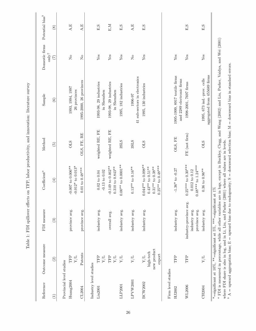
Similar to findings for other countries, studies on FDI spillover effects in China have obtained a wide range

of estimates for the effects of FDI presence on the productivity of Chinese domestic firms. We summarize

published studies of FDI spillover effects on productivity of Chinese firms in Table 1. As shown in Column

(2), most studies of FDI spillover effects in China focus on how the presence of FDI affects the total factor

productivity (TFP) of domestic firms, their labor productivity or both, with the exception of Cheung and

Lin (2004), which studies patent applications, and Buckley, Clegg, and Wang (2002), which include high-tech

and new product development as well as export performance in addition to labor productivity.

4

2.1 Potential biases in empirical literature

Before discussing the results of the empirical studies on FDI spillovers in China, we would like to address the

biases that may arise when estimating the effect of foreign presence on the productivity of domestic firms.

To fix ideas, suppose that there are I industries indexed i = {1, ...I},2 each containing Ni firms. Suppose

Mi < Ni of these firms are domestic and the rest are foreign–invested (which we will call foreign, for short).

The most common measure of FDI presence in industry i is then

FDIi =

∑Ni

j=Mi+1wj∑Ni

j=1 wj

,

where wj is some weight (usually employment or sales), indicating the size of each firm. Thus, FDIi is

size–weighed share of foreign firms in industry i.3

To simplify the discussion, and without loss of generality, assume that all firms have the same size, and

therefore

FDIi =Ni −Mi

Ni.

The most common way to estimate the FDI spillover effect is by fitting the regression

yji = α + βFDIi + γ lji + δkji + εji, (1)

where yji = log Yji is log of value added by firm j from industry i, lji = log Lji is log of employment,

kji = log Kji is log of capital. This approach assumes the production function of the form Yji = AjiLγjiK

δji,

where log Aji = α+βFDIi+εji = ai+εji is a log of total factor productivity of firm j from industry i, which

has an industry–specific component ai that is tested for being linked to the presence of FDI in the industry.

Thus, α is a common component, or mean TFP, β measures the extent of spillovers from FDI presence,

while εji is a mean–zero firm–specific error term assumed to be orthogonal to FDIi.4 The hypothesis being

tested is H0: β > 0.

Aggregation bias

2These can also be interpreted as cities, provinces, industry–province or industry–city cells.

3Alternatively, the numerator can bePNi

j=1 wjsj , where sj is the share of foreign ownership in firm j, or the share ofownership by the largest foreign partner, the measure we adopt in our own regressions, below.

4A common alternative is to estimate yji − lji = α+ δFDIi + δ(kji − lji)+ εji, which assumes, in addition, constant returnsto scale.

5

Suppose that the firm–level data is not available, as it is commonly the case, and therefore estimation is

conducted at the aggregated level, i-level, for instance, by province or industry. An important assumption in

the FDI spillover literature is that foreign–invested firms have better technology that spills over to domestic

firms through various channels. Thus, it is assumed that foreign–invested firms are more productive than

firms without foreign partners.5 In the studies that use aggregate data, foreign firms are frequently not

excluded from the aggregates, thus, using our notation, the following equation is estimated,

yi = α + βFDIi + γli + δki + εi, (2)

where yi = 1/Ni

∑Ni

j=1 yji, li = 1/Ni

∑Ni

j=1 lji, ki = 1/Ni

∑Ni

j=1 kji.

Suppose all the firms are identical in all respects, except that all foreign firms’ TFP is higher by a constant.

Denoting domestic firms with superscript d and foreign firms with superscript f , Y di = Ad

i Lγi Kδ

i , Y fi =

Afi Lγ

i Kδi , with Af

i > Adi ,∀i. This also implies that af

i = log Afi > ad

i = log Adi . Then, by construction, the

higher is the share of foreign firms, the higher is the aggregated measure of TFP:

ai =Mi

Niad

i +Ni −Mi

Niaf

i = (1− FDIi)adi + FDIia

fi = ad

i + FDIi(afi − ad

i ),

so that ∂ai/∂FDIi > 0 whenever afi > ad

i . Thus, when estimating Equation (2) at the aggregated level

across i with ai = α + βFDIi, one automatically finds β > 0, even if individual domestic firms’ TFP is not

affected by the presence of FDI. In other words, the estimates of spillover effects obtained from aggregate

regressions are subject to an upward aggregation bias that can be avoided by excluding foreign firms from

the aggregates or using firm–level data.

Selection bias

Unfortunately, estimating the model on the subset of domestic firms, or using the aggregates that exclude

foreign–ivestment firms is not without flaws either. The first problem arises due to the very likely possibility

of non–random selection.

Suppose relevant FDI are mergers and acquisitions (M&A) rather than greenfield investment. Further

suppose that foreign firms choose to invest in domestic firms that are more productive ex ante (the cherry–

picking phenomenon we already referred to), as opposed to investing at random and making firms more

5Because of the “cherry–picking” phenomenon, when foreign investor choose to invest in the first that are a priori moreproductive, it is notoriously difficult to show empirically the productivity effects of foreign ownership. In a notable exception,Arnold and Javorcik (2005) show, for the case of Indonesia, that foreign–invested firms perform better than similar domesticfirms.

6

productive ex post. We can rank all domestic firms in industry i before the FDI according to their TFP,

so that A1i < A2i < ...ANi, ∀i ∈ [1, I]. For simplicity, suppose that distribution of Aji is the same for all

industries and that the distribution of industry–level foreign investment across industries is orthogonal to

the distribution of Aji.

Cherry–picking implies that foreign capital flows to the firms in the upper tail of Aji distribution. Thus,

the TFP distribution of the firms that remain domestic after FDI inflow is upper–truncated. Moreover, the

truncation point Mi is lower the higher is the share of FDI firms in the industry. Thus, ai = 1/Mi

∑Mi

j=1 aji

is lower the lower is the share of domestic firms (i.e. the higher is the share of FDI), and ∂ai/∂FDIi < 0. As

a result, when Equation (1) is estimated for domestic firms only, with ai = α + βFDIi, one automatically

finds β < 0, in the absence of actual FDI spillovers. In other words, firm–level cross–section regressions that

are limited to domestic firms yield estimates of productivity spillovers of FDI that are biased downward if

cherry–picking is present. It is easy to see that the same is true for aggregate analysis that excludes foreign

firms from the aggregates.

The problem of selection bias can be addressed by estimating a model of sample selection, which allows

for the selection of the firms into domestic and foreign categories to be correlated with firms’ productivity.

Of course, this approach would require firm–level data, including the data on foreign invested firms. More

specifically, a Heckman (1979) selection model can be employed, using, for example, a maximum likelihood

estimation of two simultaneous equations

Prob(DOMji) = λ0 + Z ′ji Λ + νji

yji = α + βFDIi + γlji + δkji + εji, if DOMji = 1,

where DOMji is an indicator for whether firm j is classified as domestic, and Zji is a matrix of firm–level

and aggregate characteristics that include lji, kji as well as instruments that may explain the probability of

foreign investment into a given firm but are orthogonal to firms’ TFP.6

Endogeneity of FDI

While the problem of non–random selection discussed above is relatively easy to resolve,7 there remains

another source of bias in the cross–section firm–level analysis, potential endogeneity of FDI. Suppose TFP

varies across industries for reasons unobserved by an econometrician and that the FDI flow into industries

6Because the functional form of the selection equation is well specified, it can be used for identification even withoutinstruments. However, identification in this case tends to be weak and sensitive to specification errors.

7In fact, selection bias turns out not to be very important quantitatively in our data set.

7

that are a priori more productive, i.e., ai varies across i and FDIi = f(ai), f ′ > 0. Then, when estimating

Equation (1), one finds ai = α+βFDIi = α+βf(ai), and therefore β = 1f ′(ai)

> 0. Thus, one will find that

β > 0 even in the absence of positive productivity spillovers from FDI. Thus, endogeneity of FDI would lead

to an upward bias in the estimates of the productivity spillover of FDI.

The best way to address this problem is to estimate a fixed–effects, or difference–in differences, model with

individual firm fixed effects, using the panel of domestic firms. Note that the panel would have to include a

large enough time span because FDI does not vary much over time.8

Alternatively, an instrumental variables approach could be used by instrumenting FDIi with variables un-

correlated with ai. Specifically, one can estimate, using 2SLS or GMM, the following system:

FDIi = µ + Z ′i Υ + ωi,

yji = α + βFDIi + γlji + δkji + εji,

where Z ′i is a matrix that includes industry–level instruments for FDIi, which are uncorrelated with ai, as

well as firm characteristics, averaged for industry i.

Downward bias in standard errors

Finally, since the measure of FDI presence is, by necessity, an aggregate measure, one should take care of

the potential correlation of the standard errors in the firm–level regressions (Moulton, 1990). In particular,

in Equation (1), disturbances εji will not be i.i.d., but rather will be correlated within each i. If the standard

errors are calculated based on the assumption of i.i.d. disturbances, they will be biased downward, mistakenly

leading to a conclusion that the estimates are statistically significant even if they are not. This problem can

be easily remedied by computing robust standard errors clustered on industry i.

2.2 Empirical literature on productivity spillovers of FDI in China

When the four potential problem outlined above are taken into consideration, we will argue that although

many of the studies included in Table 1 find positive and significant FDI spillovers, most of these studies

tend to overestimate FDI spillover effects on Chinese domestic firms, with Hu and Jefferson (2002) being

the only exception. Depending on the level of data aggregation, studies on FDI spillovers in China can

be divided into provincial level studies, industry level studies, and firm level studies. First, as we showed

8In our data, lacking time dimension, we use city and industry fixed effects which absorb some of this bias.

8

above, studies using provincial or industry level data often do not exclude firms with foreign investment from

the sample (Huang, 2004; Cheung and Lin, 2004; Liu, Parker, Vaidya, and Wei, 2001), and are, therefore,

subject to an upward aggregation bias. Second, most studies do not control for the endogeneity of FDI when

estimating its spillover effects. Therefore, the positive correlation between FDI and productivity of domestic

firms may simply reflect the location decision by foreign investors rather than the positive spillover effects

of their investment.9

As shown in Table 1, provincial level studies are not able to distinguish domestic firms from foreign invested

firms. Thus, both of the papers listed in the top panel of the table (Huang, 2004; Cheung and Lin, 2004) suffer

from an upward aggregation bias.10 Three out of four studies using industry level data, summarized in the

second panel of Table 1, do separate domestic firms from foreign invested firms, and two out of the three such

studies, Li, Liu, and Parker (2001) (LLP2001) and Buckley, Clegg, and Wang (2002) (BCW2002) find positive

FDI spillover effects. Both studies explore the manufacturing sector using the 1995 Third Industrial Census

of China. While Li, Liu, and Parker (2001) only explore the FDI effects on labor productivity, Buckley, Clegg,

and Wang (2002) also study the potential FDI spillovers on other measures of firm performance (including

high-tech and new product development as well as export performance) and finds positive spillover effects.

However, neither study addresses the endogeneity of FDI. Buckley, Clegg, and Wang (2002) use ordinary

least squares, while Li, Liu, and Parker (2001) uses three–stage least squares to address the endogeneity of

value added of firms with different ownership types. Thus, both of these studies potentially suffer from an

upward bias due to endogeneity of FDI.

The third study (Liu, 2001) only find positive significant spillovers when using overall average FDI measure.

However, as we discussed above, the standard errors are likely to be underestimated in this case. Finally,

Liu, Parker, Vaidya, and Wei (2001) (LLPW2001) do not exclude foreign firms and therefore their estimates

are subject to an upward aggregation bias, as well as the bias due to endogeneity.

We are aware of only three published studies that use firm level data, listed in the bottom panel of Table

1, and among the three only two make use of the variation at the firm level. In the third, Chuang and Hsu

(2004) (CH2004) begins with 455689 firms from the 1995 Third Industrial Census of China but aggregate

the firm level data to 673 industry–province cells. Using OLS estimation, they find positive and significant

FDI spillover effects on domestic firms that have low technology gap from foreign firms. In addition to the

potential bias due to the endogeneity of FDI, the definition of technology gap (defined as the difference

of average sales revenue per worker between foreign-invested firms and domestic firms) is also potentially

9In fact, studies that analyze the location of FDI in China, including Sun, Tong, and Yu (2002) and Cheng and Kwanb(2000), tend to find a positive correlation between per capita GDP (positively related to productivity) and FDI.

10These papers are referred to as Huang2004 and CL2004, respectively.

9

endogenous. Thus, the positive FDI effects obtained are likely to be biased.

Similarly, in an unpublished paper, Tong and Hu (2003) aggregate close to 500,000 domestic firms to 10601

4-digit industry–province cells and find that FDI from the Greater China Area (GCA, including HongKong,

Macao, and Taiwan) have negative effects on domestic productivity while that from other areas have positive

effects. They also study inter–industry spillovers by estimating the effects on the 4-digit industry–province

cell’s productivity of the average FDI share in the corresponding 2-digit industry–province cell. For FDI

from both the GCA and other areas, the authors obtain positive and significant inter–industry spillover

effects. Once again, because the paper does not control for the endogeneity of FDI either by using firm fixed

effects or by instrumenting, these results are likely to be subject to an upward bias.11

Wei and Liu (2006) (WL2006) use a panel data from the Annual Report of Industrial Enterprise Statistics,

including close to 8000 Chinese domestic firms for 1998-2001. This provides an ideal setting for addressing

the issue of endogenous FDI by estimating a model with firm fixed effects. However, Wei and Liu (2006)

only controls for year, industry, and area fixed effects, but not firm fixed effects possibly due to insufficient

variance of FDI over time in their short panel. As a result, there is an upward bias in the FDI spillover effects

estimated if the industry, the province, or the industry–province cell that have more productive domestic

firms also tend to attract more foreign investment. Another potential upward bias may come from the sample

exclusion criterion used in the paper, where any firm with less than 25% of foreign equity participation is

defined as a domestic firm, making it more likely to find higher productivity in industries with more FDI, if

foreign investment makes firms more productive.

Hu and Jefferson (2002) (HJ2002) is the only study we are aware of that includes estimates not subject to

the endogeneity problem. The study uses 8917 domestic textile firms and 2289 domestic electronic firms and

find negative and significant effects of FDI presence on the TFP of domestic electronic firms. But the more

convincing findings are from the authors’ panel data analysis of 701 textile firms and 212 electronic firms for

1995-1999, which includes firm fixed effects. If the unobserved factors that determine both the amount of

FDI and the productivity of domestic firms are time invariant, then estimates of FDI spillovers in Hu and

Jefferson (2002) do not suffer from the upward biases outlined above. The results from the FE estimation

show negative but insignificant FDI spillover effects.

In summary, empirical evidence of FDI spillovers on Chinese domestic firms is mixed, largely because data

limitation has hampered the effort to control for the endogenous location of FDI. Thus, while many of the

reviewed studies find positive spillover effects of FDI, the estimates are likely to be biased upward. In fact,

11We are not aware of the studies that analyze specifically vertical spillovers of FDI in the case of China. While one mightargue that the endogeneity of FDI is less of a problem in such inter–industry studies, it is still possible that foreign firms chooseto invest in the industries which enjoy forward and backward linkages with (already) more productive firms.

10

the study that addresses the endogeneity problem, does not find positive effects. The message we take from

the literature is, therefore, that the evidence of FDI spillovers on domestic firms’ productivity in China is

inconclusive.

3 Data and empirical approach

In the rest of the paper, we describe our own analysis that addressed the concerns raised above. In addition

to the potential biases, previous research suffers from limited coverage of industry and narrow scope of

spillover measures. With the exception of Huang (2004) and Cheung and Lin (2004), which look at the total

FDI amount at the provincial level, all other studies focus on the manufacturing sector in China. In terms

of the scope of spillovers, all studies use TFP and labor productivity, except Cheung and Lin (2004) and

Buckley, Clegg, and Wang (2002). In addition, all previous studies (except Tong and Hu (2003)) focus on

the spillover effects of FDI in the same location or industry, while ignoring potential FDI spillovers through

backward and forward linkages, shown to be important for other transition economies (Javorcik, 2004).

In the following sections, we present results from our own analysis using a firm–level data set from a World

Bank survey. We attempt to address the limitations of previous studies as follows: First, we limit our sample

to firms without any foreign partners; Second, while we do not have a time dimension that would allow us

to use firm fixed effects, we address the endogeneity of FDI by instrumenting for the level of FDI; Third, we

control for potential selection bias; Fourth, we study both manufacturing firms and service firms. Finally, we

explore potential spillover effects of FDI presence in upstream and downstream industries. We now describe

the data and outline our empirical approach.

3.1 Data

We use data from the Study of Competitiveness, Technology & Firm Linkages conducted by the World Bank

in 2001, eight years after the surge of FDI to China. While the data lacks time dimension, it is abundant in

information at the firm level.

The survey consists of two questionnaires, one filled up by the Senior Manager of the main production

facility of the firm while the other filled up by the accountant or personnel manager of the firm. The

methodology of the survey is stratified random sampling with the stratification based on sub-sectors including

accounting and related services, advertising and marketing, apparel and leather goods, business logistics

services, communication services, consumer products, electronic equipment and components, IT, and auto

parts. A stratified random sample of 300 establishments is drawn in each of the following five Chinese cities:

11

Beijing, Chengdu, Guangzhou, Shanghai, and Tianjin, giving a total sample size of 1500. Table 2 gives the

city and industry distribution of firms included in the survey. Throughout the paper, we refer to firms with

a foreign partner as ‘foreign’ or ‘foreign–owned’ firms and firms without a foreign partner as domestic firms.

As shown in Table 2, among the 1500 firms interviewed during the survey, 382 are foreign firms in 2000.

The survey collects detailed information on firms and their operation environment. The firms were requested

to provide information as of year 2000, but for many accounting measures, information from up to three

previous years was also collected.12

In addition to the comprehensive scope of information collected and the high response rate, our survey

data has another advantage. A main concern to researchers studying FDI in China, round–tripping FDI is

domestic capital disguised as FDI by registering firms at offshore financial centers that have lax controls on

capital movements, which then invest in China. In our sample, however, only three out of the 381 firms with

foreign partners list the British Virgin Islands as the FDI source country and only one lists the Cayman

Islands, two of the most used offshore financial centers in round tripping FDI. Excluding these four firms

from our sample does not substantially change the results. In other words, our data seems to suffer less from

the bias associated with round–tripping FDI.13

In this study, we use a small portion of the survey that gives information on firms’ input, output, as well as

foreign ownership. In particular, we use the following variables directly or constructed from the survey, with

all values referring to year 2000 unless indicated otherwise:

Value added: Firm sales (adjusted by change in final product inventory) minus total material costs, in

year 2000 RMB, used in logs.

Capital input: Value of fixed assets in year 2000 RMB, used in logs.

Labor input: Number of employees in the firm, used in logs.

TFP: Total factor productivity obtained as a residual from linear regression of value added on capital and

labor input for each industry on the sample of domestic firms.

Y/L: Labor productivity equal to the ratio of value added to labor input, used in logs.

Capital/Labor: Capital intensity of the firm, measured as the ratio between capital input and labor input.

Firm age: Firm’s age.

Firm scale: Firm sales relative to the average firm sales in the same industry, used in logs.

Degree of competition: Number of competitors the firm has relative to the average number of competitors

in the same industry, used in logs.

12For a detailed description of the survey, see Hallward-Driemeier, Wallsten, and Xu (2003).

13Another main location used for round tripping FDI is Hong Kong. We address this concern by using a measure of non-GCAFDI presence, where GCA (or the Greater China Area) includes Hong Kong, Macao, and Taiwan.

12

CEO-college: An indicator of whether the CEO of the firm has a college degree.

CEO-grad. degree: An indicator of whether the CEO of the firm has a post-graduate degree.

Favorable regulations: An indicator of whether favorable regulatory environment is among the top five

reasons given for choosing the current location of the firm.

Average education: Average education level of engineering and managerial personnel in the firm, in years

of schooling.

Average age: Average age of engineering and managerial personnel in the firm, in years.

Tax rate: The amount of taxes paid divided by sales.

Exporter: An indicator for whether the firm is exporting some of its products.

Transportation cost: Transportation expenses divided by sales.

Industry: Industry sector of the firm, a categorical variable 1,2,...,10.

City: City where the firm is located, a categorical variable 1,2,...,5.

Largest foreign partner: The share of the largest foreign partner in firm’s ownership.

Foreign ownership share: Total share of foreign ownership, including portfolio investment.

Country of largest foreign partner: The country where the headquarters of the largest foreign partner

are located.

EPZ: An indicator for whether the firm is located in National Export Procession Zone (EPZ).

Table 3 shows summary statistics for the variables used in the analysis. The sample of our analysis will

include only domestic firms, but we provide the averages for these variables for foreign firms as well, for

comparison. Domestic firms with private ownership of less than 20% are listed as SOEs, while others are

listed as private.14 Table 3 suggests that foreign firms are substantially different from domestic firms in age,

scale, capital intensity, and labor productivity, especially compared to domestic SOEs.

The crucial variable in the study is the measure for FDI presence. Following the literature (Aitken and

Harrison (1999), for instance), we define and construct the measure of FDI presence in the same industry

as the average of each firm’s largest foreign partner’s share in the same city–industry as the domestic firm,

weighted by firm employment.15 Table 4 presents this measure by city and industry sector. We use this

measure of FDI presence when focusing on the horizontal FDI spillover effects, within the same geographic

location and industry.

To allow for inter–industry FDI spillover effects, we construct an input–output table for industries included

in our sample based on the 2000 Input–Output Table for China, as shown in Table 5.16 Using this table,

14This split corresponds most closely to the ownership characterizations provided by the firms.

15In our test we also use the measure of FDi that takes into account total foreign ownership share and not only largestpartner’s share. We call it FDI+portfolio presence.

16The 2000 Input-output Table for China was accessed at http://www.stats.gov.cn/tjsj/ndsj/yb2004-c/html/C0322ac.htmon December 30, 2006.

13

we compute the upstream FDI presence for firm j as the sum of FDI presence in all other industries in

the same city weighted by the input coefficients of these industries corresponding to firm j’s industry. The

downstream FDI presence, on the other hand, is computed as the sum of FDI presence in all other industries

weighted by the output coefficients of firm j’s industry to these other industries. Table 6 presents summary

statistics for upstream and downstream FDI presence by city and industry sector.

We test additional hypotheses by constructing a variety of measures for FDI presence. Since the degree

of connection with local firms may be influenced by whether a firm has majority foreign ownership, it is

possible that the sign and magnitude of FDI spillover effects may vary depending on the presence of firms

with majority foreign ownership.17 To test this hypothesis, we construct the presence of FDI by focusing on

majority ownership foreign firms and construct FDI-majority presence measure by including only the foreign

shares of firms with majority foreign ownership in our computation of FDI presence.

The source region of foreign ownership may also be relevant in determining FDI spillover effects. Several

studies find that foreign investment from the Greater China Area (GCA) tends to be less technology intensive

compared to FDI from other countries and regions.18 We therefore construct the presence of non-GCA FDI,

by computing the average of each firm’s largest non-GCA partner’s share in the same city–industry as the

domestic firm, weighted by firm employment.

Many of the foreign–invested firms in China’s port cities use their factories primarily as export platforms.

While they might be using more advanced technologies, their interaction with domestic firms is likely to be

limited. In this case, it would make sense to focus on the firms that are more present in the domestic markets

and actually compete with domestic firms. To do this, we compute the FDI presence as the average foreign

share of firms weighted by the product of their domestic sales to total sales ratio and their employment.

Moran (2007), on the other hand, argues that foreign invested firms that are more export oriented tend to

have more positive spillovers on domestic firms, because they put competition pressure on domestic firms

(specially domestic suppliers) to match quality and efficiency requirements by clients overseas.

In addition, many of the foreign–invested firms are located in the special economic zones that are designed

for producing export products, EPZ. It can be argued that these firms are isolated from the rest of the

firms in the city and are unlikely to contribute to the technological spillovers (Moran, 2007). To address this

concern, we also construct a measure of FDI presence which excludes those firms located in EPZ’s.

17Xu and Lu (2006) finds that the impact of foreign firms’ presence on the sophistication of Chinese exports differs dependingwhether the foreign invested firms have majority foreign ownership. Moran (2007) further argues that only wholly owned foreignfirms are likely to transfer technology because the headquarters tend to withdraw advanced technology from joint ventures.However, in our sample, we do not find a significant difference in the instances of technology transfer from the headquartersbetween the wholly and partially foreign owned firms.

18See, for instance, Buckley, Clegg, and Wang (2002), Huang (2004), Hu and Jefferson (2002), Tong and Hu (2003), Wei andLiu (2006), and Xu and Lu (2006),.

14

Having constructed these additional FDI measures, we then use the Input-Output Table to compute the

corresponding upstream and downstream FDI presence. In our regression analysis we use the measures of

FDI presence in levels as well as in logs. To summarize, we use the following measures of FDI presence:

FDI presence: The average of each firm’s largest foreign partner’s share in the same city–industry as the

domestic firm, weighted by firm employment.

Upstream FDI presence: The sum of FDI presence (as defined above) in all other industries in the same

city as the domestic firm, weighted by the input coefficients of these industries to the industry of the

firm.

Downstream FDI presence: The sum of FDI presence (as defined above) in all other industries in the

same city as the domestic firm, weighted by the output coefficients to these industries of the industry

of the firm.

FDI+portfolio presence: The average of each firm’s total foreign ownership share in the same city–

industry as the domestic firm, weighted by firm employment.

FDI-majority presence: The average of the largest foreign partner’s share of the firms with majority

foreign stake in the same city–industry as the domestic firm, weighted by firm employment.

FDI-non GCA presence: The average of each firm’s largest foreign partner’s share (excluding partners

from GCA — Hong Kong, Taiwan, and Macao) in the same city–industry as the domestic firm, weighted

by firm employment.

FDI-domestic sales presence: The average of each firm’s largest foreign partner’s share in the same city–

industry as the domestic firm, weighted by the product of the firm’s domestic sales to total sales ration

and firm’s employment.

FDI-non EPZ presence: The average of each firm’s largest foreign partner’s share (excluding firms located

EPZ) in the same city–industry as the domestic firm, weighted by firm employment.

For all of the above variables, we also construct corresponding measures of the upstream and downstream

FDI presence.

We use the following variables from outside of our survey data to construct the instruments for FDI presence,

as discussed below:

Port berth: The total number of berths (including both productive and non-productive ones) in the port

located by the city (valued at 0 if the city has no port), obtained from Chinese Statistical Yearbook

2001, National Bureau of Statistics.

Distance between cities: The distance between the capital city of each province or autonomous region

and the cities in our sample, obtained from the official web site of the China National Materials, Storage

15

and Transportation Corporation.19

Provincial population: The population of each province or autonomous region, obtained from Chinese

Statistical Yearbooks 2001, National Bureau of Statistics.

3.2 Empirical approach

Our focus is on the effects of foreign presence on performance of domestically owned firms. Thus, the sample

of our main analysis is limited to domestic firms and is not subject to the aggregation bias that occurs when

lumping together foreign and domestic firms. Our main regression specification is therefore:

Yjic = αi + αc + β1 FDIic + Z ′jic Γ + εjic, (3)

where Yjic is a performance measure for firm j operating in industry i and located in city c, αi and αc are

industry and city fixed effects, respectively, FDIic is a measure of foreign firm presence in the same city–

industry cell as firm j, Zjic is a set of firm–level control variables corresponding to the outcome variable,

εjic is a random error term. Thus, the coefficient β1 measures the relationship between foreign presence in

a city–industry cell and the characteristic of an average domestic firm measured by the outcome variable.

When studying the backward and forward linkages of FDI effects, we use the upstream and downstream FDI

presence as the FDI measure.

As discussed above, the biggest challenge in accurately estimating FDI spillover effects is potential endo-

geneity of FDI. To address this issue in our cross–section data, we adopt the instrumental variable (IV)

approach. Blonigen (2005) argues that multinational corporations make overseas investment for several rea-

sons, including obtaining lower tax rate, securing access to domestic market, and using cheap local resources,

such as labor, to produce for other markets.20 We therefore use the following three instruments for FDI,

which are not correlated with productivity of domestic firms: the average tax rate of all firms in the city–

industry, obtained as simple average of the tax rate of the firms in each city–industry cell, the percentage

of firms in the industry that exported in year 2000 multiplied by the berth capacity of the city’s seaport

(Port ∗ export), and the average transportation cost as a percentage of sales in the industry multiplied by

the sum of population of all other provinces weighted by the inverse of the distance between the provincial

19http://www.cmst.com.cn/mileage/mileage.asp last accessed on January 29, 2007.

20Empirical studies demonstrating the importance of these factors include de Mooij and Ederveen (2003) (tax rate), Coughlin,Terza, and Arromdee (1991) (tax rate and infrastructure), Ma (2006) (access to international market), Bagchi-Sen and Wheeler(1989) (population size, population growth, and per capita sales), and Kravis and Lipsey (1982) and Blomstrom and Lipsey(1991) (size of domestic market). Razin, Rubinshtein, and Sadka (2005) shows the importance of tax rate in determining FDIflow both theoretically and empirically using EU data. Other studies on location of FDI in China include Cheng and Kwanb(2000) and Sun, Tong, and Yu (2002).

16

capital and the city squared (Dist ∗ trcost).

The average tax rate in the city–industry proxies for preferential tax treatments some locations and sectors

receive and thus affects the attractiveness of the city–industry to foreign investors. The capacity of the

seaport affects the cost of exporting, while the percentage of firms that export serves as a proxy for the

importance of exporting in a particular industry. Thus, Port ∗ export measures the access to overseas

market and the attractiveness to FDI of the particular city–industry cell. The sum of population of all other

provinces weighted by the square of the inverse of their distance to a city gives a measure of how centrally

located the city is, while the average transportation cost as a percentage of sales measures the bulkiness of

the industry. Dist ∗ trcost therefore measures the access to the domestic market and thus the attractiveness

to FDI of the city–industry. Table 7 gives the means of the three instruments by city and industry.21

Specifically, we estimate, using two–stage least squares (2SLS) and generalized method of moments (GMM),

the following system:

FDIic = δi + δc + δ1 TAXic + δ2 Port ∗ exportic + δ3 Dist ∗ trcostic + Z ′ic Φ + ωic

Yjic = αi + αc + β′1 FDIic + Z ′

jic Γ + εjic,

where TAXic is the average tax rate in city i and industry c and Z ′ic is a matrix of firm characteristics,

averaged for each city–industry cell.

While aggregation bias and endogeneity tend to overstate the effects of FDI on domestic firms’ productivity,

there is potentially a negative selection bias when limiting the sample to domestic firms, as we discussed

above. Since the majority of FDI into China takes the form of mergers and acquisition, the sample of

domestic firms is not likely to be randomly formed.22 Rather, the domestic firms may be those that foreign

investors found less attractive, because most likely foreign investors will choose to invest in more productive

firms. As a result, if for some reason unrelated to productivity a given city–industry cell is more attractive

to foreign investors, a larger upper tail of the productivity distribution will be foreign–invested, lowering the

mean productivity of remaining domestic firms. Since in the regression analysis we limit ourselves to the

sample of domestic firms, we thus might be underestimating the effects of FDI presence.23 We test whether

the selection bias is present in our sample by estimating the effects of FDI on productivity using maximum

likelihood Heckman selection model (Heckman, 1979), where in the selection equation we use as instruments

21Since for service industry the berth capacity and transportation costs are not relevant, we use only average tax rate as aninstrument when estimating regressions limited to service sector part of our sample.

22In fact, sole foreign ownership was not allowed till the passage in 1986 of the Law of the Peoples Republic of China onEnterprises Operated Exclusively with Foreign Capital.

23Note that this problem only arises when measuring horizontal spillovers and is not applicable to our analysis of FDI spilloversthrough backward and forward linkages.

17

the same variables as in our IV analysis.

Specifically, we estimated the following system by maximum likelihood:

Prob(DOMjic) = λi + λc + λ1 TAXic + λ2 Port ∗ exportic + λ3 Dist ∗ trcostic + Z ′jic Ψ + νic

Yjic = αi + αc + β′′1 FDIic + Z ′

jic Γ + εjic, if DOMjic = 1,

where DOMjic is an indicator for whether firm j is classified as domestic.

3.3 Productivity of domestic and foreign firms

As can be seen from Table 3 foreign firms have a higher labor productivity than domestic firms, SOEs or

private. These differences are statistically significant at the 10% confidence level.

To test whether foreign–invested firms also have higher TFP, we estimate the following regression using a

sample of all firms (including both domestic and foreign firms):

yjic = β0 + β1ljic + β2kjic + εjic, (4)

where yjic is the (log) value added of firm j in industry i and city c, ljic is the labor input and kjic the

capital input of the firm (both in logs), while εjic is a random error term. We then construct the measure

of TFP for each firm as the residual from this regression.

The regression is conducted separately for each industry, using year 2000 information. We refer to the

residual of the regression in Equation (4) as TFP1. By including additional firm characteristics into the

above equation, we compute two alternative measures of TFP. We will refer to the TFP measure net of

firm age and firm economy of scale as TFP2 (obtained by adding firm age and firm scale to the explanatory

variables), and that net of firm age and firm scale as well as the human capital component, as TFP3 (obtained

by adding firm age, firm scale, average education, average age and average age squared to the explanatory

variables.)

We then conduct t-tests comparing the TFP of domestic firms with that of firms with positive share of

foreign ownership in year 2000. Table 8 gives the t-test results from using the three measures of TFP. All

three measures of TFP confirm that foreign firms have significantly higher productivity than domestic firms.

The reduction in the TFP gap between foreign and domestic firms from TFP1 to TFP2 and then to TFP3 is

explained by the advantages of foreign firms over domestic firms that boost productivity and are controlled

for in TFP2 and TFP3: Foreign firms are younger and enjoy greater economy of scale, and they hire younger

18

managers and engineers with more education (see Table 3). In fact, differences in firm age and firm scale

between foreign and domestic firms are statistically significant, as well as differences in age and education

for the high–skilled employees (managers and engineers).

Even after controlling for firm vintage, scale, and average employee education and age, foreign firms still

exhibit a significant productivity edge over domestic firms. This difference in productivity is consistent

with the argument that FDI embodies more advanced technology and management practices. In turn, the

affinity to such advantages brings about positive effects on the productivity of domestics firms located close

to the foreign firms (geographically or technologically).24 Since the assumption of superior productivity of

foreign firms seems justified for our sample,25 we now turn to testing the hypothesis that these productivity

advantages spill over to domestic firms.

4 FDI spillovers on TFP and labor productivity

As mentioned previously, we estimate variations of Equation (3) using the sample that includes only domestic

firms. Our measure of FDI presence is the average foreign share in each city–industry cell, weighted by firm

employment. When we analyze the spillover effects of upstream and downstream FDI presence, the FDI

measure is computed using the Input–Output table, as described above.

Table 9 reports estimates of FDI effects on domestic firms’ TFP (coefficient β1 in regression (1)) with the

performance measure is the log of value added for each firm. Since the value added is the difference between

sales and material costs, it measures firms’ value added in terms of revenues, not physical output. Therefore,

the measure includes the effects of both quantity produced and sale prices. As Klenow and Hsieh (2006)

point out, in a monopolistically competitive environment the two effects are likely to cancel out. In order to

avoid this problem, we control for the degree of competition each firm is facing. In addition, FDI presence

might be affecting our measure of value added not through productivity spillovers but through the effects on

prices and costs (Moran, 2007), which tend to work in the same direction as positive productivity spillovers.26

We attempt various specifications, where Row (1) includes labor and capital inputs (both in logs) as well as

firm age, firm scale, and the degree of competition as explanatory variables, Row (2) adds information on

24Although a conventional belief, the premise of FDI embodying technological or managerial advantages is challenged byHuang (2003), who provides examples where the “foreign” investor is in fact a domestic firm that first registered in Hong Kongand then returned to the mainland using the foreign entity with the purpose to enjoy the preferential treatment offered toforeigners. We address this problem by using a measure of non-GCA FDI presence.

25Note that these results do not necessarily imply that foreign capital increases firm productivity. Due to the “cherry–picking” nature of FDI, establishing such causal relationship, which is not a goal of this paper, would require panel data andmore sophisticated analysis. See Arnold and Javorcik (2005) for such a study in the case of Indonesia.

26Thus, if we find positive spillovers, we would not be able to distinguish these effects. The same is also true for the measureof labor productivity discussed below.

19

CEO education and regulatory environment, Row (3) adds information on age and education of technical

and managerial personnel to account for labor market effects discussed in Hale and Long (2006) and Moran

(2007), while Row (4) adds information on private ownership share. Rows (5)-(8) use different sub–samples

to estimate the basic specification used in Row (1): we separate private firms from SOEs because they

might respond differently to the presence of FDI; we separate manufacturing firms from service firms mainly

because foreign entry to service sector was more restricted before China’s accession to WTO in 2001. Row

(9) uses the full sample and includes the variables in Row (1) and their interaction terms with industry

dummy variables.

Column (1) presents results from OLS estimation, Column (2) computes robust standard errors clustered on

city–industry to avoid downward bias in the standard error associated with β1, Column (3) includes industry

and city fixed effects as crude controls for endogeneity of FDI, while Column (4) further computes robust

standard errors clustered on city–industry for the FE estimates in Column (3).

Our preferred approach to address the issue of endogeneity is instrumental variable estimation. Columns

(5) and (6) present results from using two–stage least squares method (2SLS) and the generalized method

of moments (GMM). Compared with 2SLS, GMM produces more efficient estimates (Hayashi, 2000). As

described previously, the instruments for FDI include average tax rate, Port∗export, and Dist∗ trcost. The

first–stage results are largely consistent with our expectations, with average tax rate having a negative and

significant effect on FDI and Port ∗ export having a positive and significant effect.

Finally, column (7) uses Heckman maximum likelihood (ML) estimation to control for the potential selection

bias that arises if foreign investors invest in more productive firms, leading to upper truncation of the

distribution of domestic firms’ productivity. We use the same set of instruments in the selection equation as

we do in the IV regressions.

The top panel of Table 9 measures the spillover effects of FDI presence in the same city–industry, the middle

panel measures the spillover effects of FDI presence in upstream industries, while the bottom panel measures

the spillover effects of FDI presence in downstream industries. Overall, Table 9 presents the results of

estimation of 164 regressions.

Some of the results are consistent with the literature. For instance, when we control for human capital and

estimate β1 using simple OLS, we find positive and significant effect of same city–industry FDI presence

(top panel, Row (3), Column (1)). However, this effect is no longer significant if we cluster standard errors

on city–industry (Column (2)). Adding city and industry fixed effects lowers the coefficient and makes it

insignificant with or without clustered standard errors (Columns (3) and (4)), suggesting the upward bias in

OLS estimate. While IV regressions lead to higher estimated coefficients in the top panel, these coefficients

20

are not statistically significant (Columns (5) and (6)). In fact, none of the IV estimates in Table 9 are

significantly different from zero and many of them are, in fact, negative.

Using Heckman ML estimation technique to control for the selection bias, we find that the contribution of

this bias is basically zero. We only conduct this analysis for the effects of FDI presence in the same industry

as the bias does not arise when measuring the effects of FDI presence in upstream or downstream industries.

Comparing Columns (7) and (4), since our Heckman estimation includes industry and city fixed effects, we

do not find any effect of the selection bias — in fact, the coefficients are very close to the FE estimation and

are not higher than the FE coefficients, as correcting selection bias would imply.27

We also use labor productivity instead of TFP as a measure of firm performance and obtain very similar

results, as shown in Table 10. The only significant estimate from the IV regressions is in the top panel, Row

9, Column 6.

We conduct further robustness tests that we describe here, but do not present as tables, in the interest of

space.28 First of all, we conduct our analysis with an alternative measure of FDI presence, which instead of

the share of a largest foreign partner for each firm uses the total share of foreign ownership. This measure is

contaminated by portfolio foreign investment. However, since portfolio investment into China is still rather

limited, our results differ little from the ones that use our benchmark measure. On notable difference is

when our control variable is the log of the total FDI share, we find positive and significant spillovers through

backward linkages in our fixed effects specification. However, once we control for the endogeneity of FDI,

these effects go away — the coefficients become negative.29

Then, we estimate the same set of regressions with each of our four alternative measures of FDI presence

described above: FDI-majority, FDI-non GCA, FDI-domestic sales, and FDI-non EPZ. The results of these

regressions are not reported in the interest of space, but are available from the authors upon requests. Our

findings are essentially the same as in Tables 9 and 10, with two exceptions. First, when FDI-majority

measures are used, we find positive horizontal spillovers on the service sector TFP and labor productivity,

although the coefficients are not statistically significant in any of the IV regressions. When FDI-non GCA

measures are used, however, these coefficients become negative. Second, when FDI-domestic sales measures

are used, we find positive and significant horizontal spillover effects on TFP and labor productivity in OLS

and FE regressions. However, only 4 out of 18 coefficients are significant when we include fixed effects and

27The only exception is the coefficient in Row 8 which is higher in Column 7 than it is in Column 4, but the difference isstatistically insignificant and small.

28All of the results are available from authors upon request.

29One exception is the effect of upstream FDI in service industry. In this case, which corresponds to the line 8 in the middlepanel, we find positive and marginally significant effect in the IV specifications. However, we do not put much faith in thisresult, because our instruments are not as strong for the service sector firm. In fact, this positive effect is not robust — itdisappears when we use the level of FDI measure rather than its log.

21

cluster standard errors on city–industry. Moreover, vertical spillover effects are negative and significant in

this specification. As before, none of the coefficients are significant when IV approach is adopted.

Next, we estimated all of the above regressions using logs of the FDI presence measures instead of levels.

Our results remain basically the same, except more coefficients are now positive and significant in OLS

specification. However, the significance goes away and the coefficients become smaller when fixed effects are

included and standard errors are clustered. Again, none of the coefficients are significant when we control

for endogeneity of FDI presence using IV approach.

An additional dimension of FDI spillover effects on Chinese domestic firms studied in the literature is the

impact of domestic firms’ ownership structure.30 Taking into account of the ownership type, however, does

not change the main results obtained for our sample. As shown in Rows (4)-(6) in Table 9 and Table 10, we

find no significant differences in how FDI presence affects the TFP or labor productivity of domestic firms

of different ownership types. In contrast, the ownership structure of domestic firms does affect how FDI

presence impacts their innovative behaviors, which is the focus of our discussion in the next section.

In summary, we do not find evidence of positive or negative FDI spillover effects on domestic firms’ TFP or

labor productivity. We also find that some of the positive results obtained in previous studies hold in our

sample when the empirical model is misspecified. Once we control for endogeneity, however, we fail to find

the evidence of FDI spillovers on domestic firms’ productivity.

5 Conclusion

In this paper we surveyed the existing literature on the productivity spillovers of FDI presence in China and

conducted our own analysis of these effects. Our discussion suggests that many of the empirical estimates of

productivity spillover from FDI to domestic firms in China are biased upward. When controlling for these

biases, using a large number of specifications to analyze firm–level data, we are unable to find the evidence

of spillovers in properly specified regressions. While we are aware of the data–related limitations of our

analysis, our results lead us to believe that one is unlikely to find evidence of productivity spillovers from

FDI even with a richer data set.

We believe that there are institutional factors that may explain the lack of productivity spillovers of FDI

in China. For instance, one important channel of spillovers is technology transfer through labor mobility.

In China, however, labor mobility across regions and industries is still limited due to formal labor market

restrictions as well as informal barriers. In addition, because of still limited competitive pressure on businesses

30See, for instance, Buckley, Clegg, and Wang (2002), Hu and Jefferson (2002), and Li, Liu, and Parker (2001).

22

in many industries, the incentives to adopt superior technology for domestic firms may be weak, lowering

potential productivity spillovers from FDI presence.

Nevertheless, that does not necessarily imply that there are no positive or negative spillovers from FDI

presence in other forms. For instance, as Moran (2007) points out, quality of the output by domestic firms

might improve when they supply foreign–invested companies in downstream industries due to enhanced

competition between such firms. Such quality improvements would not be reflected in conventional measures

of productivity. FDI presence may also affect the composition of domestic firm sales. In particular, we would

expect domestic firms’ exports to increase the higher is the presence of FDI due to demonstration effects,

networking, training, and quality improvements.

FDI presence may also improve the infrastructure, quality of labor force and R&D activities of domestic

firms, which would have long–term positive effects, but would not show up in productivity measures. In a

specific case of China and in transition economies in general, the regulatory environment might improve in

response to the FDI presence. We are leaving the exploration of these issues to future research.

23

References

Aitken, B., and A. Harrison (1999): “Do Domestic Firms Benefit from Direct Foreign Investment?Evidence from Venezuela,” American Economic Review, 90(3), 605–618.

Arnold, J., and B. S. Javorcik (2005): “Gifted Kids or Pushy Parents? Foreign Acquisitions and PlantPerformance in Indonesia,” CEPR Discussion Papers: 5065.

Bagchi-Sen, S., and J. Wheeler (1989): “A spatial and temporal model of foreign direct investmentin the United States,” Economic Geography, 65(2), 113–129, population size, population growth, and percapita retail sales.

Blalock, G., and P. Gertler (2007): “Welfare Gains from Foreign Direct Investment through TechnologyTransfer to Local Suppliers,” Journal of International economics, forthcoming.

Blomstrom, M., and R. Lipsey (1991): “Firm size and foreign operations of multinationals,” ScandinavianJournal of Economics, 93(1), 101–107, domestic market size.

Blonigen, B. A. (2005): “A Review of the Empirical Literature on FDI Determinants,” NBER WorkingPaper, 11299.

Buckley, P. J., J. Clegg, and C. Wang (2002): “The impact of inward FDI on the performance ofChinese manufacturing firms,” Journal of International Business Studies, 33(4), 637–655.

Cheng, L. K., and Y. K. Kwanb (2000): “What are the determinants of the location of foreign directinvestment? The Chinese experience,” Journal of International Economics, 51, 379–400.

Cheung, K.-y., and P. Lin (2004): “Spillover effects of FDI on innovation in China: Evidence from theprovincial data,” China Economic Review, 15(1), 25–44.

Chuang, Y.-C., and P.-F. Hsu (2004): “FDI, trade, and spillover efficiency: evidence from China’smanufacturing sector,” Applied Economics, 36, 1103–1115.

Coughlin, C., J. Terza, and V. Arromdee (1991): “State characteristics and the location of foreigndirect investment within the United States,” Review of Economics and Statistics, 73(4), 675683, tax rateand infrastructure.

de Mooij, R. A., and S. Ederveen (2003): “Taxation and Foreign Direct Investment: A Synthesis ofEmpirical Research,” International Tax and Public Finance, 10(6), 673–693, tax rate.

Fosfuri, A., M. Motta, and T. Rønde (2001): “Foreign Direct Investment and Spillovers throughWorkers Mobility,” Journal of International Economics, 53(1), 205–222.

Glass, A., and K. Saggi (2002): “Multinational Firms and Technology Transfer,” Scandinavian Journalof Economics, 104(4), 495–514.

Gorg, H., and D. Greenaway (2004): “Much Ado about Nothing? Do Domestic Firms Really Benefitfrom Foreign Direct Investment?,” World Bank Research Observer, 19(2), 171–197.

Haaker, M. (1999): “Spillovers from Foreign Direct Investment through Labour Turnover: The Supply ofManagement Skills,” Discussion Paper, London Scool of Economics.

Hale, G., and C. Long (2006): “FDI Spillovers and Firm Ownership in China: Labor Markets andBackward Linkages,” Pacific Basin Working Paper.

Hallward-Driemeier, M., S. J. Wallsten, and L. C. Xu (2003): “The Investment Climate and theFirm: Firm-Level Evidence from China,” World Bank Policy Research Working Paper No. 3003.

Hayashi, F. (2000): Econometrics. Princeton University Press, efficiency of GMM compared to 2SLS.

Heckman, J. (1979): “Sample Selection Bias as a Specification Error,” Econometrica, 47, 153–161.

24

Hu, A. G., and G. H. Jefferson (2002): “FDI Impact and Spillover: Evidence from China’s Electronicand Textile Industries,” The World Economy, 25, 1063–1076.

Huang, J.-T. (2004): “Spillovers from Taiwan, Hong Kong, and Macau investment and from other foreigninvestment in Chinese industries,” Contemporary economic policy, 22(1), 13–25.

Huang, Y. (2003): Selling China: Foreign direct investment during the reform era, Cambridge ModernChina Series. Cambridge; New York and Melbourne: Cambridge University Press.

Javorcik, B. S. (2004): “Does Foreign Direct Investment Increase the Productivity of Domestic Firms? InSearch of Spillovers through Backward Linkages,” American Economic Review, 93(3), 605–627.

Kaufmann, L. (1997): “A Model of Spillovers trough Labor Recruitment,” International Economic Journal,11(3), 13–34.

Klenow, P., and C.-T. Hsieh (2006): “Misallocation and Manufacturing TFP in China and India,”photocopy.

Kravis, I., and R. Lipsey (1982): “The location of overseas production and production for export by U.S.multinational firms,” Journal of International Economics, 12(3/4), 201–223, domestic market size.

Li, X., X. Liu, and D. Parker (2001): “Foreign direct investment and productivity spillovers in theChinese manufacturing sector,” Economic Systems, 25(4), 305–321.

Liu, X., D. Parker, K. Vaidya, and Y. Wei (2001): “The impact of foreign direct investment on labourproductivity in the Chinese electronics industry,” International Business Review, 10(4), 421–439.

Liu, Z. (2001): “Foreign direct investment and technology spillover: evidence from China,” Journal ofComparative Economics, 30(3), 579–602.

Ma, A. C. (2006): “Geographical Location of Foreign Direct Investment and Wage Inequality in China,”The World Economy, 29(8), 1031–1055, access to international market.

Moran, T. H. (2007): “How to Investigate the Impact of Foreign Direct Investment on Development, andUse the Results to Guide Policy,” Paper prepared for the Brookings conference.

Moulton, B. R. (1990): “An Illustration of a Pitfall in Estimating the Effects of Aggregate Variables onMicro Units,” The Review of Economics and Statistics, 72(2), 334–338.

Razin, A., Y. Rubinshtein, and E. Sadka (2005): “Corporate Taxation and Bilateral FDI with ThresholdBarriers,” mimeo, Cornell University.

Rodriguez-Clare, A. (1996): “Multinationals, Linkages, and Economic Development,” American Eco-nomic Review, 86(4), 852–873.

Sun, Q., W. Tong, and Q. Yu (2002): “Determinants of foreign direct investment across China,” Journalof International Money and Finance, 21, 79–113.

Tong, S. Y., and A. Y. Hu (2003): “Do Domestic Firms Benefit from Foreign Direct Investment? InitialEvidence from Chinese Manufacturing,” mimeo, The University of Hong Kong.

Wang, J.-Y., and M. Blomstrom (1992): “Foreign Investment and Technology Transfer: A SimpleModel,” European Economic Review, 36(1), 137–155.

Wei, Y., and X. Liu (2006): “Productivity spillovers from R&D, exports and FDI in China’s manufacturingsector,” Journal of International Business Studies, 37(4), 544–557.

Xu, B., and J. Lu (2006): “The Impact of Foreign Firms on the Sophistication of Chinese Exports,” ChinaEurope International Business School Working Paper.

25

Tab

le1:

FD

Isp

illov

ereff

ects

onT

FP,

labo

rpr

oduc

tivi

ty,an

din

nova

tion

:lit

erat

ure

surv

ey

Ref

eren

ceO

utc

om

em

easu

reFD

Im

easu

reC

oeffi

cien

taM

ethod

Sam

ple

Dom

esti

cfirm

sPote

nti

albia

sb

only

?

(1)

(2)

(3)

(4)

(5)

(6)

(7)

(8)

Pro

vin

cialle

vel

studie

s

Huang2004

TFP

pro

vin

ceav

g.

-0.0

07

to0.0

06**

OLS

1993,1994,1997

No

A,E

Y/L

-0.0

12*

to0.0

13*

26

pro

vin

ces

CL2004

Pate

nts

pro

vin

ceav

g.

0.0

1to

0.4

8***

OLS,FE

,R

E1995-2

000,26

pro

vin

ces

No

A,E

Indust

ryle

vel

studie

s

Liu

2001

TFP

indust

ryav

g.

0.0

2to

0.0

4w

eighte

dR

E,FE

1993-9

8,29

indust

ries

Yes

E,S

Y/L

-0.1

3to

0.0

2in

Shen

zhen

TFP

over

all

avg.

-0.1

49

to0.4

62**

wei

ghte

dR

E,FE

1993-9

8,29

indust

ries

Yes

E,M

Y/L

0.3

10

to0.8

43**

inShen

zhen

LLP

2001

Y/L

indust

ryav

g.

0.0

0**

to0.0

001**

3SLS

1995,182

indust

ries

Yes

E,S

LP

VW

2001

Y/L

indust

ryav

g.

0.1

3**

to0.1

6**

3SLS

1996-9

7N

oA

,E

41

sub-s

ecto

rsin

elec

tronic

s

BC

W2002

Y/L

indust

ryav

g.

0.0

44**

to0.0

98**

OLS

1995,130

indust

ries

Yes

E,S

hig

h-t

ech

0.4

3**

to0.5

1**

new

pro

duct

0.3

1**

to0.3

8**

export

0.2

5**

to0.4

8***

Fir

mle

vel

studie

s

HJ2002

TFP

indust

ryav

g.

-1.3

6*

to-0

.27

OLS,FE

1995-1

999,8917

texti

lefirm

sY

es

and

2289

elec

tronic

firm

s

WL2006

TFP

indust

ry-p

rovin

ceav

g.

0.2

5***

to0.3

0***

FE

(not

firm

)1998-2

001,7697

firm

sY

esE

,S

indust

ryav

g.

0.0

12

to0.1

2

pro

vin

ceav

g.

0.4

8***

to1.2

4***

CH

2004

Y/L

indust

ryav

g.

0.3

6to

0.9

6**

OLS

1995,673

ind.–

pro

v.

cells

Yes

E,S

aggre

gate

dfr

om

455689

firm

s

*=

signifi

cant

at

10%

,**=

signifi

cant

at

5%

,***=

signifi

cant

at

1%

aFD

Iis

mea

sure

din

per

centa

ge,

while

all

oth

erva

riable

sare

inlo

gs,

exce

pt

inB

uck

ley,

Cle

gg,and

Wang

(2002)

and

Liu

,Park

er,V

aid

ya,and

Wei

(2001)

wher

eFD

Ish

are

isals

oin

log,and

inLi,

Liu

,and

Park

er(2

001)

wher

eall

valu

esare

inle

vel

s.b

A=

upw

ard

aggre

gati

on

bia

s;E

=upw

ard

bia

sdue

toen

dogen

eity

;S

=dow

nw

ard

sele

ctio

nbia

s;M

=dow

nw

ard

bia

sin

standard

erro

rs.

26

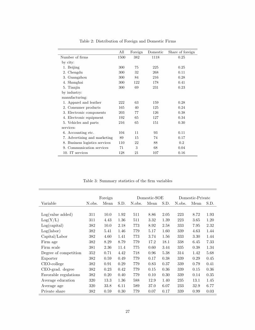
Table 2: Distribution of Foreign and Domestic Firms

All Foreign Domestic Share of foreign

Number of firms 1500 382 1118 0.25

by city:

1. Beijing 300 75 225 0.25

2. Chengdu 300 32 268 0.11

3. Guangzhou 300 84 216 0.28

4. Shanghai 300 122 178 0.41

5. Tianjin 300 69 231 0.23

by industry:

manufacturing:

1. Apparel and leather 222 63 159 0.28

2. Consumer products 165 40 125 0.24

3. Electronic components 203 77 126 0.38

4. Electronic equipment 192 65 127 0.34

5. Vehicles and parts 216 65 151 0.30

services:

6. Accounting etc. 104 11 93 0.11

7. Advertising and marketing 89 15 74 0.17

8. Business logistics services 110 22 88 0.2

9. Communication services 71 3 68 0.04

10. IT services 128 21 107 0.16

Table 3: Summary statistics of the firm variables

Foreign Domestic-SOE Domestic-PrivateVariable N.obs. Mean S.D. N.obs. Mean S.D. N.obs. Mean S.D.

Log(value added) 311 10.0 1.92 511 8.86 2.05 223 8.72 1.93Log(Y/L) 311 4.43 1.36 511 3.32 1.39 223 3.65 1.20Log(capital) 382 10.0 2.18 773 8.92 2.58 333 7.95 2.32Log(labor) 382 5.41 1.46 779 5.17 1.60 339 4.63 1.44Capital/Labor 382 4.60 1.41 773 3.74 1.56 333 3.30 1.44Firm age 382 8.29 8.79 779 17.2 18.1 338 6.45 7.33Firm scale 381 2.36 11.4 775 0.60 3.44 335 0.38 1.34Degree of competition 352 0.71 4.42 718 0.96 5.38 314 1.42 5.68Exporter 382 0.59 0.49 779 0.17 0.38 339 0.29 0.45CEO-college 382 0.91 0.29 779 0.83 0.37 339 0.79 0.41CEO-grad. degree 382 0.23 0.42 779 0.15 0.36 339 0.15 0.36Favorable regulations 382 0.20 0.40 779 0.10 0.30 339 0.14 0.35Average education 320 13.3 1.36 588 12.9 1.40 235 13.1 1.45Average age 320 33.8 6.11 589 37.0 6.07 233 32.9 6.77Private share 382 0.59 0.30 779 0.07 0.17 339 0.99 0.03

27

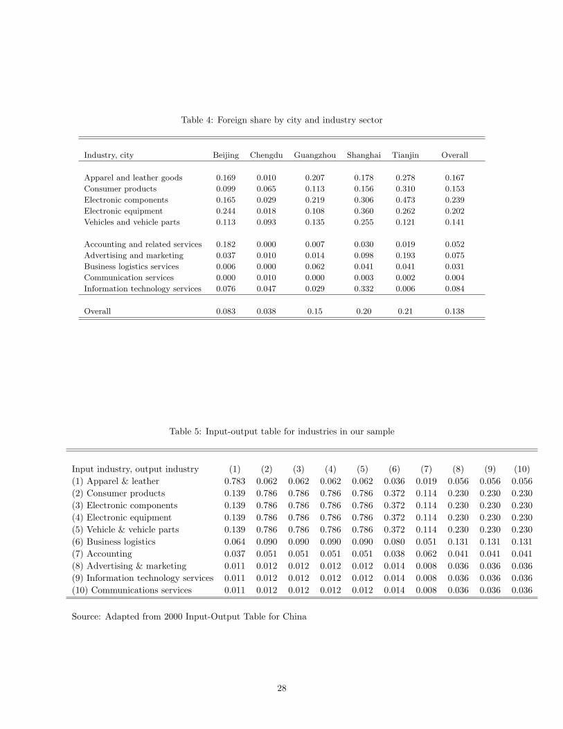
Table 4: Foreign share by city and industry sector

Industry, city Beijing Chengdu Guangzhou Shanghai Tianjin Overall

Apparel and leather goods 0.169 0.010 0.207 0.178 0.278 0.167

Consumer products 0.099 0.065 0.113 0.156 0.310 0.153

Electronic components 0.165 0.029 0.219 0.306 0.473 0.239

Electronic equipment 0.244 0.018 0.108 0.360 0.262 0.202

Vehicles and vehicle parts 0.113 0.093 0.135 0.255 0.121 0.141

Accounting and related services 0.182 0.000 0.007 0.030 0.019 0.052

Advertising and marketing 0.037 0.010 0.014 0.098 0.193 0.075

Business logistics services 0.006 0.000 0.062 0.041 0.041 0.031

Communication services 0.000 0.010 0.000 0.003 0.002 0.004

Information technology services 0.076 0.047 0.029 0.332 0.006 0.084

Overall 0.083 0.038 0.15 0.20 0.21 0.138

Table 5: Input-output table for industries in our sample

Input industry, output industry (1) (2) (3) (4) (5) (6) (7) (8) (9) (10)(1) Apparel & leather 0.783 0.062 0.062 0.062 0.062 0.036 0.019 0.056 0.056 0.056(2) Consumer products 0.139 0.786 0.786 0.786 0.786 0.372 0.114 0.230 0.230 0.230(3) Electronic components 0.139 0.786 0.786 0.786 0.786 0.372 0.114 0.230 0.230 0.230(4) Electronic equipment 0.139 0.786 0.786 0.786 0.786 0.372 0.114 0.230 0.230 0.230(5) Vehicle & vehicle parts 0.139 0.786 0.786 0.786 0.786 0.372 0.114 0.230 0.230 0.230(6) Business logistics 0.064 0.090 0.090 0.090 0.090 0.080 0.051 0.131 0.131 0.131(7) Accounting 0.037 0.051 0.051 0.051 0.051 0.038 0.062 0.041 0.041 0.041(8) Advertising & marketing 0.011 0.012 0.012 0.012 0.012 0.014 0.008 0.036 0.036 0.036(9) Information technology services 0.011 0.012 0.012 0.012 0.012 0.014 0.008 0.036 0.036 0.036(10) Communications services 0.011 0.012 0.012 0.012 0.012 0.014 0.008 0.036 0.036 0.036

Source: Adapted from 2000 Input-Output Table for China

28

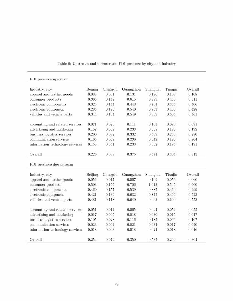
Table 6: Upstream and downstream FDI presence by city and industry

FDI presence upstream

Industry, city Beijing Chengdu Guangzhou Shanghai Tianjin Overallapparel and leather goods 0.088 0.031 0.131 0.196 0.108 0.108consumer products 0.365 0.142 0.615 0.889 0.450 0.511electronic components 0.323 0.144 0.448 0.761 0.365 0.406electronic equipment 0.283 0.126 0.540 0.753 0.400 0.428vehicles and vehicle parts 0.344 0.104 0.549 0.839 0.505 0.461

accounting and related services 0.071 0.026 0.111 0.163 0.090 0.091advertising and marketing 0.157 0.052 0.233 0.338 0.193 0.192business logistics services 0.200 0.082 0.332 0.509 0.263 0.280communication services 0.163 0.052 0.236 0.342 0.195 0.204information technology services 0.158 0.051 0.233 0.332 0.195 0.191

Overall 0.226 0.088 0.375 0.571 0.304 0.313

FDI presence downstream

Industry, city Beijing Chengdu Guangzhou Shanghai Tianjin Overallapparel and leather goods 0.056 0.017 0.067 0.109 0.056 0.060consumer products 0.503 0.155 0.706 1.013 0.545 0.600electronic components 0.460 0.157 0.539 0.885 0.460 0.499electronic equipment 0.421 0.139 0.632 0.877 0.496 0.523vehicles and vehicle parts 0.481 0.118 0.640 0.963 0.600 0.553

accounting and related services 0.051 0.014 0.065 0.094 0.054 0.055advertising and marketing 0.017 0.005 0.018 0.030 0.015 0.017business logistics services 0.105 0.028 0.116 0.185 0.096 0.107communication services 0.023 0.004 0.021 0.034 0.017 0.020information technology services 0.018 0.003 0.018 0.024 0.018 0.016

Overall 0.254 0.079 0.350 0.537 0.299 0.304

29

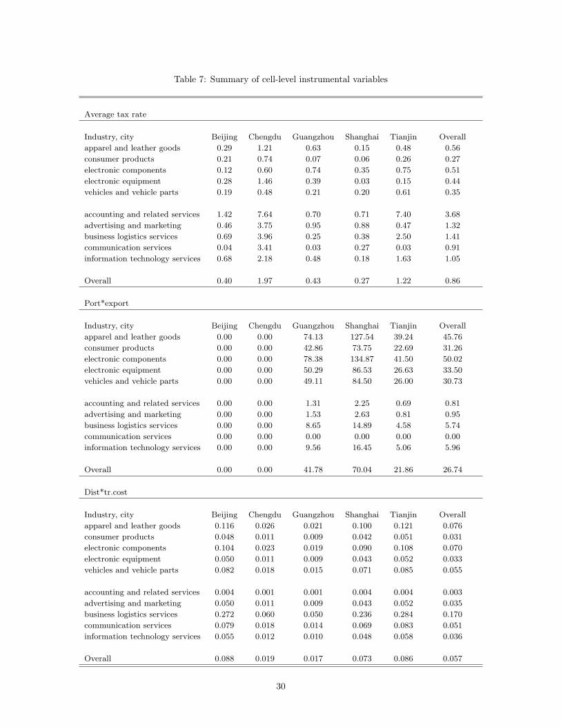
Table 7: Summary of cell-level instrumental variables

Average tax rate

Industry, city Beijing Chengdu Guangzhou Shanghai Tianjin Overall

apparel and leather goods 0.29 1.21 0.63 0.15 0.48 0.56

consumer products 0.21 0.74 0.07 0.06 0.26 0.27

electronic components 0.12 0.60 0.74 0.35 0.75 0.51

electronic equipment 0.28 1.46 0.39 0.03 0.15 0.44

vehicles and vehicle parts 0.19 0.48 0.21 0.20 0.61 0.35

accounting and related services 1.42 7.64 0.70 0.71 7.40 3.68

advertising and marketing 0.46 3.75 0.95 0.88 0.47 1.32

business logistics services 0.69 3.96 0.25 0.38 2.50 1.41

communication services 0.04 3.41 0.03 0.27 0.03 0.91

information technology services 0.68 2.18 0.48 0.18 1.63 1.05

Overall 0.40 1.97 0.43 0.27 1.22 0.86

Port*export

Industry, city Beijing Chengdu Guangzhou Shanghai Tianjin Overall

apparel and leather goods 0.00 0.00 74.13 127.54 39.24 45.76

consumer products 0.00 0.00 42.86 73.75 22.69 31.26

electronic components 0.00 0.00 78.38 134.87 41.50 50.02

electronic equipment 0.00 0.00 50.29 86.53 26.63 33.50

vehicles and vehicle parts 0.00 0.00 49.11 84.50 26.00 30.73

accounting and related services 0.00 0.00 1.31 2.25 0.69 0.81

advertising and marketing 0.00 0.00 1.53 2.63 0.81 0.95

business logistics services 0.00 0.00 8.65 14.89 4.58 5.74

communication services 0.00 0.00 0.00 0.00 0.00 0.00

information technology services 0.00 0.00 9.56 16.45 5.06 5.96

Overall 0.00 0.00 41.78 70.04 21.86 26.74

Dist*tr.cost

Industry, city Beijing Chengdu Guangzhou Shanghai Tianjin Overall

apparel and leather goods 0.116 0.026 0.021 0.100 0.121 0.076

consumer products 0.048 0.011 0.009 0.042 0.051 0.031

electronic components 0.104 0.023 0.019 0.090 0.108 0.070

electronic equipment 0.050 0.011 0.009 0.043 0.052 0.033

vehicles and vehicle parts 0.082 0.018 0.015 0.071 0.085 0.055

accounting and related services 0.004 0.001 0.001 0.004 0.004 0.003

advertising and marketing 0.050 0.011 0.009 0.043 0.052 0.035

business logistics services 0.272 0.060 0.050 0.236 0.284 0.170

communication services 0.079 0.018 0.014 0.069 0.083 0.051

information technology services 0.055 0.012 0.010 0.048 0.058 0.036

Overall 0.088 0.019 0.017 0.073 0.086 0.057

30

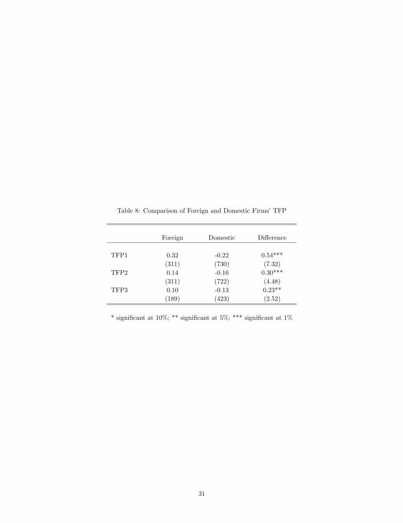
Table 8: Comparison of Foreign and Domestic Firms’ TFP

Foreign Domestic Difference

TFP1 0.32 -0.22 0.54***(311) (730) (7.32)

TFP2 0.14 -0.16 0.30***(311) (722) (4.48)

TFP3 0.10 -0.13 0.23**(189) (423) (2.52)

* significant at 10%; ** significant at 5%; *** significant at 1%

31

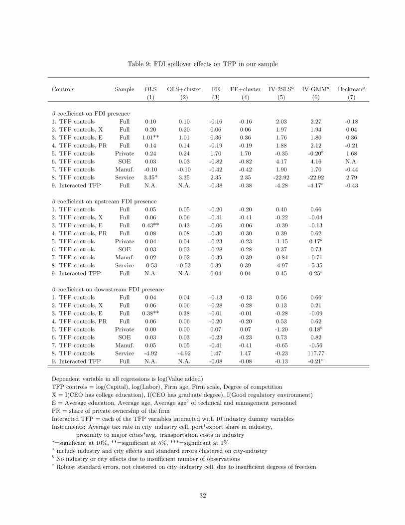
Table 9: FDI spillover effects on TFP in our sample

Controls Sample OLS OLS+cluster FE FE+cluster IV-2SLSa IV-GMMa Heckmana

(1) (2) (3) (4) (5) (6) (7)

β coefficient on FDI presence

1. TFP controls Full 0.10 0.10 -0.16 -0.16 2.03 2.27 -0.18

2. TFP controls, X Full 0.20 0.20 0.06 0.06 1.97 1.94 0.04

3. TFP controls, E Full 1.01** 1.01 0.36 0.36 1.76 1.80 0.36

4. TFP controls, PR Full 0.14 0.14 -0.19 -0.19 1.88 2.12 -0.21

5. TFP controls Private 0.24 0.24 1.70 1.70 -0.35 -0.20b 1.68

6. TFP controls SOE 0.03 0.03 -0.82 -0.82 4.17 4.16 N.A.

7. TFP controls Manuf. -0.10 -0.10 -0.42 -0.42 1.90 1.70 -0.44

8. TFP controls Service 3.35* 3.35 2.35 2.35 -22.92 -22.92 2.79

9. Interacted TFP Full N.A. N.A. -0.38 -0.38 -4.28 -4.17c -0.43

β coefficient on upstream FDI presence

1. TFP controls Full 0.05 0.05 -0.20 -0.20 0.40 0.66

2. TFP controls, X Full 0.06 0.06 -0.41 -0.41 -0.22 -0.04

3. TFP controls, E Full 0.43** 0.43 -0.06 -0.06 -0.39 -0.13

4. TFP controls, PR Full 0.08 0.08 -0.30 -0.30 0.39 0.62

5. TFP controls Private 0.04 0.04 -0.23 -0.23 -1.15 0.17b

6. TFP controls SOE 0.03 0.03 -0.28 -0.28 0.37 0.73

7. TFP controls Manuf. 0.02 0.02 -0.39 -0.39 -0.84 -0.71

8. TFP controls Service -0.53 -0.53 0.39 0.39 -4.97 -5.35

9. Interacted TFP Full N.A. N.A. 0.04 0.04 0.45 0.25c

β coefficient on downstream FDI presence

1. TFP controls Full 0.04 0.04 -0.13 -0.13 0.56 0.66

2. TFP controls, X Full 0.06 0.06 -0.28 -0.28 0.13 0.21

3. TFP controls, E Full 0.38** 0.38 -0.01 -0.01 -0.28 -0.09

4. TFP controls, PR Full 0.06 0.06 -0.20 -0.20 0.53 0.62

5. TFP controls Private 0.00 0.00 0.07 0.07 -1.20 0.18b

6. TFP controls SOE 0.03 0.03 -0.23 -0.23 0.73 0.82

7. TFP controls Manuf. 0.05 0.05 -0.41 -0.41 -0.65 -0.56

8. TFP controls Service -4.92 -4.92 1.47 1.47 -0.23 117.77

9. Interacted TFP Full N.A. N.A. -0.08 -0.08 -0.13 -0.21c

Dependent variable in all regressions is log(Value added)

TFP controls = log(Capital), log(Labor), Firm age, Firm scale, Degree of competition

X = I(CEO has college education), I(CEO has graduate degree), I(Good regulatory environment)

E = Average education, Average age, Average age2 of technical and management personnel

PR = share of private ownership of the firm

Interacted TFP = each of the TFP variables interacted with 10 industry dummy variables

Instruments: Average tax rate in city–industry cell, port*export share in industry,

proximity to major cities*avg. transportation costs in industry

*=significant at 10%, **=significant at 5%, ***=significant at 1%a include industry and city effects and standard errors clustered on city-industryb No industry or city effects due to insufficient number of observationsc Robust standard errors, not clustered on city–industry cell, due to insufficient degrees of freedom

32

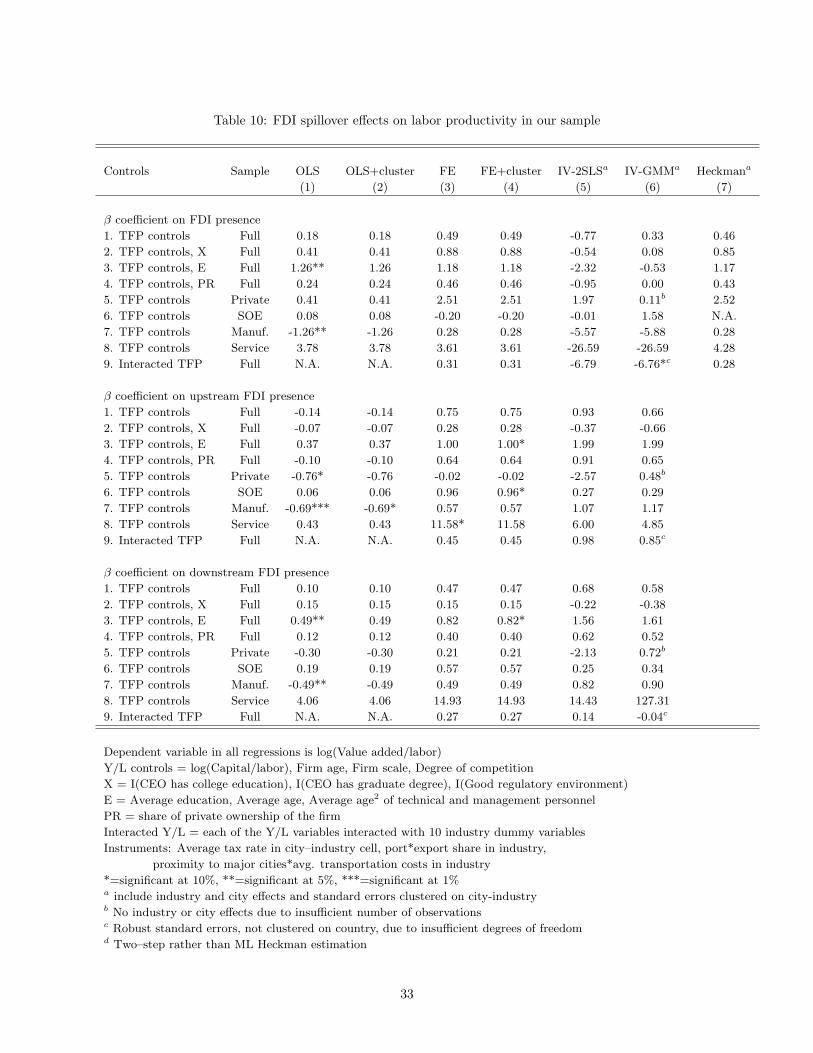
Table 10: FDI spillover effects on labor productivity in our sample

Controls Sample OLS OLS+cluster FE FE+cluster IV-2SLSa IV-GMMa Heckmana

(1) (2) (3) (4) (5) (6) (7)

β coefficient on FDI presence

1. TFP controls Full 0.18 0.18 0.49 0.49 -0.77 0.33 0.46

2. TFP controls, X Full 0.41 0.41 0.88 0.88 -0.54 0.08 0.85

3. TFP controls, E Full 1.26** 1.26 1.18 1.18 -2.32 -0.53 1.17

4. TFP controls, PR Full 0.24 0.24 0.46 0.46 -0.95 0.00 0.43

5. TFP controls Private 0.41 0.41 2.51 2.51 1.97 0.11b 2.52

6. TFP controls SOE 0.08 0.08 -0.20 -0.20 -0.01 1.58 N.A.

7. TFP controls Manuf. -1.26** -1.26 0.28 0.28 -5.57 -5.88 0.28

8. TFP controls Service 3.78 3.78 3.61 3.61 -26.59 -26.59 4.28

9. Interacted TFP Full N.A. N.A. 0.31 0.31 -6.79 -6.76*c 0.28

β coefficient on upstream FDI presence

1. TFP controls Full -0.14 -0.14 0.75 0.75 0.93 0.66

2. TFP controls, X Full -0.07 -0.07 0.28 0.28 -0.37 -0.66

3. TFP controls, E Full 0.37 0.37 1.00 1.00* 1.99 1.99

4. TFP controls, PR Full -0.10 -0.10 0.64 0.64 0.91 0.65

5. TFP controls Private -0.76* -0.76 -0.02 -0.02 -2.57 0.48b

6. TFP controls SOE 0.06 0.06 0.96 0.96* 0.27 0.29

7. TFP controls Manuf. -0.69*** -0.69* 0.57 0.57 1.07 1.17

8. TFP controls Service 0.43 0.43 11.58* 11.58 6.00 4.85

9. Interacted TFP Full N.A. N.A. 0.45 0.45 0.98 0.85c

β coefficient on downstream FDI presence

1. TFP controls Full 0.10 0.10 0.47 0.47 0.68 0.58

2. TFP controls, X Full 0.15 0.15 0.15 0.15 -0.22 -0.38

3. TFP controls, E Full 0.49** 0.49 0.82 0.82* 1.56 1.61

4. TFP controls, PR Full 0.12 0.12 0.40 0.40 0.62 0.52

5. TFP controls Private -0.30 -0.30 0.21 0.21 -2.13 0.72b

6. TFP controls SOE 0.19 0.19 0.57 0.57 0.25 0.34

7. TFP controls Manuf. -0.49** -0.49 0.49 0.49 0.82 0.90

8. TFP controls Service 4.06 4.06 14.93 14.93 14.43 127.31

9. Interacted TFP Full N.A. N.A. 0.27 0.27 0.14 -0.04c

Dependent variable in all regressions is log(Value added/labor)

Y/L controls = log(Capital/labor), Firm age, Firm scale, Degree of competition

X = I(CEO has college education), I(CEO has graduate degree), I(Good regulatory environment)

E = Average education, Average age, Average age2 of technical and management personnel

PR = share of private ownership of the firm

Interacted Y/L = each of the Y/L variables interacted with 10 industry dummy variables

Instruments: Average tax rate in city–industry cell, port*export share in industry,

proximity to major cities*avg. transportation costs in industry

*=significant at 10%, **=significant at 5%, ***=significant at 1%a include industry and city effects and standard errors clustered on city-industryb No industry or city effects due to insufficient number of observationsc Robust standard errors, not clustered on country, due to insufficient degrees of freedomd Two–step rather than ML Heckman estimation

33