ARE THE TWIN DEFICITS REALLY RELATED?

ARE THE TWIN DEFICITS REALLY RELATED? STEPHEN M. MILLER and FRANK S. RUSSEK*

The emergence of record current-account and fiscal deficits in the United States during the 1980s draws increasing attention to what has become known as the “twin deficit” problem. Conven- tional wisdom is that a shifi to larger government deficits entails a decline in government saving and results in larger trade deficits. Persistently large trade deficits are troublesome because they imply a transfer of wealth to foreigners and possibly a reduction in future generations’ living standards.

This paper examines whether post-World War II data for the United States reveal a long-run secular relationship between the trade deficit and the fiscal deficit. The focus is on the secular relationship since that is the one most relevant to long-run policy concerns. The authors employ three different statistical techniques: ( i ) a deterministic technique for separating the secular components from the cyclical components to derive secular measures of the twin deficits, (ii} a stochastic procedure to isolate the secular components, (iii) cointegration analysis to test for a long-run equilibrium relationship.

The authors conclude that, based on the first two approaches, evidence of a positive secular relationship between the twin deficits exists only under flexible exchange rates. This relationship appears quite strong-that is, a $I change in the fiscal deficit eventually lea& to roughly a $I change in the trade deficit. On the other hand, findings based on cointegration analysis indicate no long-run equilibrium relationship between the twin deficits. This latter finding, however, may reflect a low power of the relevant statistical tests stemming from the shortness of the sample period.

I. INTRODUCTION

The U.S. balance of trade shifted dramatically from surpluses to large deficits during the 1980s. Persistently large trade deficits are troublesome

*Professor of Economics, University of Connecticut, Storrs, and Principal Analyst, Congres- sional Budget Office, Washington, D.C., respectively. Miller was a Principal Analyst at the Con- gressional Budget Office when this research was completed. An earlier version of this paper was presented at the Western Economic Association International 63rd Annual Conference, Los An- geles, July 2, 1988, in a session organized by Frank Russek. The authors thank Suzanne J. Cooper for valuable research assistance and Stephan S. Thurman for the use of his international trade model. The authors also acknowledge the helpful comments of two anonymous referees and of coeditor Alejandra Cox Edwards. The views expressed in this paper are the authors’ and do not necessarily reflect those of the Congressional Budget Office or its staff.

91 Contemporary Policy Issues Vol. VII. October 1989

92 CONTEMPORARY POLICY ISSUES

due to the associated transfer of wealth to foreigners and the burden that this imposes on future generations. Many observers attribute a significant portion of this deterioration in the trade balance to the emergence of record federal fiscal deficits. The relationship between these two deficits is popularly termed the “twin deficit” problem.

The main purpose of this paper is to explore whether post-World War I1 data reveal a positive long-run or secular relationship between the trade deficit and the fiscal deficit. Conventional wisdom suggests that the currently large U.S. trade deficit resulted largely from the shift to larger fiscal deficits during the Reagan administration. Cyclical economic activity implies a negative relationship: Growing nominal GNP reduces the fiscal deficit but ex- pands the trade deficit, other things constant. Thus, to test the conventional wisdom, the focus here is on the secular movements in the twin deficits so as to eliminate the effect of cyclical events.

The approach of this paper uses several different statistical techniques to isolate and then estimate the relationship between secular movements in the twin deficits. It also applies a relatively new technique, cointegration analysis, to test for a long-run or equilibrium relationship. The methodology here differs from the more common practice of testing for a long-run relationship by including cyclical control variables in regression equations. In crude terms, this methodology dovetails with that used in studies testing for a short-run relationship between trend-adjusted movements in variables.

Section I1 overviews the post-World War I1 patterns of U.S. fiscal and trade deficits, especially those during the 1980s when the twin deficit question emerged as a widely discussed public policy issue.

Section I11 outlines some basic analytical views about the twin deficit relationship in open-economy macroeconomic models. It employs the saving-investment identity in focusing the discussion.

Section IV reviews the empirical literature bearing directly or indirectly on the twin deficit relationship. It considers some indirect evidence-i.e., how fiscal deficits affect determinants of the trade deficit-since relatively few studies examine the direct relationship.

Section V presents empirical results of three different but related approaches. First, a trend-cycle decomposition of the fiscal deficit is constructed by following the procedures that the Commerce Department developed to separate the fiscal deficit into its structural and cyclical parts. A similar procedure described below is applied to the trade deficit. Then a test is conducted for a significant relationship between the two cyclically adjusted deficit measures.

Second, a stochastic decomposition technique is used to generate secular components of the twin deficits for regression analysis. Recent advances in econometric methodology and practice have produced several new techniques for extracting secular components from observed time series. One such new technique is adopted here.

MILLER and RUSSEK: ARE THE TWIN DEFICITS REALLY RELATED? 93

Finally, cointegration analysis is used to test for a long-run equilibrium relationship between the twin deficits. The cointegration technique requires no trend-cycle decomposition. Instead, it relies soley on the raw data. None- theless, the technique purports to focus on low-frequency (long-run) relationships.

The conclusion of the analysis is that deterministic and stochastic measures of the secular components reveal a consistent long-run relationship between the twin deficits only under flexible exchange rates. This relationship is positive and strong: A $1 increase in the fiscal deficit associates with about a $1 increase in the trade deficit. By contrast, cointegration analysis suggests no secular relationship. This provides a cautionary note on the previous conclusion.

II. HISTORICAL DATA ON TRADE AND FISCAL DEFICITS

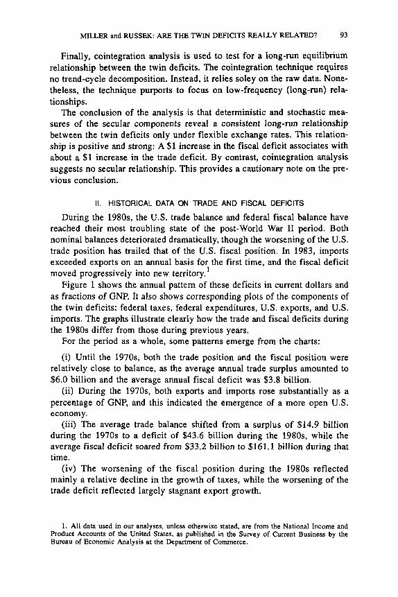
During the 1980s, the U.S. trade balance and federal fiscal balance have reached their most troubling state of the post-World War I1 period. Both nominal balances deteriorated dramatically, though the worsening of the U.S. trade position has trailed that of the U.S. fiscal position. In 1983, imports exceeded exports on an annual basis for the first time, and the fiscal deficit

1 moved progressively into new territory. Figure 1 shows the annual pattern of these deficits in current dollars and

as fractions of GNP. It also shows corresponding plots of the components of the twin deficits: federal taxes, federal expenditures, U.S. exports, and U.S. imports. The graphs illustrate clearly how the trade and fiscal deficits during the 1980s differ from those during previous years.

For the period as a whole, some patterns emerge from the charts:

(i) Until the 1970s, both the trade position and the fiscal position were relatively close to balance, as the average annual trade surplus amounted to $6.0 billion and the average annual fiscal deficit was $3.8 billion.

(ii) During the 1970s, both exports and imports rose substantially as a percentage of GNP, and this indicated the emergence of a more open U.S. economy.

(iii) The average trade balance shifted from a surplus of $14.9 billion during the 1970s to a deficit of $43.6 billion during the 1980s, while the average fiscal deficit soared from $33.2 billion to $161.1 billion during that time.

(iv) The worsening of the fiscal position during the 1980s reflected mainly a relative decline in the growth of taxes, while the worsening of the trade deficit reflected largely stagnant export growth.

1. All data used in our analyses, unless otherwise stated, are from the National Income and Product Accounts of the United States, as published in the Survey of Current Business by the Bureau of Economic Analysis at the Department of Commerce.

94

500 - 4 0 0 - 300-

200 -

100 -

CONTEMPORARY POLICY ISSUES

FIGURE 1 Trade and Federal Surpluses During the Post-World War I1 Period

U.S. Federal and Trade Surpluses 5 0

Trade Surplus L - -. ’ -d--/- .\-I !

Federal Surplus

(u

0 -100-

i -150-

-200 -

-250 -

m

l l l l l l l l l l l l l L 46 49 52 55 58 61 64 67 70 73 76 79 02 85 e

u.3. reaera Keceipts ma hxpenaitures 1200

1000 Expenditures /

1 1 1 1 I I I I I 1 I I 1 52 55 58 61 64 67 70 73 7 6 79 82 85 8

U.S. Exports and Imports 700,

I

/

MILLER and RUSSEK: ARE THE TWIN DEFICITS REALLY RELATED'? 95

FIGURE 1 (continued)

US. Federal and Trade Surpluses

-4 - l l l l l l l l f l l l l

4 6 ;9 52 5 5 5 8 61 6 4 67 7 0 73 76 79 82 85 e -6 -

U.S. Federal Receipts and Expenditures - 26 Expend i tums

U.S. Exports and Imports


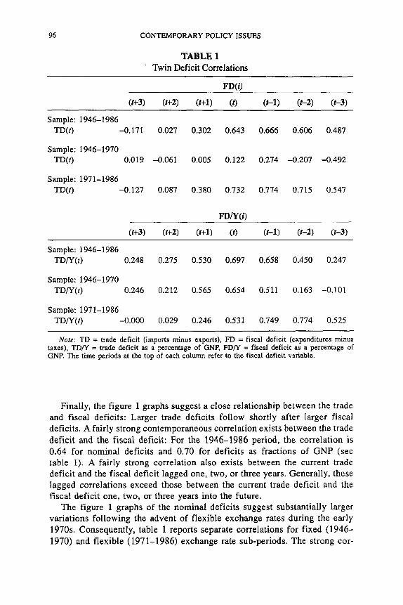
TABLE 1 Twin Deficit Correlations

(t+3) (t+2) (t+l) ( t ) (t-1) (t-2) (t-3)

Sample: 1946-1986 TD(t) -0.171 0.027 0.302 0.643 0.666 0.606 0.487

Sample: 1946-1970 TD(t) 0.019 -0.061 0.005 0.122 0.274 -0.207 -0.492

Sample: 1971-1986 TD(t) -0.127 0.087 0.380 0.732 0.774 0.715 0.547

FD/Y (i)

(t+3) (t+2) (t+l) (t) (t-1) (t-2) (t-3)

Sample: 1946-1986 TDTY(t) 0.248 0.275 0.530 0.697 0.658 0.450 0.247

Sample: 1946-1970 TD/Y(t) 0.246 0.212 0.565 0.654 0.511 0.163 -0.101

Sample: 1971-1986 TDTY(t) -0.000 0.029 0.246 0.531 0.749 0.774 0.525

~~ ~~

Note: TD = trade deficit (imports minus exports), FD = fiscal deficit (expenditures minus taxes), TD/Y = trade deficit as a percentage of GNP, FD/Y = fiscal deficit as a percentage of GNP. The time periods at the top of each column refer to the fiscal deficit variable.

Finally, the figure 1 graphs suggest a close relationship between the trade and fiscal deficits: Larger trade deficits follow shortly after larger fiscal deficits. A fairly strong contemporaneous correlation exists between the trade deficit and the fiscal deficit: For the 1946-1986 period, the correlation is 0.64 for nominal deficits and 0.70 for deficits as fractions of GNP (see table 1). A fairly strong correlation also exists between the current trade deficit and the fiscal deficit lagged one, two, or three years. Generally, these lagged correlations exceed those between the current trade deficit and the fiscal deficit one, two, or three years into the future.

The figure 1 graphs of the nominal deficits suggest substantially larger variations following the advent of flexible exchange rates during the early 1970s. Consequently, table 1 reports separate correlations for fixed (1946- 1970) and flexible (1971-1986) exchange rate sub-periods. The strong cor-


relations between the trade deficit and the lagged fiscal deficits continue under flexible exchange rates both for nominal deficits and for deficits as fractions of GNP. During fixed exchange rates, the correlations are weak for nominal deficits and for deficits as a fraction of GNP beyond a one-year lag. These correlations are not sufficient evidence for determining the direction of causality, but they generally support the common view that larger fiscal deficits lead to larger trade deficits over time-rather than the other way around. Such a commonly held view motivates the twin deficit analysis in Bernheim (1987) and Summers (1986b).

111. ANALYTIC FRAMEWORK

In one way or another, most open-economy macroeconomic models reflect the pioneering work of Mundell (1962, 1963) and Fleming (1963), which essentially extended the Keynesian model by introducing the external sector. In the Mundell-Fleming framework, the effect of fiscal policy depends on various factors-particularly the exchange rate regime.2 More specifically, under fixed rates, fiscal stimulus generates higher real income or prices, and this worsens the trade deficit. Under flexible rates, fiscal stimulus also worsens the trade deficit through appreciation of the currency. Thus, in both cases, the relationship between the trade deficit and the fiscal deficit is positive.

One can base a general view of the open macroeconomy on the saving- investment identity and how its components respond to exogenous economic shocksa3

The saving-investment identity is

(1) I = SH + SB + SG + SF

where I = investment net of depreciation, SH = household saving, SB = net business saving, SG = government saving (taxes minus spending), and SF = foreign saving (trade deficit with a negative sign).

A policy-induced increase in the fiscal deficit causes SG to fall exoge- nously. If one considers the saving-investment identity as an equilibrium

2. Other important factors include the degree of capital mobility and the size of the country. The literature often assumes high capital mobility and a country too small to affect world interest rates. To the extent that these conditions are not satisfied, the short-run linkages are weakened.

3. Other approaches are possible. First, a partial equilibrium view specifies the trade deficit as a function of several determinants-e.g., real GNP and the terms of trade-and examines how fiscal deficits affect the determinants of the trade deficit. In our review of the empirical evidence, the indirect evidence indicates how fiscal deficits affect the determinants of the trade deficit. Second, because we focus on the secular relationship between the twin deficits, an open-economy portfolio-balance growth model may be most appropriate. But the literature is somewhat deficient in this area. Several open-economy macroeconomic models examine long-run dynamics, but few models are explicitly growth models. For exceptions, see Ribe and Beeman (1986) and Turnovsky (1977).


condition, then such a decrease in SG must induce either an increase in SH + SB + SF or a decrease in I. An offsetting increase in private saving is prob- able only to the extent that individuals are Ricardian, taxes are lump sum, and government spending is a good substitute for private spending. If savers are not Ricardian, and if these other conditions are not met, then the fall in SG is associated with a fall in I, a rise in SF, or both. (For arguments sug- gesting that households adjust their savings in response to a shift in government saving, see Bailey, 1971, 1972; David and Scadding, 1974; Barro, 1974.)

The response of I and SF to a larger fiscal deficit depends on the degree of capital mobility, which may have increased under flexible exchange rates. If capital is highly mobile, then the domestic interest rate responds little to fiscal stimulus-thus not reducing investment-since foreign funds quickly offset the drain on domestic saving that the larger fiscal deficit generates. (This assumes that the policy change itself does not affect world interest rates directly.) These capital inflows, however, put upward pressure on the real exchange rate, either through a rising nominal exchange rate (under flexible rates) or a rising domestic price level (under fixed rates at capacity income). Because of exchange rate appreciation, the increase in the fiscal deficit crowds out net exports? The fiscal multiplier essentially is nil-the standard Mundell-Fleming conclusion. (A limitation of the Mundell-Fleming model is that it lacks an intertemporal budget constraint. This constraint potentially limits the persistence of fiscal and trade deficits. See Frankel and Razin, 1987.)

IV. REVIEW OF THE EMPIRICAL LITERATURE

Empirical conclusions about the twin deficit relationship must be based partly on indirect evidence since few studies examine this relationship directly. The effects of fiscal deficits on interest rates, exchange rates, and other proximate determinants of the trade deficit have been examined in various degrees of detail through both single-equation regressions and simulations of large-scale open economy macroeconometric models. These studies’ findings provide indirect and supplemental evidence about the twin deficit relationship.

A. Direct Evidence Apparently, little direct empirical evidence exists on the twin deficit re-

lationship based on regression analysis. Most such evidence comes from

4. A coordinated increase in fiscal deficits across countries raises world interest rates in tandem-Le.. differentials do not change. At capacity levels of real income, rising interest rates cause investment in each country to be crowded out. Then the fiscal deficit and investment in each country are negatively correlated. No correlation exists between the fiscal deficit and the trade deficit since the latter does not change.


large-scale model simulations. Generally, these latter studies contain more in-depth analysis of the issue, but often the focus is on post-1980 events providing only a limited basis for drawing long-run conclusions.

Single-Equation Regressions Milne (1977), in her study of 38 countries using annual data from 1960

to 1975, provides some statistical support for the fiscal approach to the balance of payments. The approach stresses the importance of the fiscal deficit in determining the trade deficit. (For a discussion of the fiscal approach to the balance of payments, see Bartoli, 1988.) In roughly half of the countries examined, Milne finds a positive and statistically significant ordinary least-square (OLS) relationship between the trade deficit and the fiscal deficit. She emphasizes that if the fiscal variable has a coefficient not significantly different from 1.00, then the fiscal deficit has no effect on private saving or investment. (For the United States, Milne finds no significant relationship.)

Another strand of empirical evidence apparently casts doubt on a one-to- one correspondence between the twin deficits. Several researchers (e.g., Feldstein and Horioka, 1980; Feldstein, 1983) observe a high positive correlation between national saving rates and domestic investment rates. Their findings question accepted views regarding the degree of international capital mobility. If international capital is highly mobile, then little reason exists for countries with high saving rates to necessarily have high investment rates, and vice versa. World saving should flow from countries with low interest rates to countries with high ones, so as to finance capital accumulation in the most productive economies. Consequently, the empirical regularity of a high correlation between national saving rates and domestic investment rates apparently contradicts the assumption of integrated world financial markets.

Generally, econometric tests of the empirical regularity focus on the long run: Investigators attempt to remove business cycle elements by averaging the national saving rates and domestic investment rates over several years- e.g., a decade. Generally, the regressions include the averaged rates across a sample of developed countries, but some studies include developing countries as well.

Recently, Dooley et al. (1987) reexamine the empirical regularity by at- tempting to address many potential econometric problems. They conclude that the finding of a strong positive correlation remains quite robust across numerous econometric tests. More recently, however, Miller (1988b) finds that national saving rates and domestic investment rates in the United States are not cointegrated under flexible exchange rates.

The empirical regularity between national saving and domestic investment may appear to have implications for the relationship between the twin deficits. If the government saving rate and the national saving rate are highly correlated-as several authors (e.g., Friedman, 197 1) have demonstrated-


then one might infer a fairly low correlation between the twin deficits when a fairly high correlation exists between national saving and domestic investment. However, the fairly strong correlation between the twin deficits reported in table 1 demonstrates that such an intuitive inference is invalid. Such an inference is based on raw correlations alone and fails to consider the relative variability of the variables determining the weights in the precise computations.

Summers (1986b) examines the effect of fiscal deficits on the composition of output using annual U.S. data from 1950 to 1985. He scales the twin deficits by GNP and includes cyclical control variables, His findings suggest that for the period as a whole, a $1 increase in the (total government) fiscal deficit increases the current-account deficit by 25 cents. Summers speculates that the effect may be larger for the more recent flexible exchange rate period.

In another recent study, Bernheim (1987) examines the historical relationship between the twin deficits using annual OECD data from 1960 to 1984 for the United States and five of its major trading partners. He employs OLS regressions of the current-account deficit on the contemporaneous (total government) fiscal deficit, a distributed lag of fiscal deficits, and real GNP growth rates as cyclical control variables. (The deficit variables are scaled by GNP.)’ Bernheim concludes that the fiscal deficit explains one-third of the current-account deficit in the United States. Findings of a significant relationship also hold for Canada, West Germany, the United Kingdom, and Mexico. For Japan, however, no significant relationship emerges.

Large-Scale Model Simulations. The magnitude of recent U.S. current-account deficits has produced a

growing literature examining its causes. One element of this research activity focuses on large-scale open-economy model simulations. In a summary of some simulation results, Hooper and Mann (1987) state that approximately two-thirds of the worsening of current-account deficits during 1982-1985 is due to fiscal policy actions-expansion at home and contraction abroad-and that domestic fiscal policy possesses the larger effect. Furthermore, the simulation results suggest that monetary policy, on average, fails to help explain the growth of current-account deficits. 6

5. Bernheim (1987) assumes that fiscal deficits cause trade deficits rather than the converse. A fiscal policy reaction function such as that described in Summers (1986a) reverses this direction of causality, or at least makes it bi-directional. We examine the causality issue in the next section.

6. Monetary policy has two effects working against each other. Expansionary monetary policy lowers interest rates and raises nominal income. Lower interest rates generate less (more) net capital inflow (outflow) and thus place downward pressure on the exchange rate and improve the trade balance. Higher nominal income stimulates imports and thus worsens the trade balance.


Sachs and Roubini (1987) provide simulation results based on a multi- country, rational expectations, general equilibrium model. They find that for the 1981-1985 period, a $1 increase in the U.S. fiscal deficit causes a worsening of the trade balance by 30 cents.

Several other more recent studies use large-scale open-economy macroeconomic models to simulate the future current-account effects of a permanent reduction in the fiscal deficit (see Bryant et al., 1988; Mason et al., 1988). Generally, these studies’ findings suggest that a $1 decrease in the fiscal deficit would cause a reduction of roughly 40 cents in the current account by the mid-1990s. (These findings are reviewed in more detail and others are presented in a recently published report by the Congressional Budget Office, August 1989.)

B. Indirect Evidence A large empirical literature offers indirect evidence on the twin deficit

relationship. Studies examine the effects of fiscal deficits on real income, the price level, interest rates, and the exchange rate. As in most empirical research, however, the conclusions reached in different studies often contra- dict one another. (For example, the effects of fiscal deficits on interest rates (CBO Staff Working Paper, 1989; Barth et al., 1984-1985) and on exchange rates (Feldstein, 1986; Evans, 1986) have not been settled.) Moreover, these conclusions may not apply to the question of a secular relationship between the twin deficits. (A longer version of this paper provides a discussion of the indirect linkages and citations to the relevant literature.)

V. EMPIRICAL RESULTS

The statistical analysis here focuses on the secular relationship between the twin deficits since this relationship is most relevant to long-run issues of policy concern such as the growth of external debt and the formation of domestic capital. First, the raw unfiltered data are examined as a benchmark and deterministic estimates of the secular deficits are used to assess the long-run relationship. Second, secular deficits derived from a stochastic method of secular-cyclical decomposition are considered. Finally, the long- run twin deficit relationship is examined by using cointegration analysis.

A. Actual (Unfiltered) Data Standard theoretical frameworks for policy analysis generally assume that

fiscal deficits are exogenous and that trade deficits are endogenous. Bernheim (1987) and Summers (1986b), for example, assume this in their empirical work. But, as Summers (1986a) observes, a fiscal policy reaction function that responds to trade deficits suggests reverse causality between the twin deficits.


Table 2 presents results of standard Granger causality tests to check the direction of temporal causality for periods of fixed and flexible exchange rates with 4, 8, and 12 lags of the nominal deficit and of deficits as fractions of GNP. (The correlation findings in table 1 suggest a possible break in the twin deficit relationship between fixed exchange rates and flexible exchange rates. Thus, the analysis here considers the two sub-periods ~eparately.)~ The F-statistics in table 2 suggest that fiscal deficits generally-but not uni- formly-lead trade deficits, and support for reverse causation is not over- whelming. The Bernheim (1987) and Summers (1986b) approach of regressing the trade deficit on current and lagged fiscal deficits appears reasonable. Thus, the analysis here follows their lead. (See Conway et al., 1984, who argue against the use of causality tests.)

Table 3 reports the findings of regressing the trade deficit on fiscal deficits with 0 and 12 lags. The 12 lags allow for three years of adjustment to changes in the fiscal deficit. (Because of space limitations, the results for 4 and 8 lags are not shown.) During fixed exchange rates (1946:l-1971:2), the sum of the coefficients on the current and lagged nominal fiscal deficits is significant but negative (equation lb) while the coefficient on the contemporaneous deficit is not significant (equation la). But when the deficits are scaled by GNP, the relationship is significantly positive in equations 3a and 3b. During flexible exchange rates (197 1:3-1987:2), the coefficients are positive and significant in all cases.

These findings are broadly consistent with the correlation results shown in table 1. In that table, a high correlation exists between all the trade and the contemporaneous and lagged fiscal deficit measures during flexible exchange rates. A high correlation also exists between all the trade and the contemporaneous and one-year lagged deficit-GNP ratios during fixed exchange rates. In the case of nominal deficits during fixed rates, however, even the contemporaneous correlation is low (0.122).

Most regressions in the upper part of each half of table 3 have an adjusted R2 larger than the Durbin-Watson statistic. Granger and Newbold (1974) argue that in such circumstances, the regression results may be spurious due

8

7. The nominal trade balance provides information different from that of the real trade balance, which focuses on the strength of the trade-oriented part of the economy. Generally, large nominal trade deficits mean large current-account deficits that must be financed by borrowing from abroad. A continuous buildup of foreign debt from years of large current-account deficits may be taken as a signal of weakness by the world foreign exchange and capital markets, and this may lead to reduced investor confidence. Moreover, to the extent that such borrowing finances domestic consumption rather than investment, less growth will occur in the capital stock and future living standards will decline. Edward M. Gramlich (1987) discusses the importance of the nominal trade deficit from a policy perspective. The nominal trade deficit often is scaled by GNP so as to take into account a country’s ability to finance its debt.

8. The results essentially are unchanged when contemporaneous and lagged money supply variables are included. Such a result supports the observation by Sachs and Roubini (1987, p. 30) that monetary policy has little effect on the trade deficit.


TABLE 2 Granger Causality Tests for the Twin Deficits

Nominal NominaYGNP

4 Lags 8 Lags 12 Lags 4 Lags 8Lags 12Lags

Sample: 1946:l-1971:2 FD Equation 1.495 0.908 1.055 1.734 2.538* 1.520

TD Equation 4.572* 3.384* 3.165* 1.387 4.006* 5.089*

Sample: 197 1 : 3- 1987 :3 FD Equation 1.016 1.281 1.252 1.316 2.564* 1.545

TD Equation 1.565 1.934** 1.822** 0.333 1.267 1.295

Note: The equations are of the following form: n n

D x ~ = UIJ + C UA Dxt-i + C Uyi Dyr-1 + Ut, i=l i-1

where x and y are FD and TD and vice-versa, Dx is the first difference of x, n takes on values 4, 8, and 12, and ut is a stationary random error. The F-statistics reported are for the joint significance of ayis.

*Significant at the 5 percent level. **Significant at the 10 percent level.

9 to non-stationary data. They suggest employing first-differenced regressions so as to test the robustness of the findings. (See also Plosser and Schwert, 1978. Barth et al., 1986, provide a practical example of this problem for questions of federal debt and private capital formation.) Another more recent approach is to apply cointegration tests, as is done below.

The equations in the lower portion of each half of table 3 are the first-differenced counterparts to those in the upper portion of each half of the table. The coefficients on the fiscal deficit are not statistically significant,

9. If non-stationary data are used, then the standard &statistics may be misleading. Based on augmented Dickey-Fuller tests, one can reject non-stationarity at the 5 percent level except for the nominal trade deficit during fixed exchange rates (see first two columns of table 8). But one cannot reject non-stationarity in any case under flexible rates. Regarding the first differences of all variables except the nominal trade deficit, one can reject non-stationarity under flexible rates. Nevertheless, coefficient estimates as well as autocorrelation and partial autocorrelation functions suggest that the first difference of the nominal trade deficit under flexible exchange rates also is stationary.


TABLE 3 Regressions Based cn Unfiltered Data: Fixed (1946:l-1971:2) and

Flexible (1971:3-1987:2) Exchange Rates

Equation Dependent Number Variable Intercept FD FDL R2/DW

la

l b

2a

2b

5a

5b

6a

6b

Equation Number

TD 1

TD 1

TD2

TD2

TD 1

TD 1

TD2

TD2

Dependent Variable

Undifferenced Data -6.08 0.20

(20.7) (0.5) -5.59 -

(21.8) - -32.04 0.45

(8.0) -47.85 (13.6) -

- (5.1)

First-Differenced Data 0.02 -0.01 (0.1)

-0.03 (0.4) -

1.86 0.06 (1.5) (0.09)

Intercept FDY

- 0.85

(22.6)

FDYL

-0.01 0.20 0.31 0.25 0.50 0.14 0.95 0.48

-0.01 1.75 0.25 2.20

-0.00 1.98 0.30 2.41

R'IDW

Undifferenced Data 3a TDlY -1.32 0.26

(14.0) (6.0) 3b

4a TD2Y -1.22 0.38

4b

- 0.26 - 0.27

TDlY -1.06 - 0.23 0.44 - (4.7) 0.30

- 0.23 - 0.18

0.91 - (20.0) 0.74

(23.7)

(4.4) TD2Y -2.88 - 1.06

First-Differenced Data

(4.3)

(17.6)

-0.00 - -0.01 - 1.75

7a TDlY 0.03 (0.0)

7b TDlY 0.01 - 0.18 0.39 (0.8)

(0.7) - (1.5) 1.97 -0.04 - -0.01

- 1.98 (0.7) TD2Y 0.01 - 0.77 0.20

- (2.8) 2.41

8a TD2Y 0.05 (1.1)

8b (0.2)

Nore: TDl = trade deficit (imports minus exports) during fixed-rate period, TD2 = trade deficit during flexiblerate period, TDlY = TDl as a percentage of GNF', TD2Y = TD2 as a percentage of GNP, FD = fiscal deficit (expenditures minus taxes) in either fixed- or flexible-rate period, FDL = current and 12 lagged values of FD, FDY = FD as a percentage of GNP, FDYL = current and 12 lagged values of FDY. Whenever the dependent variables are for the fixed- or flexible-rate period, so are the regressors. Absolute values of t-statistics are in parentheses, R2 is the adjusted coefficient of determination, and DW is the Dubin-Watson statistic.


except during flexible exchange rates with 12 lags. In this case, a $1 increase in the fiscal deficit eventually causes about a $1 increase in the trade deficit-a much larger estimate than those produced in previous studies. (As in the case of undifferenced data, including money stock variables does not alter these results.) Now consider the secular relationship between the twin deficits which has relevance for long-run issues of policy concern.

B. Deterministic Decomposition A model similar to that developed at the Commerce Department (see

DeLeeuw and Holloway, 1985) is used here to obtain an estimate of the secular component of the fiscal deficit based on non-stochastic decomposition. The model estimates cyclically adjusted federal taxes based on a time- trend measure of potential output. It also calculates cyclically adjusted federal spending based on a trend estimate of the non-accelerating inflation rate of unemployment (NAIRU).

Similarly, to estimate the secular component of exports and imports, a small-scale version of an international trade model (see Thurman and Foster, 1986) first developed at the Federal Reserve Board is used. This trade model is simulated with a time-trend estimate of U.S. potential output and with a measure of foreign potential output. The result is a cyclically adjusted measure of the trade deficit.

The upper part of each half of table 4 reports regressions using cyclically adjusted components of the twin deficits both with and without a 12-quarter lag on the fiscal deficit. The regressions cover only the flexible-rate period (1971:3-1987:2) due to the restricted time intervals of the models used to calculate these deficit measures. The fiscal variables' coefficients are positive and highly significant both for nominal deficits and for deficits scaled by U.S. potential GNP. In all cases, the coefficients are close to unity statistically.

The equations in the lower portion of each half of table 4 are the first- differenced counterparts to those in the upper portion of each half of the table." The results essentially are unaltered with differenced data. In, all but one case-equation 4a-the first-differenced regressions based on non-stochastic decomposition suggest a non-spurious and positive secular association between the twin deficits during flexible exchange rates. As in the case with unfiltered data, the 12-quarter cumulative effect implies that a $1 rise in the fiscal deficit causes about a $1 increase in the trade deficit.

10. Based on adjusted Dickey-Fuller tests as reported in the third and fourth columns of table 8, one cannot rejcct non-shtionarity for any variables in table 4 at the 5 percent level except for the first differences of the fiscal deficits. First differences of the trade deficits appear non- stationary by the adjusted Dickey-Fuller test, but coefficient estimates as well as autocorrelation and partial autocorrelation functions suggest otherwise.


TABLE 4 Regressions Based on Deterministic Decomposition: Flexible Exchange Rates

(1971:3-1987:2)

Equation Dependent Number Variable Intercept PFD PFDL R ~ I D W

Undifferenced Data

la PTD -36.98 0.84 - 0.84 (10.5) (18.5) - 0.59

l b PTD -42.2 - 1.02 0.95 (13.9) - (12.0) 0.94


3a PTD 1.97 0.21 - 0.08 (1.4) (2.5) - 2.24

3b PTD -0.18 - 1.07 0.14 (0.1) - (2.3) 2.58

Equation Dependent Number Variable Intercept PFDY PFDYL R?DW

Undifferenced Data

2a PTDY -1.82 0.94 (7.7) (8.5)

2b PTDY -2.12 - (7.9) -


4a PTDY 0.06 0.01 (1.3) (0.2)

(0.1) 4b PTDY 0.01 -

-

1.25 (7 5)

1.26 (2.2)

0.53 0.57

0.75 0.32

-0.02 2.07

0.11 2.41

Note: PTD = permanent trade deficit, FTDY = permanent trade deficit as a percentage of potential GNP, PFD = permanent fiscal deficit, PFDL = current and 12 lagged values of PFD, PFDY = PFD as a percentage of potential GNP,: PFfYL = current and 12 lagged values of PFDY. Absolute values of t-statistics are in parentheses, R is the adjusted coefficient of determination, and DW is the Durbin-Watson statistic.

MILLER and RLJSSEK: ARE THE TWIN DEFICITS REALLY RELATED’? 107

C. Stochastic Decomposition Currently, conflicting views exist over which is the most appropriate way

to stochastically extract the secular component of a time series. The dispute hinges on how much of the observed movement in macroeconomic time- series data represents secular adjustments rather than cyclical adjustments. Intuition suggests that secular movements are smooth and that cyclical adjustments reflect the bulk of the movement in the data. Such intuition underlies the commonly used time-trend methods of extracting secular components. On the other hand, stochastic methods of secular extraction introduce more movement into the secular component-and thus are less intuitive.

The procedure adopted here is one proposed by Beveridge and Nelson (198 1). Roughly, the Beveridge-Nelson technique places the major portion of the observed movement in a variable into the secular component. Thus, it is consistent with a real business cycle view of the world, as Nelson and Plosser (1982) discuss. (Watson, 1986, and Clark, 1987, separately proposed another technique placing more of a variable’s movement into the cyclical component .)

The Beveridge-Nelson technique is applied to nominal government expenditures and revenues, nominal exports and imports, and nominal GNP so as to be consistent with the deterministic decomposition procedures underlying table 4. Then the secular deficit series is constructed from their secular component parts. Table 5 reports the identified and estimated autoregressive integrated moving-average (ARIMA) models for each data series in the Beveridge-Nelson decomposition.

Tables 6 and 7 present regressions of the trade deficit on the fiscal deficit for fixed exchange rates and flexible exchange rates, respectively, based on secular components of the twin deficits derived with the Beveridge-Nelson (198 1) decomposition technique. Actual implementation follows the procedure suggested by Miller (1988a).

The table 6 results suggest no significantly positive relationship between the secular components of the twin deficits during fixed exchange rates. Even when one uses the level form of the data, no significantly positive relationship exists. And in one case, equation lb , the coefficient on the fiscal variable is significantly negative. During flexible exchange rates (table 7), evidence of a significant and positive non-spurious relationship does exist between the secular components of the nominal deficits. But the relationship may be spurious when the deficits are scaled by GNP.

As noted above, the Beveridge-Nelson decomposition technique causes the secular series to resemble the unfiltered data. Thus, that the findings in tables 6 and 7 conform roughly to the unfiltered data results in table 3 is not surprising. Neither set of results provides support for a non-spurious twin deficit relationship during fixed exchange rates. During flexible exchange


TABLE 5 ARIMA Models Underlying the Beveridge-Nelson Decomposition

Variable 1946:1-1971:2 1971:3-1987:2

Note: The variables are as follows: GF is federal government expenditure, TF is federal gov-

? h e (4) indicates an autoregressive term at lag 4 only. ernment revenue, EX is exports, and M is imports. The natural logarithm operator is In.

rates, on the other hand, both sets suggest a non-spurious positive relationship-at least for nominal deficits-when lags are included.

D. Cointegration Results Two or more non-stationary variables have a long-run equilibrium rela-

tionship if they are cointegrated, i.e., have a common trend (Engel and Granger, 1987). Testing for cointegration involves three steps. First, one determines the order of integration for each variable-that is, one assesses how many times the time series must be differenced so as to achieve stationarity. Second, one estimates cointegration equations with OLS for each set of non-stationary variables with the same orders of integration. Finally, one tests the residuals from the cointegration equations for non-stationarity. If non-stationarity is rejected, then the variables are cointegrated.

The first two columns of table 8 report the test statistics for determining the order of integration for each deficit both in nominal terms and relative to GNP (Fuller, 1976; Dickey-Fuller, 1979). During fixed exchange rates, one can reject non-stationarity at the 5 percent level for each series except the nominal trade deficit. Also, one can reject non-stationarity for the first difference of all series except the nominal trade deficit during flexible exchange rates. But during flexible exchange rates, one cannot reject non- stationarity for any variables in level form. Therefore, testing is restricted for cointegration of the twin deficits to the flexible-exchange-rate period, when both deficits satisfy the non-stationarity requirement.

The estimated cointegration regressions are the same as the OLS regressions reported in equations 2a and 4a of table 3. To determine whether the twin deficits are cointegrated, one can check the residuals from these


TABLE 6 Stochastic Decomposition Results, Beveridge-Nelson Technique :

Fixed Exchange Rates (1946:l-1971:2)

Equation Dependent Number Variable Intercept PFD PFDL R?DW

Undifferenced Data

l a PTD -6.16 0.00 (20.8) (0.1)

l b PTD -5.79 - (22.1) -


3a PTD 0.02 -0.00 (0.1) (0.2)

3b PTD -0.02 - - (0.2)

Equation Dependent Number Variable Intercept PFDY

- -0 .o 1 - 0.20

-0.22 0.26 (2.9) 0.25

- -0.01 - 1.90

0.17 0.22 (1.18) 2.27

PFDYL R2/DW

Undifferenced Data

2a PTDY -1.10 0.0 1 (18.0) (0.2)

2b PTDY -1 .oo - (24.6) -


4a PTDY 0.02 -0.04 (0.9) (1.9)

4b PTDY -0.00 - (0.1) -

0.02 (0.3)

0.14 (1.3)

-0.01 0.20

0.39 0.30

0.03 1.51

0.27 2.06

~~

Nore: PTD = permanent trade deficit, PTDY = permanent trade deficit as a percentage of potential GNP, PFD = permanent fiscal deficit, PFDL = current and 12 lagged values of PFD, PFDY = PFD as a percentage of potential GNP, PFDYL = current and 12 lagged values of PFDY. Absolute values at t-statistics are in parentheses, RZ is the adjusted coefficient of determination, and DW is the Durbin-Watson statistic.


TABLE 7 Stochastic Decomposition Results, Beveridge-Nelson Technique:

Flexible Exchange Rates (197 1:3-1987:2) ~ ~ ~~~

Equation Dependent Number Variable Intercept PFD PFDL RVDW

Undifferenced Data

la PTD -38.74 0.49 - 0.56 (6.3) (8.9) - 0.19

l b PTD -53.31 - 0.83 0.91 (14.4) - (20.9) 0.78


3a PTD 1.39 0.18 - 0.06 (0.9) (2.2) - 2.47

3b PTD -1.39 - 1.06 0.06 (0.6) - (2.5) 3.03

Equation Dependent Number Variable Intercept PFDY PFDYL RVDW

Undifferenced Data

2a PTDY -5.79 0.50 (6.1) (6.2)

2b PTDY -10.29 - (2 1.4) -

First-Differenced Data 4a PTDY 0.16 0.08

(0.8) (1.0)

(0.3) 4b PTDY 0.06 -

-

1.07 (24.1)

0.77 (1.92)

0.39 0.25

0.93 1.41

0.00 2.42

0.02 2.98

Note: PTD = permanent trade deficit, PTDY = permanent trade deficit as a percentage of potential GNP, PFD = permanent fiscal deficit, PFDL = current and 12 lagged values of PFD, PFDY = PFD as a percentage of potential GNP. PFDYL = current and 12 lagged values of PFDY. Absolute values of t-statistics are in parentheses, RZ is the adjusted coefficient of determination, and DW is the Durbin-Watson statistic.

MILLER and RUSSEK: ARE THE TWIN DEFICITS REALLY RELATED? 11 1

TABLE 8 Adjusted Dickey-Fuller Tests for Non-Stationarity

Beveridge- Actual Deterministic Nelson

Variable b i t(b 1 ) b i t(bl) b i 0 1 )

Fixed Rates 0.878 -2.76** n.a. n.a. 0.865 -2.93*

FD1 0.763 -3.39* n.a. n.a. 0.643 -3.64* TD 1

DTD 1 -0.156 -5.93* n.a. n.a. -0.216 -5.95* DFD 1 0.074 -4.92* n.a. n.a. -0.263 -5.03*

TD1 Y 0.875 -5.04* n.a. n.a. 0.739 -5.02* FDlY 0.806 -3.54* n.a. n.a. 0.614 -3.79*

DTD 1 Y -0.027 -6.40* n.a. n.a. 0.073 -5.41* DFD 1 Y 0.087 5.40* n.a. n.a. -0.380 -5.81*

Flexible Rates TD2 1.006 0.16 1.019 0.47 0.993 -0.15 FD2 0.942 -1.52 0.930 -1.51 0.942 -1.52

DTD2 0.322 -2.47 0.172 -2.63** 0.190 -2.47 DFD2 0.009 -3.09* 0.045 -2.24 0.009 -3.09*

TD2Y 0.991 -0.20 0.999 -0.02 0.983 -0.34 FD2Y 0.857 -2.10 0.866 -1.51 0.864 -2.11

DTD2Y 0.022 -3.35* -0.245 -3.95* -0.298 -3.52* DFD2Y -0.1 11 -3.49* -0.645 -3.75* -0.166 -3.52*

Nore: TD1 and TD2 are trade deficits with fixed and flexible exchange rates. FDl and FD2 are fiscal deficits with fixed and flexible exchange rates. All variables ending with Y are divided by GNP. Variables beginning with D are first differences, and In is the natural logarithm operator. The first two columns examine actual data, the third and fourth columns deterministic secular data, and the fourth and fifth columns Beveridge-Nelson secular data. The augmented Dickey- Fuller tests are based on the regression

4

XI= bo + bl X t - l + bl+i DXei + ~t i=l

where bis are parameters to estimate and ut is the random error. X takes on the values TDI, FDl, etc.

*Rejection of the null hypothesis of non-stationary time series or [(l-bl) = 01 at the 5 percent level.

**Rejection at the 10 percent level.


cointegration regressions for unit roots based on augmented Dickey-Fuller tests. The test statistics (-1.00 and -1.01) indicate that one cannot reject the null hypothesis of non-stationary residuals at the 5 percent level (-2.68 crit- ical value) for either the nominal deficits or the deficit-GNP ratios. In other words, the twin deficits have no long-run equilibrium relationship during flexible exchange rates." Given the shortness of the flexible-exchange-rate sample, however, the Dickey-Fuller and cointegration tests probably have low power.

These cointegration results provide a cautionary note for the previous findings in the case of flexible exchange rates. When unfiltered data are used, the twin deficit relationship first appears non-spurious except when the specification excludes lagged fiscal deficits. Deterministic decomposition suggests a non-spurious secular relationship in most cases. The Beveridge- Nelson decomposition also provides evidence of a non-spurious secular relationship-at least it does for nominal deficits. By contrast, cointegration analysis suggests that neither the nominal deficits nor the deficit-GNP ratios possess a common secular relationship.

What can one conclude from the apparent conflict? The absence of cointegration between the twin deficits may signal only omitted variables from the cointegration regression. Some higher-order system of three or more variables, including the twin deficits, may be cointegrated. For example, the twin deficits and the real exchange rate may be cointegrated even though the twin deficits alone are not.12 On the other hand, the results simply may reflect a low power of the cointegration test. A larger sample period may be needed so as to reconcile the conflicting results.

11. Estimated cointegration regressions of the fiscal deficit onto the trade deficit for nominal deficits and deficit-GNP ratios during flexible exchange rates yield higher cointegration coefficients than do those reported in table 3 (e.g., 1.11 and 0.63). But the residuals from these regressions also are non-stationary based on the augmented Dickey-Fuller test: The test statistics are -1.99 and -2.58.

12. As an experiment, we added sequentially the natural logarithms of the real exchange rate (e), U.S. real GNP (y), and a foreign real GNP index Of) to the cointegration regressions both for deficits and for deficits relative to GNP. Augmented Dickey-Fuller tests of the cointegration regression errors never reject the null hypothesis of non-stationarity (Engle and Yoo, 1987). Yet the autocorrelations and partial autocorrelations progressively suggest stationary errors as more variables are added. For the five-variable cointegration regression with the twin deficits measured relative to GNP. the autoconelation of the regression errors is 0.61 at lag 1 and then declines rapidly-approaching zero by lag 3. Does such an autocorrelation function indicate non-stationarity? We leave such a questions for future analysis. The estimated cointegration equation in the five-variable case for the scaled deficits is

TD2Y = -1.795 + 0.259 FD2Y + 0.007 In(e) + 0.354 InQ) - 0.233 he'). The augmented Dickey-Fuller statistic is -3.163, which cannot reject the null hypothesis that

the variables are not cointegrated. The Dickey-Fuller statistic of -3.646 also cannot reject this null hypothesis. The &statistics are not reported due to problems with interpreting them in the context of cointegration analysis (Engle and Granger, 1987).


VI. CONCLUSIONS

This paper has used alternative econometric techniques so as to test for a secular relationship between the U.S. trade deficit and the U.S. fiscal deficit. Findings based on deterministic calculations of the secular deficits and on the Beveridge-Nelson stochastic decomposition technique suggest a non-spurious relationship during the flexible-exchange-rate period-the fiscal deficit has roughly a one-to-one cumulative effect on the trade deficit following 12 quarters. Cointegration analysis, on the other hand, provides no support for a secular relationship. However, the power of the cointegration test probably is low. During the fixed-exchange rate period, regressions based on stochastically derived measures of the secular deficits imply no secular relationship.

REFERENCES

Bailey, M. J., National lncome and the Price Level, McGraw-Hill, New York, 1971. , “The Optimal Full-Employment Surplus,” Journal of Political Economy, July/August

1972, 649-661.

Barro, R. J., “Are Government Bonds Net Wealth?” Journal of Political Economy, November/ December 1974, 5-117.

Ba~th, J. R., G. Iden, and F. S. Russek, “Do Federal Deficits Really Matter?” Contemporary Policy Issues, Fall 1984, 79-95.

Barth, J. R., F. S. Russek, and G. H. K. Wang, “The Measurement and Significance of the Cyclically Adjusted Federal Budget and Debt,” Journal of Money, Credit and Banking, November 1986, 527-538.

Bartoli, G., “Fiscal Expansion and External Account Balance.” unpublished manuscript, International Monetary Fund, November 1988.

Bemheim, D., “Budget Deficits and the Balance of Trade,” in L. H. Summers, ed., Tar Policy and the Economy, National Bureau of Economic Research, 1987.

Beveridge, S., and C. R. Nelson, “A New Approach to Decomposition of Economic Time Series into Permanent and Transitory Components with Particular Attention to Measurement of the Business Cycle,” Journal of Monetary Economics, March 1981, 151-174.

Bryant, R. C., D. W. Henderson, G. Holtham, P. Hooper, and S. Symansky, eds., Empirical Macroeconomics for Interdependent Economics, The Brookings Institution, Washington, D.C., 1988.

Clark, P. K., “The Cyclical Component of U.S. Economic Activity,” Quarterly Journal of Economics, November 1987, 797-814.

Congressional Budget Office, “Deficits and Interest Rates: Theoretical Issues and Empirical Evidence,” staff working paper, Washington, D.C., January 1989.

, “Policies for Reducing the Current-Account Deficit,” Washington, D.C., August 1989.

Conway, R. K., P. A. V. B. Swamy, J. F. Yanagida, and P. von zur Muehlen, “The Impossibility of Causality Testing,” Agricultural Economics Research, Summer 1984, 1-19.

David, P. A., and J. L. Scadding, “Private Saving: Ultrarationality, Aggregation, and Dennison’s Law,” Journal of Political Economy, MarcNApril 1974, 225-249.

DeLeeuw, F., and T. M. Holloway, “The Measurement and Significance of the Cyclically Adjusted Federal Budget Deficit and Debt,” Journal of Money, Credit and Banking, May 1985, 232-242.

Dickey, D. A., and W. A. Fuller, “Distribution of Estimates of Autoregressive Time Series With Unit Roof” Journal of the American Statistical Association, June 1979, 427-43 1.


Dooley, M., I. Frankel, and D. J . Mathieson, “International Capital Mobility: What Do Saving-Investment Correlations Tell Us?” International Monetary Fund Staff Papers, September 1987, 503-530.

Engle, R. F., and C. W. J. Granger, “Co-Integration and Error Correction: Representation, Estimation, and Testing,” Econometrica. March 1987, 251-276.

Engle, R. F., and B. Sam Yoo, “Forecasting and Testing in Co-Integrated Systems,” Journal of Econometrics, May 1987, 143-159.

Evans, P., “Is the Dollar High Because of Large Budget Deficits?” Journal of Monetary Economics, November 1986, 227-249.

Feldstein, M., “Domestic Saving and International Capital Movements in the Long Run and the Short Run,” European Economic Review, MarcWApril 1983, 129-151.

, “The Budget Deficit and the Dollar,” NBER working paper No. 1898, Cambridge, Mass., April 1986.

Feldstein, M., and C. Horioke, “Domestic Saving and International Capital Mobility,” Economic Journal, June 1980, 314-329.

Fleming, J. M., “Domestic Financial Policies Under Fixed and Under Floating Exchange Rates,” International Monetary Fund Staff Papers, November 1962, 369-379.

Frenkel, J . A., and A. Razin, “The Mundell-Fleming Model a Quarter Century Later: A Unified Exposition,” International Monetary Fund Stafl Papers, December 1987, 567-620.

Friedman, B. M., “New Directions in the Relationship Between Public and Private Debt,” NBER working paper No. 2186, Cambridge, Mass., March 1987.

Fuller, W. A., Introduction to Statistical Time Series, Wiley, New York, 1976. Gramlich, E. M., “Statement of the Acting Director of the Congressional Budget Office Before

the Joint Economic Committee of the United States Congress,” November 5, 1987. Granger, C. W. J., and P. Newbold, “Spurious Regressions in Econometrics,” Journal of

Econometrics, July 1974, 111-120. Hooper, P., and C. L. Mann, “The U.S. External Deficit: Its Causes and Persistence,” prepared

for The US. Trade Deficit: Causes. Consequences, and Cures, a conference at the Federal Reserve Bank of St. Louis, October 1987.

Mason, P., S. Symansky, R. Haas, and M. Dodley, “Multimod: A Multi-Region Econometric Model,” International Monetary Fund, Washington, D.C., 1988.

Miller, S. M., “The Beveridge-Nelson Decomposition of Economic Time Series: Another Economical Computational Method,” Journal of Monetary Economics, January 1988(a), 14 1-142.

, “Are Saving and Investment Co-Integrated?” Economic Letters, 27: 1 , 1988(b),

Milne, E., “The Fiscal Approach to the Balance of Payments,” Economic Notes, November 1 , 1977, 89-107.

Mundell, R. A., “The Appropriate Use of Monetary and Fiscal Policy Under Fixed Exchange Rates,” International Monetary Fund Staff Papers, March 1962.

, “Capital Mobility and Stabilization Policy Under Fixed and Flexible Exchange Rates,” Canadian Journal of Economics and Political Science, November 1963, 475-485.

Nelson, C. R., and C. L. Plosser, “Trends and Ramdon Walks in Economic Time Series,” Journal of Monetary Economics, September 1982, 139-162.

Plosser, C. I . , and G. W. Schwert, “Money, Income, Sunspots: Measuring Economic Relationships and the Effects of Differencing,” Journal of Monetary Economics, November 1978,637-660.

Ribe, F. C., and W. J. Beeman, “The Monetary-Fiscal Mix in an Open Economy,” American Economic Review, May 1986, 209-213.

Sachs, J., and N. Roubini, “Sources of Macroeconomic Imbalances in the World Economy: A Simulation Approach.” NBER working paper No. 2339, Cambridge, Mass., August 1986.

3 1-34.


Summers, L. H., “Tax Policy and International Competitiveness,” Harvard Institute of Economic

, “Debt Problems and Macroeconomic Policies,” Harvard Institute of Economic

Thurman, S. S., and L. S. Foster, ”The Effects of Prolonged Exchange Rate Episodes on Trade

Tumovsky, S. J., Macroeconomic Analysis and Stabilization Policies, Cambridge University Press,

Watson, M. W., “Univariate Detrending Methods With Stochastic Trends,” Journal of Monetary

Research, discussion paper No. 1256, Cambridge, Mass., August 1986(a).

Research, discussion paper No. 1272, Cambridge, Mass., October 1986(b).

Equation Parameters,” unpublished, June 1986.

London, 1977.

Economics, July 1986, 49-75.

Documents

ARE THE TWIN DEFICITS REALLY RELATED?