Electronic copy available at: http://ssrn.com/abstract=2598955

ARE GROUPS BETTER PLANNERS THAN

INDIVIDUALS? AN EXPERIMENTAL ANALYSISI

Enrica Carbonea,∗, Gerardo Infanteb

aSeconda Universita di Napoli, Corso Gran Priorato di Malta n.1, 81043 Capua (CE),ITALY

bUniversity of East Anglia, Norwich Research Park, Norwich, NR4 7TJ, UK

Abstract

We present the results of an experiment comparing group and individual

planning in the domain of lifecycle consumption/saving decisions. Individual

decision making is compared to two group treatments, which differ based on

the presence of a rematching rule. We find that individuals and groups differ

in how they solve the intertemporal consumption problem, but not in how

they improve their consumption planning within a sequence. Individuals’

performance improves across sequences, groups without rematching perform

approximately the same, while groups with rematching do significantly worse.

Our main finding is that while groups perform better than individuals in

the first sequence, this difference seems to disappear in the second lifecycle.

Results show that in the second sequence groups in the rematching treatment

deviate substantially more from optimum than groups that are left stable

IWe are grateful to the Associate Editor, C. Bram Cadsby, and two anonymous refereesfor their comments and insights. We thank John Hey for his useful suggestions. Weacknowledge the support of MIUR in funding this study that is part of the PRIN project2007, titled “Consumption, saving and financial market: non conventional theories, testand applications.”

∗Corresponding AuthorEmail addresses: enrica.CARBONE@unina2.it (Enrica Carbone),

g.infante@uea.ac.uk (Gerardo Infante)

Preprint submitted to Elsevier April 7, 2015

Electronic copy available at: http://ssrn.com/abstract=2598955

across sequences.

Keywords: Collective Decision Making, Intertemporal Consumer Choice,

Life Cycle, Risk, Laboratory Experiments

1. Introduction

Models of intertemporal consumption are typically presented as an exer-

cise of maximization of lifetime utility, subject to a budget constraint. Tra-

ditionally these models assume that intertemporal planning is carried out by

individuals. However, everyday, decisions that have consequences over time,

particularly those that involve devising intertemporal consumption plans, are

made by groups of different forms and nature (e.g. committees, households,

boards of directors, groups of advisors and so on). Many experiments, partic-

ularly in game theory, report evidence of the difference between groups and

individuals. Groups can coordinate more efficiently (Feri et al., 2010) and

play some games in a significantly different way (stag-hunt game, (Charness

and Jackson, 2007)). Also, they are able to develop strategic thinking faster

than individuals, outperforming them especially in cases where learning is

difficult (Cooper and Kagel, 2005). Groups are strategically more ratio-

nal in ultimatum games (Bornstein and Yaniv, 1998), normal-form games

(Sutter et al., 2010), and in cognitively demanding tasks (such as beauty-

contest games, (Kocher and Sutter, 2005)). They learn faster (see also (Ma-

ciejovsky et al., 2010)), outperforming individuals when interacting directly

with them (although the experience acquired through repetition allows in-

dividuals to partly compensate this difference, Kocher and Sutter (2005, p.

220)). As summarized by Charness and Sutter (2012), groups are more likely

2

to make choices compatible with game-theoretic rationality, while individu-

als are more prone to biases and may seek group participation as a way

of protecting themselves from the consequences of irrationality1. However,

groups are not always clearly better than individuals. There are environ-

ments (games with unique equilibria) in which individual decision making

is more efficient and others (games with multiple equilibria) where groups

are able to achieve better welfare results2. In the domain of static choices,

Bone et al. (1999) and Bateman and Munro (2005) report that there is no

significant difference between groups and individuals with respect to their

consistency with Expected Utility. In lottery-choice experiments Baker et al.

(2008), Shupp and Williams (2008), and Masclet et al. (2009) find that groups

are more risk averse than individuals, while results reported by Zhang and

Casari (2012) show that group choices are closer to risk neutrality and more

coherent than individual choices. An overall review of the existing literature

shows that groups do not appear to be unequivocally better than individuals.

Instead, it seems that the specific context and nature of the task may play

an important role in the performance of both type of agents.

This paper contributes to the literature on this topic by gathering evi-

dence that compares groups and individuals, in the domain of lifecycle con-

sumption/saving decisions. In particular, we compare individual decisions

with those of groups, whose members are either rematched with other peo-

ple in the second lifecycle or remain stable for both sequences. Our findings

1Charness and Sutter (2012, p. 158)2Charness and Sutter (2012, p. 158, 173)

3

are as follows: 1) individuals and groups differ in how they solve the in-

tertemporal consumption problem, however, there is no difference in how

they improve their planning within a sequence; 2) in the first lifecycle groups

deviate significantly less from optimum, compared to individuals; 3) while

individuals improve their performance across sequences, groups are unable

to do so; 4) in the second sequence, the difference between individuals and

groups is not significant. Groups in the rematching treatment deviate from

optimum more than groups without rematching.

2. Related Literature

Empirical evidence has shown how dynamic optimization problems in-

volve computational difficulties that agents are not always equipped to solve

optimally. For example, analyses on household and aggregate data demon-

strate that people do not save enough (Browning and Lusardi, 1996). Simi-

larly, experimental results suggest that people are very different in how they

solve this class of problems and in how they react to changes in the deci-

sion making environment. Carbone and Hey (2004) present an experiment

on intertemporal planning in a lifecycle context with risky income. They

find that their participants do not optimize and tend to overreact to changes

in employment/unemployment status, also showing that subjects differ sub-

stantially in their actual planning horizon. Ballinger et al. (2003) and Brown

et al. (2009) look at intertemporal consumption experiments focussed on “in-

tergenerational” social learning. Both studies find that although subjects do

not optimize, social learning seems to constitute an important force, driv-

ing planning closer to optimization. Carbone and Duffy (2014) have recently

4

examined social learning in a lifecycle consumption/savings task as “contem-

poraneous imitation” rather than intergenerational imitation, they find that

when social information on average consumption choices is provided, subject

consumption and saving plans depart further from the optimal path relative

to an environment without social information.

To date few studies have been done that compare the behaviour of in-

dividuals and groups in intertemporal contexts. Gillet et al. (2009) study

an intertemporal choice problem of exploiting a common pool. They find

that 1) groups make qualitatively better decisions than individuals when

there is no competition with other players in an intertemporal common pool

environment; 2) in an environment with multiple players, groups deciding

by majority rule act more competitively than individuals, while unanimous

groups become more competitive with repetition. In a more recent study

on dynamic choices Denant-Boemont et al. (2013) present a laboratory ex-

periment on collective time preferences based on elicitation of indifference

values. The experiment tests impatience, stationarity, age independence and

dynamic consistency in individual and group treatments. Their main finding

is that individuals are impatient and deviate more from consistent behaviour

while groups are more patient and make more consistent decisions.

To our knowledge there have not been any attempts made to compare the

behaviour of individuals and groups in an intertemporal consumption context

specifically. In our experiment we use three treatments, one for individual

planning and the other two for groups. The critical difference between the

5

two group treatments is the presence of the rematching feature. The creation

of new groups in the second sequence, provides a way of additionally testing

the extent to which subsequent performance is affected by the stability of

the decision maker.

3. Theory

This study considers an agent living for a discrete number of periods (T )

and having intertemporal preferences represented by the Discounted Utility

model with a discount rate equal to zero. In each period, she receives utility

from consumption; utility is assumed to have a functional form of the CARA

type:

U(c) =

(k − e−ρc

ρ

)α,

where c is consumption, α and k are scaling factors. The objective is then

to maximize the expected lifetime utility, that is3

maxEt

[T∑t=1

βU(ct)

](1)

subject to

wt+1 = at+1 + y = (1 + r)(wt − ct) + y

where w is available wealth, a represents available assets or savings at the

beginning of period t+ 1 and y is income. In each period of her lifecycle, the

agent receives either a high or a low income, with probabilities p = q = 0.5.

3Having set the discount rate equal to zero, β equals 1, so the same can be expressedby: E(U(ct) + U(ct+1) + · · · + U(T )).

6

The rate of return is known and held fixed during the lifecycle. Also, borrow-

ing is not allowed, that is, wealth must always be greater or at most equal

to zero. Finally, the agent has no bequest motives, that is, any savings are

lost after the last period (T ). The problem is then to choose the sequence of

consumption (from period 1 to period T ) that maximizes (1).

The standard procedure to solve this kind of problems is to use Dynamic

Programming, through Backward Induction. The Bellman Equation of the

problem has been determined as

Vt(wt) = U(c∗t ) + E[Vt+1(w

∗t+1)]

(2)

where Vt is the value function, wt represents available wealth and E is the

expectation operator4. Equation (2) may also be expressed as

Vt(wt) = U(c∗t ) +

[1

2Vt+1(w

∗Lt+1) +

1

2Vt+1(w

∗Ht+1)

](3)

where

w∗Lt+1 = (1 + r)(wt − c∗t ) + yL

w∗Ht+1 = (1 + r)(wt − c∗t ) + yH .

In other terms, the expectation is resolved by considering the two possible

events: low income, yL, and high income, yH . Wealth in period t+1 is optimal

because it is determined by the (optimal) consumption choice in t. The value

4Starred variables indicate optimal choices

7

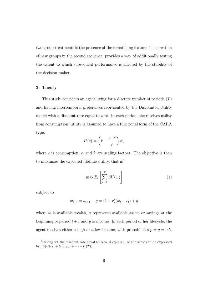
function establishes a recursive relation between current and future decisions.

In the specific case of this study, some restrictions have been imposed on

variables. In particular, as anticipated, borrowing is not allowed (wt ≥ 0)

and all variables are rounded to the nearest integer. For this reason a nu-

merical solution of the problem had to be computed. The figure below shows

an example of an optimal solution determined by the Maple optimization

program.

Figure 1 An example of optimal solution

4. Experimental Design

In order to investigate the difference between individual and group plan-

ning within the intertemporal consumption framework, an experiment com-

posed of three treatments has been designed.

8

In each session participants played two independent sequences of fifteen

periods each. The final payoff was calculated on the results of one sequence.

At the end of the experiment there was a public procedure devised to ran-

domly determine the paying sequence. Instructions provided definition for

sequences and periods and also clarified what was meant by “independence”

of sequences. In each period of a sequence, participants would receive income,

denominated in “tokens”, that, together with previous savings would deter-

mine available wealth5. Instructions asked participants to decide how many

of their available tokens they would like to convert into “points”, knowing

that, at the end of the experiment, the total points accumulated would be

converted into money at a fixed rate (two Euros per 100 points). Instructions

also explained how to use the utility function (called “conversion function”),

briefly pointing out some important features, such as the property of decreas-

ing marginal utility6.

The probability of receiving a high or low income was set to 0.5. This

probability was made public knowledge. In each period of a sequence, income

was determined by a random draw from an opaque bag and was the same for

all participants in a session. The two events were colour coded such that the

bag contained an equal number of balls in both colours. At the beginning

of the experiment, one participant was asked to publicly open the bag and

count the balls. When drawing a ball, participants were asked to shuffle the

5During the experiment expressions like “income”, “wealth”, “consumption” or “util-ity” were carefully avoided.

6Again, there was no explicit reference to decreasing marginal utility but to “incrementsat a decreasing rate”.

9

contents of the bag and then pick one ball to show to everyone. The ball

was then placed back into the bag so as not to alter the probability of future

draws.

When making a decision, participants were made aware that tokens saved

would produce interest (at a fixed rate of 0.2) which, in the next period, would

be summed to savings and income to give the total of tokens available for

conversion. Instructions also explained that all variables were integers. Par-

ticipants were advised that interest would be rounded to the nearest integer,

and examples were given to clarify this procedure. Finally, participants were

told at different points of instructions that any savings left over at the end

of the last period would be worthless.

4.1. Individual decision making

In the case of individual planning (IND), participants were randomly as-

signed to computers. Any contact with others, apart from the experimenters,

was forbidden. For each decision participants had one minute where they

could try different conversions (using a calculator), however they were not

permitted to confirm their decision before the end of the minute. This pro-

cedure was implemented to induce participants to think about their strategy.

The software included a calculator to allow participants to view the conse-

quences of their decisions (in terms of future interest, savings and utility)

and to compare alternative strategies.

10

4.2. Group decision making

We use two treatments for group decision making: group baseline (GR-

BSL) and group rematching (GR-R). Both treatments involve groups of two

members. In GR-BSL groups were composed of the same members in the first

and in the second sequence. In GR-R a random matching rule was enforced,

so that groups were formed at the beginning of each sequence and the same

participants could not be partners more than once. This was implemented in

an attempt to isolate the performance of groups to the greatest extent possi-

ble. As in the treatment with individuals, a strict no talking rule was imposed

(with the exception of members within the group). Groups had a total of

three minutes to discuss and confirm a decision; however, a choice could only

be confirmed after the first minute. In order to limit the length of sessions,

after the three minutes time, if no decision was confirmed by members, the

computer would randomly choose between the last two proposals7. To fa-

cilitate interactions between members and increase information about group

strategies, an instant messaging system was made available to chat within

the group. Participants were informed about the fact that the software was

recording all of their messages and that the chat system was available from

the beginning to the end of each period. Participants could freely exchange

messages with their partner but they were not allowed to reveal their identity,

encourage their partner to share identifying information or use inappropriate

7The software recorded all proposals. When members did not confirm a decision withinthree minutes, the computer would pick the last proposal of each member and then ran-domly choose one of those as representative of the group. This did not happen veryfrequently. We recorded 58 cases of “disagreement” out of 840 decisions (7%) in GR-Rand 23 cases out of 900 decisions in GR-BSL (2.5%). Preliminary regressions suggestedthat disagreement was not a significant regressor.

11

language8. Instructions provided a detailed explanation of how to interact

with one’s partner and how to confirm a decision. Partners had to take turns

in making proposals as well as take turns as “first proposers”, that is, who

initiated the exchanges of proposals in a period9. The person whose turn

it was to make a proposal, selected the available button labeled “Propose”

which submitted it to their partner. After sending a proposal the turn then

passed to the other group member, who had to make a counter-proposal.

During this process, both partners had a calculator available to try differ-

ent conversions and check the consequences of each of them. As mentioned

above, partners could not confirm a group decision before one minute. For

that reason, they could only use the “Propose” button; a “Confirm” button

was only available after the one minute time limit. To confirm a proposal, a

group member had to press the “Confirm” button; otherwise she could still

make a counter-proposal and pass the turn to her partner.

After instructions were provided in both individual and group planning

sessions, a quiz was distributed to test participants’ understanding of the

experiment. Participants were then given some time to practice with the

software, in particular with the calculator and the system for group interac-

tion. All sets of instructions included a graph of the utility function and two

tables with examples of conversions and of the interest mechanism10.

8After analyzing all messages exchanged, findings suggest that participants generallycomplied with these rules.

9In the first period of a sequence, the computer would randomly determine the “firstproposer”; after that, partners would take turns exchanging proposals.

10This material is available on request.

12

4.3. Payment

The final payoff was the conversion into money of the total of points

accumulated in one sequence. The computer randomly determined which se-

quence would be used for payment. Instructions explained that points would

be converted into money at a fixed rate of two Euros per 100 points. In

the group treatments, both partners would receive the payoff calculated as

described above. This design choice was made so as to not alter the framing

of incentives between treatments. Also, the choice of not imposing a sharing

rule or allowing participants to enter into bargaining on how to share the

payoff, was motivated by considerations on how this might have altered the

behaviour of participants during the experiment.

Experimental sessions were run at both the Universita degli Studi di

Salerno and LabSi at Universita degli Studi di Siena (four sessions for GR-R,

five for GR-BSL, three for IND). Participants were undergraduate students of

different disciplines. Overall, 28 participants took part in the sessions for in-

dividual decision making, 56 participants took part in the group sessions with

rematching (28 groups of two), and 60 participants took part in the group

baseline treatment (30 groups of two). The experiment was programmed and

conducted with the software z-Tree (Fischbacher, 2007).

5. Findings

A first approach in analyzing individual and group planning is to see

how much, on average, participants deviated from optimal utility. This is

13

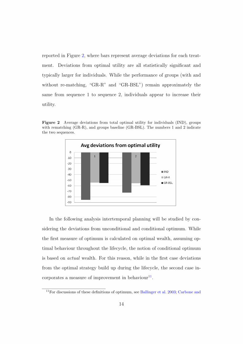
reported in Figure 2, where bars represent average deviations for each treat-

ment. Deviations from optimal utility are all statistically significant and

typically larger for individuals. While the performance of groups (with and

without re-matching, “GR-R” and “GR-BSL”) remain approximately the

same from sequence 1 to sequence 2, individuals appear to increase their

utility.

Figure 2 Average deviations from total optimal utility for individuals (IND), groupswith rematching (GR-R), and groups baseline (GR-BSL). The numbers 1 and 2 indicatethe two sequences.

In the following analysis intertemporal planning will be studied by con-

sidering the deviations from unconditional and conditional optimum. While

the first measure of optimum is calculated on optimal wealth, assuming op-

timal behaviour throughout the lifecycle, the notion of conditional optimum

is based on actual wealth. For this reason, while in the first case deviations

from the optimal strategy build up during the lifecycle, the second case in-

corporates a measure of improvement in behaviour11.

11For discussions of these definitions of optimum, see Ballinger et al. 2003; Carbone and

14

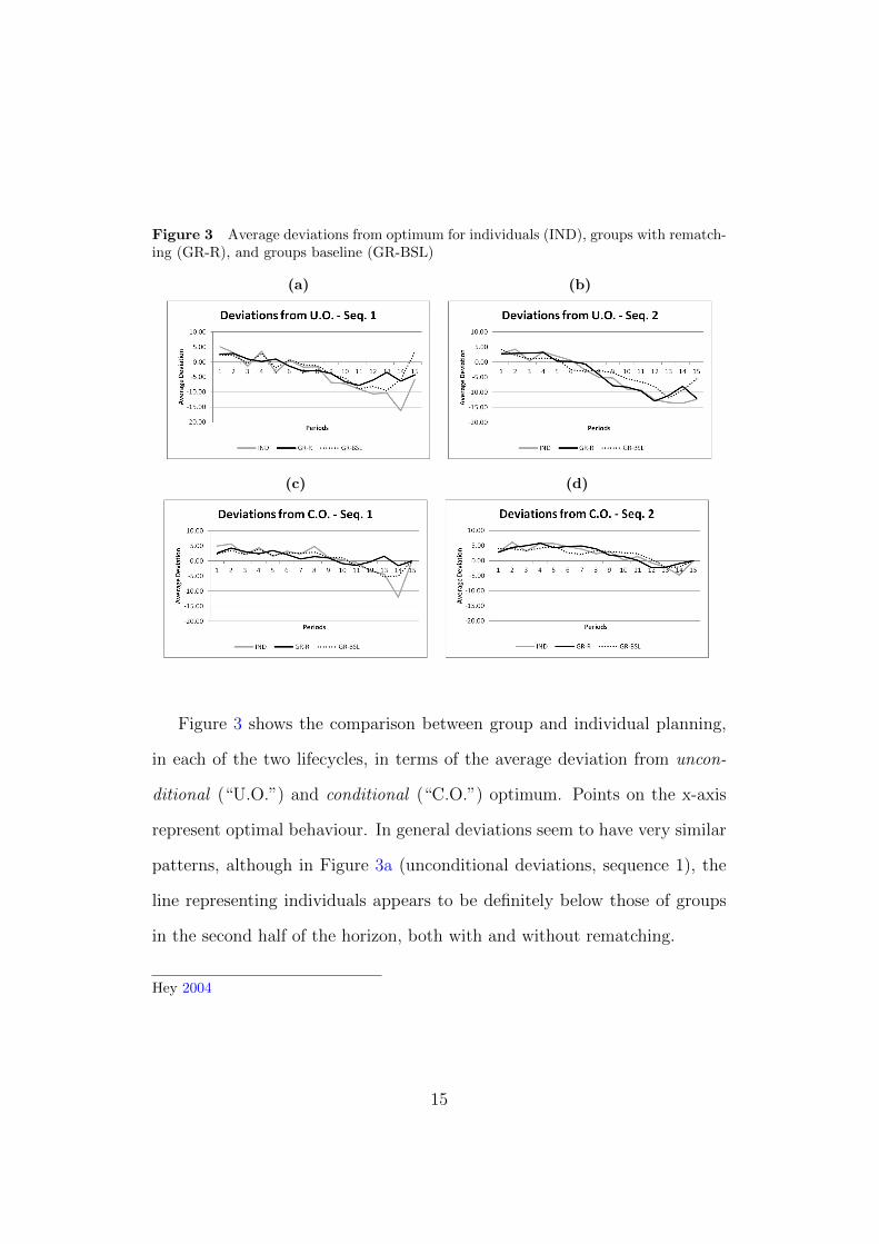
Figure 3 Average deviations from optimum for individuals (IND), groups with rematch-ing (GR-R), and groups baseline (GR-BSL)

(a) (b)

(c) (d)

Figure 3 shows the comparison between group and individual planning,

in each of the two lifecycles, in terms of the average deviation from uncon-

ditional (“U.O.”) and conditional (“C.O.”) optimum. Points on the x-axis

represent optimal behaviour. In general deviations seem to have very similar

patterns, although in Figure 3a (unconditional deviations, sequence 1), the

line representing individuals appears to be definitely below those of groups

in the second half of the horizon, both with and without rematching.

Hey 2004

15

5.1. Regression Analysis

In order to get a better understanding of how groups performed, com-

pared to individuals, we have run a first set of regressions to compare our

treatments (Table 1). We then proceeded to analyze each treatment in iso-

lation with the objective of detecting how individuals and groups performed

across sequences (Table 2). All estimations use the deviation from opti-

mum as the dependent variable, defined as the logarithm of the absolute

value of the deviation from optimum (both unconditional and conditional)12.

This way estimated coefficients are interpreted in terms of percentage of

variation, with positive (negative) signs representing increasing (decreasing)

deviations. Also, the observations of participants who did not consume all

of their wealth in the last period have been dropped13. All estimations dis-

cussed below include individual random effects and heteroskedasticity-robust

standard errors.

Table 1 offers an overview of the comparisons between the treatments of

our experiment. For each of them, two regressions are presented, one for

each of the two sequences played by participants14. In Table 1 the variable

we are most interested in is “Treatment”, a dummy variable used to identify

the treatment effect. These regressions all refer to deviations from uncondi-

tional optimum. In the case of conditional deviations, the crucial variable

12For a similar approach see Brown et al. (2009)13This is because instructions clearly stated that the best strategy in the last period was

to consume all the available wealth. Failure to do so is therefore interpreted as a mistake,rather than part of one’s strategy. This occurred six times in the case of individual decisionmaking, five times in the case of groups with rematching and only once in the case of groupswithout.

14The column “(1)” always corresponds to Sequence 1, and Column “(2)” to Sequence2.

16

Table 1 Comparison of treatments - Dev. from uncond. optimum

IND vs GR-R IND vs GR-BSL GR-R vs GR-BSL

(1) (2) (1) (2) (1) (2)

Treatment -0.267∗∗∗ 0.0289 -0.265∗ -0.163 -0.0445 0.251∗∗

(-4.11) (0.37) (-2.41) (-1.64) (-0.49) (2.81)

Period 0.109∗∗∗ 0.125∗∗∗ 0.115∗∗∗ 0.109∗∗∗ 0.110∗∗∗ 0.105∗∗∗

(17.20) (24.05) (18.88) (19.07) (17.57) (19.16)

Income -0.0121 0.00709 -0.0542 0.0283 0.000820 -0.00674(-0.22) (0.14) (-1.03) (0.53) (0.02) (-0.12)

Wealth 0.00185 0.000738 0.00304∗ -0.00306 0.00179 0.000554(1.46) (0.42) (2.51) (-1.86) (1.04) (0.25)

Male -0.0979 -0.244∗∗ -0.170 -0.101 -0.0825 -0.105(-1.45) (-3.21) (-1.58) (-1.07) (-0.67) (-0.88)

Mixed -0.182∗ -0.0875 -0.122 -0.111 -0.109 -0.0621(-2.03) (-0.88) (-0.87) (-0.84) (-0.95) (-0.57)

Constant 1.010∗∗∗ 0.861∗∗∗ 0.988∗∗∗ 0.982∗∗∗ 0.742∗∗∗ 0.756∗∗∗

(12.36) (11.10) (9.20) (10.84) (6.27) (6.63)

Observations 797 795 823 822 826 823R2 0.321 0.424 0.326 0.299 0.297 0.298

t statistics in parentheses∗ p < 0.05, ∗∗ p < 0.01, ∗∗∗ p < 0.001

IND vs GR-R. “Treatment”=1 is for GR-R

IND vs GR-BSL. “Treatment”=1 is for GR-BSL

GR-R vs GR-BSL. “Treatment”=1 is for GR-R

(1) and (2) indicate sequence 1 and sequence 2

17

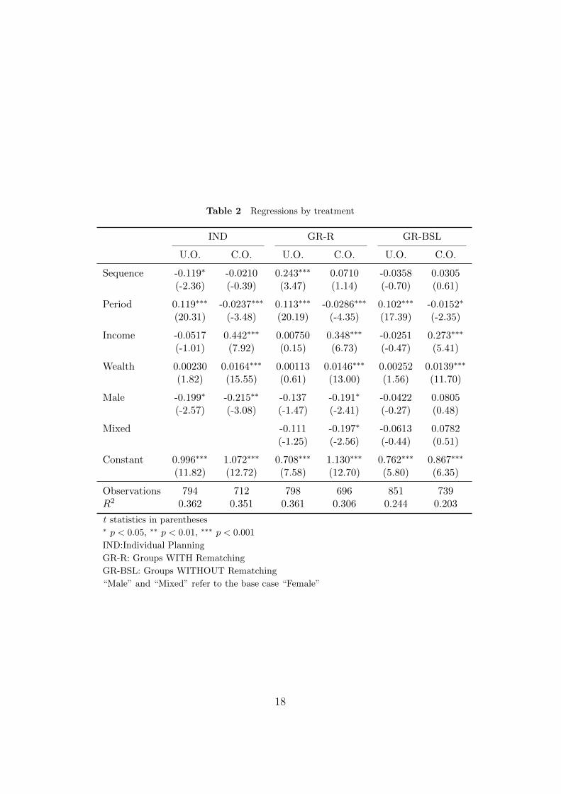
Table 2 Regressions by treatment

IND GR-R GR-BSL

U.O. C.O. U.O. C.O. U.O. C.O.

Sequence -0.119∗ -0.0210 0.243∗∗∗ 0.0710 -0.0358 0.0305(-2.36) (-0.39) (3.47) (1.14) (-0.70) (0.61)

Period 0.119∗∗∗ -0.0237∗∗∗ 0.113∗∗∗ -0.0286∗∗∗ 0.102∗∗∗ -0.0152∗

(20.31) (-3.48) (20.19) (-4.35) (17.39) (-2.35)

Income -0.0517 0.442∗∗∗ 0.00750 0.348∗∗∗ -0.0251 0.273∗∗∗

(-1.01) (7.92) (0.15) (6.73) (-0.47) (5.41)

Wealth 0.00230 0.0164∗∗∗ 0.00113 0.0146∗∗∗ 0.00252 0.0139∗∗∗

(1.82) (15.55) (0.61) (13.00) (1.56) (11.70)

Male -0.199∗ -0.215∗∗ -0.137 -0.191∗ -0.0422 0.0805(-2.57) (-3.08) (-1.47) (-2.41) (-0.27) (0.48)

Mixed -0.111 -0.197∗ -0.0613 0.0782(-1.25) (-2.56) (-0.44) (0.51)

Constant 0.996∗∗∗ 1.072∗∗∗ 0.708∗∗∗ 1.130∗∗∗ 0.762∗∗∗ 0.867∗∗∗

(11.82) (12.72) (7.58) (12.70) (5.80) (6.35)

Observations 794 712 798 696 851 739R2 0.362 0.351 0.361 0.306 0.244 0.203

t statistics in parentheses∗ p < 0.05, ∗∗ p < 0.01, ∗∗∗ p < 0.001

IND:Individual Planning

GR-R: Groups WITH Rematching

GR-BSL: Groups WITHOUT Rematching

“Male” and “Mixed” refer to the base case “Female”

18

“Treatment” was always not significant. These estimations are reported in

the Appendix (Table 5).

Finding 1. Individuals and groups (in both group treatments) do not dif-fer significantly in the way they improve their planning within a sequence(deviations from conditional optimum).

Regressions show that there is a clear difference in how they solve the in-

tertemporal problem (deviations from unconditional optimum). When com-

paring individuals and groups with rematching (column “IND vs GR-R”),

results suggest that while in the first sequence groups deviate significantly

less (about 27%) than individuals (column (1)), this difference seems to dis-

appear in the second lifecycle (column (2)). This result may suggest that

in the second lifecycle either individuals improved or that groups did worse.

Another possibility is that both of these statements are true. Regressions

in Table 2 help shed light on this conjecture. When looking at the effect

of playing the second sequence (the variable “Sequence”), results show that

while individuals were able to improve their planning (deviating about 12%

less in sequence 2, column “IND”), groups did significantly worse (about

24%, column “GR-R”). When looking at the performance of groups without

rematching, we find three interesting results. First, similarly to GR-R these

groups are better than individuals in sequence 1, but this difference becomes

not significant in sequence 2 (Table 1, column “IND vs GR-BSL”). Second,

when directly comparing the two types of group (Table 1, column “GR-R

vs GR-BSL”) results show that groups with rematching perform worse than

those without in sequence 2 (while in the first sequence the difference is

not significant). Finally, regressions in Table 2 show that the performance

19

of groups without rematching has not significantly changed across sequences.

Finding 2. Groups seem to do better than individuals when they first ap-proach the problem (in the first sequence).

Finding 3. Individuals improve their planning across sequences; the perfor-mance of groups without rematching is not significantly different, while groupswith rematching perform worse.

Finding 4. In the second sequence, the difference between the performanceof individuals and groups is not significant. Groups in the rematching treat-ment (GR-R) deviate more from optimum than groups without rematching(GR-BSL).

The fact that, in the second sequence, groups with rematching perform

worse than individuals and groups without rematching, may have two pos-

sible explanations. On the one hand the rematching mechanism itself may

have a detrimental effect on planning. On the other hand, differences in

the actual distribution of income may have driven differences in performance

across treatments, and across sequences. Table 2 shows that, in all treat-

ments, wealth (“Wealth”) and a high income (“Income”) cause a significant

increase in the deviation from optimum. In principle, this implies that the

decline in performance of groups with rematching in sequence 2 may also be

explained by a more favourable realization of the income distribution (i.e.

they were luckier than participants in other treatments). A simple way to

test this hypothesis is to compare all treatments with respect to the average

total income earned in each sequence and the number of “bad” draws. As

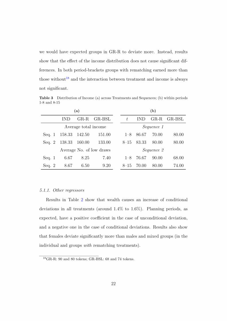
Table 3a shows, groups with rematching were indeed luckier in sequence 2,

compared to participants in other treatments and to sequence 1. They moved

20

from the lowest average income to the highest. Although this may help to ex-

plain why the performance of these groups is worse in the second sequence,

this analysis alone does not clarify to what extent this result is driven by

the effect of rematching and/or of income. In an attempt to further clarify

this point, we have looked at the actual distributions of income within the

first and last eight periods of each sequence (See Table 3b). We have also

run regressions relative to these period-brackets. The models that have been

estimated include an additional variable, the interaction between treatment

and income, used to detect differences between treatments when earning a

high income15. The following discussion is focussed on the analysis relevant

to the Findings 3 and 4. Results show that learning across sequences is sta-

tistically significant for all treatments, but only with respect to the 8-to-15

period-bracket16. While the performances of individuals and groups without

rematching improve across sequences17, groups with rematching seem to do

significantly worse. The effect of receiving a high income is always found to

be not significant, in the two period-brackets of the second sequence, when

comparing GR-R and IND. However, in those subsets of periods groups with

rematching always earned more than individuals, receiving an above-average

(90 tokens, periods 1 to 8) or exactly average (80 tokens periods 8 to 15)

income, compared to individuals (76.67 and 70 tokens, respectively). If dif-

ferences between treatments were caused by the actual distribution of income

15The following discussion refers to the deviation from unconditional optimum, as ourmain findings. These regressions are available on request from the authors.

16These regressions replicate those reported in Table 2, with the exception that they arerestricted to periods 1 to 8 or 8 to 15.

17In GR-BSL the effect of the second sequence is only significant at 5%.

21

we would have expected groups in GR-R to deviate more. Instead, results

show that the effect of the income distribution does not cause significant dif-

ferences. In both period-brackets groups with rematching earned more than

those without18 and the interaction between treatment and income is always

not significant.

Table 3 Distribution of Income (a) across Treatments and Sequences; (b) within periods1-8 and 8-15

(a)

IND GR-R GR-BSL

Average total income

Seq. 1 158.33 142.50 151.00

Seq. 2 138.33 160.00 133.00

Average No. of low draws

Seq. 1 6.67 8.25 7.40

Seq. 2 8.67 6.50 9.20

(b)

t IND GR-R GR-BSL

Sequence 1

1–8 86.67 70.00 80.00

8–15 83.33 80.00 80.00

Sequence 2

1–8 76.67 90.00 68.00

8–15 70.00 80.00 74.00

5.1.1. Other regressors

Results in Table 2 show that wealth causes an increase of conditional

deviations in all treatments (around 1.4% to 1.6%). Planning periods, as

expected, have a positive coefficient in the case of unconditional deviation,

and a negative one in the case of conditional deviations. Results also show

that females deviate significantly more than males and mixed groups (in the

individual and groups with rematching treatments).

18GR-R: 90 and 80 tokens; GR-BSL: 68 and 74 tokens.

22

5.2. Chat messages and heuristics

In order to gather more information on the relation between group plan-

ning and the deviation from optimum, a number of heuristics were extrap-

olated from the chat messages, representing the strategies discussed by par-

ticipants during the experiment19. Given the nature of the task, the mes-

sages exchanged within each group in a sequence are a mix of proposals,

counter-proposals, various planning considerations and comments that are

not relevant for the problem. For this reason, any attempt to categorize each

message within a heuristic is very difficult. Nevertheless, following Carbone

(2005) we have summarized the strategies emerging from chat messages ac-

cording to the following heuristics: (1) consume a fraction of savings (2) keep

consumption constant (3) consume a fraction of wealth (C/W) (4) consume

a fraction of income (C/Y) (5) consume all income in each period (6) con-

sume all wealth in each period (7) unconditional optimum (8) conditional

optimum. These heuristics can be rewritten as follows:

1. Ct = β1 ∗ st + ε1

2. Ct = β2 ∗ ct−1 + ε2

3. Ct = β3 ∗ C/W + ε3

4. Ct = β4 ∗ C/Y + ε4

For each group and individual we have estimated the parameters, βi and

εi, associated with the above heuristics20, using their actual consumption

19We thankfully acknowledge the comments of the editor and two referees, which havehelped sharpen the focus of this analysis.

20The heuristics from 5 to 8 do not need any parameter to be estimated.

23

choices. For each strategy we were then able to determine the fitted values

of consumption21 and compute their deviations from actual choices. This

way, groups and individuals were attributed the heuristic for which the sum

of squared deviations was minimized. Results are summarized in Table 4.

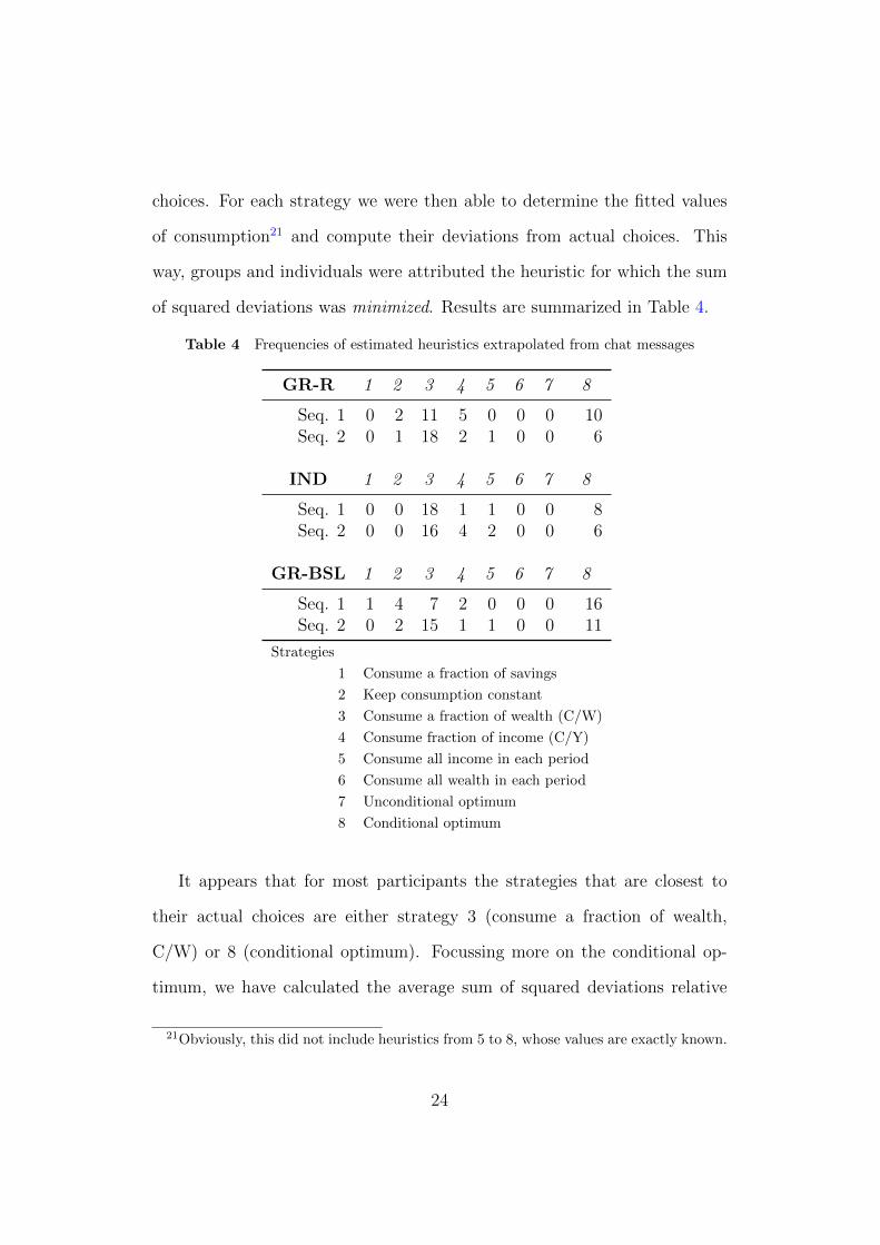
Table 4 Frequencies of estimated heuristics extrapolated from chat messages

GR-R 1 2 3 4 5 6 7 8

Seq. 1 0 2 11 5 0 0 0 10Seq. 2 0 1 18 2 1 0 0 6

IND 1 2 3 4 5 6 7 8

Seq. 1 0 0 18 1 1 0 0 8Seq. 2 0 0 16 4 2 0 0 6

GR-BSL 1 2 3 4 5 6 7 8

Seq. 1 1 4 7 2 0 0 0 16Seq. 2 0 2 15 1 1 0 0 11

Strategies

1 Consume a fraction of savings

2 Keep consumption constant

3 Consume a fraction of wealth (C/W)

4 Consume fraction of income (C/Y)

5 Consume all income in each period

6 Consume all wealth in each period

7 Unconditional optimum

8 Conditional optimum

It appears that for most participants the strategies that are closest to

their actual choices are either strategy 3 (consume a fraction of wealth,

C/W) or 8 (conditional optimum). Focussing more on the conditional op-

timum, we have calculated the average sum of squared deviations relative

21Obviously, this did not include heuristics from 5 to 8, whose values are exactly known.

24

to this strategy only. Results show that in sequence 1, not only do groups

use it more frequently than individuals, but they do it with a significantly

smaller degree of error (Average Sum of Squared Deviations: IND=2564.87;

GR-R=1279.3; GR-BSL=749.56). In the second sequence, although the fre-

quency of strategy 8 decreases in all treatments, individuals seem to use

it more effectively, with a dramatic reduction of the average of the sum of

squared deviations (Average Sum of Squared Deviations: IND=361.5; GR-

R=3137.5; GR-BSL=477.45). On the other hand, groups with rematching

on average do significantly worse than in sequence 1 and with respect to

individuals and group without rematching.

6. Discussion

We have presented the results of an experiment comparing individual and

group decision making in an intertemporal consumption/saving problem. In

the experiment we have used two different types of groups, with (GR-R) and

without (GR-BSL) rematching of their members across the two sequences

they play. The main finding is that groups and individuals are indeed dif-

ferent in how they solve the lifecycle problem. When first approaching the

problem, groups seem to be clearly better than individuals. However, by the

second sequence this advantage disappears as individuals display a signifi-

cant learning effect, which does not occur in group planning. In the GR-BSL

treatment their performance remains approximately the same. However, in

the GR-R treatment we observe a significant decline in group performance.

The finding that the performance of groups with rematching declines

25

between sequences seems to be confirmed by the analysis of the estimated

planning heuristics, which shows that in the GR-R treatment, groups tend

to use the conditional optimum strategy with a higher degree of error (com-

pared to the first sequence). In order to shed more light on this finding, we

have also looked at the potential effects of the actual realizations of income

across treatments, sequences, and subsets of periods of each sequence. Re-

sults suggest that although groups in the GR-R treatment earned more in the

second sequence (compared to other treatments and to the first sequence),

this does not seem to have caused the difference in performance we observed

across treatments.

While the results of the individual treatment are in line with existing

literature, the question remains, what happened in the second sequence of

group treatments? Why are groups unable to improve their planning? In

the case of GR-R, as discussed above, the answer seems to be connected to

the role of rematching. However, the GR-BSL case is quite different. This

treatment is most similar to the individual treatment, the critical difference

being the nature of the agents. A review of chat messages reveals that groups

tend to be inconsistent in how they follow a plan during a sequence. This

seems to be related mainly to the process by which group members slowly

try to find an agreement on group planning. It takes some time for them to

agree on a strategy or find some understanding about how to solve the prob-

lem. Although we do not have specific information regarding the individual

decision-making process, we conjecture this might be a key contributing fac-

tor in the difference in performance observed between groups and individuals.

26

While groups have an immediate advantage, individuals seem to be better

equipped to reap the benefits of learning and experience.

7. References

Baker, R. J., Laury, S. K., and Williams, A. W. (2008). Comparing small-

group and individual behavior in lottery-choice experiments. Southern

Economic Journal, 75(2):367–382.

Ballinger, T. P., Palumbo, M. G., and Wilcox, N. T. (2003). Precaution-

ary saving and social learning across generations: an experiment. The

Economic Journal, 113(490):920–947.

Bateman, I. J. and Munro, A. (2005). An experiment on risky choice amongst

households. The Economic Journal, 115(502):C176–C189.

Bone, J., Hey, J. D., and Suckling, J. (1999). Are groups more (or less)

consistent than individuals? Journal of Risk and Uncertainty, 18(1):63–

81.

Bornstein, G. and Yaniv, I. (1998). Individual and group behavior in the

ultimatum game : Are groups more rational players ? Experimental

Economics, 108(1):101–108.

Brown, A. L., Chua, Z. E., and Camerer, C. F. (2009). Learning and vis-

ceral temptation in dynamic saving experiments. Quarterly Journal of

Economics, 124(1):197–231.

Browning, M. and Lusardi, A. (1996). Household saving: Micro theories and

micro facts. Journal of Economic Literature, 34(4):1797–1855.

27

Carbone, E. (2005). Demographics and behaviour. Experimental Economics,

8:217–232.

Carbone, E. and Duffy, J. (2014). Lifecycle consumption plans, social learn-

ing, and external habit: Experimental evidence. Journal of Economic

Behavior and Organization, 106:413–427.

Carbone, E. and Hey, J. D. (2004). The effect of unemployment on consump-

tion: an experimental analysis. The Economic Journal, 114(497):660–683.

Charness, G. and Jackson, M. O. (2007). Group play in games and the role

of consent in network formation. Journal of Economic Theory, 136(1):417–

445.

Charness, G. and Sutter, M. (2012). Groups make better self-interested

decisions. Journal of Economic Perspectives, 26(3):157–176.

Cooper, D. J. and Kagel, J. H. (2005). Are two heads better than one? team

versus individual play in signaling games. American Economic Review,

95(3):477–509.

Denant-Boemont, L., Diecidue, E., and l’Haridon, O. (2013). Patience

and time consistency in collective decisions. INSEAD Working Paper.

2013/109/DSC.

Feri, F., Irlenbusch, B., and Sutter, M. (2010). Efficiency gains from team-

based coordinationlarge-scale experimental evidence. The American Eco-

nomic Review, 100(4):1892–1912.

28

Fischbacher, U. (2007). z-tree: Zurich toolbox for ready-made economic

experiments. Experimental Economics, 10(2):171–178.

Gillet, J., Schram, A., and Sonnemans, J. (2009). The tragedy of the com-

mons revisited: The importance of group decision-making. Journal of

Public Economics, 93(56):785–797.

Kocher, M. G. and Sutter, M. (2005). The decision maker matters: Indi-

vidual versus group behaviour in experimental beauty-contest games. The

Economic Journal, 115:200–223.

Maciejovsky, B., Sutter, M., Budescu, D. V., and Bernau, P. (2010). Teams

make you smarter: Learning and knowledge transfer in auctions and mar-

kets by teams and individuals. IZA Discussion Paper no. 5105.

Masclet, D., Loheac, Y., Denant-Boemont, L., and Colombier, N. (2009).

Group and individual risk preferences : a lottery-choice experiment with

self-employed and salaried workers. Journal of Economic Behavior and

Organization, 70(3):470–484.

Shupp, R. and Williams, A. R. (2008). Risk preference differentials of small

groups and individuals. The Economic Journal, 118(525):258–283.

Sutter, M., Czermak, S., and Feri, F. (2010). Strategic sophistication of

individuals and teams in experimental normal-form games. IZA Discussion

Paper no. 4732.

Zhang, J. and Casari, M. (2012). How groups reach agreement in risky

choices: an experiment. Economic Enquiry, 50(2):502–515.

29

Appendices

A. Instructions - NOT FOR PUBLICATION

This Appendix contains the instructions of the individual (IND) and

group with rematching (GR-R) treatments. The instructions of the group

treatment without rematching (GR-BSL) are the same as the GR-R case,

except for the part related to rematching.

A.1. Individual Decision Making

Welcome!

This is an experiment on decision making. The experiment will last about

1 hour and a half. Please read these instructions carefully as you have the

chance to earn money depending on your decisions. If you have any questions

please raise your hand. The experimenter will answer in private. You are

not allowed to talk to other participants in the experiment.

The experiment consists of 2 independent “sequences”, each one composed of

15 periods. Sequences are independent because there is no relation between

them. This means that your choices in one sequence will not influence future

sequences. However, please note that, within one sequence, your decision in

each period will influence subsequent periods (for example, your decision in

period 1 will have consequences for period 2 and so on).

At the beginning of each period you will receive an amount of tokens that will

30

be available to you. You have to decide how many tokens you want to convert

into points. You can convert a number of tokens between 0 and the amount

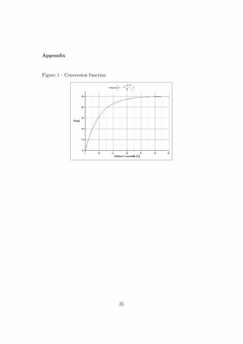
available to you. The conversion function of tokens to points is reported in

Figure 1 (Appendix). This figure shows graphically the conversion of tokens

to points in a continuous interval. You may also look at Table 1 (Appendix)

where some examples of conversions are provided. Please note that that the

number of points obtained from the conversion increases as the number of

tokens converted increases; however, increments are realized at a decreasing

rate, that is, the difference in points obtained by converting 6 tokens rather

than 5 is bigger than the difference between converting 16 tokens rather than

15. Finally, please note that the more tokens are converted in each period,

the less tokens are saved for conversion in future periods. Please note that,

before period 15 (the last period) is reached, tokens not converted will be

saved for the next period. Savings will earn interest, thus increasing the

amount of tokens available in the following period. When period 15 (the last

period) is reached, any tokens left (that is, not converted) will be worthless.

Your payoff, at the end of the experiment, will be calculated on the deci-

sions you have made in ONE of the above mentioned “sequences”. This

sequence will be randomly selected among the 2 played. This means that

your payment will be calculated based on the decisions you made during the

15 periods composing the randomly selected sequence. In particular, your

payment will be the conversion in Euros of the total amount of points earned

in the selected sequence, using a conversion rate of 2 Euros each 100 points.

31

Periods and Decision Making

At the beginning of each period, you will be randomly assigned a number of

tokens. This number may be “high” (15 tokens) or “low” (5 tokens). You

have 50% chance of receiving one of the two. It is important to note that

the amount of tokens received in one period does not affect the chances of

getting the same or the other amount in any following period.

From period 1 to period 14, if you have any tokens saved, they will earn

interest, at the rate of 20% (r = 0.2). Savings plus interest accumulated

will increase the number of tokens available to you in the following period.

Please remember that tokens not converted at the end of period 15 will be

worthless. Table 2 (Appendix) is available to you, reporting some examples

of calculation of interest.

At the beginning of each period you will be showed on the computer screen

the total of tokens available, consisting in:

1. Tokens earned in the period: 15 or 5

2. Tokens saved in the previous period (S)

3. Interest earned on savings: S x 0.2 (not rounded)

4. Tokens available for conversion rounded to the nearest integer (for ex-

ample, 3.4=3; 3.5=4 or 3.6=4): Tokens earned in the period (1.) +

Tokens saved in the previous period (2) + Interest earned on savings

32

(3.)

5. Total of points earned: sum of the points earned starting from period

1

Of course, in period 1 there will be no savings and no interest received, so

the number of tokens available to you will be equal to 15 or 5 tokens.

Within this screen you will be asked to enter the number of tokens you wish

to convert into points. You may change your decision in any moment before

pressing the “confirm” button. When this button is pressed your decision

will become irrevocable. You cannot move to the next decision before one

minute from the beginning of the current period. To make your decision you

may use a calculator to observe the consequences of your choice. Depend-

ing on the number entered, it is possible to see the related savings, interest

earned on savings in the next period and the number of points earned from

conversion. The use of the calculator will not make your choice final.

Once the first 15-period sequence has been completed, the following sequence

will start. As explained above, the experiment involves making decisions

through 2 sequences.

At the end of each sequence a summary of the choices made during the 15

periods will be provided.

Earnings

33

When the 2 sequences have been completed, your payment will be deter-

mined. One sequence will be randomly selected and you will receive the

conversion in Euros of the total amount to points earned in the selected se-

quence.

If you have any questions, please raise your hand and an experimenter will

be happy to assist you.

Right after these instructions a short quiz testing your comprehension of the

experiment will take place followed by 3 minutes practice with the conversion

function.

34

Appendix

Figure 1 - Conversion function

35

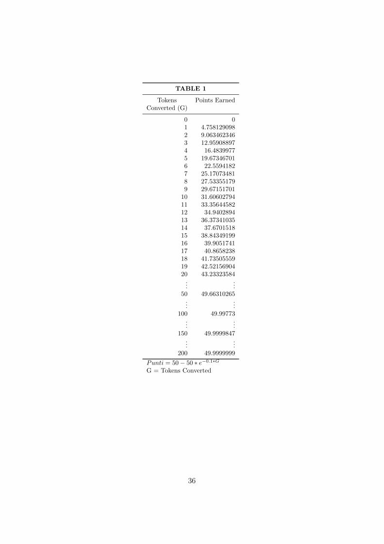
TABLE 1

Tokens Points EarnedConverted (G)

0 01 4.7581290982 9.0634623463 12.959088974 16.48399775 19.673467016 22.55941827 25.170734818 27.533551799 29.67151701

10 31.6060279411 33.3564458212 34.940289413 36.3734103514 37.670151815 38.8434919916 39.905174117 40.865823818 41.7350555919 42.5215690420 43.23323584

......

50 49.66310265...

...100 49.99773

......

150 49.9999847...

...200 49.9999999

Punti = 50 − 50 ∗ e−0.1∗G

G = Tokens Converted

36

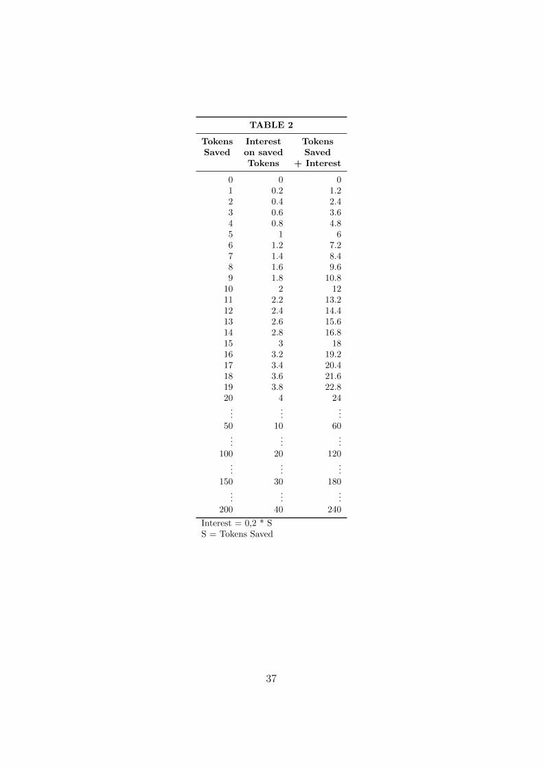
TABLE 2

Tokens Interest TokensSaved on saved Saved

Tokens + Interest

0 0 01 0.2 1.22 0.4 2.43 0.6 3.64 0.8 4.85 1 66 1.2 7.27 1.4 8.48 1.6 9.69 1.8 10.8

10 2 1211 2.2 13.212 2.4 14.413 2.6 15.614 2.8 16.815 3 1816 3.2 19.217 3.4 20.418 3.6 21.619 3.8 22.820 4 24

......

...50 10 60

......

...100 20 120

......

...150 30 180

......

...200 40 240

Interest = 0,2 * SS = Tokens Saved

37

A.2. Group Decision Making22

Welcome!

This is an experiment on decision making. You will be making decisions

in cooperation with another participant whose identity will be unknown to

you. The experiment will last about 1 hour and a half. Please read these

instructions carefully as you have the chance to earn money depending on

your decisions. If you have any questions please raise your hand. The ex-

perimenter will answer in private. You are not allowed to talk to other

participants in the experiment.

The experiment consists of 2 independent “sequences”, each one composed of

15 periods. Sequences are independent because there is no relation between

them. This means that your choices in one sequence will not influence future

sequences. However, please note that, within one sequence, your decision in

each period will influence subsequent periods (for example, your decision in

period 1 will have consequences for period 2 and so on).

During this experiment you will be part of a group composed of two indi-

viduals. The section “Groups and Decisions” explains how groups will be

formed, how to interact within a group and reach a decision.

At the beginning of each period your group will receive an amount of tokens

22The material referred to in the “Appendix” is the same for all sets of instructions andcan be consulted in subsection 1 (Individual Decision Making).

38

that will be available to you. You have to decide how many tokens you want

to convert into points. You can convert a number of tokens between 0 and

the amount available to you. The conversion function of tokens to points is

reported in Figure 1 (Appendix). This figure shows graphically the conver-

sion of tokens to points in a continuous interval. You may also look at Table

1 (Appendix) where some examples of conversions are provided. Please note

that that the number of points obtained from the conversion increases as the

number of tokens converted increases; however, increments are realized at a

decreasing rate, that is, the difference in points obtained by converting 6 to-

kens rather than 5 is bigger than the difference between converting 16 tokens

rather than 15. Finally, please note that the more tokens are converted in

each period, the less tokens are saved for conversion in future periods. Please

note that, before period 15 (the last period) is reached, tokens not converted

will be saved for the next period. Savings will earn interest, thus increasing

the amount of tokens available in the following period. When period 15 (the

last period) is reached, any tokens left (that is, not converted) will be worth-

less.

Your payoff, at the end of the experiment, will be calculated on the deci-

sions you have made in ONE of the above mentioned “sequences”. This

sequence will be randomly selected among the 2 played. This means that

your payment will be calculated based on the decisions you made during the

15 periods composing the randomly selected sequence. In particular, your

payment will be the conversion in Euros of the total amount of points earned

in the selected sequence, using a conversion rate of 2 Euros each 100 points.

39

Each member of the group will receive this payoff.

Periods

At the beginning of each period, you will be randomly assigned a number of

tokens. This number may be “high” (15 tokens) or “low” (5 tokens). You

have 50% chance of receiving one of the two. It is important to note that

the amount of tokens received in one period does not affect the chances of

getting the same or the other amount in any following period.

From period 1 to period 14, if you have any tokens saved, they will earn

interest, at the rate of 20% (r = 0.2). Savings plus interest accumulated will

increase the number of tokens available to the group in the following period.

Please remember that tokens not converted at the end of period 15 will be

worthless. Table 2 (Appendix) is available to you, reporting some examples

of calculation of interest.

Groups and Decisions

During each sequence you will be paired with another participant but you

will not know his/her identity. This matching will be random. At the end of

the first sequence, of 15 periods, new groups will be composed for the second

sequence, using again random matching.

40

Participants matched with you in a group will never have the opportunity to

know your identity. During the experiment is absolutely forbidden to reveal

your identity to the other group member (or try to know the identity of other

participants).

At the beginning of each period you will be showed on the computer screen

the total of tokens available, consisting in:

1. Tokens earned in the period: 15 or 5

2. Tokens saved in the previous period (S)

3. Interest earned on savings: S x 0.2 (not rounded)

4. Tokens available for conversion rounded to the nearest integer (for ex-

ample, 3.4=3; 3.5=4 or 3.6=4): Tokens earned in the period (1.) +

Tokens saved in the previous period (2) + Interest earned on savings

(3.)

5. Total of points earned: sum of the points earned starting from period

1

Of course, in period 1 there will be no savings and no interest received, so

the number of tokens available to you will be equal to 15 or 5 tokens.

In the same screen described above you will be asked to interact with the

other member of your group in order to make a decision. To do this the

following procedure will be employed:

41

1. You will have to take turns interacting with the other member

2. In the first period, one of the members of the group will be randomly

selected to start the interaction. In the periods following the first,

members will take turns initiating the interaction.

3. By pressing the button “PROPOSE”, the member of the group who

begins the interaction will send his/her proposal to the other member

and conclude his/her turn. After this, he/she will have to wait the other

member of the group to send his/her decision (accept the proposal or

make a new one)

4. It will not be possible to make a group decision before 1 minute. How-

ever, during this time group members will be able to exchange proposals

of conversion. At the end of the 1 minute time limit, each member of

the group, during his/her turn, will also have the opportunity to con-

firm the proposal received, hence turning it into the group decision,

which is irrevocable. The period is concluded when one of the group

members confirms a proposal. Hence, the approval of the other member

is not required.

5. Members will be able to keep interacting up to a time limit of 3 minutes.

After this limit, if a group decision has not been made, the computer

will randomly select one of the two members making his/her proposal

the final decision of the group.

6. When the minimum time to make a group decision is over (1 minute),

if the member whose turn it is to start interacting has not sent any

42

proposal to his partner, the turn will automatically pass to the other

member of the group.

Rules of Group Interaction

1. A group decision cannot be made before 1 minute since the start of

the current period. This means that even if an agreement is reached,

this decision cannot be confirmed before the minimum time limit of 1

minute is over.

2. On the screen used for group interaction, a calculator will be available

to you to verify the consequences of your choice. Depending on the

number of tokens entered, it is possible to see the related savings, in-

terest earned on savings in the next period and the number of points

earned from conversion.

3. A table, denominated “Group decision: current proposals” will be

shown on screen. This table is composed of two rows containing the

conversion proposals of each member of the group together with the re-

lated consequences. Your row is indicated by blue coloured characters.

4. Below this table a box will be available to enter your proposal of con-

version, which may be confirmed by pressing the button “PROPOSE”.

5. After 1 minute, that is, the minimum time allowed to make a group

decision, at each turn a button labeled “CONFIRM” will be available.

By pressing this button the group decision will be recorded (becoming

irrevocable)

43

6. An instant messaging (IM) system will also be available and operative

from the beginning to the end of the period. To use the chat simply

write your message and press enter on the keyboard. This way, your

message will be sent to your partner. Each message will be recorded.

While using the chat system it is absolutely forbidden to:

(a) Communicate one’s identity in any way (name, student number,

nicknames, etc.)

(b) Ask other participants questions that could lead to the disclosure

of identifying information

(c) Use inappropriate language (insults, etc.)

The experimenter will make sure that all the rules of chat usage are

respected. A violation of one of these rules will cause the cancellation

of the final payoff of the participant who committed the violation.

When the group decision has been made, the current period ends and a new

period begins.

Once the first 15-period sequence has been completed, the following sequence

will start. As explained above, the experiment involves making decisions

through 2 sequences.

At the end of each sequence a summary of the choices made during the 15

periods will be provided.

44

Earnings

When the 2 sequences have been completed, your payment will be deter-

mined. One sequence will be randomly selected and you will receive the

conversion in Euros of the total amount to points earned in the selected se-

quence.

If you have any questions, please raise your hand and an experimenter will

be happy to assist you.

Right after these instructions a short quiz testing your comprehension of the

experiment will take place followed by 3 minutes practice with the conversion

function and 3 minutes practice with the group-interaction system.

45

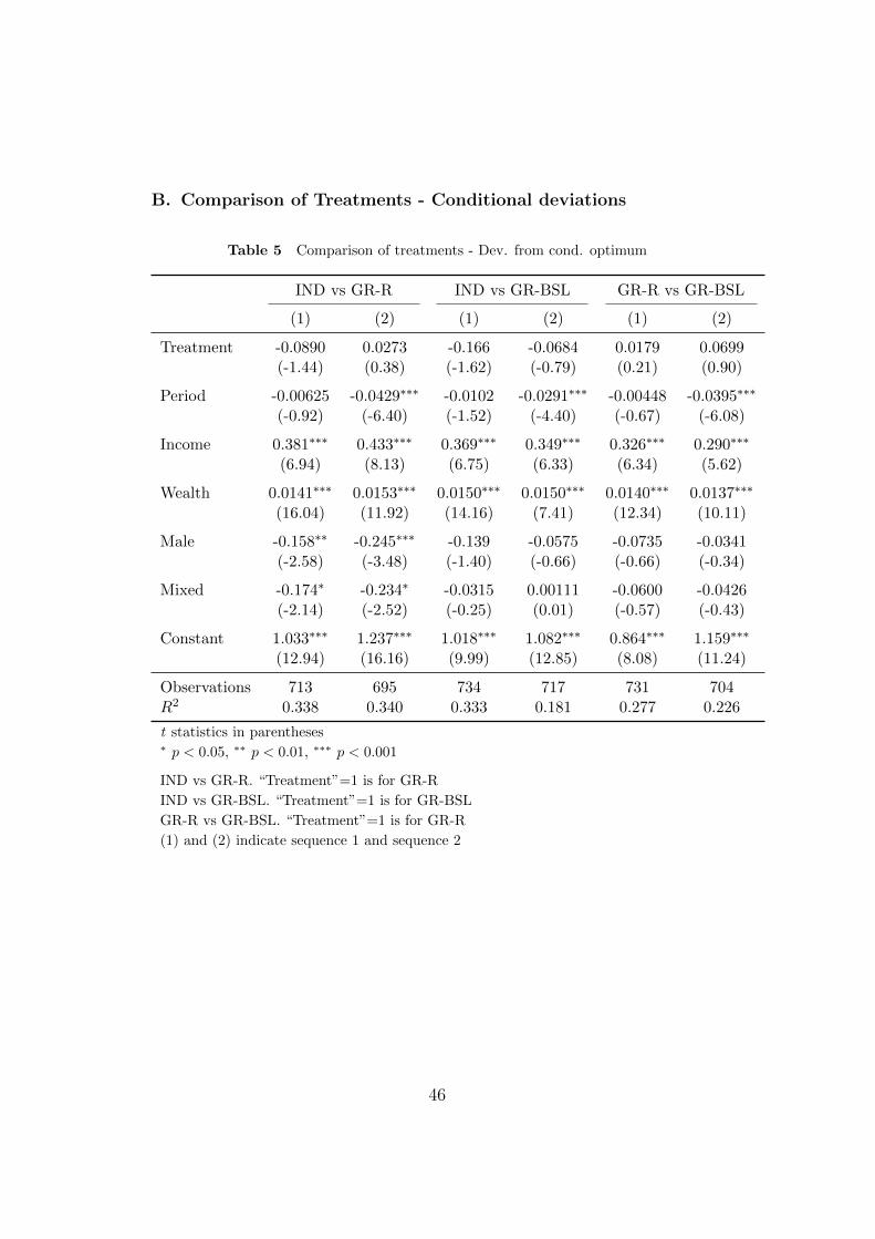
B. Comparison of Treatments - Conditional deviations

Table 5 Comparison of treatments - Dev. from cond. optimum

IND vs GR-R IND vs GR-BSL GR-R vs GR-BSL

(1) (2) (1) (2) (1) (2)

Treatment -0.0890 0.0273 -0.166 -0.0684 0.0179 0.0699(-1.44) (0.38) (-1.62) (-0.79) (0.21) (0.90)

Period -0.00625 -0.0429∗∗∗ -0.0102 -0.0291∗∗∗ -0.00448 -0.0395∗∗∗

(-0.92) (-6.40) (-1.52) (-4.40) (-0.67) (-6.08)

Income 0.381∗∗∗ 0.433∗∗∗ 0.369∗∗∗ 0.349∗∗∗ 0.326∗∗∗ 0.290∗∗∗

(6.94) (8.13) (6.75) (6.33) (6.34) (5.62)

Wealth 0.0141∗∗∗ 0.0153∗∗∗ 0.0150∗∗∗ 0.0150∗∗∗ 0.0140∗∗∗ 0.0137∗∗∗

(16.04) (11.92) (14.16) (7.41) (12.34) (10.11)

Male -0.158∗∗ -0.245∗∗∗ -0.139 -0.0575 -0.0735 -0.0341(-2.58) (-3.48) (-1.40) (-0.66) (-0.66) (-0.34)

Mixed -0.174∗ -0.234∗ -0.0315 0.00111 -0.0600 -0.0426(-2.14) (-2.52) (-0.25) (0.01) (-0.57) (-0.43)

Constant 1.033∗∗∗ 1.237∗∗∗ 1.018∗∗∗ 1.082∗∗∗ 0.864∗∗∗ 1.159∗∗∗

(12.94) (16.16) (9.99) (12.85) (8.08) (11.24)

Observations 713 695 734 717 731 704R2 0.338 0.340 0.333 0.181 0.277 0.226

t statistics in parentheses∗ p < 0.05, ∗∗ p < 0.01, ∗∗∗ p < 0.001

IND vs GR-R. “Treatment”=1 is for GR-R

IND vs GR-BSL. “Treatment”=1 is for GR-BSL

GR-R vs GR-BSL. “Treatment”=1 is for GR-R

(1) and (2) indicate sequence 1 and sequence 2

46