THE PRICING OF GREEN BONDS:ARE FINANCIAL INSTITUTIONS SPECIAL?

Serena Fatica Roberto Panzica Michela Rancan

Working paper no. 157

October 2019

1

The pricing of green bonds:

are financial institutions special?°

Serena Fatica Roberto Panzica Michela Rancan

This version: October 2019

Abstract

The financial system plays a major role in the transition to a low-carbon economy. We investigate this issue analyzing the recent developments and challenges in the bond and debt markets. First, we study the pricing of green bonds at issuance. We find a premium when green bonds are issued by supranational institutions and corporates while there is no effect for financial institutions. We also document an effect for external review and repeated access to this market. Second, we investigate lending decisions by banks issuing green bonds. Our results show that these lenders reduce their funding towards more polluting segments of the economy but limited to the amount of loans they granted as lead bank in the deal. This evidence may explain why we do not find a green premium for financial issuers. Yet it also suggests that the banking system may play a much larger role in channelling funds towards low-carbon activities, and thus reducing the environmental risks also for the financial system.

JEL Classification: G12, G20, Q52, Q53, Q54

° All authors are affiliated with the European Commission – Joint Research Centre, Directorate for Innovation and Growth, Economy and Finance Unit. Address: Via E. Fermi, Ispra (Italy). Comments from participants to the EC Academic Conference on Promoting Sustainable Finance, CBI Annual Meeting 2019, CREDIT 2019 in Venice, IFABS 2019 in Angers, the 13th Seminar on Financial Stability at the Bank of Romania are gratefully acknowledged. The opinions and views expressed in this paper are those of the authors only and should not be considered as official positions of the European Commission. Serena.Fatica@ec.europa.eu; Roberto.Panzica@ec.europa.eu; Michela.Rancan@ec.europa.eu.

2

Introduction The traditional public intervention to correct externalities, notably, in the form of taxes, subsidies and regulation, seems largely insufficient to address the current environmental and climate-related challenges. The sheer magnitude of these problems requires mobilizing a considerable amount of funds. In this area, finance has undoubtedly a key role to play. Among the activities and instruments of sustainable finance, green bonds represent one of the most promising market-based solutions to channel funds to environmentally beneficial projects, as well as to raise awareness of environmental risks. As a relatively new practice in corporate finance, there is no commonly agreed definition for green bonds. Speaking loosely, these fixed income securities differ from conventional debt instruments only in that they finance environmental or climate-related projects. While volumes in the green bond market have increased rapidly since its inception in 2007, to roughly 20 billion EUR in 2014 and 93 billion in 2018, the market growth potential remains enormous. In this respect, transparency and disclosure are fundamental to align investors’ incentives.

It has been stressed that non-pecuniary motives, specifically pro-environmental preferences, motivate investors to hold green assets. If the appetite for certain types of assets enters the utility function of a group of investors in addition to their expectations regarding return and risk, investors’ tastes modify equilibrium prices (Fama and French, 2007). A major issue for investors having green preferences is to be able to disentangle a genuine commitment on the part of the issuer to use the proceeds in an environmentally friendly way from mere ‘greenwashing’. This is all the more important in the absence of a universally accepted definition of green, or, put differently, in the presence of ‘many shades of green’, as it is the case now. The greenness of the bond, and thus of the underlying project it provides funding for, might be particularly difficult to signal for financial institutions. Laying out the use of proceeds and the global environmental strategy behind the issuance of a green bond allows one to identify specific investment projects in the case of non-financial companies. For financial institutions, resorting to the green debt market often involves engaging also in green lending, instead of investing directly in environmental-friendly projects. In all cases, the disclosure and reporting requirements associated with the issuance of green bonds entail additional costs for the borrowers, which could be compensated by the ‘greenium’, i.e. the market premium to the price of the green bond.

In this paper, we investigate the pricing implications of the green label on the primary market for bond issuances. Using a large sample of bonds issued worldwide from 2007 to 2018, we investigate the determinants of the yield of new bond issuances. We find that green bonds are not always issued at a premium compared to ordinary bonds, but with some heterogeneous pattern across different issuers. Specifically, we find a premium for green bonds issued by supranational institutions and corporates, while there is no effect for financial issuers. This evidence is confirmed by the findings in the battery of tests that we run to gain further insights regarding the main determinants of bond yields in the green market. First, we test the impact of external review – a market-based solution to reduce information asymmetries between issuers and investors based on third-party evaluation of the compliance with some green bond principles. Second, we test whether green bonds issued by repeat issuers are priced differently than those issued by one-time issuers in the green market. Indeed, we find that repeat issuers benefit from an additional premium. We interpret this as evidence of a

3

reputation effect on the green bond market, at least for non-financial corporates. In addition, we find that the results hold for corporates in developed economies, while we do not find an effect in emerging markets. Controlling for credit risk and other relevant issuer characteristics does not alter our conclusions. Taken together, our results suggest that the green bond label per se is not enough to raise funding at a lower cost. This is most likely due to the difficulties for the investors to disentangle issuers with a genuine commitment to environmentally friendly projects from those engaging in mere ‘greenwashing’. Indeed, it might be more difficult for some issuers to credibly signal to the market their engagement towards green activities. This is particularly true for financial institutions, whose core lending business is inherently based on private information.

In the second part of the analysis, we focus on financial institutions and make an attempt to explain the reasons behind the absence of a ‘greenium’ for financial issuers. First, we find that institutions that have declared commitment to environmental principles (i.e. those subscribing the United Nations Environment Programme Financial Initiative) issued green bonds at a premium. We then explore the lending decisions of banks after green bond issuances. To this end, we match syndicated loans data with the bond issuance data. Using information on the sector-country pollution intensity – approximated by the greenhouse gas emissions – we are able to identify whether lending is redirected towards less polluting activities following a green bond issuance. Our results show that lead banks having issued a green bond reduce their exposure towards more polluting activities. However, the results are not confirmed in all specifications when we include the amount lent as participant bank. In the light of the results about pricing, one might conclude that the market is somehow failing to adequately price in the environmental efforts of financial institutions to the extent that this is not clearly signalled, for instance through subscription to environmental initiatives. Alternatively, the market might not consider the reduction of lending towards more polluting activities enough to justify a lower yield for financial green bonds.

Our analysis has a number of implications. On the one hand, while the size of the green segment is still tiny relative to the whole bond market, our findings on the ‘greenium’ suggest the presence of a market incentive for some categories of green bond issuers. On the other hand, it is not clear whether and to what extent the ‘greenium’ is able to compensate borrowers for the additional costs associated with obtaining the green label, and can de facto contribute to the development of the green bond market. Policy intervention might be necessary in order to set up adequate incentives for both the demand and the supply side, and thus ultimately enhance the market of green securities. The role of the financial system is pivotal in this.

Financial institutions are the most active players on the green bond market, based on amount issued so far. The analysis in the second part of the paper suggests that activity on the green debt market is part of a broader environmental strategy whereby banks reduce lending to more polluting sectors. Thus, both sides of banks’ balance sheets, to certain extent, are becoming greener. Ultimately, this implies a changed risk profile of banks’ balance sheets, notably through lower direct exposure to environmental and climate-related risks. Such a shift may also decrease risks and losses associated to negative spillover effects on the overall financial system (see e.g. Battiston et al., 2017). In general, whether financial institutions are becoming greener at the appropriate pace needs to be assessed against specific prospective scenarios on the evolution of environmental and climate challenges.

4

Climate change is well recognized as a major challenge to financial stability and the global economy in international fora, such as G20 and the Financial Stability Board. Accordingly, academics and practitioners increasingly advocate regulatory changes that account for these risks, for instance lower capital risk requirements for green assets that can reduce environmental risks. In practice, current micro-prudential rules do not contemplate a role for non-financial risks. However, some central banks and regulators, particularly in emerging markets, are considering the inclusion of an assessment of banks’ exposure to green lending in their supervisory framework.

The rest of the paper is organized as follows. After the review of related literature in Section 1, Section 2 gives an institutional overview and a descriptive analysis of the green bond market, with a focus on non-governmental issuers. Section 3 describes the data we use in the pricing analysis. Section 4 introduces our econometric methodology, while Section 5 discusses the results. Section 6 presents the empirical analysis on financial green bond issuers and green lending. Finally, Section 7 offers some conclusions and implications, also for financial stability.

1. Related literature Our paper is closely related to the emerging literature on green bonds. In particular, a number of recent contributions have investigated the consequences of the green label on the pricing of the securities. Results are mixed, depending on samples and periods analysed, as well as on the type of market, whether primary or secondary. In the secondary market, Hachenberg and Schiereck (2018) find only limited evidence that green bonds are priced in a significantly different way compared to similar ordinary bonds. Zerbib (2018) finds a moderate premium in favour of green bonds issued between 2013 and 2017 with respect to counterfactual ordinary bonds. He uses a matching method whereby he estimates the yield of an equivalent synthetic conventional bond for each of the 110 large, investment grade green bonds used in his sample. Focusing on a large sample of US municipalities, Karpf and Mandel (2017) document a green bond discount on secondary market yields. After factoring in tax considerations, Baker et al. (2018) find the opposite result in the primary market, notably that green municipal bonds are issued at a premium to otherwise similar ordinary bonds. In a relatively standard asset pricing framework, they first show how a clientele for green bonds (or, generically, a non-financial objective) affects prices and portfolio choice. On the empirical side, they document that, on average, green US municipals issued between 2010 and 2016 have higher credit ratings and longer maturities than ordinary municipals. They are more likely to be taxable, and are somewhat larger. After controlling for these characteristics, after-tax yields at issuance for green bonds are roughly 6 basis points below yields paid by otherwise equivalent bonds. Using a sample of 640 matched pairs of green and non-green bonds issued on the same day by the same US municipality, and with identical maturity and rating, Larcker and Watts (2019) don’t find evidence of a premium. Since their methodology holds risk and payoffs constant, they contend that green and conventional securities by the same issuer are almost perfect substitutes. A few recent contributions complement the analysis on pricing with the investigation of returns and real effects of green bond issuances. Tang and Zhang (2018) find a positive stock market reaction and also a greater stock liquidity following green bond announcements. Besides confirming a positive stock market return, Flammer (2018) also shows that both operating performance and environmental performance improve after a green bond

5

issuance. We contribute to this literature by investigating the pricing implications of the green label on the primary market at issuance for a worldwide sample of bonds, originating from supranational, financial and non-financial issuers. By focusing on different sources of heterogeneity, among them the type of issuers, we provide an important qualification to the result of a price differential between green and conventional securities.

Our analysis also relates to different strands of the literature that consider the nexus between finance and the environment. A well-established line of research investigates companies’ environmental profile in relation to their funding costs. In particular, Sharfman and Fernando (2008) document that firms with better environmental risk management indicators benefit from lower cost of capital. Ghoul et al. (2011) find a similar result for firms with higher environmental performance, measured by the environmental component of the corporate social responsibility index.1 In a similar vein, Chava (2014) finds that investors expect higher returns from stocks of companies with environmental concerns, namely firms that are significant emitters of toxic chemicals, firms with hazardous waste concerns, and those with climate change concerns. This evidence is consistent with specific investor preferences driving market prices, as highlighted by the literature on socially responsible investments (Riedl and Smeets, 2017; Barber et al., 2018; Hartzmark and Sussman, 2019). Social norms might as well shape preferences, and thus be reflected into market outcomes. Gormley and Matsa (2011) find that ‘sin’ stocks – publicly traded companies involved in producing alcohol, tobacco, and gaming – are less held by norm-constrained institutions such as pension plans as compared to mutual or hedge funds. Environmental risks are priced in not only by investors, but also by lenders. Investigating the price and the structure of syndicated loans, Chava (2014) shows that firms with environmental concerns are charged a higher loan spread and receive loans granted by syndicates with fewer banks compared to firms without such concerns. By contrast, environmental strengths do not seem to translate into lower loan spreads.

Another body of related literature recognizes that some firms are particularly exposed to potentially severe business risks stemming from large and adverse shocks. Examples of such shocks include new technologies that reduce barriers to entry, disruptive product innovations, and changes in government regulations (Hong and Kacperczyk, 2009). Such higher risks would normally need to be compensated by correspondingly higher returns. Indeed, Gormley and Matsa (2011) find that sin stocks have higher expected returns than stocks of otherwise comparable characteristics due to their high risk of litigation, also heightened by social norms. This applies as well to firms exposed to environmental and climate risks, which at some point may face larger environmental liabilities and, thus, higher risk of bankruptcy.2 Chang et al. (2018) find that environmental liabilities, quantified as the amount of toxic production-related waste, have implications for firm capital structure. In particular, firms with high environmental liabilities have lower financial leverage ratios, suggesting that environmental liabilities substitute for financial liabilities. By the same token, Ginglinger and Moreau (2019) show

1 The literature on corporate social responsibility (CSR) provide useful insights. Ge and Liu (2015) find that better CSR index is associated with lower cost of new issued bonds. Goss and Roberts (2011) show that CSR has an impact, even though moderate, also on the interest rate of syndicated loans. However environmental related aspects are only one dimension between those considered in CSR performance, which includes, for example, employees relations, human rights and product characteristics. 2 Li et al. (2014) find that higher audit fees are charged to firms exposed to higher environmental risks due to the more demanding procedures that auditors have to implement.

6

that physical climate risks are associated with lower leverage. Environmental risks might be an important threat also for the banking sector. Looking at the composition of firms’ debt, Chang et al. (2018) find that less environmentally responsible firms rely less on bank credit, all other things being equal, consistent with the notion that banks are more environmentally concerned that other lenders. Using data for more than 160 countries in the period 1997–2010, Klomp (2014) investigates the financial consequences of natural catastrophes on the solvency of commercial banks. He shows that large-scale natural disasters increase the likelihood of banks’ default. In a recent paper, Delis et al. (2018) document that in the global syndicated loan market banks charge higher loan rates to firms holding fossil fuel reserves after 2015. This is consistent with banks pricing in the risk that fossil fuel reserves might become stranded after the Paris Climate Accord. In this respect, these findings also suggest that physical and policy-oriented climate risks have similar effects on financial actors. Kleimeier and Viehs (2018) find that firms that voluntarily disclose their carbon emissions obtain more favorable lending conditions – in the form of lower spreads on their bank loans – than their non-disclosing counterparts. In a similar vein, loan spreads are positively related to borrowers’ carbon emissions. Our analysis contributes to this literature by providing additional insights regarding the lending decision of banks that have issued green bonds and complements previous findings on corporate capital structure. In this way, we bridge this literature with the emerging literature on green bonds, providing a comprehensive picture on banks’ behaviour towards environmental issues.

2. Green bonds

2.1. The green bond market

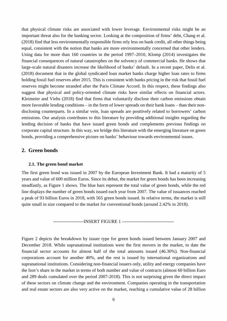
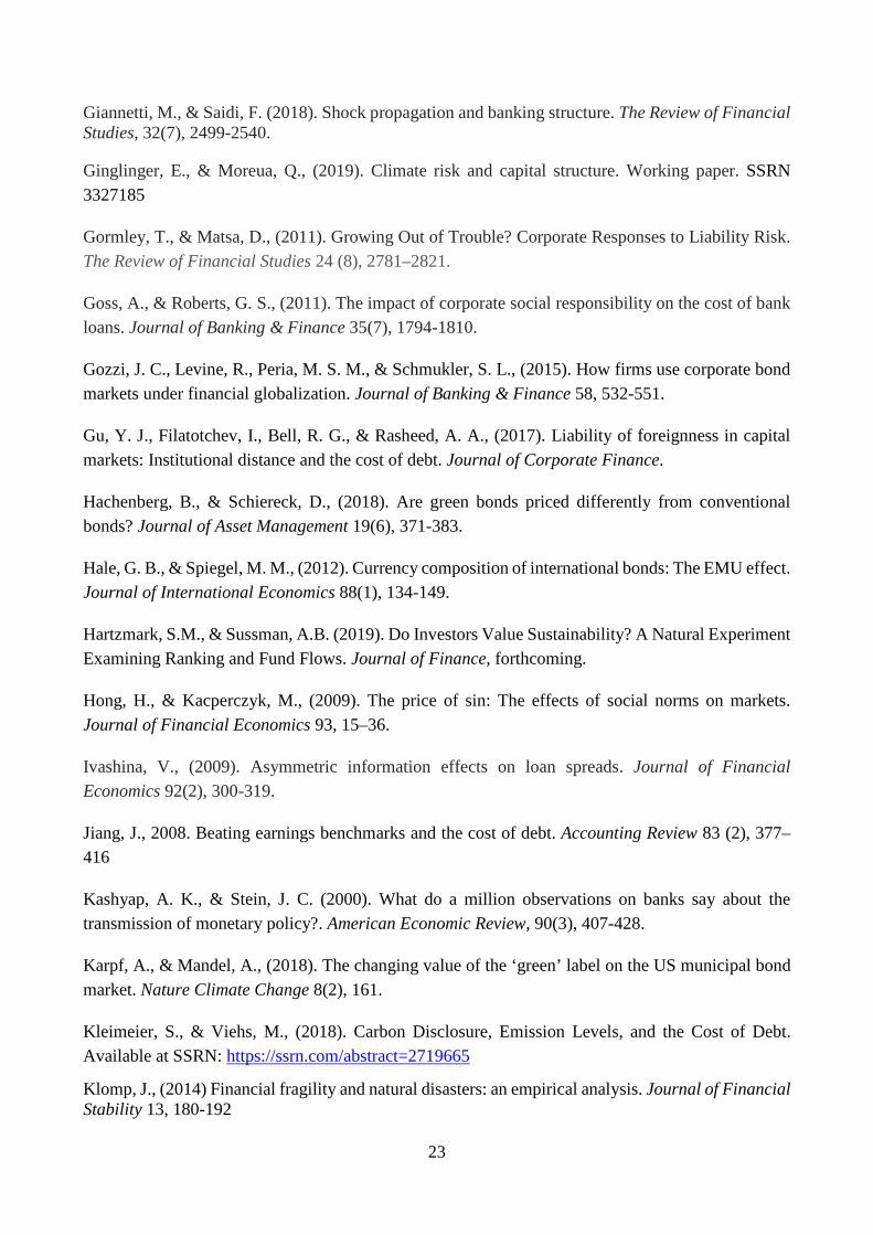
The first green bond was issued in 2007 by the European Investment Bank. It had a maturity of 5 years and value of 600 million Euros. Since its debut, the market for green bonds has been increasing steadfastly, as Figure 1 shows. The blue bars represent the total value of green bonds, while the red line displays the number of green bonds issued each year from 2007. The value of issuances reached a peak of 93 billion Euros in 2018, with 565 green bonds issued. In relative terms, the market is still quite small in size compared to the market for conventional bonds (around 2.42% in 2018).

--------------------INSERT FIGURE 1 ----------------------------------

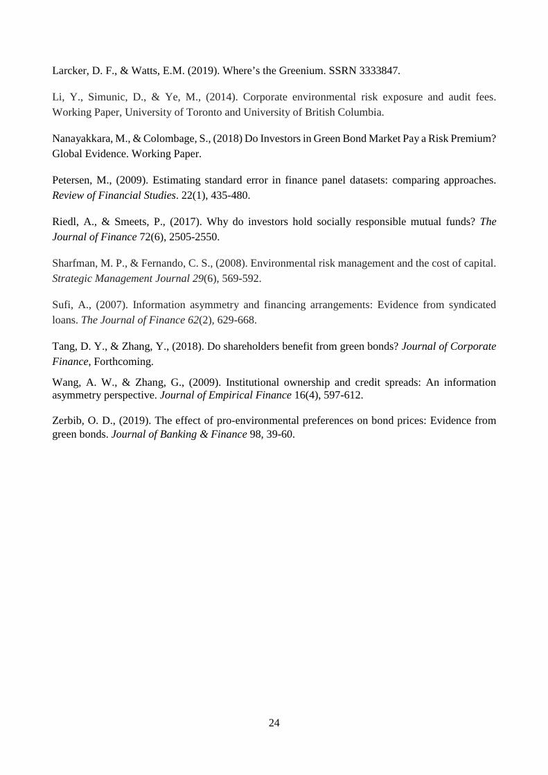
Figure 2 depicts the breakdown by issuer type for green bonds issued between January 2007 and December 2018. While supranational institutions were the first movers in the market, to date the financial sector accounts for almost half of the total amounts issued (46.30%). Non-financial corporations account for another 40%, and the rest is issued by international organizations and supranational institutions. Considering non-financial issuers only, utility and energy companies have the lion’s share in the market in terms of both number and value of contracts (almost 60 billion Euro and 289 deals cumulated over the period 2007-2018). This is not surprising given the direct impact of these sectors on climate change and the environment. Companies operating in the transportation and real estate sectors are also very active on the market, reaching a cumulative value of 28 billion

7

Euros. In terms of contract duration, the data shows a prevalence of short (0-5 years) and medium (5-10 years) term maturities, which combined account roughly for 75% percent of the market value, roughly equally split. The rest of the market comprises long-term contracts with a maturity of more than 20 years.

--------------------INSERT FIGURE 2 ----------------------------------

2.2. Background and issues

Green bonds are intended to encourage sustainable activities by financing climate-related or environmentally friendly projects. As discussed in the introduction, there is no commonly accepted definition of a green bond yet. In practice, some guidance in identifying green bonds is provided by the Green Bond Principles (GBP), voluntary process guidelines put forward by the International Capital Market Association (ICMA).3 Specifically, this standardized procedure encourages transparency and disclosure by focusing on four main areas, namely the use of proceeds, the process for project evaluation and selection, the management of proceeds, and reporting. Currently, the labeling of a bond as ‘green’, while reflecting the broad correspondence with the GBP, de facto could be more or less loosely applied by providers of financial markets data, such as Bloomberg or DCM.

The absence of a commonly agreed definition, as well as of a unique reference framework, has been identified by the European Commission as one of the barriers to the development of the green bond market. In its final report, the EU High-Level Group on Sustainable Finance made several recommendations to promote the development of the green bond market (EU HLEG, 2018). In particular, as a first step, ‘the EU should introduce an official EU Green Bond Standard (EU GBS) and consider an EU Green Bond label or certificate to help the market to develop fully and to maximize its capacity to finance green projects that contribute to wider sustainability objectives.’ The formulation of an explicit definition of green bonds based on a common ‘sustainability taxonomy’ advocated by the EU HLEG would ideally address the uncertainties and areas of concern that may require greater prescription than what is provided by the current voluntary standards. At the same time, it would incorporate the existing best market practice.

Since the primary objective of the standard is to help raise investment in green projects and activities, transparency is a crucial issue to mitigate information asymmetries on the actual environmental sustainability of the projects financed by the debt issuance. In practice, several organizations have started to provide green labels that indicate conformity to particular definitions of green. In this way, they align the incentives of potential investors who value the sustainability aspects of the financial instruments, and those of the issuers. While certification and external review undoubtedly increase transparency and provide a reputational benefit to the issuers, they come at a cost. Whether and to what extent the market prizes this additional financial effort by issuers become then relevant questions to answer in the light of the need of promoting the development of the green bond market. Inspired by Baker et al. (2018), in our empirical exercise we check if external review, in the form of second

3 https://www.icmagroup.org/green-social-and-sustainability-bonds/green-bond-principles-gbp/

8

party opinion or certification, has a significant impact on the pricing of green bonds on the primary market.4

Several jurisdictions worldwide, including China, Hong Kong and Singapore, have put in place incentives schemes to support the development of their green bond market, e.g. by subsidising eligible green bond issuers in obtaining verification. At the same time, a reflection on how to scale up green finance has been initiated by the Network for Greening the Financial System (NGFS), a newly created forum of central banks and supervisors. In this context, the Bank for International Settlements has recently started an open-ended fund for central bank investments in green bonds. Against the background of a rapidly developing market and progressing institutional initiatives, our analysis provides new insights to better understand opportunities and risks in the market for green bonds.

3. Data and summary statistics

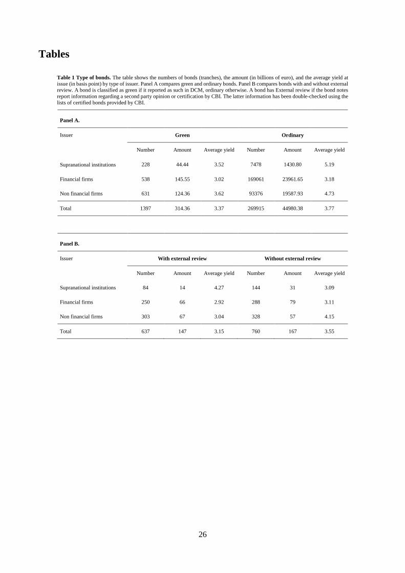
Our main data source is Dealogic DCM, which covers data about bond primary markets worldwide (see e.g. Hale and Spiegel, 2012). DCM provides detailed bond issue characteristics at the tranche level, alongside information about the issuer. We select all bond tranches issued by financial and non-financial companies, as well as supranational institutions in the period 2007-2018.5 Qualitative information on a number of relevant bond characteristics is normally available together with the financial features and other features that are essential in orienting investors’ choices. In the case of green bonds, additional information include the nature of the project for which the proceeds are used, the reporting, and the name of the external reviewer (if any). As a first step in our selection, we consider all the self-labelled green securities. Then, we double-check the qualitative information provided in the tranche note to pin down the bonds for which we have sufficiently detailed information consistent with the self-reported green label.6 We identify 1,397 green bonds out of 271,312 fixed income securities.7

4 External review is a general term that covers a wide spectrum of services from environmental consultancy to audits on use of proceeds. For our purposes, we can include two different types of external review: i) second party opinion; ii) certification. For the latter, we rely on the certification procedure provided by the Climate Bond Initiative (CBI). The CBI's Climate Bonds Standard establishes sector-specific eligibility criteria to judge an asset's low carbon value and suitability for issuance as a green bond. Assets that meet the CBI standard are then eligible for Climate Bond Certification, after an approved external verification that the bond meets environmental standards and that the issuer has the proper controls and processes in place. 5 While also government bodies issue green bond we limit our analysis to financial and non-financial corporations. See Baker et al. (2018) for a study on bond issued by U.S. municipalities. 6 Disclosure of relevant information to the market has been identified as one of the reasons for the increasing popularity of green bonds (Financial Times, 2019). Specifically, transparency on the use of proceeds is of paramount importance. Most market guidelines require that use of proceeds reporting is disclosed at least annually after issuance. Some issuers are also providing information on impact reporting, which is not mandatory in any guidelines, but considered as a best practice, as it strengthens market accountability. We retrieve the information on the use of proceeds applying text mining techniques to the ‘tranche note’ that accompanies each bond tranche. Specifically, we analyse the fields ‘bonds use of proceeds’ and ‘category’. The latter contains information on the detailed investment projects where the funds are allocated. We additionally classify as ‘undisclosed’ the bonds for which there is no description available in the ‘category’ field. 7 An alternative database commonly used in the literature is Bloomberg, which also provides information on green bonds. Dealogic Debt Capital Markets database (DCM) covers the global primary market bond data since 1980, including many details regarding the issuance. We have compared information on green bonds reported by DCM and by Bloomberg. In Bloomberg, the number of unique ISIN numbers associated to green bonds issued worldwide until 31 December 2018 is 1,665. By matching their ISIN codes, we find that both data providers classify 830 bonds consistently as green. They

9

Table 1 shows that the majority of green bond issuances has been made by the corporate sector, with financial corporations having issued the largest cumulative amount so far. This is partially explained by the strong reliance of financial firms on the bond market, on aggregate, compared to the non-financial firms. Looking at the yields, it is apparent that, on average, the green bonds in our sample have a lower yield at issuance than ordinary bonds issued by the same type of borrowers. Exploiting the qualitative information on external review, we identify a total of 637 bonds that have obtained a second party opinion or are certified by the Climate Bond Initiative (CBI). Interestingly, non-financial firms resort to certification more frequently than other issuers. Table 1 shows that bonds with external review have average lower yields than self-labelled green bonds without review. This is particularly true for financial and non-financial firms.

--------------------INSERT TABLE 1----------------------------------

4. Econometric strategy

To investigate the pricing implications of the green label we use a standard equation for bond yields. In particular, we follow Baker et al. (2018) who develop a model of asset pricing with a non-pecuniary clientele in the spirit of Fama and French (2007). In this setup, pro-environment tastes can be accommodated in a straightforward way. Specifically, our econometric model is as follows:

𝑌𝑌𝑌𝑌𝑌𝑌𝑌𝑌𝑌𝑌𝑏𝑏,𝑖𝑖,𝑡𝑡 = 𝛽𝛽0 + 𝛽𝛽1𝐺𝐺𝐺𝐺𝑌𝑌𝑌𝑌𝐺𝐺𝑏𝑏,𝑖𝑖,𝑡𝑡 + 𝛽𝛽2𝑿𝑿𝑏𝑏,𝑖𝑖,𝑡𝑡 + 𝛿𝛿𝑖𝑖 + 𝜙𝜙𝑡𝑡 + 𝜖𝜖𝑏𝑏,𝑖𝑖,𝑡𝑡 (1)

where 𝑌𝑌𝑌𝑌𝑌𝑌𝑌𝑌𝑌𝑌𝑏𝑏,𝑖𝑖,𝑡𝑡 refers to the yield at issuance of bond b issued by issuer i in time t. 𝐺𝐺𝐺𝐺𝑌𝑌𝑌𝑌𝐺𝐺𝑏𝑏,𝑖𝑖,𝑡𝑡 is our main variable of interest, which equals one if a bond is green, and zero otherwise. The vector X includes a set of bond characteristics that may affect the yield. In line with previous literature (see e.g., Gu et al., 2017; Gozzi et al., 2015; Chen et al., 2011), we control for callable, a dummy variable which is equal one if a bond is callable, zero otherwise; puttable a dummy variable which is equal to one if a bond is puttable, zero otherwise; and collateralized a dummy variable which is equal to one if a bond has some underlined collateral, zero otherwise. Furthermore, we control for the currency of issuance and the purpose of a bond, through the variable use of proceeds, distinguishing between general corporate purposes, securitization, refinancing, and any other use. We create decile categories both for the size of the tranche and the total amount borrowed by the issuer on that day. Maturity is a categorical variable that distinguishes among short-term (less than five years), medium-term (between five and ten years) and long-term (more than ten years) bonds. We also consider the bond rating, as provided by S&P, Moody’s or Fitch, and define eleven categories with 1 assigned to the

account for 70% of the green amounts in DCM. Among the unmatched securities, 32% (266) of green bonds in Bloomberg are considered as conventional bonds in Dealogic DCM. Overall, we rely on the latter data as it provide more detailed qualitative information on bond features which are useful to double check the green label, e.g. information on the use of proceeds, on the reporting by the issuer, certification, verification and/or second party opinion, including the name of the reviewer.

10

top rating and 11 to the worst rating (or not rated). Further, time fixed effects are introduced to capture global time-varying unobservable factors that might affect the primary bond market in a specific month. We adopt a conservative approach and include the interaction fixed effect maturity×rating×time to account for twists in the yield curve. We control for time-invariant unobservable firm-specific characteristics using an issuer fixed effect, 𝛿𝛿𝑖𝑖. Finally, 𝜖𝜖𝑏𝑏,𝑖𝑖,𝑡𝑡 is the error term. In the regression we cluster standard error at the issuer level to address potential issues stemming from residuals correlation (Petersen, 2009). Table 2 reports the summary statistics for the variables used in the bond pricing analysis.

--------------------INSERT TABLE 2----------------------------------

5. Results

5.1. Main results

Table 3 reports our baseline results. Column (1) displays the results for the full sample comprising all categories of borrowers. The coefficient of the green dummy is negative, suggesting that green bonds sell for a moderate premium over ordinary bonds. However, the effect is not statistically significant. The analysis of the overall sample may hide some heterogeneity in the way different types of issuers – particularly financial and non-financial borrowers – access the bond market, and are ultimately evaluated by investors. We account for such heterogeneity by running separate regressions for the different categories of issuers in our sample, namely supranational institutions, financial and non-financial corporations. The results are reported in columns (2)-(4) of Table 3. The coefficient estimates vary significantly across issuer types. First, we find that only green bonds issued by supranational institutions (column (2) of Table 3) and non-financial corporations (column (4)) sell for a premium compared to ordinary bonds. At 80 basis points, the yield gap for supranational institutions, highly statistically significant, is almost four times larger in magnitude than that for non-financial corporations. By contrast, we do not find a statistically significant yield difference for green bonds issued by financial institutions (column (3) of Table 3).

A discussion on the size of the estimated greenium(s) is in order. Let us first focus on corporates, for which we find a yield gap of around 22 basis points in favour of green bonds. To put that in perspective, let us first recall from Table 1 that, in our sample, the average yield of corporate green bonds is 3.6%. Then, the estimated gap is only around 5% (22/473=4.6%) of the average yield of conventional bonds issued by corporates. A meaningful comparison with existing studies is hampered by the sheer heterogeneity in samples and methodologies used in the literature.8 Prima facie, the 80 basis point premium in favour of supranational institutions might strike as very large. However, such order of magnitude is not surprising if one considers the strong reputational advantage of these issuers. Supranational institutions were indeed the very early (and, for some years, only) movers in

8 As a comparison, Baker et al. (2018) using a similar empirical framework find a premium of 6 basis points, which is roughly 2.6% of the average after-tax yield of AAA conventional bonds. In their sample they consider a different type of issuers.

11

the green bond market. Therefore, their role in the green segment is well established. In addition, the very nature of their purpose, i.e. to promote sustainable development, instead of pure profit maximization, minimizes concerns that the issuance of green bonds is pure greenwashing to attract investors. If investor preferences drive the market premium, the risk of greenwashing might indeed hold back green-minded investors from massively demanding securities issued by the corporate sector, but not those issued by supranational institutions. This might explain the differences in the estimated greeniums.

--------------------INSERT TABLE 3 ----------------------------------

If investors have preferences for green products, asymmetric information on the greenness of the underlying projects is crucial for preferences to affect market prices.9 Are there ways in which issuers can signal their genuine commitment to green activities? We shed light on this issue in two alternative ways. First, we test whether external review has an impact on the offering yield. If external review acts as a signalling device for bonds that actually have environmental or climate-related benefits, we expect certified bonds to sell for a premium compared not only to conventional bonds but also to non- green securities. Operationally, we augment the baseline model with a dummy variable (External review) that takes the value of one for green bonds that are CBI-certified or have obtained a second party opinion, and zero for self-labelled green securities. Table 4 reports the results for the full sample and for the sub-samples for homogeneous issuer types. The review dummy does not affect the average bond yield in the full sample (column (1)). The sample splitting exercise sheds light on the drivers of these findings. First, due to lack of observations, we are not able to identify the effect of external review on the issues of supranational institutions (column (2)). Second, we find again a marked difference between financial and non-financial issuers. The coefficient of the review dummy is not significantly different from zero for financial green bonds (column (3). By contrast, as expected, it is negative for bonds issued by non-financial corporations (column (4)), where it is statistically significant al 5%. At almost 44 basis points, the estimated impact of external review is sizable, particularly if compared with the effect of the self-reported green label 21 bps. Interestingly, this latter is not estimated with precision in the augmented model.

Alternatively, we consider repeated debt issues on the green bond market as a way to provide information benefits to investors. Accordingly, we augment our baseline model with the dummy variable Experienced green, which is equal one if the issuer has already placed a green bond, and zero otherwise. If multiple green bond issuances give investors an increasing engagement with borrowers’ business, then we would expect returning issuers to benefit from a correspondingly larger ‘greenium’ than first-time bond sellers. The results of the augmented model are reported in Table 5. In the full sample, the coefficient of the dummy for returning issuers is negative and statistically significant at 10% (see column (1)). The magnitude of the effect is around 44 bps. Again, the breakdown by issuer categories reveals some heterogeneity in the effects of greenness. In particular, 9 Riedl and Smeets (2017) show that individual investors are willing to give up financial performance in order to invest in accordance with their preferences. They investigate social responsible investments but it is likely that these results may apply as well to green products following the increasing concerns for global warming.

12

supranational and financial institutions that have already resorted to the green bond market do not benefit from a ‘greenium’ on their subsequent issuances (see columns (2) and (3)). By contrast, this is the case for non-financial corporations (column (4)). The negative yield gap with respect to one-time issuers is around 35 bps. One explanation could be that issuers placing more than one green bond are able to better signal their greenness over time. The build-up of a reputation and/or a better ability to screen borrowers on the part of investors might indeed explain the premium we find in favor of returning non-financial issuers. From the borrowers’ perspective, the premium associated with multiple issuances might be justified by the additional disclosure costs that returning to the green bond market entail for borrowers.

--------------------INSERT TABLE 4 ----------------------------------

--------------------INSERT TABLE 5 ----------------------------------

5.2. Robustness analysis

In this section, we provide a battery of tests to check the robustness of the negative relationship between yield to maturity and the green label. Our baseline regression model in equation (1) includes issuer fixed effects that, together with rating fixed effects, control for issuer characteristics which might affect bond yields. In line with previous literature (see e.g. Gu et al., 2017; Gozzi et al., 2015; Chen et al., 2011), we extend our baseline specification adding a number of issuer-specific variables, which capture relevant features such as credit risk, profitability and liquidity risk.10 In particular, we include the following variables. Size is the natural logarithm of the book value of total assets (in millions of Euro). Leverage is the ratio of debt to the book value of total assets. Profitability is the ratio between operating income before depreciation and the book value of total assets. As a proxy for firm liquidity, cash ratio is defined as cash over the book value of total assets. Equity volatility is calculated by annualizing the daily volatility of stock returns in the previous 180 days. Table 6 presents the regression results.11 Similarly to the evidence in Table 3, we do not find an effect for the green label when considering both the overall sample and financial issuers (columns 1 and 2). While, for the subsample of corporate issuers the coefficient for the green bond is negative and statistically significant (column 3).

A concern with our analysis is that the issuance of green bonds may correlate with unobservables that also affect the yield. Indeed, companies do not randomly issue green bonds, which may raise endogeneity concerns if firms that have lower bond yields are also those issuing green securities. Ideally, we would like to find an instrument for green bond issues to address this concern. However, it is hard to come up with an adequate variable allowing for an IV approach. Instead, we adopt a matching procedure whereby we pair green issuers to similar non-green issuers (‘control issuers’) 10 Firm financial data are retrieved from Bloomberg. We use ISIN codes to match bonds in DCM with the corresponding securities in Bloomberg. 11 Due to limited data availability, the sample is considerably reduced. It includes financial and non-financial issuers only, and issuers headquartered in the following countries: EU28, United States, Australia, Canada, Japan, Malaysia. Summary statistics are reported in Table 14 in the Appendix.

13

based on a set of covariates. We first restrict the eligible control issuers to have issued a bond in the same year, to operate in the same industry and in the same country. Then, within the pool of potential control units, we select those most similar to the green bond issuers based on observable characteristics, such as size, leverage and profitability, using a nearest neighbor procedure. Thus, by removing meaningful differences along observable dimensions, we make sure that the control issuers are as similar as possible to the green issuers (see Table 15 in the Appendix). In this way, we reduce potential concerns that issuer characteristics that affect the decision to issue a green bond are determined also by the estimated yield gap between green and conventional securities. The estimates are presented in Table 7. While the matching approach considerably reduces the sample, our main results are confirmed.

Third, we check whether our baseline results are robust across different samples and sub-samples. In Table 8 panel A, we investigate whether the country of the issuer matters for the existence and the magnitude of the ‘greenium’, ceteris paribus. In particular, we distinguish between emerging and developed countries, for the full sample of all borrowers as well as for the sub-samples of homogeneous issuer types. All in all, the estimates suggest that the results of the baseline model are mainly driven by supranational and non-financial issuers located in developed economies.12 In Panel B of Table 8, we check the effect of the currency denomination on the offering yield of the bond. Previous literature has found that bonds denominated in local currency tend to have a tighter credit spread because they hold a lower exchange risk than bonds issued in foreign currencies, ceteris paribus (Ehlers and Packer, 2017; Nanayakkara and Colombage, 2018). To test for this, we create a dummy variable (labelled Local) equal to one if the bond is denominated in local currency, and zero otherwise. While the effects of the local currency dummy are borderline statistically significant only in the full sample with all issuers, the results for the green label are not quantitatively different from those in the baseline model in Table 3.

As a further robustness check, we adopt a different definition of the dependent variable. So far, our left hand variable has been the offering yield of the bond in the primary market. Such yield reflects the risk premium that issuers pay to investors to raise funds. Following previous studies (Jang, 2008; Ge and Liu, 2015; Shi, 2003; Wang and Zhang, 2009), we alternatively measure the dependent variable as the difference between the bond yield at issuance and a sovereign bond yield with comparable maturity, issued in the same country as our reference security.13 This allows us to filter the bond credit risk from the associated sovereign risk. In other words, the yield spread is a direct and accurate measure of issuers’ incremental cost of a bond over a comparable risk-free government bond. In addition, by taking the difference between the returns, we also control for the effect of economy-wide factors that might affect bond yields. Constrained by the thickness of sovereign bonds markets, we perform this robustness analysis only for OECD countries. Overall, we cover 70% of our initial sample of bond issuances. The first two columns in Table 9 report the results. For the sake of comparison, columns (3) and (4) display the estimates of the baseline model with the offering yield 12 We do not need to control for country fixed effects (or industry fixed effects) as these are absorbed by - the issuer fixed effects that we include in our baseline specification. 13 We match our sample with the sovereign bonds dataset downloaded by Dealogic DCM. We used the propensity score matching algorithm to find comparable Treasury bonds. Once selected the country of the issuer we define the set of associated sovereign bonds and successively we run the algorithm in order to find the closer sovereign bonds, computing the distance based on Issuance date and time to maturity.

14

as the dependent variable on the sub-sample of issuers located in OECD countries. The results for the yield spread are in line with those for the baseline model. In particular, we find a non-negligible and statistically significant green bond premium in favor of non-financial corporate issues compared to conventional bonds.

--------------------INSERT TABLE 6 ----------------------------------

--------------------INSERT TABLE 7 ----------------------------------

--------------------INSERT TABLE 8 ----------------------------------

--------------------INSERT TABLE 9 ----------------------------------

5.3. Green bonds and financial institutions

The analysis in the previous sections suggests that there are significant differences in how the market prizes the green label across types of issuer. In particular, while we find a significant ‘greenium’ for non-financial corporations, there is no evidence of a similar price advantage for green bonds issued by financial institutions, ceteris paribus. Why does the ‘greenium’ materialize only for some categories of issuers, but not for financial companies? One possible reason behind such heterogeneity is that while non-financial companies may signal the greenness of the projects for which the bond proceeds are used in a more transparent way, this may be more difficult for financial institutions. This might stem from the very nature of the type of business. Non-financial corporations normally issue green bonds to finance environmental or climate-related projects. As such, they can easily detail the activities that the bond proceeds are earmarked to finance, and further commit to report details during the lifetime of the bond. While the link with green projects is immediate for non-financial corporations, this is not necessarily the case for financial institutions, whose alignment with environmental/climate principles might be more difficult to signal to the market. Alternatively, activity on the green bond market might be motivated by the informational advantage that can be obtained therein and used in future underwriting procedures. In general, mitigation the information asymmetry on the use of funds to rule out greenwashing might be more difficult for financial issuers. As an indirect way to test for the importance of signalling greenness, we consider membership in the United Nations Environment Programme Finance Initiative (UNEP FI) as a proxy for banks’ attitude toward environmental and climate change issues. The United Nations Environment Programme Finance Initiative (UNEP FI) is a global partnership between the United Nations and the financial sector, established with the aim to encourage the better implementation of sustainability principles at all levels of operations in financial institutions.14 We define a dummy variable (labelled Environmentally friendly) taking the value one from the year onward in which a bank signed the initiative, and zero otherwise. Then, we augment our baseline specification with this variable dummy and its interaction with the dummy Green. Provided membership in the UNEP FI correctly signals a

14 Over 200 members (banks, insurers, and fund managers) have joined the initiative. Data are taken from http://www.unepfi.org/members/

15

business strategy aligned with environmental objectives, we expect a negative coefficient for the interaction term. The results are reported in Table 10. Indeed, we find that green bonds issued by financial institutions affiliated to the UNEP FI benefit from a price advantage compared to financial issuers that have not subscribed to it.

--------------------INSERT TABLE 10 ----------------------------------

6. Financial issuers and green lending

In this section, we investigate the lending behaviour of financial institutions that have issued green bonds with the aim to provide further insights on our previous results. The analysis on green bond pricing has documented that, while a significant amount of green bonds are issued by financial institutions, there is no evidence of a pricing advantage of financial green bonds compared to ordinary bonds, ceteris paribus. Compared to non-financial issuers, investors may account for the higher degree of information asymmetry on the use of funds raised by financial issuers when issuing a green bond. For financial issuers, there are inherent difficulties in tracing the proceeds of the bond to specific green projects. Likely, the link is only indirect whenever the green bond funding finds a correspondence in a green portfolio on the asset side of banks’ balance sheets. Thus, it is more difficult to credibly signal the commitment to support environmentally friendly activities to the market. In section 5.3 we provide evidence of a positive effect when there is a credible signal. In this section, we focus instead on bank lending behaviour, and test whether green issuers in the financial sector shift their lending towards less polluting activities after issuing a green bond. To this end, we combine information on syndicated loans with data on sectoral pollution intensity exploiting information on the economic activity and location of the borrowing companies. In an ideal setting, we would like to observe more details regarding the loans – for example, details on the projects financed in each loan – allowing us to identify “green loans”, which would be eventually associated to the green bonds issued (i.e. amounts, maturity…). Unfortunately, we face significant data constraints. First, we do not have loan data at the project level to precisely trace the use of funds. Second, while some information on green loans is currently available, the data are scant and their quality needs to be carefully verified. Moreover, the classification of loans as green is not based on commonly accepted standards. With these constraints in mind, we believe our analysis is nonetheless informative in that it provides some insights about the role of the banking sector in funding green activities. While the green bond market is playing an important role in financing green projects, a significant number of firms, particularly in Europe, does not have access to the bond market but relies mainly on the banking sector as a source of external funding.

16

6.1. Data

We draw data on syndicated loans from DealScan.15 We can rely on a rich information set where we can identify the borrower and lenders at origination, as well as the main characteristics of the loan. To start with, we consider the sample of loans extended to European companies in the period 2007-2018.16 We retrieve 37,488 syndicated loans. We include only loans with full information on the size of the deal, the nationality of borrowers involved and some other basic deal characteristics. In a syndicated loan usually more than one bank provides funding. The lead arrangers set the terms of the deal and a preliminary agreement is signed. After the due diligence, the lead arrangers recruit other participant lenders to provide part of the funds. Finally, the loan contract is signed. To identify the lead bank in each loan, we follow previous literature (see, e.g. Ivachina 2009, Acharya et al. 2017) and consider the definitions suggested by Standard & Poor’s, which for the European loan market are ‘mandated lead arranger’, ‘mandated arranger’, or ‘bookrunner’. Having identified the lead lenders and the other deal participants, we use the information about the deal structure to fill in those loan shares that are missing.17 This procedure allows us to compute for each deal the lending amount of each bank. Then, we manually match the lenders in the sample of loans with the financial institutions issuing bonds. We are left with 34,852 loan contracts, corresponding to 222 unique banks. By merging these two datasets, we can identify the banks that have issued green bonds and, at the same time, observe their pre- and post-issuance lending behavior. Accordingly, we define the dummy variable Green_issuer, which is equal to one from the time t when a bank that has issued a green bond onwards, and zero otherwise.

As a measure of the ‘brownness’ of the activities against which we evaluate banks’ lending behavior, we use data on greenhouse gas – that is CO2 plus other air pollutants expressed in CO2 equivalent –emissions intensities. The data, obtained from Eurostat, contains information on greenhouse gas emissions at annual frequency (2007-2017), broken down by country and 64 industry (NACE Rev. 2 activity).18 We consider air emission intensities expressed as the ratio between greenhouse gasses and a measure of economic activity, expressed in terms of value added or output. Emission intensities are in kilograms per euro. Larger values are associated with more polluting activities. We match these data with the loan data using the information on the industry and the country of the borrower company. As a final step, for each bank, we aggregate the lending volumes extended to each industry-country pair in all periods.

15 While syndicated lending is only a fraction of banks’ total lending, it is commonly used to evaluate bank lending policies and their impact on the real economy (e.g., Chodorow-Reich, 2013; Acharya et al., 2018). 16 We consider companies located in the countries for which Eurostat provide greenhouse gas emission data, namely EU member states, EFTA countries and candidate countries. 17 Specifically, we follow the approach of Chodorow-Reich (2013). We take the average of the actual loan shares for lead and participant banks for all deals with the same syndicated structure (number of lead and participant banks). Then, we impute this information when the loan shares are missing to those loans with the same structure. 18 To the best of our knowledge, the Air emissions accounts (AEA, Eurostat) is the most disaggregated level to which green gasses emissions are available with a supply-side sectoral breakdown. Alternative datasets provide data at the country level only (i.e. Germanwatch, Worldbank). Unfortunately, despite an improvement in disclosure practices, firm-level data on carbon emissions, are available only for a very limited number of firms (see e.g. Carbon Disclosure Project).

17

6.2. Econometric specification

To investigate whether banks reduce their lending to more polluting industry-country pairs after the issuance of a green bond, we use the following regression:

𝑌𝑌𝑏𝑏𝑏𝑏𝑏𝑏𝑡𝑡 = 𝛼𝛼 + 𝛽𝛽𝐺𝐺𝐺𝐺𝑌𝑌𝑌𝑌𝐺𝐺_𝑌𝑌𝑖𝑖𝑖𝑖𝑖𝑖𝑌𝑌𝐺𝐺𝑏𝑏𝑡𝑡 + 𝜆𝜆Emission_intensities𝑏𝑏𝑏𝑏𝑡𝑡

+𝛾𝛾𝐺𝐺𝐺𝐺𝑌𝑌𝑌𝑌𝐺𝐺_𝑌𝑌𝑖𝑖𝑖𝑖𝑖𝑖𝑌𝑌𝐺𝐺𝑏𝑏𝑡𝑡 × Emission_intensities𝑏𝑏𝑏𝑏𝑡𝑡 + 𝑖𝑖𝑏𝑏𝑏𝑏𝑏𝑏𝑡𝑡.

(2)

The dependent variable (𝑌𝑌𝑏𝑏𝑏𝑏𝑏𝑏𝑡𝑡) is the total loan volume that industry j in country c attains from bank b in period t (expressed in logarithms).19 𝐺𝐺𝐺𝐺𝑌𝑌𝑌𝑌𝐺𝐺_𝑌𝑌𝑖𝑖𝑖𝑖𝑖𝑖𝑌𝑌𝐺𝐺 is a dummy variable that equals one from the time t the bank b has issued a green bond onwards, and zero otherwise. Emission intensities is the ratio between greenhouse gasses and the output for a specific industry j in country c in period t. The parameter 𝜆𝜆 captures how the emission intensities of a specific industry-country affect the amount of lending. The parameter of interest, 𝛾𝛾, provides an indication of the lending activities of banks after having issued a green bond in relation to the pollution intensity. A negative coefficient estimate would indicate that banks increase their lending towards those industry-country polluting less.

The specification includes also a full battery of fixed effects defined by the pairwise interactions for bank×industry, bank×country, and bank×year. The former two sets of fixed effects capture the specialization or proximity of a bank to a specific industry or country. The bank-year fixed effects saturate the regressions from other supply factors. We address concerns related to demand factors using industry×country, country×year and industry×year fixed effects. Our empirical strategy is similar to the one proposed by Giannetti and Saidi (2018). They investigate whether lenders provide larger loans to industries in distress using a specification at bank-industry-year level. We have a richer setup since we can exploit also variability at the country level. Thus, we can include a wider set of interaction terms to control for any factor that might lead to a spurious correlation between the bank lending of green issuers and emissions.

In an alternative specification, we include bank-specific variables to control for determinants of bank lending on the supply side. Following the literature on bank lending behaviour (see e.g., Kashyap and Stein, 2000), we include the log transformation of a bank’s total assets to capture bank’s size. We control for a bank’s capital structure by including the capital ratio, defined as equity over total assets. Further, the bank’s funding structure is captured by the ratio of long-term funding over total liabilities. Bank profitability is proxied by the EBIT over total assets, while the ratio between impaired loans and equity provides a measure of the fragility of the loan portfolio relative to the bank's capital. Bank-level data are retrieved from the Bank Focus dataset provided by Bureau van Dijk. In addition, we control for relevant factors affecting credit demand using country and industry specific controls. As for the former, we include GDP per capita and GDP growth to control for the business cycle. Both variables are taken from the World Bank WDI dataset. To capture any structural difference in the borrowing propensity at the industry level, we consider leverage (the ratio of debt over total assets), the liquidity ratio (cash over total assets), a measure of intangibility as the ratio of intangible assets over total assets, and the profitability ratio (the ratio of EBIT over total assets). To construct these 19 Alternatively, we use an indicator for whether the lender serves as participant in the syndicated loan as our dependent variable. Our specification follows Giannetti and Saidi (2018).

18

variables we use firm-level information from the ORBIS dataset compiled by Bureau van Dijk. We first compute each ratio at the firm level using unconsolidated balance sheets, then we calculate the median value for each industry-country-time.

Summary statistics of our main variables are displayed in Table 11. We limit the sample to bank-industry-country (bjc) with non-zero loans in at least two years. We end up with 35% of the observations that are associated with positive loans. The variable green issuer is equal to one for only 15% of the observations (51 banks in our matched sample issued at least one green bond in the period 2007-2018). Emission intensities are on average equal to 0.63 Kg per euro, but with a significant variation across both industries and countries. Summary statistics for the additional variables are reported in the Appendix (Table 18).

--------------------INSERT TABLE 11 ----------------------------------

6.3. Results

We report our main results in Table 12. Columns (1)-(3) refer to the full sample while in columns (4)-(6) we exclude domestic lending, defined as the lending of bank b to a borrower headquartered in the same country c of the lender. The models in columns (1) and (4) bank, industry, country and year fixed effects. In columns (2) and (5) we add bank, country, industry and year controls, and bank×industry, bank×country. While in columns (3) and (6) we include the full set of interaction fixed effects discussed above, which control for confounding factors, both on the demand and on the supply side of the market, that might potentially threaten identification. The results for our baseline model with the (logs of) the loan size as the dependent variable are reported in panel A of Table 12. In all specifications, the negative coefficient estimated for the variable Emission_intensities suggests that larger emission intensities are associated with a lower amount of lending. Importantly, also the interaction term between Green_issuer and Emission_intensities is negative and statistically significant in all models.20 This means that an increase in emission intensities yields a relatively larger reduction of lending volumes by banks that have issued green bonds. While the nature of our data prevents us from drawing conclusions on the specific use of green bond proceeds to finance less polluting projects, we can nonetheless conclude that financial green bond issuers are committed to shifting their lending away from more polluting activities. In terms of magnitude, the specification in column (3) implies that a one standard-deviation increase in the emission intensities yields a 10% reduction of lending volumes by banks active on the green bond market. The effect carries over when domestic loans are excluded from the sample (columns (4) and (6)). In panel B we use the average amount granted to industry j in country c by bank b, instead of total loan volumes, as our dependent variable. The results are not quantitatively different from those in panel A, suggesting that the effect in the baseline specification is not driven by a limited number of large deals. We further explore whether the negative impact of emission intensities on lending, following a green bond issuance, persists also at the extensive margin. In panel C the dependent variable is a dummy variable that takes

20 In columns (2) and (4) the dummy Green_issuer drops due to multicollinearity.

19

the value of one if bank b has extended any loan to industry j in country c in period t, and zero otherwise. The interaction term between Green_issuer and Emission_intensities is still negative and statistically significant. Thus, not only the amount of the loans, but the very same decision to lend to sectors and countries with relatively high levels of greenhouse gas emissions change after the emission of a green bond. These findings suggest that, after having issued a green bond, banks lower their lending towards more polluting activities. These evidence complement previous results showing that firms with larger environmental risks have lower leverage level (Chang et al., 2018; Ginglinger and Moreau, 2019).

--------------------INSERT TABLE 12 ----------------------------------

In Table 13 we provide additional robustness tests for our lending model. The first three columns report the results for the full sample, with different sets of fixed effects and control variables. The results in columns (4)-(6) refer to the sub-sample of loan contracts extended to foreign borrowers. In panel A, we redefine the dependent variable as the total amount granted by bank b independently of its role in the syndicate, i.e. when acting as participant or lead bank. Interestingly, our baseline results carry over for both samples with the set of bank, country, industry and year dummies as well as with bank, country and industry controls. However, in the most conservative set up with the full set of interaction fixed effects (columns (3) and (6)) the negative coefficient of our variable of interest is statistically insignificant. This implies that banks do not change their overall lending decisions based on the degree of greenness of the borrowing sector after having issued a green bond. A reason for that might be found in the fact that banks participate in syndicated loans because of motivations other than the pure lending decision, for instance to establish or maintain a relationship with other syndicate members (Sufi, 2007). The result also suggests some caution in interpreting the results for the lead banks. In panel B, we replicate the baseline regression using a different definition of emission intensities computed as the ratio of gas emissions over output. The results are in line with those in the baseline model. As an additional robustness check, in panel C we exclude public sector bodies and financial institutions from the pool of borrowers, as these sectors are commonly excluded in evaluating bank lending policies. In panel D we exclude loans granted to finance mergers and acquisitions. In this way we rule out the possibility that our results are only driven by borrowers in need of extra-funding. All the results are qualitatively similar to our baseline findings. Finally, in panel E we replace the continuous variable measuring emission intensities with a dummy variable (Climate-policy-relevant) which takes value one if industry j is considered relevant to climate mitigation policies. To this purpose, we adopt the taxonomy in Battiston et al. (2017) who map economic activities using the NACE Rev. 2 (4 digits) classification based on their relevance to climate mitigation policies. In this way they are able to estimate the impact of climate risks on the financial system through its exposure to specific sectors. Thus, we consider borrowers’ economic activities and we construct the variable Climate-policy-relevant, and then the interaction term Green issuer×Climate-policy-relevant. Models in columns (1) and (4) include bank, country and industry controls only. In columns (2) and (5) we add bank, industry, country and year fixed effects. In columns (3) and (6) we control for lender specific preferences including also bank×industry,

20

bank×country fixed effects. The coefficient of the variable Climate-policy-relevant is negative, suggesting that economic activities that impact more on climate change received a lower volume of lending, everything else equal. Our parameter of interest, the coefficient of the interaction term, achieves statistical significance at 1% level only in models (1) and (4), while in model (2) and (3) it is statistically significant at 5% and 10%, respectively. By adding a larger set of fixed effects, being the variable dichotomous, the identification power is reduced. Still, the negative sign in all specifications provides evidence consistent with our previous results.

--------------------INSERT TABLE 13 ----------------------------------

7. Conclusions

Green bonds are a major market-based solution to channel funds into environment friendly activities and projects. While relatively new, the market is developing steadfastly. In this paper we investigate the pricing implications of the green label at issuance for non-governmental borrowers. Moreover, we test whether external review and repeat issuance have further impacts on equilibrium prices. We find that, after controlling for relevant characteristics of the debt instruments, green bonds issued by supranational institutions and non-financial corporates indeed benefit from a premium compared to ordinary bonds. This suggests that companies with high environmental performance benefit from a lower cost of debt. Furthermore, we find that green bonds with external review benefit from a larger premium compared to self-labelled green securities. This corroborates the prior that external review is indeed important in this emerging market. While we cannot explicitly elicit investors’ preferences for environment friendly investment from these findings, this is likely the channel at play in our setting. We investigate whether there is a premium in favor of repeat issuers. Indeed, we find that repeat issuers benefit from an additional premium compared to one-time green borrowers, which we take as evidence of a reputation effect on the green bond segment.

While financial institutions raise significant amounts via green bonds, there is no evidence that they benefit from a pricing advantage with respect their ordinary bond instruments, ceteris paribus. We contend that this might be due to the inherent difficulties of linking directly the issuance of a bond with specific green projects. Motivated by the heterogeneity in the effect of the green label on securities offered by different types of corporate issuers, in the second part of the paper we investigate the lending behavior of banks that have used the green bond market. Specifically, we investigate whether financial institutions shift their syndicated lending towards less polluting activities after issuing a green bond. We find evidence that financial green bond issuers reduce their lending to sectors with larger emission intensities. Thus, our analysis highlights that both sides of banks’ balance sheets are becoming to some extent greener. Ultimately, this implies a changed risk profile of banks’ balance sheets, particularly through the direct and indirect exposure to environmental and climate-related risks. While climate change is well recognised as a major challenge to financial stability and the global economy in international fora, such as G20 and the Financial Stability Board, it is still under discussion how micro- and macro-prudential supervision should account for these risks,

21

particularly lower capital risk requirements for green assets. Such regulatory changes would clearly have spillover effects on the green bond market. Future research might address these issues.

22

References Acharya, V. V., Eisert, T., Eufinger, C., & Hirsch, C., (2018). Real effects of the sovereign debt crisis in Europe: Evidence from syndicated loans. The Review of Financial Studies 31(8), 2855-2896.

Baker, M., Bergstresser, D., Serafeim, G., & Wurgler, J., (2018). Financing the Response to Climate Change: The Pricing and Ownership of US Green Bonds. National Bureau of Economic Research.

Barber, B. M., Morse, A., & Yasuda, A., (2018). Impact investing. Working paper. SSRN 2705556.

Battiston, S., Mandel, A., Monasterolo, I., Schütze, F., & Visentin, G., (2017). A climate stress-test of the financial system. Nature Climate Change 7(4), 283.

Chang, X. S., Fu, K., Li, T., Tam, L., & Wong, G., (2018). Corporate environmental liabilities and capital structure. Working paper.

Chava, S., (2014). Environmental externalities and cost of capital. Management Science, 60(9), 2223-2247.

Chen, T. K., Liao, H. H., & Tsai, P. L. (2011). Internal liquidity risk in corporate bond yield spreads. Journal of Banking & Finance, 35(4), 978-987.

Chodorow-Reich, G., (2013). The employment effects of credit market disruptions: Firm-level evidence from the 2008–9 financial crisis. The Quarterly Journal of Economics, 129(1), 1-59.

Climate Bonds Initiative (2017) Green bonds highlights 2016. https://www.climatebonds.net/files/files/2016%20GB%20Market%20Roundup.pdf

Delis, M. D., de Greiff, K., & Ongena, S., (2018). Being Stranded on the Carbon Bubble? Climate Policy Risk and the Pricing of Bank Loans. Working paper.

Ehlers, T., & Packer, F., (2017). Green bond finance and certification. Bank Int. Settlements Quarterly Review.

EU HLEG (2018). Final Report by the High-Level Expert Group on Sustainable Finance.

Fama, E. & French, K., (2007). Disagreement, tastes, and asset prices. Journal Financial Economics 83, 667–689.

Financial Times (2019). Disclosure is a lure for green bond investors. January 30.

Flammer, C., (2018). Corporate green bonds. Working paper. SSRN 3125518.

Ge, W., & Liu, M., (2015). Corporate social responsibility and the cost of corporate bonds. Journal of Accounting and Public Policy, 34(6), 597-624.

Ghoul, S., Guedhami, O., Kwok, C. C., & Mishra, D. R., (2011). Does corporate social responsibility affect the cost of capital? Journal of Banking & Finance 35(9), 2388-2406.

23

Giannetti, M., & Saidi, F. (2018). Shock propagation and banking structure. The Review of Financial Studies, 32(7), 2499-2540.

Ginglinger, E., & Moreua, Q., (2019). Climate risk and capital structure. Working paper. SSRN 3327185

Gormley, T., & Matsa, D., (2011). Growing Out of Trouble? Corporate Responses to Liability Risk. The Review of Financial Studies 24 (8), 2781–2821.

Goss, A., & Roberts, G. S., (2011). The impact of corporate social responsibility on the cost of bank loans. Journal of Banking & Finance 35(7), 1794-1810.

Gozzi, J. C., Levine, R., Peria, M. S. M., & Schmukler, S. L., (2015). How firms use corporate bond markets under financial globalization. Journal of Banking & Finance 58, 532-551.

Gu, Y. J., Filatotchev, I., Bell, R. G., & Rasheed, A. A., (2017). Liability of foreignness in capital markets: Institutional distance and the cost of debt. Journal of Corporate Finance.

Hachenberg, B., & Schiereck, D., (2018). Are green bonds priced differently from conventional bonds? Journal of Asset Management 19(6), 371-383.

Hale, G. B., & Spiegel, M. M., (2012). Currency composition of international bonds: The EMU effect. Journal of International Economics 88(1), 134-149.

Hartzmark, S.M., & Sussman, A.B. (2019). Do Investors Value Sustainability? A Natural Experiment Examining Ranking and Fund Flows. Journal of Finance, forthcoming.

Hong, H., & Kacperczyk, M., (2009). The price of sin: The effects of social norms on markets. Journal of Financial Economics 93, 15–36.

Ivashina, V., (2009). Asymmetric information effects on loan spreads. Journal of Financial Economics 92(2), 300-319.

Jiang, J., 2008. Beating earnings benchmarks and the cost of debt. Accounting Review 83 (2), 377–416

Kashyap, A. K., & Stein, J. C. (2000). What do a million observations on banks say about the transmission of monetary policy?. American Economic Review, 90(3), 407-428.

Karpf, A., & Mandel, A., (2018). The changing value of the ‘green’ label on the US municipal bond market. Nature Climate Change 8(2), 161.

Kleimeier, S., & Viehs, M., (2018). Carbon Disclosure, Emission Levels, and the Cost of Debt. Available at SSRN: https://ssrn.com/abstract=2719665

Klomp, J., (2014) Financial fragility and natural disasters: an empirical analysis. Journal of Financial Stability 13, 180-192

24

Larcker, D. F., & Watts, E.M. (2019). Where’s the Greenium. SSRN 3333847.

Li, Y., Simunic, D., & Ye, M., (2014). Corporate environmental risk exposure and audit fees. Working Paper, University of Toronto and University of British Columbia.

Nanayakkara, M., & Colombage, S., (2018) Do Investors in Green Bond Market Pay a Risk Premium? Global Evidence. Working Paper.

Petersen, M., (2009). Estimating standard error in finance panel datasets: comparing approaches. Review of Financial Studies. 22(1), 435-480.

Riedl, A., & Smeets, P., (2017). Why do investors hold socially responsible mutual funds? The Journal of Finance 72(6), 2505-2550.

Sharfman, M. P., & Fernando, C. S., (2008). Environmental risk management and the cost of capital. Strategic Management Journal 29(6), 569-592.

Sufi, A., (2007). Information asymmetry and financing arrangements: Evidence from syndicated loans. The Journal of Finance 62(2), 629-668.

Tang, D. Y., & Zhang, Y., (2018). Do shareholders benefit from green bonds? Journal of Corporate Finance, Forthcoming.

Wang, A. W., & Zhang, G., (2009). Institutional ownership and credit spreads: An information asymmetry perspective. Journal of Empirical Finance 16(4), 597-612. Zerbib, O. D., (2019). The effect of pro-environmental preferences on bond prices: Evidence from green bonds. Journal of Banking & Finance 98, 39-60.

25

Figures

Figure 1 The Green Bond Market. The figure reports the total amount of Green Bonds issued (blue bars) yearly, billions of Euros. The red line represents the number of green bonds issued from 2007 until end of December 2018. The data source is Dealogic DCM.

Figure 2 Green Bond market breakdown by issuer type. The figure shows the green bond market composition by issuer type. The data source is Dealogic DCM.

26

Tables

Table 1 Type of bonds. The table shows the numbers of bonds (tranches), the amount (in billions of euro), and the average yield at issue (in basis point) by type of issuer. Panel A compares green and ordinary bonds. Panel B compares bonds with and without external review. A bond is classified as green if it reported as such in DCM, ordinary otherwise. A bond has External review if the bond notes report information regarding a second party opinion or certification by CBI. The latter information has been double-checked using the lists of certified bonds provided by CBI.

Panel A.

Issuer Green Ordinary

Number Amount Average yield Number Amount Average yield

Supranational institutions 228 44.44 3.52 7478 1430.80 5.19

Financial firms 538 145.55 3.02 169061 23961.65 3.18

Non financial firms 631 124.36 3.62 93376 19587.93 4.73

Total 1397 314.36 3.37 269915 44980.38 3.77

Panel B.

Issuer With external review Without external review

Number Amount Average yield Number Amount Average yield

Supranational institutions 84 14 4.27 144 31 3.09

Financial firms 250 66 2.92 288 79 3.11

Non financial firms 303 67 3.04 328 57 4.15

Total 637 147 3.15 760 167 3.55

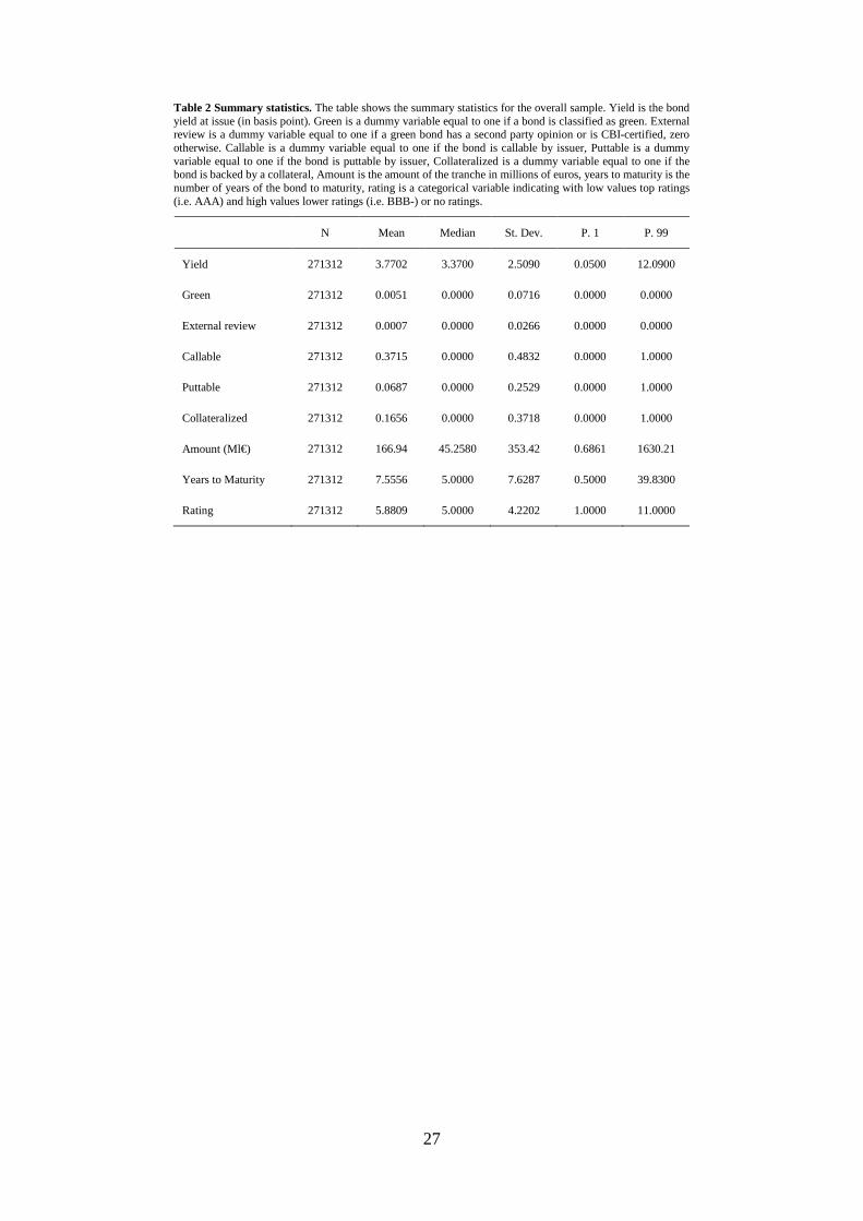
27

Table 2 Summary statistics. The table shows the summary statistics for the overall sample. Yield is the bond yield at issue (in basis point). Green is a dummy variable equal to one if a bond is classified as green. External review is a dummy variable equal to one if a green bond has a second party opinion or is CBI-certified, zero otherwise. Callable is a dummy variable equal to one if the bond is callable by issuer, Puttable is a dummy variable equal to one if the bond is puttable by issuer, Collateralized is a dummy variable equal to one if the bond is backed by a collateral, Amount is the amount of the tranche in millions of euros, years to maturity is the number of years of the bond to maturity, rating is a categorical variable indicating with low values top ratings (i.e. AAA) and high values lower ratings (i.e. BBB-) or no ratings.

N Mean Median St. Dev. P. 1 P. 99

Yield 271312 3.7702 3.3700 2.5090 0.0500 12.0900

Green 271312 0.0051 0.0000 0.0716 0.0000 0.0000

External review 271312 0.0007 0.0000 0.0266 0.0000 0.0000

Callable 271312 0.3715 0.0000 0.4832 0.0000 1.0000

Puttable 271312 0.0687 0.0000 0.2529 0.0000 1.0000

Collateralized 271312 0.1656 0.0000 0.3718 0.0000 1.0000

Amount (Ml€) 271312 166.94 45.2580 353.42 0.6861 1630.21

Years to Maturity 271312 7.5556 5.0000 7.6287 0.5000 39.8300

Rating 271312 5.8809 5.0000 4.2202 1.0000 11.0000

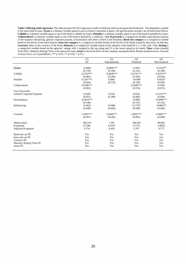
28

Table 3 Offering yield regression. The table presents the OLS regression results of offering yield on the green bond indicator. The dependent variable is the bond yield at issue. Green is a dummy variable equal to one if a bond is classified as green. All specifications include a set of bond fixed effects. Callable is a dummy variable equal to one if the bond is callable by issuer, Puttable is a dummy variable equal to one if the bond is puttable by issuer, Collateralized is a dummy variable equal to one if the bond is backed by a collateral, , Use of proceeds is a categorical variable capturing the purpose of the issuance refinancing, general corporate purpose, securitization and others (which is the baseline), Bond size category is a categorical variable based on the decile of the bond amount, Issue size category is a categorical variable based on the decile of the bonds issued by that issuer on that day, Currency refers to the currency of the bond, Maturity is a categorical variable based on the maturity of the bond (0-5 y, 5-10y, and >10y), Rating is a categorical variable based on the agencies’ ratings with 1 assigned to the top rating and 11 to the worst rating (or no rated), Time is time (month) fixed effect, Maturity×Rating×Time is the interaction term, Issuer is the fixed effect for the company issuing the bond. Robust standard errors, clustered at issuer level, are in parentheses. *** p<0.01, ** p<0.05, * p<0.1.

(1) (2) (3) (4) All Supranational Financial Non-financial Green -0.2866 -0.8046*** 0.1001 -0.2156** (0.178) (0.149) (0.312) (0.108) Callable 0.2518*** -0.4640*** 0.2741*** 0.2253*** (0.083) (0.106) (0.100) (0.034) Puttable 0.1207*** 0.0861 -0.0548 0.0542* (0.044) (0.219) (0.158) (0.030) Collateralized 0.3298*** 0.2949*** 0.0766 (0.065) (0.074) (0.075) Use of proceeds General Corporate Purposes 0.0294 0.2241 0.0353 0.1233*** (0.051) (0.288) (0.085) (0.044) Securitisation -0.3633*** -0.0801 -0.6990*** (0.140) (0.147) (0.142) Refinancing -0.0435 0.0386 0.1770* -0.0892** (0.048) (0.664) (0.099) (0.044) Constant 3.5876*** 5.0464*** 2.9697*** 4.5865*** (0.057) (0.282) (0.092) (0.044) Observations 266,724 7,391 168,594 89,902 R-squared 0.7296 0.4767 0.7176 0.8056 Adjusted R-squared 0.714 0.436 0.707 0.775 Bond size cat FE Yes Yes Yes Yes Issue size cat FE Yes Yes Yes Yes Currency FE Yes Yes Yes Yes Maturity×Rating×Time FE Yes Yes Yes Yes Issuer FE Yes Yes Yes Yes

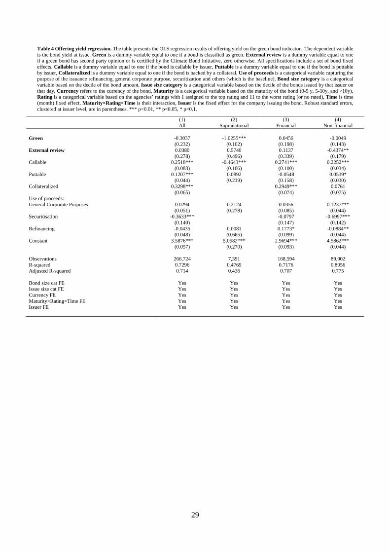
29

Table 4 Offering yield regression. The table presents the OLS regression results of offering yield on the green bond indicator. The dependent variable is the bond yield at issue. Green is a dummy variable equal to one if a bond is classified as green. External review is a dummy variable equal to one if a green bond has second party opinion or is certified by the Climate Bond Initiative, zero otherwise. All specifications include a set of bond fixed effects. Callable is a dummy variable equal to one if the bond is callable by issuer, Puttable is a dummy variable equal to one if the bond is puttable by issuer, Collateralized is a dummy variable equal to one if the bond is backed by a collateral, Use of proceeds is a categorical variable capturing the purpose of the issuance refinancing, general corporate purpose, securitization and others (which is the baseline), Bond size category is a categorical variable based on the decile of the bond amount, Issue size category is a categorical variable based on the decile of the bonds issued by that issuer on that day, Currency refers to the currency of the bond, Maturity is a categorical variable based on the maturity of the bond (0-5 y, 5-10y, and >10y), Rating is a categorical variable based on the agencies’ ratings with 1 assigned to the top rating and 11 to the worst rating (or no rated), Time is time (month) fixed effect, Maturity×Rating×Time is their interaction, Issuer is the fixed effect for the company issuing the bond. Robust standard errors, clustered at issuer level, are in parentheses. *** p<0.01, ** p<0.05, * p<0.1.

(1) (2) (3) (4) All Supranational Financial Non-financial Green -0.3037 -1.0255*** 0.0456 -0.0049 (0.232) (0.102) (0.198) (0.143) External review 0.0380 0.5740 0.1137 -0.4374** (0.278) (0.496) (0.339) (0.179) Callable 0.2518*** -0.4643*** 0.2741*** 0.2252*** (0.083) (0.106) (0.100) (0.034) Puttable 0.1207*** 0.0892 -0.0548 0.0539* (0.044) (0.219) (0.158) (0.030) Collateralized 0.3298*** 0.2949*** 0.0761 (0.065) (0.074) (0.075) Use of proceeds: General Corporate Purposes 0.0294 0.2124 0.0356 0.1237*** (0.051) (0.278) (0.085) (0.044) Securitisation -0.3633*** -0.0797 -0.6997*** (0.140) (0.147) (0.142) Refinancing -0.0435 0.0081 0.1773* -0.0884** (0.048) (0.665) (0.099) (0.044) Constant 3.5876*** 5.0582*** 2.9694*** 4.5862*** (0.057) (0.270) (0.093) (0.044) Observations 266,724 7,391 168,594 89,902 R-squared 0.7296 0.4769 0.7176 0.8056 Adjusted R-squared 0.714 0.436 0.707 0.775 Bond size cat FE Yes Yes Yes Yes Issue size cat FE Yes Yes Yes Yes Currency FE Yes Yes Yes Yes Maturity×Rating×Time FE Yes Yes Yes Yes Issuer FE Yes Yes Yes Yes

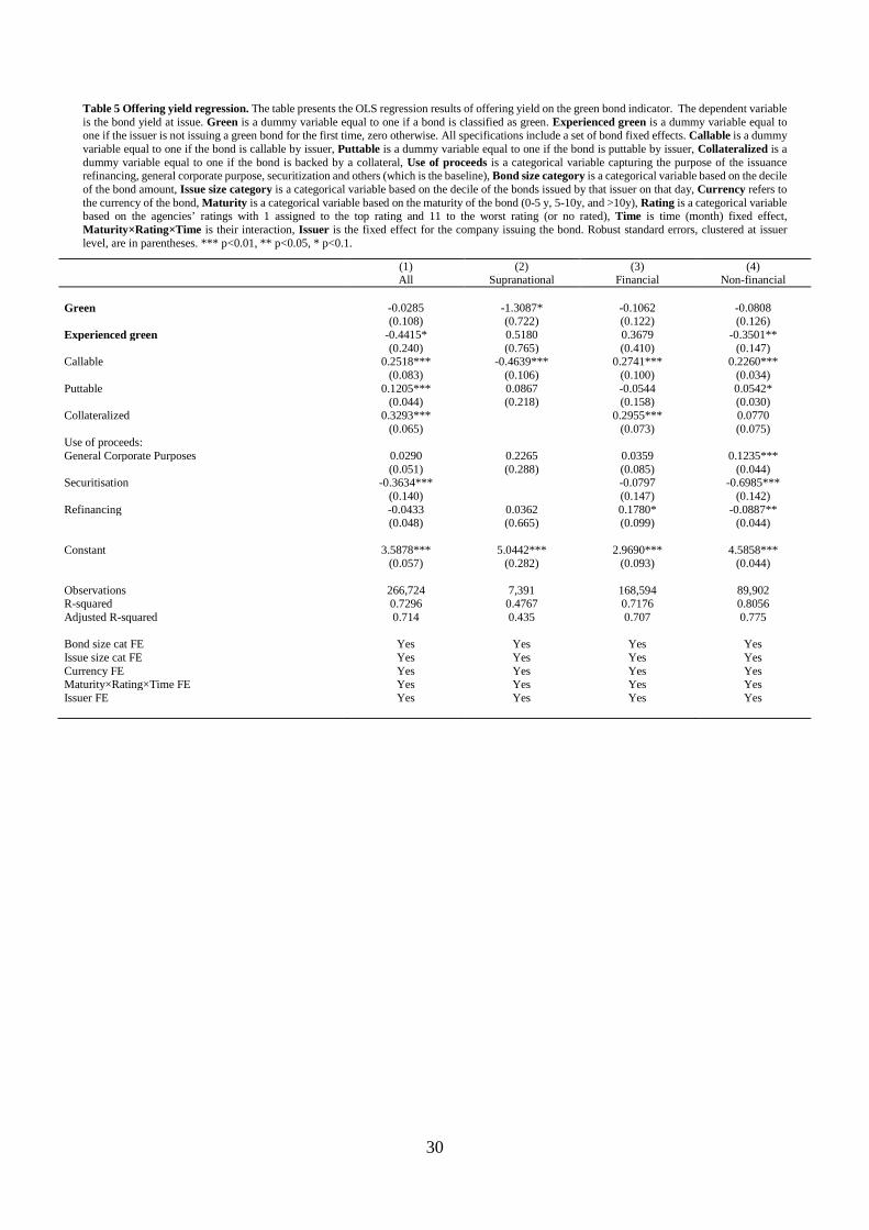
30

Table 5 Offering yield regression. The table presents the OLS regression results of offering yield on the green bond indicator. The dependent variable is the bond yield at issue. Green is a dummy variable equal to one if a bond is classified as green. Experienced green is a dummy variable equal to one if the issuer is not issuing a green bond for the first time, zero otherwise. All specifications include a set of bond fixed effects. Callable is a dummy variable equal to one if the bond is callable by issuer, Puttable is a dummy variable equal to one if the bond is puttable by issuer, Collateralized is a dummy variable equal to one if the bond is backed by a collateral, Use of proceeds is a categorical variable capturing the purpose of the issuance refinancing, general corporate purpose, securitization and others (which is the baseline), Bond size category is a categorical variable based on the decile of the bond amount, Issue size category is a categorical variable based on the decile of the bonds issued by that issuer on that day, Currency refers to the currency of the bond, Maturity is a categorical variable based on the maturity of the bond (0-5 y, 5-10y, and >10y), Rating is a categorical variable based on the agencies’ ratings with 1 assigned to the top rating and 11 to the worst rating (or no rated), Time is time (month) fixed effect, Maturity×Rating×Time is their interaction, Issuer is the fixed effect for the company issuing the bond. Robust standard errors, clustered at issuer level, are in parentheses. *** p<0.01, ** p<0.05, * p<0.1.

(1) (2) (3) (4) All Supranational Financial Non-financial Green -0.0285 -1.3087* -0.1062 -0.0808 (0.108) (0.722) (0.122) (0.126) Experienced green -0.4415* 0.5180 0.3679 -0.3501** (0.240) (0.765) (0.410) (0.147) Callable 0.2518*** -0.4639*** 0.2741*** 0.2260*** (0.083) (0.106) (0.100) (0.034) Puttable 0.1205*** 0.0867 -0.0544 0.0542* (0.044) (0.218) (0.158) (0.030) Collateralized 0.3293*** 0.2955*** 0.0770 (0.065) (0.073) (0.075) Use of proceeds: General Corporate Purposes 0.0290 0.2265 0.0359 0.1235*** (0.051) (0.288) (0.085) (0.044) Securitisation -0.3634*** -0.0797 -0.6985*** (0.140) (0.147) (0.142) Refinancing -0.0433 0.0362 0.1780* -0.0887** (0.048) (0.665) (0.099) (0.044) Constant 3.5878*** 5.0442*** 2.9690*** 4.5858*** (0.057) (0.282) (0.093) (0.044) Observations 266,724 7,391 168,594 89,902 R-squared 0.7296 0.4767 0.7176 0.8056 Adjusted R-squared 0.714 0.435 0.707 0.775 Bond size cat FE Yes Yes Yes Yes Issue size cat FE Yes Yes Yes Yes Currency FE Yes Yes Yes Yes Maturity×Rating×Time FE Yes Yes Yes Yes Issuer FE Yes Yes Yes Yes

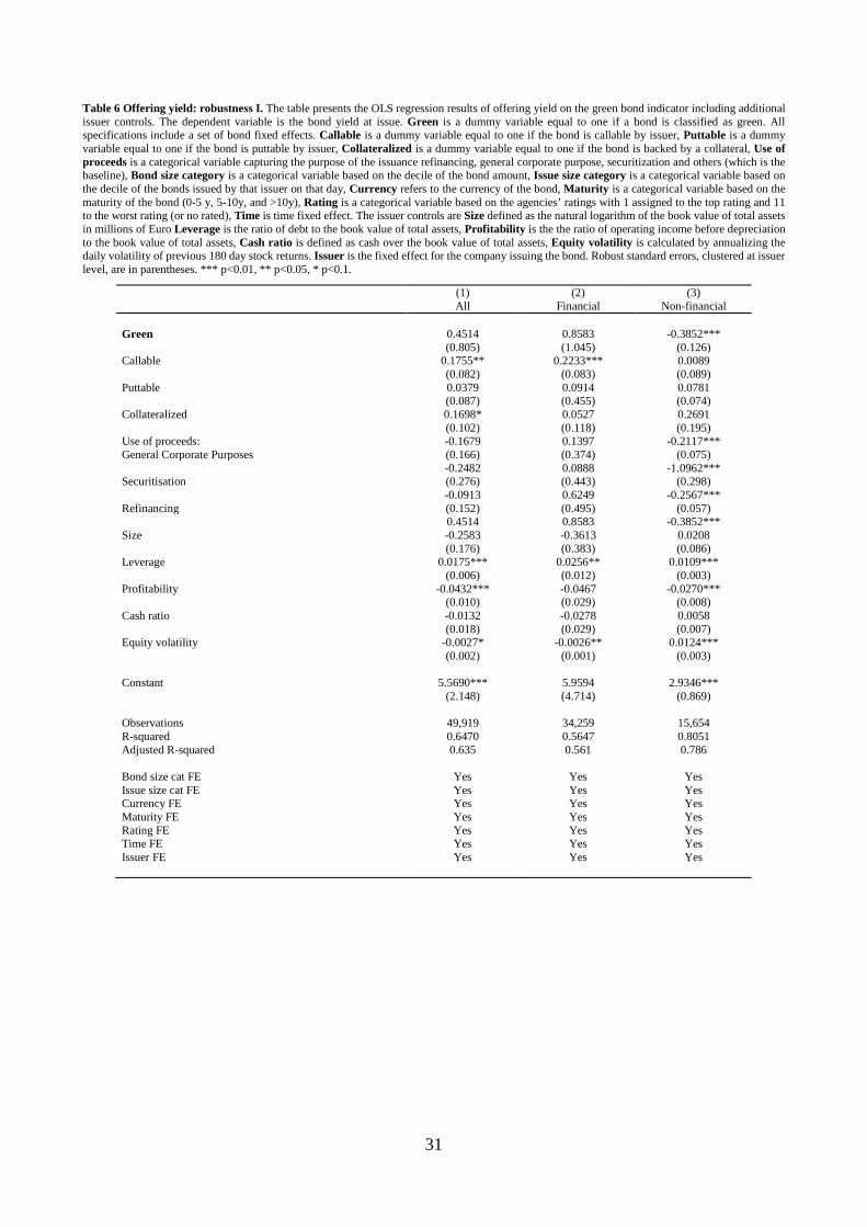
31

Table 6 Offering yield: robustness I. The table presents the OLS regression results of offering yield on the green bond indicator including additional issuer controls. The dependent variable is the bond yield at issue. Green is a dummy variable equal to one if a bond is classified as green. All specifications include a set of bond fixed effects. Callable is a dummy variable equal to one if the bond is callable by issuer, Puttable is a dummy variable equal to one if the bond is puttable by issuer, Collateralized is a dummy variable equal to one if the bond is backed by a collateral, Use of proceeds is a categorical variable capturing the purpose of the issuance refinancing, general corporate purpose, securitization and others (which is the baseline), Bond size category is a categorical variable based on the decile of the bond amount, Issue size category is a categorical variable based on the decile of the bonds issued by that issuer on that day, Currency refers to the currency of the bond, Maturity is a categorical variable based on the maturity of the bond (0-5 y, 5-10y, and >10y), Rating is a categorical variable based on the agencies’ ratings with 1 assigned to the top rating and 11 to the worst rating (or no rated), Time is time fixed effect. The issuer controls are Size defined as the natural logarithm of the book value of total assets in millions of Euro Leverage is the ratio of debt to the book value of total assets, Profitability is the the ratio of operating income before depreciation to the book value of total assets, Cash ratio is defined as cash over the book value of total assets, Equity volatility is calculated by annualizing the daily volatility of previous 180 day stock returns. Issuer is the fixed effect for the company issuing the bond. Robust standard errors, clustered at issuer level, are in parentheses. *** p<0.01, ** p<0.05, * p<0.1.

(1) (2) (3) All Financial Non-financial Green 0.4514 0.8583 -0.3852*** (0.805) (1.045) (0.126) Callable 0.1755** 0.2233*** 0.0089 (0.082) (0.083) (0.089) Puttable 0.0379 0.0914 0.0781 (0.087) (0.455) (0.074) Collateralized 0.1698* 0.0527 0.2691 (0.102) (0.118) (0.195) Use of proceeds: -0.1679 0.1397 -0.2117*** General Corporate Purposes (0.166) (0.374) (0.075) -0.2482 0.0888 -1.0962*** Securitisation (0.276) (0.443) (0.298) -0.0913 0.6249 -0.2567*** Refinancing (0.152) (0.495) (0.057) 0.4514 0.8583 -0.3852*** Size -0.2583 -0.3613 0.0208 (0.176) (0.383) (0.086) Leverage 0.0175*** 0.0256** 0.0109*** (0.006) (0.012) (0.003) Profitability -0.0432*** -0.0467 -0.0270*** (0.010) (0.029) (0.008) Cash ratio -0.0132 -0.0278 0.0058 (0.018) (0.029) (0.007) Equity volatility -0.0027* -0.0026** 0.0124*** (0.002) (0.001) (0.003) Constant 5.5690*** 5.9594 2.9346*** (2.148) (4.714) (0.869) Observations 49,919 34,259 15,654 R-squared 0.6470 0.5647 0.8051 Adjusted R-squared 0.635 0.561 0.786 Bond size cat FE Yes Yes Yes Issue size cat FE Yes Yes Yes Currency FE Yes Yes Yes Maturity FE Yes Yes Yes Rating FE Yes Yes Yes Time FE Yes Yes Yes Issuer FE Yes Yes Yes

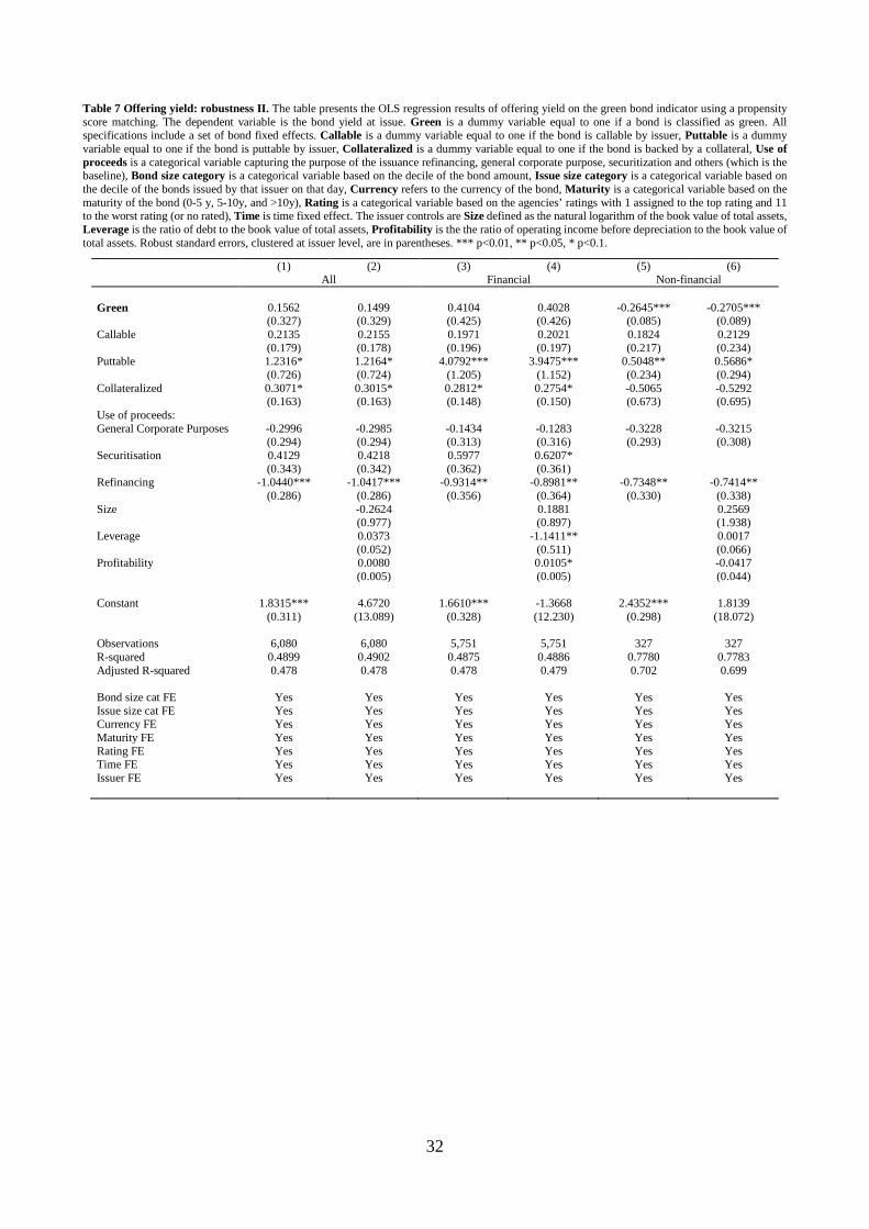
32

Table 7 Offering yield: robustness II. The table presents the OLS regression results of offering yield on the green bond indicator using a propensity score matching. The dependent variable is the bond yield at issue. Green is a dummy variable equal to one if a bond is classified as green. All specifications include a set of bond fixed effects. Callable is a dummy variable equal to one if the bond is callable by issuer, Puttable is a dummy variable equal to one if the bond is puttable by issuer, Collateralized is a dummy variable equal to one if the bond is backed by a collateral, Use of proceeds is a categorical variable capturing the purpose of the issuance refinancing, general corporate purpose, securitization and others (which is the baseline), Bond size category is a categorical variable based on the decile of the bond amount, Issue size category is a categorical variable based on the decile of the bonds issued by that issuer on that day, Currency refers to the currency of the bond, Maturity is a categorical variable based on the maturity of the bond (0-5 y, 5-10y, and >10y), Rating is a categorical variable based on the agencies’ ratings with 1 assigned to the top rating and 11 to the worst rating (or no rated), Time is time fixed effect. The issuer controls are Size defined as the natural logarithm of the book value of total assets, Leverage is the ratio of debt to the book value of total assets, Profitability is the the ratio of operating income before depreciation to the book value of total assets. Robust standard errors, clustered at issuer level, are in parentheses. *** p<0.01, ** p<0.05, * p<0.1.

(1) (2) (3) (4) (5) (6) All Financial Non-financial Green 0.1562 0.1499 0.4104 0.4028 -0.2645*** -0.2705*** (0.327) (0.329) (0.425) (0.426) (0.085) (0.089) Callable 0.2135 0.2155 0.1971 0.2021 0.1824 0.2129 (0.179) (0.178) (0.196) (0.197) (0.217) (0.234) Puttable 1.2316* 1.2164* 4.0792*** 3.9475*** 0.5048** 0.5686* (0.726) (0.724) (1.205) (1.152) (0.234) (0.294) Collateralized 0.3071* 0.3015* 0.2812* 0.2754* -0.5065 -0.5292 (0.163) (0.163) (0.148) (0.150) (0.673) (0.695) Use of proceeds: General Corporate Purposes -0.2996 -0.2985 -0.1434 -0.1283 -0.3228 -0.3215 (0.294) (0.294) (0.313) (0.316) (0.293) (0.308) Securitisation 0.4129 0.4218 0.5977 0.6207* (0.343) (0.342) (0.362) (0.361) Refinancing -1.0440*** -1.0417*** -0.9314** -0.8981** -0.7348** -0.7414** (0.286) (0.286) (0.356) (0.364) (0.330) (0.338) Size -0.2624 0.1881 0.2569 (0.977) (0.897) (1.938) Leverage 0.0373 -1.1411** 0.0017 (0.052) (0.511) (0.066) Profitability 0.0080 0.0105* -0.0417 (0.005) (0.005) (0.044) Constant 1.8315*** 4.6720 1.6610*** -1.3668 2.4352*** 1.8139 (0.311) (13.089) (0.328) (12.230) (0.298) (18.072) Observations 6,080 6,080 5,751 5,751 327 327 R-squared 0.4899 0.4902 0.4875 0.4886 0.7780 0.7783 Adjusted R-squared 0.478 0.478 0.478 0.479 0.702 0.699 Bond size cat FE Yes Yes Yes Yes Yes Yes Issue size cat FE Yes Yes Yes Yes Yes Yes Currency FE Yes Yes Yes Yes Yes Yes Maturity FE Yes Yes Yes Yes Yes Yes Rating FE Yes Yes Yes Yes Yes Yes Time FE Yes Yes Yes Yes Yes Yes Issuer FE Yes Yes Yes Yes Yes Yes

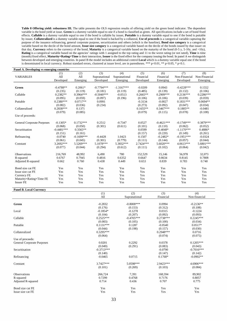
33

Table 8 Offering yield: robustness III. The table presents the OLS regression results of offering yield on the green bond indicator. The dependent variable is the bond yield at issue. Green is a dummy variable equal to one if a bond is classified as green. All specifications include a set of bond fixed effects. Callable is a dummy variable equal to one if the bond is callable by issuer, Puttable is a dummy variable equal to one if the bond is puttable by issuer, Collateralized is a dummy variable equal to one if the bond is backed by a collateral, Use of proceeds is a categorical variable capturing the purpose of the issuance refinancing, general corporate purpose, securitization and others (which is the baseline), Bond size category is a categorical variable based on the decile of the bond amount, Issue size category is a categorical variable based on the decile of the bonds issued by that issuer on that day, Currency refers to the currency of the bond, Maturity is a categorical variable based on the maturity of the bond (0-5 y, 5-10y, and >10y), Rating is a categorical variable based on the agencies’ ratings with 1 assigned to the top rating and 11 to the worst rating (or not rated), Time is time (month) fixed effect, Maturity×Rating×Time is their interaction, Issuer is the fixed effect for the company issuing the bond. In panel A we distinguish between developed and emerging countries. In panel B the model includes an additional control Local which is a dummy variable equal one if the bond is denominated in local currency. Robust standard errors, clustered at issuer level, are in parentheses. *** p<0.01, ** p<0.05, * p<0.1.

Panel A. Developing vs emerging countries (1) (2) (3) (4) (5) (6) (7) (8) VARIABLES All

Developed All

Emerging Supranational

Developed Supranational

Emerging Financial

Developed Financial Emerging

Non-Financial Developed

Non-Financial Emerging

Green -0.4788** 0.2061* -0.7794*** -1.3167*** -0.0209 0.0943 -0.4228*** 0.1552 (0.235) (0.119) (0.181) (0.119) (0.485) (0.139) (0.132) (0.106) Callable 0.2382** 0.3964*** -0.5040*** -0.0513 0.2665** 0.2909*** 0.2136*** 0.2286*** (0.095) (0.059) (0.097) (0.196) (0.106) (0.106) (0.039) (0.059) Puttable 0.2380*** 0.0717** 0.0991 -0.3134 -0.0027 0.1831*** 0.0694** (0.082) (0.036) (0.234) (0.273) (0.092) (0.047) (0.034) Collateralized 0.2838*** 0.1371 0.1655** 0.3467*** 0.1805** -0.0481 (0.079) (0.085) (0.079) (0.115) (0.078) (0.108) Use of proceeds:

General Corporate Purposes -0.1305* 0.1732*** 0.2512 -0.7347 0.0527 -0.4621*** -0.1749*** 0.3879*** (0.068) (0.050) (0.301) (0.611) (0.101) (0.110) (0.062) (0.052) Securitisation -0.4481*** 0.3565** 0.0599 -0.4048* -1.1170*** 0.4886* (0.151) (0.161) (0.157) (0.220) (0.149) (0.261) Refinancing -0.0740 -0.1699*** -0.4428 1.0423 0.1507 -0.2482* -0.1951*** -0.0324 (0.061) (0.045) (0.301) (0.779) (0.111) (0.144) (0.057) (0.044) Constant 3.2692*** 5.5269*** 5.1078*** 5.3832*** 2.7424*** 5.6020*** 4.0613*** 5.6801*** (0.077) (0.044) (0.294) (0.612) (0.111) (0.102) (0.064) (0.042) Observations 216,769 48,992 6,490 780 152,529 15,146 56,978 32,073 R-squared 0.6767 0.7945 0.4816 0.6352 0.6647 0.8634 0.8145 0.7808 Adjusted R-squared 0.662 0.760 0.438 0.449 0.653 0.839 0.783 0.740 Bond size cat FE Yes Yes Yes Yes Yes Yes Yes Yes Issue size cat FE Yes Yes Yes Yes Yes Yes Yes Yes Currency FE Yes Yes Yes Yes Yes Yes Yes Yes Maturity×Rating×Time FE Yes Yes Yes Yes Yes Yes Yes Yes Issuer FE Yes Yes Yes Yes Yes Yes Yes Yes

Panel B. Local Currency (1) (2) (3) (4) All Supranational Financial Non-financial Green -0.2832 -0.8008*** 0.0994 -0.2136** (0.176) (0.153) (0.312) (0.108) Local -0.1854* -0.1278 0.0315 -0.1224 (0.104) (0.207) (0.092) (0.093) Callable 0.2525*** -0.4705*** 0.2738*** 0.2245*** (0.083) (0.105) (0.100) (0.034) Puttable 0.1131*** 0.1287 -0.0540 0.0517* (0.044) (0.198) (0.157) (0.030) Collateralized 0.3295*** 0.2948*** 0.0716 (0.064) (0.074) (0.075) Use of proceeds: General Corporate Purposes 0.0201 0.2292 0.0378 0.1205*** (0.049) (0.291) (0.083) (0.043) Securitisation -0.3713*** -0.0790 -0.7016*** (0.140) (0.147) (0.142) Refinancing -0.0465 0.0715 0.1768* -0.0902** Constant 3.7427*** 5.0598*** 2.9423*** 4.6906*** (0.101) (0.269) (0.103) (0.084) Observations 266,724 7,391 168,594 89,902 R-squared 0.7299 0.4768 0.7176 0.8057 Adjusted R-squared 0.714 0.436 0.707 0.775 Bond size cat FE Yes Yes Yes Yes Issue size cat FE Yes Yes Yes Yes

34

Currency FE Yes Yes Yes Yes Maturity×Rating×Time FE Yes Yes Yes Yes Issuer FE Yes Yes Yes Yes

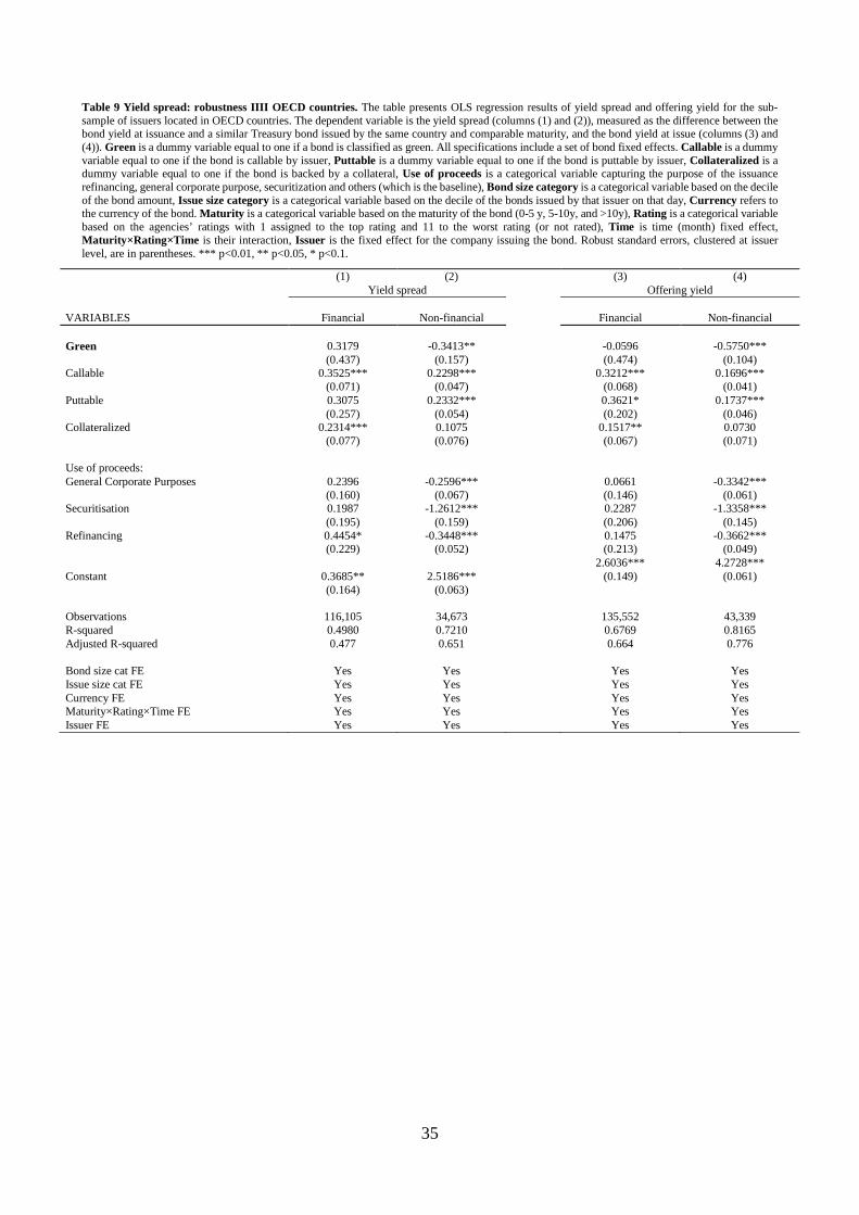
35

Table 9 Yield spread: robustness IIII OECD countries. The table presents OLS regression results of yield spread and offering yield for the sub-sample of issuers located in OECD countries. The dependent variable is the yield spread (columns (1) and (2)), measured as the difference between the bond yield at issuance and a similar Treasury bond issued by the same country and comparable maturity, and the bond yield at issue (columns (3) and (4)). Green is a dummy variable equal to one if a bond is classified as green. All specifications include a set of bond fixed effects. Callable is a dummy variable equal to one if the bond is callable by issuer, Puttable is a dummy variable equal to one if the bond is puttable by issuer, Collateralized is a dummy variable equal to one if the bond is backed by a collateral, Use of proceeds is a categorical variable capturing the purpose of the issuance refinancing, general corporate purpose, securitization and others (which is the baseline), Bond size category is a categorical variable based on the decile of the bond amount, Issue size category is a categorical variable based on the decile of the bonds issued by that issuer on that day, Currency refers to the currency of the bond. Maturity is a categorical variable based on the maturity of the bond (0-5 y, 5-10y, and >10y), Rating is a categorical variable based on the agencies’ ratings with 1 assigned to the top rating and 11 to the worst rating (or not rated), Time is time (month) fixed effect, Maturity×Rating×Time is their interaction, Issuer is the fixed effect for the company issuing the bond. Robust standard errors, clustered at issuer level, are in parentheses. *** p<0.01, ** p<0.05, * p<0.1.

(1) (2) (3) (4) Yield spread Offering yield VARIABLES Financial Non-financial Financial Non-financial Green 0.3179 -0.3413** -0.0596 -0.5750*** (0.437) (0.157) (0.474) (0.104) Callable 0.3525*** 0.2298*** 0.3212*** 0.1696*** (0.071) (0.047) (0.068) (0.041) Puttable 0.3075 0.2332*** 0.3621* 0.1737*** (0.257) (0.054) (0.202) (0.046) Collateralized 0.2314*** 0.1075 0.1517** 0.0730 (0.077) (0.076) (0.067) (0.071) Use of proceeds: General Corporate Purposes 0.2396 -0.2596*** 0.0661 -0.3342*** (0.160) (0.067) (0.146) (0.061) Securitisation 0.1987 -1.2612*** 0.2287 -1.3358*** (0.195) (0.159) (0.206) (0.145) Refinancing 0.4454* -0.3448*** 0.1475 -0.3662*** (0.229) (0.052) (0.213) (0.049) 2.6036*** 4.2728*** Constant 0.3685** 2.5186*** (0.149) (0.061) (0.164) (0.063) Observations 116,105 34,673 135,552 43,339 R-squared 0.4980 0.7210 0.6769 0.8165 Adjusted R-squared 0.477 0.651 0.664 0.776 Bond size cat FE Yes Yes Yes Yes Issue size cat FE Yes Yes Yes Yes Currency FE Yes Yes Yes Yes Maturity×Rating×Time FE Yes Yes Yes Yes Issuer FE Yes Yes Yes Yes

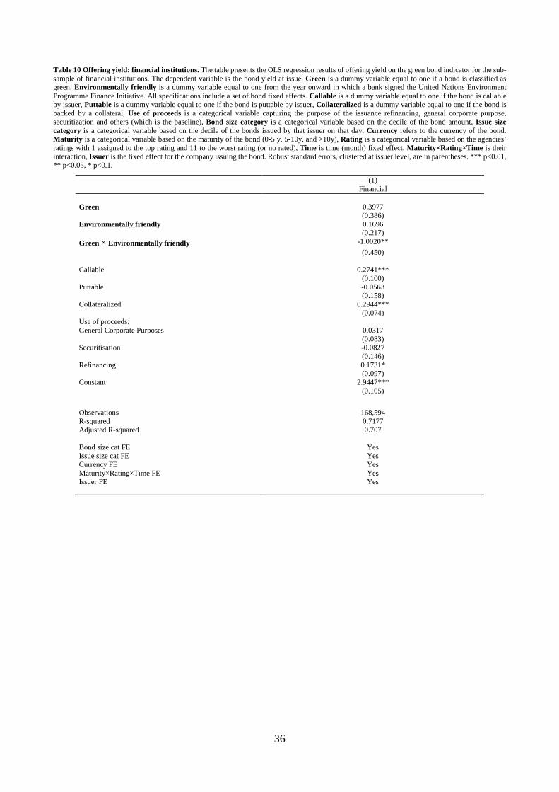
36

Table 10 Offering yield: financial institutions. The table presents the OLS regression results of offering yield on the green bond indicator for the sub-sample of financial institutions. The dependent variable is the bond yield at issue. Green is a dummy variable equal to one if a bond is classified as green. Environmentally friendly is a dummy variable equal to one from the year onward in which a bank signed the United Nations Environment Programme Finance Initiative. All specifications include a set of bond fixed effects. Callable is a dummy variable equal to one if the bond is callable by issuer, Puttable is a dummy variable equal to one if the bond is puttable by issuer, Collateralized is a dummy variable equal to one if the bond is backed by a collateral, Use of proceeds is a categorical variable capturing the purpose of the issuance refinancing, general corporate purpose, securitization and others (which is the baseline), Bond size category is a categorical variable based on the decile of the bond amount, Issue size category is a categorical variable based on the decile of the bonds issued by that issuer on that day, Currency refers to the currency of the bond. Maturity is a categorical variable based on the maturity of the bond (0-5 y, 5-10y, and >10y), Rating is a categorical variable based on the agencies’ ratings with 1 assigned to the top rating and 11 to the worst rating (or no rated), Time is time (month) fixed effect, Maturity×Rating×Time is their interaction, Issuer is the fixed effect for the company issuing the bond. Robust standard errors, clustered at issuer level, are in parentheses. *** p<0.01, ** p<0.05, * p<0.1.

(1) Financial Green 0.3977 (0.386) Environmentally friendly 0.1696 (0.217) Green × Environmentally friendly -1.0020** (0.450) Callable 0.2741*** (0.100) Puttable -0.0563 (0.158) Collateralized 0.2944*** (0.074) Use of proceeds: General Corporate Purposes 0.0317 (0.083) Securitisation -0.0827 (0.146) Refinancing 0.1731* (0.097) Constant 2.9447*** (0.105) Observations 168,594 R-squared 0.7177 Adjusted R-squared 0.707 Bond size cat FE Yes Issue size cat FE Yes Currency FE Yes Maturity×Rating×Time FE Yes Issuer FE Yes

37

Table 11. Green issuer and lending decisions: summary statistics. The table shows the summary statistics for the sample of bank lending. The unit of observation is the bank-country-industry-year level, based on the sample of all completed syndicated loans from 2007 to 2018 granted to industry-country (jc) for which bank b served as lead arranger in year t. The sample is limited to bank-industry-country (bjc) with non-zero loans in at least two years. Amount is the logarithm of the total amount granted to industry-country (jc) for which bank b served as lead arranger in year t, plus one. Average amount is the logarithm of the average amount granted to industry-country (jc) for which bank b served as lead arranger in year t, plus one. Any loan is a dummy variable which takes value one if any loans were granted to industry-country jc by bank b in period t, zero otherwise. Green issuer is a dummy variable which takes value one from the time t the bank b has issued a green bond onwards, zero otherwise. Emission intensities is the ratio between greenhouse gasses and the value added for a specific industry j in country c in period t. Emission intensities 2 is the ratio between greenhouse gasses and the output for a specific industry j in country c in period t. The unit of measure is kilograms per Euro.

Variable N Mean Median St. Dev. P. 1 P. 99 Amount 69180 3.3092 0.0000 4.4904 0.0000 11.8679 Average amount 69180 3.0225 0.0000 4.1017 0.0000 10.9739 Any loan 69180 0.3589 0.0000 0.4797 0.0000 1.0000 Green issuer 69180 0.1504 0.0000 0.3575 0.0000 1.0000 Emission intensities

65455 0.6381 0.0498 1.5643 0.0000 7.6062

Emission intensities 2

65380 0.2074 0.0231 0.4905 0.0000 2.6389

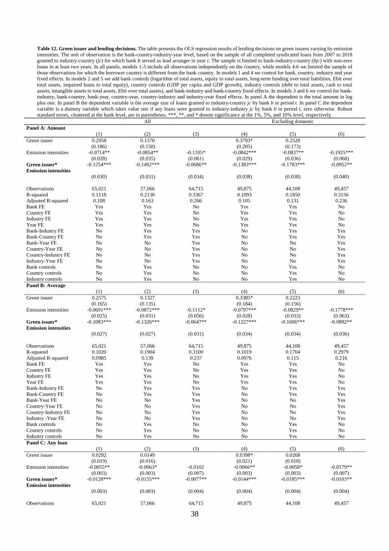
38

Table 12. Green issuer and lending decisions. The table presents the OLS regression results of lending decisions on green issuers varying by emission intensities. The unit of observation is the bank-country-industry-year level, based on the sample of all completed syndicated loans from 2007 to 2018 granted to industry-country (jc) for which bank b served as lead arranger in year t. The sample is limited to bank-industry-country (bjc) with non-zero loans in at least two years. In all panels, models 1-3 include all observations independently on the country, while models 4-6 we limited the sample of those observations for which the borrower country is different from the bank country. In models 1 and 4 we control for bank, country, industry and year fixed effects. In models 2 and 5 we add bank controls (logarithm of total assets, equity to total assets, long-term funding over total liabilities, Ebit over total assets, impaired loans to total equity), country controls (GDP per capita and GDP growth), industry controls (debt to total assets, cash to total assets, intangible assets to total assets, Ebit over total assets), and bank-industry and bank-country fixed effects. In models 3 and 6 we control for bank-industry, bank-country, bank-year, country-year, country-industry and industry-year fixed effects. In panel A the dependent is the total amount in log plus one. In panel B the dependent variable is the average size of loans granted to industry-country jc by bank b in period t. In panel C the dependent variable is a dummy variable which takes value one if any loans were granted to industry-industry jc by bank b in period t, zero otherwise. Robust standard errors, clustered at the bank level, are in parentheses. ***, **, and * denote significance at the 1%, 5%, and 10% level, respectively.

All Excluding domestic Panel A: Amount (1) (2) (3) (4) (5) (6) Green issuer 0.2958 0.1570 0.3793* 0.2528 (0.186) (0.150) (0.205) (0.173) Emission intensities -0.0714** -0.0854** -0.1105* -0.0842*** -0.0837** -0.1925*** (0.028) (0.035) (0.061) (0.029) (0.036) (0.068) Green issuer* Emission intensities

-0.1254*** -0.1492*** -0.0686** -0.1383*** -0.1783*** -0.0952**

(0.030) (0.031) (0.034) (0.038) (0.038) (0.040) Observations 65,021 57,066 64,715 49,875 44,108 49,457 R-squared 0.1118 0.2130 0.3367 0.1093 0.1850 0.3156 Adjusted R-squared 0.108 0.163 0.266 0.105 0.131 0.236 Bank FE Yes Yes No Yes Yes No Country FE Yes Yes No Yes Yes No Industry FE Yes Yes No Yes Yes No Year FE Yes Yes No Yes Yes No Bank-Industry FE No Yes Yes No Yes Yes Bank-Country FE No Yes Yes No Yes Yes Bank-Year FE No No Yes No No Yes Country-Year FE No No Yes No No Yes Country-Industry FE No No Yes No No Yes Industry-Year FE No No Yes No No Yes Bank controls No Yes No No Yes No Country controls No Yes No No Yes No Industry controls No Yes No No Yes No Panel B: Average (1) (2) (3) (4) (5) (6) Green issuer 0.2575 0.1327 0.3385* 0.2223 (0.165) (0.135) (0.184) (0.156) Emission intensities -0.0691*** -0.0872*** -0.1112* -0.0797*** -0.0829** -0.1778*** (0.025) (0.031) (0.056) (0.028) (0.033) (0.063) Green issuer* Emission intensities

-0.1083*** -0.1326*** -0.0647** -0.1227*** -0.1606*** -0.0892**

(0.027) (0.027) (0.031) (0.034) (0.034) (0.036) Observations 65,021 57,066 64,715 49,875 44,108 49,457 R-squared 0.1020 0.1904 0.3100 0.1019 0.1704 0.2979 Adjusted R-squared 0.0985 0.139 0.237 0.0976 0.115 0.216 Bank FE Yes Yes No Yes Yes No Country FE Yes Yes No Yes Yes No Industry FE Yes Yes No Yes Yes No Year FE Yes Yes No Yes Yes No Bank-Industry FE No Yes Yes No Yes Yes Bank-Country FE No Yes Yes No Yes Yes Bank-Year FE No No Yes No No Yes Country-Year FE No No Yes No No Yes Country-Industry FE No No Yes No No Yes Industry -Year FE No No Yes No No Yes Bank controls No Yes No No Yes No Country controls No Yes No No Yes No Industry controls No Yes No No Yes No Panel C: Any loan (1) (2) (3) (4) (5) (6) Green issuer 0.0292 0.0149 0.0398* 0.0268 (0.019) (0.016) (0.021) (0.018) Emission intensities -0.0055** -0.0063* -0.0102 -0.0066** -0.0058* -0.0179** (0.003) (0.003) (0.007) (0.003) (0.003) (0.007) Green issuer* Emission intensities

-0.0128*** -0.0155*** -0.0077** -0.0144*** -0.0185*** -0.0103**

(0.003) (0.003) (0.004) (0.004) (0.004) (0.004) Observations 65,021 57,066 64,715 49,875 44,108 49,457

39

R-squared 0.0982 0.1902 0.3059 0.0966 0.1647 0.2898 Adjusted R-squared 0.0946 0.138 0.232 0.0923 0.109 0.207 Bank FE Yes Yes No Yes Yes No Country FE Yes Yes No Yes Yes No Industry FE Yes Yes No Yes Yes No Year FE Yes Yes No Yes Yes No Bank-Industry FE No Yes Yes No Yes Yes Bank-Country FE No Yes Yes No Yes Yes Bank-Year FE No No Yes No No Yes Country-Year FE No No Yes No No Yes Country-Industry FE No No Yes No No Yes Industry -Year FE No No Yes No No Yes Bank controls No Yes No No Yes No Country controls No Yes No No Yes No Industry controls No Yes No No Yes No

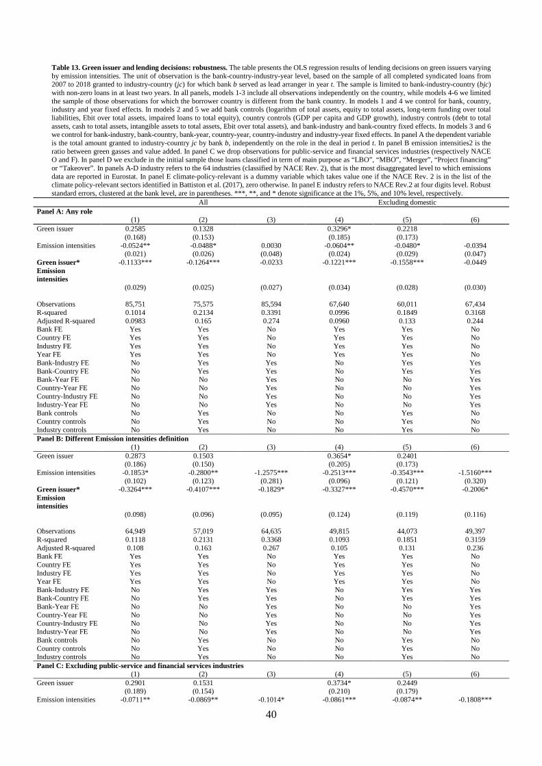
40

Table 13. Green issuer and lending decisions: robustness. The table presents the OLS regression results of lending decisions on green issuers varying by emission intensities. The unit of observation is the bank-country-industry-year level, based on the sample of all completed syndicated loans from 2007 to 2018 granted to industry-country (jc) for which bank b served as lead arranger in year t. The sample is limited to bank-industry-country (bjc) with non-zero loans in at least two years. In all panels, models 1-3 include all observations independently on the country, while models 4-6 we limited the sample of those observations for which the borrower country is different from the bank country. In models 1 and 4 we control for bank, country, industry and year fixed effects. In models 2 and 5 we add bank controls (logarithm of total assets, equity to total assets, long-term funding over total liabilities, Ebit over total assets, impaired loans to total equity), country controls (GDP per capita and GDP growth), industry controls (debt to total assets, cash to total assets, intangible assets to total assets, Ebit over total assets), and bank-industry and bank-country fixed effects. In models 3 and 6 we control for bank-industry, bank-country, bank-year, country-year, country-industry and industry-year fixed effects. In panel A the dependent variable is the total amount granted to industry-country jc by bank b, independently on the role in the deal in period t. In panel B emission intensities2 is the ratio between green gasses and value added. In panel C we drop observations for public-service and financial services industries (respectively NACE O and F). In panel D we exclude in the initial sample those loans classified in term of main purpose as “LBO”, “MBO”, “Merger”, “Project financing” or “Takeover”. In panels A-D industry refers to the 64 industries (classified by NACE Rev. 2), that is the most disaggregated level to which emissions data are reported in Eurostat. In panel E climate-policy-relevant is a dummy variable which takes value one if the NACE Rev. 2 is in the list of the climate policy-relevant sectors identified in Battiston et al. (2017), zero otherwise. In panel E industry refers to NACE Rev.2 at four digits level. Robust standard errors, clustered at the bank level, are in parentheses. ***, **, and * denote significance at the 1%, 5%, and 10% level, respectively.

All Excluding domestic Panel A: Any role (1) (2) (3) (4) (5) (6) Green issuer 0.2585 0.1328 0.3296* 0.2218 (0.168) (0.153) (0.185) (0.173) Emission intensities -0.0524** -0.0488* 0.0030 -0.0604** -0.0480* -0.0394 (0.021) (0.026) (0.048) (0.024) (0.029) (0.047) Green issuer* Emission intensities

-0.1133*** -0.1264*** -0.0233 -0.1221*** -0.1558*** -0.0449

(0.029) (0.025) (0.027) (0.034) (0.028) (0.030) Observations 85,751 75,575 85,594 67,640 60,011 67,434 R-squared 0.1014 0.2134 0.3391 0.0996 0.1849 0.3168 Adjusted R-squared 0.0983 0.165 0.274 0.0960 0.133 0.244 Bank FE Yes Yes No Yes Yes No Country FE Yes Yes No Yes Yes No Industry FE Yes Yes No Yes Yes No Year FE Yes Yes No Yes Yes No Bank-Industry FE No Yes Yes No Yes Yes Bank-Country FE No Yes Yes No Yes Yes Bank-Year FE No No Yes No No Yes Country-Year FE No No Yes No No Yes Country-Industry FE No No Yes No No Yes Industry-Year FE No No Yes No No Yes Bank controls No Yes No No Yes No Country controls No Yes No No Yes No Industry controls No Yes No No Yes No Panel B: Different Emission intensities definition (1) (2) (3) (4) (5) (6) Green issuer 0.2873 0.1503 0.3654* 0.2401 (0.186) (0.150) (0.205) (0.173) Emission intensities -0.1853* -0.2800** -1.2575*** -0.2513*** -0.3543*** -1.5160*** (0.102) (0.123) (0.281) (0.096) (0.121) (0.320) Green issuer* Emission intensities

-0.3264*** -0.4107*** -0.1829* -0.3327*** -0.4570*** -0.2006*

(0.098) (0.096) (0.095) (0.124) (0.119) (0.116) Observations 64,949 57,019 64,635 49,815 44,073 49,397 R-squared 0.1118 0.2131 0.3368 0.1093 0.1851 0.3159 Adjusted R-squared 0.108 0.163 0.267 0.105 0.131 0.236 Bank FE Yes Yes No Yes Yes No Country FE Yes Yes No Yes Yes No Industry FE Yes Yes No Yes Yes No Year FE Yes Yes No Yes Yes No Bank-Industry FE No Yes Yes No Yes Yes Bank-Country FE No Yes Yes No Yes Yes Bank-Year FE No No Yes No No Yes Country-Year FE No No Yes No No Yes Country-Industry FE No No Yes No No Yes Industry-Year FE No No Yes No No Yes Bank controls No Yes No No Yes No Country controls No Yes No No Yes No Industry controls No Yes No No Yes No Panel C: Excluding public-service and financial services industries (1) (2) (3) (4) (5) (6) Green issuer 0.2901 0.1531 0.3734* 0.2449 (0.189) (0.154) (0.210) (0.179) Emission intensities -0.0711** -0.0869** -0.1014* -0.0861*** -0.0874** -0.1808***

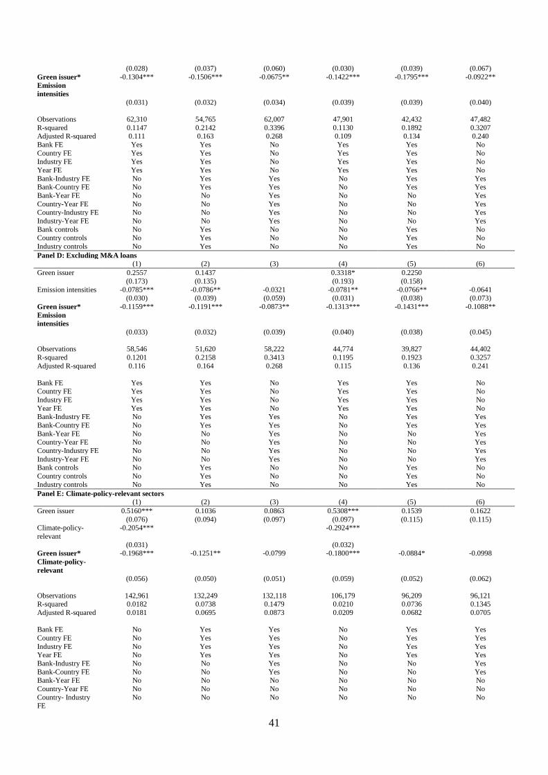
41

(0.028) (0.037) (0.060) (0.030) (0.039) (0.067) Green issuer* Emission intensities

-0.1304*** -0.1506*** -0.0675** -0.1422*** -0.1795*** -0.0922**

(0.031) (0.032) (0.034) (0.039) (0.039) (0.040) Observations 62,310 54,765 62,007 47,901 42,432 47,482 R-squared 0.1147 0.2142 0.3396 0.1130 0.1892 0.3207 Adjusted R-squared 0.111 0.163 0.268 0.109 0.134 0.240 Bank FE Yes Yes No Yes Yes No Country FE Yes Yes No Yes Yes No Industry FE Yes Yes No Yes Yes No Year FE Yes Yes No Yes Yes No Bank-Industry FE No Yes Yes No Yes Yes Bank-Country FE No Yes Yes No Yes Yes Bank-Year FE No No Yes No No Yes Country-Year FE No No Yes No No Yes Country-Industry FE No No Yes No No Yes Industry-Year FE No No Yes No No Yes Bank controls No Yes No No Yes No Country controls No Yes No No Yes No Industry controls No Yes No No Yes No Panel D: Excluding M&A loans (1) (2) (3) (4) (5) (6) Green issuer 0.2557 0.1437 0.3318* 0.2250 (0.173) (0.135) (0.193) (0.158) Emission intensities -0.0785*** -0.0786** -0.0321 -0.0781** -0.0766** -0.0641 (0.030) (0.039) (0.059) (0.031) (0.038) (0.073) Green issuer* Emission intensities

-0.1159*** -0.1191*** -0.0873** -0.1313*** -0.1431*** -0.1088**

(0.033) (0.032) (0.039) (0.040) (0.038) (0.045) Observations 58,546 51,620 58,222 44,774 39,827 44,402 R-squared 0.1201 0.2158 0.3413 0.1195 0.1923 0.3257 Adjusted R-squared 0.116 0.164 0.268 0.115 0.136 0.241 Bank FE Yes Yes No Yes Yes No Country FE Yes Yes No Yes Yes No Industry FE Yes Yes No Yes Yes No Year FE Yes Yes No Yes Yes No Bank-Industry FE No Yes Yes No Yes Yes Bank-Country FE No Yes Yes No Yes Yes Bank-Year FE No No Yes No No Yes Country-Year FE No No Yes No No Yes Country-Industry FE No No Yes No No Yes Industry-Year FE No No Yes No No Yes Bank controls No Yes No No Yes No Country controls No Yes No No Yes No Industry controls No Yes No No Yes No Panel E: Climate-policy-relevant sectors (1) (2) (3) (4) (5) (6) Green issuer 0.5160*** 0.1036 0.0863 0.5308*** 0.1539 0.1622 (0.076) (0.094) (0.097) (0.097) (0.115) (0.115) Climate-policy-relevant

-0.2054*** -0.2924***

(0.031) (0.032) Green issuer* Climate-policy-relevant

-0.1968*** -0.1251** -0.0799 -0.1800*** -0.0884* -0.0998

(0.056) (0.050) (0.051) (0.059) (0.052) (0.062) Observations 142,961 132,249 132,118 106,179 96,209 96,121 R-squared 0.0182 0.0738 0.1479 0.0210 0.0736 0.1345 Adjusted R-squared 0.0181 0.0695 0.0873 0.0209 0.0682 0.0705 Bank FE No Yes Yes No Yes Yes Country FE No Yes Yes No Yes Yes Industry FE No Yes Yes No Yes Yes Year FE No Yes Yes No Yes Yes Bank-Industry FE No No Yes No No Yes Bank-Country FE No No Yes No No Yes Bank-Year FE No No No No No No Country-Year FE No No No No No No Country- Industry FE

No No No No No No

42

Industry -Year FE No No No No No No Bank controls Yes Yes Yes Yes Yes Yes Country controls Yes Yes Yes Yes Yes Yes NACE controls Yes Yes Yes Yes Yes Yes

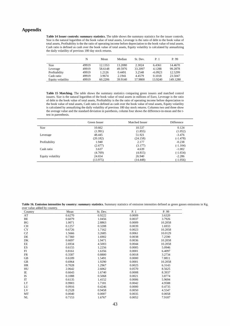
43

Appendix Table 14 Issuer controls: summary statistics. The table shows the summary statistics for the issuer controls. Size is the natural logarithm of the book value of total assets, Leverage is the ratio of debt to the book value of total assets, Profitability is the the ratio of operating income before depreciation to the book value of total assets, Cash ratio is defined as cash over the book value of total assets, Equity volatility is calculated by annualizing the daily volatility of previous 180 day stock returns.

N Mean Median St. Dev. P. 1 P. 99

Size 49919 12.1353 13.2080 2.3024 6.4361 14.4670 Leverage 49919 58.6148 49.5976 33.2097 4.1288 99.2878 Profitability 49919 1.2126 0.4491 3.2548 -6.0923 12.5299 Cash ratio 49919 3.9674 2.1941 4.4579 0.1018 23.5047 Equity volatility 49919 60.2206 39.9140 57.9800 13.9240 149.1280

Table 15 Matching. The table shows the summary statistics comparing green issuers and matched control issuers. Size is the natural logarithm of the book value of total assets in millions of Euro, Leverage is the ratio of debt to the book value of total assets, Profitability is the the ratio of operating income before depreciation to the book value of total assets, Cash ratio is defined as cash over the book value of total assets, Equity volatility is calculated by annualizing the daily volatility of previous 180 day stock returns. Columns two and three show the average value and the standard deviation in parethesis, column four shows the difference-in-mean and the t-test in parenthesis.

Green Issuer Matched Issuer Difference

Size 10.662 10.537 0.124 (1.991) (1.855) (1.052) Leverage 48.445 51.921 -3.476 (20.182) (24.158) (-1.478) Profitability 1.940 2.177 -0.238 (2.677) (3.177) (-1.104) Cash ratio 3.637 4.639 -1.002 (4.769) (4.815) (-1.654) Equity volatility 24.654 26.940 -2.286 (13.975) (14.448) (-1.056)

Table 16. Emission intensities by country: summary statistics. Summary statistics of emission intensities defined as green gasses emissions in Kg. over value added by country.

Country Mean St. Dev. P. 1 P. 99 AT 0.6270 0.9222 0.0009 3.6320 BE 0.6079 1.0456 0.0037 3.7926 BG 1.0071 2.8863 0.0009 10.2058 CH 0.1257 0.3208 0.0039 1.6933 CY 0.6726 1.7162 0.0023 10.2058 CZ 1.5666 3.2685 0.0061 10.0129 DE 0.7360 1.6902 0.0038 7.2590 DK 0.6697 1.9471 0.0036 10.2058 EE 2.6934 4.5003 0.0044 10.2058 ES 0.6155 1.2256 0.0005 5.0946 FI 0.8161 1.6356 0.0001 6.4097 FR 0.3587 0.8800 0.0018 3.2734 GB 0.6189 1.5491 0.0000 7.8811 GR 0.6964 1.9290 0.0001 10.2058 HR 0.7028 1.2967 0.0025 6.3143 HU 2.0642 2.6062 0.0570 8.5625 IE 0.6643 1.6740 0.0008 8.3937 IS 0.1088 0.5068 0.0021 3.8774 IT 0.6135 1.4152 0.0006 5.9694 LT 0.9903 1.7181 0.0042 4.9588 LU 0.0916 0.4246 0.0000 0.4735 LV 0.2528 0.9458 0.0050 4.5547 MT 0.0040 0.0007 0.0035 0.0058 NL 0.7153 1.6767 0.0052 7.9187

44

NO 0.4591 0.8339 0.0000 3.2592 PL 2.0241 3.1831 0.0180 10.2058 PT 1.2786 2.0778 0.0007 7.5096 RO 1.9389 2.6136 0.0155 10.2058 RS 0.0592 0.0712 0.0209 0.4516 SE 0.4153 1.0227 0.0018 5.7084 SI 0.3807 1.3905 0.0000 7.7436 SK 1.9644 2.8958 0.0166 10.2058 TR 1.2407 2.9056 0.0000 10.2058

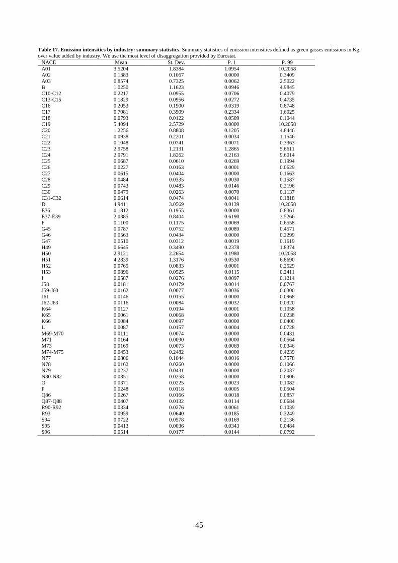
45

Table 17. Emission intensities by industry: summary statistics. Summary statistics of emission intensities defined as green gasses emissions in Kg. over value added by industry. We use the most level of disaggregation provided by Eurostat.

NACE Mean St. Dev. P. 1 P. 99 A01 3.5204 1.8384 1.0954 10.2058 A02 0.1383 0.1067 0.0000 0.3409 A03 0.8574 0.7325 0.0062 2.5022 B 1.0250 1.1623 0.0946 4.9845 C10-C12 0.2217 0.0955 0.0706 0.4079 C13-C15 0.1829 0.0956 0.0272 0.4735 C16 0.2053 0.1900 0.0319 0.8748 C17 0.7081 0.3909 0.2334 1.6025 C18 0.0793 0.0122 0.0509 0.1044 C19 5.4094 2.5729 0.0000 10.2058 C20 1.2256 0.8808 0.1205 4.8446 C21 0.0938 0.2201 0.0034 1.1546 C22 0.1048 0.0741 0.0071 0.3363 C23 2.9758 1.2131 1.2865 5.6611 C24 2.9791 1.8262 0.2163 9.6014 C25 0.0687 0.0610 0.0269 0.1994 C26 0.0227 0.0163 0.0001 0.0629 C27 0.0615 0.0404 0.0000 0.1663 C28 0.0484 0.0335 0.0030 0.1587 C29 0.0743 0.0483 0.0146 0.2196 C30 0.0479 0.0263 0.0070 0.1137 C31-C32 0.0614 0.0474 0.0041 0.1818 D 4.9411 3.0569 0.0139 10.2058 E36 0.1812 0.1955 0.0000 0.8361 E37-E39 2.0385 0.8404 0.6190 3.5266 F 0.1100 0.1175 0.0069 0.6558 G45 0.0787 0.0752 0.0089 0.4571 G46 0.0563 0.0434 0.0000 0.2299 G47 0.0510 0.0312 0.0019 0.1619 H49 0.6645 0.3490 0.2378 1.8374 H50 2.9121 2.2654 0.1980 10.2058 H51 4.2839 1.3176 0.0530 6.8690 H52 0.0765 0.0833 0.0001 0.2529 H53 0.0896 0.0525 0.0115 0.2411 I 0.0587 0.0276 0.0097 0.1214 J58 0.0181 0.0179 0.0014 0.0767 J59-J60 0.0162 0.0077 0.0036 0.0300 J61 0.0146 0.0155 0.0000 0.0968 J62-J63 0.0116 0.0084 0.0032 0.0320 K64 0.0127 0.0194 0.0001 0.1058 K65 0.0061 0.0068 0.0000 0.0238 K66 0.0084 0.0097 0.0000 0.0400 L 0.0087 0.0157 0.0004 0.0728 M69-M70 0.0111 0.0074 0.0000 0.0431 M71 0.0164 0.0090 0.0000 0.0564 M73 0.0169 0.0073 0.0069 0.0346 M74-M75 0.0453 0.2482 0.0000 0.4239 N77 0.0806 0.1044 0.0016 0.7578 N78 0.0162 0.0260 0.0000 0.1066 N79 0.0237 0.0431 0.0000 0.2037 N80-N82 0.0351 0.0258 0.0000 0.0906 O 0.0371 0.0225 0.0023 0.1082 P 0.0248 0.0118 0.0005 0.0504 Q86 0.0267 0.0166 0.0018 0.0857 Q87-Q88 0.0407 0.0132 0.0114 0.0684 R90-R92 0.0334 0.0276 0.0061 0.1039 R93 0.0959 0.0640 0.0185 0.3249 S94 0.0722 0.0578 0.0169 0.2136 S95 0.0413 0.0036 0.0343 0.0484 S96 0.0514 0.0177 0.0144 0.0792

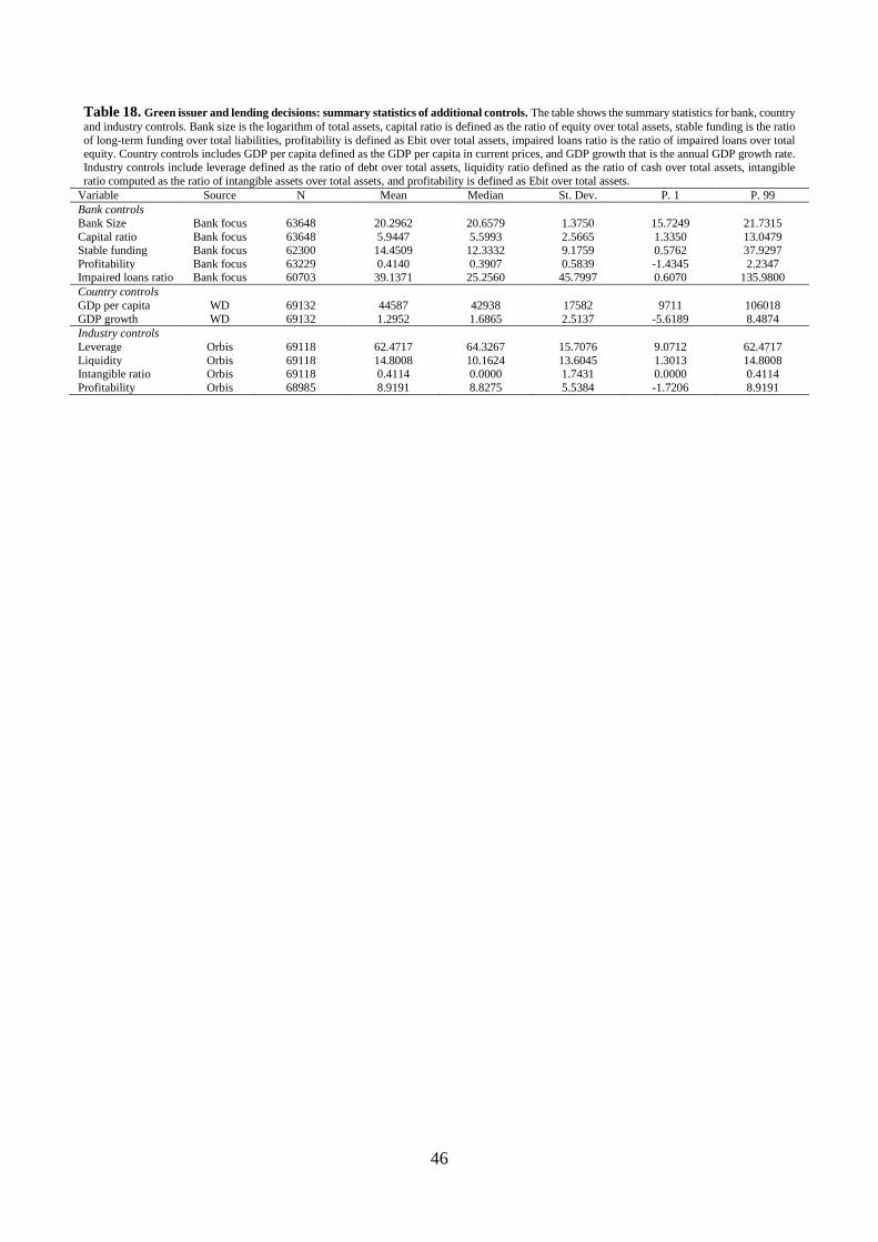
46

Table 18. Green issuer and lending decisions: summary statistics of additional controls. The table shows the summary statistics for bank, country and industry controls. Bank size is the logarithm of total assets, capital ratio is defined as the ratio of equity over total assets, stable funding is the ratio of long-term funding over total liabilities, profitability is defined as Ebit over total assets, impaired loans ratio is the ratio of impaired loans over total equity. Country controls includes GDP per capita defined as the GDP per capita in current prices, and GDP growth that is the annual GDP growth rate. Industry controls include leverage defined as the ratio of debt over total assets, liquidity ratio defined as the ratio of cash over total assets, intangible ratio computed as the ratio of intangible assets over total assets, and profitability is defined as Ebit over total assets.

Variable Source N Mean Median St. Dev. P. 1 P. 99 Bank controls Bank Size Bank focus 63648 20.2962 20.6579 1.3750 15.7249 21.7315 Capital ratio Bank focus 63648 5.9447 5.5993 2.5665 1.3350 13.0479 Stable funding Bank focus 62300 14.4509 12.3332 9.1759 0.5762 37.9297 Profitability Bank focus 63229 0.4140 0.3907 0.5839 -1.4345 2.2347 Impaired loans ratio Bank focus 60703 39.1371 25.2560 45.7997 0.6070 135.9800 Country controls GDp per capita WD 69132 44587 42938 17582 9711 106018 GDP growth WD 69132 1.2952 1.6865 2.5137 -5.6189 8.4874 Industry controls Leverage Orbis 69118 62.4717 64.3267 15.7076 9.0712 62.4717 Liquidity Orbis 69118 14.8008 10.1624 13.6045 1.3013 14.8008 Intangible ratio Orbis 69118 0.4114 0.0000 1.7431 0.0000 0.4114 Profitability Orbis 68985 8.9191 8.8275 5.5384 -1.7206 8.9191