Embed Size (px)
Citation preview
This is the accepted version. For the published version, see the July 2008 issue of Sociology of Education.
Are “Failing” Schools Really Failing?Removing the Influence of Non-School Factors from Measures of School Quality
Douglas B. Downey*Paul T. von Hippel
Melanie Hughes
The Ohio State University
*Direct all correspondence to Douglas B. Downey, Department of Sociology, 300 Bricker Hall, 190 N. Oval Mall, Columbus, Ohio 43210, ([email protected]). Phone (614) 292-1352, Fax (614) 292-6681. This project was funded by grants from NICHD (R03 HD043917-01), the Spencer Foundation (Downey and von Hippel), the John Glenn Institute (Downey), and the Ohio State P-12 Project (Downey). The contributions of the first two authors are equal. We appreciate the comments of Beckett Broh, Donna Bobbitt-Zeher, Benjamin Gibbs, and Brian Powell.
Failing Schools? 2
Abstract
To many it is obvious which schools are failing—those whose students perform poorly
on achievement tests. But evaluating schools on achievement mixes the effect of school factors
(e.g., good teachers) with the effect of non-school factors (e.g., homes and neighborhoods) in
unknown ways. As a result, achievement-based evaluation likely underestimates the
effectiveness of schools serving disadvantaged populations. We discuss school-evaluation
methods that more effectively separate school effects from non-school effects. Specifically, we
consider evaluating schools using 12-month (calendar-year) learning rates, 9-month (school-
year) learning rates, and a provocative new measure, “impact,” which is the difference between
the school-year learning rate and the summer learning rate. Using data from the Early Childhood
Longitudinal Study of 1998-99, we show that learning- or impact-based evaluation methods
substantially change our conclusions about which schools are failing. In particular, among
schools with failing (bottom-quintile) achievement levels, less than half are failing with respect
to learning or impact. In addition, schools serving disadvantaged students are much more likely
to have low achievement levels than they are to have low levels of learning or impact. We
discuss the implications of these findings for market-based education reform.
This is the accepted version. For the published version, see the July 2008 issue of Sociology of Education.
Are “Failing” Schools Really Failing?Removing the Influence of Non-School Factors from Measures of School Quality
Market-based reforms pervade current education policy discussions in the United States. The
potential for markets to promote efficiency, long recognized in the private sector, represents an
attractive mechanism by which to improve the quality of public education, especially among urban
schools serving poor students, where inefficiency is suspected (Chubb and Moe 1990; Walberg and
Bast 2003). The rapid growth of charter schools (Renzulli and Roscigno 2005) and the emphasis on
accountability in the No Child Left Behind Act (NCLB) are prompted by the belief that when parents
have information about school quality, accompanied by a choice about where to send their children,
competitive pressure will prompt administrators and teachers to improve schools by working harder
and smarter.
Of course, critical to market success is the need for consumers (i.e., parents) to have good
information about service quality (i.e., schools) because market efficiency is undermined if
information is unavailable or inaccurate (Ladd 2002). Toward this end, NCLB requires states to make
public their evaluations of schools, addressing the need for information on quality to be easily
accessible.
But does the available information provide valid measures of school quality? Are the schools
designated as “failing,” under current criteria, really the least effective schools? Under most current
evaluation systems, “failing” schools are defined as schools with low average achievement scores.
The basis for this definition of school failure is the assumption that student achievement is a direct
measure of school quality. But we know that this assumption is wrong. As the Coleman Report and
other research highlighted decades ago, achievement scores have more to do with family influences
than with school quality (Coleman et. al 1966; Jencks et al., 1972). It follows that a valid system of
Failing Schools? 4
school evaluation must separate school effects from non-school effects on children’s achievement and
learning.
Since the Coleman Report, sociologists’ contributions to school evaluation have been less
visible, with current education legislation dominated by ideas from economics and, to a lesser extent,
psychology. In this paper, we show how ideas and methods from sociology can make important
contributions in the effort to separate school effects from non-school effects. Specifically, we
consider evaluating schools using 12-month (calendar-year) learning rates, 9-month (school-year)
learning rates, and a provocative new measure, “impact,” which is the difference between the school-
year learning rate and the summer learning rate. The impact measure is unique in that its theoretical
and methodological roots are in sociology.
One might expect that the method of evaluation would have little effect on which schools
appear to be ineffective. After all, schools identified as “failing” under achievement-based methods
do look like the worst schools. They not only have low test scores, but they also tend to have high
teacher turnover, low resource levels, and poor morale (Thenstrom and Thernstrom 2003). Yet we
will show that if we evaluate schools using learning or impact—i.e., if we try to isolate the effect of
school from non-school factors on students’ learning—our ideas about “failing” schools change in
important ways. Among schools that are failing under an achievement-based criterion, less than half
are failing under criteria based on learning or impact. In addition, roughly one-fifth of schools with
satisfactory achievement scores turn up among the poorest performers with respect to learning or
impact.
These patterns suggest that raw achievement levels cannot be considered an accurate measure
of school effectiveness; accurately gauging school performance requires new approaches. As long as
school quality is evaluated using measures based on achievement, accountability-based school reform
will have limited utility for helping schools to improve.
Failing Schools? 5
THREE MEASURES OF SCHOOL EFFECTIVNESS
In this section, we review the most widely used method for evaluating schools—achievement—and
contrast it with less-often-used methods based on learning or gains. We discuss the practice of using
student characteristics to “adjust” achievement or gains, and we highlight the problems inherent in
making such adjustments. We then introduce a third evaluation measure that we call impact—which
measures the degree to which a schools’ students learn faster when they are in school (during the
academic year) than when they are not (during summer vacation).
Achievement
Because success in the economy, and in life, typically requires a certain level of academic skill, the
No Child Left Behind legislation generally holds schools accountable for their students’ level of
achievement or proficiency. At present, NCLB allows each state to define proficiency and set its own
proficiency bar (Ryan 2004), but the legislation provides guidelines about how proficiency is to be
measured. For example, NCLB requires all states to test children in math and reading annually
between grades 3-8 and at least once between grades 10-12, while in science states are only required
to test students three times between grades 3 and 12. As one example of how states have responded,
the Department of Education in Ohio complies with NCLB by using an achievement-bar standard for
Ohio schools based on twenty test scores spanning different grades and subjects, as well as two
indicators (attendance and graduation rates) that are not based on test scores.
In some modest and temporary ways, the NCLB legislation acknowledges that schools serve
children of varying non-school environments, and that these non-school influences may have some
effect on children’s achievement levels. For example, schools with low test scores are not expected to
clear the state’s proficiency bar immediately; they can satisfy state requirements by making “adequate
yearly progress” toward the desired level for the first several years. (The definition of “adequate
Failing Schools? 6
yearly progress” varies by state.1) In this way, the legislation recognizes that schools serving poor
children will need some time to catch up and reach the proficiency standards expected of all schools.
By 2013-14, however, all schools are expected to reach the standard. More importantly, the schools
that “need improvement” are being identified on the basis of their achievement scores.
The main problem with evaluating schools this way is that achievement tests do not
adequately separate school and non-school effects on children’s learning. It is likely that a schools’
test scores are a function not just of school practices (e.g., good teaching and efficient administration)
but also of non-school characteristics (e.g., involved parenting and high-resource neighborhoods). So
it is not clear the extent to which schools with high test scores are necessarily “good” schools, and
schools with low test scores are necessarily “failing.” Students are not randomly assigned to schools,
and there is substantial variation in the kinds of students who attend different schools. When
attempting to evaluate schools, therefore, the challenge is to measure the value that schools add
independently from the widely varying non-school factors that also influence achievement.
Sociologists have documented extensively the importance of the home environment to
children’s development, along with the substantial variation in children’s home experiences. As one
example of how much home environments vary in cognitive stimulation, Hart and Risley (1995)
observed that among children six months to three years old, welfare children had 616 words per hour
directed to them compared to 1,251 for working-class and 2,153 for professional-family children.
Given such varying exposure to language, it is not surprising that large skill gaps can be observed
among children at the beginning of kindergarten. For example, eighteen percent of children entering
kindergarten in the U.S. in the fall of 1998 did not know that print reads left to right, did not know
where to go when a line of print ends, and did not know where the story ends in a book (West,
1 In Ohio, adequately yearly progress typically means reducing the gap between a school’s or district’s baseline performance (average of 1999-2000, 2000-01, 2001-02 years) and the proficiency
Failing Schools? 7
Denton, and Germino-Hausken 2000). At the other end of the spectrum, a small percentage of
children beginning kindergarten could already read words in context (West, Denton, and Germino-
Hausken 2000).
Widely varying skills among children, of course, would not be so problematic for our goal of
measuring school effectiveness if children’s initial achievement levels were randomly distributed
across schools, but even on the first day of kindergarten, achievement levels vary substantially from
one school to another(Downey, von Hippel, and Broh 2004; Lee and Burkam 2002; Reardon 2003).
At the start of kindergarten, 21 percent of the variation in reading test scores and 25 percent of the
variation in math test scores lies between rather than within schools (Downey et. al. 2004). In other
words, substantial differences between school achievement levels are observable even before schools
have a chance to matter. Obviously these variations are not a consequence of differences in school
quality but represent the fact that schools serve different kinds of students.
Although children’s achievement is clearly influenced by both school and non-school factors,
achievement-based methods of evaluating schools assume that only schools matter. As a result, the
burden of improvement ends up being disproportionately placed on schools serving children from
poor non-school environments, even though it is not clear that these schools are any less effective than
schools serving children from advantaged environments. Although some schools serving
disadvantaged populations may actually be poor-quality schools, without separating school from non-
school effects it is difficult to make this evaluation with confidence.
These criticisms of achievement-based measures of school effectiveness are, by now, well-
established in the social science community (c.f., Teddlie and Reynolds 1999; Scheerens and Bosker
1997).
bar by 10 percentage points per year between 2003-04 and 2013-14.
Failing Schools? 8
Learning
One way to measure school effectiveness that begins to address differences in non-school factors is to
gauge how much students learn in a year, rather than where they end up on an achievement scale. The
advantage of an approach based on learning is that schools are not rewarded or penalized for the
achievement level of their students at the beginning of the year. Under a learning-based evaluation
system, schools serving children with initially high achievement would be challenged to raise
performance even further, while schools serving disadvantaged students could be deemed “effective”
if its students made substantial progress from an initially low achievement level, even if their final
achievement level was still somewhat low.
One example of a learning-based evaluation system is the Tennessee Value Added Assessment
System (TVAAS), implemented by the state of Tennessee in 1992 to assess its teachers and schools.
Under TVAAS, students are measured each year, and data are compiled into a longitudinally merged
database linking individual outcomes to teachers, schools, and districts (Chatterji 2002). Estimates of
average student achievement progress are calculated for each school and teacher, and the model then
determines a school’s performance on the basis of estimated gain scores of a school relative to the
norm group’s gain on a given grade-level test (Kupermintz 2002).
Tennessee is not the only state with learning-based accountability. North and South Carolina
have implemented systems similar to TVAAS, as has the city of Dallas (Ladd and Walsh 2002).
Since NCLB was first passed, politicians and lawmakers have also come to recognize the advantages
of learning-based measures. Indeed, in 2005, the U.S. Secretary of Education announced that states
could collect data on children’s learning or achievement growth (along with the current information
on raw achievement) to eventually be used for accountability purposes. Several states have since
Failing Schools? 9
gained approval from the Department of Education to pilot “growth model” accountability systems.2
Outside of the policymaking arena, education scholars have also produced a wide range of useful
indictors of students’ learning (for overviews see Teddlie and Reynolds 1999; Scheerens and Bosker
1997).
Our extension of this useful work is to note an important limitation to learning-based measures
of school effectiveness—the amount learned in a year is still not entirely under schools’ control. The
simplest way to see this is to recognize that, even during the academic year, children spend most of
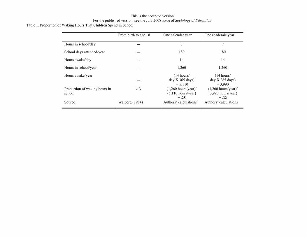
their time outside of the school environment. Table 1 presents calculations for the proportion of
waking hours spent in school, estimated for students with perfect attendance. During a calendar year,
which includes the non-school summer, the proportion is .25. If we focus on the academic year only,
the proportion of time spent in school increases, but only to .32. These calculations agree closely with
survey estimates in Hofferth and Sandberg (2001), who report that school-age children are awake an
average of 99-104 hours per week, and spend 32-33 of those hours in school. In short, whether we
measure children’s gains over a calendar or academic year, the majority of children’s waking hours
are spent outside of school. And if we include the years before kindergarten—which certainly affect
achievement and may also affect later learning—we find that the typical 18 year-old American has
spent only 13% of his/her waking hours in school (Walberg 1984).
Table 1 near here
In short, even during the academic year, children spend most of their time outside of school.
As a result, through no effort of their own, schools serving children with advantaged non-school
environments will more easily register learning or gains than will schools serving children with poor
2 Pilot programs were first approved in 2006 in Tennessee and North Carolina, followed in 2007 by Deleware, Arkansas, Arizona, Iowa, Florida, and conditionally, Ohio.
Failing Schools? 10
non-school environments. Learning, then, while better than achievement, is still heavily contaminated
by non-school factors.
Covariate adjustment
One way to address the problem of non-school influences is to statistically adjust schools’ learning
rates or achievement levels using measured student characteristics or covariates. But this approach has
serious problems (cf. Rubenstein, Stiefel, Schwartz, and Amor 2004).
First, as a practical matter, it is very difficult to find well-measured covariates that account
fully for children’s non-school environments. While past research has tried to account for non-school
differences using measures of poverty, race/ethnicity, and family structure, among other things
(Clotflelter and Ladd 1996; Ladd and Walsh 2002), it is rarely clear whether a sufficient number of
non-school confounders have been measured and measured well (Meyer 1996). Even when
considerable non-school information is available, it may not adequately capture the effect of non-
school influences on learning. Typical measures of the non-school environment (e.g., parents’
socioeconomic status, family structure, race/ethnicity, gender) explain only thirty percent of the
variation in children’s cognitive skills when they begin kindergarten and only one percent of the
variation in the amount that children learn when they are out of school during summer vacation
(Downey, von Hippel, and Broh 2004).
It is also possible for covariates to over-correct estimates of school effectiveness. For example,
suppose that students’ race/ethnicity and SES are correlated with unmeasured variables that affect
school quality. Models that remove the effects of race/ethnicity and SES may also remove the effect
of the unmeasured school-quality variables. To take an extreme example, consider a segregated school
system where white and black children attend separate schools. By adjusting for student race, we are
in effect saying that an all-black school can only be compared to another all-black school. This makes
Failing Schools? 11
it impossible to see whether all-black schools are, on average, more or less effective than all-white
schools.
Finally, even if available covariates had more desirable statistical properties, adjusting for
covariates such as race is politically quite sensitive. The idea that schools enrolling minority students
are held to lower standards may be troubling both to minority parents and to anyone who is
ambivalent about affirmative action. Indeed, some of the popularity of Sanders’ TVAAS system may
stem from Sanders’ claim that learning rates do not need adjustment since they are unrelated to race
and socioeconomic status (Sanders 1998; Sanders and Horn 1998; Ryan 2004). As we will show, this
claim is incorrect (see also Kupermintz 2002), although it is true that disadvantage is much less
correlated with learning rates than it is with achievement.
In short, using covariates to adjust estimates of school quality has both methodological and
political limitations. Our alternative strategy, described next, draws on seasonal comparison
techniques developed as a way to improve on covariate adjustment.
Impact
As remarked earlier, measured characteristics such as race and socioeconomic status seem to be very
weak proxies for the non-school factors that affect children’s learning rates. We now introduce a new
way of evaluating school effectiveness—which we call “impact”
Conceptually, impact is the difference between the rate at which children learn in school and
the rate at which they would learn if they were never enrolled in school. The never-enrolled learning
rate is a counterfactual (e.g., Winship and Morgan 1999), which as usual cannot be observed directly.
However, we can observe how quickly children learn when they are out of school during summer
vacation. As a practical matter, then, we can estimate a school’s impact by subtracting its students’
summer learning rate from their school year learning rate. For example, in this paper, we define a
Failing Schools? 12
school’s impact as the average difference between its students’ first-grade learning rate and their
learning rate during the previous summer.
The idea of defining impact by comparing school learning rates to summer learning rates
builds on Heyns’ (1978) insight that, while learning during the school year is a function of both non-
school and school factors, summer learning is a product of non-school factors alone. By focusing on
the degree to which schools increase children’s learning over the rates that prevail when children are
not in school, the impact measure aims to separate school from non-school effects on learning.
A key advantage of the impact measure is that it circumvents the formidable task of trying to
measure and statistically adjust for all of the different aspects of children’s school and non-school
environments. By focusing instead on non-school learning, impact arguably captures what we need to
know about children’s learning opportunities outside of school without the methodological and
political problems of covariate adjustment. Another advantage of impact is that it does not assume
that variations in learning rates are solely a function of environmental conditions. Even non-
environmental effects on learning (e.g., potential variations in innate motivation level) are better
accounted for when we make summer/school year comparisons.
An estimate of impact requires seasonal data—data collected at both the beginning and end of
successive school years. The notable advantage of seasonal data is that they provide an estimate of
children’s rate of cognitive growth during the summer, when children are not in school. Seasonal data
are rare in educational research, but typically quite revealing. For example, previous researchers have
noted that gaps in academic skills grow primarily during the summer, rather than during the school
year, suggesting that schooling constrains the growth of inequality (Heyns 1978; Entwisle and
Alexander 1992, 1994; Downey, von Hippel, and Broh 2004; Reardon 2003).
Knowing how fast children learn when exposed full-time to their non-school environment
provides critical leverage for isolating school effects. For this reason the “impact” measure has
Failing Schools? 13
important practical advantages over accountability approaches that require extensive measures of the
quality of students’ non-school environments. Even in a detailed social surveys like the one analyzed
in this paper, measures of the non-school environment are imperfect and incomplete, and most school
systems collect far less information than a social survey. The advantage of the “impact” measure is
that it reduces reliance on observed non-school characteristics, instead relying on the summer learning
rate, which is presumably affected not only by observed characteristics but also by unobserved and
even unobservable non-school influences. For example, if learning is affected by genetic
characteristics, these characteristics are not well understood, but they are presumably reflected in the
summer learning rate.
METHODS AND RESULTS
Data
We use the Early Childhood Longitudinal Study, Kindergarten Cohort (ECLS-K), a survey
administered by the National Center for Education Statistics, U.S. Department of Education (National
Center for Education Statistics 2003). ECLS-K follows a multistage sampling design—first sampling
geographic areas, then sampling schools within each area, and finally sampling children within each
school. Children were tracked from the beginning of kindergarten in fall 1998 to the end of fifth grade
in spring 2004. But only the first two school years collected seasonal data that can be used to estimate
school-year and summer learning rates.
We evaluated schools using reading and math tests. The reading tests measure five levels of
proficiency: (1) identifying upper- and lower-case letters of the alphabet by name; (2) identifying
letters with sounds at the beginning of words; (3) identifying letters with sounds at the end of words;
(4) recognizing common words by sight; and (5) reading words in context. Math is also gauged by
Failing Schools? 14
five levels of proficiency: (1) identifying one-digit numerals, (2) recognizing a sequence of patterns,
(3) predicting the next number in a sequence, (4) solving simple addition and subtraction problems,
and (5) solving simple multiplication and division problems and recognizing more complex number
patterns. Because patterns for reading and math were similar we focus our presentation to reading
results. Results for mathematics, which are generally similar, are tabled in Appendix B.
Tests followed a two-stage format designed to reduce ceiling and floor effects. In the first
stage, children took a “routing test” containing items of a wide range of difficulty. In the second stage,
children took a test containing questions of “appropriate difficulty” given the results of the routing test
(NCES 2000). Item Response Theory (IRT) was used to map children’s answers onto a common 64-
point scale for mathematics and a 92-point scale for reading. (The reading scale was originally 72
points, but was rescaled when questions were added after the kindergarten year.) Few scores were
clustered near the top or bottom of the IRT scales, suggesting that ceiling and floor effects were
successfully minimized. In addition, the IRT scales improved reliability by downweighting questions
with poor discrimination or high “guessability” (Rock and Pollack 2002).
The reading and mathematics scales may be interpreted in terms of average first-grade
learning rates. During first grade, the average learning rate is about 2.57 points per month in reading
(Table 3). In other words, a single point on the reading scale is approximately the amount learned in
two weeks of first grade.
992 schools were visited for testing in the fall of kindergarten (time 1), the spring of
kindergarten (time 2) and the spring of first grade (time 4). Among these 992 schools, 309 were
randomly selected for an extra test in the fall of first grade (time 3). Only in those 309 schools can we
estimate first grade and summer learning rates. Since the summer learning rate is interpreted as a
window into the non-school environment, we excluded children who spent part or all of the summer
in school: i.e., children who attended summer school or schools that used year-round calendarsWe
Failing Schools? 15
also deleted children who transferred schools during the two-year-observation period, since it would
be difficult to know which school deserved credit for those students’ learning.3 In the end, our
analysis focused on 4,217 children in 287 schools. On average, 15 children were tested per school, but
in individual schools as few as 1 or as many as 25 students were tested. The results were not
appreciably different if we restricted the sample to schools with at least 15 tested students.
MULTILEVEL GROWTH MODEL
We estimated schools’ achievement, learning, and impact rankings using a multilevel growth model
(Raudenbush and Bryk 2002). Specifically, we fit a 3-level model in which test scores (level 1) were
nested within children, and children (level 2) were nested within schools (level 3). The multilevel
approach allowed us to estimate mean levels of achievement, learning, and impact, as well as school-,
child-, and test-level variation.
If each child were tested on the first and last day of each school year, then learning could be
estimated simply by subtracting successive test scores. In the ECLS-K, however, schools were visited
on a staggered schedule, so that, depending on the school, fall and spring measurements could be
taken anywhere from one to three months from the beginning or end of the school year. To
compensate for the varied timing of achievement tests, our model adjusts for the time that children
have spent in kindergarten, summer vacation, and first grade at the time of each measurement.
3 A multilevel model requires that each unit from the lower level (each child) remains nested within a single unit from the higher level (a school). Data that violates this assumption may be modeled using a cross-classified model, but such models present serious computational difficulties. While only a small percentage of the young ECLS-K children moved during the study period, a challenge for future scholars studying older children, especially in schools serving poor children, is to address the potential bias that may occur when removing movers from the analyses.
Failing Schools? 16
More specifically, at level 1 we modeled each test score Ytcs as a linear function of the months
that child c in school s had been exposed to KINDERGARTEN, SUMMER, and FIRST GRADE at the time of
test t:4
Ytcs = 0cs + 1cs KINDERGARTENtcs + 2cs SUMMERtcs + 3cs FIRST GRADEtcs + etcs (1a)
where there are
t=1,2,3,4 measurement occasions
between the start of kindergarten and the end of first grade, for
c=1,…,17 or so children in each of
s=1,…,310 schools.
The slopes 1cs, 2cs, and 3cs represent monthly rates of learning during kindergarten, summer, and
first grade, and the intercept 0cs represents the child’s achievement level on the last day of first
grade.5 This last-day achievement level is an extrapolation; it is not the same as the final test score,
because the final test was typically given one to three months before the end of first grade. The
residual term etcs is measurement error, or the difference between the test score Ytcs and the child’s true
achievement level at the time of the test. The variance of the measurement error can be calculated
4 These exposures are estimated by comparing the test date to the first and last date of kindergarten and first grade. Test dates are part of the public data release; the first and last dates of the school year are available to researchers with a restricted-use data license.
5 To ensure that the intercept had this interpretation, we centered each EXPOSURES variable around its maximum. To understand maximum-centering, let KINDERGARTEN*tcs be the number of months that child c in school s has spent in kindergarten at the time of test t. The maximum value of KINDERGARTEN*tcs is KINDLENGTHs, which is the length of the kindergarten year in school s. (An average value would be KINDLENGTHs=9.4 months.) Then the maximum-centered variable KINDERGARTENtcs is defined as KINDERGARTEN*tcs – KINDLENGTHs; this maximum-centered variable has a maximum of zero. If KINDERGARTENtcs, SUMMERtcs and FIRST GRADEtcs are all maximum-centered, the intercept 0cs represents the child’s score on the last day of first grade, when KINDERGARTENtcs, SUMMERtcs, and FIRST GRADEtcs all reach their maximum values of zero.
Failing Schools? 17
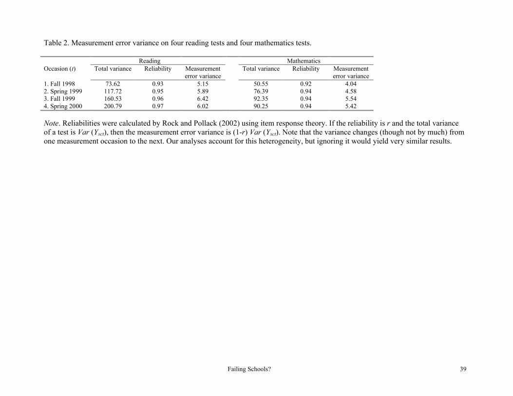
from test-reliability estimates in Rock and Pollack (2002); Table 2 reports the error variance for
reading and math tests on each of the four test occasions.
Table 2 near here
In vector form, the level 1 equation can be written concisely as
Ytcs = EXPOSUREStcs cs + etcs (1b),
where cs = [0cs 1cs 2cs 3cs]T and EXPOSUREStcs = [1 KINDERGARTENtcs SUMMERtcs FIRST GRADEtcs].
Then the level 2 equation models child-level variation within each school:
cs = s + ac (2)
where s = [0s 1s 2s 3s is the average achievement level and learning rates for school s; and ac =
[a0c a1c a2c a3c is a random effect representing the amount that child c deviates from the average for
school s.
Likewise, the level 3 equation models school-level variation between one school and another:
s = + bs (3)
where 0 = 00 01 02 03 is a fixed effect representing the grand average achievement level and
learning rates across all schools, and bs = [b0s b1s b2s b3s is a school-level random effect representing
the departure of school s from the grand average. The level 2 and 3 random effects ac and bs are
assumed to be multivariate normal variables with means of zero and unrestricted covariance matrices
of a and b.
The level 3 model can be expanded to include a vector of school characteristics XS:
s = + 1 Xs + bs (4)
Failing Schools? 18
where 1 is a coefficient matrix representing the fixed effects of the school characteristics in Xs,
including the school’s location (urban, rural, suburban) ethnic composition (percent minority),
poverty level (percent of students receiving free or reduced lunch), and sector (public, Catholic, other
religious, secular private).
Equations (1), (2), and (4) can be combined to give a mixed-model equation
Ytcs = EXPOSUREStcs (+ 1 Xs + bs + ac) + etcs (5),
which shows how differences in school learning rates are modeled using interactions between school
characteristics Xs and students’ EXPOSUREStcs to kindergarten, summer, and first grade.
This model has been used before (e.g., Downey, von Hippel, and Broh 2004). What is new in
this paper is the emphasis on two derived quantities:
1. Impact. The difference between the first-grade and summer learning rates. For school
s, impact is 4s3s – 2s.
2. 12-month learning. The average monthly learning rate over a period consisting of 2.4
months of summer followed by 9.6 months of first grade. For school s, 12-month
learning is )6.94.2( 32121
5 sss .
Average values for impact and 12-month learning can be obtained from any software that estimates
linear combinations of model parameters. To estimate the variances and correlations that involve
impact and 12-month learning, we carried out auxiliary calculations that are described in Appendix A.
MULTIPLE IMPUTATION
We compensated for missing values using a multiple-imputation strategy (Rubin 1987) that filled
in each missing value with ten plausible imputations. To account for correlations among tests on the
same child, the data were formatted so that each child’s test scores appeared on a single line alongside
Failing Schools? 19
the other variables (Allison 2002). To account for the interactions in equation (5), we multiplied the
component variables before imputation and imputed the resulting products like any other variable
(Allison 2002).6 To account for the difference between child- and school-level variables, we first
created a school-level file that included the school-level variables as well as school averages of the
child and test variables. We imputed this school file ten times, then merged the imputed school files
back with the observed child and test data.
Although our imputation model included test scores, none of the imputed test scores was used in
the analysis. Excluding imputations of the dependent variable is a strategy known as multiple
imputation, then deletion (MID), which increases efficiency and reduces biases resulting from
misspecification of the imputation model (von Hippel 2007). In this example, using the imputed test
scores in analysis would make little difference, since only 7% of test scores were missing within the
287 sampled schools.
Although we believe that our imputation strategy is sound, we recognize that alternatives are
possible. It is reassuring to note that we have analyzed these data using a variety of different
imputation strategies, without material effects on the results.
RESULTS
In this section, we compare school evaluation methods based on achievement, learning, and impact.
We focus on the results for reading. Results for mathematics, which were generally similar, are
available in Appendix B.
6 As is often the case, there was substantial collinearity between the interactions and the component variables. The imputation model compensated for this collinearity by using a ridge prior, as suggested by Schafer (1997).
Failing Schools? 20
Which Schools Are Failing?
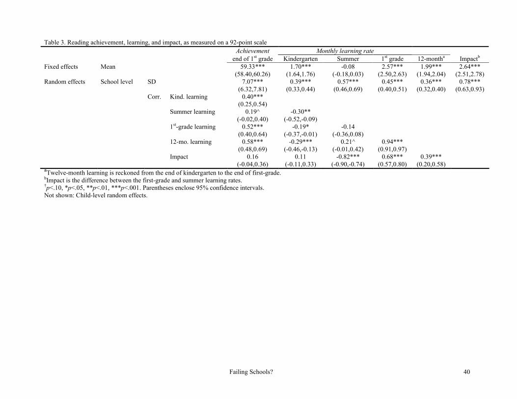
Table 3 summarizes the distribution of achievement, learning, and impact across the sampled schools.
At the end of first grade, the average achievement level is 59.33 points (out of 92). Children reach this
achievement level by learning at an average rate of 1.70 points per month during kindergarten, -0.08
points per month during summer, and 2.57 points per month during first grade. So school impact—the
difference between first-grade and summer learning rates—has an average value of 2.64 points per
month.7 In addition, 12-month learning—the average learning rate —is 2.57 points per month. Note
that, if we did not have seasonal data, we would have to use this 12-month (calendar year) learning
rate instead of the 9-month learning rate measured during the school year.
Table 3 near here
Of primary interest are the levels of agreement between different methods of evaluating
schools. If agreement is high, then the methods are more or less interchangeable and it does not matter
much whether we evaluate schools in terms of achievement, learning, or impact. If agreement is low,
on the other hand, then it is vital to know which method is best, since ideas about which schools are
failing (or succeeding) would then depend strongly on the yardstick by which schools are evaluated.
One way to evaluate agreement is to look at the school-level correlations. In general,
achievement is moderately correlated with school-year and 12-month learning rates, but only weakly
correlated with impact. For example, across schools, achievement (at the end of first grade) has a .52
correlation with the first-grade learning rate (95% CI: .40 to .64), and a .58 correlation with the 12-
month learning rate (95% CI: .48 to .69), but achievement has just a .16 correlation with impact (95%
CI: –.04 to .36).
7 2.57 minus -0.08 gives an impact of 2.65, but if values are not rounded before subtraction the value of impact is closer to 2.64.
Failing Schools? 21
Although these correlations are suggestive, they are somewhat abstract. To make differences
among the evaluation methods more concrete, let us suppose that every school were labeled as either
“failing” or “successful.” Of course, definitions of failure vary across states, complicating our attempt
to address this issue with national data. A useful exercise, however, is to suppose that a school is
“failing” if it is in the bottom quintile on a given criterion. The question, then, is: how often will a
school from the bottom quintile on one criterion also be in the bottom quintile on another? For
example, among schools with “failing” achievement levels, what percentage are failing with respect to
learning or impact? This percentage can be obtained by transforming the correlations in Table 3.8
Table 4 near here
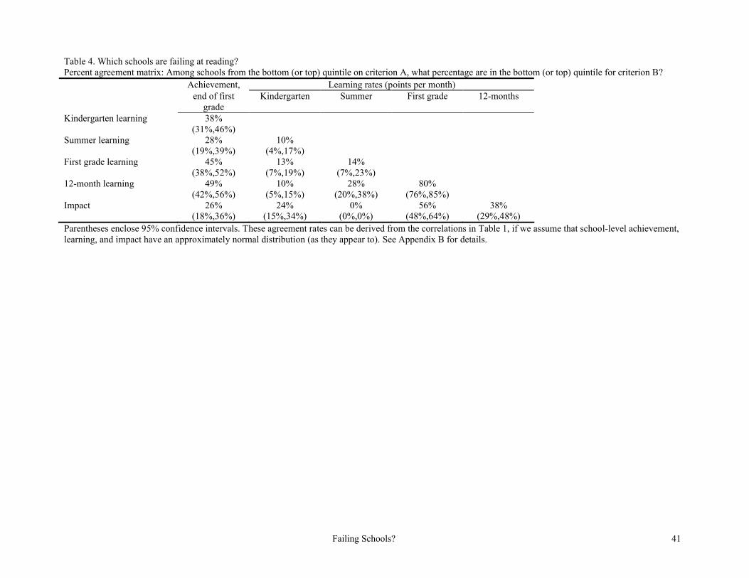
The estimated agreement levels are shown in Table 4. Again, evaluations based on
achievement agree only modestly with evaluations based on learning, and achievement agrees quite
poorly with impact. Among schools in the bottom quintile for achievement, only 49% (95% CI: 42%
to 56%) are in the bottom quintile for 12-month learning, only 45% (95% CI: 38% to 52%) are in the
bottom quintile for first-grade learning, and a mere 26% (95% CI: 18% to 36%) are in the bottom
quintile for impact. (The chance level of agreement would be 20%.) There were also substantial
disagreements between impact and learning; for example, among schools from the bottom quintile for
impact, only 56% (95% CI: 48% to 64%) were in the bottom quintile for first-grade learning, and only
38% (95% CI: 29% to 48%) were in the bottom quintile for 12-month learning.
8 The resulting percentages will be measures of latent school-level agreement, discounting random variation at the child and test levels. The transformation assumes that the different measures of school effectiveness have a multivariate normal distribution. (Scatterplots suggest that this assumption is reasonable.) Let (i, j) be standardized versions of two school-effectiveness measures, and let
84.q be the first quintile of the standard normal distribution. Then, given that i is in the bottom
quintile (i.e., s < q). the probability that j is also in the bottom quintile is pij = P(i<q | j<q) = 5 P(i<q, j<q) = 5 2(q, q, ij), where 2(q, q, ij) is the bivariate cumulative standard normal density with correlation ij, evaluated at (q, q) (Rose & Smith 2002). A confidence interval for pij is obtained by transforming the endpoints of a confidence interval for ij.
Failing Schools? 22
To illustrate the disagreements among evaluation methods, Figure 1 plots empirical Bayes
estimates (Raudenbush and Bryk 2002) of achievement, learning, and impact for the 287 schools in
our sample. The plots shows concretely how schools with failing achievement levels are often not
failing with respect to learning rates, and may even be above average with respect to impact.9
Conversely, a few schools that are succeeding with respect to achievement appear to be failing with
respect to learning or impact.
Figure 1 near here
What Kinds of Schools Are Failing?
What are the outward characteristics of low-performing schools? Conventional wisdom suggests that
failing schools tend to be urban public schools that serve predominantly poor or minority students.
But conventional wisdom is typically based on achievement scores. How might notions of school
performance be challenged if schools were evaluated in terms of learning or impact? Table 5 gives
the average characteristics of schools from the bottom and top four quintiles on empirical Bayes
estimates achievement, learning, and impact. The first column focuses on end-of-first-grade
achievement levels. Here the results fit the familiar pattern. Compared to other schools, schools from
the bottom achievement quintile tend to be public rather than private and urban rather than suburban
or rural. In addition, the students attending schools from the bottom achievement quintile are more
than twice as likely to come from minority groups and to qualify for free lunch programs.
Table 5 near here
When we evaluate schools on learning, however, socioeconomic differences between failing
and successful schools shrink or even disappear. For example, when schools are categorized on the
9 The agreement rates in Figure 2 differ slightly from those in Table 3. Figure 2 includes not only systematic disagreement due to differences among the evaluation criterion, but also random
Failing Schools? 23
basis of first-grade learning, kindergarten learning, or 12-month learning, schools from the bottom
quintile are not significantly more likely to be urban or public than are schools from the top four
quintiles. Students at schools that rank in the bottom quintile for learning are more likely to be poor
and minority than are students in the top four quintiles, but the ethnic and poverty differences when
schools are evaluated on learning are at least 10% smaller than they are when schools are evaluated on
achievement. When schools are evaluated on kindergarten learning, most of the socioeconomic
differences between bottom-quintile schools and other schools are not statistically significant.
When schools are evaluated with respect to impact, the association between school
characteristics and school failure is also weak—weaker than it is for first-grade or 12-month learning,
and almost as weak as it is for kindergarten learning. Under an impact criterion, schools from the
bottom quintile are not significantly more likely to be urban or public than are schools from the top
four quintiles, and low-impact schools do not have a disproportionate percentage of students who
qualify for free lunch. Low-impact schools do have a higher percentage of students from minority
groups (49% vs. 36% for the top four quintiles, p<.05), but the difference is about 10% smaller than it
is when schools are evaluated on first-grade learning or twelve-month learning, and 25% smaller than
it is when schools are evaluated on achievement.
Another way to examine school characteristics is to add school-level regressors to our
multilevel model of achievement, learning, and impact. We do this in Table 6, which shows again that
student disadvantage is more strongly associated with achievement than it is with learning or impact.
Specifically, Table 6 shows that school sector, school location, student poverty, and minority
enrollment explain 51% of the school-level variance in end-of-first-grade achievement levels, but
explain just 26% of the school-level variance in 12-month learning rates, 17% of the school-level
agreements and disagreements due to estimation error in the empirical Bayes estimates.
Failing Schools? 24
variance in first-grade learning rates, just 7% of the school-level variance in impact, and only 5% of
the school-level variance in kindergarten learning rates.
Table 6 near here
In short, when schools are evaluated with respect to achievement, schools serving
disadvantaged students are disproportionately likely to be labeled as “failing.” When schools are
evaluated in terms of learning or impact, however, school failure appears to be less concentrated
among disadvantaged groups.
IMPACT AS A MEASURE OF SCHOOL EFFECTIVENESS: REMAINING ISSUES
We have introduced impact as a potential replacement for the typically used achievement-based
measures of school effectiveness. Yet we recognize that evaluating schools via impact requires some
assumptions and raises several new questions.
First, the impact measure assumes that there is little “spillover” between seasons—i.e., that
school characteristics do not have important influences on summer learning. The literature on
spillover effects is limited, but the available evidence does suggest that spillover effects are minimal.
Georgies (2003) reported no relationship between summer learning and kindergarten teacher practices
or classroom characteristics. And in our own supplemental analyses of ECLS-K, we found that
summer learning rates were not higher if kindergarten teachers assigned summer book lists, or if
schools sent home preparatory “packages” before the beginning of first grade.
Second, the impact measure assumes that non-school influences on learning are similar during
the school year and during summer vacation. This assumption is more debatable. It seems plausible
that non-school effects might be smaller during the school year than during the summer, for the
obvious reason that during the school year children spend less time in their non-school environments.
This observation suggests the possibility of a weighted impact score that subtracts only a fraction of
Failing Schools? 25
the summer learning rate. The ideal weight to give summer is hard to know,10 but the results for
weighted impact would lie somewhere between the results for unweighted impact (which gives the
summer a weight of one) and the results for school-year learning (which gives the summer a weight of
zero). No matter where the results fell on this continuum, it would remain the case that the
characteristics of low-impact schools are quite different from those of low-achieving schools. That is,
compared to low-achievement schools, low-impact schools are not nearly as likely to be public, urban,
poor, or minority.11
An additional concern is that, even if impact is a more valid measure of effectiveness than
achievement, impact may also be less reliable. It is known that estimates of school learning rates are
less reliable than estimates of school achievement levels (Kane and Staiger 2002), and estimates of
impact are less reliable still. In a companion paper, however, we show that the increase in validity
more than compensates for the loss in reliability (von Hippel, under review). That is, a noisy measure
of learning is still a better reflection of school effectiveness than is a clean measure of achievement,
and a noisy measure of impact may be better still.
A final concern is that impact-based evaluation may penalize schools with high achievement.
It may be difficult for any school, no matter how good, to accelerate learning during the school year
10 An initially attractive possibility is to estimate the fraction by regressing the school-year learning rate on the summer learning rate. But since the correlation between school-year and summer learning is negative (Table 3), the estimated fraction would be negative as well, yielding an impact measure that is the sum rather than the difference of school and summer learning rates.11A more subtle possibility is that the non-school effect on learning varies across seasons and the seasonal pattern varies across schools serving different types of students. Suppose high-SES parents, for example, invest substantially in the summer but then relatively less so during the school year while low-SES parents produce the opposite seasonal pattern. This kind of scenario would produce biases in the impact measure, underestimating school impact for schools serving high-SES families and overestimating the performance of schools serving low-SES parents. Although little is known about this possible source of bias, most of what we know about parental involvement in children’s schooling suggests that this pattern is unlikely. Socioeconomically advantaged parents maintain active involvement in their children’s lives during the academic year by helping with homework, volunteering in classes, and attending school activities and parent-teacher conferences (Lareau 2002).
Failing Schools? 26
for high-achievement children. Our study, however, did not find a negative correlation between
impact and achievement; to the contrary, the correlation between achievement and impact was
positive, though small (Table 3). Among schools in the top quintile on achievement, 26% were also
in the top quintile on impact (Table 4), suggesting that it is quite possible for a high-achieving school
to be high-impact as well.
While the assumptions of impact-based evaluation are nontrivial, we should bear in mind that
every school-evaluation measure makes assumptions. The assumptions needed for the impact measure
should be compared to those required to treat achievement or learning as measures of school
performance. As previously noted, evaluation systems based on achievement or learning models
assume that non-school factors play a relatively minor role in shaping student outcomes. This
assumption is badly wrong for achievement, and somewhat wrong for learning.
DISCUSSION
Confidently identifying “failing” schools requires a method of evaluation that is sociologically
informed—that is, a method recognizing that children’s cognitive development is a function of
exposure to multiple social contexts. The simple observation that children are influenced in important
ways by their non-school environments undermines achievement-based methods for evaluating
schools. While holding schools accountable for their performance is attractive for many reasons,
schools cannot reasonably be held responsible for what happens to children outside of school.
Other scholars have made this same observation, and have proposed alternatives to
achievement-based assessment by using annual learning rates, or by “adjusting” achievement levels
for schools’ socioeconomic characteristics. We have already discussed the practical, theoretical, and
political difficulties of these alternatives. Our contribution is a novel solution. By employing seasonal
data we can evaluate schools in terms of impact—separating the effects of the school and non-school

Failing Schools? 27
environments without having to measure either environment directly. We suggest that impact can be
an important part of the continuing discussion on measuring school effectiveness.
We have argued that there are conceptual reasons for preferring impact over achievement, and
even over learning-based measures of school effectiveness. If we are right that achievement is the
least valid measure of school effectiveness, then our results suggest substantial error in the way
schools are currently evaluated. Indeed, our analyses indicate that, more often than not, schools
vulnerable to the “failing” label under achievement standards were not among the least effective
schools. Specifically, among schools from the bottom quintile for achievement, we found that less
than half are in the bottom quintile for learning, and only a quarter are in the bottom quintile for
impact. In these mislabeled schools, students have low achievement levels, but they are learning at a
reasonable rate, and they are learning substantially faster during the school year than during summer
vacation. These patterns suggest that many so-called “failing” schools are having at least as much
impact on their students’ learning rates as are schools with much higher achievement scores.
We should emphasize that our results do not suggest that all schools have similar impact. To
the contrary, impact varies even more across schools than does achievement or learning. For impact,
the between-school coefficient of variation is 30%; that is, the between-school standard deviation is
30% of the mean. For learning rates, by contrast, the coefficient of variation is just 23% in
kindergarten and 18% in first grade, and for end-of-first-grade achievement, the coefficient of
variation is just 12%. So schools do vary substantially in impact, but variation in impact is not
strongly associated with sector, location, or student body characteristics. Whereas high-achieving
schools are concentrated among the affluent, high-impact schools exist in communities of every kind.
For example, in schools serving disadvantaged students, despite scarce resources, high teacher
turnover, and low parental involvement, a sizable number of teachers and administrators are having
considerable impact—much more impact than previously thought. When we measure school
Failing Schools? 28
effectiveness fairly, the results highlight how a school serving the disadvantaged can have tremendous
impact even if it does not raise its students’ skills to a determined proficiency level.
Our results raise serious concerns about current methods used to hold schools accountable for
their students’ achievement levels. Because achievement-based evaluation is biased against schools
serving the disadvantaged, evaluating schools on the basis of achievement may actually undermines
the NCLB goal of reducing racial/ethnic and socioeconomic performance gaps. If schools serving the
disadvantaged are evaluated on a biased scale, their teachers and administrators may respond like
workers in other industries when they are evaluated unfairly; the typical response to unfair evaluations
is frustration, reduced effort, and attrition (Hodson 2001). Our call is not to make excuses for schools
serving disadvantaged populations, but rather to ask that all schools be given an equal chance to
succeed. Under a fair system, a school’s chances of receiving a high mark should not depend on the
kinds of students it happens to serve.
It is not impractical to make school evaluation systems fairer. Currently, NCLB requires once-
a-year testing in grades 3-8. These tests are typically used to rank schools based on achievement, but
the availability of annual test scores makes it possible to rank schools based on the amount learned in
a 12-month calendar year. Although these 12-month learning rates include summer learning as well as
school-year learning, our results suggest that rankings based on 12-month rankings are not
substantially different from rankings based on 9-month learning.
Rankings based on learning rates, however, can differ substantially from rankings based on
impact, and measuring impact requires seasonal rather than annual data. At first glance, collecting
seasonal data would seem to require doubling the number of annual tests—an unattractive option for
most policymakers, school personnel, taxpayers, and parents. As a practical alternative, though,
schools could maintain the same number of assessments but alter their timing. NCLB currently
requires tests at the ends of grades 3-8; but these six tests could be rescheduled for the end of third
Failing Schools? 29
grade and the beginning and end of fourth grade, and then for the end of seventh grade and the
beginning and end of eighth grade. Such a schedule would allow school evaluators to estimate impact
and school-year learning during fourth grade and eighth grade without increasing the number of tests.
Valid information about these two school years would be preferable to the six years of low-validity
achievement levels that are currently provided.
We have argued that achievement-based systems have important limitations when the goal is
to hold schools accountable. But for other reasons it may still be useful to maintain publicly available
information on achievement. For example, if our interest shifts from identifying “failing” schools to
locating disadvantaged schools with the greatest potential for improvement, it may be useful to have
information on both achievement and impact. High-impact schools with low achievement levels
might be especially attractive schools in which to invest additional resources, given that they appear
to be operating efficiently. Learning more about the details of what goes on in these high-impact
schools is an important next step.
The validity of school performance measures is critical to the success of market-based
education reforms because making information about school quality publicly available is supposed to
pressure school personnel to improve. But our results suggest that the information currently available
regarding school quality is substantially flawed, undermining the development of market pressures as
a mechanism for improving American schools. Poor information reduces market efficiency by too
often sending parents away from effective schools that serve children from disadvantaged
backgrounds and insufficiently pressuring ineffective schools that serve children from advantaged
backgrounds. Our results suggest that the magnitude of the error is substantial; indeed, current
accountability systems relying on achievement may do as much to undermine school quality as they
do to promote it.
Failing Schools? 30
REFERENCES
Agresti, A. 2002. Categorical Data Analysis. New York: Wiley.
Allison, Paul D. 2002. Missing Data. Thousand Oaks, CA: Sage.
Allison, Paul D. 2005. "Imputation of Categorical Variables With PROC MI." SAS Users Group
International, 30th Meeting (SUGI 30) (Philadelphia, PA.
Black, Sandra (1999). “Do Better Schools Matter? Parental Valuation of Elementary Education.”
Quarterly Journal of Economics 114(2): 577-599.
Bliss, J. R. 1991. Pp. 43-57 in Rethinking Effective Schools: Research and Practice. Bliss, J. R., W.
A. Firestone, C. E. Richards, Eds. Englewood Cliffs, NJ : Prentice Hall.
Bollen, Kenneth A. (1989). Structural Equations with Latent Variables. New York: Wiley.
Booher-Jennings, Jennifer Lee. 2004. “Responding to the Texas Accountability System: The Erosion
of Relational Trust.” Paper presented at the Annual Meetings of the American Sociological
Association, San Fransisco.
Boyd, D., Lankford, H., Loeb, S., and Wyckoff, J. 2005. “The Draw of Home: How Teachers’
Preferences for Proximity Disadvantage Urban Schools.” Journal of Policy Analysis and
Management 24:113-132.
Brooks-Gunn, Jeanne, Greg J. Duncan, and J. Lawrence Aber. 1997. Neighborhood Poverty: Context
and Consequences for Children. New York: Russell Sage Foundation.
Chatterji, Madhabi. 2002. “Models and Methods for Examining Standards-Based Reforms and
Accountability Initiatives: Have the Tools of Inquiry Answered Pressing Questions on
Improving Schools?” Review of Educational Research 72(3): 345-86.
Chubb, John, and Terry Moe. 1990. Politics, Markets, and America’s Schools. Washington, D.C.:
Brookings Institution Press.
Failing Schools? 31
Crouse, James, and Dale Trusheim. 1988. The Case against the SAT. University of Chicago Press.
Deming, W. Edwards. 2000. The New Economics: For Industry, Government, Education (2nd ed.,
MIT Press)
Denton, Kristin and Jerry West. 2002. Children’s Reading and Mathematics Achievement in
Kindergarten and First Grade, NCES 2002-125. Washington DC: U.S. Department of
Education, National Center for Education Statistics.
Downey, Douglas B. 1995. “When Bigger is Not Better: Family Size, Parental Resources, and
Children’s Educational Performance.” American Sociological Review 60:747-761.
Downey, Douglas B., Paul T. von Hippel, and Beckett Broh. 2004. “Are Schools the Great
Equalizer? Using Seasonal Comparisons to Assess Schooling’s Role in Inequality.” Paper
presented at the American Sociological Association Meetings in Chicago, IL.
Entwisle, Doris R. and Karl L. Alexander. 1992. “Summer Setback: Race, Poverty, School
Composition and Math Achievement in the First Two Years of School.” American
Sociological Review 57:72-84.
Entwisle, Doris R. and Karl L. Alexander. 1994. “The gender gap in math: Its possible origins in
neighborhood effects.” American Sociological Review 59:822-838.
Georgies, Annie. 2003. “Explaining Divergence in Rates of Learning and Forgetting among First
Graders.” Paper presented at the American Sociological Association Meetings in Atlanta.
Grissmer, David. (2002). “Comment [on Kane and Staiger 2002]” Pp. 269-272 in Diane Ravitch (ed.),
Brookings Papers on Education Policy. Washington, DC: Brookings Institution.
Hart, Betty and Todd R. Risley. 1995. Meaningful Differences in the Everyday Experiences of
Young American Children. The University of Kansas: Paul H. Brookes Publishing Co.
Harville, David. 1997. Matrix Algebra from a Statistician’s Perspective. New York: Springer.
Heyns, Barbara. 1978. Summer learning and the effects of schooling. New York: Academic Press.
Failing Schools? 32
-----.1987. “Schooling and cognitive development: Is there a season for learning?” Child Development
58:1151-1160.
Hodson, Randy. 2001. Dignity at Work. New York: Cambridge University Press.
Hofferth, Sandra L., and John F. Sandberg (2001). “How American children spend their time.”
Journal of Marriage and the Family, 63(2), 295-308.
Holme, Jennifer Jellison. 2002. “Buying Homes, Buying Schools: School Choice and the Social
Construction of School Quality.” Harvard Educational Review 72:139-167.
Horton, Nicholas J., Stuart R. Lipsitz, and Michael Parzen. 2003. "A Potential for Bias When
Rounding in Multiple Imputation." The American Statistician 57(4):229-32.
Hu, D. 2000. “The Relationship of School Spending and Student Achievement When Achievement is
Measured by Value-Added Scores.” Ph.D. dissertation. Nashville, TN: Vanderbilt University.
Jencks, Christopher, Marshall Smith, Henry Acland, Mary Jo Bane, David Cohen, Herbert Gintis,
Barbara Heyns, and Stephan Michelson. 1972. Inequality: A Reassessment of the Effect of
Family and Schooling in America. Basic Books: New York.
Jencks, Christopher. 1998. “Racial Bias in Testing,” Pp. 55-85 in The Black-White Test Score Gap.
Washington, DC: Brookings Institution Press.
Johnson, Richard A., and Dean W. Wichern. 1997. Applied Multivariate Statistical Analysis (4th ed.).
Upper Saddle River, NJ: Prentice-Hall.
Kane, Thomas J., and Douglas O. Staiger. (2002). “Volatility in School Test Scores: Implications for
Test-Based Accountability Systems.” Pp. 235-269 in Diane Ravitch (ed.), Brookings Papers
on Education Policy. Washington, DC: Brookings Institution.
Kupermintz, H. 2002. “Value-Added Assessment of Teachers: The Empirical Evidence.” Pp. 217-234
in School Reform Proposals: The Research Evidence. Alex Molnar, Ed. Greenwich, CT:
Information Age Publishing.
Failing Schools? 33
Ladd, Helen F. 2002. Market-Based Reforms in Urban Education. Washington, DC. Economic Policy
Institute.
Ladd, Helen F. and Randall P. Walsh. 2002. “Implementing value-added measures of school
effectiveness: getting the incentives right.” Economics of Education Review 21:1-27.
Ladd, Helen. (2002). “Comment [on Kane and Staiger 2002]” Pp. 273-283 in Diane Ravitch (ed.),
Brookings Papers on Education Policy. Washington, DC: Brookings Institution.
Lareau, Annette. 2000. Home Advantage: Social Class and Parental Intervention in Elementary
Education. Oxford: Rowman and Littlefield.
Lee, Valerie E. and David T. Burkam. 2002. Inequality at the Starting Gate: Social Background
Differences in Achievement as Children Begin School. Economic Policy Institute:
Washington, DC.
Little, Roderick J. A. 1992. “Regression With Missing X's: A Review.” Journal of the American
Statistical Association 87(420):1227-37.
Louis, K. S. and M. B. Miles. 1991. “Managing Reform: Lessons From Urban High Schools.”
School Effectiveness and School Improvement 2(1):75-96.
McLanahan, Sara, and Gary Sandefur. 1994. Growing Up with a Single Parent: What Hurts, What
Helps?
Meng, X. L. “Multiple Imputation Inferences With Uncongenial Sources of Input.” Statistical Science
10:538-73.
Meyer, Robert H. 1996. “Value-Added Indicators of School Performance.” Pp. 197-223 in Improving
America’s Schools: The Role of Incentives (Eds. Eric A. Hanushek and Dale W. Jorgenson).
National Academy Press: Washington DC.
Failing Schools? 34
Mortimore, P. 1991. “Effective Schools From a British Perspective: Research and Practice. Pp. 76-
90 in Rethinking effective schools : research and practice. Bliss, J. R., W. A. Firestone, C. E.
Richards, Eds. Englewood Cliffs, NJ: Prentice.
National Center for Education Statistics. 2003. Early Childhood Longitudinal Survey, Kindergarten
Cohort [. Washington, DC.
National Center for Education Statistics. User's Manual for the ECLS-K Longitudinal Kindergarten-
First Grade Public-Use Data Files and Electronic Codebook. Washington, DC: U.S.
Department of Education.
Newmann, F. M. 1991. “Student Engagement in Academic Work: Expanding the Perspective on
Secondary School Effectiveness.” Pp. 58-75 in Rethinking effective schools : research and
practice. Bliss, J. R., W. A. Firestone, C. E. Richards, Eds. Englewood Cliffs, NJ: Prentice
Hall.
Raudenbush, S. W. and A. S. Bryk. (2002). Hierarchical Linear Models: Applications and Data
Analysis Methods. 2 ed. Thousand Oaks, CA: Sage.Raudenbush, Stephen W. and Anthony S.
Bryk. 2002b. Hierarchical Linear Models: Applications and Data Analysis Methods. 2 ed.
Thousand Oaks, CA: Sage.
Raudenbush, Stephen W., and Anthony S. Bryk. 2002. Hierachical Linear Models: Applications and
Data Analysis Methods (2nd ed.). Thousand Oaks, CA: Sage.
Reardon, Sean. 2003. “Sources of Educational Inequality” Paper presented at the American
Sociological Association Meetings in Atlanta, Georgia.
Renzulli Linda A., and Vincent J. Roscigno. 2005. “Charter School Policy, Implementation, and
Diffusion Across the United States.” Sociology of Education 78:344-366.
Robinson, G. K. 1991. “That BLUP Is a Good Thing: The Estimation of Random Effects.” Statistical
Science 6(1):15-32.
Failing Schools? 35
Rock, Donald A. and Judith M. Pollack. 2002. “Early Childhood Longitudinal Study—Kindergarten
Class of 1998-99 (ECLS-K), Psychometric Report for Kindergarten through First Grade.”
Washington, DC: U.S. Department of Education, National Center for Education Statistics.
Rock, Donald A. and Judith M. Pollack. Early Childhood Longitudinal Study - Kindergarten Class of
1998-99 (ECLS-K), Psychometric Report for Kindergarten Through First Grade. NCES
200205. Washington, DC: National Center for Education Statistics.
Rose, Colin, and Murray D. Smith. 2002. Mathematical Statistics with Mathematica. New York:
Springer.
Rothstein, Richard. 2004. Class and Schools Using Social, Economic, and Educational Reform to
Close the Black-White Achievement Gap. Economic Policy Institute.
Rowan, B. 1984. “Shamanistic Rituals in Effective Schools.” Issues in Education 2:517:37.NCES
200205. Washington, DC: National Center for Education Statistics.
Rubenstein, Ross, Leanna Stiefel, Amy Ellen Schwartz, and Hella Bel Hadj Amor. “Distinguishing
Good Schools From Bad In Principle and Practice: A Comparison of Four Methods.” Pp. 55-
70 in Fowler, W.J., Jr., ed. (2004) Developments in School Finance: Fiscal Proceedings from
the Annual State Data Conference of July 2003, (NCES 2004-325), U.S. Department of
Education, National Center for Education Statistics, Washington, DC: Government Printing
office.
Rubin, Donald B. 1987. Multiple Imputation for Survey Nonresponse. New York: Wiley.
Ryan, James E. 2004. “The Perverse Incentives of the No Child Left Behind Act.” New York
University Law Review 79:932-989.
Sanders, W.L., and J.P. Horn. 1998. “Research Findings from the Tennessee Value Added
Assessment System (TVAAS) Database: Implications for Educational Evaluation and
Research.” Journal of Personnel Evaluation in Education 12(3), 247-256.
Failing Schools? 36
Sanders, W.L. 1998. “Value-Added Assessment.” The School Administrator 55(11): 24-32.
Schafer, J. L. 1997. Analysis of Incomplete Multivariate Data. Boca Raton, FL: Chapman and Hall.
Schafer, J. L. and R. M. Yucel. 2002. “Computational Strategies for Multivariate Linear Mixed-
Effects Models With Missing Values.” Journal of Computational & Graphical Statistics
11(2):437-57.
Schafer, Joseph L. 1997. Analysis of Incomplete Multivariate Data. Boca Raton, FL: Chapman and
Hall.
Schafer, Joseph L., and Recai M. Yucel. 2002. “Computational Strategies for Multivariate Linear
Mixed-Effects Model With Missing Values.”
Scheerens, Jaap. and Bosker, R. 1997. The Foundations of Educational Effectiveness Oxford:
Elsevier Science Ltd.
Singer, Judith D. and John B. Willett. 2003. Applied Longitudinal Data Analysis: Modeling Change
and Event Occurrence. Oxford, UK: Oxford University Press.
Teachman, Jay. 1987. “Family Background, Educational Resources, and Educational Attainment,”
American Sociological Review 52:548-57.
Teddlie, Charles, and David Reynolds. 1999. The International Handbook of School Effectiveness
Research: An International Survey of Research on School Effectivenss. London: Falmer
Press.
Thernstrom, Abigail and Stephan Thernstrom. 2003. No Excuses: Closing the Racial Gap in
Learning. New York, New York: Simon A& Schuster.
von Hippel, P.T. 2004. “School Accountability [a comment on Kane and Staiger (2002)].” Journal of
Economic Perspectives, 18(2), 275-276.
von Hippel, Paul T. 2007. “Regression with Missing Y’s: An Improved Strategy for Analyzing
Multiply Imputed Data.” Sociological Methodology 37(1), 83-117.
Failing Schools? 37
von Hippel, Paul T. Under review. “Achievement, Learning, and Seasonal Impact as Measures of
School Effectiveness: It’s Better To Be Valid Than Reliable.”
Walberg, Herbert J. 1984. “Families as Partners in Educational Productivity.” Phi Delta Kappan
65:397-400.
West, J., K. Denton, and E. Germino-Hausken. 2000. America’s Kindergartners: Findings from the
Early Childhood Longitudinal Study, Kindergarten Class of 1998-99, NCES 2000-070.
Washington DC: U.S. Department of Education, National Center for Education Statistics.
West, Martin R. and Paul E. Peterson. 2003. “The Politics and Practice of Accountability.” Pp. 1-20
in No Child Left Behind: The Politics and Practice of School Accountability (Peterson and
West Eds.) Washington, DC: The Brookings Institution.
Wilson, William Julius. 1996. When Work Disappears: The World of the New Urban Poor. New
York: Knopf.
Winship, Christopher, and Stephen L. Morgan. 1999. “The Estimation of Causal Effects from
Observational Data.” Annual Review of Sociologgy. 25, 659-707.
This is the accepted version. For the published version, see the July 2008 issue of Sociology of Education.
Table 1. Proportion of Waking Hours That Children Spend in School
From birth to age 18 One calendar year One academic year
Hours in school/day --- 7 7
School days attended/year --- 180 180
Hours awake/day --- 14 14
Hours in school/year --- 1,260 1,260
Hours awake/year---
(14 hours/day X 365 days)
= 5,110
(14 hours/day X 285 days)
= 3,990Proportion of waking hours in school
.13 (1,260 hours/year)/(5,110 hours/year)
= .25
(1,260 hours/year)/(3,990 hours/year)
= .32Source Walberg (1984) Authors’ calculations Authors’ calculations
Failing Schools? 39
Table 2. Measurement error variance on four reading tests and four mathematics tests.
Reading MathematicsOccasion (t) Total variance Reliability Measurement
error varianceTotal variance Reliability Measurement
error variance1. Fall 1998 73.62 0.93 5.15 50.55 0.92 4.042. Spring 1999 117.72 0.95 5.89 76.39 0.94 4.583. Fall 1999 160.53 0.96 6.42 92.35 0.94 5.544. Spring 2000 200.79 0.97 6.02 90.25 0.94 5.42
Note. Reliabilities were calculated by Rock and Pollack (2002) using item response theory. If the reliability is r and the total variance of a test is Var (Ysct), then the measurement error variance is (1-r) Var (Ysct). Note that the variance changes (though not by much) from one measurement occasion to the next. Our analyses account for this heterogeneity, but ignoring it would yield very similar results.
Failing Schools? 40
Table 3. Reading achievement, learning, and impact, as measured on a 92-point scaleAchievement Monthly learning rate
end of 1st grade Kindergarten Summer 1st grade 12-montha Impactb
Fixed effects Mean 59.33***(58.40,60.26)
1.70***(1.64,1.76)
-0.08(-0.18,0.03)
2.57***(2.50,2.63)
1.99***(1.94,2.04)
2.64***(2.51,2.78)
Random effects School level SD 7.07***(6.32,7.81)
0.39***(0.33,0.44)
0.57***(0.46,0.69)
0.45***(0.40,0.51)
0.36***(0.32,0.40)
0.78***(0.63,0.93)
Corr. Kind. learning 0.40***(0.25,0.54)
Summer learning 0.19^(-0.02,0.40)
-0.30**(-0.52,-0.09)
1st-grade learning 0.52***(0.40,0.64)
-0.19*(-0.37,-0.01)
-0.14(-0.36,0.08)
12-mo. learning 0.58***(0.48,0.69)
-0.29***(-0.46,-0.13)
0.21^(-0.01,0.42)
0.94***(0.91,0.97)
Impact 0.16(-0.04,0.36)
0.11(-0.11,0.33)
-0.82***(-0.90,-0.74)
0.68***(0.57,0.80)
0.39***(0.20,0.58)
aTwelve-month learning is reckoned from the end of kindergarten to the end of first-grade.bImpact is the difference between the first-grade and summer learning rates.†p<.10, *p<.05, **p<.01, ***p<.001. Parentheses enclose 95% confidence intervals.Not shown: Child-level random effects.
Failing Schools? 41
Table 4. Which schools are failing at reading? Percent agreement matrix: Among schools from the bottom (or top) quintile on criterion A, what percentage are in the bottom (or top) quintile for criterion B?
Achievement, Learning rates (points per month)end of first
gradeKindergarten Summer First grade 12-months
Kindergarten learning 38%(31%,46%)
Summer learning 28%(19%,39%)
10%(4%,17%)
First grade learning 45%(38%,52%)
13%(7%,19%)
14%(7%,23%)
12-month learning 49%(42%,56%)
10%(5%,15%)
28%(20%,38%)
80%(76%,85%)
Impact 26%(18%,36%)
24%(15%,34%)
0%(0%,0%)
56%(48%,64%)
38%(29%,48%)
Parentheses enclose 95% confidence intervals. These agreement rates can be derived from the correlations in Table 1, if we assume that school-level achievement, learning, and impact have an approximately normal distribution (as they appear to). See Appendix B for details.
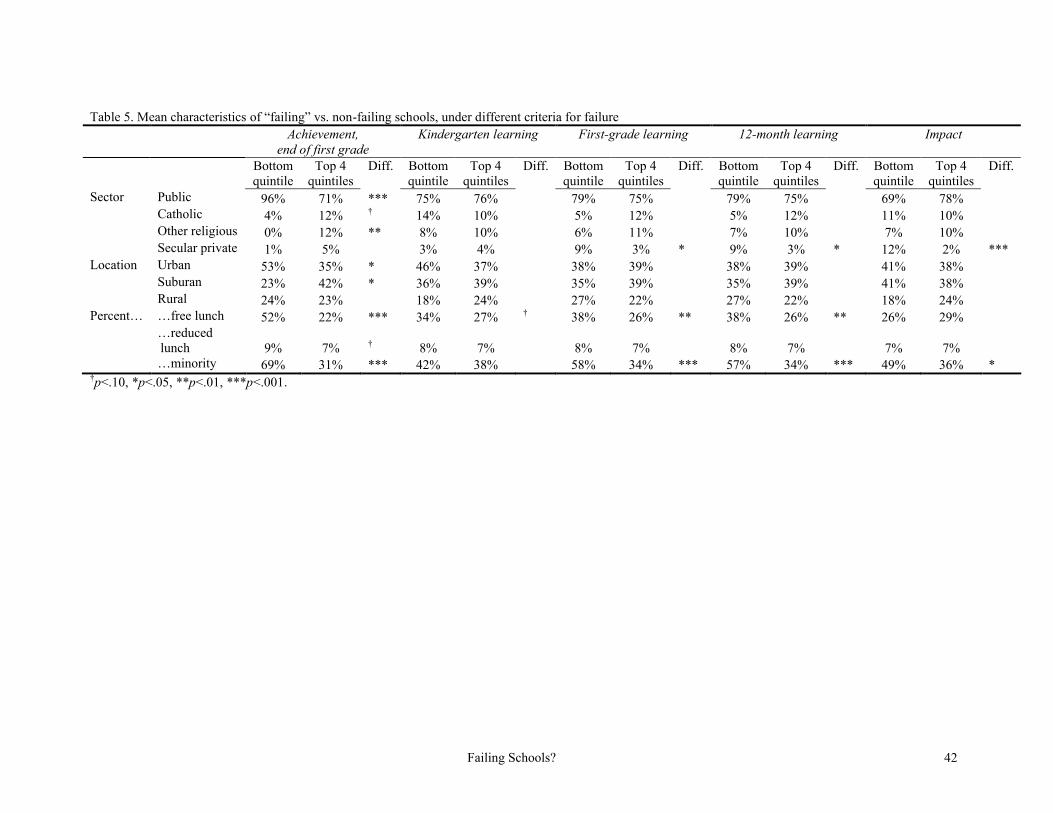
Failing Schools? 42
Table 5. Mean characteristics of “failing” vs. non-failing schools, under different criteria for failureAchievement,
end of first gradeKindergarten learning First-grade learning 12-month learning Impact
Bottomquintile
Top 4quintiles
Diff. Bottomquintile
Top 4quintiles
Diff. Bottomquintile
Top 4quintiles
Diff. Bottomquintile
Top 4quintiles
Diff. Bottomquintile
Top 4quintiles
Diff.
Sector Public 96% 71% *** 75% 76% 79% 75% 79% 75% 69% 78%Catholic 4% 12% † 14% 10% 5% 12% 5% 12% 11% 10%Other religious 0% 12% ** 8% 10% 6% 11% 7% 10% 7% 10%Secular private 1% 5% 3% 4% 9% 3% * 9% 3% * 12% 2% ***
Location Urban 53% 35% * 46% 37% 38% 39% 38% 39% 41% 38%Suburan 23% 42% * 36% 39% 35% 39% 35% 39% 41% 38%Rural 24% 23% 18% 24% 27% 22% 27% 22% 18% 24%
Percent… …free lunch 52% 22% *** 34% 27% † 38% 26% ** 38% 26% ** 26% 29%…reduced lunch 9% 7% † 8% 7% 8% 7% 8% 7% 7% 7%…minority 69% 31% *** 42% 38% 58% 34% *** 57% 34% *** 49% 36% *
†p<.10, *p<.05, **p<.01, ***p<.001.
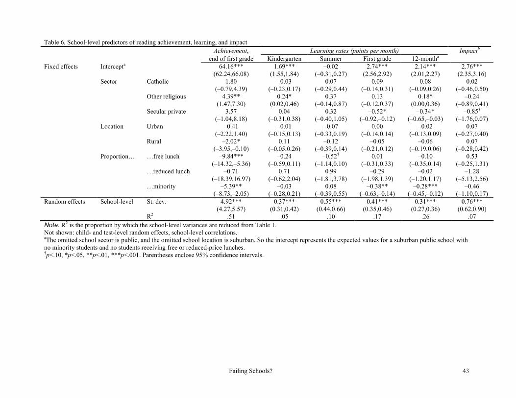
Failing Schools? 43
Table 6. School-level predictors of reading achievement, learning, and impact Achievement, Learning rates (points per month) Impactb
end of first grade Kindergarten Summer First grade 12-montha
Fixed effects Intercepta 64.16***(62.24,66.08)
1.69***(1.55,1.84)
–0.02(–0.31,0.27)
2.74***(2.56,2.92)
2.14***(2.01,2.27)
2.76***(2.35,3.16)
Sector Catholic 1.80(–0.79,4.39)
–0.03(–0.23,0.17)
0.07(–0.29,0.44)
0.09(–0.14,0.31)
0.08(–0.09,0.26)
0.02(–0.46,0.50)
Other religious 4.39**(1.47,7.30)
0.24*(0.02,0.46)
0.37(–0.14,0.87)
0.13(–0.12,0.37)
0.18*(0.00,0.36)
–0.24(–0.89,0.41)
Secular private 3.57(–1.04,8.18)
0.04(–0.31,0.38)
0.32(–0.40,1.05)
–0.52*(–0.92,–0.12)
–0.34*(–0.65,–0.03)
–0.85†
(–1.76,0.07)Location Urban –0.41
(–2.22,1.40)–0.01
(–0.15,0.13)–0.07
(–0.33,0.19)0.00
(–0.14,0.14)–0.02
(–0.13,0.09)0.07
(–0.27,0.40)Rural –2.02*
(–3.95,–0.10)0.11
(–0.05,0.26)–0.12
(–0.39,0.14)–0.05
(–0.21,0.12)–0.06
(–0.19,0.06)0.07
(–0.28,0.42)Proportion… …free lunch –9.84***
(–14.32,–5.36)–0.24
(–0.59,0.11)–0.52†
(–1.14,0.10)0.01
(–0.31,0.33)–0.10
(–0.35,0.14)0.53
(–0.25,1.31)…reduced lunch –0.71
(–18.39,16.97)0.71
(–0.62,2.04)0.99
(–1.81,3.78)–0.29
(–1.98,1.39)–0.02
(–1.20,1.17)–1.28
(–5.13,2.56)…minority –5.39**
(–8.73,–2.05)–0.03
(–0.28,0.21)0.08
(–0.39,0.55)–0.38**
(–0.63,–0.14)–0.28***
(–0.45,–0.12)–0.46
(–1.10,0.17)Random effects School-level St. dev. 4.92***
(4.27,5.57)0.37***
(0.31,0.42)0.55***
(0.44,0.66)0.41***
(0.35,0.46)0.31***
(0.27,0.36)0.76***
(0.62,0.90)R2 .51 .05 .10 .17 .26 .07
Note. R2 is the proportion by which the school-level variances are reduced from Table 1. Not shown: child- and test-level random effects, school-level correlations.aThe omitted school sector is public, and the omitted school location is suburban. So the intercept represents the expected values for a suburban public school with no minority students and no students receiving free or reduced-price lunches.†p<.10, *p<.05, **p<.01, ***p<.001. Parentheses enclose 95% confidence intervals.
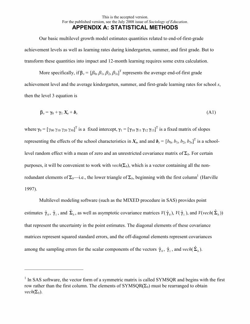
This is the accepted version. For the published version, see the July 2008 issue of Sociology of Education.
APPENDIX A: STATISTICAL METHODS
Our basic multilevel growth model estimates quantities related to end-of-first-grade
achievement levels as well as learning rates during kindergarten, summer, and first grade. But to
transform these quantities into impact and 12-month learning requires some extra calculation.
More specifically, if s = [0s 1s 2s 3s represents the average end-of-first grade
achievement level and the average kindergarten, summer, and first-grade learning rates for school s,
then the level 3 equation is
s = + 1 Xs + bs (A1)
where 0 = 00 10 20 30 is a fixed intercept,1 = 10 11 12 13 is a fixed matrix of slopes
representing the effects of the school characteristics in Xs, and and bs = [b0s b1s b2s b3s is a school-
level random effect with a mean of zero and an unrestricted covariance matrix of b. For certain
purposes, it will be convenient to work with vech(b), which is a vector containing all the non-
redundant elements of b—i.e., the lower triangle of b, beginning with the first column (Harville
1997).
Multilevel modeling software (such as the MIXED procedure in SAS) provides point
estimates 0γ̂ , 1γ̂ , and bΣ̂ , as well as asymptotic covariance matrices V( 0γ̂ ), V( 1γ̂ ), and V(vech( bΣ̂ ))
that represent the uncertainty in the point estimates. The diagonal elements of these covariance
matrices represent squared standard errors, and the off-diagonal elements represent covariances
among the sampling errors for the scalar components of the vectors 0γ̂ , 1γ̂ , and vech( bΣ̂ ).
1In SAS software, the vector form of a symmetric matrix is called SYMSQR and begins with the first row rather than the first column. The elements of SYMSQRb) must be rearranged to obtain vech(b).
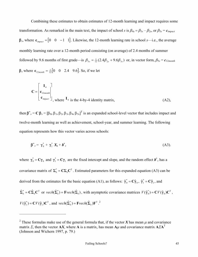
Failing Schools? 45
Combining these estimates to obtain estimates of 12-month learning and impact requires some
transformation. As remarked in the main text, the impact of school s is 4s3s – 2s, or 5s = cimpact
s, where 1100 impactc . Likewise, the 12-month learning rate in school s—i.e., the average
monthly learning rate over a 12-month period consisting (on average) of 2.4 months of summer
followed by 9.6 months of first grade—is )6.94.2( 32121
5 sss or, in vector form, 5s = c12month
s where 6.94.200121
12 monthc . So, if we let
impact
month
c
c
I
C 12
4
, where 4I is the 4-by-4 identity matrix, (A2),
then s = C s = [0s 1s 2s 3s 4s 5s is an expanded school-level vector that includes impact and
twelve-month learning as well as achievement, school-year, and summer learning. The following
equation represents how this vector varies across schools:
s =*0γ + *
1γ Xs + bs (A3).
where 0*0 Cγγ and 1
*1 Cγγ are the fixed intercept and slope, and the random effect bs has a
covariance matrix of T* CCΣΣ bb . Estimated parameters for this expanded equation (A3) can be
derived from the estimates for the basic equation (A1), as follows: 0*0 ˆˆ γCγ , 1
*1 ˆˆ γCγ , and
T* ˆˆ CΣCΣ bb or )ˆ()ˆ( *bb vechvech ΣFΣ , with asymptotic covariance matrices T
0*0 )ˆ()ˆ( CγCγ VV ,
T1
*1 )ˆ()ˆ( CγCγ VV , and T* )ˆ()ˆ( FΣFΣ bb vechvech .2
2 These formulas make use of the general formula that, if the vector X has mean and covariance matrix , then the vector AX, where A is a matrix, has mean A and covariance matrix AAT
(Johnson and Wichern 1997, p. 79.)
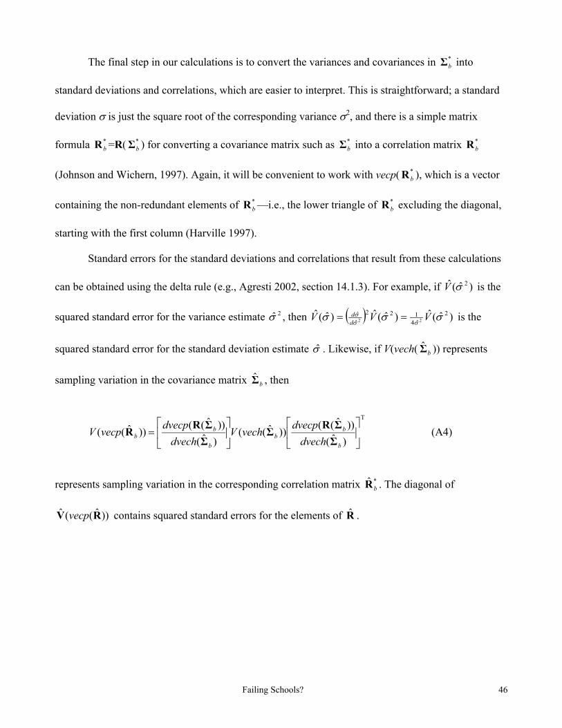
Failing Schools? 46
The final step in our calculations is to convert the variances and covariances in *bΣ into
standard deviations and correlations, which are easier to interpret. This is straightforward; a standard
deviation is just the square root of the corresponding variance 2, and there is a simple matrix
formula *bR =R( *
bΣ ) for converting a covariance matrix such as *bΣ into a correlation matrix *
bR
(Johnson and Wichern, 1997). Again, it will be convenient to work with vecp( *bR ), which is a vector
containing the non-redundant elements of *bR —i.e., the lower triangle of *
bR excluding the diagonal,
starting with the first column (Harville 1997).
Standard errors for the standard deviations and correlations that result from these calculations
can be obtained using the delta rule (e.g., Agresti 2002, section 14.1.3). For example, if )ˆ(ˆ 2V is the
squared standard error for the variance estimate 2̂ , then )ˆ(ˆ)ˆ(ˆ)ˆ(ˆ 2
ˆ4122
ˆˆ
22
VVVdd is the
squared standard error for the standard deviation estimate ̂ . Likewise, if V(vech( bΣ̂ )) represents
sampling variation in the covariance matrix bΣ̂ , then
T
)ˆ(
))ˆ(())ˆ((
)ˆ(
))ˆ(())ˆ((
b
bb
b
bb
dvech
dvecpvechV
dvech
dvecpvecpV
Σ
ΣRΣ
Σ
ΣRR (A4)
represents sampling variation in the corresponding correlation matrix *ˆbR . The diagonal of
))ˆ((ˆ RV vecp contains squared standard errors for the elements of R̂ .
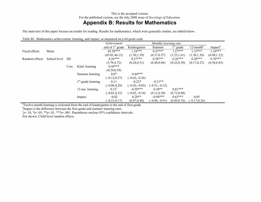
This is the accepted version. For the published version, see the July 2008 issue of Sociology of Education.
Appendix B: Results for Mathematics
The main text of this paper focuses on results for reading. Results for mathematics, which were generally similar, are tabled below.
Table B1. Mathematics achievement, learning, and impact, as measured on a 64-point scaleAchievement Monthly learning rate
end of 1st grade Kindergarten Summer 1st grade 12-montha Impactb
Fixed effects Mean 45.58***(45.01,46.15)
1.34***(1.30,1.39)
0.47***(0.37,0.57)
1.57***(1.53,1.61)
1.33***(1.30,1.36)
1.10***(0.98,1.22)
Random effects School level SD 4.26***(3.79,4.72)
0.27***(0.24,0.31)
0.58***(0.48,0.68)
0.26***(0.22,0.30)
0.20***(0.17,0.23)
0.70***(0.58,0.83)
Corr. Kind. learning 0.44***(0.29,0.59)
Summer learning 0.07(–0.12,0.27)
–0.44***(–0.62,–0.26)
1st-grade learning 0.11(–0.06,0.28)
–0.22*(–0.42,–0.03)
–0.31**(–0.51,–0.12)
12-mo. learning 0.15†
(–0.01,0.32)–0.50***
(–0.65,–0.34)0.30**
(0.11,0.50)0.81***
(0.73,0.88)Impact –0.02
(–0.21,0.17)0.28**
(0.07,0.48)–0.94***
(–0.96,–0.91)0.63***
(0.49,0.76)0.05
(–0.17,0.26)aTwelve-month learning is reckoned from the end of kindergarten to the end of first-grade.bImpact is the difference between the first-grade and summer learning rates.†p<.10, *p<.05, **p<.01, ***p<.001. Parentheses enclose 95% confidence intervals.Not shown: Child-level random effects.
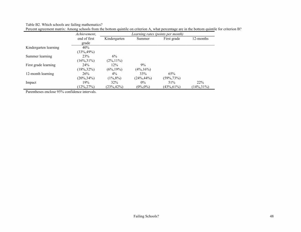
Failing Schools? 48
Table B2. Which schools are failing mathematics? Percent agreement matrix: Among schools from the bottom quintile on criterion A, what percentage are in the bottom quintile for criterion B?
Achievement, Learning rates (points per month)end of first
gradeKindergarten Summer First grade 12-months
Kindergarten learning 40%(33%,49%)
Summer learning 23%(16%,31%)
6%(2%,11%)
First grade learning 24%(18%,32%)
12%(6%,19%)
9%(4%,16%)
12-month learning 26%(20%,34%)
4%(1%,8%)
33%(24%,44%)
65%(59%,73%)
Impact 19%(12%,27%)
32%(23%,42%)
0%(0%,0%)
51%(43%,61%)
22%(14%,31%)
Parentheses enclose 95% confidence intervals.
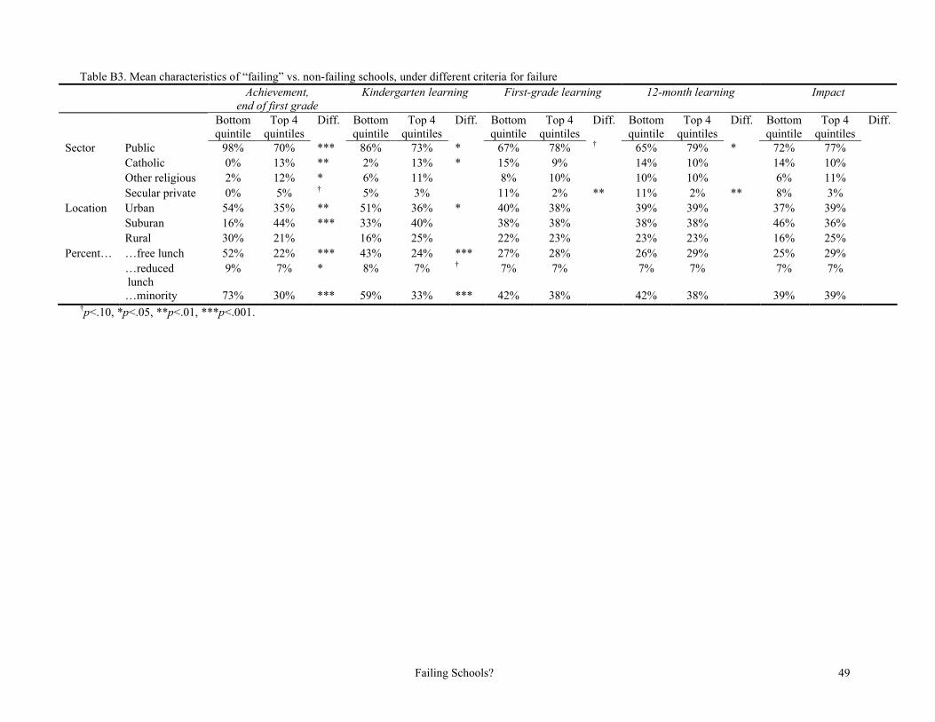
Failing Schools? 49
Table B3. Mean characteristics of “failing” vs. non-failing schools, under different criteria for failureAchievement,
end of first gradeKindergarten learning First-grade learning 12-month learning Impact
Bottomquintile
Top 4quintiles
Diff. Bottomquintile
Top 4quintiles
Diff. Bottomquintile
Top 4quintiles
Diff. Bottomquintile
Top 4quintiles
Diff. Bottomquintile
Top 4quintiles
Diff.
Sector Public 98% 70% *** 86% 73% * 67% 78% † 65% 79% * 72% 77%Catholic 0% 13% ** 2% 13% * 15% 9% 14% 10% 14% 10%Other religious 2% 12% * 6% 11% 8% 10% 10% 10% 6% 11%Secular private 0% 5% † 5% 3% 11% 2% ** 11% 2% ** 8% 3%
Location Urban 54% 35% ** 51% 36% * 40% 38% 39% 39% 37% 39%Suburan 16% 44% *** 33% 40% 38% 38% 38% 38% 46% 36%Rural 30% 21% 16% 25% 22% 23% 23% 23% 16% 25%
Percent… …free lunch 52% 22% *** 43% 24% *** 27% 28% 26% 29% 25% 29%…reduced lunch
9% 7% * 8% 7% † 7% 7% 7% 7% 7% 7%
…minority 73% 30% *** 59% 33% *** 42% 38% 42% 38% 39% 39%†p<.10, *p<.05, **p<.01, ***p<.001.
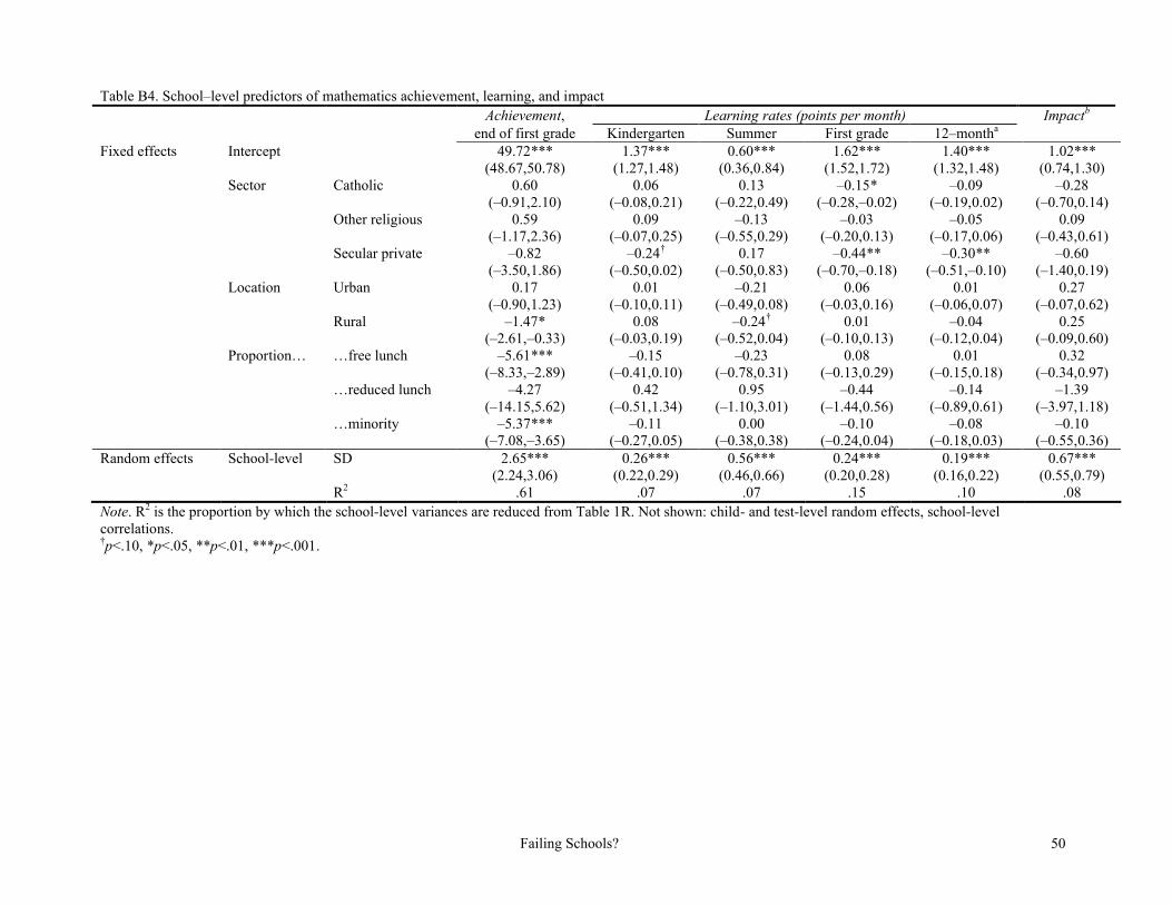
Failing Schools? 50
Table B4. School–level predictors of mathematics achievement, learning, and impact Achievement, Learning rates (points per month) Impactb
end of first grade Kindergarten Summer First grade 12–montha
Fixed effects Intercept 49.72***(48.67,50.78)
1.37***(1.27,1.48)
0.60***(0.36,0.84)
1.62***(1.52,1.72)
1.40***(1.32,1.48)
1.02***(0.74,1.30)
Sector Catholic 0.60(–0.91,2.10)
0.06(–0.08,0.21)
0.13(–0.22,0.49)
–0.15*(–0.28,–0.02)
–0.09(–0.19,0.02)
–0.28(–0.70,0.14)
Other religious 0.59(–1.17,2.36)
0.09(–0.07,0.25)
–0.13(–0.55,0.29)
–0.03(–0.20,0.13)
–0.05(–0.17,0.06)
0.09(–0.43,0.61)
Secular private –0.82(–3.50,1.86)
–0.24†
(–0.50,0.02)0.17
(–0.50,0.83)–0.44**
(–0.70,–0.18)–0.30**
(–0.51,–0.10)–0.60
(–1.40,0.19)Location Urban 0.17
(–0.90,1.23)0.01
(–0.10,0.11)–0.21
(–0.49,0.08)0.06
(–0.03,0.16)0.01
(–0.06,0.07)0.27
(–0.07,0.62)Rural –1.47*
(–2.61,–0.33)0.08
(–0.03,0.19)–0.24†
(–0.52,0.04)0.01
(–0.10,0.13)–0.04
(–0.12,0.04)0.25
(–0.09,0.60)Proportion… …free lunch –5.61***
(–8.33,–2.89)–0.15
(–0.41,0.10)–0.23
(–0.78,0.31)0.08
(–0.13,0.29)0.01
(–0.15,0.18)0.32
(–0.34,0.97)…reduced lunch –4.27
(–14.15,5.62)0.42
(–0.51,1.34)0.95
(–1.10,3.01)–0.44
(–1.44,0.56)–0.14
(–0.89,0.61)–1.39
(–3.97,1.18)…minority –5.37***
(–7.08,–3.65)–0.11
(–0.27,0.05)0.00
(–0.38,0.38)–0.10
(–0.24,0.04)–0.08
(–0.18,0.03)–0.10
(–0.55,0.36)Random effects School-level SD 2.65***
(2.24,3.06)0.26***
(0.22,0.29)0.56***
(0.46,0.66)0.24***
(0.20,0.28)0.19***
(0.16,0.22)0.67***
(0.55,0.79)R2 .61 .07 .07 .15 .10 .08
Note. R2 is the proportion by which the school-level variances are reduced from Table 1R. Not shown: child- and test-level random effects, school-level correlations.†p<.10, *p<.05, **p<.01, ***p<.001.
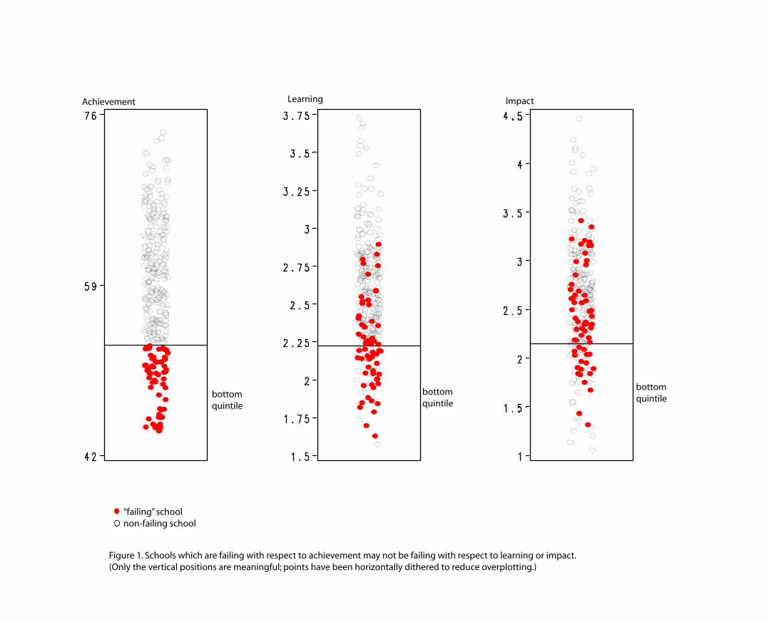
bottom quintile
bottom quintile
bottom quintile
LearningAchievement Impact
“failing” schoolnon-failing school
Figure 1. Schools which are failing with respect to achievement may not be failing with respect to learning or impact. (Only the vertical positions are meaningful; points have been horizontally dithered to reduce overplotting.)


![Failing Schools[1]](https://img.pdfslide.us/doc/110x75/577d2db41a28ab4e1eae1fd8/failing-schools1.jpg)