Are European sovereign bonds fairly priced? The role of modelling uncertainty

Journal of International Money and Finance 47 (2014) 239e267

Contents lists available at ScienceDirect

Journal of International Moneyand Finance

journal homepage: www.elsevier .com/locate/ j imf

Are European sovereign bonds fairly priced? Therole of modelling uncertainty*

Leo de Haan*, Jeroen Hessel, Jan Willem van den EndDe Nederlandsche Bank, Economics and Research Division, P.O. Box 98, 1000 AB Amsterdam,The Netherlands

JEL Classification:E43E44F34G15

Keywords:Sovereign bondInterest rateRisk premium

* The views expressed are those of the authorsymous referee, Jan Marc Berk, Christophe Blot, Jakoat DNB, participants of the 63rd conference of the MDebt Crises and Financial Stability (Toulon) and thMartin Admiraal, Ren�e Bierdrager, and Zion Gorgi* Corresponding author. Tel.: þ31 20 5243539; f

E-mail addresses: [email protected] (L. de Haan)

http://dx.doi.org/10.1016/j.jimonfin.2014.06.0010261-5606/© 2014 Elsevier Ltd. All rights reserved

a b s t r a c t

This paper examines the extent to which large swings of sovereignyields in euro area countries during the debt crisis can be attrib-uted to fundamentals, focusing on the inherent uncertainty inbond yield models. We show that the outcomes are stronglyaffected by modelling choices with regard to i) the confidencebands for the model prediction, ii) the assumption whether themodel coefficients are similar across countries or not, iii) thesample selection, iv) the inclusion of financial variables and v) thechoice of time-varying coefficients. These choices affect theexplanatory power of macro fundamentals and the extent ofmispricing.

© 2014 Elsevier Ltd. All rights reserved.

1. Introduction

Developments of bond yields are an issue for monetary policy as its effectiveness depends on thetransmission of money market rates into long-term bond yields (Cœur�e, 2012). Disorderly marketconditions can disturb this mechanism, if they go in tandem with excessive volatility in bond yields.Strong swings in bond yields may be due to (fair) changes in required compensation for credit risk,

and do not necessarily reflect official positions of DNB. We thank an anon-b de Haan, Alex Kostakis, Issouf Soumare, Peter van Els, seminar participantsidwest Finance Association (Orlando), the 2nd International Conference one 5th World Finance Conference (Venice) for useful comments and advice.provided data assistance.ax: þ31 20 5242526., [email protected] (J. Hessel), [email protected] (J.W. van den End).

.

mailto:[email protected]



http://crossmark.crossref.org/dialog/?doi=10.1016/j.jimonfin.2014.06.001&domain=pdf

www.sciencedirect.com/science/journal/02615606

www.elsevier.com/locate/jimf

http://dx.doi.org/10.1016/j.jimonfin.2014.06.001



L. de Haan et al. / Journal of International Money and Finance 47 (2014) 239e267240

market volatility and liquidity tensions. However, during periods of high market turmoil, bond yieldsmay also reflect risks associated with excessive risk aversion that is out of sync with economic fun-damentals and market conditions.

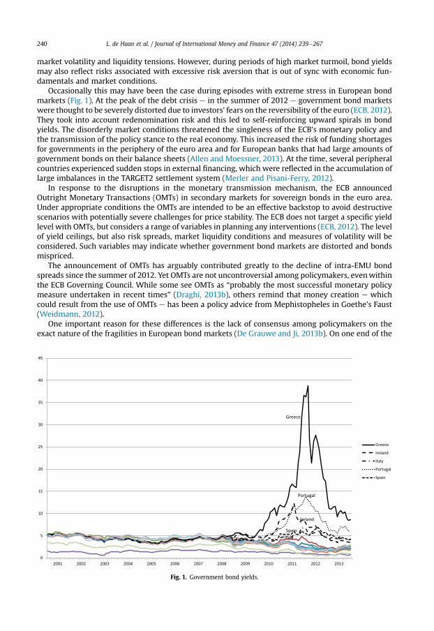
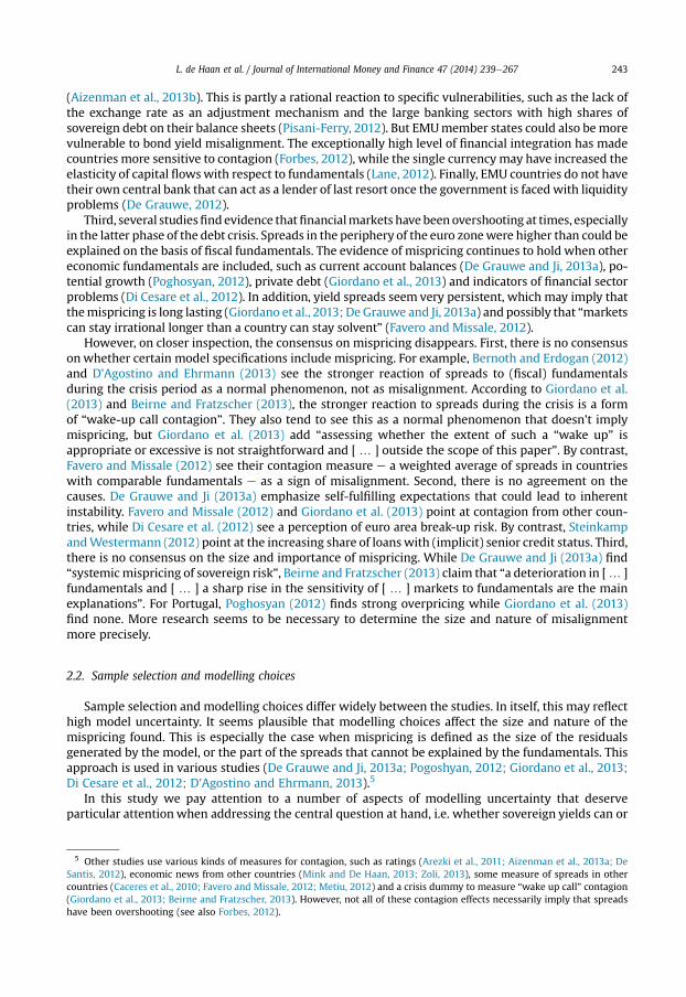
Occasionally this may have been the case during episodes with extreme stress in European bondmarkets (Fig. 1). At the peak of the debt crisis e in the summer of 2012 e government bond marketswere thought to be severely distorted due to investors' fears on the reversibility of the euro (ECB, 2012).They took into account redenomination risk and this led to self-reinforcing upward spirals in bondyields. The disorderly market conditions threatened the singleness of the ECB's monetary policy andthe transmission of the policy stance to the real economy. This increased the risk of funding shortagesfor governments in the periphery of the euro area and for European banks that had large amounts ofgovernment bonds on their balance sheets (Allen and Moessner, 2013). At the time, several peripheralcountries experienced sudden stops in external financing, which were reflected in the accumulation oflarge imbalances in the TARGET2 settlement system (Merler and Pisani-Ferry, 2012).

In response to the disruptions in the monetary transmission mechanism, the ECB announcedOutright Monetary Transactions (OMTs) in secondary markets for sovereign bonds in the euro area.Under appropriate conditions the OMTs are intended to be an effective backstop to avoid destructivescenarios with potentially severe challenges for price stability. The ECB does not target a specific yieldlevel with OMTs, but considers a range of variables in planning any interventions (ECB, 2012). The levelof yield ceilings, but also risk spreads, market liquidity conditions and measures of volatility will beconsidered. Such variables may indicate whether government bond markets are distorted and bondsmispriced.

The announcement of OMTs has arguably contributed greatly to the decline of intra-EMU bondspreads since the summer of 2012. Yet OMTs are not uncontroversial among policymakers, evenwithinthe ECB Governing Council. While some see OMTs as “probably the most successful monetary policymeasure undertaken in recent times” (Draghi, 2013b), others remind that money creation e whichcould result from the use of OMTs e has been a policy advice from Mephistopheles in Goethe's Faust(Weidmann, 2012).

One important reason for these differences is the lack of consensus among policymakers on theexact nature of the fragilities in European bond markets (De Grauwe and Ji, 2013b). On one end of the

Fig. 1. Government bond yields.

L. de Haan et al. / Journal of International Money and Finance 47 (2014) 239e267 241

spectrum, some see higher spreads as a rational reaction to increased insolvency risk due to deterio-rating fundamentals (e.g., Issing, 2009). In this vision, financial support via loans from the EFSF/ESM orvia ECB interventions carry large financial risks, while they also create moral hazard because thedisciplining effect of financial markets is reduced (Benink and Huizinga, 2013). On the other end of thespectrum, some argue that higher spreads result from overshooting financial markets, where fear andpanic can drive spreads away from fundamentals (e.g., De Grauwe and Ji, 2013a; Giavazzi et al., 2013).In this view, liquidity support is justified especially as self-fulfilling expectations could turn liquidityproblems into solvency problems (De Grauwe, 2012).

For policymakers, it is therefore very important to knowwhether and towhat extent sovereignyieldsof euro countries are misaligned compared to fundamentals. The answer to this question determineswhether market discipline can be relied on, or whether financial markets fail and support or in-terventions by the EFSF/ESM or ECB are needed. The answer is therefore not only relevant to assess the(future) policyof theECB, but it also influences the future institutionaldesignof EMU(Gilbert et al., 2013).

The research question of this paper is the extent to which the large swings of sovereign yields ofseveral euro area countries since 2010 can be attributed to fundamentals, given the inherent modeluncertainty. Yet a definite answer to the research question is not straightforward. Fundamental valuesof financial market variables are inherently uncertain. In addition, bond yields may react in a rationalway to political risks, such as government ineffectiveness in member states, indecisiveness at theEuropean level, political discussions about debt restructuring and private sector involvement, or openspeculation about the possibility of a euro-exit. Yet these aspects e including redenomination risks eare very difficult to quantify. Finally, recent research suggests that the reaction of bond yields tofundamentals is time-varying, due to fluctuations in global risk aversion (D'Agostino and Ehrmann,2013). This time variability has probably been even stronger in the euro area, where bond yieldshardly diverged between 1999 and 2008, but started to differ widely during the sovereign debt crisis.This unusual behavior of bond spreads poses important modelling challenges.

Rather than providing a final answer, we therefore emphasize the role of model uncertainty. Thisaspect is greatly underemphasized in the recently booming literature that explains bond yields frommacroeconomic fundamentals. We adopt the approach taken in this literature and estimate reducedform models for bond yields. This modelling choice is motivated by the question of whether bondyields are fairly priced with respect to macroeconomic fundamentals and market conditions. Thepurpose of this paper is to show the effect of model uncertainty when assessing whether sovereignbond yields are aligned with macroeconomic fundamentals. We do not aim at estimating the yieldcurve, so we refrain from estimating stochastic models, such as models that predict the yield curve oftomorrow by using today's observed yield data (see, for instance, Nelson and Siegel, 1987).1We are alsonot looking for the dynamics of impulse responses of bond yields to developments of fundamentalvariables, such as studies that use Vector Autoregressive models do (see Arezki et al., 2011). Finally, weare not looking for contagion or spill-over effects from one country to another, as e.g. Mink and DeHaan (2013) have done (see further Section 2).

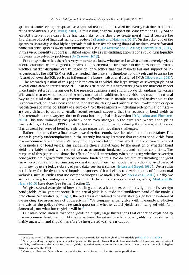
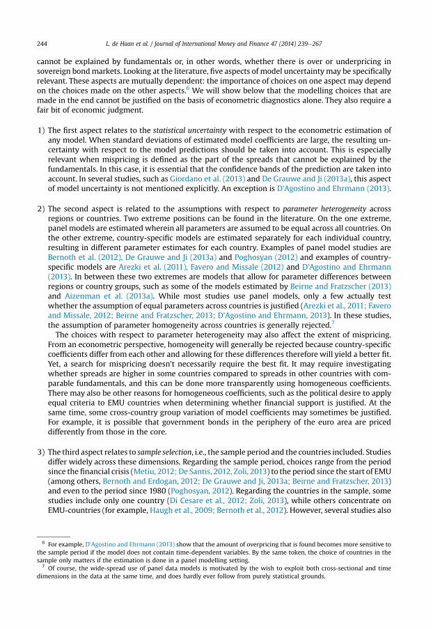
We give several examples of how modelling choices affect the extent of misalignment of sovereignbond yields. Misalignment occurs if the actual yield is outside the confidence band of the model'spredictions. Schematically, in Fig. 2, the red area is considered to be statistically significant evidence ofoverpricing, the green area of underpricing.2 We compare actual yields with in-sample predictionintervals, as the policy relevant research question is whether actual yields are misaligned with fun-damentals, not what future yields will be.3

Our main conclusion is that bond yields do display large fluctuations that cannot be explained bymacroeconomic fundamentals. At the same time, the extent to which bond yields are misaligned ishighly uncertain, and should therefore be interpreted with great caution.

1 A related strand of literature incorporates macroeconomic factors into yield curve models (H€ordahl et al., 2006).2 Strictly speaking, overpricing of an asset implies that the yield is lower than its fundamental level. However, for the sake of

simplicity and because this paper focuses on yields instead of asset prices, with ‘overpricing’ we mean that the yield is higherthan its fundamental level.

3 Ceteris paribus, confidence bands are wider for model forecasts than for model predictions.

time

95% confidence band

Predictedyield

Actualyield

%

= overpricing

= underpricing

Fig. 2. Overpricing and underpricing.


The remainder of this paper is structured as follows. Section 2 provides an overview of the empiricalliterature on sovereign bond yields and derives five major modelling choices. Section 3 presents ourbenchmark model and various alternative specifications, while Section 4 offers a description of thedata. Section 5 presents estimates of the benchmark model after which Section 6 shows how alter-native modelling choices affect the results. Section 7 concludes.

2. Literature review

This section first summarizes the main findings of the empirical literature on sovereign yields, afterwhich it focuses on the wide diversity in sample selection and modelling choices.

2.1. Main findings

There is an extensive and fastly growing body of empirical literature on sovereign yields. The Eu-ropean sovereign debt crisis has clearly increased the interest in this subject. Roughly three relevantfindings seem to emerge, even though there is no consensus.4

First, the reaction of financial markets is not constant over time. Spreads were exceptionally lowduring the first decade of EMU (Bernoth et al., 2012; Pogoshyan, 2012; Beirne and Fratzscher, 2013;D'Agostino and Ehrmann, 2013) and only started to increase after the start of the debt crisis. Thiswas partly due to an increase in global risk aversion (Haugh et al., 2009; Caceres et al., 2010; Aizenmanet al., 2013b), but spreads also reacted more strongly to fiscal fundamentals (Haugh et al., 2009; vonHagen et al., 2011; Bernoth et al., 2012; Bernoth and Erdogan, 2012; Giordano et al., 2013; Beirneand Fratzscher, 2013; D'Agostino and Ehrmann, 2013).

Second, EMU member states appear more vulnerable than countries having their own currencies.Spreads in the so-called ‘periphery’ of the euro area (Greece, Ireland, Italy, Portugal and Spain) arehigher than in countries with comparable fiscal fundamentals (De Grauwe and Ji, 2013a; Poghosyan,2012; D’Agostino and Ehrmann, 2013), even if emerging economies are included in the sample

4 Gilbert et al. (2013) provide a more elaborate overview of these three findings.


(Aizenman et al., 2013b). This is partly a rational reaction to specific vulnerabilities, such as the lack ofthe exchange rate as an adjustment mechanism and the large banking sectors with high shares ofsovereign debt on their balance sheets (Pisani-Ferry, 2012). But EMUmember states could also bemorevulnerable to bond yield misalignment. The exceptionally high level of financial integration has madecountries more sensitive to contagion (Forbes, 2012), while the single currency may have increased theelasticity of capital flowswith respect to fundamentals (Lane, 2012). Finally, EMU countries do not havetheir own central bank that can act as a lender of last resort once the government is faced with liquidityproblems (De Grauwe, 2012).

Third, several studiesfindevidence thatfinancialmarkets have beenovershooting at times, especiallyin the latter phase of the debt crisis. Spreads in the periphery of the euro zonewere higher than could beexplained on the basis of fiscal fundamentals. The evidence of mispricing continues to hold when othereconomic fundamentals are included, such as current account balances (De Grauwe and Ji, 2013a), po-tential growth (Poghosyan, 2012), private debt (Giordano et al., 2013) and indicators of financial sectorproblems (Di Cesare et al., 2012). In addition, yield spreads seem very persistent, which may imply thatthemispricing is long lasting (Giordano et al., 2013; De Grauwe and Ji, 2013a) and possibly that “marketscan stay irrational longer than a country can stay solvent” (Favero and Missale, 2012).

However, on closer inspection, the consensus on mispricing disappears. First, there is no consensusonwhether certain model specifications include mispricing. For example, Bernoth and Erdogan (2012)and D'Agostino and Ehrmann (2013) see the stronger reaction of spreads to (fiscal) fundamentalsduring the crisis period as a normal phenomenon, not as misalignment. According to Giordano et al.(2013) and Beirne and Fratzscher (2013), the stronger reaction to spreads during the crisis is a formof “wake-up call contagion”. They also tend to see this as a normal phenomenon that doesn't implymispricing, but Giordano et al. (2013) add “assessing whether the extent of such a “wake up” isappropriate or excessive is not straightforward and [ … ] outside the scope of this paper”. By contrast,Favero and Missale (2012) see their contagion measure e a weighted average of spreads in countrieswith comparable fundamentals e as a sign of misalignment. Second, there is no agreement on thecauses. De Grauwe and Ji (2013a) emphasize self-fulfilling expectations that could lead to inherentinstability. Favero and Missale (2012) and Giordano et al. (2013) point at contagion from other coun-tries, while Di Cesare et al. (2012) see a perception of euro area break-up risk. By contrast, SteinkampandWestermann (2012) point at the increasing share of loans with (implicit) senior credit status. Third,there is no consensus on the size and importance of mispricing. While De Grauwe and Ji (2013a) find“systemicmispricing of sovereign risk”, Beirne and Fratzscher (2013) claim that “a deterioration in [… ]fundamentals and [ … ] a sharp rise in the sensitivity of [ … ] markets to fundamentals are the mainexplanations”. For Portugal, Poghosyan (2012) finds strong overpricing while Giordano et al. (2013)find none. More research seems to be necessary to determine the size and nature of misalignmentmore precisely.

2.2. Sample selection and modelling choices

Sample selection and modelling choices differ widely between the studies. In itself, this may reflecthigh model uncertainty. It seems plausible that modelling choices affect the size and nature of themispricing found. This is especially the case when mispricing is defined as the size of the residualsgenerated by the model, or the part of the spreads that cannot be explained by the fundamentals. Thisapproach is used in various studies (De Grauwe and Ji, 2013a; Pogoshyan, 2012; Giordano et al., 2013;Di Cesare et al., 2012; D'Agostino and Ehrmann, 2013).5

In this study we pay attention to a number of aspects of modelling uncertainty that deserveparticular attentionwhen addressing the central question at hand, i.e. whether sovereign yields can or

5 Other studies use various kinds of measures for contagion, such as ratings (Arezki et al., 2011; Aizenman et al., 2013a; DeSantis, 2012), economic news from other countries (Mink and De Haan, 2013; Zoli, 2013), some measure of spreads in othercountries (Caceres et al., 2010; Favero and Missale, 2012; Metiu, 2012) and a crisis dummy to measure “wake up call” contagion(Giordano et al., 2013; Beirne and Fratzscher, 2013). However, not all of these contagion effects necessarily imply that spreadshave been overshooting (see also Forbes, 2012).


cannot be explained by fundamentals or, in other words, whether there is over or underpricing insovereign bondmarkets. Looking at the literature, five aspects of model uncertainty may be specificallyrelevant. These aspects are mutually dependent: the importance of choices on one aspect may dependon the choices made on the other aspects.6 We will show below that the modelling choices that aremade in the end cannot be justified on the basis of econometric diagnostics alone. They also require afair bit of economic judgment.

1) The first aspect relates to the statistical uncertainty with respect to the econometric estimation ofany model. When standard deviations of estimated model coefficients are large, the resulting un-certainty with respect to the model predictions should be taken into account. This is especiallyrelevant when mispricing is defined as the part of the spreads that cannot be explained by thefundamentals. In this case, it is essential that the confidence bands of the prediction are taken intoaccount. In several studies, such as Giordano et al. (2013) and De Grauwe and Ji (2013a), this aspectof model uncertainty is not mentioned explicitly. An exception is D'Agostino and Ehrmann (2013).

2) The second aspect is related to the assumptions with respect to parameter heterogeneity acrossregions or countries. Two extreme positions can be found in the literature. On the one extreme,panel models are estimated wherein all parameters are assumed to be equal across all countries. Onthe other extreme, country-specific models are estimated separately for each individual country,resulting in different parameter estimates for each country. Examples of panel model studies areBernoth et al. (2012), De Grauwe and Ji (2013a) and Poghosyan (2012) and examples of country-specific models are Arezki et al. (2011), Favero and Missale (2012) and D'Agostino and Ehrmann(2013). In between these two extremes are models that allow for parameter differences betweenregions or country groups, such as some of the models estimated by Beirne and Fratzscher (2013)and Aizenman et al. (2013a). While most studies use panel models, only a few actually testwhether the assumption of equal parameters across countries is justified (Arezki et al., 2011; Faveroand Missale, 2012; Beirne and Fratzscher, 2013; D'Agostino and Ehrmann, 2013). In these studies,the assumption of parameter homogeneity across countries is generally rejected.7

The choices with respect to parameter heterogeneity may also affect the extent of mispricing.From an econometric perspective, homogeneity will generally be rejected because country-specificcoefficients differ from each other and allowing for these differences therefore will yield a better fit.Yet, a search for mispricing doesn't necessarily require the best fit. It may require investigatingwhether spreads are higher in some countries compared to spreads in other countries with com-parable fundamentals, and this can be done more transparently using homogeneous coefficients.There may also be other reasons for homogeneous coefficients, such as the political desire to applyequal criteria to EMU countries when determining whether financial support is justified. At thesame time, some cross-country group variation of model coefficients may sometimes be justified.For example, it is possible that government bonds in the periphery of the euro area are priceddifferently from those in the core.

3) The third aspect relates to sample selection, i.e., the sample period and the countries included. Studiesdiffer widely across these dimensions. Regarding the sample period, choices range from the periodsince the financial crisis (Metiu, 2012; De Santis, 2012, Zoli, 2013) to the period since the start of EMU(among others, Bernoth and Erdogan, 2012; De Grauwe and Ji, 2013a; Beirne and Fratzscher, 2013)and even to the period since 1980 (Poghosyan, 2012). Regarding the countries in the sample, somestudies include only one country (Di Cesare et al., 2012; Zoli, 2013), while others concentrate onEMU-countries (for example, Haugh et al., 2009; Bernoth et al., 2012). However, several studies also

6 For example, D'Agostino and Ehrmann (2013) show that the amount of overpricing that is found becomes more sensitive tothe sample period if the model does not contain time-dependent variables. By the same token, the choice of countries in thesample only matters if the estimation is done in a panel modelling setting.

7 Of course, the wide-spread use of panel data models is motivated by the wish to exploit both cross-sectional and timedimensions in the data at the same time, and does hardly ever follow from purely statistical grounds.


include countries from outside the euro area, such as EU-countries (Aizenman et al., 2013a), otheradvanced economies (De Grauwe and Ji, 2013a; Poghosyan, 2012; D'Agostino and Ehrmann, 2013)and emergingmarkets (Aizenman et al., 2013b; Beirne and Fratzscher, 2013; Aizenman et al., 2013a).Sample selection may affect the extent of mispricing found, because the econometric estimation

methodsmaximize the fit of themodel over the sample period (D'Agostino and Ehrmann, 2013) and(in case of a panel) the countries included in the sample. To determine possible misalignment, it istherefore important that yields in the sample aremore or less “normal” on average. This normality isdifficult to identify, given the time variation in the spreads and the cross-country differences. Forexample, estimation over the crisis period might be biased because spreads were relatively highduring that period. On the other hand, estimation over the EMU-period might be influenced by theexceptionally low intra-EMU spreads before the crisis. In fact, the few studies that acknowledge thatintra-EMU spreads were too low in the pre-crisis period include either data from before the start ofEMU (Bernoth et al., 2012; D'Agostino and Ehrmann, 2013), countries outside EMU (Beirne andFratzscher, 2013) or both (Poghosyan, 2012).

4) The fourth aspect is related to the incorporation of financial market indicators in the model. Manystudies include financial market indicators to account for market conditions affecting sovereignyields. The choice of financial market variables varies considerably, but two groups of variables canbe distinguished. One group represents changes in global risk aversion. Usually one such globalvariable is included into the model, which ranges from the VIX index (see, for example, Giordanoet al., 2013; Beirne and Fratzscher, 2013; Aizenman et al., 2013a; D'Agostino and Ehrmann, 2013),to US corporate bond spreads (Haugh et al., 2009; Favero and Missale, 2012; Bernoth and Erdogan,2012), and the TED spread (Aizenman et al., 2013b). Another group of financial market variablesaims at representing more structural characteristics of the bond markets of individual countries, interms of market depth and liquidity. Usually a country-specific variable is included, which variesfrom an indicator of market size (Haugh et al., 2009; Bernoth et al., 2012; D'Agostino and Ehrmann,2013) to bid-ask spreads (Bernoth and Erdogan, 2012; Giordano et al., 2013).The inclusion of financial market variables in a model for sovereign yields could also affect the

extent of mispricing found. Financial market variables allow yield spreads to display variation overtime (global risk aversion) and across countries (liquidity) that is not explained by macroeconomicfundamentals alone. To some extent this seems to be justified, since these financial market variablesreflect volatility and liquidity risks that are and should be priced in the market. On the other hand,market sentiments may be overly optimistic or pessimistic and therefore the cause of under oroverpricing. Several observers claim that global risk aversion was too low before the crisis, while itmay have been too high during the most intense phase of the crisis (e.g., Knot and Verkaart, 2013).Likewise, bid-ask spreads could be affected when sovereign yields are under pressure.

5) The final modelling choice is how to deal with the apparent time variability in the reaction of yieldspreads. Many studies allow for some form of time variability of the parameters. Some even allowthe coefficients to change continuously over a certain horizon (D'Agostino and Ehrmann, 2013;Bernoth and Erdogan, 2012). Other studies assume coefficients to remain constant throughoutthe whole sample period (Poghosyan, 2012; Steinkamp and Westermann, 2012). In between thesetwo extremes are studies allowing for a structural break in several coefficients, for example, due tothe financial crisis or the sovereign debt crisis (e.g., Bernoth et al., 2012; Giordano et al., 2013; Beirneand Fratzscher, 2013). Others allow for non-linearities by interacting some variables with risk in-dicators (Haugh et al., 2009) or adding squared terms of fiscal fundamentals (Bernoth et al., 2012;De Grauwe and Ji, 2013a; Di Cesare et al., 2012). Finally, some studies deal with time variability byincorporating some kind of contagion measure, such as spreads in other countries (Favero andMissale, 2012) or credit ratings (Arezki et al., 2011; Aizenman et al., 2013a).The extent of mispricing found will also depend on whether and how time-variability is incor-

porated. The inclusion of time-variability allows for higher coefficients in the period of the sover-eign debt crisis, which implies that a larger part of the yield spreads is explained bymacroeconomicfundamentals. The specificmethod of time-variability also seems tomatter.While the incorporation


of a crisis dummy only allows coefficients to differ between the crisis and the pre-crisis period, theincorporation of time-varying coefficients allows for some variation within the crisis period. Thismay be justified to some extent, as the severity of the crisis also varies, for instance, due to politicaldevelopments. However, too much time variation in the coefficients increases the chance that allyield developments are attributed to fundamentals. There clearly is a trade-off here, which may behard to determine exactly.

Our contribution is that we show how the above-mentioned aspects of modelling uncertainty affectthe extent of mispricing found.

3. The benchmark model and some variants

In this section, we first present our benchmark model, and subsequently several alternative spec-ifications that represent modelling uncertainty.

3.1. The benchmark model

Based on the preferred habitat theory of the yield curve (Modigliani and Shiller, 1973), we assumethat sovereign yields (rit) consist of three components: a risk-free component (rfit), a risk premium (rpit)and a residual term (eit):

rit ¼ rfit þ rpit þ eit (1)

where i denotes the country and t the time period. The risk premium not only compensates for inflationand credit risks, but also for volatility and liquidity risks. The first two risk factors are determined byexpectations with respect to the macro-economic fundamentals of a country, the last two by acountry's financial market conditions, i.e. liquidity and volatility, for which investors require a riskpremium.

The macro-economic fundamentals, reflecting a country's earning capacity and credit worthiness,include real gdp growth (gdp), inflation (cpi), the government debt ratio (debt) and the current accountratio (car). These variables are used in most models that explain sovereign bond yields from macro-economic fundamentals (see Section 2).When available, we use expectations of market participants forthese macro-economic fundamentals (Consensus forecasts), because expectations affect market ratesin the first place.8 Consensus forecasts are forward looking and contain new information in addition torealizations. Ager et al. (2009) and Dovern and Weisser (2011), for example, find empirical evidencethat Consensus forecasts are different from realizations especially during periods of pronouncedmacroeconomic shocks and in situations where forecasters have to learn about large structural shocks.These expectations are relevant for our model, as they may well be another source of market fluctu-ations. Our sample period, in which a sovereign debt crisis emerged, is typically a period of suchstructural shocks. By using Consensus forecasts we follow D'Agostino and Ehrmann (2013), who werethe first to use such data for the modelling of sovereign yields; they do this for the G7 countries. Theadvantages of the Consensus forecasts are that, unlike official public forecasts, they have a monthlyfrequency and reflect the predictions of financial market participants.

For the financial market conditions we use a latent variable (fin), capturing volatility and liquidity ofgovernment bond markets in individual countries. These factors partly determine the efficiency of thepricing process and thereby the extent to which yields fairly reflect macroeconomic fundamentals. Wealso interact the financial market conditions variable with government debt (debt x fin), assuming thatwhen financial markets are nervous, market participants are more alert with respect to the countries'credit worthiness than they are under normal market conditions (see, for instance, Haugh et al., 2009).

8 Following D'Agostino and Ehrmann (2013), we use the debt ratio as explanatory variable and not the government deficit.For our sample including smaller countries, Consensus forecast data for the latter variable are not always available.


In other words, we assume that any non-linearity in the relation between credit worthiness andsovereign yields may be driven by market conditions. The benchmark model reads:

rit ¼ a0i þ a1rfit þ a2cpiit þ a3gdpit þ a4debtit þ a5debtit � finit þ a6carit þ a7finit þ eit (2)

Our priors are: a1, a2, a4, a5, a7 � 0 and a3, a6 � 0. We do not restrict a1 to be equal to 1, as our proxyfor the risk-free rate is the swap rate for the euro areawith a maturity of 2 years (10 year maturities arenot available). Therefore, the proxy is an imperfect measure for the risk-free rate and the coefficient isexpected to be close to but not necessarily equal to 1.

The residual (eit) reflects the effect of market sentiments unrelated tomacro-economic and financialmarket conditions, as in, for example, De Grauwe and Ji (2013a), Pogoshyan (2012) and D'Agostino andEhrmann (2013). Market sentiments can be excessively pessimistic or optimistic and generate over orunderpricing of the interest rate, respectively.

In order to assess whether misalignment of yields has occurred during the crisis, we estimate model(2) and compare themodel predictions with actual bond rates, taking into account the predictions' 95%confidence bands.

3.2. Alternative specifications

We also use several alternative specifications and propose an alternative sample selection. Our aimis to show how thesemodelling uncertainties may affect the extent of misalignment of bond yields. Weconsider the five sources of model uncertainty which have been discussed in Section 2.2.

Model uncertainty 1. The use and calculation of confidence bands for the model prediction is a sourceof model uncertainty.

The search for over or underpricing of sovereign yields essentially implies looking for an omittedvariable bias in the regression results. In the present case, the omitted variable could be irrationalmarket optimism or pessimism, which is typically hard to measure. Contagion could be such a variabletoo. Omission of such variables may result in the residuals being consecutively positive or negative,respectively, depending on whether there is excessive pessimism or optimism in the sovereign bondmarket. Hence, when there is over or underpricing, by definition, there should be positive or negativeautocorrelation of the residuals. OLS estimates for model coefficients in the presence of autocorrelationare unbiased. However, they no longer have the minimum variance property, making confidence in-tervals and hypothesis tests based on t and F distributions unreliable. Computed variances and stan-dard errors of forecasts may be inaccurate when autocorrelation is not accounted for. Therefore, wereport standard errors which are robust to clustering, autocorrelation and heteroskedasticity.9

In order to show the effect of neglecting the effect of autocorrelation on the standard errors, we alsocalculate prediction confidence bands using non-robust (OLS) standard errors.

Model uncertainty 2. The choice of common versus country-specific coefficients is a source of modeluncertainty.

Model (2), our benchmark model, is a fixed effects panel model. The intercept a0i is country specific;the latter represent the so-called ‘fixed effects’ allowing for time-invariant differences in interest ratesbetween countries. The coefficients of the explanatory variables are assumed to be equal acrosscountries, as are their marginal effects. Our assumption behind this modelling framework is that in-vestors assess country risks in a portfolio context and use similar norms towards the issuing countries,like rating agencies do (as discussed in Section 2.2). Because the pooling assumption is strong, we also

9 Using standard notation, the OLS variance estimator is VarOLS ¼ 1N�k

PNi¼1e

2i ,ðX0XÞ�1, whereas the robust cluster variance

estimator is Varcluster ¼ ðX0XÞ�1$Pnc

j¼1u0juj$ðX0XÞ�1; where uj ¼

P

jclustereixi and nc is the total number of clusters, ei is the residual

for the ith observation and xi is a row vector of predictors including the constant. For simplicity, the multiplier (which is close to1) has been omitted for the formula for Varcluster. For more information on robust standard errors in panel regressions, see e.g.Hoechle (2007).


test heterogeneity of some of the coefficients across regions or country groups (as in Beirne andFratzscher, 2013), using a region or country group dummy Dg:

rit ¼ a0i þ a1rfit þ a2cpiit þ a3cpiit$Dg þ a4gdpit þ a5gdpit$Dg þ a6debtit þ a7debtit$Dg

þ a8debtit � finit þ a9debtit � finit$Dg þ a10carit þ a11carit$Dg þ a12finit þ a13finit$Dg þ eit(3)

We also estimatemodels separately for each country, thus allowing all coefficients to differ betweenall countries (as in, for instance, D'Agostino and Ehrmann, 2013):

rit ¼ a0i þ a1irfit þ a2icpiit þ a3igdpit þ a4idebtit þ a5idebtit � finit þ a6icarit þ a7ifinit þ eit(4)

The main advantage of panel data models is that both time and cross-sectional information in thedata are exploited. Another important advantage of panel data models as opposed to country-specificmodels, which is specifically relevant for the research question at hand, is that the residuals do not haveto add up to zero for each country. In other words, while country-specific models force overpricing andunderpricing for a country to cancel out, panel data models allow countries to exhibit more overpricingthan underpricing or vice versa during the sample period.

Model uncertainty 3. The sample selection is a source of model uncertainty.As the selection of countries is important, we select a representative group of 17 advanced econ-

omies. Not only 11 euro area countries, but also 6 non-euro area countries are selected. The latter groupconsists of both EU and non-EU countries. More information follows in the Data Section. For our sampleperiod (January 2001eDecember 2013) we have datawith a relatively high (monthly) frequency whichallows us to capture the developments in financial markets. To show the effects of sample selection onthe findings, we estimate our models for the whole sample and for sub-samples.

Model uncertainty 4. The choice of including or excluding financial market variables is a source ofmodel uncertainty.

In our benchmark model, financial market conditions (fin) are included. The reason is that ourtheoretical model assumes that the risk premium also contains a premium for market volatility andliquidity. One could question whether this is justified. Often, in times of stress on financial markets,liquidity is extremely low and volatility high, so that implicitly part of the mispricing is added as anexplanatory variable. Therefore, we also estimate the fixed effects panel model excluding fin anddebt � fin among the explanatory variables (as in De Grauwe and Ji, 2013a; Poghosyan, 2012):

rit ¼ a0i þ a1rfit þ a2cpiit þ a3gdpit þ a4debtit þ a5carit þ eit (5)

Model uncertainty 5. The choice of fixed versus time-varying coefficients is a source of modeluncertainty

In benchmark model (2), the coefficients are fixed throughout the whole sample period, as inPoghosyan (2012) and Steinkamp and Westermann (2012). However, it is conceivable that the rela-tionship is not constant through time. Hence, following, for instance, Bernoth et al. (2012), Giordanoet al. (2013) and Beirne and Fratzscher (2013), we also estimate the model interacting with adummy variable Dc distinguishing the crisis period from the pre-crisis period, which is set to start fromJanuary 2010 onwards.

rit ¼ a0i þ a1rfit þ a2cpiit þ a3cpiit$Dc þ a4gdpit þ a5gdpit$Dc þ a6debtit þ a7debtit$Dc

þ a8debtit � finit þ a9debtit � finit$Dc þ a10carit þ a11carit$Dc þ a12finit þ a13finit$Dc þ eit(6)


In the empirical section, we will illustrate how these sources of model uncertainty affect the extentof over and underpricing. But first, we discuss the data.

4. Data

Our dataset contains 17 advanced economies, of which 11 euro countries and 6 non-euro countries(for comparison purposes).10 The data frequency is monthly and the sample period is January 2001 toDecember 2013. The panel data set is highly balanced. Hence, we extend the sample of D'Agostino andEhrmann (2013), who also use Consensus forecasts, from their G7 countries to our 17 countries.We add6 non-euro countries where the bulk of the literature only includes euro countries.11 Focusing onadvanced economies only seems appropriate as the sovereign debt crisis hit the euro area and thewestern world.

The dependent variable is the 10 year sovereign bond yield (r). For the risk-free rate (rf) we use theswap rate (euro overnight index for euro area countries; US and UK swap rates for the US and the UK,respectively).

For the macroeconomic variables we use Consensus forecasts, which are available for eachmonth m of a particular year for the current year y and the next year y þ 1. Following Dovern et al.(2012) and D'Agostino and Ehrmann (2013), we derive average forecasts for the coming 12 months.This acknowledges that interest rates reflect market expectations about future developments. If Fymis the Consensus forecast in month m for the current year y, and Fyþ1

m is the Consensus forecast fory þ 1, then the weighted average for the next 12 months is defined as:Fym,ð12�mÞþFyþ1

m ,m12 ; withm ¼ 1; :::;12.

The market conditions variable is the principal factor of two financial variables: volatility andliquidity. Liquidity is measured as the monthly average of daily bid-ask spreads, volatility is themonthly average of the daily differences between the highest and lowest bond price. We take theprincipal factor of these two highly correlated variables (within correlation is 0.80) to reduce thenumber of explanatory variables in our regression models and to have one composite indicator offinancial market conditions reflecting both liquidity and volatility.

Appendix A gives the definitions and sources of all variables. Table 1 presents summary statistics.Table 2 reports the correlation matrix for the panel-demeaned variables, i.e. the variables minus themeans by country. The reason for showing correlations for panel-demeaned variables is that the panelmodels assume fixed country effects, so that the relevant variables to look at are the variables afterremoving the panel means. Most right-hand side variables are not strongly correlated (correlations arebelow 0.45), with a few exceptions. We will test whether multicollinearity is a problem for ourbenchmark regression model.

The outcomes of a unit root test suggested by Levin et al. (2002) show that, when suppressingpanel-specific means, the presence of a unit root in all panels can be rejected for all variables except carand debt (Appendix B).

5. Results for the benchmark model

The results of the benchmark model (2) are presented in the first column of Table 3. The (robust)standard errors indicate that rf, gdp and debt are statistically significant and their coefficients have theexpected signs. The other variables, cpi, fin x debt, fin and car are not significant.12 Ourmeasure fin is notused in the rest of the literature, which makes it difficult to compare results. The insignificance of car isalso found by De Grauwe and Ji (2013a) and Beirne and Fratzscher (2013), while D'Agostino and

10 The 11 euro countries are Austria, Belgium, Germany, Finland, France, Greece, Ireland, Italy, the Netherlands, Portugal andSpain. The 6 non-euro countries are Canada, Japan, Sweden, Switzerland, the United Kingdom and the United States.11 To compare, De Grauwe en Yi (2012) have EMU-countries plus 8 other advanced economies. True, Poghosyan (2012) has 22advanced economies; however, he uses annual instead of monthly data and realisations instead of expectations. Other studiesincluding more countries typically include emerging economies.12 Multicollinearity does not seem to be a problem; the highest value for the Variance Inflation Factor is 5.1.

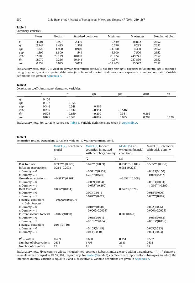
Table 2Correlation coefficients, panel demeaned variables.

r rf cpi gdp debt fin

rf 0.106cpi 0.167 0.354gdp �0.344 0.548 0.565debt 0.286 �0.632 �0.351 �0.546fin 0.525 �0.159 �0.209 �0.361 0.362car 0.025 �0.061 �0.097 0.055 0.209 0.120

Explanatory note. For variable names, see Table 1. Variable definitions are given in Appendix A.

Table 1Summary statistics.

Mean Median Standard deviation Minimum Maximum Number of obs.

r 4.001 3.997 2.419 0.439 38.832 2652rf 2.347 2.425 1.561 0.076 6.283 2652cpi 1.823 1.900 0.900 �1.300 4.400 2652gdp 1.599 1.800 1.544 �5.300 7.500 2652debt 82.888 73.129 40.078 26.024 249.741 2652fin 2.070 �0.226 20.841 �0.671 227.850 2652car 0.554 0.095 5.071 �14.203 15.522 2652

Explanatory note. Yield 10 ¼ yield on 10 year government bond, rf ¼ risk free rate, cpi ¼ expected inflation rate, gdp ¼ expectedreal gdp growth, debt ¼ expected debt ratio, fin ¼ financial market conditions, car ¼ expected current account ratio. Variabledefinitions are given in Appendix A.

Table 3Estimation results. Dependent variable is yield on 10 year government bond.

Model (2), Benchmarkmodel

Model (3) for eurocountries, interactedwith periphery dummy

Model (5), i.e.excluding financialconditions

Model (6), interactedwith crisis dummy

(1) (2) (3) (4)

Risk free rate 0.717*** (0.129) 0.622** (0.099) 0.831*** (0.187) 0.595*** (0.130)Inflation expectations 0.214 (0.293) 0.081 (0.223)x Dummy ¼ 0 �0.371**(0.132) �0.115(0.150)x Dummy ¼ 1 1.297**(0.566) �0.069(0.247)Growth expectations �0.513**(0.261) �0.653**(0.308)x Dummy ¼ 0 �0.059(0.064) �0.153(0.093)x Dummy ¼ 1 �0.675**(0.260) �1.210***(0.390)Debt forecast 0.036**(0.014) 0.049**(0.020)x Dummy ¼ 0 0.003(0.011) 0.018*(0.009)x Dummy ¼ 1 0.078***(0.022) 0.002**(0.007)Financial conditions� Debt forecast

�0.00006(0.0007)

x Dummy ¼ 0 0.010***(0.002) 0.002(0.006)x Dummy ¼ 1 �0.0005(0.0003) 0.0001(0.0005)Current account forecast �0.025(0.050) 0.006(0.043)x Dummy ¼ 0 �0.035(0.031) �0.035(0.053)x Dummy ¼ 1 �0.161***(0.048) �0.135*(0.076)Financial conditions 0.051(0.130)x Dummy ¼ 0 �0.105(0.149) 0.063(0.283)x Dummy ¼ 1 0.043(0.060) 0.003(0.094)

R2 e within 0.469 0.600 0.351 0.567Number of observations 2633 1708 2633 2633Number of countries 17 11 17 17

Explanatory note. Fixed country effects included (not reported). Robust standard errors within parentheses. ***, **, * denote p-values less than or equal to 1%, 5%, 10%, respectively. Formodel (3) and (6), coefficients are reported for subsamples for which theinteracted dummy variable is equal to 0 and 1, respectively. Variable definitions are given in Appendix A.



Ehrmann (2013) do find significant results. Our variable cpi is not used in many studies, but Poghosyan(2012) finds a significant effect.

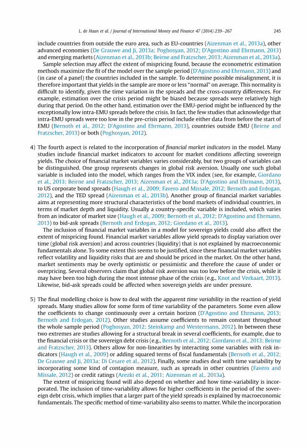
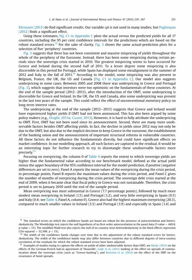
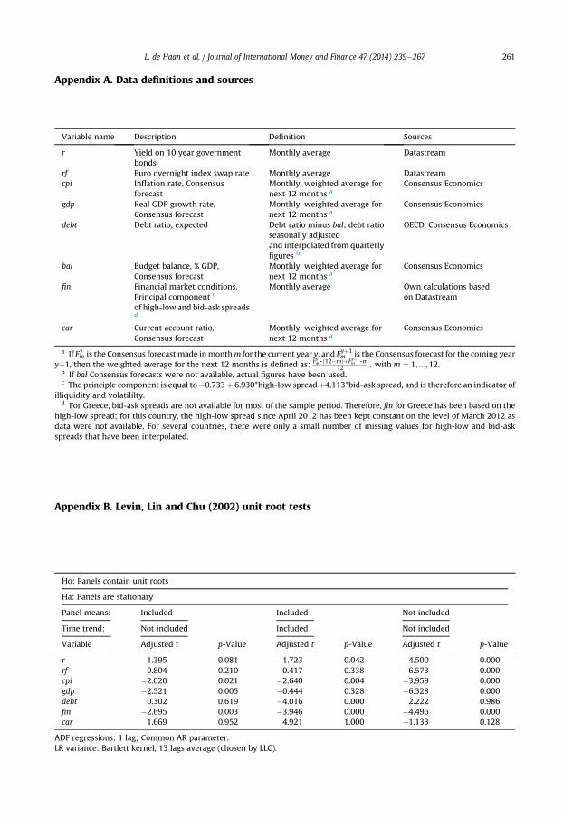
Using these estimates, Fig. C1 in Appendix C plots the actual versus the predicted yields for all 17countries, including the 95 per cent confidence intervals for the predictions which are based on therobust standard errors.13 For the sake of clarity, Fig. 3 shows the same actual-prediction plots for aselection of five ‘periphery’ countries.

Fig. 3 suggests that there has not been consistent and massive mispricing of yields throughout thewhole of the periphery of the Eurozone. Instead, there has been some mispricing during certain pe-riods since the sovereign crisis started in 2010. The greatest mispricing seems to have occurred forGreece and Ireland during the second half of 2011. To a lesser degree some mispricing is alsodiscernible in this period for Portugal, while Spain has displayed some misalignment in the summer of2012 and Italy in the fall of 2011.14 According to the model, some mispricing was also present inBelgium, France, the UK, the US and Canada (Fig. C1 in Appendix C). Our model also suggestsunderpricing in some cases. Between 2005 and 2008 there was underpricing in Greece and Portugal(Fig. 3), which suggests that investors were too optimistic on the fundamentals of these countries. Atthe end of the sample period (2012e2013), after the introduction of the OMT, some underpricing isdiscernible for Greece and Ireland. In the UK, the US and Canada, also some underpricing was presentin the last two years of the sample. This could reflect the effect of unconventional monetary policy onlong-term interest rates.

The underpricing at the end of the sample (2012e2013) suggests that Greece and Ireland wouldhave experienced higher yields if OMT had not been announced. This has also been argued by somepolicy makers (e.g., Draghi, 2013a; Cœur�e, 2013). However, it is hard to fully attribute the underpricingto OMT. First, OMT has not been used since its announcement. Second, there are many more unob-servable factors besides OMT affecting yields. In fact, the decline in yields since 2012 may not only bedue to the OMT, but also due to the implicit decision to keep Greece in the eurozone, the establishmentof the banking union and the announcement of important structural reforms in vulnerable countries.All these factors do not influence the fundamentals directly, but could have significant effects onmarket confidence. In our modelling approach, all such factors are captured in the residual. It would bean interesting topic for further research to try to disentangle these unobservable factors moreprecisely.15

Focusing on overpricing, the column 0 of Table 4 reports the extent to which sovereign yields arehigher than the fundamental value according to our benchmark model, defined as the actual yieldminus the upper boundary of the 95% confidence interval for themodel prediction, if positive (negativedifferences are set to zero). Panel A reports the mean values of the overpricing during the crisis period,in percentage points, Panel B reports the maximum values during the crisis period, and Panel C givesthe number of months of overpricing during the crisis period. The sovereign debt crisis started at theend of 2009, when it became clear that fiscal policy in Greece was not sustainable. Therefore, the crisisperiod is set to January 2010 until the end of the sample period.

Mean overpricing was most substantial in Greece (7.7 percentage points), followed by much moremodest mean overpricing in Ireland (1.5) and Portugal (1.2), and very little overpricing in Spain (0.5)and Italy (0.4; see Table 4, Panel A, column 0). Greece also had the highest maximum overpricing (20.3),compared to much smaller values in Ireland (3.5) and Portugal (3.9) and especially in Spain (1.4) and

13 The standard errors on which the confidence bands are based are robust for the presence of autocorrelation and hetero-skedasticity. The Wooldridge test rejects the null hypothesis of no first-order autocorrelation in the panel data (F-value ¼ 449.8,p-value < 1%). The modified Wald test also rejects the null of no country-wise heteroskedasticity in the fixed effects regression(Chi-squared ¼ 32,398; p < 1%).14 The width of the confidence bands changes over time due to the adjustment of the robust standard errors for hetero-skedasticity. The width of the confidence bands may also differ between countries due to different degrees of intra-countrycorrelation of the residuals for which the robust standard errors have been adjusted.15 Examples of studies trying to capture the effects on yields of other unobservable factors than OMT, are Mody (2014) on theeffects of the German-French bail-in agreement of ‘Deauville’, Gade et al. (2013) looking at the effect on spreads of commu-nication about the sovereign crisis (such as “Greece-bashing”), and Beetsma et al. (2014) on the effect of the SMP on thecovariance of bond spreads.

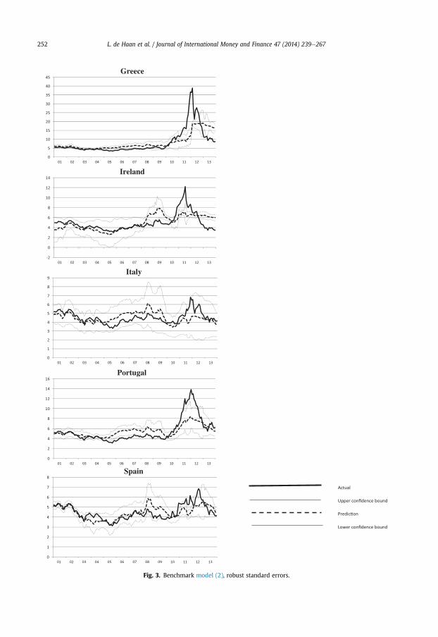
Fig. 3. Benchmark model (2), robust standard errors.


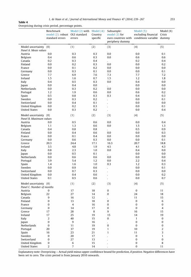
Table 4Overpricing during crisis period, percentage points.

Benchmarkmodel (2): robuststandard errors

Model (2) withOLS standarderrors

Model (4):Countryspecific

Subsample:model (3) foreuro countries withperiphery dummy

Model (5):excluding financialconditions variable

Model (6)Crisisdummy

Model uncertainty (0) (1) (2) (3) (4) (5)Panel A. Mean valuesAustria 0.0 0.3 0.3 0.0 0.0 0.1Belgium 0.4 0.6 0.3 0.0 0.6 0.6Canada 0.2 0.3 0.4 . 0.2 0.4Finland 0.0 0.2 0.3 0.0 0.0 0.2France 0.0 0.1 0.2 0.0 0.0 0.0Germany 0.0 0.3 0.1 0.0 0.0 0.1Greece 7.7 6.9 7.6 7.3 7.7 7.2Ireland 1.5 1.6 0.7 1.5 1.2 1.8Italy 0.4 0.5 0.3 0.0 0.4 0.0Japan 0.0 0.4 0.0 . 0.0 0.0Netherlands 0.0 0.3 0.2 0.0 0.0 0.0Portugal 1.2 1.9 0.6 0.0 0.6 0.2Spain 0.5 0.8 0.3 0.3 0.4 0.3Sweden 0.0 0.3 0.2 . 0.0 0.1Switzerland 0.0 0.4 0.1 . 0.0 0.0United Kingdom 0.0 0.2 0.3 . 0.0 0.1United States 0.0 0.3 0.2 . 0.0 0.4

Model uncertainty (0) (1) (2) (3) (4) (5)Panel B. Maximum valuesAustria 0.0 0.5 0.6 0.0 0.0 0.4Belgium 1.1 1.3 0.6 0.0 1.5 1.3Canada 0.4 0.8 0.8 . 0.5 0.9Finland 0.0 0.4 0.6 0.0 0.0 0.3France 0.0 0.1 0.4 0.0 0.0 0.0Germany 0.0 0.6 0.3 0.0 0.0 0.1Greece 20.3 24.4 17.1 16.3 20.7 18.8Ireland 3.5 4.8 1.9 4.5 4.1 4.3Italy 0.8 2.3 1.0 0.0 0.4 0.0Japan 0.0 0.5 0.1 . 0.0 0.0Netherlands 0.0 0.6 0.6 0.0 0.0 0.0Portugal 3.9 5.4 1.2 0.0 2.2 0.4Spain 1.4 1.6 1.0 0.3 1.2 0.3Sweden 0.0 0.9 0.6 . 0.0 0.1Switzerland 0.0 0.7 0.3 . 0.0 0.0United Kingdom 0.0 0.4 0.6 . 0.0 0.2United States 0.1 0.5 0.6 . 0.0 0.7

Model uncertainty (0) (1) (2) (3) (4) (5)Panel C. Number of monthsAustria 0 17 18 0 0 11Belgium 22 27 14 0 24 18Canada 9 16 12 . 11 15Finland 0 13 18 0 0 6France 0 4 16 0 0 0Germany 0 14 17 0 0 4Greece 17 28 8 9 16 15Ireland 17 25 19 15 14 19Italy 2 40 15 0 1 0Japan 0 9 16 . 0 0Netherlands 0 11 19 0 0 0Portugal 20 37 19 1 10 2Spain 16 23 21 1 11 3Sweden 0 20 17 . 0 1Switzerland 0 27 13 . 0 0United Kingdom 0 6 15 . 0 8United States 2 7 14 . 0 11

Explanatory note: Overpricing¼Actual yieldminus upper confidence bound for prediction, if positive. Negative differences havebeen set to zero. The crisis period is from January 2010 onwards.


Explanatory note: Bars represent the fixed effects, vertical lines the 95% confidence intervals.Fixed effects have been centred, so that they represent deviations from the sample mean.

Fig. 4. Fixed effects, model (2).


Italy (0.8; see Panel B). The number of months of overpricing was 17 for Greece and Ireland, comparedto Belgium (22), Portugal (20), Spain (16) and Italy (2; see Panel C).

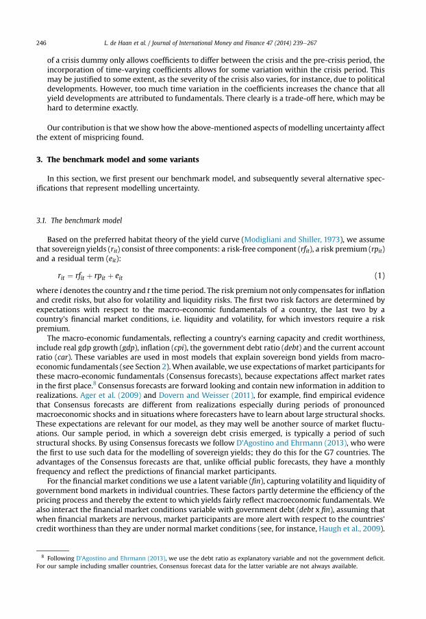
Table 3 does not report estimates for the fixed effects a0i in Model (2). As explained in Section 3,fixed effects represent time-invariant country effects which are related to some unobserved structuralcountry-specific characteristic(s). We report the estimates for the fixed effects in Fig. 4, together withtheir 95% confidence bands.16 The 17th country dummy, which due to the alphabetic order turns out tobe for the United States, is omitted for collinearity reasons. The fixed effects have been centred, so thatthey can be interpreted as deviations from the mean.

Japan stands out with a strongly negative fixed effect of several percentage points. Technically, thiscompensates for the fact that Japan's debt ratio is the highest in the sample while Japan's sovereignyield is relatively low. Economically, this may reflect the relatively large domestic investor base forJapan's sovereign debt, which mostly results from the accumulation of pension savings coupled with astrong home bias (Andritzky, 2012). A similar story e i.e. a relatively high debt ratio and a largedomestically held share of government debt e could explain the also quite sizeable negative fixedeffect for Italy. By contrast, quite sizeable positive fixed effects are found for Ireland and Spain, butmoresurprisingly, also for Sweden and Finland. A possible explanation for Sweden and Finland may be thatthese countries had relative low debt ratios and relatively good growth prospects over the sampleperiod, which may not be fully reflected in the level of long-term yields. A similar story may hold tosome extent for Spain and Ireland. These countries grew fast and had very low debt ratios before thecrisis (Gilbert et al., 2013). Since then, economic fundamentals of these countries deterioratedsignificantly.

6. Results for alternative specifications

In this section we present the results of some alternative modelling choices and sample selections,reflecting the five modelling uncertainties discussed in Sections 2 and 3.

6.1. The calculation of confidence bands for the model prediction (Model uncertainty 1)

We use standard errors which are robust to both autocorrelation and heteroskedasticity. If non-robust (OLS) standard errors would have been used for the calculation of the confidence bands, the

16 The Wald test rejects the null that all fixed effects are jointly equal to zero (F-value ¼ 8.03, p-value ¼ 0.000).


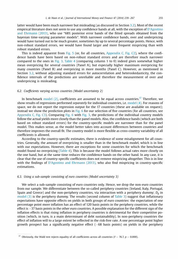
latter would have been much narrower but misleading (as discussed in Section 3.2). Most of the recentempirical literature does not seem to use any confidence bands at all, with the exception of D'Agostinoand Ehrmann (2013), who use “68% posterior error bands of the fitted spreads obtained from thebayesian time-varying parameter models”. With narrower confidence bands, over and underpricingwould have turned out to be much greater, sometimes by up to several percentage points. Hence, withnon-robust standard errors, we would have found larger and more frequent mispricing than withrobust standard errors.

This is indeed apparent from Fig. 5 (or, for all countries, Appendix C, Fig. C2), where the confi-dence bands have been based on non-robust standard errors and are therefore much narrowercompared to the ones in Fig. 3. Table 4 (comparing column 1 to 0) indeed gives somewhat highermean overpricing for several countries (Panel A), but especially higher maximum overpricing formany countries (Panel B) and overpricing in more months (Panel C). However, as mentioned inSection 3.2, without adjusting standard errors for autocorrelation and heteroskedasticity, the con-fidence intervals of the predictions are unreliable and therefore the measurement of over andunderpricing is misleading.

6.2. Coefficients varying across countries (Model uncertainty 2)

In benchmark model (2), coefficients are assumed to be equal across countries.17 Therefore, weshow results of regressions performed separately for individual countries, i.e. model (4). For reasons ofspace, we do not report the regression output for the 17 countries (these are available on request);instead we show the prediction plots in Fig. 6 for our selection of five countries (for all countries, seeAppendix C, Fig. C3). Comparing Fig. 6 with Fig. 3, the predictions of the individual country modelsfollow the actual yieldsmore closely than the panelmodels. Also, the confidence bands (which are bothbased on robust standard errors) for the country-specific models are narrower than for the panelmodel. This makes sense, as the model better takes into account differences between countries andtherefore improves the overall fit. The country model is more flexible as cross-country variability of allcoefficients is allowed.

According to the country-specific estimates, there is evidence of some misalignment for all coun-tries. Generally, the amount of overpricing is smaller than in the benchmark model, which is in linewith our expectations. However, there are exceptions for some countries for which the benchmarkmodel found no overpricing (Table 4). This is because the model follows actual rates more closely onthe one hand, but at the same time reduces the confidence bands on the other hand. In any case, it isclear that the use of country-specific coefficients does not remove mispricing altogether. This is in linewith the findings of D'Agostino and Ehrmann (2013), who also find mispricing in country-specificestimations.

6.3. Using a sub-sample consisting of euro countries (Model uncertainty 3)

We select a sub-sample consisting of euro countries only. Hence, we drop the non-euro countriesfrom our sample. We differentiate between the so-called periphery countries (Ireland, Italy, Portugal,Spain and Greece) and the non-periphery countries, via interaction with a periphery dummy; Dg inmodel (3) is the periphery dummy. The results (second column of Table 3) suggest that inflationaryexpectations have opposite effects on yields in both groups of euro countries: the expectation of onepercentage point more inflation has an effect of 120 basis points in the periphery countries, while theeffect is�37 basis points in the other euro countries. A possible explanation for the different sign of theinflation effects is that rising inflation in periphery countries is detrimental for their competitive po-sition (which, in turn, is a main determinant of debt sustainability). In non-periphery countries theeffect of inflation will to a large extent be reflected in the risk-free rate. A one percentage point highergrowth prospect has a significantly negative effect (�68 basis points) on yields in the periphery

17 Obviously, the Wald test rejects equality of all coefficients across all countries (F ¼ 76.7, p ¼ 0.000).

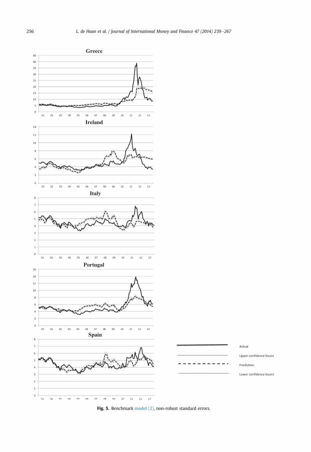
Fig. 5. Benchmark model (2), non-robust standard errors.


Fig. 6. Country-specific estimation, model (4).



countries, but is insignificant in the other countries. The debt ratio has a significant effect of þ0.08 onyields in the periphery, while no significant effect is found for the non-periphery euro countries. Thisconfirms the results of Aizenman et al. (2013b), Poghosyan (2012) and De Grauwe and Ji, (2013a), whofind that yields in the euro area's periphery are higher than in other countries with comparablemacroeconomic fundamentals.

The extent of overpricing is lower according to this model in comparison to both previous models.Only Greece shows substantial mean overpricing (7.3 percentage points) during nine months andIreland shows mean overpricing (1.5) during 15 months (Table 4, column 3, Panels A and C). Twofactors explain this. The first factor is the exclusion of countries outside the euro area with their owncurrency. The second is the fact that we allow markets to react more strongly to fundamentals inperiphery countries. It underlines how sensitive the extent of overpricing is to the selection ofcountries in the sample.

6.4. Financial market conditions (Model uncertainty 4)

To test for the effect of excluding the financial conditions variable on the estimates, we haveestimated model (5). Poghosyan (2012) and De Grauwe and Ji (2013a) do not include such a variable.The results (third column of Table 3) for our sample of 17 countries show that R2 falls to 0.35; hence,the exclusion of financial conditions clearly reduces the overall fit of the model. As a consequence, thepredictions also follow the actual yields less closely than in the benchmark model including fin (Fig. 7for the periphery or Appendix C, Fig. C4 for all countries). However, the exclusion of the financialmarket variable does not completely change the picture for overpricing. The model finds a compa-rable extent of overpricing to our benchmark model for a number of countries, including Greece,Ireland, Spain and Italy (Fig. 7 and Table 4, column 4). Both mean and maximum overpricing aresubstantial in Greece and to a lesser extent Ireland, while Italy and Spain display more limitedoverpricing. However, somewhat surprisingly, the extent of overpricing is reduced compared to ourbenchmark model substantially in Portugal. Again, this is probably because the effect of a generallylower fit on the one hand is compensated by the effect of wider confidence bands on the other. In anycase, an important question remains to what extent financial variables like liquidity should beconsidered as a fundamental.

Many studies use market variables which are uniform to all countries instead of country specific.For example, the VIX index and the TED spread are well-known indicators of market stress (e.g. inHakkio and Keeton, 2009). We also replaced our financial conditions variable by the principlecomponent of the VIX index and the TED spread, as these two series contain highly similar infor-mation. Basically, the results (not reported but available from the authors) confirm the results of themodel excluding the financial conditions variable. This is to be expected, as the VIX-cum-Ted spreadvariable is not country-specific but uniform to all countries and therefore has a similar effect as atime dummy in the panel regression.

6.5. Time variability of the coefficients (Model uncertainty 5)

The benchmarkmodel assumes that all coefficients are constant over time. To relax this assumption,we estimate model (6) interacting all variables with a sovereign crisis dummy variable which has value1 from January 2010 onwards and 0 before. In this way, we can see whether and how the relationshiphas changed because of the European sovereign debt crisis. This approach has also been followed byGiordano et al. (2013) and Beirne and Fratzscher (2013).

From the estimation results (fourth column of Table 3) it can be seen that notably the importance ofgdp has increased significantly during the crisis (at the 5% significance level). The prospect of onepercentage point more growth has an effect of �121 basis points on bond yields during the crisis,compared to �15 before. This result confirms previous findings that markets pay closer attention tomacroeconomic fundamentals during the crisis, which can be seen as a form of wake-up call contagion(Giordano et al., 2013; Beirne and Fratzscher, 2013). Interestingly, our results suggest that during thecrisis markets are particularly worried about the effect of lower economic growth on debt sustain-ability, which confirms results of Cottarelli and Jaramillo (2013).

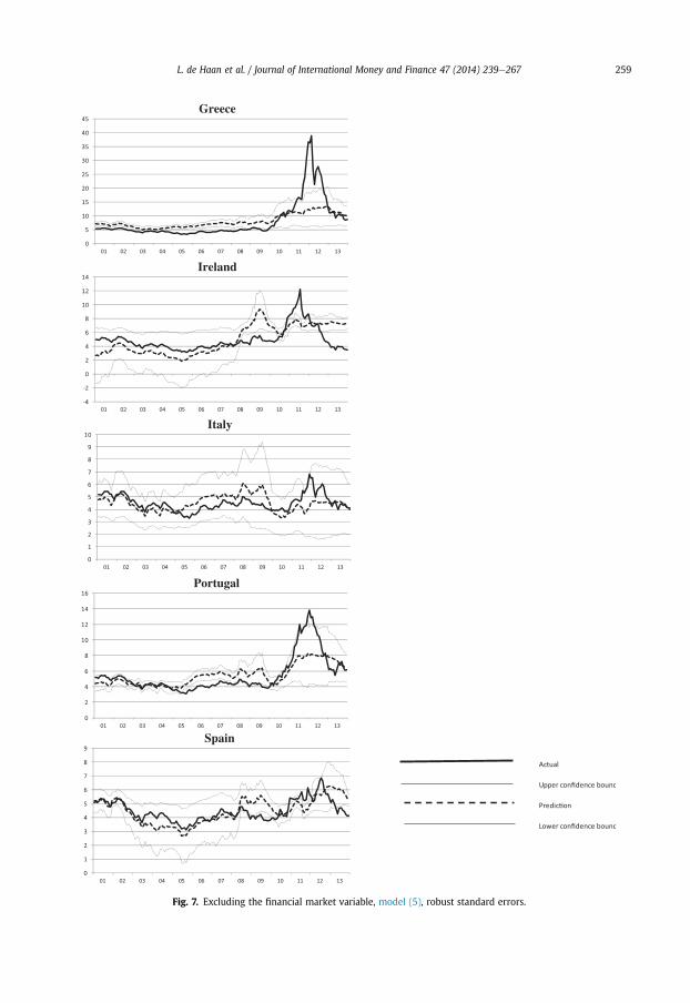
Fig. 7. Excluding the financial market variable, model (5), robust standard errors.



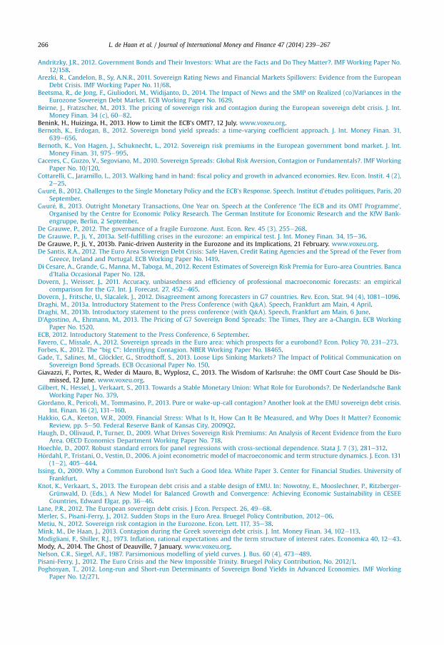
According to this model variant the extent of overpricing is reduced in comparison to the bench-mark model for Portugal. However, overpricing in Ireland is higher. In general, the model shows thatoverpricing is substantial in Greece and Ireland (Table 4, column 5).

6.6. Summary

Table 4 summarizes the extent of misalignment for all six models presented above. It is clear thatthe extent of overpricing depends on the modelling choice. The case of Greece is unambiguous: allmodels suggest mispricing, on average around 700 basis points. Also for Ireland, all models indicateoverpricing, on average within a range of 70e180 basis points. For Portugal, five out of six modelsindicate mispricing, ranging from 20 to 190 basis points. For Belgium, it ranges from 30 to 60 basispoints and for Spain from 30 to 80 basis points. For Italy, mean mispricing ranges from 30 to 50 basispoints.

7. Conclusions

Our results do not point to consistent and massive mispricing of sovereign bond prices ofcountries in the periphery of the Eurozone. A significant part of the increase in yields can beexplained by the deterioration of macroeconomic fundamentals like growth and government debt,while financial variables also played a role in some countries. However, our results do show thatsovereign yields cannot be fully explained by macroeconomic fundamentals alone. This applies inparticular to the countries in the periphery of the euro area. In all model specifications, we findperiods of substantial misalignment of Greek bond yields. Most specifications also indicate someperiods of mispricing for Portugal, Ireland, Spain and Belgium. For Italy, the evidence of mispricing isless strong.

We also find that sovereign yields react more strongly to economic growth prospects during thesovereign crisis (starting January 2010) than before. Within the euro area group of countries, sovereignyields of the countries in the periphery are found to react more strongly to economic growth prospectsas well.

At the same time, modelling uncertainty makes it impossible to determine precisely the extentof misalignment. We show that the extent of overpricing is affected by modelling choices, inparticular with regard to i) the use and calculation of confidence bands for the model prediction, ii)the sample selection, iii) the assumption whether the model coefficients are similar across coun-tries or not, iv) the inclusion of financial variables, and v) the usage of fixed or time-varyingcoefficients.

Unfortunately, it is difficult to determine the relative merit of the various specifications. It cannotbe determined on the basis of econometric diagnostics alone, because a search for possible mispricingdoes not necessarily require the best econometric fit of the model. The choice for a specific specifi-cation therefore also requires economic judgment, and this will by definition always remain subject todebate. Econometric models cannot fully solve the fundamental uncertainty about the fairness ofbond yields.

This has a number of consequences. First, our findings call for modesty in interpreting the outcomesof specific model specifications. Better awareness on how the specific modelling choices affect theextent of mispricing is needed, and a final verdict should preferably be made on the basis of a numberof different specifications. Second, our results call for cautiousness in using estimates of bond yieldmodels in policy making. As models cannot determine mispricing precisely, decisions about possibleinterventions should always be based on a broad set of information criteria, ranging frommodel outputto expert judgment and market evidence. Finally, more research is necessary to determine the causesand nature of mispricing more precisely, in particular with regards to perceptions of political de-velopments and monetary policy decisions.


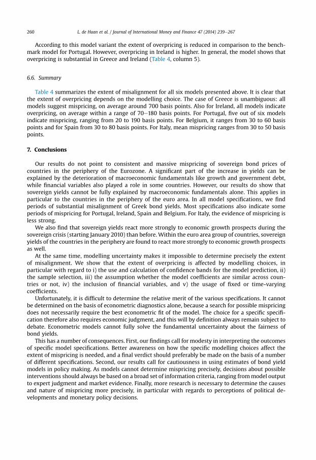
Appendix A. Data definitions and sources

Variable name Description Definition Sources

r Yield on 10 year governmentbonds

Monthly average Datastream

rf Euro overnight index swap rate Monthly average Datastreamcpi Inflation rate, Consensus

forecastMonthly, weighted average fornext 12 months a

Consensus Economics

gdp Real GDP growth rate,Consensus forecast

Monthly, weighted average fornext 12 months a

Consensus Economics

debt Debt ratio, expected Debt ratio minus bal; debt ratioseasonally adjustedand interpolated from quarterlyfigures b

OECD, Consensus Economics

bal Budget balance, % GDP,Consensus forecast


Consensus Economics

fin Financial market conditions.Principal component c

of high-low and bid-ask spreadsd

Monthly average Own calculations basedon Datastream

car Current account ratio,Consensus forecast


Consensus Economics

a If Fym is the Consensus forecast made inmonthm for the current year y, and Fyþ1m is the Consensus forecast for the coming year

yþ1, then the weighted average for the next 12 months is defined as: Fym,ð12�mÞþFyþ1

m ,m12 ; withm ¼ 1; :::;12.

b If bal Consensus forecasts were not available, actual figures have been used.c The principle component is equal to�0.733þ 6.930*high-low spreadþ4.113*bid-ask spread, and is therefore an indicator of

illiquidity and volatililty.d For Greece, bid-ask spreads are not available for most of the sample period. Therefore, fin for Greece has been based on the

high-low spread; for this country, the high-low spread since April 2012 has been kept constant on the level of March 2012 asdata were not available. For several countries, there were only a small number of missing values for high-low and bid-askspreads that have been interpolated.

Appendix B. Levin, Lin and Chu (2002) unit root tests

Ho: Panels contain unit roots

Ha: Panels are stationary

Panel means: Included Included Not included

Time trend: Not included Included Not included

Variable Adjusted t p-Value Adjusted t p-Value Adjusted t p-Value

r �1.395 0.081 �1.723 0.042 �4.500 0.000rf �0.804 0.210 �0.417 0.338 �6.573 0.000cpi �2.020 0.021 �2.640 0.004 �3.959 0.000gdp �2.521 0.005 �0.444 0.328 �6.328 0.000debt 0.302 0.619 �4.016 0.000 2.222 0.986fin �2.695 0.003 �3.946 0.000 �4.496 0.000car 1.669 0.952 4.921 1.000 �1.133 0.128

ADF regressions: 1 lag; Common AR parameter.LR variance: Bartlett kernel, 13 lags average (chosen by LLC).


Appendix C. Figures for all 17 countries

C1. Benchmark model (2), robust standard errors.

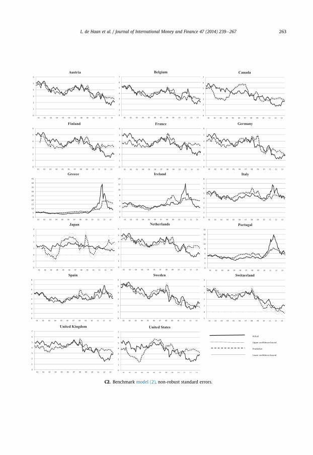
C2. Benchmark model (2), non-robust standard errors.


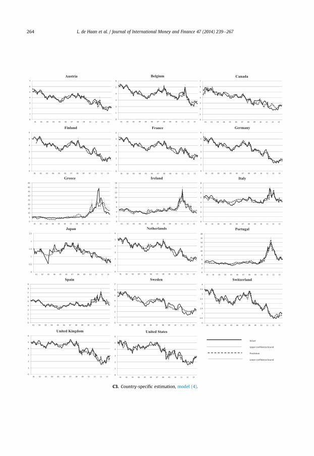
C3. Country-specific estimation, model (4).


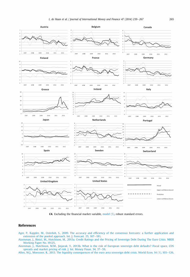
C4. Excluding the financial market variable, model (5), robust standard errors.


References

Ager, P., Kappler, M., Osterloh, S., 2009. The accuracy and efficiency of the consensus forecasts: a further application andextension of the pooled approach. Int. J. Forecast. 25, 167e181.

Aizenman, J., Binici, M., Hutchison, M., 2013a. Credit Ratings and the Pricing of Sovereign Debt During The Euro Crisis. NBERWorking Paper No. 19125.

Aizenman, J., Hutchison, M.M., Jinjarak, Y., 2013b. What is the risk of European sovereign debt defaults? Fiscal space, CDSspreads and market pricing of risk. J. Int. Money Finan. 34, 37e59.

Allen, W.J., Moessner, R., 2013. The liquidity consequences of the euro area sovereign debt crisis. World Econ. 14 (1), 103e126.

http://refhub.elsevier.com/S0261-5606(14)00107-7/sref1











Andritzky, J.R., 2012. Government Bonds and Their Investors: What are the Facts and Do They Matter?. IMF Working Paper No.12/158.

Arezki, R., Candelon, B., Sy, A.N.R., 2011. Sovereign Rating News and Financial Markets Spillovers: Evidence from the EuropeanDebt Crisis. IMF Working Paper No. 11/68.

Beetsma, R., de Jong, F., Giuliodori, M., Widijanto, D., 2014. The Impact of News and the SMP on Realized (co)Variances in theEurozone Sovereign Debt Market. ECB Working Paper No. 1629.

Beirne, J., Fratzscher, M., 2013. The pricing of sovereign risk and contagion during the European sovereign debt crisis. J. Int.Money Finan. 34 (c), 60e82.

Benink, H., Huizinga, H., 2013. How to Limit the ECB's OMT?, 12 July. www.voxeu.org.Bernoth, K., Erdogan, B., 2012. Sovereign bond yield spreads: a time-varying coefficient approach. J. Int. Money Finan. 31,

639e656.Bernoth, K., Von Hagen, J., Schuknecht, L., 2012. Sovereign risk premiums in the European government bond market. J. Int.

Money Finan. 31, 975e995.Caceres, C., Guzzo, V., Segoviano, M., 2010. Sovereign Spreads: Global Risk Aversion, Contagion or Fundamentals?. IMF Working

Paper No. 10/120.Cottarelli, C., Jaramillo, L., 2013. Walking hand in hand: fiscal policy and growth in advanced economies. Rev. Econ. Instit. 4 (2),

2e25.Cœur�e, B., 2012. Challenges to the Single Monetary Policy and the ECB's Response. Speech. Institut d'�etudes politiques, Paris, 20

September.Cœur�e, B., 2013. Outright Monetary Transactions, One Year on. Speech at the Conference ‘The ECB and its OMT Programme’,

Organised by the Centre for Economic Policy Research. The German Institute for Economic Research and the KfW Bank-engruppe, Berlin, 2 September.

De Grauwe, P., 2012. The governance of a fragile Eurozone. Aust. Econ. Rev. 45 (3), 255e268.De Grauwe, P., Ji, Y., 2013a. Self-fulfilling crises in the eurozone: an empirical test. J. Int. Money Finan. 34, 15e36.De Grauwe, P., Ji, Y., 2013b. Panic-driven Austerity in the Eurozone and its Implications, 21 February. www.voxeu.org.De Santis, R.A., 2012. The Euro Area Sovereign Debt Crisis: Safe Haven, Credit Rating Agencies and the Spread of the Fever from

Greece, Ireland and Portugal. ECB Working Paper No. 1419.Di Cesare, A., Grande, G., Manna, M., Taboga, M., 2012. Recent Estimates of Sovereign Risk Premia for Euro-area Countries. Banca

d’Italia Occasional Paper No. 128.Dovern, J., Weisser, J., 2011. Accuracy, unbiasedness and efficiency of professional macroeconomic forecasts: an empirical

comparison for the G7. Int. J. Forecast. 27, 452e465.Dovern, J., Fritsche, U., Slacalek, J., 2012. Disagreement among forecasters in G7 countries. Rev. Econ. Stat. 94 (4), 1081e1096.Draghi, M., 2013a. Introductory Statement to the Press Conference (with Q&A). Speech, Frankfurt am Main, 4 April.Draghi, M., 2013b. Introductory statement to the press conference (with Q&A). Speech, Frankfurt am Main, 6 June.D'Agostino, A., Ehrmann, M., 2013. The Pricing of G7 Sovereign Bond Spreads: The Times, They are a-Changin. ECB Working

Paper No. 1520.ECB, 2012. Introductory Statement to the Press Conference, 6 September.Favero, C., Missale, A., 2012. Sovereign spreads in the Euro area: which prospects for a eurobond? Econ. Policy 70, 231e273.Forbes, K., 2012. The “big C”: Identifying Contagion. NBER Working Paper No. 18465.Gade, T., Salines, M., Gl€ockler, G., Strodthoff, S., 2013. Loose Lips Sinking Markets? The Impact of Political Communication on

Sovereign Bond Spreads. ECB Occasional Paper No. 150.Giavazzi, F., Portes, R., Weder di Mauro, B., Wyplosz, C., 2013. The Wisdom of Karlsruhe: the OMT Court Case Should be Dis-

missed, 12 June. www.voxeu.org.Gilbert, N., Hessel, J., Verkaart, S., 2013. Towards a Stable Monetary Union: What Role for Eurobonds?. De Nederlandsche Bank

Working Paper No. 379.Giordano, R., Pericoli, M., Tommasino, P., 2013. Pure or wake-up-call contagion? Another look at the EMU sovereign debt crisis.

Int. Finan. 16 (2), 131e160.Hakkio, G.A., Keeton, W.R., 2009. Financial Stress: What Is It, How Can It Be Measured, and Why Does It Matter? Economic

Review, pp. 5e50. Federal Reserve Bank of Kansas City, 2009Q2.Haugh, D., Ollivaud, P., Turner, D., 2009. What Drives Sovereign Risk Premiums: An Analysis of Recent Evidence from the Euro

Area. OECD Economics Department Working Paper No. 718.Hoechle, D., 2007. Robust standard errors for panel regressions with cross-sectional dependence. Stata J. 7 (3), 281e312.H€ordahl, P., Tristani, O., Vestin, D., 2006. A joint econometric model of macroeconomic and term structure dynamics. J. Econ. 131

(1e2), 405e444.Issing, O., 2009. Why a Common Eurobond Isn't Such a Good Idea. White Paper 3. Center for Financial Studies. University of

Frankfurt.Knot, K., Verkaart, S., 2013. The European debt crisis and a stable design of EMU. In: Nowotny, E., Mooslechner, P., Ritzberger-

Grünwald, D. (Eds.), A New Model for Balanced Growth and Convergence: Achieving Economic Sustainability in CESEECountries, Edward Elgar, pp. 36e46.

Lane, P.R., 2012. The European sovereign debt crisis. J Econ. Perspect. 26, 49e68.Merler, S., Pisani-Ferry, J., 2012. Sudden Stops in the Euro Area. Bruegel Policy Contribution, 2012e06.Metiu, N., 2012. Sovereign risk contagion in the Eurozone. Econ. Lett. 117, 35e38.Mink, M., De Haan, J., 2013. Contagion during the Greek sovereign debt crisis. J. Int. Money Finan. 34, 102e113.Modigliani, F., Shiller, R.J., 1973. Inflation, rational expectations and the term structure of interest rates. Economica 40, 12e43.Mody, A., 2014. The Ghost of Deauville, 7 January. www.voxeu.org.Nelson, C.R., Siegel, A.F., 1987. Parsimonious modelling of yield curves. J. Bus. 60 (4), 473e489.Pisani-Ferry, J., 2012. The Euro Crisis and the New Impossible Trinity. Bruegel Policy Contribution, No. 2012/1.Poghosyan, T., 2012. Long-run and Short-run Determinants of Sovereign Bond Yields in Advanced Economies. IMF Working

Paper No. 12/271.










http://www.voxeu.org
























































































Steinkamp, S., Westermann, F., 2012. On Creditor Seniority and Sovereign Bond Prices in Europe. University of OsnabrückInstitute of Empirical Economic Research Working Paper No. 92.

von Hagen, J., Schuknecht, L., Wolswijk, G., 2011. Government bond risk premiums in the EU revisited: the impact of thefinancial crisis. Eur. J. Polit. Econ. 27 (1), 36e43.

Weidmann, J., 2012. Money Creation and Responsibility. Speech, Frankfurt am Main, 18 September.Zoli, E., 2013. Italian Sovereign Spreads: Their Determinants and Pass-through to Bank Funding Costs and Lending Conditions.

IMF Working Paper No. 13/84.









Documents

Are European sovereign bonds fairly priced? The role of modelling uncertainty