Are Credit Ratings Still Relevant? ∗

Sudheer Chava

Georgia Tech

Rohan Ganduri

Georgia Tech

Chayawat Ornthanalai

University of Toronto

Abstract

We show that firms’ stock prices react significantly less to credit rating downgrade announce-

ments when they have Credit Default Swap (CDS) contracts trading on their debts. We find

that information in CDS spreads predict firms’ future rating downgrades and defaults, and doc-

ument a significant information flow from the CDS to equity and bond markets before firms are

downgraded. Further, term structures of CDS can be used to construct a more reliable measure

of default risk premium for firms undergoing rating revisions. While the CDS market is not a

perfect substitute for credit ratings, our results suggest that credit rating revisions have become

less informative to equity investors in the presence of the CDS market.

JEL Classification: G12.

Keywords: Credit ratings; Credit default swaps; Financial regulations.

∗Sudheer Chava can be reached at Scheller College of Business at the Georgia Institute of Technology, 800 W.Peachtree St NW, GA 30309-1148; Phone: 404-894-4371; Email: sudheer.chava@scheller.gatech.edu. Rohan Gan-duri can be reached at Scheller College of Business at the Georgia Institute of Technology, 800 W. Peachtree St NW,GA 30309-1148; Phone: 404-894-4371; Email: rohan.ganduri@scheller.gatech.edu. Chayawat Ornthanalai can bereached at Rotman School of Management at the University of Toronto, 105 St.George St, Toronto, ON, Canada, M5S3E6; Phone: 416-946-0669; Email: chay.ornthanalai@rotman.utoronto.ca. We are grateful to the Q-group for finan-cial support and the program committee of 2013 Western Finance Association Annual Meeting for selecting the paperfor the program. We would like to thank Jan Ericsson, Kris Jacobs, Robert Jarrow, Narayan Jayaraman, Lars Norden,Stuart Turnbull, seminar participants at Scheller College of Business, Georgia Tech, Southern Methodist University,University of Alberta, Bank of Canada, University of Oklahoma, University of Maastricht, University of Rotterdam,European School of Management and Technology, Berlin, 2012 European Finance Association Annual Meeting, FirstIFSID Conference on Structured Products and Derivatives, and the 23rd Derivatives Conference at FDIC for helpfulcomments and suggestions. We are responsible for all errors.

1 Introduction

Credit rating agencies that specialize in assessing the credit worthiness of bond issuers are an integral

component of the financial landscape. Investors, regulators, and managers have historically relied on

credit ratings, yet they are also frequently criticized for their slow response in predicting corporate

defaults (e.g., Enron, Worldcom), accuracy of their ratings, and the conflicts of interest inherent in

the agencies’ business model (see White (2010)). As a consequence of these criticisms, regulators

have initiated proposals in the Dodd-Frank Act to reduce regulatory and supervisory reliance on

credit rating agencies.

A firm’s credit rating is the opinion of a particular credit rating agency about the firm’s credit

worthiness, and it reflects the agency’s view on the firm’s physical default probability PDP. The pre-

vailing consensus is that such opinion by a rating agency is relevant as documented by negative stock

market reactions to rating downgrade announcements (see for example Hand, Holthausen, and Left-

wich (1992); Dichev and Piotroski (2001); Jorion, Liu, and Shi (2005)). In contrast, CDS contracts

are a market-based measure of a firm’s default risk, and provide an estimate of the firm’s risk-neutral

default probability PDQ (see Longstaff, Mithal, and Neis (2005)). Although credit ratings and CDS

spreads provide an assessment of the firm’s default risk under two different probability measures

(P versus Q), insights from the structural model suggest they share common information about the

firm’s fundamentals. If CDS spreads provide information about the underlying firm, in lieu of, or in

addition to that conveyed by credit ratings, rating change announcements should become less pricing

relevant to equity investors. In this paper, we analyze whether the stock market still reacts to credit

rating agencies’ downgrade announcements after CDS trades on their underlying firm’s debt.

We use a comprehensive sample of credit rating change announcements from the three major

credit rating agencies — Standard and Poor’s, Moody’s, and Fitch, and we find that, consistent with

the prior literature, stock and bond markets react significantly negatively to credit rating downgrades.

However, when CDS contracts are introduced on the firm’s debt, the stock market reaction to credit

rating downgrades is muted compared with the period before CDS contracts start trading on a firm’s

debt. Also, stock and bond prices of firms with traded CDS contracts react significantly less to rating

downgrades relative to those of firms without traded CDS contracts. These results are robust to a

number of tests such as instrumental variable regressions and propensity score matching analysis,

which were used to mitigate endogeneity concerns.

1

In order to understand the information content of CDS contracts relative to credit ratings, we first

construct CDS-implied credit ratings non-parametrically following the approach in Breger, Goldberg,

and Cheyette (2003) and Kou and Varotto (2008) and find that they start deteriorating 180 days

prior to a downgrade. Second, using a semi-parametric hazard model (See Shumway (2001) and

Chava and Jarrow (2004)), we find that CDS spreads contain information that significantly predict

the likelihood of rating downgrade announcements. In the same vein, we show that information in

CDS spreads complements credit ratings by enhancing corporate default prediction models.

Bond yields also reflect the market’s assessment of a firm’s default risk. However, CDSs are

standardized credit derivative contracts that generally trade more liquidly than bonds and allow

investors to more easily short or hedge credit risk. Further, Longstaff, Mithal, and Neis (2005) and

Ericsson, Jacobs, and Oviedo (2009) show that CDS spreads are a “more pure” measure of a firm’s

default risk than corporate bond spreads (also see Veronesi and Zingales (2010) and Stulz (2010)).

Using the Hasbrouck’s (1995) information share measure, we show the CDS market, on average,

dominates the bond market in credit price discovery (see also, Blanco, Brennan, and Marsh (2005)).

However, before rating downgrades, the CDS market’s information share increases substantially to

about 90% relative to the bond market. Thus, the CDS market is a leading venue for credit price

discovery before rating downgrade announcements.

The presence of the CDS market can also helps improve equity valuation. Examining the infor-

mation flow between the CDS and stock markets, we find that unanticipated changes in CDS spreads

lead stock returns, predominantly before firms are downgraded. In support of our main conclusion,

we find evidence suggesting that stock prices react less to rating change announcements because a

bulk of their price adjustment occurred in the pre-announcement period.

An important channel through which the CDS market improves equity pricing is by providing

investors with information that can be used to better estimate the default risk premium. In particular,

Avramov, Chordia, Jostova, and Philipov (2009) find that the distress risk puzzle, i.e., lower rated

firms earn lower returns, is most pronounced around rating downgrades.1 We test this implication

by examining the value of the CDS market in explaining the cross-section of stock returns for firms

that are about to be re-rated. We follow the method developed in Friewald, Wagner, and Zechner

(2014). Their general idea is that the firm’s equity risk premium can be extracted using the term

1For the review of literature, see Campbell, Hilscher, and Szilagyi (2008) and Chava and Purnanandam (2010).

2

structure of CDS spreads over time. Our results, based on portfolio sorting, show a strong, positively

monotonic relationship between CDS-implied equity risk premia and average one-year equity returns.

Importantly, this finding holds when we focus our samples on firms that are about to be downgraded.

However, we observe the opposite pattern — i.e., firms with higher default risk have lower returns,

when sorting firms based on credit rating levels.

Our paper contributes to two strands of literature. The first is the literature documenting ab-

normal stock and bond market returns to credit rating downgrades, but not for upgrades.2 Jorion,

Liu, and Shi (2005) argue that the Regulation Fair Disclosure (Reg FD) might have bestowed upon

the credit rating agencies an informational advantage owing to the exemption of the rating agencies

the regulation.3 Our results show that even after Reg FD, the onset of CDS trading significantly

reduces the importance of these rating change announcements.

The second strand of literature two which we contribute is related to studies that examine whether

the CDS market helps in price discovery. For example, Hull, Predescu, and White (2004), and Norden

(2011) show that CDS spreads anticipate credit rating downgrades, and some evidence exists that

CDS spreads lead the stock (Acharya and Johnson (2007)) and bond market (Blanco, Brennan, and

Marsh (2005)) in price discovery. Motivated by these studies, we examine whether stock and bond

markets perceive credit rating announcements to be less pricing relevant when the underlying firm

has a CDS contract traded on its debt.

Any market based benchmark of default risk, such as CDS, provides a risk-neutral assessment of

default risk. However, credit ratings which convey the agency’s objective view of a firm’s default risk

are built “through the cycle” and may be more suitable from a corporate policy or a risk-management

perspective. So, without making additional assumptions, CDS contracts and credit ratings are not

completely equivalent and hence not a perfect substitute. Similar to credit ratings, CDS can convey

many false positives. Furthermore, as with any market-based measures, changes in CDS spreads can

be volatile, which may make them less suitable for use as a benchmark in financial contracts such has

bond covenants or rating triggers. Credit rating agencies can still play an important role in financial

markets, but the increased competition from the CDS markets and the availability of a market-based

benchmark for default risk can potentially improve the performance of rating agencies.

2For examples, see Holthausen and Leftwich (1986), Hand, Holthausen, and Leftwich (1992), Goh and Ederington(1993), and Dichev and Piotroski (2001).

3We confirm the finding in Jorion, Liu, and Shi (2005) on the effect of Reg FD introduced in August 2000.

3

The rest of this paper is organized as follows. Section 2 develops hypotheses that motivate

empirical tests in this paper. Section 3 describes the data. Section 4 presents the main empirical

tests of stock price reactions to rating revisions. Sections 5 and 6 examine why stock prices react

significantly less to credit rating downgrades in the presence of CDS contracts. Section 7 examines

the value of CDS contracts for explaining the cross-section of stock returns in relation to default risk

premia. Finally, Section 8 concludes.

2 Hypotheses development

In this section, we develop hypotheses that motivate subsequent empirical tests using insights based

on static analysis of the Merton (1974) structural model. Merton (1974) assumes the firm value V

follows a geometric Brownian motion with drift µ and volatility σ. The model values equity E as a

call option on the firm value with the strike price equal to the face value D of a non-coupon paying

bond with maturity T. The firm can default only at the maturity T of its debt. It can be shown

that the expected excess equity return over the risk-free rate µE − r (i.e. equity risk premium), and

the equity volatility σE are given by

µE − r = (µ− r)(V

EEV

)(1)

σE = σ

(V

EEV

), (2)

where EV denotes the partial derivative of E with respect to V . Using standard call option pricing

notation for E, and noting that EV is the call option delta, we can rewrite equation (1) as

µE − r =µ− r

1− Le−rT[

Φ(d2)Φ(d1)

] , (3)

where L =D

Vis the firm’s leverage, and Φ denotes the cumulative distribution function of the

standard normal random variable.4 Equation (3) shows that the firm’s equity risk premium is a

function of its asset return, asset return volatility, and leverage. For instance, ceteris paribus, a

shock to the firm’s asset return µ is amplified when translated to a change in the firm’s equity return

4In the standard Black-Scholes option pricing formula, d1 =log(V/D)+(r+ 1

2σ2)T

σ√T

, and d2 = d1 − σ√T

4

due to the leverage effect.

The default probabilities under the physical measure (PDP) and the risk-neutral measure (PDQ)

are respectively given by

PDP = Φ

(−log(1/L) + (µ− 1

2σ2)T

σ√T

)(4)

PDQ = Φ

(−log(1/L) + (r − 1

2σ2)T

σ√T

). (5)

Combining equations (4) and (5) and using the relationships shown in equations (1) and (2), we can

write the equity risk premium as

µE − r =(

Φ−1(PDQt )− Φ−1(PDP

t )) σE√

T. (6)

Equation (6) shows that changes to PDP and PDQ can affect the equity risk premium thereby

resulting in the stock price reaction. Therefore, we expect the stock price to react to new information

about the firm’s physical and risk-neutral default probabilities.

A credit rating, by definition, conveys the rating agency’s opinion about the firm’s ability to meet

its financial obligations on time.5 Therefore, a rating change reflects the change of an agency’s view

on the firm’s physical default probability PDP. A related question is what new information about

the firm’s fundamentals does it contain? Equations (3) and (4) provide some insights. For instance, a

rating downgrade, which corresponds to an increasing PDP can be due to a deterioration in the firm’s

performance (decreasing µ, ∂PDP

∂µ < 0) or uncertainty of its cash flows (increasing σ, ∂PDP

∂σ > 0), or

both. As a result, stock prices react negatively to unanticipated bad news about µ and σ because

∂ERP∂µ > 0, and ∂ERP

∂σ < 0. An increase in PDP can also arise due to the change in firm leverage L as

seen from ∂PDP

∂L > 0, but this leads to a positive stock market reaction as ∂ERP∂L > 0. Distinguishing

between which information change conveyed by rating agencies is more relevant to equity investors

can be difficult.6 Because we do not observe the exact reason in terms of the change in fundamentals

that drives the rating change event, we include all the rating change announcements in our analysis.

5For instance, Standard & Poor’s website states that credit ratings express the agency’s opinion about the abilityand willingness of an issuer, such as a corporation or state or city government, to meet its financial obligations in fulland on time.

6Goh and Ederington (1993) documented that rating changes – specifically downgrades – due to a deterioration infirm’s financial prospects are informative and produce a negative abnormal stock return while those due to an increasein leverage are uninformative.

5

Our first hypothesis relates to the information relevance of credit rating agencies. If credit

ratings provide equity investor with pricing-relevant information about that firm’s physical default

probability, then rating change events should elicit stock market reactions.

Hypothesis 1 The stock market reacts to a firm’s credit rating change announcement as the news

reveals changes in the firms physical default probability.

The simple structural model offers us insights into how the presence of the CDS market may affect

the value of credit rating changes. CDS spreads embody a risk-neutral assessment of the firm’s

default probability PDQ. Taking partial derivatives of PDP and PDQ (see equations (4) and (5))

with respect to σ, L, and µ, respectively, shows that (1) ∂PDQ

∂σ > 0, ∂PDP

∂σ > 0; (2) ∂PDQ

∂L > 0 , ∂PDP

∂L >

0; and (3) ∂PDQ

∂µ = 0 , ∂PDP

∂µ > 0. These relationships suggest that the risk-neutral default probability

PDQ and the physical default probability PDP contain correlated information about the firm’s

fundamentals (i.e., regarding σ and L). Therefore, if the CDS market provides information about

the underlying firm’s fundamentals, in lieu of, or in addition to that conveyed by credit ratings

(through PDP), then rating change announcements should become less pricing relevant to equity

investors.

Hypothesis 2 Stock market reactions to a firm’s rating change events are attenuated if CDS con-

tracts trade on the underlying firm’s debt.

The hypothesis above tests for the effect of CDS trading on the value of rating changes, which is

the main conclusion of this paper. In the remaining hypotheses, we focus on how and why the CDS

market may affect the magnitude of stock market reactions to credit rating changes.

As discussed previously, static analyses of the structural model show that CDS spreads and

credit ratings convey common information about the firm’s fundamentals. If CDS spreads contain

information about the firm that anticipates changes in PDP associated with rating revisions, then

rating change announcements should become less informative about the firm’s equity risk premium.

This, in turn, implies a smaller stock market reaction to rating change announcements.

Hypothesis 3 CDS spreads contain information that predict credit rating revisions.

We test the hypothesis above by examining whether CDS spreads predict rating changes on a firm,

and whether they improve the model for predicting defaults.

6

The presence of CDS market can improve equity valuation, if it contains new information about

the firm’s risk-neutral default probabilities (see equation (6)). Although CDS and corporate bond

spreads provide a risk-neutral assessment of their underlying firm’s default risk, existing evidence

suggests that the CDS market leads the bond market in credit price discovery (see Blanco, Brennan,

and Marsh (2005)). CDS contracts also provide a feasible way to short credit risk, thereby helping

complete the credit risk market.7 Until then, shorting corporate bonds was limited to the repo

market which typically has very short maturity. Whereas CDS contracts are standardized and can

be used for shorting credit risk for longer periods ranging from one to ten years. Further, the CDS

market generally trades more frequently relative to the corporate bond market. This enables market

participants to construct high frequency estimates of risk-neutral default probability.

Equity prices also contain information about the firm’s credit risk. However, Acharya and John-

son (2007) find that changes in CDS spreads lead stock returns especially around negative credit

events. They argue that unlike the stock market, trading in the CDS market is dominated by large

institutions, mostly banks, which explains why the information revelation may occur in the CDS

market before the equity market. In relation to credit rating changes, if the CDS market provides

new information about the firm’s credit risk before rating change announcements, we expect unantic-

ipated changes in CDS spreads to lead stock and bond returns during this period. As a result, stock

prices react less to rating change announcements because a bulk of their price adjustment occurred

in the pre–announcement period.

Hypothesis 4 CDS spreads lead other market measures that embody risk-neutral default probabilities

before rating change announcements.

We test the hypothesis above by examining whether the CDS market contributes to price discovery

in the stock and bond markets before rating change announcements.

Arguments in Hypotheses 2–4 posit that the presence of CDS market improves equity valuation

by providing investors with new (or more reliable) information about the firm’s credit risk. This

statement has an important implication in light of the well documented distress risk puzzle, i.e., lower

rated firms earn lower returns, because the structural model shows that risk premia in equity and

credit markets are related (see equation (6)). In particular, Avramov, Chordia, Jostova, and Philipov

(2009) find that the puzzle is most pronounced around rating downgrades. Therefore, if the CDS

7See Flannery, Houston, and Partnoy (2010) for supporting arguments.

7

market provides information that improves equity valuation, we expect equity risk premia estimated

using CDS information to relate better to firms’ default risks than credit ratings, particularly for

firms that are about to be re-rated. We test this important implication in the next hypothesis.

Hypothesis 5 The CDS market provides investors with a more reliable measure of default risk

premium than credit ratings for firms undergoing rating revisions.

To test the hypothesis above, we examine whether the equity risk premia extracted from CDS data

can explain the cross-section of stock returns of firms that are undergoing rating revisions.

3 Data and descriptive statistics

We use a CDS database that is widely used among financial market participants (CMA Datavision

database (CMA)) to identify all firms for which we observe CDS quotes on their debt. CMA contains

consensus data sourced from 30 buy-side firms, including major global investment banks, hedge funds,

and asset managers which is disseminated through Bloomberg since October 2006.8 We further

ensure the accuracy in the coverage of CDS quotes by augmenting the CMA database with CDS

data obtained from Bloomberg. The earliest quotes were then taken as the first sign of active CDS

trading on a firm’s debt.

Data on bond ratings were gathered from the Mergent Fixed Income Securities Database (FISD).

FISD provides comprehensive data on issue-level details on over 140,000 corporations, U.S. agencies,

and U.S. Treasury debt securities. The data contains detailed information for each issue, including

the issuer name, rating date, rating level, agency that rated the issue, and credit watch status, etc.

We include only those ratings issued by the top three NRSROs – S&P, Moody’s, and Fitch. We

restrict our sample to U.S. domestic corporate debentures, and exclude yankee bonds, and bonds

issued via private placements, preferred stocks, mortgage-backed, trust preferred capital, convertible

bonds and bonds with credit enhancements. We also consider only the issuers whose stocks are

traded on either the NYSE, AMEX, or NASDAQ. Approximately 18% of the ratings are from Fitch,

and the remaining ratings are split evenly between S&P and Moody’s.

We consider a rating change for an issuer as one observation. When there are rating changes on

8Mayordomo, Pena, and Schwartz (2010) compare the data qualities of the six most widely used databases – GFI,Fenics, Reuters, EOD, CMA, Markit and JP Morgan – and find that the CMA database quotes lead the price discoveryprocess.

8

multiple bond issues for an issuer on the same day, we use the issue with the greatest absolute rating

scale change because such changes are likely to create the strongest impact on bond and stock prices.

We consider only the rating announcements that are associated with either “DNG” (downgrade) or

“UPG” (upgrade), which constitute about 90% of the total rating events.9 The main sample is from

January 1996 to December 2010 and consists of 4665 downgrades and 2171 upgrades; we refer to

it as the “Full sample” for the remainder of this paper. The Full sample consists of 1142 unique

firms, of which 390 have CDS trading at some point during the sample period. There are about 2.1

downgrades for every upgrade, which is line with the findings in Dichev and Piotroski (2001). More

details on the sample are provided in the internet appendix.

Many of the firms in our sample never experienced CDS trading over the 1996-2010 period. In

order to control for the differences between firms with and without CDS contracts traded on their

debt, we consider a subsample of firms for which CDS starts trading at some point during our sample

period. We refer to this sample as the “Traded-CDS”. We use firms’ rating changes in this subsample

to compare their stock reactions to rating change announcements made between their pre-CDS and

post-CDS trading periods. The average size of rating change for the sample is 1.45 before CDS

trading starts and 1.49 after CDS trading starts. The distribution of the rating changes are provided

in the internet appendix.

We obtain corporate bond price data from TRACE, which contains individual bond transactions

starting on July 1, 2002. Corporate bond data prior to July 2002 is obtained from Mergent FISD

historical NAICS database. We apply a number of standard filters to the data set. Following

Bessembinder, Kahle, Maxwell, and Xu (2009), we eliminate trades that have been canceled or

corrected, trades that have commissions, and non-institutional trades because they show that they

help increase the power of the test for detecting abnormal performance. Therefore, consistent with

Edwards, Lawrence, and Piwowar (2007), we remove observations in which the par value of the

transaction is less than or equal to $100, 000 because smaller trades tend to be non-institutional

trades.10

9The FISD ratings database reports the reason for the rating change on an issue. About 4.8% of the total ratingchange reasons are “IR” (Internal Review), while about 2% are “AFRM” (Affirmed).

10The prices reported in the TRACE bond database are the “clean” prices. They do not include the accrued couponpayment. We add the accrued coupon payment to the clean prices by merging in variables from the Mergent FISDdatabase. The final bond prices that we use are therefore settlement prices.

9

4 Stock price reaction to rating changes

This section tests Hypotheses 1 and 2 of the paper. First we provide univariate evidence that the stock

market reacts to rating downgrades, but the magnitude significantly decreases when CDS contracts

trade on the firm’s debt. We then confirm our results using multivariate regressions. Subsequently,

we address endogeneity concerns regarding to the timing of the CDS introduction.

4.1 Abnormal stock returns

We study changes in daily abnormal stock returns on the date of rating change announcements for

CDS and non-CDS firms. We carry out the analysis separately for upgrades and downgrades. We

define the daily abnormal stock return of firm i on day t, ARit, as the residual estimated from the

market model:

ARit = Rit − (αi + βiRmt),

whereRit is the raw return for firm i on day t, andRmt is the value-weighted NYSE/AMEX/NASDAQ

index return. We examine whether the mean cumulative abnormal return (CAR) around the event

period is significantly different from zero. Following Holthausen and Leftwich (1986), we compute

CAR using the three-day window centered on the announcement date. That is, CARi(−1, 1) =∑+1t=−1ARit. Kothari and Warner (2007) show that short–horizon event studies such as ours are not

highly sensitive to the assumption of cross-sectional or time-series dependence of abnormal returns,

as well as the benchmark model used for computing abnormal returns.11

4.2 Univariate analysis

Table 1 presents the mean of cumulative adjusted return (CAR) for the pre- and post-CDS trading

periods. The results in Panel A are based on the “Full-sample” which, consists of traded-CDS and

non-traded-CDS firms. The results in Panel B are based on the “Traded-CDS–sample”. Traded-CDS

firms are those that have CDS traded at some point during our sample period. However, non-traded-

CDS firms are those that do not have CDS trading in our sample period, which is from 1996 to 2010.

Results obtained using the “Traded-CDS–sample” can be usefully thought of as fixed-effects tests

11We estimate αi and βi using a rolling window over a period of 255 days from -91 to -345 relative to the eventdate. Using a shorter estimation window and a different factor model do not affect our conclusions. Table I.A1 inthe Internet Appendix shows that we obtain similar findings when using the Fama-French 3-factor model to calculateabnormal return.

10

because only firms that experience CDS trading are considered. Consistent with previous studies,

Panel A shows that overall, stock price reacts significantly to downgrades (-4.31%) but only weakly

to upgrades (0.14%).12 This finding supports of Hypothesis H1.

The results in Panel A show the mean CARs over the three-day window around rating downgrades

is negative and significant at the 1% level for the pre- and post-CDS periods. However, the magnitude

is significantly weaker for the post-CDS period. The mean CAR in the post-CDS period is -2.51%,

compared to -5.10% in the pre-CDS period. The difference in CAR between these two groups is

2.58% and is statistically significant at the 1% level. On the other hand, we do not find that stock

prices react significantly differently to rating upgrades in the post-CDS period. The difference in

CAR to credit rating upgrades do not differ significantly between the pre- and post-CDS periods.

In Panel B of Table 1, we report univariate results for firms that eventually have CDS contracts

traded on its debt. Restricting our analysis to the Traded-CDS sample mitigates the concern that

traded-CDS firms are inherently different from non-traded-CDS firms. We find that stock price

reaction to credit rating downgrades is significantly weaker in the post-CDS period. The difference

in the mean CAR values is -0.95% between the pre-CDS and post-CDS periods, and is statistically

significant.13

4.3 Regression analysis

We employ multivariate regressions to control for factors that could affect stock price reactions

to rating changes. Following previous studies (e.g., Holthausen and Leftwich (1986)), we run the

regressions separately for upgrades and downgrades. The results are reported in Table 2. The

regression model that we estimate is

CARi =β0 + β1dCDSi +∑

γiRating-level characteristicit+∑δiFirm-level characteristicit +

∑φiCDS-trading control it + εi

(7)

where for bond issue i, CAR is the 3-day cumulative abnormal return centered on the date of rating

change announcements – i.e., event window (-1,1). The main variable of interest is dCDS, an

12The magnitude of CAR to rating downgrades is in line with existing studies that examine announcement returnsto rating changes using the more recent sample, e.g. Jorion, Liu, and Shi (2005).

13Jorion, Liu, and Shi (2005) find that stock price reactions to rating downgrades is significantly stronger afterRegulation Fair Disclosure (Reg FD) was implemented in Oct 2000 because rating agencies are exempt from Reg FDand could still access private information on the rated firms. For a robustness check, we eliminate rating changes priorto the year 2001 (before Reg FD was put in place) and find that our conclusions remain unchanged.

11

indicator variable equal to one if the rating change takes place when CDS trades on the underlying

firm and 0 otherwise. Panel A of Table 2 reports results for rating downgrades, while Panel B reports

results for rating upgrades. Each panel reports results for three regression specifications. Regression

models (I) and (II) are run on the full sample, while regression model (III) is estimated using the

traded-CDS sample. All variables are defined in Appendix B.14

If rating changes are less informative in the presence of CDS trading, we would expect the

coefficient of dCDS in equation (7) to be positive for downgrades and negative for upgrades. Panel

A of Table 2 shows the coefficients on dCDS are positive and statistically significant across the three

regression specifications. Controlling for industry- and year-fixed effects in specification (II), we find

the difference in CARs between firms that have and do not have CDS trading is 1.70%. Looking only

at the traded-CDS sample, (i.e. model (III)), we find the evidence is stronger. Stock prices react

significantly less to credit rating downgrades by an average of 2.59% in the traded-CDS sample. The

results in Panel B, however, show that all three coefficients on dCDS are not significantly different

from zero. Overall, our regression results in Table 2 confirm our univariate results (see Table 1) that

stock price reaction is significantly weaker to credit rating downgrades, and not upgrades, when CDS

contracts trade on the firms’ debt.

The coefficients on the control variables are in line with the results documented in the literature

(see Hand, Holthausen, and Leftwich (1992), and Jorion, Liu, and Shi (2005)). Table 2 shows the

coefficients on Previous Rating and AbsRating Change are negative and highly significant, suggesting

that ratings downgrades on lower-rated firms, as well as downgrades across multiple cardinal scales,

lead to larger stock price reactions. The time since the previous credit rating does not seem to

impact how the new rating change influences stock response. However, rating downgrades accom-

panied by firms’ earnings announcements elicit a larger stock price reaction. Among the firm-level

characteristics, we find that firms’ recent return performances, (i.e. Avg Return), robustly predict

the magnitude of stock price reactions to rating downgrades. Leverage, as well as Avg Trading Vol-

ume appear to be negatively related to CAR for downgrades, though, their statistical significance

14All regression models include three sets of control variables to account for potential factors affecting the magnitudeof stock price reactions. The first set of control variables are rating-level characteristics: previous rating level, thesize of rating change, how long has the previous rating been outstanding for, and whether rating change occurs inrelation with the company’s earnings announcement. The second set of control variables includes various firm-levelcharacteristics. The third set of control variables account for characteristics that may be related to the propensity thatfirms that have CDS trading. All variables are defined in Appendix B. All firm-level characteristics and CDS-tradingcontrols are lagged by one period, i.e. a month or a quarter, depending on the frequency of data sources.

12

disappears when we restrict our regressions to traded-CDS firms.

We confirm that our regression results are robust to a series of robustness checks, which are

reported in the Internet Appendix. Table IA3 Panel A reports regression results showing that our

main conclusion holds when we allow for Industry×Year fixed effects, which helps controlling for

time-varying industry risk factors. Table IA3 Panel B shows our regression results hold when using

a subsample of only non-financial firms. We find that the coefficients on dCDS are slightly larger in

magnitude for downgrades when we focus our analysis only non-financial firms. Further, to ensure

that our results are unaffected by the financial crisis, we focus on rating changes prior to 2008 and

find that our conclusions remain intact. Table IA4 Panel A replicates the results in Table 2 using the

Fama-French 3-factor model to compute CARs and Table IA4 Panel B conducts a pooled analysis

on downgrades and upgrades together. In both cases we verify that our results are robust.

4.4 Instrumental variable analysis

A potential concern with any study on the impact of the CDS market is that the timing of CDS

introduction is not exogenous. CDS contracts may have been introduced during a period when the

firm’s credit quality improves, thereby affecting how its stock price reacts to rating changes. In this

section, we address the concern that the emergence of the CDS market is not exogenous using the

instrumental variable method.

We follow Saretto and Tookes (2013) to find an instrument that correlates with the firm’s like-

lihood of having CDS contracts traded on its debt, while being directly unrelated to how the firm

reacts to its credit rating changes. Saretto and Tookes (2013) use the foreign exchange derivatives

traded for hedging purposes by banks that have a lending relationship with a given firm as the in-

strument for CDS market introduction. The choice of this instrument is motivated by Minton, Stulz,

and Williamson (2009) who show that banks that use interest rate, foreign exchange, equity, and

commodity derivatives are more likely to be net buyers of CDS, and hence related to the emergence

of the CDS market. Among banks’ various derivatives activities, their foreign exchange position is

arguably least likely to directly influence the credit risk of firms with which they conduct business.

Importantly, the amount of foreign exchange derivatives used by banks reflect their hedging need for

macro risk, and hence should not affect the credit risk of domestic firms (i.e., U.S. entities) in our

sample. We further exclude non-financial firms from the instrumental variable regression results for

13

two reasons. First, financial firms are more likely to act as borrowers and lenders amongst them-

selves and with several banks simultaneously, which makes their nature and the extent of relationship

difficult to identify. Second, we want to maintain consistency with Saretto and Tookes (2013) who

motivated the use of the instrumental variable.

Our instrumental variable, Forex Derivative Hedging, is defined as the average foreign exchange

derivatives amount used for hedging (i.e., non-trading purposes) relative to total assets by the lead

syndicate banks and bond underwriters that the firm has conducted business with over the past five

years. We use the Dealscan syndicated loan database to identify firms’ lenders (i.e., lead syndicates),

and Mergent FISD database to identify firms’ bond underwriters. Banks’ derivatives usage data is

obtained from the Bank Holding Company (BHC) Y9-C filings. We lag Forex Derivative Hedging

by one quarter when including it in the instrumental variable (IV) estimation. The average Forex

Derivative Hedging at the firm-level in our full sample is 1.98% of the total assets with a standard

deviation of 1.54%. These values are in line with Saretto and Tookes (2013).

In order to address concerns that CDS introduction is endogenous, we re-estimate the main

regression results using Foreign Derivative Hedging to instrument for dCDS. We follow Wooldridge

(2001) and apply the fitted variable from a probit model for dCDS to the regression model in equation

(7); see also Bharath, Dahiya, Saunders, and Srinivasan (2007) and Saretto and Tookes (2013) for

similar applications. We include firm-level characteristics and CDS-trading controls in the probit

model. The instrument that we use is available quarterly and therefore the model is estimated at

the firm-quarter level. Table B2 in the Appendix reports the probit model from the IV estimation.

After accounting for various firm-level characteristics and variables that may influence CDS trading,

we find that the amount of foreign derivatives usage significantly predicts the likelihood that a firm

will have CDS trading on its debt (t-statistic of 4.84).15

Table 3 reports the regression results using the fitted instrumental variable, dCDS IV for 1966

downgrades and 886 upgrades belonging to 609 unique firms. The number of observations are lower

compared to Table 2 because we restrict our sample to non-financial firms with lending or under-

writing relationships with banks that are active in the forex derivatives market. Further, bank forex

derivatives activities are reported in the BHC Y-9C filings and call reports are from 2001 onwards.

15The incremental psuedo-R2 of the instrument is about 1.1%. The economic impact of foreign exchange derivativesusage on the probability of CDS trading is reasonably large. We find that a one-standard deviation increase in ForexDerivative Hedging increases the likelihood that a firm has CDS traded on its debt by 4.2. Overall, consistent withSaretto and Tookes (2013), we find that the instrument is not weak.

14

Table 3 shows the coefficients on dCDS IV are positive and statistically significant for down-

grades, but not for upgrades, which is largely consistent with our previous findings. A one-standard

deviation change in the dCDS IV is related to a 2.26 and 2.01 percent attenuation in CAR response

to credit rating downgrades for the regressions specifications with industry-fixed effects (I) and year-

and industry-fixed effects (II), respectively. The estimated coefficients on the other variables in Table

3 are similar to those in Table 2 . Overall, we conclude that our main results hold when using Foreign

Derivative Hedging as an instrument to address the potential bias associated with the endogeneity

of CDS market introduction.

4.5 Matched sample analysis

In addition to the instrumental variable regression, we carry out a matched-sample analysis to

mitigate concerns that traded-CDS and non-traded-CDS firms are different on some observable di-

mensions. A traded-CDS firm is matched with a firm that does not have a CDS traded on its debt at

any point in our sample period (i.e., a non-traded-CDS firm). We use a propensity score matching

method that can incorporate a large number of matching dimensions (Rosenbaum and Rubin (1983)).

The matching is carried out in the month when CDS starts trading on a traded-CDS firm based on

15 observable characteristics. These matching characteristics are motivated by Ashcraft and Santos

(2009), Saretto and Tookes (2013), and include other factors that might affect the introduction of

CDS trading.

We estimate firms’ propensity of having CDS trading using a probit model, in which the depen-

dent variable, dCDS, is an indicator variable equal to one starting on the month when CDS begins

trading on the firm, and zero otherwise. All explanatory variables in the probit model are lagged

by one period and defined in Appendix B. We require that firms entering the matching sample have

complete time-series information on their observable variables. This requirement leaves us with 376

traded-CDS firms and 418 non-traded-CDS firms for estimating the propensity score model, which

we refer to as the before-matching sample. In the Appendix, Table B3 reports diagnostics of the

propensity score matched sample. In Panel A, the column labeled “Before matching” reports results

for the probit model estimated at the firm-month level using the before-matching sample. Most of

the estimated coefficients are significant with the magnitude roughly in line with the probit model es-

timated using firm-quarter observations for the instrumental variable estimator (see Table B2). The

15

fitted probability from the probit model is then used as the propensity score to match traded-CDS

firms to non-traded-CDS firms.

For each traded-CDS firm, we use its propensity score in the month that CDS starts trading to

identify a non-traded-CDS firm with the closest propensity score in the same month. We require

that the propensity score of the matched non-traded-CDS firm be within ±5% of the propensity

score of the traded-CDS firm. The matching technique used for this is the nearest-neighborhood

caliper method of Cochran and Rubin (1973). We match one traded-CDS (treated) firm with five

non-traded-CDS firms (control), i.e., one-to-five matching, in order to increase our sample of matched

control firms (see Dehejia and Wahba (2002), and Smith and Todd (2005)). The matching is carried

out with replacement.16 This exercise leaves us with 354 unique traded-CDS firms each matched to

five eligible control firms.

We report various diagnostics of the matched sample in Table B3 in the Appendix. The column

labeled “After matching” in Panel A reports results derived from estimating the probit model using

the matched observations. Overall, the explanatory power of the probit model decreases significantly

with the pseudo R2 of 14% relative to 49% observed in the “Before matching” sample. We find that

four observable characteristics remain statistically significant in the probit model for the matched

sample. Given the large observable dimensions used for matching, i.e., 15 dimensions, we do not

expect to find a perfect match. Nevertheless, Panel A shows that all the probit coefficients in the

after-matching sample either lost statistical significance or have become substantially less significant

relative to the before-matching sample. We further report the quality of our matched sample in

Panels B and C in the Appendix Table B3. In Panel B, we report univariate means of the 15

observable dimensions for the before-matching and after-matching samples. The findings echo the

results reported in Panel A, which show that the propensity-score matching significantly reduces

observable differences between the traded-CDS firms (treatment group) and the non-traded-CDS

firms (control group). Nevertheless, traded-CDS firms in the matched sample still tend to be larger,

better rated, and have greater bond debt outstanding. In order to control for the differences in

these remaining observable dimensions, we include all the matching controls in our matched sample

regressions. Additionally, in Panel C we report the industry distribution of firms in the treatment

16We also verify that our results are similar when using one-to-one matching without replacement. In this case, wehave 242 uniquely matched pairs. Table IA5 in the Internet Appendix reports difference-in-difference regression resultsverifying our main finding using the one-to-one matched sample without replacement.

16

and control samples. Overall, we find that industry distributions of the two samples do not differ

greatly.

Using the matched sample, we estimate the following difference-in-difference regression

CARi = β0 + β1dCDSi + β2dTreatment i + β3 dTreatment i × dCDSi

+∑

γiRating-level characteristicit +∑

δiFirm-level characteristicit

+∑

φiCDS-trading control it + εi,

(8)

where the dependent variable CARi is the cumulative abnormal stock return of firm i to a credit

rating downgrade. Table 4 reports the results. To save space, we do not report results for credit rating

upgrades as our previous evidence suggests that CAR to credit rating upgrades are, on average, not

significant. The above regression model in (8) is similar to the baseline regression model in (7), with

the additions of two new variables. The first is dTreatment i, which is an indicator variable equal to

one if the firm corresponding to the observation is from the treatment group, i.e. a traded-CDS firm in

the matched sample, and zero otherwise. The second variable we introduce is dTreatment i×dCDSi,

which is the difference-in-difference (DID) estimator and is our key variable of interest. It is an

interaction term of the dTreatment i with the indicator variable for CDS trading, dCDSi. For firms

in the treatment group, dCDSi simply takes the value of 1 when CDS starts trading on the firm’s

debt, and zero otherwise. Control-group firms are assigned counterfactual dCDSi variables that are

identical to their matched traded-CDS firms. The coefficient on the DID estimator therefore captures

the difference in CARs to credit rating downgrades between the traded-CDS firms and their matched

non-traded-CDS firms over the two periods: before and after CDS introduction.

Panel A of Table 4 reports difference-in-difference regression results using the matched sample.

Industry-fixed effects are included in the first regression specification (I), while both industry- and

year-fixed effects are included in the second regression specification (II). In both cases, we find the

coefficient on the DID estimator is positive and highly significant. Looking at a more conservative

regression specification (II), the coefficient on DID estimator is 1.72. This finding suggests that stock

prices of firms with CDS trading react less to credit rating downgrades by about 1.72% relative to

firms sharing similar characteristics, yet without CDS trading. Overall, the results suggest that the

information content in rating announcements has decreased for downgrades after the onset of CDS

trading.

17

In Panel B of Table 4, we run regression diagnostics based on equation (8) for four different

subsamples. The regression model (III) reports results for firms that are in the treatment group

(dTreatment = 1), while regression model (IV) reports results for firms that are in the control

(dTreatment = 0). Because the regressions are estimated separately for the treatment and control

groups, the variable dTreatment is dropped from the regressions as it is not identified. In these

two subsamples, the variable of interest is dCDS, which examines the impact of the dCDS variable

on CAR to bond downgrades for treatment-group firms and control-group firms, respectively. We

expect coefficients on dCDS to be positive and significant for the treatment group because this

dummy variable indicates when the firms have CDS trading. In fact, the regression model (I) is

similar to the regression model (III) for the traded-CDS sample in Table 2. However, we do not

expect dCDS to be significant for the subsample consisting only of control-group firms because

they do not actually have CDS trading. The coefficients on dCDS in the regression models (III)

and (IV) confirm our expectation. We do not find that firms in the control sample, which have

similar characteristics as traded-CDS firms, experience weaker stock price reactions to credit rating

downgrades.

The regression models (V) and (VI) in Table 4 report results for firms in both the treatment and

control groups estimated using two different subsample periods. The regression model (V) uses only

firms that are in the post-CDS period (dCDS = 1), while the regression model (VI) uses firms in

the pre-CDS period (dCDS = 0). In these two regression models, the variable dCDS is excluded

because it is not identified. The main variable of interest is dTreatment which tests for the difference

in CAR values between treatment-group firms and control-group firms in the post-CDS period (V)

and pre-CDS period (VI). We expect the coefficient on dTreatment to be positive and significant

for the post-CDS period, if CAR to rating downgrades is weaker for firms that have CDS trading

relative to control-group firms. Recall that control-group firms do not actually have a traded CDS

but are assigned to the post-CDS period because their observable characteristics resemble those

of traded-CDS firms. The positive coefficient on dTreatment in the regression model (V) is 1.66

and statistically significant, which confirms our expectation. However, the statistically insignificant

coefficient on dTreatment in the regression model (VI) shows that firms in the treatment and control

groups do not react differently to rating downgrades, and thus suggest parallel trends in the pre-CDS

period. Overall, results in the regression models (V) suggest that firms the in the treatment and

18

control groups are well matched in how they respond to rating changes in the pre-CDS period, while

results in (VI) suggest the difference in post-CDS CARs between the treatment and control groups

is due to the introduction of CDS contracts on the treatment-group firms.

5 Information in CDS spreads about credit ratings

This section tests Hypothesis 3 of the paper. Insights from the simple structural model show that

CDS spreads and credit ratings convey common information about the firm’s fundamentals. If

CDS spreads contain information that anticipates changes in the physical default probability PDP

associated with rating revisions, then rating change events should become less informative. We

provide three sets of empirical results to support Hypothesis 3. First, we back out CDS-implied

ratings using a non-parametric method and show that they significantly lead rating downgrades issued

by credit rating agencies. Second, we show the predictive power of CDS spreads on credit rating

downgrades in a multivariate framework using a hazard model. Third, we show that information in

CDS spreads improve the model for predicting historical defaults.

5.1 CDS-implied ratings

One reason why CDS spreads appear more information-relevant than credit ratings is their timely

response to changes in the underlying firm’s credit condition. Acharya and Johnson (2007) find that

information discovery occurs in the CDS market prior to negative credit news. In this subsection,

we back out the rating levels implicit in CDS spreads (CDS-implied ratings) and compare them with

those issued by rating agencies. Our objective is to examine the dynamics of CDS-implied ratings

around the rating downgrades. If trading in the CDS market reveals information about changes in

a firm’s default risk, we expect CDS-implied ratings to significantly change prior to a downgrade

issued by credit rating agencies.

We calculate CDS-implied ratings following the approach in Breger, Goldberg, and Cheyette

(2003) and Kou and Varotto (2008). The basic idea is to estimate the CDS boundaries separating two

adjacent rating classes in a non-parametric manner. Once the boundaries are determined, we assign

each firm to a rating class corresponding to its CDS spread level. We estimate CDS boundaries by

minimizing the penalty function with the objective of reducing the number of misclassifications, which

we define as the discrepancy between the firm’s CDS spread level and its rating class. For instance,

19

missclassification occurs when the CDS spread of a higher-rated firm is larger than the spread of a

lower-rated firm. Following this intuition, the penalty function for estimating the boundary between

the A and BBB ratings classes, bA−BBB, is

F (bA−BBB) =1

m

m∑i=1

[max(si,A − bA−BBB, 0)]2 +1

n

n∑j=1

[max(bA−BBB − sj,BBB, 0)]2, (9)

where si,A is the CDS spread of A-rated firm i, and sj,BBB is the CDS spread of BBB-rated firm

j. When the spread of A-rated firm is higher than the boundary bA−BBB, the firm’s CDS spread

is considered misclassified with the error equal to their difference. Similarly, when the spread of

BBB-rated firm is lower than the boundary bA−BBB, the firm’s CDS is considered misclassified. The

objective is then to minimize the error from misclassifications by minimizing the penalty function

described in equation (9). The numbers of firms in the A and BBB rating classes are denoted as

m and n, respectively, and the penalty function for estimating boundaries between other adjacent

rating classes are defined similarly. We estimate CDS spread boundaries for all adjacent rating classes

daily.17 The estimation uses all CDS spreads on firms that have CDS spreads traded on each day.

Figure 1 plots average CDS-implied ratings over the interval [-360,180] days centered on the

rating change events. The solid line plots the official ratings issued by credit rating agencies and

the dotted line plots average CDS-implied ratings. The rating levels are plotted on the rating class

scale. A higher rating class corresponds to a higher credit risk. To save space, we plot the results for

three adjacent rating classes that have the most rating change events: A-BBB, BBB-BB, and BB-B.

Figure 1 shows that CDS-implied ratings started increasing at least 180 days prior to a downgrade

announcement. This finding suggests that the CDS market responds to the firm’s deteriorating credit

quality significantly faster than credit rating agencies. However, Figure 1 shows that CDS-implied

ratings do not change significantly prior to an upgrade announcement. In fact, CDS-implied ratings

were already at the level that represents the future rating class of the soon-to-be upgraded firm.

This finding is consistent with the prevailing consensus, as well as our previous results that rating

upgrades have little pricing relevance.

17The mapping between rating codes and rating classes is shown in the Appendix Table B1. Due to the large numberof daily observations required to precisely estimate the boundary, we do not consider adjacent rating levels that arein the same rating classes. For instance, AA+, AA, AA- are considered to be rated AA. Fitch estimates CDS-impliedratings based on a method similar to ours but with a slightly different penalty function. As a robustness check, weimplement Fitch’s penalty function and obtain roughly the same boundaries.

20

5.2 Predictability of credit rating changes

So far, we have visually shown in Section 5.1 that credit ratings backed out from CDS spreads

anticipate rating downgrades issued by credit rating agencies. An important question is whether

CDS spreads provide additional predictability of rating downgrades after controlling for variables

such as accounting measures and bond spreads that have been shown to anticipate credit rating

changes. We test the hypothesis that information derived from the CDS market can predict future

downgrades using the hazard model.18

We estimate the extended Cox model commonly used for survival analysis in epidemiological

studies (e.g. Platt et al. (2004)). The survival time in our analysis is the number of months from

current time to the next rating change event. Let t be the current time period, and T ≥ t be when

rating change occurs, the hazard rate associated with future rating changes is given by

h(t) = limy→0

P(t ≤ T < t+ y|T ≥ t)y

.

In our analysis, the hazard function is represented by

h(t,x, z (t)) = hq(t) exp

p1∑i=1

βixi +

p2∑j=1

δjzj(t)

, (10)

where x = (x1, x2, . . . , xp1)′ is a time-independent vector of variables, i.e., industry, rating agency,

and year-fixed effects, and z (t) = (z1(t), z2(t), . . . , zp2(t))′ is a time-dependent vector of covariates

affecting the hazard rate of having rating changes (i.e., CDS spreads, bond spreads, and accounting

variables). When δj = 0 for all j’s, the above equation (10) is known as the Cox proportional

hazard (Cox PH) model, where hq(t) is the baseline hazard function. The baseline function is semi–

parametric and hence we do not need to define the functional form for hq(t). We further allow hq(t) to

be different for different rating levels, i.e. strata. Arguably, a one unit rating change for a lower-rated

firm and a higher-rated firm may be perceived differently by investors. This intuition is supported

by our results in Table 2, which shows that Previous Rating robustly explains the difference in

firms’ stock price reactions to credit rating downgrades. Therefore, credit rating agencies may use a

18Our approach is similar to Hull, Predescu, and White (2004) who use a logistic model to show that changes inCDS spreads increase the likelihood of future rating events. However, our analysis differs from theirs as we use a muchlonger and more extensive set of firms in our sample, and control for a number of variables that can potentially predictfuture rating changes.

21

different model to decide when to revise their ratings on a lower-rated firm relative to a higher-rated

firm. The use of stratification controls for a predictor that does not satisfy the proportional hazard

assumption.19 In our estimation, we allow firms in different rating levels to have different baseline

hazard functions hq(t), while sharing the same coefficients βi and δj . The model is estimated using

maximum likelihood at the issue-month level.

Table 5 presents the results from estimating the hazard model in equation (10) separately for

downgrades (Panel A) and upgrades (Panel B). All explanatory variables are described in Appendix

B and are lagged by one period. We also control for credit watch announcements in all regression

models using the indicator variable Credit watch dummy , which indicates whether the firm (or bond

issue) is put on credit watch prior to a credit rating change.20

The variables of interest in Table 5 are average CDS spreads, bond yields and their changes.

Bond yields are calculated as the trade-weighted average monthly bond yield at the issue level.

We require that firms in the estimation sample have CDS spreads currently traded on their debt.

We use 5-year to maturity CDS spreads as they are the most liquid. Our primary CDS data are

from CMA Datavision. We also supplement CMA data with CDS quotes from Markit. We obtain

corporate bond data from TRACE, which contains individual bond transactions starting from July

1, 2002. Corporate bond data prior to July 2002 is obtained from Mergent FISD historical NAICS

database. We also include industry, year and rating agency-fixed effects in all hazard model regression

specifications.

In Table 5 regression model (I), we test whether recent changes in CDS spreads and bond yields are

informative about future rating changes. We find a positive and significant coefficient on CDS Spread

Change, suggesting that an increase in CDS spreads in the prior month increases the likelihood that

the firm will be downgraded. The coefficient on CDS Spread Change is negative, but not statistically

significant for upgrades. Our findings that CDS spread changes are predictive of rating downgrades,

but not upgrades, are consistent with prior results shown in Figure 1. Interestingly, we find that

the coefficient on Bond Yield Change is negative and weakly significant for downgrades, which is

19We confirm the importance of using rating scale as the strata by testing whether the proportional hazard (PH)assumption holds. Following the test of Grambsch and Therneau (1994), we reject the PH assumption when usingrating scale as a predictor for downgrades at the 5% level.

20This monthly indicator variable is equal to one from the month of the watch announcement to the month of therating change event, or until “Off Watch” or “Not On Watch” is announced. For downgrades, only negative watchesare considered while for upgrades, only positive watches are considered. Credit watch announced 180 days or moreprior to when a firm is re-rated is not considered to be related to the rating change event. Credit watch data is obtainedfrom Mergent FISD and Moody’s Default Risk Database (MDRS).

22

counter-intuitive from the credit risk perspective. A possible explanation could be the relatively

low liquidity and high trading costs in the corporate bond market, which might cause the prices

between these two instruments to diverge. Because of the relative liquidity advantage, the CDS

market is likely the more attractive trading venue for hedgers, speculators, and short-term investors

as opposed to long-term investors in the bond market (see Martin and Zawadowski (2013)). The

heterogeneous investor base in these two markets and their different trading frequencies in response

to information-related events could further render bond yields stale.

Regression model (II) in Table 5 compares the predictive power of CDS spreads versus bond

yields on rating downgrades and upgrades. We again find that the coefficient on CDS spread is

positive and significant only for downgrades, but not upgrades. This suggests that a higher CDS

spread level in the current month increases the likelihood that the firm will be downgraded in the

following month. However, the coefficient on CDS spread is negative for predicting rating upgrades,

which is consistent with the general observations that higher rated firms have lower CDS spreads,

though it is not statistically significant. The sign on the coefficient for Bond Yield, for both upgrades

and downgrades, which is somewhat unexpected. As discussed previously, this could be due to the

low bond market liquidity. The regression model (III) includes both CDS spreads, bond yields and

their changes. Overall, the results remain qualitatively similar for this specification too. We conclude

that the level of CDS spread and the change in CDS spreads have incremental predictive power for

future rating downgrades, after controlling for credit watch events and other standard accounting

variables.

5.3 Predicting default

We examine whether the information embedded in CDS spreads can improve the estimation of default

risk under the physical measure using the hazard model. We follow the approach similar to the hazard

model for predicting rating changes described in Section 5.2, however, the event of interest here is

the firm’s actual default date. Data on firms’ default history is obtained from Moody’s Ultimate

Recovery Database (Moody’s URD), which contains information on all bonds rated by Moody’s

during our sample period 1996–2010. Moody’s URD has information on default history of the bonds

and recovery rates in the event of default (Duffie, Saita, and Wang (2007), and Chava, Stefanescu,

and Turnbull (2011)). We restrict our attention to firms that are in the intersection of Moody’s

23

URD, CRSP, COMPUSTAT, and the CDS databases during 1996-2010. We use Moody’s definition

of default in our analysis. The sample includes 616 firms of which about 6 percent of them experienced

default.

We estimate the extended Cox model similar to equation (10) at the firm-month level. Because

the number of defaults observed is small, we do not allow for stratification. Table 6 reports the

results. All regression models include accounting variables that have been shown to predict default.

The first regression model (I) shows that credit rating levels, defined as the average ratings of the

three agencies, significantly predict future default. The pseudo R2 is about 60% suggesting that

credit ratings along with standard accounting variables can explain a significant variation of default

risks across firms.

In the regression models (II)–(IV), we test whether the level of CDS spread, and the change in

CDS spread can improve default risk estimation. Based on the R2, we find that each of these two

pieces of information extracted from CDS spreads do not improve default risk modeling relative to the

model that relies on credit ratings (model (I)). The coefficients CDS Spread and CDS Spread Change

are positive, which is consistent with the prediction of the structural model that the risk-neutral and

physical default probabilities are positively correlated (see equations (4) and (5)). However, only the

coefficient on CDS Spread is significant.

The regression model (V) in Table 6 reports estimation results of the hazard rate model when

both credit ratings and CDS-related variables are included. We find a substantial increase in pseudo

R2 from 69% to about 78%. Importantly, we find the coefficients on credit ratings, as well as on

the two CDS variables are mostly significant with their signs consistent with the prediction of the

structural model. Overall, the results in Table 6 show that both credit ratings and CDS spreads

carry important information for modeling default probability. In other words, information extracted

from CDS spreads substantially improves the default prediction model when used jointly with credit

ratings.

6 Price discovery before rating change announcements

This section tests Hypothesis 4 of the paper. We examine whether the CDS market leads other

market measures embodying risk-neutral default probabilities, e.g., stock and bond prices. We first

show that the CDS market’s information share of credit price discovery relative to the bond market

24

increases substantially before credit rating downgrades. After, we show that unanticipated changes

in CDS spreads lead stock returns particularly before rating downgrade announcements.

6.1 Credit price discovery in the CDS and bond markets

We examine how much the CDS market contributes to credit price discovery particularly in the period

prior to credit rating downgrades. We follow the method in Blanco, Brennan, and Marsh (2005) and

study lead-lag dynamics of CDS and bond spreads using the Vector Error Correction Model (VECM).

We choose the VECM approach because the approach conveniently allows us to examine which of the

two markets is more important for credit price discovery using the Hasbrouck’s (1995) “information

share” measure. Further, the theoretical equivalence between CDS and corporate bond spreads

suggests that the two time-series are cointegrated through a long-run relationship. The VECM is

therefore a suitable technique because it adjusts for their long-run changes, as well as deviations

from equilibrium.

We estimate the VECM in two steps. First, we estimate the following first-stage regression model

for each firm individually using all daily oberservations:

CDSi,t = α0i + α1iCSi,t + Ei,t, (11)

where CDSi,t and CSi,t are CDS and corporate bond spreads of firm i with the same maturity

observed on day t. The residual term, Ei,t, represents daily deviation to the long-run relationship

between CDS and corporate bond spreads. It is also referred to as the error correction term. Next,

we apply residuals from the first-stage regression in equation (11) to estimate the following panel

regression specification:

∆CDSi,t = λ1Ei,t−1 +∑5

j=1β1j∆CDSi,t−j +

∑5

j=1γ1j∆CSi,t−j + ε1i,t (12)

∆CSi,t = λ2Ei,t−1 +∑5

j=1β2j∆CDSi,t−j +

∑5

j=1γ2j∆CSi,t−j + ε2i,t, (13)

where ∆CDSi,t and ∆CSi,t are diferences in CDSi,t and CSi,t spreads for firm i between days t and

t− 1, respectively.

In equations (12) and (13), we are interested in the estimated coefficients λ1 and λ2, which show

how CDS and bond spreads adjust after a deviation to their long-run relationship. When Ei,t−1 is

25

positive, equation (11) suggests the CDS spread is too high relative to the bond spread and their

long-run relationship predicts that the CDS spread will decrease (λ1 < 0), while the corporate bond

spread will increase (λ2 > 0). A similar logic holds when Ei,t−1 is negative. The sign and magnitude

of coefficients λ1 and λ2 are used to infer the information-flow direction and the adjustment speeds

of the two securities. If both coefficients are significant with correct signs, i.e. λ1 < 0 and λ2 > 0,

then both markets contribute to price discovery. However, when only λ2 is positive and significant,

the CDS market is the main contributor to price discovery because it suggests that corporate bond

spreads adjust to reconcile their deviation from CDS spreads. Analogously, when only λ1 is negative

and significant, the bond market leads in the credit risk’s price discovery.

We estimate the VECM system using daily CDS and bond spreads with constant 5-year maturity.

We use CDS contracts that are written on senior debt and with no restructing clause. Unlike CDS

contracts, corporate bonds do not trade at standardized maturities. Therefore, we need 5-year

bond yields to match the constant 5-year CDS spreads. We follow the procedure similar to Blanco,

Brennan, and Marsh (2005). On each day and for each reference entity, we search for a bond with

maturities between three and five years, and another bond with maturity of 6.5 years of more. We

then linearly interploate between these yields to estimate a 5-year yield to maturity bond. Bond

spread is calculated by subtracting bond yield with the constant 5-year Treasury rate.

In order for firms to enter our sample, we require that they have CDS and bond data traded

simultaneously and continuously for at least two calendar years. This filter ensures that we can

precisely estimate the first-stage regression in (11). This requirement leaves us with 305 firms. In

order to use VECM analysis, we apply the Johansen trace test for cointegration between CDS and

bond spreads. We find for 210 reference entities, their CDS and bond spreads are cointegrated with

order one, i.e., I(1). Our empirical analysis in this section is therefore based on 210 reference entities.

Table 7 reports results from the second-stage panel regression model in equations (12)–(13).

We report results estimated from three estimation samples.21 The first estimation sample uses all

249, 306 daily observations. The second estimation sample uses only daily observations that fall in

the window [-90,-2] days relative to firms’ rating downgrade announcements. This estimation period

is used to examine credit price discovery prior to rating downgrade announcements. Finally, the

third estimation sample uses only daily observations that fall in the window [-90,-2] days relative to

21The first-stage regression (see equation (11)) is estimated for each firm individually using all available observations.To save space, we do not report their estimates.

26

firms’ rating upgrade announcements.

Using all observations, we find the coefficient estimates of λ1 and λ2 are −0.017 and 0.033, respec-

tively, and are statistically significant. This finding suggests that, on average, CDS and corporate

bond spreads adjust toward their long-run relationship consistent with Blanco, Brennan, and Marsh

(2005) who apply the VECM approach to 33 investment-grade firms. Using the VECM estimates in

Table 7, we calculate the lower and upper bounds of Hasbrouck’s (1995) measure of the CDS market

contribution to price discovery. Their expressions are given by

HAS1 =λ2

2

(σ2

1 −σ212

σ22

)λ2

2σ21 − 2λ1λ2σ12 + λ2

1σ22

, HAS2 =

(λ2σ1 − σ12

σ2

)2

λ22σ

21 − 2λ1λ2σ12 + λ2

1σ22

, (14)

where HAS1 and HAS2 are the two bounds of Hasbrouck’s measures. The remaining variables σ21,

σ22, and σ12 in (14) are the covariance matrix terms between ε1i,t and ε2i,t in equations (12)–(13).

Table 7 shows that for the first estimation sample, the CDS market’s contribution to price

discovery of credit risk is between 81 and 85 percent, which is roughly in line with Blanco, Brennan,

and Marsh (2005). However, prior to rating downgrades, the contribution from the CDS market

increases to between 90 and 91 percent. We also find that the coefficient λ2 = 0.037 is positive

and significant, while the λ1 is no longer significant. This finding suggests that prior to rating

downgrades, bond spreads always adjust toward CDS spreads in order to maintain their equilibrium

relationship. In other words, the CDS market is the leading venue for credit price dicovery prior to

rating downgrades. Given our finding that bond prices adjust following CDS spreads before credit

rating downgrades, we expect firms with CDS trading to experience a weaker bond price reaction to

rating downgrade announcements. We test this conjecture in the Internet Appendix IA.3. Using the

event-study method similar to our analysis for stock price reactions, we find that bond price reacts

less to credit rating downgrades for firms with CDS trading.

We next turn to the VECM results for the period prior to rating upgrades. Table 7 shows the

contribution of the CDS market to credit price discovery falls substantially, ranging between 51

and 56 percent. We also find the coefficient λ1 = −0.024 is significant and negative, while λ2 is

not significant. This finding suggests that the bond market leads the CDS market in credit price

discovery prior to rating upgrades.

Overall, the lead-lag analyses using the VECM show that on a day-to-day basis, both the CDS

27

and corporate bond markets contribute to price discovery of their firm’s credit risk. The contribution

of the CDS market however, significantly increases over the quarter-period prior to rating downgrades

where CDS spreads lead bond spreads in their daily changes. Whereas, in the quarter-period prior

to rating upgrades, we find the opposite relation holds. Collectively, our results in Table 7 strongly

support the main conclusion of this paper that the CDS market provides important information to

equity and bond investors prior to rating downgrades, which explains why stock and bond prices

react less to rating downgrades for firms with CDS trading on their debts.

6.2 Does information flow from the CDS to equity markets?

Following the empirical framework in Acharya and Johnson (2007), we study how the information

flows between the CDS and equity markets by looking at the lead-lag relationships between CDS

and stock returns. The objective is to test whether there is any incremental information in the CDS

market that is not already contained in the equity market. An important concern with the lead-lag

study between the credit and equity markets is that the two markets could be highly dependent. It

is therefore important to remove components in CDS changes that are predictable using lagged CDS

returns, contempraneous stock return, and lagged stock returns.

We regress daily CDS returns (i.e., percentage changes) for each firm i using past information up

to five lags as follows:

CDS returni,t = αi +5∑

k=0

βi,t−kStock returni,t−k +

5∑k=0

γi,t−k

(Stock returni,t−k

CDS leveli,t

)

+5∑

k=1

δi,t−kCDS returni,t−k + ui,t (15)

Besides lagged CDS, lagged stock returns, and contemporaneous stock returns, we include the ratio

of past stock return to the current CDS spread in equation (15) to capture the nonlinear elasticity

between CDS spread and equity value. The above regression is estimated for each firm separately.

The residuals ui,t from the regression represent the unexpected change in CDS spreads that is unan-

ticipated by both the equity and CDS markets. We refer to ui,t as CDS innovation, which is used

in the second-stage regression for studying the information flow from the CDS market to the stock

market. However, consistent with Acharya and Johnson (2007), we find that R2 from the unreported

first-stage regressions are mostly in the single digits.

28

Next, we test whether the unanticipated component in CDS spread changes can predict future

stock returns. We estimate the following panel regression specification:

Stock returnt = a+5∑

k=1

(bk + bdk Rating-downgradet + buk Rating-upgradet

)× ui,t−k

+

5∑k=1

(ck + cdk Rating-downgradet + cuk Rating-upgradet

)× Stock returnt−k + εt (16)

where ui,t−k is the CDS innovation on day t−k estimated from equation (15). We also include lagged

stock returns in the above equation to ensure that any relationships between past CDS innovations

and future stock returns are not artifacts of stock return autocorrelations. We introduce two new

variables in the above regression specification. Rating-downgradet is an indicator variable equal to

one on day t if it is within [-60,-2] days of credit rating downgrades, and zero otherwise. This variable

is designed to capture information flow from the CDS to equity markets that occurs before rating

downgrade announcements. Similarly, Rating-upgradet is an indicator variable equal to one on day t

if it is within [-60,-2] days of credit rating upgrades, and zero otherwise.22 For our analysis, we use

CDS spreads with the constant 5-year maturity because they are the most liquid. We also consider

only CDS spreads that are written on senior debt and those without a restructuring clause. Table 8

reports results based on the regression model in equation (16).

The regression model (I) in Table 8 reports results based on equation (16) without Rating-

downgradet and Rating-upgradet. In this case, the coefficient∑5

k=1 bk quantifies the amount of

information discovered through the CDS market that is informative of future stock prices on the

day-to-day basis. Table 8 shows that∑5

k=1 bk = −0.0074, which is negative and significant at the

10 percent confidence level. The negative sign on the sum of coefficients is consistent with Merton

(1974), which shows that as default risk increases equity price falls. However, the magnitude of 0.74%

is economically trivial, suggesting that the CDS market, on average, is not substantially informative

of the equity price. On the other hand, we find that past stock returns significantly predict future

stock returns with the coefficient of −7.23%. This strong negative auto-correlation that we observe

is consistent with the well-established mean-reversion characteristic of stock returns.

The regression model (II) in Table 8 reports results without Rating-upgradet. In this case,∑5

k=1 bk

22Our results are robust to other event windows around credit rating downgrades and upgrades. For instance, weobtain similar conclusions when replicating the results with rating condition dummies defined over the following eventwindows [-90,-2], [-120,-2], [-60,+30], and [-30,+30] relative to rating change events.

29

and∑5

k=1 bdk quantify information flow from the CDS to equity markets in the periods that are

outside and during rating-downgrades, respectively. We find that the flow measure during the rating-

downgrade period(∑5

k=1 bdk

)is negative and statistically significant, indicating an approximate 4.3%

transmission of information from CDS innovation to future stock returns. We find the information

flow measure outside the rating-downgrade period(∑5

k=1 bk

)is no longer significant, suggesting that

the CDS market is not very informative of future stock returns outside the rating-downgrade period.

Interestingly, estimates from regression model (II) show that past stock returns do not significantly

predict future stock returns during the rating-downgrade period. This can be seen by the statistically

insignificant estimates on∑5

k=1 cdk.

Lastly, the regression model (III) reports results based on the model in equation (16) without

Rating-downgradet. In this case,∑5

k=1 buk captures the information flow from the CDS to equity

markets during the rating-upgrade period. We do not find that the CDS market provides new

information to the equity market during the period around credit rating upgrades. However, it is

interesting to point out that stock returns are quite persistent when the firm experiences rating

upgrades, which is observed through the positive and significant coefficients on∑5

k=1 cuk = 20.7%.

Overall, the results in Table 8 show that there exists significant information flow from the CDS

to equity markets before the firm is being downgraded. We conclude that the CDS market is an

important venue for equity price discovery prior to credit rating downgrades, providing support to

explain why stock prices of firms with CDS trading react significantly less to credit rating downgrades.

These results are consistent with Acharya and Johnson (2007) who document insider trading by

privately informed parties in the CDS markets around negative events.23

7 CDS spreads and the cross-section of stock returns

The distress risk puzzle, i.e., lower-rated firms earn lower returns, has been documented by a number

of empirical studies. In particular, Avramov, Chordia, Jostova, and Philipov (2009) find that the

puzzle is most pronounced around rating downgrades. In this section, we test Hypothesis 5 by

examining the value of the CDS market in explaining the cross-section of stock returns for firms that

are about to be re-rated.

23For instance, these informed parties could be banks that have relationships with firms and simultaneously act asintermediaries in the CDS market.

30

We are motivated by Friewald, Wagner, and Zechner (2014) who estimate the equity risk premia

from CDS spreads and show that they positively correlate with firms’ stock returns. Their general

idea is that the firm’s equity risk premium is related their CDS spread dynamics under the risk-

neutral (Q) and physical (P) measures, which can be extracted using the term structure of CDS

spreads over time, i.e., panel CDS data. Building on the insight of the Merton’s structural model,

the equity risk premium, µE − r, is related to the CDS excess return by

µE − r =−(µPs − µQs

)σS

σE , (17)

where µPs − µQs is the CDS spread excess return defined as the difference between the drifts under

the physical and risk-neutral probability measures.24 Equity volatility and CDS spread volatility are

denoted by σE and σS , respectively. Friewald, Wagner, and Zechner (2014) suggest that equation

(17), can be inferred from the CDS spread dynamics with constant maturity T as follows

ERP Tt+τ ≡ −

logEPt

[STt+τ

]− logEQ

t

[STt+τ

]√∫ t+τt σ2

S,udu

·√∫ t+τ

tσ2E,udu, (18)

where EQt

[STt+τ

]and EP

t

[STt+τ

]denote the conditional time-t expectation of CDS spread at the

future time t+ τ under the Q and P-measure, respectively. The denominator in the above equation

(18) refers to the volatility of CDS spreads across the interval [t, t+ τ ], and∫ t+τt σ2

E,udu is the equity

variance calculated over the same period. The term in brackets on the right-hand side of equation

(18) can be usefully thought of as the Sharpe ratio of CDS spreads with constant maturity T .

We estimate equation (18) using the term structure of CDS spreads at various points in time.

The method is based on the well-established approach of Cochrane and Piazzesi (2005) in the fixed

income literature. To save space, we describe the procedure in Internet Appendix IA.5. We estimate

one-year CDS-implied equity risk premium on a daily basis for each firm in the sample, i.e., τ = 1

in equation (18). We refer to the estimate as ERP . In order for firms to be eligible for the equity

risk premia estimation, they must have sufficient CDS quotes traded at maturities 1, 3, 5, 7, and 10

years. In Table IA9, we report portfolio characteristics sorted based on ERP , credit ratings, and

CDS spreads. The sorting is done at the beginning of each month. We find that ERP positively

24The risk-neutral drift of the CDS spread µQs does not need to be equal to the risk-free rate as the CDS spread is

not a traded asset, only the CDS contract is.

31

and monotonically increases with average portfolio returns. This positively monotonic relationship,

however, does not hold for portfolios sorted by either credit ratings or CDS spreads, confirming the

findings in Friewald, Wagner, and Zechner (2014).

We next examine whether CDS implied ERP can explain the cross-section of equity returns

of firms that are about to be downgraded. Panel A of Table 9 reports average one-year portfolio

returns of firms before credit rating downgrades quintile–sorted based on ERP , credit ratings, and

CDS spreads. Only firms that will be downgraded by one of the three rating agencies within the

next 30 calendar days are kept in the sample. The average one-year returns of all portfolios in Panel

A are negative, which is consistent with Dichev and Piotroski (2001) who documented negative

stock returns persisting for a year after downgrades. However, importantly for this sample, we find

that ERP monotonically increases with aveage one-year equity returns. The difference in average

one-year returns between the highest and lowest ERP -sorted portfolio is 29.2% and statistically

significant at the one percent level. On the other hand, we do not find that sorting firms prior

to rating downgrades based on their rating scales result in a cross–sectional difference in one-year

equity returns. The relationship between credit ratings and one-year equity returns is not monotonic,

and the difference in equity returns between the worst-rated group and the best-rated group is not

statistically significant.

Similar to sorting based on credit ratings, we do not find that CDS spreads alone can explain

the cross–section of equity returns before rating downgrade announcements. Interestingly, sorting

portfolios based on credit ratings and CDS spreads produces results that are synonymous with the

distressed puzzle, i.e., firms with higher CDS spreads (lower credit ratings) have lower expected

equity returns.

We replicate the results in Panel A using firms that will be upgraded in the next 30 days, i.e. prior

to rating upgrade announcements. The results are reported in Panel B of Table 9. Sorting based

on either ERP , credit ratings or CDS spreads, we do not observe a strictly monotonic relationship

in returns unlike in the case of downgrades. Overall, the results in this section show that the

ERP estimated from CDS spreads perform better than credit ratings in explaining equity returns,

especially before rating downgrade announcements.

32

8 Conclusion

We present evidence that firms’ stock prices react significantly less to credit rating downgrades when

they have CDS contracts trading on their debt. Our results are robust to different model specifications

such as the instrumental variable regression and the propensity-score-matched difference-in-difference

analysis. Drawing insights from the simple structural model, we examine various economic chan-

nels that can potentially explain our results. We show that CDS spreads contain information that

anticipates credit rating downgrades as far as 180 days ahead of the revision date. Using a hazard

model for default, we find that CDS spreads provide information that significantly helps improve

historical default prediction. Further, the CDS market significantly contributes to price discovery in

the stock and bond markets before rating change announcements, and CDS term structures contain

information that allow equity investors to construct a more reliable measure of default risk premium

than credit ratings.

Overall, our findings suggest that the CDS market provides new and complementary information

to that already conveyed by credit rating agencies. Therefore, it may be beneficial for regulators

to design policies that can enhance the transparency and liquidity in the CDS market instead of

focusing solely on regulating the credit rating agencies.

33

References

Acharya, V. V., and T. C. Johnson, 2007, “Insider trading in credit derivatives,” Journal of FinancialEconomics, 84(1), 110 – 141.

Amihud, Y., 2002, “Illiquidity and stock returns: Cross-section and time-series effects,” Journal ofFinancial Markets, 5(1), 31 – 56.

Ashcraft, A., and J. Santos, 2009, “Has the CDS market lowered the cost of corporate debt?,” Journalof Monetary Economics, 56, 514–523.

Avramov, D., T. Chordia, G. Jostova, and A. Philipov, 2009, “Credit ratings and the cross-sectionof stock returns,” Journal of Financial Markets, 12(3), 469–499.

Bessembinder, H., K. M. Kahle, W. F. Maxwell, and D. Xu, 2009, “Measuring abnormal bondperformance,” Review of Financial Studies, 22, 4219–4258.

Bharath, S., S. Dahiya, A. Saunders, and A. Srinivasan, 2007, “So what do I get? The bank’s viewof lending relationships,” Journal of Financial Economics, 85(2), 368 – 419, The economics ofconflicts of interest financial institutions.

Blanco, R., S. Brennan, and I. Marsh, 2005, “An empirical analysis of the dynamic relation betweeninvestment grade bonds and credit default swaps,” Journal of Finance, 60, 2255–2281.

Breger, L., L. Goldberg, and O. Cheyette, 2003, “Market implied ratings,” www.barra.com.

Campbell, J. Y., J. Hilscher, and J. Szilagyi, 2008, “In search of distress risk,” Journal of Finance,LXIII, 2899–2939.

Chava, S., and A. Purnanandam, 2010, “Is Default Risk Negatively Related to Stock Returns?,”Review of Financial Studies, 23(6), 2523–2559.

Chava, S., C. Stefanescu, and S. Turnbull, 2011, “Modeling the Loss Distribution,” ManagementScience, 57(7), 1267–1287.

Cochran, W., and D. Rubin, 1973, “Controlling bias in observational studies,” Sankhya, 35, 417–446.

Cochrane, J. H., and M. Piazzesi, 2005, “Bond risk premia,” American Economic Review, 95(1),138–160.

Dehejia, R., and S. Wahba, 2002, “Propensity score-matching methods for nonexperimental causalstudies,” Review of Economics and Statistics, 84, 151–161.

Dichev, I., and J. Piotroski, 2001, “The long-run stock returns following bond ratings changes,”Journal of Finance, 56, 173–203.

Duffie, D., L. Saita, and K. Wang, 2007, “Multi-period corporate default prediction with stochasticcovariates,” Journal of Financial Economics, 83(3), 635 – 665.

Edwards, A., H. Lawrence, and M. Piwowar, 2007, “Corporate bond market transparency and trans-actions costs,” Journal of Finance, 62, 1421–1451.

Elkamhi, R., K. Jacobs, H. Langlois, and C. Ornthanalai, 2011, “Accounting information releasesand CDS spreads,” Working Paper, University of Toronto.

34

Ericsson, J., K. Jacobs, and R. A. Oviedo, 2009, “The determinants of credit default swap premia,”Journal of Financial and Quantitative Analysis, 44, 109–132.

Flannery, M., J. Houston, and F. Partnoy, 2010, “Credit default swap spreads as viable substitutesfor credit ratings,” University of Pennsylvania Law Review, 158, 2085–2123.

Friewald, N., C. Wagner, and J. Zechner, 2014, “The cross-section of credit risk premia and equityreturns,” The Journal of Finance, pp. n/a–n/a.

Goh, J., and L. Ederington, 1993, “Is a bond rating downgrade bad news, good news, or no news forstockholders?,” Journal of Finance, 48, 2001–2008.

Grambsch, M., and T. Therneau, 1994, “Proportional hazards tests and diagnostics based onweighted residuals,” Biometrika, 81, 515–526.

Hand, J., R. Holthausen, and R. Leftwich, 1992, “The effect of bond rating agency announcementson bond and stock prices,” Journal of Finance, 47, 733–752.

Hasbrouck, J., 1995, “One security, many markets: Determining the contributions to price discovery,”The Journal of Finance, 50(4), pp. 1175–1199.

Holthausen, R., and R. Leftwich, 1986, “The effect of bond rating changes on common stock prices,”Journal of Financial Economics, 17, 57–89.

Hull, J., M. Predescu, and A. White, 2004, “The relationship between credit default swap spreads,bond yields, and credit rating announcements,” Journal of Banking & Finance, 28, 2789–2811.

Jorion, P., Z. Liu, and C. Shi, 2005, “Informational effects of regulation FD: evidence from ratingagencies,” Journal of Financial Economics, 76, 309–330.

Jorion, P., and G. Zhang, 2007, “Information effects of bond rating changes: The role of the ratingprior to the announcement,” The Journal of Fixed Income, 16(4), 45–59.

Kothari, S., and J. Warner, 2007, “The econometrics of event studies,” in Handbook of CorporateFinance, Vol.1, ed. by B. Eckbo. Elsevier/North-Holland.

Kou, J., and S. Varotto, 2008, “Timeliness of spread implied ratings,” European Financial Manage-ment, 14, 503–527.

Longstaff, F., S. Mithal, and E. Neis, 2005, “Corporate yield spreads: Default risk or liquidity? Newevidence from the credit default swap market,” The Journal of Finance, 60(5), 2213–2253.

Martin, O., and A. Zawadowski, 2013, “The Anatomy of the CDS Market,” Working paper, ColumbiaUniversity.

Mayordomo, S., J. I. Pena, and E. S. Schwartz, 2010, “Are all credit default swap databases equal?,”NBER working paper series.

Merton, R., 1974, “On the pricing of corporate debt: The risk structure of interest rates,” Journalof Finance, 29, 449–470.

Minton, B., R. Stulz, and R. Williamson, 2009, “How much do banks use credit derivatives to hedgeloans?,” Journal of Financial Services Research, 35(1), 1–31.

Norden, L., 2011, “Why do CDS spreads change before rating announcements?,” Working paper,Rotterdam School of Management.

35

Platt, R. W., K. S. Joseph, C. V. Ananth, J. Grondines, M. Abrahamowicz, and M. S. Kramer,2004, “A proportional hazards model with time-dependent covariates and time-varying effects foranalysis of fetal and infant death,” American Journal of Epidemiology, 160(3), 199–206.

Rosenbaum, P. R., and D. B. Rubin, 1983, “The central role of the propensity score in observationalstudies for causal effects,” Biometrika, 70, 41–55.

Saretto, A., and H. E. Tookes, 2013, “Corporate Leverage, Debt Maturity, and Credit Supply: TheRole of Credit Default Swaps,” Review of Financial Studies, 26(5), 1190–1247.

Shivakumar, L., O. Urcan, F. Vasvari, and L. Zhang, 2010, “The debt market relevance of manage-ment earnings forecasts: Evidence from before and during the credit crisis,” Review of AccountingStudies, forthcoming.

Smith, J., and P. Todd, 2005, “Does matching overcome LaLonde’s critique of nonexperimentalestimators?,” Journal of Econometrics, 125, 305–353.

Stulz, R., 2010, “Credit default swaps and the credit crisis,” Journal of Economic Perspectives, 24,73–92.

Veronesi, P., and L. Zingales, 2010, “Paulson’s Gift,” Journal of Financial Economics, 97, 339–368.

White, L., 2010, “Markets: The credit rating agencies,” The Journal of Economic Perspectives,24(2), 211–226.

Wooldridge, J., 2001, “Econometric analysis of crosssection and panel data,” Cambridge, MA: MITPress.

36

Figure 1: CDS-implied credit ratings

We plot daily averaged CDS-implied ratings over the interval [-360,180] days centered onthe rating change events. The left (right) panels plot results for downgrades (upgrades)for three adjacent rating classes: A-BBB, BBB-BB, and BB-B. On each day, we classifyfirms according to their CDS spread into six rating classes; see Table B1 in the appendixfor the mapping. The CDS spread boundaries used to classify firms into rating classes areestimated non-parametrically following the method in Breger, Goldberg, and Cheyette(2003) and Kou and Varotto (2008). The plotted CDS-implied ratings are daily averagedvalues across rating–change events. The y-axis in each panel indicates the credit ratingclasses. Higher credit rating classes imply higher default probability. The x-axis indicatesevent days relative to the rating change date. In each panel, the solid line plots the officialratings, in rating class scale, issued by credit agencies, while the dotted line plots averageCDS-implied ratings.

37

Table 1: Stock price reactions to bond rating changes

This table reports stock price reactions to bond downgrades and upgrades. The sample consistsof credit rating downgrades and upgrades on taxable corporate bonds issued by U.S. firms fromJanuary 1996 to December 2010. Panel A reports results for the full sample, while Panel B reportsresults for the traded-CDS sample. The full sample consists of 4,665 credit rating downgrades and2,171 credit rating upgrades. The traded-CDS sample (Panel B) consists only of firms that haveCDS trading at any point in our sample period, i.e from 1996 to 2010. In each panel, we reportcumulative abnormal returns (CAR) calculated over the 3-day event window (-1,+1), where day 0represents the rating change event day. CAR is calculated using the market model. Count reportsthe number of rating change observations used in each CAR calculation. We report averagedCAR values separately for the Pre–CDS period and the Post–CDS period. Rating changes thatoccur in the presence of CDS trading are considered to be in the post-CDS period, while ratingchanges that occur in the absence of CDS trading are considered to be in the pre-CDS period.Difference reports the difference in averaged CAR values between the Pre–CDS period and thePost–CDS period. T-statistics are reported in brackets below each estimate. *, **, and ***indicate significance at the 10%, 5%, and 1% confidence levels, respectively.

Panel A: Full sample

Downgrades Upgrades

Mean CAR(%) Count Mean CAR(%) Count

Pre-CDS -5.10*** 3249 0.16* 1482(-19.72) (1.60)

Post-CDS -2.51*** 1416 0.09 689(-6.42) (0.61)

Difference (Post–Pre) 2.58*** -0.07(5.51) (-0.39)

Total -4.31*** 4665 0.14* 2171(-19.93) (1.67)

Panel B: Traded-CDS sample

Downgrades Upgrades

Mean CAR(%) Count Mean CAR(%) Count

Pre-CDS -2.87*** 803 0.18 300(-7.23) (0.85)

Post-CDS -1.92*** 1029 0.06 574(-5.48) (0.39)

Difference (Post–Pre) 0.95* -0.12(1.79) (-0.46)

Total -2.34*** 1832 0.10 874(-8.89) (0.82)

38

Table 2: Regression analysis of stock price reactions to bond rating changes

This table reports regression results of stock price reactions to bond rating changes. The dependentvariable is CAR (-1,+1) calculated over the 3-day event window around a rating change event using themarket model. All the variables are defined in Appendix A. Robust t-statistics are clustered at thefirm-level and reported in bracket. *, **, and *** indicate significance at the 10%, 5%, and 1% confidencelevels, respectively.

Panel A: Downgrades Panel B: Upgrades

Full sample Traded-CDS Full sample Traded-CDS

(I) (II) (III) (I) (II) (III)

dCDS 2.08*** 1.70** 2.59*** -0.14 0.03 0.08(3.38) (2.39) (3.73) (-0.65) (0.11) (0.19)

Rating-level controls

Prev Rating (log) -3.04*** -3.19*** -3.48*** -0.16 0.02 -0.41(-3.42) (-3.45) (-2.99) (-0.40) (0.05) (-0.69)

Abs Rating Change -2.24*** -2.27*** -1.87** 0.03 0.01 0.04(-5.03) (-5.08) (-2.22) (0.33) (0.16) (0.20)

Days Since Last Rating (log) 0.13 0.12 -0.02 0.09 0.10 0.18(0.54) (0.50) (-0.09) (0.74) (0.84) (1.10)

Earnings Ann Related -2.09** -2.15** -1.44 0.78 0.80 0.12(-2.20) (-2.25) (-1.20) (1.34) (1.36) (0.13)

Firm-level controls

Sales (log) 0.62 0.66 -0.27 -0.14 -0.17 -0.27(1.55) (1.61) (-0.63) (-1.11) (-1.30) (-1.55)

Profitability 0.44 0.38 -0.59 0.85 0.79 0.66(0.32) (0.28) (-0.39) (1.08) (1.00) (0.59)

Leverage -3.38 -3.73* 2.18 0.20 0.11 0.59(-1.58) (-1.71) (0.75) (0.32) (0.18) (0.59)

Mkt-to-Book 0.19* 0.20** 0.10 -0.02 -0.02 -0.00(1.96) (2.07) (0.85) (-0.94) (-1.00) (-0.08)

Avg Volatility (log) -0.78 -0.68 -0.33 0.19 -0.04 0.53(-1.52) (-1.01) (-0.43) (0.83) (-0.19) (1.53)

Avg Trading Volume (log) -0.81*** -0.86** -0.52 0.15 0.18 0.01(-2.64) (-2.51) (-1.06) (0.94) (1.09) (0.03)

Avg Return 7.16*** 6.71*** 8.02*** -1.38 -1.20 -1.98(4.33) (4.11) (2.71) (-1.25) (-1.05) (-1.29)

CDS-trading controls

Analyst Coverage (log) 0.12 0.22 -0.19 -0.06 -0.06 0.08(0.28) (0.51) (-0.26) (-0.44) (-0.38) (0.43)

Analyst Dispersion 0.00 0.00 0.00 -0.00 -0.00 -0.01*(1.20) (1.28) (0.47) (-0.42) (-0.49) (-1.80)

Institutional Ownership 1.32** 1.31** -1.12* -0.22* -0.19 -0.10(1.99) (1.98) (-1.77) (-1.75) (-1.41) (-0.43)

Stock Illiquidity 1.33 1.51 -3.39 0.87 0.94 10.25(0.56) (0.64) (-0.21) (0.23) (0.25) (1.10)

Bond Illiquidity -0.28 -0.23 -0.39 0.11 0.11 0.32**(-0.68) (-0.57) (-0.85) (1.01) (0.96) (1.99)

Debt Outstanding (log) -0.44 -0.44 -0.14 0.05 0.06 0.31(-1.17) (-1.16) (-0.28) (0.42) (0.45) (1.65)

Fixed effects Ind Ind & Year Ind Ind Ind & Year IndObservations 4176 4176 1775 1972 1972 834Adjusted R2 0.123 0.124 0.091 -0.000 -0.004 0.000

39

Table 3: Instrumental variable regression of stock price response to bondrating changes

This table reports instrumental variable regression results of stock price reactions to bond rating changes.The dependent variable is CAR (-1,+1) calculated over the 3-day event window around a rating changeevent using the market model. All the variables are defined in Appendix A. Robust t-statistics areclustered at the firm-level and reported in brackets. *, **, and *** indicate significance at the 10%, 5%,and 1% confidence levels, respectively.

Panel A: Downgrades Panel B: Upgrades

(I) (II) (I) (II)

dCDS IV 6.10*** 5.44* 0.13 1.44(4.44) (1.76) (0.17) (1.23)

Rating-level controls

Prev Rating (log) -2.91** -2.96** -1.07 -0.76(-2.36) (-2.35) (-1.50) (-0.99)

Abs Rating Change -1.06* -1.10* 0.20 0.23(-1.87) (-1.94) (1.35) (1.57)

Days Since Last Rating (log) 0.21 0.19 0.22 0.27(0.75) (0.71) (1.13) (1.30)

Earnings Ann Related -1.25 -1.32 0.72 0.65(-1.01) (-1.07) (0.87) (0.77)

Firm-level controls

Sales (log) 0.15 0.11 -0.22 -0.38*(0.29) (0.18) (-1.02) (-1.67)

Profitability 6.49* 6.52** -0.03 -0.33(1.96) (2.00) (-0.02) (-0.21)

Leverage -0.01 -0.53 -0.14 -0.40(-0.00) (-0.21) (-0.16) (-0.42)

Market-to-Book 0.03 0.03 0.03 0.04(0.29) (0.33) (1.16) (1.34)

Avg Volatility (log) -0.31 -0.35 0.96** 0.72*(-0.45) (-0.44) (2.39) (1.83)

Avg Trading Volume (log) -1.02** -0.93** -0.04 -0.02(-2.25) (-1.99) (-0.19) (-0.09)

Avg Return 8.71*** 8.15*** -0.97 -0.66(3.89) (3.56) (-0.63) (-0.42)

CDS-trading controls

Analyst Coverage (log) 0.40 0.45 -0.04 -0.02(0.74) (0.83) (-0.18) (-0.06)

Analyst Dispersion 0.00 0.00 -0.00 -0.00(1.10) (1.19) (-0.90) (-0.91)

Institutional Ownership -0.02 0.08 -0.84*** -0.75***(-0.03) (0.12) (-3.22) (-2.66)

Stock Illiquidity -3.22 -2.70 -8.28 -8.03(-0.76) (-0.63) (-1.08) (-0.95)

Bond Illiquidity -0.77 -0.71 0.13 -0.02(-1.47) (-1.14) (0.67) (-0.09)

Debt Outstanding (log) -1.04** -0.96 0.21 0.11(-2.04) (-1.61) (0.93) (0.45)

Fixed effects Ind Ind & Year Ind Ind & YearObservations 1966 1966 886 886Adjusted R2 0.128 0.133 0.014 -0.017

40

Table 4: Difference-in-difference regression of stock price reactions to bonddowngrades: Propensity-score matched sample

This table reports difference-in-difference regression analysis of stock price response to bond downgradesfor the propensity-score matched sample. The dependent variable is CAR (-1,+1) calculated over the3-day event window around a rating change event using the market model. All the variables are definedin Appendix A. Robust t-statistics are clustered at the firm-level and reported in brackets. *, **, and*** indicate significance at the 10%, 5%, and 1% confidence levels, respectively.

Panel A: Matched sample Panel B: Subsamples (diagnostics)

Treatment Control Post-CDS Pre-CDS

(I) (II) (III) (IV) (V) (VI)

Diff-in-diff variables

dTreatment×dCDS 2.07** 1.72*(2.00) (1.89)

dCDS 0.09 -0.63 2.43*** 0.20(0.11) (-0.81) (3.46) (0.22)

dTreatment -0.28 -0.33 1.66** -0.27(-0.36) (-0.44) (2.02) (-0.38)

Rating-level controls

Prev Rating (log) -4.01** -3.85** -2.76** -4.61 -5.28* -3.27**(-2.22) (-2.10) (-2.41) (-1.43) (-1.81) (-2.41)

Abs Rating Change -1.33*** -1.29*** -1.72** -1.19*** -1.20* -1.60***(-3.58) (-3.54) (-2.58) (-2.74) (-1.76) (-6.95)

Days Since Last Rating (log) 0.65* 0.55 -0.09 1.05* 1.56* -0.29(1.70) (1.48) (-0.35) (1.81) (1.93) (-0.55)

Earnings Ann Related -1.68 -1.61 -1.60 -1.63 -1.57 -1.34(-0.96) (-0.92) (-1.29) (-0.60) (-0.63) (-1.04)

Firm-level controls

Sales (log) -0.41 -0.39 0.04 -0.47 -0.54 -0.19(-0.72) (-0.75) (0.09) (-0.52) (-0.66) (-0.37)

Profitability 0.68 0.01 -3.39 4.12 2.39 -2.76(0.29) (0.00) (-1.35) (1.26) (0.75) (-1.31)

Leverage -1.22 -0.92 -2.45 -1.59 -4.11 0.05(-0.59) (-0.46) (-0.88) (-0.49) (-1.53) (0.01)

Mkt-to-Book 0.11 0.10 0.28** 0.06 0.13 0.10(0.90) (0.92) (2.26) (0.34) (0.74) (0.63)

Avg Volatility (log) -0.27 0.10 -0.51 0.14 -1.59* 2.43*(-0.35) (0.10) (-0.74) (0.11) (-1.70) (1.87)

Avg Trading Volume (log) -0.30 -0.64 -0.60 0.01 0.51 -1.49***(-0.67) (-1.39) (-1.31) (0.02) (0.80) (-2.70)

Avg Return 8.85*** 8.95*** 4.62* 11.27*** 8.57** 9.26***(2.90) (3.36) (1.86) (2.72) (2.39) (3.58)

CDS-trading controls

Analyst Coverage (log) -0.08 0.18 -0.02 -0.41 -0.77 0.26(-0.18) (0.40) (-0.03) (-0.60) (-1.05) (0.53)

Analyst Dispersion 0.01** 0.01** 0.01 0.01** 0.01 0.01**(2.50) (2.41) (1.31) (2.20) (1.44) (2.15)

Institutional Ownership 0.32 0.05 -0.52 1.00* 0.56 -0.25(0.89) (0.16) (-1.25) (1.72) (1.23) (-0.46)

Stock Illiquidity 8.48 3.84 14.64 12.36 36.91** -19.05(0.81) (0.36) (0.77) (0.80) (2.03) (-1.30)

Bond Illiquidity -0.74* -0.55 -0.51 -0.62 -1.49** -0.03(-1.81) (-1.37) (-1.19) (-1.06) (-2.23) (-0.07)

Debt Outstanding (log) -0.88 -0.71 -0.19 -1.38 -0.70 -1.07**(-1.50) (-1.22) (-0.40) (-1.44) (-0.84) (-2.08)

Fixed effects Ind Ind & Year Ind Ind Ind IndObservations 6159 6159 1995 4164 3154 3005Adjusted R2 0.156 0.169 0.084 0.202 0.167 0.191

41

Table 5: CDS, and the predictability of rating changes

This table reports results from estimating the extended Cox model for predicting bonds’ credit ratingchange events. The sample consists of corporate bonds issued by U.S. firms that have CDS contractstrading on its debt. We estimate the hazard rate function (see equation (10)) for the time-to-rating changeevents (in months) at the bond-issuance level. We allow the baseline hazard functions to differ betweendifferent credit rating levels, i.e. strata. Panel A reports results for downgrades, while Panel B reportsresults for upgrades. Observations and Nob. events indicate the number of issuance-month observationsand the number of rating change events used in the estimation, respectively. CDS spread is the average5-year CDS spread in the prior month (in %). Bond Yield is the trade-weighted average bond yield inthe prior month (in %). CDS Spread Change is the log difference in 5-year CDS spreads at the startand end of the previous month. Bond Yield change is the log difference in trade-weighted average bondyields at the start and end of the previous month. Credit Watch dummy is an indicator variable equalto one if the firm has been put on the credit watch list. We obtain credit watch announcements datafrom FISD, as well as from Moody’s Default Risk Database (MDRS). We only consider negative watchesfor downgrades, and positive watches for upgrades. All remaining explanatory variables are describedin Appendix A and are lagged by one month. All regressions include industry, rating agency and yearfixed-effects. We report robust t-statistics clustered at the firm level in brackets below each estimate.

Hazard rate of future rating change event

Panel A: Downgrades Panel B: Upgrades

(I) (II) (III) (I) (II) (III)

CDS Spread Change 0.42** 0.38** -0.24 -0.23(2.56) (2.36) (-0.73) (-0.68)

Bond Yield Change -0.14* -0.14* 0.11 0.05(-1.75) (-1.75) (0.50) (0.23)

CDS Spread 0.01* 0.01* -0.02 -0.02(1.95) (1.70) (-0.74) (-0.76)

Bond Yield -0.00 -0.00 0.01*** 0.01***(-0.59) (-0.44) (4.19) (4.74)

Credit watch dummy 1.69*** 1.71*** 1.70*** 1.90*** 1.89*** 1.90***(19.65) (20.11) (19.83) (11.44) (11.53) (11.43)

Market Cap (log) -0.56*** -0.55*** -0.54*** 0.37*** 0.38*** 0.38***(-6.30) (-6.48) (-6.21) (2.75) (2.83) (2.78)

Profitability -0.09 -0.08 -0.09 0.29 0.31 0.30(-1.56) (-1.47) (-1.54) (1.47) (1.56) (1.48)

Long Term Debt-to-Assets -0.02 -0.10 -0.10 -0.67 -0.63 -0.65(-0.04) (-0.19) (-0.18) (-0.71) (-0.66) (-0.68)

Leverage 0.01*** 0.01** 0.01*** 0.03* 0.03** 0.03*(2.76) (2.53) (2.70) (1.80) (1.99) (1.79)

Avg Trading Volume (log) 0.82*** 0.80*** 0.80*** 0.23* 0.22* 0.23*(10.08) (10.23) (10.08) (1.88) (1.79) (1.84)

Avg Volatility (log) 0.24** 0.21* 0.22* -0.38 -0.37 -0.37(2.05) (1.83) (1.92) (-1.62) (-1.62) (-1.62)

Avg Return 0.09 -0.13 0.08 -1.11* -1.03 -1.12*(0.27) (-0.38) (0.24) (-1.75) (-1.59) (-1.76)

Observations 206338 211259 206338 113639 115610 113639Nob. events 7541 7640 7541 2251 2273 2251Pseudo R-sq 0.088 0.087 0.089 0.057 0.057 0.058

42

Table 6: CDS and the predictability of defaults

This table reports results from estimating the extended Cox model for predicting default. Weestimate the hazard rate function (see equation (10)) for the time-to-default events (in months)at the firm level. We obtain default and bankruptcy filing data from Moody’s Ultimate RecoveryDatabase (Moody’s URD), FISD and Bankrupcy.com. The sample consists of U.S. firms thathave CDS contracts trading on their debt at some point between January 1996 and December2010 (i.e. traded-CDS firms). A firm is considered to be in default in the month that it missesa disbursement of interest and/or principal, as well as when it files for bankruptcy. Observationsand Nob. events indicate the number of firm-month observations and default events used in theestimations. Credit Rating is the credit rating level, in cardinal scale, of the firm in the prior monthaveraged across the three rating agencies. CDS spread is the firm’s average 5-year CDS spread inthe prior month (in %). CDS Spread Change is the log difference in 5-year CDS spreads at thestart and end of the previous month. Predicted ERP is the expected one-year equity risk premiumcalculated from CDS spreads (see section 7). All remaining explanatory variables are described inAppendix B and are lagged by one period. All regressions include industry and year fixed-effects.We report robust t-statistics clustered at the firm level in brackets below each estimate. *, **,and *** indicate significance at the 10%, 5%, and 1% confidence levels, respectively.

Probability of default

(I) (II) (III) (IV) (V)

Credit Rating (Avg of 3 CRAs) 0.52*** 0.61***(3.61) (3.57)

CDS Spread Level (5yr) 0.16** 0.17*** 0.12(2.12) (2.73) (1.55)

CDS Spread Change (5yr) 2.85** 3.23** 3.83**(2.27) (2.13) (2.18)

Net Income-to-Assets -5.16 -8.08 -9.68* -12.64** -14.22(-0.77) (-1.08) (-1.69) (-2.09) (-1.35)

Total Liabilities-to-Assets 3.52** 1.64 2.37 1.58 1.83(2.24) (1.02) (1.54) (0.97) (0.85)

Relative Size 0.34 -0.14 -0.42* -0.21 0.24(1.47) (-0.44) (-1.87) (-0.72) (0.50)

Excess Return -3.68*** -2.06 -1.52 -1.77 -4.13*(-3.02) (-1.27) (-1.02) (-1.02) (-1.87)

Market-to-Book -0.15*** -0.39** -0.47*** -0.42*** -0.37***(-2.79) (-2.54) (-2.87) (-2.67) (-3.28)

Avg Volatility (log) 2.58*** 1.55*** 2.08*** 1.31** 1.40*(5.39) (2.79) (3.96) (2.35) (1.93)

Observations 54215 46470 45897 45897 45203Nob. events 37 33 33 33 32Pseudo R-sq 0.690 0.661 0.646 0.675 0.775

43

Table 7: CDS contribution to credit price discovery

We report coefficient estimates from the Vector Error Correction Model (VECM), and Hasbrouck measuresof CDS spreads’ contribution to the credit price discovery process. The sample consists of 210 referenceentities for which the Johansen trace test statistics conclude that their daily secondary bond yields andCDS spreads are cointegrated I(1) variables. Secondary bond yields data are obtained from TRACE,which starts in July 2001. Our sample period ends in December 2010. Daily CDS spreads with 5-yearmaturity are obtained from MARKIT. We follow the method in Blanco, Brennan, and Marsh (2005) andestimate the constant 5-year maturity bond yield by interploating the daily bond yields curve. Corporatebond spread is the difference between the 5-year interpolated bond yield and the 5-year treasury yield.The coefficients λ1 and λ2 are estimates from the following second-stage panel regression

∆CDSi,t =λ1Ei,t−1 +∑5

j=1β1j∆CDSi,t−j +

∑5

j=1γ1j∆CSi,t−j + ε1i,t

∆CSi,t =λ2Ei,t−1 +∑5

j=1β2j∆CDSi,t−j +

∑5

j=1γ2j∆CSi,t−j + ε2i,t,

where ∆CDSi,t, and ∆CSi,t are daily diferences in CDS and corporate bond spreads for firm i betweendays t and t − 1. The error correction term, Ei,t−1, is obtained from the following first-stage regressionestimated firm-by-firm using all daily oberservations:

CDSi,t = α0i + α1iCSi,t + Ei,t.

The residual term, Ei,t, represents daily deviation to the long-run relationship between CDS and corporatebond spreads. This table reports from the second-stage panel regression for the three estimation samples.The first estimation sample uses all daily observations available. The second estimation sample uses dailyobservations over a quarter-period prior to the firm’s credit rating downgrades, i.e. [-90,-2] days relativeto the event date. Similarly, the third estimation sample uses daily observations over [-90,-2] days priorto the firm’s credit rating upgrades. Hasbrouck’s measure provides upper and lower bounds to the pricediscovery contribution made in the CDS market; see equation (14). The coefficients λ1 and λ2 measurethe relationship between changes in CDS and corporate bond spreads in relation to their cointegratedrelationship. Robust t-statistics are clustered at the firm level and reported in brackets beneath theλ1 and λ2 estimates. Superscripts ***, **, * indicate significance at the 1, 5, and 10 percent levels,respectively.

Vector Error Correction Model (VECM)

Estimation sample Observations Coefficient estimates Hasbrouck share of CDS market

λ1 λ2 Lower Mid Upper

(1) All observations 249306 -0.017** 0.033*** 0.81427 0.8327 0.85113(-2.24) (3.85)

(2) Prior to downgrades 22529 -0.011 0.037*** 0.90007 0.90728 0.9145(-1.20) (2.90)

(3) Prior to upgrades 12449 -0.024* 0.094 0.50743 0.53243 0.55743(-1.90) (1.46)

44

Table 8: Lead-lag analysis of CDS and stock returns

This table reports results from the panel regression of daily stock returns on lagged CDS innova-tions, and lagged stock returns under different credit-rating conditions. We estimate the followingpanel regression model:

Stock returnt =a+

5∑k=1

(bk + bdk Rating-downgradet + buk Rating-upgradet

)× CDS innovationt−k

+

5∑k=1

(ck + cdk Rating-downgradet + cuk Rating-upgradet

)× Stock returnt−k + εt.

We surpress firm-level notation above for brevity. Stock return at time t is calculated as thedaily difference between the log of stock prices. CDS innovationt represents daily changes toCDS returns due to shock in the credit markets that is not anticipated by stock markets at timet. We estimate CDS innovationt using the residual from the first-stage regression according toequation (15). We interact lagged CDS innovations and stock returns with dummy variablesindicating when the firm is under different credit-rating conditions. Regression model (I) reportsresults for the baseline regression without a rating-condition dummy. For the regression model(II), Rating-downgradet is equal to one on days [-60,-2] relative to when the firm’s credit ratingis downgraded, and zero otherwise. For the regression model (III), Rating-upgradet is equal toone on days [-60,-2] relative to when the firm’s credit rating is upgraded, and zero otherwise. Wereport robust t-statistics clustered at the firm level in brackets beneath each estimate. *, **, and*** indicate significance at the 10%, 5%, and 1% confidence levels, respectively.

Dependent variable: Stock returnt

(I) None (II) Downgrade (III) Upgrade

Intercept 0.0004*** 0.0004*** 0.0004***(8.58) (8.72) (8.38)∑5

k=1 CDS innovationt−k -0.0074* -0.0038 -0.0054(-1.76) (-0.97) (-1.39)∑5

k=1 Stock returnt−k -0.0723*** -0.0672*** -0.0796***(-4.41) (-4.65) (-4.83)∑5

k=1 Rating-downgradet×CDS innovationt−k -0.0428**(-2.02)∑5

k=1 Rating-downgradet×Stock returnt−k -0.0306(-0.48)∑5

k=1 Rating-upgradet×CDS innovationt−k -0.0513(-0.93)∑5

k=1 Rating-upgradet×Stock returnt−k 0.2074***(3.30)

Observations 286777 286777 286777No. of clusters 345 345 345Adj. R2 0.17% 0.31% 0.20%

45

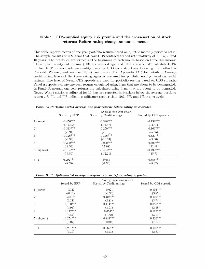
Table 9: CDS-implied equity risk premia and the cross-section of stockreturns: Before rating change announcements

This table reports means of one-year portfolio returns based on quintile monthly portfolio sorts.The sample consists of U.S. firms that have CDS contracts traded with maturity of 1, 3, 5, 7, and10 years. The portfolios are formed at the beginning of each month based on three dimensions:CDS-implied equity risk premia (ERP), credit ratings, and CDS spreads. We calculate CDS-implied ERP for each reference entity using its CDS term structures following the method inFriewald, Wagner, and Zechner (2014) (see Section 7 & Appendix IA.5 for details). Averagecredit rating levels of the three rating agencies are used for portfolio sorting based on creditratings. The level of 5-year CDS spreads are used for portfolio sorting based on CDS spreads.Panel A reports average one-year returns calculated using firms that are about to be downgraded.In Panel B, average one-year returns are calculated using firms that are about to be upgraded.Newey-West t-statistics adjusted for 11 lags are reported in brackets below the average portfolioreturns. *, **, and *** indicate significance greater than 10%, 5%, and 1%, respectively.

Panel A: Portfolio-sorted average one-year returns before rating downgrades

Average one-year returnSorted by ERP Sorted by Credit ratings Sorted by CDS spreads

1 (lowest) -0.456*** -0.386*** -0.139***(-17.95) (-11.47) (-4.84)

2 -0.333*** -0.250*** -0.169***(-8.94) (-8.16) (-5.55)

3 -0.326*** -0.366*** -0.320***(-8.33) (-10.33) (-9.30)

4 -0.302*** -0.290*** -0.405***(-8.53) (-7.98) (-12.19)

5 (highest) -0.164*** -0.454*** -0.492***(-3.59) (-12.21) (-15.73)

5−1 0.292*** -0.068 -0.353***(5.59) (-1.36) (-8.32)

Panel B: Portfolio-sorted average one-year returns before rating upgrades

Average one-year returnSorted by ERP Sorted by Credit ratings Sorted by CDS spreads

1 (lowest) -0.027 -0.021 0.103***(-0.61) (-0.30) (3.85)

2 0.083** 0.103*** 0.110***(2.21) (2.81) (3.74)

3 0.160*** 0.114*** 0.088***(4.97) (3.91) (2.58)

4 0.117*** 0.054** 0.102***(4.57) (1.82) (3.11)

5 (highest) 0.254*** 0.241*** 0.220***(9.07) (10.06) (7.10)

5−1 0.281*** 0.262*** 0.118***(5.39) (3.53) (2.87)

46

Appendix

Appendix A Variable Definitions

Rating-level variables

• dCDS is an indicator variable equal to one if the rating change takes place when the CDStrades on the underlying firm, and 0 otherwise.

• Previous Rating is the credit rating level prior to the rating change. It is expressed as thenatural logarithm of the cardinal rating scale; see Table B1 for the mapping

• Abs Rating Change is the absolute value of the difference in rating scale change between afterand before rating change events.

• Days Since Last Rating is the natural logarithm of the number of days between the previousrating change in the same direction for the same bond issue, but by another rating agency.Following Jorion, Liu, and Shi (2005), the number of days is set to 60 (a) if both rating agenciesrate on the same day, (b) if the rating by the second rating agency is in the opposite direction,or(c) if the rating change by the other rating agency is more than 60 days.

• Earnings Ann Related is an indicator variable equal to one if there is an earnings announcementwithin (-1,+1) days of the rating change event day, and 0 otherwise.

• dDowngrade is an indicator variable equal to one if the bond experiences a rating downgradeevent, and 0 otherwise.

Firm-level variables: Firm fundamentals

• Sales is the firm’s quarterly sales (saleq) reported in COMPUSTAT.

• Assets is the firms’ quarterly total assets (atq) reported in COMPUSTAT.

• Operating income is the quarterly operating income (oiadpq) reported in COMPUSTAT.

• Profitability is the firm’s quarterly ratio of Operating income to Sales.

• Total debt is the firm’s total debts (dlcq + dlttq) reported in the quarterly COMPUSTAT.

• Leverage is the firm’s Total debt divided by its Assets.

• Market value of equity is the market value of equity calculated using the monthly CRSPdatabase, i.e. share price × total shares outstanding.

• Book value of equity is the book value of equity. It is the total assets minus total liability plustax credit (atq−ltq + txditcq) calculated using quarterly COMPUSTAT.

• Mkt-to-Book is the monthly ratio of Market value of equity divided by the Book value of equity.

• Avg Volatility is the monthly standard deviation of daily stock returns caculated using datafrom CRSP.

• Avg Trading Volume is the monthly trading volume on the stock reported in CRSP.

• Avg Return is the monthly stock return obtained from CRSP.

47

Firm-level variables: CDS trading variables

• Analyst Coverage is the number of analyst EPS forecasts in the 90 days prior to the earningsannouncement date. (source: I/B/E/S)

• Analyst Dispersion is the standard deviation of analyst EPS estimates made in the 90 daysprior to the earnings announcement date scaled by the actual reported EPS. (source: I/B/E/S)

• Institutional Ownership is the ratio of total shares held by institutional investors to the totalshares outstanding for a given stock. (source: Thomson-Reuters Institutional Holdings (13F)Database)

• Stock Illiquidity is the monthly average stock illiquidity defined as the squared root of theAmihud (2002) measure. It is the monthly average of the following daily values where Rettand Pricet are daily return and price of the stock:

√1000000 ∗ |Rett|/ (Volume× Pricet).

• Bond Illiquidity is the number of outstanding bond issues in a given month (see Martin andZawadowski (2013)).

• Debt Outstanding is a proxy for hedging demand. It is the residual from regressing total amountdebt outstanding on the number of bond issues. In other words, this variable measures theamount of debt outstanding that is orthogonal to the number of bond issues.

• Forex Derivative Hedging is the average amount of foreign exchange derivatives used for hedgingpurposes (i.e. non-trading purposes) relative to total assets of the lead syndicate banks andbond underwriters that the firm has done business with in the past five years. Banks’ derivativesusage data is obtained from Bank Holding Company (BHC) Y9-C filings. Data on the firm’slead bank syndicate is obtained from LPC Dealscan, and the firm’s unwriter information isobtained from Mergent FISD.

CDS & Bond variables

• CDS Spread is the average monthly 5-year CDS spread from CMA and MARKIT databases.

• Bond Yield is the trade-weighted average monthly bond yield calculated from the TRACEdatabase.

• CDS Spread Change is the logarithmic difference in average monthly 5-year CDS spreads be-tween the current and previous months.

• Bond Yield Change is the logarithmic difference in trade-weighted average bond yields betweenthe current month and previous months.

• CDS Slope is the difference between the monthly average 10-year CDS spreads and the monthlyaverage 1-year CDS spreads.

• CDS-implied Rating Class is the firm’s credit rating class, on the scale of 1 to 6, that is backedout non-parametrically using CDS spreads. See Section 5.1 for more details.

• Credit Rating Class is the credit rating level mapped to the rating class scale. See TableAppendix B for the mapping.

48

• Credit watch dummy indicates whether the firm (or bond issue) is put on credit watch priorto a credit rating change. This monthly indicator variable takes the value 1 from the monthof the watch announcement to the month of the rating change event or until “Off Watch” or“Not On Watch” is announced. For downgrades, only negative watches are considered whilefor upgrades, only positive watches were considered. A credit watch announced 180 days ormore prior to when a firm is re-rated is not considered to be related to the rating changeevent. Credit watch data is obtained from Mergent FISD and Moody’s Default Risk Database(MDRS).

• Market Cap is the monthly market value of equity.

• Market Leverage is defined as (Total debt + Market value of equity)/(Market value of equity)calculated at a quarterly frequency.

• Long Term Debt-to-Asset is the ratio of long term debt to total assets (dlttq/atq) calculatedusing quarterly COMPUSTAT.

• ERP is the firm’s annualized equity risk premium implied by the dynamic of CDS term struc-ture.

• Subordinate is an indicator variable equal to one if the bond is subordinated. We obtain bondcharacteristics from Mergent FISD, CUSIP Master file, and Moody’s Default Risk Database(MDRS).

• Callable is an indicator variable equal to one if the bond is callable or redeemable, and zerootherwise.

• Issue Size is the offering amount of the bond at primary issue.

• Maturity is the maturity of the bond in years.

• Treasury Slope (10yr-1yr) is the difference between the 10-year and 1-year Treasury rates.

• Bond return is the raw bond return around the rating change event (t = 0) calculated over the[−k,+k] event days as:

BondReturnt=0 =BondPricet+k −BondPricet−k +AccruedInterest

BondPricet−k.

We use the shortest event window possible depending on the availability of bond trading history.The maximimum window of k = 7 days is used, otherwise bond event-period return is notcomputed.

• Daily bond index is the weighted (equal or value) index of bond returns grouped according toMoody’s six major rating categories.

Bankruptcy & Distress regression variables

• Bankruptcy is defined as when the firm experiences a credit default event as defined in Moody’sUltimate Recovery Database (Moody’s URD).

• Net Income-to-Assets is the ratio of net income to total assets (niq/atq) obtained from quarterlyCOMPUSTAT.

49

• Total Liabilities-to-Assets is the ratio of total liabilities to total assets (ltq/atq) obtained fromquarterly COMPUSTAT.

• Relative Size is the logarithmic of the firm’s market value of equity divided by the totalNYSE/AMEX market equity value. It is calculated monthly using data from CRSP.

• Excess Return is the monthly return on the firm minus the value-weighted NYSE/AMEX indexreturn.

50

Appendix B Additional Tables

Table B1: Classification of credit rating codes

The table presents the mapping of rating codes issued by S&P, Fitch, and Moody’s to the cardinal scale,as well as to the rating class. The rating codes used by S&P and Fitch are similar but are different fromthose used by Moody’s. Moody’s uses code from Aaa down to C to rate bonds whereas S&P and Fitchrate bonds from AAA down to D. Within the 6 classes from AA to CCC for S&P and Fitch, the ratingagencies have three additional gradations with modifiers (+,none,-). For examples, S&P’s AA rating classis subdivided into AA+, AA, AA-. Similarly, Moody’s has three additional gradations with modifiers1,2,3 from Aaa to Caa. We transformed the credit ratings of the three rating agencies into a cardinal scalestarting with 1 as AAA(Aaa), 2 as AA+(Aa1), 3 as AA(Aa2), and so on until 23 as the default category.The rating class mapping is from Jorion and Zhang (2007). Fitch differs from the other two agencies inthat it provides three ratings for default. We follow Jorion, Liu, and Shi (2005) by using 23 instead of 22as the cardinal scale for Fitch’s default category, which is the average of three default ratings – i.e., DD.

Description S&P Moody’s Fitch Cardinal scale Rating class

Investment gradeHighest grade AAA Aaa AAA 1 1High grade AA (+,none,-) Aa (1,2,3) AA (+,none,-) 2, 3, 4 1Upper-medium grade A (+,none,-) A (1,2,3) A (+,none,-) 5, 6, 7 2Medium grade BBB (+,none,-) Baa (1,2,3) BBB (+,none,-) 8, 9, 10 3Speculative gradeLower medium grade BB (+,none,-) Ba (1,2,3) BB (+,none,-) 11, 12, 13 4Speculative B (+,none,-) B (1,2,3) B (+,none,-) 14, 15, 16 5Poor standing CCC (+,none,-) Caa (1,2,3) CCC (+,none,-) 17, 18, 19 6Highly speculative CC Ca CC 20 6Lowest quality C C C 21 6In default D DDD/DD/D 23 6

51

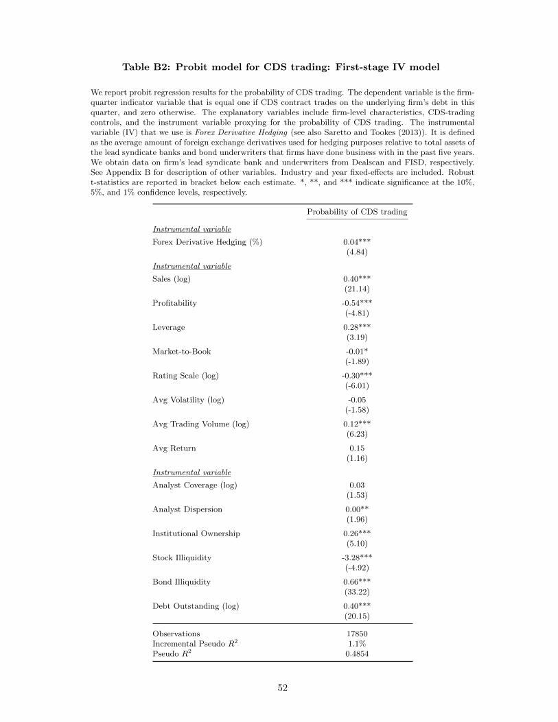
Table B2: Probit model for CDS trading: First-stage IV model

We report probit regression results for the probability of CDS trading. The dependent variable is the firm-quarter indicator variable that is equal one if CDS contract trades on the underlying firm’s debt in thisquarter, and zero otherwise. The explanatory variables include firm-level characteristics, CDS-tradingcontrols, and the instrument variable proxying for the probability of CDS trading. The instrumentalvariable (IV) that we use is Forex Derivative Hedging (see also Saretto and Tookes (2013)). It is definedas the average amount of foreign exchange derivatives used for hedging purposes relative to total assets ofthe lead syndicate banks and bond underwriters that firms have done business with in the past five years.We obtain data on firm’s lead syndicate bank and underwriters from Dealscan and FISD, respectively.See Appendix B for description of other variables. Industry and year fixed-effects are included. Robustt-statistics are reported in bracket below each estimate. *, **, and *** indicate significance at the 10%,5%, and 1% confidence levels, respectively.

Probability of CDS trading

Instrumental variable

Forex Derivative Hedging (%) 0.04***(4.84)

Instrumental variable

Sales (log) 0.40***(21.14)

Profitability -0.54***(-4.81)

Leverage 0.28***(3.19)

Market-to-Book -0.01*(-1.89)

Rating Scale (log) -0.30***(-6.01)

Avg Volatility (log) -0.05(-1.58)

Avg Trading Volume (log) 0.12***(6.23)

Avg Return 0.15(1.16)

Instrumental variable

Analyst Coverage (log) 0.03(1.53)

Analyst Dispersion 0.00**(1.96)

Institutional Ownership 0.26***(5.10)

Stock Illiquidity -3.28***(-4.92)

Bond Illiquidity 0.66***(33.22)

Debt Outstanding (log) 0.40***(20.15)

Observations 17850Incremental Pseudo R2 1.1%Pseudo R2 0.4854

52

Table B3: The propensity score matched sample

This table presents matched sample diagonoistics. All variables are defined in Appendix B. Panel Ashows the probit model used in the propensity score matching. We estimate firms’ probability of havingCDS trading in each month. The dependent variable in the probit model is the firm-month indicator thatis equal one if CDS contract trades on the underlying firm’s debt this month, and zero otherwise. Allindependent variables are lagged by one month. The first column in Panel A (Before matching) reportsresults estimated using the full sample for which data are available. The second column in Panel A (Aftermatching) reports results estimated using the CDS-traded and propensity-score matched firms. Firmsfor which CDS contracts trade at any point in our sample period (1996-2010) are identified with thetreatmeant group, i.e. traded-CDS firms. Firms in the control group used in the matching are thosein the full sample that never have CDS contracts traded at any point in our sample period , i.e. non-traded-CDS firms. Each traded-CDS firm (treatment firm) is matched with up to five non-traded-CDSfirms (control firms) based on their propensity scores of having CDS trading. Industry and year fixedeffects are included in the regressions. Robust t-statistics clustered at the firm level are reported inbracket. *, **, and *** indicate statistical confidence greater than 10%, 5%, and 1%, respectively. PanelB reports pairwise comparisons of the variables used for matching for the CDS treatment firms, and thematched control firms. Panel C reports industry distributions (Fama-French 12 classification) for theCDS treatment firms, and the matched control firms.

Panel A: Propensity score matched sample

Before matching After matching

Sales (log) 0.40*** 0.32***(36.44) (4.03)

Profitability -0.53*** -0.13(-8.14) (-0.25)

Leverage 0.26*** 0.14(5.05) (0.40)

Mkt-to-Book -0.01*** -0.01(-2.78) (-0.43)

Rating Scale (log) -0.26*** -0.72***(-9.10) (-3.61)

Avg Return 0.08 0.13(1.03) (1.11)

Avg Volatility (log) -0.06*** -0.06(-3.06) (-0.44)

Avg Trading Volume (log) 0.11*** -0.04(10.34) (-0.57)

Analyst Coverage (log) 0.03** -0.01(2.57) (-0.12)

Analyst Dispersion 0.00*** -0.00(3.66) (-0.38)

Institutional Ownership 0.26*** 0.07(8.76) (0.39)

Stock Illiquidity -3.27*** -3.55(-7.94) (-0.94)

Bond Illiquidity 0.66*** 0.10(56.56) (1.43)

Debt Outstanding (log) 0.40*** 0.16**(34.27) (2.21)

Forex Derivative Hedging (%) 0.04*** -0.11**(7.23) (-2.32)

Observations 52440 1011Pseudo R2 0.49 0.14

53

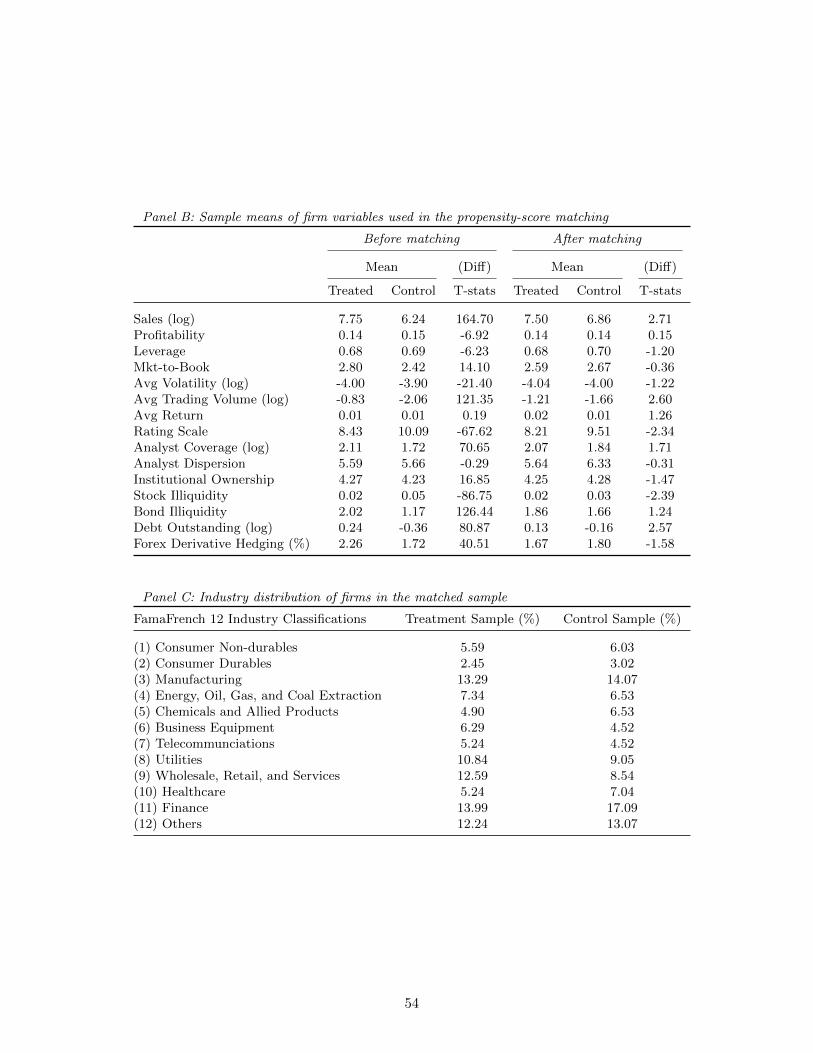
Panel B: Sample means of firm variables used in the propensity-score matching

Before matching After matching

Mean (Diff) Mean (Diff)

Treated Control T-stats Treated Control T-stats

Sales (log) 7.75 6.24 164.70 7.50 6.86 2.71Profitability 0.14 0.15 -6.92 0.14 0.14 0.15Leverage 0.68 0.69 -6.23 0.68 0.70 -1.20Mkt-to-Book 2.80 2.42 14.10 2.59 2.67 -0.36Avg Volatility (log) -4.00 -3.90 -21.40 -4.04 -4.00 -1.22Avg Trading Volume (log) -0.83 -2.06 121.35 -1.21 -1.66 2.60Avg Return 0.01 0.01 0.19 0.02 0.01 1.26Rating Scale 8.43 10.09 -67.62 8.21 9.51 -2.34Analyst Coverage (log) 2.11 1.72 70.65 2.07 1.84 1.71Analyst Dispersion 5.59 5.66 -0.29 5.64 6.33 -0.31Institutional Ownership 4.27 4.23 16.85 4.25 4.28 -1.47Stock Illiquidity 0.02 0.05 -86.75 0.02 0.03 -2.39Bond Illiquidity 2.02 1.17 126.44 1.86 1.66 1.24Debt Outstanding (log) 0.24 -0.36 80.87 0.13 -0.16 2.57Forex Derivative Hedging (%) 2.26 1.72 40.51 1.67 1.80 -1.58

Panel C: Industry distribution of firms in the matched sample

FamaFrench 12 Industry Classifications Treatment Sample (%) Control Sample (%)

(1) Consumer Non-durables 5.59 6.03(2) Consumer Durables 2.45 3.02(3) Manufacturing 13.29 14.07(4) Energy, Oil, Gas, and Coal Extraction 7.34 6.53(5) Chemicals and Allied Products 4.90 6.53(6) Business Equipment 6.29 4.52(7) Telecommunciations 5.24 4.52(8) Utilities 10.84 9.05(9) Wholesale, Retail, and Services 12.59 8.54(10) Healthcare 5.24 7.04(11) Finance 13.99 17.09(12) Others 12.24 13.07

54

Internet Appendix: Are credit ratings still relevant?

Sudheer Chava, Rohan Ganduri, and Chayawat Ornthanalai

This document contains discussions and additional results that were left out of the main paper dueto space considerations. We will be happy to include any of these findings in the main paper.

Appendix IA.1 Descriptives of the credit rating change sample

Panel A of Table IA1 summarizes the number of upgrades and downgrades along with the size oftheir rating changes over each year. There are about 2.1 downgrades for every upgrade, which ismore or less consistent with previous studies.25 We observe clustering of upgrades and downgrades incertain years over the 15-year period, and we find that 42% of all downgrades occurred in 2001-2002and 2007-2009, which correspond to the post-Internet bubble and the recent financial crisis periods,respectively. On the other hand, 39% of all upgrades occurred in pre-Internet bubble period, i.e.1997-1998, and when the market volatility level is historically low, i.e. 2006-2007, as measured bythe VIX index. The size of the rating change is the absolute value of the change in the ratingscale. The average size of the rating change does not vary significantly over the years. There are1416 downgrades and 689 upgrades during the period when the underlying firms have CDS contractstraded. On the other hand, there are 3249 downgrades and 1482 upgrades during the period whenthe underlying firms do not have CDS contracts traded. For downgrades (upgrades), the mean size ofthe absolute rating change for an issue without CDS trading is 1.69 (1.38), and for an issue with CDStrading, it is 1.55 (1.27). Table IA1 shows that the start dates of CDS trading in our sample begin in2001, when we observe only 12 downgrades on firms that have CDS contracts traded. Nevertheless,the number of firms that have CDS contracts traded increases significantly in subsequent years. Infact, Panel A shows that the numbers of downgrades on firms with and without CDS contracts tradedare roughly comparable after 2005.

In order to control for the differences between these two types of firms, we consider a subsampleof firms for which CDS starts trading at some point during our sample period. We refer to thissample as the “Traded-CDS”. Panel B of Table IA1 reports the sample size of traded-CDS sample.The average size of rating change for the sample is 1.45 before CDS trading starts and 1.49 afterCDS trading starts.

Table IA2 presents the distribution of the absolute magnitude of rating changes for the pre- andpost-CDS trading periods. Panel A reports the distribution year by year, while Panel B reports ab-solute rating changes for “within-letter-grade”, “across-letter-grade”, and “across-investment” ratingchanges. A rating change is defined as “within-letter-grade” if it is within the same alphabet let-ter (e.g., A+, A, A-). All other rating changes are classified as “across-letter-grade”. Among theacross-letter-grade changes, those that change between investment grade to speculative grade, andvice versa, are considered “ across-investment” grade changes. Table B1 in the appendix summarizesrating categories that belong to the investment and speculative grades.

Appendix IA.2 Other robustness tests for stock price reactions to rating changes

The abnormal returns of firms around credit rating events could be affected due to factors whichare unrelated to the rating event. In this case, the CARs would not average out to zero in the

25Our number is closer to that of Dichev and Piotroski (2001), who report twice as many downgrades as upgradesover their sample period of 1970 to 1987. In contrast, Jorion, Liu, and Shi (2005) report 4 downgrades for every upgradefrom 1998 to 2002.

1

cross-section. This problem can be alleviated by using standardized CAR (SCAR) instead of CAR.

We define SCAR as SCARi(−1,+1) = CARi(−1,+1)

σ(ARi)√

3, where σ(ARi) is the standard deviation of the

one-period mean abnormal return, and the factor of√

3 accounts for the length of the event window(-1,+1), which is equal to 3 days. We carry out all the univariate analysis, the regression analysis,and the matched sample analysis using SCAR instead of CAR as a measurement of abnormal returnsand obtain the same conclusions.

In order to rule out the possibility that our results are due to outliers, we winsorize each of theCAR and SCAR specifications at the 1% level. We also test for the difference in the mean of stockprice reactions between the pre- and post-CDS groups using bootstrapped standard errors. In bothcases, we find that the results do not change qualitatively. In addition, we conduct various othersubsample analyses based on credit rating agencies, industry type, across-investment-grade ratingchange, and we find that our results are robust.

We verify that our main conclusion holds for rating changes that are within-investment-grade,as well as those that are across investment grade. Using only traded-CDS firms, we find that stockprice reactions to rating downgrades in the pre-CDS-trading period is -1.72% for “within investmentgrade” rating changes, while it is -9.13% for “across investment grade ” rating changes. However, inthe post-CDS-trading period, we find that stock price reactions to rating downgrades is -0.84% and-2.86% for “within investment grade” and “across investment grade” rating changes, respectively. Inboth cases we find the difference in CAR(-1,1) to be positive and statistically different from zero.The difference in CARs between the pre-CDS-trading and post-CDS-trading periods for “withininvestment grade” rating change is 0.88% with a t-statistic of 1.82, while the for “across investmentgrade” rating change is 6.28% with a t-statistic of 3.60.

Apart from the instrumental variable analysis and the matched sample analysis described inSections 4.4–4.5, we apply the “placebo test” test to further rule out a concern that our results arerelated to changes in certain market conditions over time — e.g., changes in volatility. To do this,we first generate random pseudo CDS introduction dates. Then we apply the standard event studymethodology to these randomly generated pre- and post-CDS periods. We find that the differencein the stock price reactions between these pseudo pre- and post-CDS periods is not significantlydifferent from 0. Overall, using a host of robustness tests, we confirm that the abnormal stock returnaround credit rating downgrades is muted after CDS contracts trade on the underlying firm’s debt.

Appendix IA.3 Bond price reactions to rating changes

We examine the impact of the CDS market on corporate bond pricing as a channel through whichCDS trading attenuates firms’ equity price reactions to credit rating downgrades. The basic idea inthe cost of capital calculation is that the market value of the firm’s assets must equal the marketvalue of the firm’s debt plus the market value of the firm’s equity. Any impacts on the firm’s debtvalue can affect its equity return through changes in the firm’s total assets. We examine whetherbond prices also react less to credit rating downgrade announcements when firms have CDS tradingon their debt.

Similar to our analyses for stock returns, we consider a rating change event on a debt’s issueras one observation. We calculate the daily bond price using the trade-weighted average of all theprices reported during that day (see also Bessembinder, Kahle, Maxwell, and Xu (2009)). In anumber of cases, there are multiple bond issues per issuer. These multiple issues usually experiencerating changes on the same day. In order to avoid double counting events, we study the return of aweighted bond portfolio (equal or value weighted) for each firm. We construct both the equal- andvalue-weighted portfolios using all the issues written on a firm, and we find that the results are notqualitatively affected by the weighting methods. To save space, we present only the results that arebased on the value-weighted portfolios.

2

Unlike the stock sample analysis, bond trading is relatively thin. For instance, based on thefiltered sample in 2006–2007, we find that each bond issue, on average, trades on only 30 days peryear. Conditional on the day that we observe trades, there are approximately 3.48 trades per day. Tocompute abnormal bond returns, we follow the method advocated in Bessembinder, Kahle, Maxwell,and Xu (2009) by differencing the raw returns with the benchmark of indices. We match returnsto six benchmark indices based on Moody’s six major rating categories (Aaa, Aa, A, Baa, Ba, andB), and the equivalent S&P and Fitch rating categories (See the mapping in Appendix Table B1).Matching further on additional dimensions yields an inadequately small sample because the majorityof bonds do not trade daily. We construct daily bond return indices based on the above six ratingcategories. For each rating category, we calculate the daily index return using all of the bondsrated in that category. We exclude bonds that are re-rated on the day the index is constructed.Since few bonds trade on a daily basis, the composition of the index changes daily. As suggestedby Bessembinder, Kahle, Maxwell, and Xu (2009), the bond index return is computed using thevalue-weighted average to reflect the daily change in index composition.

The cumulative bond return is first calculated at the issue level using transaction prices observedimmidately before and after the event day. Because bonds do not often trade daily, the closestobservations to the event day may be several days away. We pick the closest pre-event and post-event bond trades around the event day (Day 0) in the (-7,+7) event window. If we do not observebond trades within (-7,+7) days relative to the event date, the rating change observation is excluded.On average, the closest transaction prices are observed on event-days -2.7 and +2.4 relative to theevent date.26 The cumulative abnormal return for the bond price is calculated by subtracting thecumulative bond return with the cumulative bond index return over the same window period. Finally,the bond market reaction to a rating change event for a firm is calculated as the value-weightedaverage returns of all of the issues traded around the event date.

Appendix Table IA7 displays the number of upgrades and downgrades and the sizes of ratingchanges per year in the bond sample. There are about twice the downgrades for every upgrade inthe bond event-study sample, which is similar to the stock sample (Table IA7). Relative to the stocksample, we find significantly fewer rating events. This is because TRACE and NAICS databaseshad limited bond coverage during the early years. We rely on NAICS bond database before 2002,which reports only bond trades executed by national insurance companies. For TRACE, it was notuntil March 2003 that it began to cover all the bonds with an issue size of at least $100 million thatwere rated “A” or higher. Nevertheless, in subsequent years, the coverage has steadily increased.The Traded-CDS sample for bonds is constructed in the same manner as for the stocks. Panel B ofTable IA7 shows a large reduction in the number of observations from the Full sample to the Traded-CDS sample. The number of unique firms in the Traded-CDS sample is only 123 (as opposed to 672unique firms for the full sample) Therefore, we rely mainly on the Full sample when interpreting theresults.

Table IA8 reports the mean bond cumulative abnormal returns (CAR) for the pre- and post-CDStrading periods. The results in Panel A are based on the full sample. Consistent with prior literature(Hand, Holthausen, and Leftwich (1992)), we find that bond prices react significantly to downgrades(-2.39%) but little to upgrades (0.0%). We find that average bond price reactions to rating upgradesin the post-CDS period is negative, but not significant. Panel A shows the mean of bond CARs todowngrades are negative and significant at the 1% level for both pre-CDS and post-CDS periods.However, the magnitude of bond price reaction is significantly weaker in the post-CDS period. Themean CARs for the pre- and post-CDS cases are -3.37% and -1.44%, respectively, and their differenceis significant at the 1% level. To rule out concerns that our results are due to outliers, we verify that

26Sampling over smaller event windows such as (-3,+3) and (-5,+5) lead to a very small sample of unique firms. Onthe other hand, extending the sampling window – e.g., (-15,+15) would increase the bias due to confounding informationarrivals (see Shivakumar, Urcan, Vasvari, and Zhang (2010), and Elkamhi, Jacobs, Langlois, and Ornthanalai (2011)).

3

the difference in the means of bond CARs to rating downgrades is statistically significant using thebootstrapped standard error. As for upgrades, the difference between bond price reactions in thepre- and post-CDS cases is not significant. This set of results is consistent with our findings on stockprice reactions to rating change announcements.

Panel B of Table IA8 displays results for the Traded-CDS sample, which represents firms thathave CDS traded at some point during 1996–2010. Again, we find that the overall bond price reactionto downgrades is negative (-1.91%) and significant at the 1% level. Consistent with our hypothesis,the magnitude of the bond price reaction is weaker in the post-CDS period (-1.61%) than in thepre-CDS period (-2.61%), although not significant. The fall in statistical power is clearly due to thesmall sample size. Also, most of the post-CDS downgrades for the bond sample occurs during thecrisis, i.e. 2007-2009, which could systematically amplify the magnitude of bond price reaction torating downgrade announcements.

Appendix IA.4 Primary market bond yields

This section tests whether CDS spreads are useful relative to credit ratings in explaining the primarymarket bond yields. Table IA6 reports the cross-sectional regression results where the dependentvariables are corporate bond yields, in basis points, observed at their primary bond issuance. Wereport results for four regression specifications. We include rating-level, firm-level, and bond-issuance-level controls in the regressions. Where appropriate, the control variables are lagged by one period.Industry, year, and rating agency fixed-effects are also included. Appendix B describes the controlvariables. We use lagged CDS quotes that are traded immediately prior to the bond issuance inorder to avoid the endogeneity concern that bond yields and CDS spreads are jointly determined.

In regression models (I) and (II), we compare the relative explanatory power of Credit Rating andCDS Spread to explain the cross section of primary market bond yields. Credit Rating is expressedon the cardinal scale (see Table B1 for mapping), and CDS Spread is expressed in basis points.The coefficient on Credit Rating in regression model (I) is 17.18 and significant at the one percentlevel, suggesting that credit ratings are useful for explaining the cross-section of newly issued bondyields. However, we find that once CDS Spread is introduced as a variable in the regression (seeregression model (II)), the size of coefficient on Credit Rating decreases by a third to 6.18. Wealso find a substantial increase in adjusted R2 when CDS Spread is added to the list of explantoryvariables —from 58.3 to 71.5 percent. We conclude that CDS spreads significantly help explain thecross-sectional variations in primary market bond yields in addition to credit ratings.

Because the Credit Rating variable is discrete while the CDS Spread is a continuous variable,we facilitate their comparison by expressing them as credit rating classes, which range from 1 to6. The mapping between credit rating scales to credit rating classes is shown in Table B1. ForCDS spreads, we use the CDS-implied rating classes calculated non-parametrically in Section 5.1.Regression models (III) and (IV) in Table IA6 report results where both CDS spreads and creditratings are converted to the same unit of measurement, i.e., credit rating classes. We find thatthe results remain qualitatively similar when using rating classes to define credit ratings and CDSspreads. There is a substantial increase in adjusted R2 when CDS-implied rating classe is addedto the list of explantory variables – from 57.9 percent in regression model (III) to 71.1 percent inregression model (IV). Overall, we find that CDS spreads provide incremental information for thepricing of primary market bond issuance.

Appendix IA.5 CDS-implied equity risk premia

This Appendix section describes how we empirically estimate the equity risk premia implied fromCDS spreads as shown in equation (18) of the main paper. For convenience, we replicate the equation

4

below

ERP Tt+τ ≡ −

logEPt

[STt+τ

]− logEQ

t

[STt+τ

]√∫ t+τt σ2

S,udu

·√∫ t+τ

tσ2E,udu, (19)

The equation above shows that calculating implied equity premium requires evaluating the Q- andP-measure expectations of future T -year CDS spreads. The expected risk-neutral CDS spreads canbe represented using the firm’s forward CDS spread, logEQ

t

[STt+τ

]= F τ×Tt , where F τ×Tt is the

forward T -year CDS spread contracted at time t for delivery at time t+ τ .As a result, we can write the CDS Sharpe ratio in equation (19) as

SRt+τ =logEP

t

[STt+τ

]− F τ×Tt√∫ t+τ

t σ2S,udu

. (20)

Relying on the established approach in Cochrane and Piazzesi (2005) who estimated bond risk premiausing the term structure of forward rates, Friewald, Wagner, and Zechner (2014) suggest that CDSSharpe ratio in equation (20) can be estimated from the term structure of forward CDS spreads forcontracts with maturities Tk ∈ T = {1, 3, 5, 7} ,

SRt+τ =1

4

∑Tk∈T

logSTkt+τ − Fτ×Tkt

SDt+τ,

where SDt+τ refers to the sample standard deviation of daily CDS spread returns between t andt+ τ. The above method yields time-series of CDS Sharpe ratio estimated from daily cross-maturityCDS spreads and CDS forward spreads. In order to extract the common component similar to that inCochrane and Piazzesi (2005), we regress daily time-series of SRt+τ on Ft =

(1, S1

t , F3×1t , F 5×1

t , F 7×1t

),

a vector of one-year CDS spread and one-year CDS forward spreads that start in 1, 3, 5, and 7 years.That is, we estimate

SRt+τ = γ′ · Ft + εt+τ . (21)

The fitted value of the estimated Sharpe ratio is then used for the implied equity premium calculation,which according to equation (18), is given by

ERP t+τ = −γ · FtσE,t,τ , (22)

where σE,t,τ denotes the time-t conditional equity volatility estimated as the sample standard devi-ation of daily equity returns from t− τ to t.

For our empirical analysis, we estimate one-year CDS-implied equity risk premium in equation(22) on a daily basis for each firm in the sample. We use a one-year estimation window in the

regression model (21) to obtain ERP t+τ with τ equal to one year. In order for firms to be eligible

for the ERP t+τ calculation, it must have sufficient data on CDS quotes at maturities 1, 3, 5, 7, and10 years.

Table IA9 reports results from constructing monthly portfolio sorts based on CDS-implied equityrisk premia (ERP). In Panel A, we report the mean characteristics of quintile sorted portfolios thatare formed monthly based on ERP. The means of portfolio characteristics are calculated using equalweights. Because the start dates of CDS trading differ across firms, the number of firms availablein monthly cross-sections also varies, but mostly increase from 2001 through 2010. On average,there are 72 firms available for quintile portfolio sorting each month. Panel A of Table IA9 showsno monotonic pattern in portfolio characteristics sorted based on CDS-implied equity premia. The

5

equity risk premia estimated from CDS spreads are not related to firms’ size or market-to-bookvalues. We also do not find that ERP monotonically explains firms’ cross-sections of credit ratings,as well as CDS spread levels.

Panel B of Table IA9 reports average one-year return of five portfolios sorted monthly based onERP, credit ratings, and CDS spreads. We assign equal weight to firms in each porfoltio. We find aclear and distinct monotonic pattern in equity returns across the five portfolios. Firms with higherequity risk premia implied by their CDS spreads earn higher returns, consistent with the predictionof structural models, e.g. Merton (1974). The difference in one-year average returns between thehighest (5) and lowest (1) ERP portfolios is economically large, with the magnitude of about 24%per year. The t-statistic associated with this magnitude is 13.0, suggesting an overwhelmingly strongstatistical significance. Friewald, Wagner, and Zechner (2014) find the difference between the highestand lowest portfolios sorted by one-month ERP is about 1.51% per month after the risk-free rate(i.e., 18.12% per year). Thus, our results are roughly in line with theirs.

Panel B also shows that average one-year returns of portfolios sorted monthly based on creditratings and CDS spreads do not monotonically explain the cross-section of equity returns. Sortingportfolios based on credit rating scales result in a 7.1% difference in average one-year returns betweenthe worst-rated (5) and best-rated (1) firms. The finding is much weaker when we sort portfoliosbased on the level of CDS spreads. We do not find any significant difference in one-year portfolioreturns between the highest (5) and lowest (1) CDS spread firms. Overall, Panel B shows thatERP estimated from CDS term structures are informative of equity returns, while the level of CDSspreads alone are not. Further, the findings suggest that ratings issued by credit rating agencies arenot a good measure of default risk premium, and hence cannot explain cross-section of equity returnsequally well relative to the ERP estimated from CDS spreads.

6

Table IA1: Distribution of bond rating changes

The sample consists of 4,665 downgrades and 2,171 upgrades of taxable corporate bonds issued by U.S.firms from January 1996 to December 2010. The sample is split between rating changes that occur in thepresence of CDS trading (post-CDS period) and in the absence of CDS trading (pre-CDS period) on theunderlying firm’s debts. Panel A reports year-by-year distribution of rating changes. Count representsthe number of rating changes. Size represents the mean of the cardinal value of the new rating minus thecardinal value of the old rating. Bond ratings are converted to a cardinal scale measured on a 23-pointscale (see Appendix A for the mapping). Panel B reports the number of rating changes and the averagesizes of rating changes for the “Full Sample” and the “Traded-CDS”. The full sample represents the entiresample period consisting of firms that have and do not have CDS traded on their debts. Traded-CDSsample consists only of firms that have CDS trading at any point in our sample period, i.e from 1996 to2010.

Panel A: Distribution of number and size of bond rating changes by year

Downgrades Upgrades

Year Pre-CDS Post-CDS Pre-CDS Post-CDS

Count Size Count Size Count Size Count Size

1996 16 1.31 31 1.231997 149 1.39 206 1.351998 251 1.65 195 1.521999 310 1.63 147 1.232000 428 1.73 128 1.342001 556 1.92 12 1.25 99 1.422002 510 1.74 72 1.25 66 1.45 4 1.002003 226 1.76 109 1.25 85 1.47 20 1.052004 131 1.63 108 1.31 97 1.33 73 1.252005 110 1.49 128 1.59 71 1.76 95 1.252006 98 1.23 170 1.60 95 1.22 132 1.172007 101 1.60 181 1.56 81 1.26 134 1.222008 112 1.56 290 1.62 58 1.24 77 1.312009 178 1.70 258 1.83 35 1.57 43 1.812010 73 1.42 88 1.27 88 1.38 111 1.28

Total 3249 1.69 1416 1.55 1482 1.38 689 1.27

Panel B: Distribution of number and size of bond rating changes by sub-sample

Downgrades Upgrades

Sample Pre-CDS Post-CDS Pre-CDS Post-CDS

Count Size Count Size Count Size Count Size

Full sample 3249 1.69 1416 1.55 1482 1.38 689 1.27Traded-CDS sample 803 1.45 1029 1.49 300 1.22 574 1.29

7

Table IA2: Sample distribution by magnitude of rating changes

The sample consists of 4,665 downgrades and 2,171 upgrades of taxable corporate bonds issued by U.S.firms from January 1996 to December 2010. The sample is split between rating changes that occur inthe presence of CDS trading (post-CDS period) and in the absence of CDS trading (pre-CDS period) onthe underlying firm’s debts. In Panel A, Freq represents the number of rating changes. Bond ratingsare converted to a cardinal scale measured on a 23-point scale. Scale change represents the absolutechange, in cardinal value, of the new rating minus the old rating. Pct represents the percentage of ratingchanges observed in each scale change group. Panel B reports the distribution of rating changes for threerating-change classifications. A rating change is classified as “Within letter grade” if it is within the sameletter group (e.g., A+, A, A-). All other rating change events are classified as “Across letter grade” astheir change is from one letter group to a different letter group. We classify a rating change as“AcrossInv Grade” if the change is from an investment grade to a speculative grade or vice-versa. Investmentgrade rating for S&P and Fitch corresponds to rating levels of BBB and above. Investment-grade ratingfor Moody’s corresponds to rating levels of Baa and above.

Panel A: Sample distribution by absolute magnitude of rating changes

Downgrades Upgrades

Scale change Pre-CDS Post-CDS Pre-CDS Post-CDS

Freq Pct(%) Freq Pct(%) Freq Pct(%) Freq Pct(%)

1 1945 59.86 979 69.14 1168 78.81 557 80.842 802 24.68 272 19.21 206 13.90 102 14.803 299 9.20 82 5.79 56 3.78 19 2.764 106 3.26 39 2.75 26 1.75 4 0.585 42 1.29 22 1.55 7 0.47 5 0.736 20 0.62 10 0.71 5 0.347 15 0.46 7 0.49 5 0.348 10 0.31 2 0.14 1 0.07 2 0.299 5 0.15 2 0.1310 3 0.09 1 0.0711 2 0.06 2 0.14 3 0.2012 1 0.0714 1 0.07 1 0.07

Total 3249 100.00 1416 100.00 1482 100.00 689 100.00

Panel B: Sample distribution within and across rating

Downgrades Upgrades

Pre-CDS Post-CDS Pre-CDS Post-CDS

Freq Pct(%) Freq Pct(%) Freq Pct(%) Freq Pct(%)

Within letter grade 1714 52.75 655 46.26 592 39.95 258 37.45Across letter grade 1535 47.25 761 53.74 890 60.05 431 62.55Across Inv grade 367 11.30 206 14.55 167 11.27 79 11.47

8

Table IA3: Stock price reactions to bond rating changes: Robustness I

This table reports regression results of stock price reactions to bond rating changes. Thesample consists of credit rating change events on taxable corporate bonds issued by U.S.firms from January 1996 to December 2010. The dependent variable is the cumulativeabnormal return (CAR) calculated over the 3-day event window (-1,+1) using the marketmodel. Panel A consists of the full sample and includes Industry×Year fixed effects tocontrol for time-varying industry-level fixed effects. Panel B consists of only non-financialfirms. All the variables are defined in Appendix A. dCDS is an indicator variable equal toone when the firm has CDS contracts traded on its debt, and zero otherwise. Coefficientson other controls have been omitted to conserve space. Robust t-statistics are clusteredat the firm-level and reported in brackets below each estimate. *, **, and *** indicatesignificance at the 10%, 5%, and 1% confidence levels, respectively.

Panel A: Time-varying industry-level FE

Downgrades Upgrades

Full sample Full sample

(I) (I)

dCDS 1.25* 0.14(1.80) (0.53)

Rating controls X XFirm controls X XCDS-trading controls X X

Fixed effects Ind×Year Ind×YearObservations 4176 1972Adjusted R2 0.126 0.009

Panel B: Non-financial firms

Downgrades Upgrades

Full sample Traded-CDS Full sample Traded-CDS

(I) (II) (III) (IV) (I) (II) (III) (IV)

dCDS 2.61*** 1.80** 1.53** 2.62*** -0.34 -0.11 -0.04 -0.14(4.35) (2.44) (2.45) (3.75) (-1.40) (-0.44) (-0.14) (-0.33)

Rating controls X X X X X X X XFirm controls X X X X X X X XCDS-trading controls X X X X X X X X

Fixed effects Ind Ind & Year Ind ×Year Ind Ind Ind & Year Ind ×Year IndObservations 3333 3333 3333 1559 1623 1623 1623 729Adjusted R2 0.126 0.129 0.136 0.082 0.001 -0.004 0.010 -0.004

9

Table IA4: Stock price reactions to bond rating changes: Robustness II

This table reports regression results of stock price reactions to bond rating changes. Thesample consists of credit rating change events on taxable corporate bonds issued by U.S.firms from January 1996 to December 2010. In Panel A the dependent variable is thecumulative abnormal return (CAR) calculated over the 3-day event window (-1,+1) usingthe Fama-French 3 factor model. In Panel B the dependent variable is the cumulativeabnormal return (CAR) calculated over the 3-day event window (-1,+1) using the marketmodel. All the variables are defined in Appendix A. dCDS is an indicator variable equalto one when the firm has CDS contracts traded on its debt, and zero otherwise. In Panel BdDowngrade is an indicator variable equal to one if the rating change is a downgrade, andzero for an upgrade. We also interact all rating controls with dDowngrade. Coefficientson other controls have been omitted to conserve space. Robust t-statistics are clusteredat the firm-level and reported in brackets below each estimate. *, **, and *** indicatesignificance at the 10%, 5%, and 1% confidence levels, respectively.

Panel A: Fama-French 3 factor adjusted CAR

Downgrades Upgrades

Full sample Traded-CDS Full sample Traded-CDS

(I) (II) (III) (IV) (I) (II) (III) (IV)

dCDS 1.86*** 1.52** 1.12* 2.29*** -0.17 -0.06 0.04 0.05(3.09) (2.18) (1.69) (3.36) (-0.74) (-0.22) (0.15) (0.12)

Rating controls X X X X X X X XFirm controls X X X X X X X XCDS-trading controls X X X X X X X X

Fixed effects Ind Ind & Year Ind ×Year Ind Ind Ind & Year Ind ×Year IndObservations 4176 4176 4176 1775 1972 1972 1972 834Adjusted R2 0.123 0.124 0.127 0.092 0.002 0.003 0.017 -0.001

Panel B: Pooled Downgrades & Upgrades

Full sample Traded-CDS

(I) (II) (III) (IV)

dCDS×dDowngrade 1.61*** 1.65*** 1.48** 1.38*(2.70) (2.81) (2.56) (1.83)

dDowngrade -3.23*** -3.30*** -3.09*** -3.13***(-8.51) (-8.14) (-7.16) (-4.29)

dCDS 0.28 0.05 -0.18 0.88(0.76) (0.13) (-0.44) (1.62)

Rating controls X X X XFirm controls X X X XCDS-trading controls X X X X

Fixed effects Ind Ind & Year Ind ×Year IndObservations 6148 6148 6148 2609Adjusted R2 0.133 0.134 0.138 0.091

10

Table IA5: Diff-in-diff downgrade CAR regression: 1–to–1 matchingwithout replacement

This table reports diff-in-diff regression analysis of stock price response CAR(-1,1) to bonddowngrades for the propensity-score matched sample. One non-traded-CDS (control)firm is matched to one traded-CDS (treated) firm without replacement. The caliper andcommon support conditions are not imposed for this 1:1 matching exercise. Panel Areports the main diff-in-diff regression results for the matched sample. Panel B reportsmatching diagnostics via a probit regression before and after matching. All the variablesare defined in Appendix A. Coefficients on other controls have been omitted to conservespace. Robust t-statistics clustered at the firm-level and are reported in bracket beloweach estimate. *, **, and *** indicate significance at the 10%, 5%, and 1% confidencelevels, respectively.

Panel A: 1:1 Matched Sample

Diff-in-diff Subsamples (diagnostics)

Treatment Control Post-CDS Pre-CDS

(I) (II) (III) (IV) (V) (VI)

dTreatment×dCDS 2.50*** 2.42***(2.64) (2.63)

dCDS -0.79 -1.78 1.91** -1.03(-0.95) (-1.59) (2.45) (-1.25)

dTreatment -0.09 -0.29 2.12** 0.17(-0.11) (-0.39) (2.29) (0.19)

Rating controls X X X X X XFirm controls X X X X X XCDS-trading controls X X X X X X

Fixed effects Ind Ind & Year Ind Ind Ind IndObservations 2883 2883 1797 1086 1753 1130Adjusted R2 0.097 0.099 0.087 0.109 0.105 0.103

Panel B: 1:1 Matching Diagnostics via Probit Regression

Before matching After matching Before matching After matching

Sales (log) 0.40*** 0.48*** Analyst Coverage (log) 0.03** 0.29**-36.44 -5.43 -2.57 -2.51

Profitability -0.53*** 1.39 Analyst Dispersion 0.00*** 0(-8.14) -1.49 -3.66 -0.87

Leverage 0.26*** 0.45 Institutional Ownership 0.26*** 0.29-5.05 -0.68 -8.76 -0.87

Market-to-Book -0.01*** 0.02 Stock Illiquidity -3.27*** -2.13*(-2.78) -0.54 (-7.94) (-1.79)

Rating Scale (log) -0.26*** -0.84** Bond Illiquidity 0.66*** 1.14***(-9.10) (-2.09) -56.56 -7.01

Avg Return 0.08 1.08* Debt Outstanding (log) 0.40*** 0.72***-1.03 -1.72 -34.27 -4.66

Avg Volatility (log) -0.06*** 0.4 Forex Derivative Hedging (%) 0.04*** 0.00(-3.06) -1.45 -7.23 -0.02

Avg Trading Volume (log) 0.11*** -0.02-10.34 (-0.15)

Observations 52440 484Pseudo R2 0.49 0.60

11

Table IA6: Primary market bond yields regression

This table reports regression results for the determinants of primary market bond yields. The sampleconsists of coporate bonds issued by firms that have CDS contracts trading on their debt. The dependentvariables are corporate bond yield spreads (in bps) observed at issuance. Regression models (I) and (II)examine the explanatory power of credit rating levels and lagged CDS spreads. Credit Rating is the ratinglevel, in cardinal scale, issued by the credit rating agency. CDS Spread is the firm’s 5-year CDS spread (inbps) last observed prior to the bond issuance date. In regression models (III) and (IV), credit rating andCDS-implied rating are expressed as rating class, i.e. between 1 to 6; see Table B1 for mapping. CDS-implied rating class is calculated using the nonparametric method described in Section 5.2. We includevarious issuance-level and firm-level controls in the regressions. Subordinate is an indicator variable equalto one if the issued bond is a subordinate debt, and zero otherwise. Callable is an indicator variable equalto one if the issued bond has a callable option. Issue Size is the log of the notational amount (in $) ofthe bonds issued. Maturity is the maturity of the issued bond. Firm-level characteristics are calculatedusing information in the quarter prior to bond issuance; see Appendix B for details. Treasury Slope is thedifference between 10-year and 1-year treasury yields. All regressions include industry, year, and ratingagency fixed-effects. Robust t-statistics are clustered at the firm level and reported in parentheses. *, **,and *** indicate significance at the 10%, 5%, and 1% confidence levels, respectively.

Dependent variable: Primary market bond yields (bps)

(I) (II) (III) (IV)

Credit Rating (cardinal scale) 17.18*** 6.18***(9.84) (4.57)

CDS Spread (bps) 0.58***(9.91)

Credit Rating class 49.23*** 12.76***(9.13) (2.97)

CDS-implied Rating class 56.34***(15.51)

Issuance-level controls

Subordinated 23.66** 23.87*** 21.44** 25.61***(2.30) (3.10) (2.21) (3.19)

Callable -3.83 -0.42 -1.57 -1.23(-0.52) (-0.07) (-0.21) (-0.20)

Issue Size (log) 51.16*** 48.86*** 49.99*** 46.89***(5.40) (4.89) (5.37) (5.27)

Maturity (yrs) 0.87*** 1.09*** 0.90*** 1.17***(3.70) (5.77) (3.92) (5.62)

Other controls

Sales (log) -19.57*** -21.89*** -19.13*** -21.04***(-4.24) (-5.30) (-4.06) (-5.41)

Profitability -17.88 -11.96 -21.07 -18.18*(-1.49) (-1.05) (-1.62) (-1.75)

Long-Term Debt-to-Assets 8.89 -43.01 7.69 -43.84(0.27) (-1.55) (0.24) (-1.61)

Leverage 0.83 -1.89 0.48 -2.59**(0.65) (-1.57) (0.36) (-2.16)

Treasury Slope (10yr-1yr) 5.02 1.43 7.17 3.05(0.68) (0.21) (0.98) (0.46)

Rating-type FE Yes Yes Yes YesIndustry FE Yes Yes Yes YesYear FE Yes Yes Yes Yes

Observations 2208 2208 2208 2208Adj. R2 0.583 0.715 0.579 0.711

12

Table IA7: Distribution of bond rating changes: Bond market reaction sample

We report the distribution of bond rating change events used in the bond market reaction analysis.The full sample consists of 2,336 downgrades and 1,019 upgrades of taxable corporate bonds issuedby U.S. firms from January 1996 to December 2010. The sample is split between rating changesthat occur in the presence of CDS trading (post-CDS period), and in the absence of CDS trading(pre-CDS period) on the underlying firm’s debts. Panel A reports year-by-year distribution ofrating changes. Count represents the number of rating changes. Size represents the mean of thecardinal value of the new rating minus the cardinal value of the old rating. Bond ratings areconverted to a cardinal scale measured on a 23-point scale (see Table B1 for the mapping). PanelB reports the number of rating changes and the average sizes of rating changes for the “FullSample” and the “Traded-CDS”. The full sample represents the entire sample period consistingof firms that have and do not have CDS traded on their debts. Traded-CDS sample consists onlyof firms that have CDS trading at any point in our sample period, i.e from 1996 to 2010.

Panel A: Distribution of number and size of bond rating changes by year

Downgrades Upgrades

Year Pre-CDS Post-CDS Pre-CDS Post-CDS

Count Size Count Size Count Size Count Size

1996 3 1.00 2 1.001997 8 1.25 16 1.311998 22 1.50 23 1.351999 35 1.43 21 1.142000 71 2.15 17 1.822001 140 2.31 11 1.18 29 1.972002 208 1.96 47 1.26 16 1.19 3 1.002003 94 1.93 83 1.22 32 1.41 15 1.072004 48 1.56 92 1.33 40 1.40 38 1.162005 81 1.65 122 1.64 43 1.67 74 1.262006 71 1.38 164 1.80 82 1.48 133 1.112007 79 1.59 151 1.74 64 1.69 130 1.222008 95 1.48 240 1.66 32 2.69 70 1.692009 160 1.87 244 1.70 33 2.18 53 2.512010 36 1.44 31 1.23 16 1.25 37 1.59

Total 1151 1.81 1185 1.61 466 1.64 553 1.40

Panel B: Distribution of number and size of bond rating changes by sub-sample

Downgrades Upgrades

Sample Pre-CDS Post-CDS Pre-CDS Post-CDS

Count Size Count Size Count Size Count Size

Full sample 1151 1.81 1185 1.61 466 1.64 553 1.40Traded-CDS sample 237 1.48 465 1.58 55 1.09 296 1.35

13

Table IA8: Bond price response to credit rating downgrades and upgrades

This table reports cumulative abnormal returns (CAR) of bond price to credit rating downgradesand upgrades.The full sample consists of 2,336 downgrades and 1,019 upgrades of taxable corpo-rate bonds issued by U.S. firms from January 1996 to December 2010. Table IA7 in the appendixreports the distribution of bond rating changes used in this analysis. Panel A reports results forthe full sample, while Panel B reports results for the traded-CDS sample. The traded-CDS sample(Panel B) consists only of firms that have CDS trading at any points in our sample period. Ineach panel, the sample is split between rating changes that occur in the presence of CDS trading(Post-CDS period) and in the absence of CDS trading (Pre-CDS period) on the underlying firm’sdebts. Cumulative abnormal bond return is defined as the firm’s value-weighted bond portfolio’sexcess return against the bond return of a matching portfolio based on Moody’s six major ratingcategories (Aaa, Aa, A, Baa, Ba, and B). The event window is the shortest trading window within(-7,+7) calendar days relative to the rating change event day. T-statistics are displayed in squarebrackets. *, **, and *** indicate significance greater than 10%, 5%, and 1%, respectively.

Panel A: Full sample

Downgrades Upgrades

Mean CAR(%) Count Mean CAR(%) Count

Pre-CDS -3.37*** 1151 0.12 466(-10.25) (1.11)

Post-CDS -1.44*** 1185 -0.11 553(-4.44) (-1.10)

Difference (Pre–Post) 1.93*** -0.23(4.18) (-1.57)

Total -2.39*** 2336 -0.00 1019(-10.32) (-0.06)

Panel B: Traded-CDS sample

Downgrades Upgrades

Mean CAR(%) Count Mean CAR(%) Count

Pre-CDS -2.61*** 237 0.09 55(-4.01) (0.26)

Post-CDS -1.61*** 465 -0.25** 296(-3.46) (-1.74)

Difference (Pre–Post) 1.00 -0.34(1.25) (-0.93)

Total -1.94*** 702 -0.20 351(-5.14) (-1.49)

14

Table IA9: CDS-implied equity risk premium and portfolio characteristics

This table reports means of portfolio characteristics and one-year average portfolio returns sortedby CDS-implied equity risk premia (ERP). The sample consists of U.S. firms that have CDS con-tracts with maturity of 1, 3, 5, 7, 10 years trading on their debts. We calculate daily CDS-impliedERP with one-year horizon for each reference entity using its CDS term structure. We followthe method in Friewald, Wagner, and Zechner (2014) for calculating ERP, which is motivated byCochrane and Piazzesi (2005) who estimated bond risk premia using the term structure of forwardrates. Section 7 describes the procedure for calculating ERP. In Panel A, we report the meancharacteristics of quintile sort portfolios that are formed monthly based on based on CDS-impliedERP. The means of portfolio characteristics are calculated using equal weights and the sorting isdone at the beginning of each month. Because the start dates of CDS trading differ across firms,the number of firms available in monthly cross-sections also varies, but mostly increase from 2001through 2010. We require a minimum of 20 firms in the cross section to execute the portfoliosorts. Size is the log of firm’s market capitalization. Mkt-to-Book is the ratio of a firm’s marketvalue of total assets to its book value of total assets. Credit rating is the average firm’s creditratings, in cardinal scale, given by the three agencies: Moody’s, Fitch, and S&P. CDS spread isthe 5-year CDS spread level of the firm. In Panel B, we report average one-year equity returnsof portfolios sorted monthly based on ERP, credit ratings, and CDS spreads. The fifth (highest)quintile portfolio corresponds to firms with the highest ERP, lowest-rated firms, and largest CDSspreads. Newey-West t-statistics adjusted for 11 lags are reported in brackets below the averageportfolio returns in Panels B–C. *, **, and *** indicate significance greater than 10%, 5%, and1%, respectively.

Panel A: Portfolio characteristics sorted by CDS-implied ERP

Average valuesERP Size Mkt-to-Book Credit rating CDS spread

1 (lowest ERP) -0.005 15.753 2.486 9.105 0.0152 0.005 21.289 2.931 7.913 0.0063 0.009 22.842 2.806 8.151 0.0074 0.016 18.925 2.635 8.739 0.0115 (highest ERP) 0.034 12.095 2.392 10.016 0.025

Panel B: Average one-year returns of single-sorted portfolios

Average one-year returnSorted by ERP Sorted by Credit ratings Sorted by CDS spreads

1 (lowest) -0.141*** -0.044*** -0.011*(-10.81) (-3.80) (-1.44)

2 -0.042*** -0.018* -0.015**(-4.76) (-1.53) (-1.89)

3 -0.012* -0.023** -0.018**(-1.55) (-1.97) (-1.90)

4 0.020** -0.018* -0.032***(2.31) (-1.44) (-2.75)

5 (highest) 0.086*** 0.012 -0.020(7.10) (0.69) (-1.12)

5−1 0.227*** 0.056*** -0.009(13.16) (2.64) (-0.46)

15