Embed Size (px)
Citation preview

ARCHIVES OF CIVIL ENGINEERING, LV, 3, 2009
WAVE PROPAGATION ANALYSIS IN SPATIAL FRAMES USING SPECTRALTIMOSHENKO BEAM ELEMENTS IN THE CONTEXT OF DAMAGE DETECTION
W. WITKOWSKI, M. RUCKA, K. WILDE, J. CHRÓŚCIELEWSKI1
The multi-node C0 Timoshenko beam element with six engineering degrees of freedom at eachnode is derived for the purpose of wave propagation analysis in 3D frames. It is assumed thatthe beam elements are composed of linearly elastic, homogenous isotropic material. The paperis focused on fast and efficient temporal interpolation of the equation of motion. The dedicatedintegration scheme takes the advantage of special local-global coordinate transformations of localelement matrices. To gain further efficiency the Lobatto quadrature rule is employed to integratethe element matrices. Numerical simulations are carried out for the spatial frame. Comparisons aremade with multi-node C0 truss element. Finally, a possible application of the present formulationto damage detection in spatial frames is discussed.
Keywords: Wave propagation, spectral element method, frame structures.
1. I
Steel frames are structural components of many civil engineering structures. Damage inthe structural elements is a potential threat to proper operation of any civil engineeringobject. In order to ensure the safety of structures, various damage detection and healthmonitoring techniques have been developed. In recent years, considerable, theoreticaland experimental progress has been made in the damage localization by dynamicmethods based on measurements of structure oscillations (e.g. [1-6]). The engineeringstructures are prone to transmit elastic waves. Therefore, it is possible to use the guidedwaves for detection of damage location. Very low amplitude waves of prescribed shapeand frequencies are generated on the surface of the structure element. The waves passthrough the structure reflecting and refracting on the geometric boundaries, joints,cracks, internal flaws or some other irregularities. The information carried out by thewaves can be decoded and the location of the damage can be found. This idea has beenfollowed by many research groups and is used in some successful practical applications[7, 8]. However, due to very complicated patterns of travelling waves and presence of
1 Department of Structural Mechanics and Bridge Structures Faculty of Civil and EnvironmentalEngineering, Gdansk University of Technology, Gdańsk, Poland, e-mail: [email protected]

368 W. W, M. R, K. W, J. C
the correlated noise most of the problems related to wide use of guided waves activesensing are unanswered.
Wave propagation in structural elements is a subject of intensive investigation. Itis possible to model wave propagation phenomena in both time and frequency do-mains. One of frequency based method is the spectral finite element method (SFEM)developed by D [9]. This technique is in fact the finite element method formula-ted in the frequency domain. The analysis of wave propagation by the SFEM in thecracked Timoshenko beam can be found in Ref. [10]. The FSEM has been widelyextended by G et al. [11] for anisotropic media. Other interesting worksconcerning wave propagation modelling have been conducted in anisotropic plate [12],layered composite media [13], composite beam with crack [14], composite beams withdelaminations [15], composite tubes [16]. However, in SFEM approach proposed byDoyle, the periodicity problem connected with Fourier transform appears. To avoidthe problem of periodicity I et al. [17] applied the Laplace transform instead theFourier transform in the FSEM, which enabled them the analysis of a frame consistingof simple beams but of arbitrary geometry.
A different approach is offered by the spectral element method (SEM) developedby P [18] in the context of fluid dynamics. This method is an expansion of thefinite element method (FEM). The main idea of the SEM is use of one high-orderpolynomial for each domain. The spectral element method has the same view po-int as the p-version of the finite element method [19]. In the SEM approach, theLagrange-type interpolation polynomials are applied at the Gauss-Legendre-Lobbattonodes. The spectral element method can be also based on the Chebyshev polynomials asthe basis functions at the Chebyshev–Gauss–Lobatto points [20]. The spectral elementsin time domain are available for elementary structural models. The wave propagation ina rod, plane beam and membrane elements using the SEM were presented in Ref. [21].
The purpose of this paper is to develop multi-node C0 Timoshenko beam elementfor time domain analysis wave propagation in 3D frame structures. In comparison withclassical beam theory, the use of Timoshenko theory is justified by the following facts:
a) provides better results for higher frequencies,b) enables C0 interpolation in finite element approach.However, one should bear in mind that Timoshenko theory does not satisfy conti-
nuity conditions of transverse shear stresses (or T1 and T2 shear forces) on the beamsurface. In particular, the equilibrium conditions for shear stresses (due to the torsion)are not satisfied in the corners of e.g. rectangular cross-sections.
The formulation does not limit the number of nodes per element. To render accurateand efficient time integration scheme the local element matrices are integrated usingLobatto quadrature rule and are specially transformed to global coordinate system of thestructure. The numerical simulations of wave propagation in spatial frame in the formof star-dome are carried out and the obtained results are related to those obtained usingmulti-node C0 truss element by the same authors, see [22]. Lastly, a possible applicationof the present formulation to damage detection in spatial frames is discussed. The steel

W . . . 369
frame with and without damage is considered. Damage is modelled by the additionalmass introducing the singularity point on the frame element. The accelerations timehistories of elastic waves have been applied to find the locations of the singularities.The detection of frame singularities based on the analysis of elastic waves is discussed.
2. F
The spectral beam element is elaborated following usual steps, briefly summarizedin the subsequent paragraphs. The element is formulated within geometrically linearframework and made of linear elastic isotropic homogenous material.
2.1. S
A beam is regarded as three dimensional continuum B merely of specific geometryx ∈ B, embedded in B ⊂ E3 (here and throughout the text the imposed hat ¤ denotes thequantities referred to three-dimensional (3D) continuum). It obeys usual balance lawsof mechanics: conservation of mass, conservation of linear and angular momentum.The first law is satisfied by definition. In the case of Cauchy continuum consideredhere, the second and the third law furnish respectively the equilibrium equations andsymmetry of Cauchy stress tensor σ
(2.1) divσ + f = ρ ˆu + c ˆu, σ = σT
where f is the body force vector, ˆu and ˆu denote respectively, velocity and accelerationvector of a 3D body, ρ and c are respectively the mass and damping density assumedto be positive. Superposed dot denotes the time derivative. It is assumed that ρ andc are proportional (up to the units) η = ρ /c where η denotes proportional dampingcoefficient. Linear strain-displacement equations read
(2.2) ε = 12
(Nu + (Nu)T
)
where u is the displacement vector, Nu = ∂u/∂x is the displacement gradient. Thegeneralized Hooke’s law of elastic isotropic homogenous material reads
(2.3) σ = λ tr(ε)1 + 2Gε, λ =vE
(1 + v)(1 − 2v), G =
E2(1 + v)
where E is Young’s modulus, v is Poisson’s ratio, 1 is 3 × 3 identity tensor. In whatfollows the common convention of indices is adopted i.e. Latin indices run from 1 to3 while Greek run from 1 to 2.
370 W. W, M. R, K. W, J. C
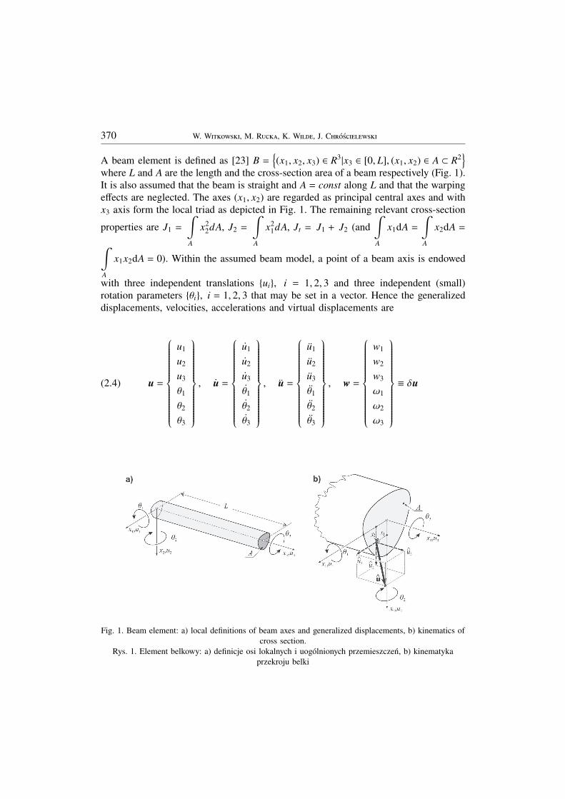
A beam element is defined as [23] B ={(x1, x2, x3) ∈ R3|x3 ∈ [0, L], (x1, x2) ∈ A ⊂ R2
}where L and A are the length and the cross-section area of a beam respectively (Fig. 1).It is also assumed that the beam is straight and A = const along L and that the warpingeffects are neglected. The axes (x1, x2) are regarded as principal central axes and withx3 axis form the local triad as depicted in Fig. 1. The remaining relevant cross-section
properties are J1 =
∫
A
x22dA, J2 =
∫
A
x21dA, Jt = J1 + J2 (and
∫
A
x1dA =
∫
A
x2dA =
∫
A
x1x2dA = 0). Within the assumed beam model, a point of a beam axis is endowed
with three independent translations {ui}, i = 1, 2, 3 and three independent (small)rotation parameters {θi}, i = 1, 2, 3 that may be set in a vector. Hence the generalizeddisplacements, velocities, accelerations and virtual displacements are
(2.4) u =
u1
u2
u3
θ1
θ2
θ3
, u =
u1
u2
u3
θ1
θ2
θ3
, u =
u1
u2
u3
θ1
θ2
θ3
, w =
w1
w2
w3
ω1
ω2
ω3
≡ δu
Fig. 1. Beam element: a) local definitions of beam axes and generalized displacements, b) kinematics ofcross section.
Rys. 1. Element belkowy: a) definicje osi lokalnych i uogólnionych przemieszczeń, b) kinematykaprzekroju belki

W . . . 371
For the sake of simplicity we use notation w ≡ δu though it should be noted that,in general, the test function w and variations δu play slightly different roles, which inour case in negligible.
Assuming the classical Timoshenko beam theory, an arbitrary (3D) point of cross--section area may undergo displacements given by
(2.5)
u(x1, x2, x3) =
u1
u2
u3
=
1 0 0 0 0 −x2
0 1 0 0 0 x1
0 0 1 x2 −x1 0
u1
u2
u3
θ1
θ2
θ3
= A(x1, x2) u(x3)
where A(x1, x2) is the matrix of constraints for 3D Timoshenko beam that enforceplane deformation of cross-section. The relevant strain-displacement equations thenfollow from usual definition of linear 3D strain (2) as
ε =
2ε31
2ε32
ε33
=
(.)′ 0 0 0 −1 −x2(.)′
0 (.)′ 0 1 0 x1(.)′
0 0 (.)′ x2(.)′ −x1(.)′ 0
u1
u2
u3
θ1
θ2
θ3
=(2.6)
u′1 − θ2 − x2θ′3
u′2 + θ1 + x1θ′3
u′3 + x2θ′1 − x1θ
′2
=
γ1 − x2κt
γ2 + x1κt
ε + x2κ1 − x1κ2
where (¤)′ = d(¤)/dx3. Using the definitions (6) the vector of beam strains ε withcomponents set in accordance with the order introduced in (4)1 may be written withthe help of matrix operator D

372 W. W, M. R, K. W, J. C
(2.7)
ε = Du, ε =
γ1
γ2
ε
κ1
κ2
κt
=
u′1 − θ2u′2 + θ1
u′3θ′1θ′2θ′3
=
(.)′ 0 0 0 −1 00 (.)′ 0 1 0 00 0 (.)′ 0 0 00 0 0 (.)′ 0 00 0 0 0 (.)′ 00 0 0 0 0 (.)′
u1
u2
u3
θ1
θ2
θ3
The generalized virtual strains of the beam are defined analogously
(2.8) δε = Dw, δε = { δγ1 δγ2 δε δκ1 δκ2 δκt }T
The resultant beam forces and couples (generalized stress) are respectively definedthrough specification constitutive equation of (3) for beam (see Appendix 1 for details)σ33 = Eε33, σ3α = 2Gε3α. Since we assume (x1, x2) are principal central axes then
(2.9)
W ≡∫
A
σ3dA⇒
T1 ≡∫
A
σ31dA =
∫
A
G(u′1 − θ2 − x2θ′3)dA = G
∫
A
γ31dA = GαsAγ31,
T2 ≡∫
A
σ32dA =
∫
A
G(u′2 + θ1 + x1θ′3)dA = G
∫
A
γ32dA = GαsAγ32,
N ≡∫
A
σ33dA =
∫
A
E(u′3 + x2θ′1 − x1θ
′2)dA = E
∫
A
dA
ε = EAε,
(2.10)
M≡∫
A
(r × σ3)dA⇒
M1 ≡∫
A
σ33 x2 dA =
∫
A
E(x2w′3 + x22θ′1 − x1x2θ
′2)dA = EJ1 κ1 ,
M2 ≡ −∫
A
σ33x1 dA = −∫
A
E(x1w′3 + x1x2θ′1−x2
1θ′2)dA = EJ2κ2, ,
Mt ≡∫
A
(σ32x1 − σ31x2)dA =
∫
A
G(x1γ2 + x21κt − x2γ1 + x2
2κt = )dA = GJtκt ,
where σ3(x1, x2, x3) = σ31e1 + σ32e2 + σ33e3 is three dimensional stress vector onelementary surface 3, r(x1, x2) = x1e1 + x2e2. The shear correction factor αs has been atopic of numerous analyses. Its physical sense on the grounds of mechanics of beams,plates and shells is well recognized. Typical values of αs are known and oscillate about

W . . . 373
1. For plates and shells they vary between to 1 (usually αs =56, cf. for instance [23])
depending on the assumed criterion, cf. for example [24, 25, 26, 27].By defining vector
(2.11) σ = { W T M T }T = { T1 T2 N M1 M2 Mt }T
equations (9) and (10) may be recast into following form
(2.12) σ = Eε, σ =
T1
T2
NM1
M2
Mt
=
GA1 0 0 0 0 00 GA2 0 0 0 00 0 EA 0 0 00 0 0 EJ1 0 00 0 0 0 EJ2 00 0 0 0 0 GJt
γ1
γ2
ε
κ1
κ2
κt
The positive sense of forces and moments is shown in Fig. 2a,b. Here qi and mi
are respectively functions of beam applied forces and couples per unit length, assumedto be energy conjugated with fields of translations and rotations. A vector of beamapplied forces and couples per unit length is defined as (cf. Fig. 2b)
(2.13) p = { q1 q2 qt m1 m2 mt }T
and the vector of forces and couples applied pointwise (and causing jumps of theinternal forces) applied at point (a) is (cf. Fig. 2c)
(2.14) P(a) = { P1a P2a P3a M1a M2a M3a }T
With definition of D from (7) the strong form of dynamic equilibrium equationsfor a beam segment in Fig. 2b may be stated in the following concise form
DTσ + p = ρJ u + µJ u,(2.15)
DT
(6×6)=
( .)′ 0 0 0 0 00 ( .)′ 0 0 0 00 0 ( .)′ 0 0 00 −1 0 ( .)′ 0 01 0 0 0 ( .)′ 00 0 0 0 0 ( .)′
, J(6×6)
=
A 0 0 0 0 00 A 0 0 0 00 0 A 0 0 00 0 0 J1 0 00 0 0 0 J2 00 0 0 0 0 Jt

374 W. W, M. R, K. W, J. C
Fig. 2. Definition of: a) forces, b) loads, c) jump of internal forces, d) finite segment of a beam for anintegral identity.
Rys. 2. Definicje: a) sił, b) obciążeń, c) skoków sił wewnętrznych, d) skończony element belki doformułowania tożsamości całkowej
Let us denote for further reference the jump conditions at point (a) (cf. Fig. 2c)
(2.16) P(a) − [[σ(a)]] = 0
where [[σ(a)]] = σL(a) − σP
(a) designates the jump of internal forces due to P(a) (ananalogous conditions may be written for other discontinuities/jumps e.g. frame nodes).
2.2. W
Consider a typical finite fragment of a beam l1−2 = x3(2) − x3(1) with beginning atx3(1) and end at x3(2), with one internal point of load discontinuity x3(a) (Fig. 2d). Letvector w(x3) (of the structure consistent with (4)4) designates arbitrary functions of x3,to which no physical meaning is assigned at the moment. By multiplying respectivelythe equilibrium conditions (15) and jump conditions (16) by w(x3), and w(x3(a)) thefollowing integral identity is obtained
(2.17)∫
l1−2\x3(a)
wT (DTσ + p − ρJu − µJu) dx3 + wT
(a)(P(a) − [[σ(a)]]) = 0
After some manipulations (17) reads

W . . . 375
−∫
l1−2\x3(a)
wT DTσdx3 + wT
(a)[[σ(a)]] +
∫
l1−2
wTρJudx3 +
∫
l1−2
wTµJudx3(2.18)
−∫
l1−2
wT pdx3 − wT(a)P(a) = 0
Integrating by parts i.e. (s2∫s1
F′u ds = −s2∫s1
Fu′ds + (Fu) |s2s1) the first term of (18)
becomes
(2.19) −∫
l1−2\ x3(a)
wT DTσdx3 =
∫
l1−2\ x3(a)
T(Dw)︸︷︷︸δε
σdx3 − wT(a)[[σ(a)]] − wT
(1)σ(1) + wT(2)σ(2)
In the above sense the operators DT and D are pseudo-conjugate.The integral identity (17) is valid for arbitrary segment l1−2, so it can be extended
on the whole structure taking into account all the point loads and other discontinu-ities. This operation requires taking into account both types of boundary conditions.Hence the field w is interpreted as the kinematically admissible virtual displacementw ≡ w. Therefore, apart from the continuity conditions required in the above mani-pulations, these functions must satisfy homogenous boundary conditions i.e. where-ver the boundary conditions are specified w vanish. As a result, the boundary terms−wT
(1)σ(1) + wT(2)σ(2) either disappear for specified displacements u∗(1) and u∗(2) or in-
crease the load vector (14) for given forces σ∗(1) and σ∗(2).Ultimately, considering the above in (18) the weak form of initial-boundary value
problem for a beam is
(2.20)∫
LwTρJudx3 +
∫
LwTηJudx3 +
∫
LδεTEε dx3 =
∫
LwT pdx3 +
∑awT
(a)P(a)
2.3. I,
Let Π(e) is a typical N-node finite element defined as a smooth image of the standardN-node element π(e) = [−1,+1] from the parent (natural) domain ξ ∈ π(e). All thevector variables of the problem are interpolated using the uniform and simultaneousLagrange interpolation. The Lagrange polynomials of order N − 1 satisfy the rules
(2.21) LNa (ξ) =
N∏
b=1, b,a
ξ − ξbξa − ξb , LN
a (ξb) = δab,∑N
a=1LN
a (ξ) = 1

376 W. W, M. R, K. W, J. C
where δab is the Kronceker delta. Hence at the a-th node (a = 1, 2, ...,N),
La(3×3)
(ξ) = LNa (ξ) 1
(3×3), La
(6×6)(ξ) =
La
(3×3)(ξ) 0
(3×3)
0(3×3)
La(3×3)
(ξ)
,(2.22)
1(3×3)
=
1 0 00 1 00 0 1
, 0(3×3)
=
0 0 00 0 00 0 0
while for the whole N-th node element
(2.23) L(e)(ξ) = [L1(ξ)|L2(ξ)|...|LN (ξ)], L(e)(ξ) = [L1(ξ)|L2(ξ)|...|LN (ξ)]
By defining respectively for a−th node (a = 1, 2, ...,N):position vector
(2.24) x→ xa =
x1
x2
x3
a
=
x1a
x2a
x3a
nodal vector rmua of generalized displacements and nodal vector wa of variations ofgeneralized displacements
(2.25) u→ ua =
u1
u2
u3
θ1
θ2
θ3
a
=
u1a
u2a
u3a
θ1a
θ2a
θ3a
, w→ wa =
w1
w2
w3
ω1
ω2
ω3
a
=
w1a
w2a
w3a
ω1a
ω2a
ω3a
,
nodal vector ua of velocities of generalized displacements and nodal vector ua ofaccelerations of generalized displacements

W . . . 377
(2.26) u→ ua =
u1
u2
u3
θ1
θ2
θ3
a
=
u1a
u2a
u3a
v1a
θ2a
θ3a
, u→ ua =
u1
u2
u3
θ1
θ2
θ3
a
=
u1a
u2a
u3a
θ1a
θ2a
θ3a
within an element the following interpolation schemes hold
(2.27) x(ξ) = L(e)(ξ)x(e), x(e) = {x1, x2, ..., xN }T ,
(2.28) u(ξ, t) = L(e)(ξ) u(e)(t), u(e)(t) = {u1(t), u2(t), ..., uN (t)}T ,
(2.29) w(ξ) = L(e)(ξ) w(e), w(e) = {w1,w2, ...,wN }T ,
(2.30) u(ξ, t) = L(e)(ξ) u(e)(t), u(e)(t) = {u1(t), u2(t), ..., uN (t)}T
(2.31) u(ξ, t) = L(e)(ξ) u(e)(t), u(e)(t) = {u1(t), u2(t), ..., uN (t)}T
(2.32) ε(ξ, t) = DL(e)(ξ) u(e)(t) = B(e)(ξ) u(e)(t), δε(ξ) = DL(e)(ξ)w(e) = B(e)(ξ)w(e)
where strain-displacement operator of an element is
(2.33) B(e)(ξ) = [B1(ξ)|B2(ξ)|...|BN (ξ)]
Here nodal matrix Ba(ξ)(6×6)
follows from (7) and (22), and is defined as

378 W. W, M. R, K. W, J. C
(2.34)
Ba(6×6)
(ξ) = DL(a)(ξ) =
(LNa (ξ))′ 0 0
∣∣∣∣ 0 −LNa (ξ) 0
0 (LNa (ξ))′ 0
∣∣∣∣ LNa (ξ) 0 0
0 0 (LNa (ξ))′
∣∣∣∣ 0 0 0
0 0 0∣∣∣∣ (LN
a (ξ))′ 0 0
0 0 0∣∣∣∣ 0 (LN
a (ξ))′ 0
0 0 0∣∣∣∣ 0 0 (LN
a (ξ))′
Substitution of interpolation schemes into (20) yields the following definitions ofelement stiffness matrix, mass matrix, damping matrix, and load vector
∫
L
δεTEεdx3 =
∫
L
(Dw)TEDudx3interpolation→
∫
L
(DL(e)(ξ)w(e))TEDL(e)(ξ)u(e)dx3
= wT(e)K(e)u(e) → K(e) =
∫
L
BT(e)(ξ) EB(e)(ξ) dx3
,
(2.35)
(2.36)
∫
L
wTρJudx3interpolation→
∫
L
(L(e)(ξ)w(e))TρJL(e)(ξ)u(e)dx3
= wT(e)M(e)u(e) → M(e) = ρ
∫
L
LT(e)(ξ) JL(e)(ξ) dx3
,
(2.37)
c∫
L
wT Judx3interpolation→ c
∫
L
(L(e)(ξ)w(e))T JL(e)(ξ)u(e)dx3
= wT(e)C(e)u(e) → C(e) = c
∫
L
LT(e)(ξ) JL(e)(ξ) dx3
,
(2.38)
∫
L
wT pdx3 +∑
awT
(a)P(a)interpolation→
∫
L
(L(e)(ξ) w(e))T pdx3 +∑
a
wT(a)P(a)
= wT(e)
∫
L
LT(e)(ξ) pdx3
+ wT(e)P(e)
= wT(e)f(e) → f(e) = f ext
(e) + f nod(e)
,

W . . . 379
where f ext(e) =
∫
L
LT(e)(ξ) pdx3, f nod
(e) = {P1 P2 ...PN }T . Since w(e) are arbitrary, the matrix
form of (20) in local frame of an element reads
(2.39) M(e)u(e) + C(e)u(e) + K(e)u(e) = f(e)
For future reference we define element vectors of: inertia, damping and internalforces respectively
(2.40) b(e) = M(e)u(e), c(e) = C(e)u(e), r(e) = K(e)u(e)
Furthermore, the Jacobian determinant j = det(∂x/∂ξ) (cf. [23]) necessary inisoparametric formulation reads
(2.41) j(ξ) = det(∂x/∂ξ) =∑N
a=1
dL(aξ)
dξxa
where La(ξ) is defined in (22)1. Thus the relation for element length becomes dx3 =
j(ξ)dξ. The element matrices computed numerically according employing Lobattoquadrature rule. The methodology is the same as that discussed in [22] and hence isnot repeated here. Note only, that the mass matrix and damping matrix of an elementwill be diagonal provided that integration points of quadrature rule coincide withelement’s nodes of Lagrange interpolation polynomials in natural coordinate, whichfollows from (21).
As a consequence the mass matrix and damping matrix become respectively
(2.42)
M(e) →[M(e)
ii
]→ ρ
J(6×6)
w1 j(ξ1) 0(6×6)
· · · 0(6×6)
0(6×6)
J(6×6)
w2 j(ξ2) · · · 0(6×6)
......
. . ....
0(6×6)
0(6×6)
· · · J(6×6)
wN j(ξN )
(6N×6N)
, M(e)i j = 0, i , j
(2.43) C(e) = ηM(e)
where N ∈ [1,M] is the number of integration point ξN . The integration points areplaced irregularly in coordinate system which removes the undesired Runge effect.

380 W. W, M. R, K. W, J. C
2.4. T
Following [26] the end nodes are referred to structural coordinate system while internalnodes remain in local frame. As a consequence, in the considered N–node beamelement the structural displacement q(e) vector takes the form
(2.44)q(e) = [qT
1 , uT2 , ..., u
TN−1, q
TN ]T , qa =
{u1a u2a u3a θ1a θ2a θ3a
}T, a = 1,N
with uA, A ∈ [2,N − 1] given by (25). The transformation matrix T(e) that enablesrotation of the local axes to the structural axes reads
(2.45)
u(e) = T(e)q(e), T(e)N×N
=
QT
(6×6)0
(6×6(N−2))0
(6×6)
0(6(N−2)×6)
1(6(N−2)×6(N−2))
0(6(N−2)×6)
0(6×6)
0(6×6(N−2))
QT
(6×6)
, 1
(6(N−2)×6(N−2))=
I(6×6)
· · · 0(6×6)
.... . .
...
0(6×6)
· · · I(6×6)
In (45) the matrices are defined as follows.
(2.46) I(6×6)
=
1
(3×3)0
(3×3)
0(3×3)
1(3×3)
, 0(6×6)
=
0
(3×3)0
(3×3)
0(3×3)
0(3×3)
, Q(6×6)
=
Q
(3×3)0
(3×3)
0(3×3)
Q(3×3)
where 1(3×3)
and 0(3×3)
are defined in (23) and
(2.47) Q(3×3)
= [t1 t2 t3], t1 =
cosα11
cosα12
cosα13
, t2 =
cosα21
cosα22
cosα23
, t3 =
cosα31
cosα32
cosα33
The transformation of local element stiffness matrix K(e) and element load vectorf(e) to structural coordinate system is K(e) = TT
(e)K(e)T(e), f(e) = TT(e)f(e), r(e) = TT
(e)r(e).The element mass matrix and element damping matrix are respectively transformed asthe stiffness matrix, whereas the element vectors (40) undergo the following transfor-mations b(e) = TT
(e)b(e), c(e) = TT(e)c(e), r(e) = TT
(e)r(e). It should be noted that the notationsdescribing the transformation are only formal. In own Fortran code we exploit thestructure of transformation matrix T(e) and the time consuming matrix multiplicationsby 1(6(N−2)×6(N−2)) are not performed.
The final (semi-discrete) system of equation of motion and equilibrium conditionare populated using standard aggregation procedure and are written as

W . . . 381
(2.48) Mq + Cq + Kq = p, j = p − b(q) − c(q) − r(q) = 0
where q, q and q are structural vectors of displacements, accelerations and velocities,respectively. Equation (48) is approximated in time domain following precisely thesame scheme as elaborated in [22]. For the sake of completeness let us recall the mostimportant aspects of the employed time integration scheme.
2.5. T
The algorithm uses accelerations as the primary variables and takes the advantageof the structure of mass and damping matrices. Let tn+1 = tn + ∆t denote the timediscretization. and assume that all required values up to step n are already known.Writing now (48)1 as
(2.49) Mqn+1 + Cqn+1 = pn+1 − r(qn+1)
where r(qn+1) is found from aggregation r = ANeleme=1 r(e) removes the explicit presence of
global stiffness matrix K which is of full structure. Due to the presence of qn+1 on theright hand side of (49) the scheme requires iteration. Substitution of iterative notationi.e.,
(2.50) q(i+1)n+1 = q(i)
n+1 + δq
(2.51) q(i+1)n+1 = qn + ∆t [(1 − γ)qn + γq(i)
n+1] + ∆tγδq
(2.52) q(i+1)n+1 = qn + ∆tqn + 1
2 (∆t)2[(1 − 2β)qn + 2βq(i)n+1] + (∆t)2βδq
into (49) yields implicit equation with respect to iteration correction δq
(2.53)[M + ∆tγC
]δq = pn+1 − b(i)
n+1 − c(i)n+1 − r(q(i)
n+1 + (∆t)2βδq)
Equation (53) is solved for δq using simple iteration method i.e.
(2.54) δq =[M + ∆tγC
]−1 (pn+1 − b(i)
n+1 − c(i)n+1 − r(q(i)
n+1))
382 W. W, M. R, K. W, J. C
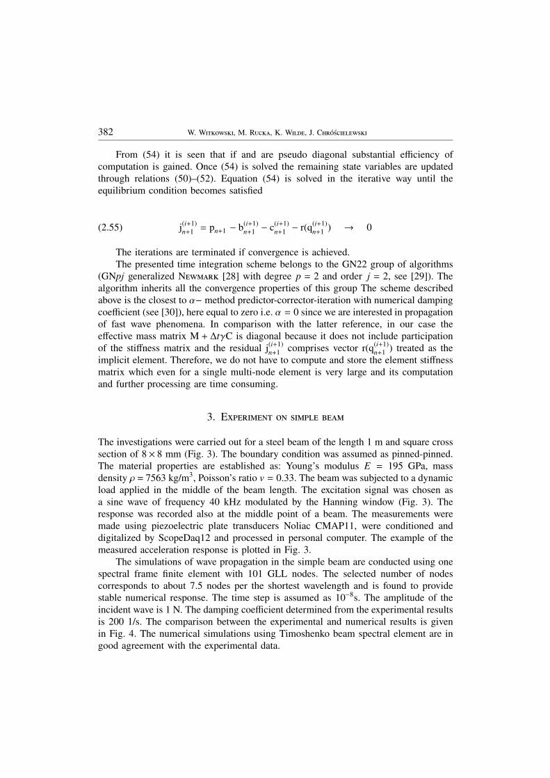
From (54) it is seen that if and are pseudo diagonal substantial efficiency ofcomputation is gained. Once (54) is solved the remaining state variables are updatedthrough relations (50)–(52). Equation (54) is solved in the iterative way until theequilibrium condition becomes satisfied
(2.55) j(i+1)n+1 = pn+1 − b(i+1)
n+1 − c(i+1)n+1 − r(q(i+1)
n+1 ) → 0
The iterations are terminated if convergence is achieved.The presented time integration scheme belongs to the GN22 group of algorithms
(GNpj generalized N [28] with degree p = 2 and order j = 2, see [29]). Thealgorithm inherits all the convergence properties of this group The scheme describedabove is the closest to α− method predictor-corrector-iteration with numerical dampingcoefficient (see [30]), here equal to zero i.e. α = 0 since we are interested in propagationof fast wave phenomena. In comparison with the latter reference, in our case theeffective mass matrix M + ∆tγC is diagonal because it does not include participationof the stiffness matrix and the residual j(i+1)
n+1 comprises vector r(q(i+1)n+1 ) treated as the
implicit element. Therefore, we do not have to compute and store the element stiffnessmatrix which even for a single multi-node element is very large and its computationand further processing are time consuming.
3. E
The investigations were carried out for a steel beam of the length 1 m and square crosssection of 8 × 8 mm (Fig. 3). The boundary condition was assumed as pinned-pinned.The material properties are established as: Young’s modulus E = 195 GPa, massdensity ρ = 7563 kg/m3, Poisson’s ratio v = 0.33. The beam was subjected to a dynamicload applied in the middle of the beam length. The excitation signal was chosen asa sine wave of frequency 40 kHz modulated by the Hanning window (Fig. 3). Theresponse was recorded also at the middle point of a beam. The measurements weremade using piezoelectric plate transducers Noliac CMAP11, were conditioned anddigitalized by ScopeDaq12 and processed in personal computer. The example of themeasured acceleration response is plotted in Fig. 3.
The simulations of wave propagation in the simple beam are conducted using onespectral frame finite element with 101 GLL nodes. The selected number of nodescorresponds to about 7.5 nodes per the shortest wavelength and is found to providestable numerical response. The time step is assumed as 10−8s. The amplitude of theincident wave is 1 N. The damping coefficient determined from the experimental resultsis 200 1/s. The comparison between the experimental and numerical results is givenin Fig. 4. The numerical simulations using Timoshenko beam spectral element are ingood agreement with the experimental data.

W . . . 383
Fig. 3. Steel beam: a) geometry; b) load; c) experimental signal.Rys. 3. Belka stalowa: a) geometria, b) obciążenie, c) sygnał z eksperymentu
Fig. 4. Wave propagation in steel beam: a) numerical signal; b) comparison of experimental andnumerical signals.
Rys. 4. Propagacja fal w belce stalowej: a) wynik numeryczny, b) porównanie eksperymentu z wynikaminumerycznymi
4. N
4.1. S
The first example is a simple three dimensional frame analyzed for possible applicationof elastic waves for structural health monitoring. The frame has three equal arms(Fig. 5) of length 1m. The frame elements have square cross section of dimension8 × 8 mm. The frame is made of steel with modulus of elasticity E = 210 GPa, massdensity ρ = 7850 kg/m3 and Poisson ratio v = 0.33. The moments of inertia are:J1 = J2 = 3.41(3) · 10−10 m4, Jt = 5.7344 · 10−10 m4. The damage is modelled byintroduced additional masses and the time responses of the waves propagating in thestructure with and without damage are compared.
384 W. W, M. R, K. W, J. C
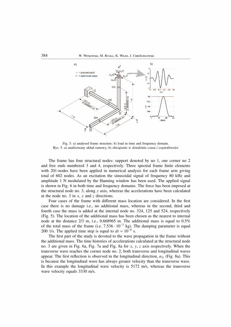
Fig. 5. a) analysed frame structure; b) load in time and frequency domain.Rys. 5. a) analizowany układ ramowy, b) obciążenie w dziedzinie czasu i częstotliwości
The frame has four structural nodes: support denoted by no 1, one corner no 2and free ends numbered 3 and 4, respectively. Three spectral frame finite elementswith 201-nodes have been applied in numerical analysis for each frame arm givingtotal of 602 nodes. As an excitation the sinusoidal signal of frequency 80 kHz andamplitude 1 N modulated by the Hanning window has been used. The applied signalis shown in Fig. 6 in both time and frequency domains. The force has been imposed atthe structural node no. 3, along y axis, whereas the accelerations have been calculatedat the node no. 3 in x, y and z directions.
Four cases of the frame with different mass location are considered. In the firstcase there is no damage i.e., no additional mass, whereas in the second, third andfourth case the mass is added at the internal node no. 324, 125 and 524, respectively(Fig. 5). The location of the additional mass has been chosen as the nearest to internalnode at the distance 2/3 m, i.e., 0.668965 m. The additional mass is equal to 0.5%of the total mass of the frame (i.e. 7.536 · 10−3 kg). The damping parameter is equal200 1/s. The applied time step is equal to dt = 10−8 s.
The first part of the study is devoted to the wave propagation in the frame withoutthe additional mass. The time histories of accelerations calculated at the structural nodeno. 3 are given in Fig. 6a, Fig. 7a and Fig. 8a for x, y, z axis respectively. When thetransverse wave reaches the corner node no. 2, both transverse and longitudinal wavesappear. The first reflection is observed in the longitudinal direction, a3z (Fig. 8a). Thisis because the longitudinal wave has always greater velocity than the transverse wave.In this example the longitudinal wave velocity is 5172 m/s, whereas the transversewave velocity equals 3330 m/s.

W . . . 385
Fig. 6. Acceleration time histories in node no. 3 (x direction): a) ideal frame; b) frame with mass atnode no. 126; c) frame with mass at node no. 325; d) frame with mass at node no. 524.
Rys. 6. Przebiegi czasowe przyspieszenia w kierunku x w węźle 3: a) konstrukcja idealna, b) konstrukcjaz masą w węźle 126, c) konstrukcja z masą w węźle 325, d) konstrukcja z masą w węźle 524
The results for the frame with the additional mass placed at the internal node no.325 are given in Fig. 6c, Fig. 7c and Fig. 8c for the x, y and z directions, respectively.There are visible peaks corresponding to the wave reflections from the frame structuralnodes (the same as with the frame without the additional mass) as well as from theadditional mass. The mass position can be easily identified because the excitation,response and mass are within the same element. The time of the reflection from theadditional mass is found to be 0.2 ms. Analysis of the reflection time and the wavespeed enables the estimate the placement of the additional mass as 0.33 m from theelement free end.
In the next examples the additional mass has been placed at the internal nodeno. 126 (Fig. 6b, Fig. 7b and Fig. 8b). In this case, the mass is on the different elementthan the excitation and response measurement point, therefore, the transition of thewave through the structural node is required. This situation is important in the context

386 W. W, M. R, K. W, J. C
Fig. 7. Acceleration time histories in node no. 3 (ydirection): a) ideal frame; b) frame with mass at nodeno. 126; c) frame with mass at node no. 325; d) frame with mass at node no. 524.
Rys. 7. Przebiegi czasowe przyspieszenia w kierunku y w węźle 3: a) konstrukcja idealna, b) konstrukcjaz masą w węźle 126, c) konstrukcja z masą w węźle 325, d) konstrukcja z masą w węźle 524
of application of this method to structural health monitoring. The mass position canbe identified as 0.33 m from node no. 2.
The last example concerns the additional mass located in the internal node no. 524(Fig. 6d, Fig. 7d and Fig. 8d). In this case only the acceleration along x axis indicatesthe additional reflection that can be used for calculation of damage position. In thiscase the location of the mass is also correct.
The snapshots from the animations for the ideal frame are given in Fig 9. Inthe first time instance 0.1 ms only transverse waves propagates from node 3 towardsnode 2. In the second time instance 0.4 ms, the incident wave reaches the node 2 andcauses propagation of all types of waves, i.e., longitudinal and transverse with respectto local x1 and x3 axis, in all frame elements. At the time 0.5 ms, the longitudinal wavereaches the node no. 3, whereas the transverse wave propagates through the vertical

W . . . 387
Fig. 8. Acceleration time histories in node no. 3 (z direction): a) ideal frame; b) frame with mass atnode no. 126; c) frame with mass at node no. 325; d) frame with mass at node no. 524.
Rys. 8. Przebiegi czasowe przyspieszenia w kierunku z w węźle 3: a) konstrukcja idealna, b) konstrukcjaz masą w węźle 126, c) konstrukcja z masą w węźle 325, d) konstrukcja z masą w węźle 524
element of the frame. Fig. 10 presents the snapshot for the frame with the additionalmass at the node no. 126. The additional reflections from the lumped mass are clearlyvisible.
4.2. S
The second example verifies the possibility of tracing the elastic waves in more com-plicated 3D frame structure. The considered frame structure, shown in Fig. 11, isnamed star dome and is taken after, e.g. [31]. The structure possesses six symmetryaxes which is useful in the validation of the numerical results. The material proper-ties are: modulus of elasticity E = 210 GPa, Poisson’s ratio v = 0.33, mass density

388 W. W, M. R, K. W, J. C
Fig. 9. Animation of wave propagation in ideal frame at the selected time instances: a) t = 0.1 ms;b) t = 0.4 ms; c) t = 0.5 ms; d) t = 0.8 ms.
Rys. 9. Animacja propagacji fali w ramie idealnej w wybranych chwilach czasowych: a) t = 0,1 ms;b) t = 0,4 ms; c) t = 0,5 ms; d) t = 0,8 ms

W . . . 389
Fig. 10. Animation of wave propagation in frame with additional mass at the selected time instances:a) t = 0.1 ms; b) t = 0.4 ms; c) t = 0.5 ms; d) t = 0.8 ms.
Rys. 10. Animacja propagacji fali w ramie z dodatkową masą w wybranych chwilach czasowych:a) t = 0,1 ms; b) t = 0,4 ms; c) t = 0,5 ms; d) t = 0,8 ms

390 W. W, M. R, K. W, J. C
ρ = 7850 kg/m3, damping coefficient η = ρ/c = 200 1/s. The moments of inertia are:J1 = 4.16(7) · 10−11 m4, J2 = 2.66(7) · 10−11 m4, Jt = 5.376 · 10−11 m4 and the elementarea is A = 2 · 10−7 m2. To simplify the modelling, the local axis x2 of each elementis pointed vertically towards the origin of the global coordinate system.
Fig. 11. The star dome: a) geometry; b) load in time and frequency domain.Rys. 11. Przestrzenna rama w kształcie kopuły: a) geometria, b) obciążenie w dziedzinie
czasu i częstotliwości
As an excitation a sinusoidal signal of amplitude 1 N and frequency 200 kHzmodulated by the Hanning window has been applied (Fig. 11). The load has beenplaced at the node 13 of the structure model along the global z axis. The total timeof load action is t = 0.02 ms. The number of nodes per one spectral element is set to161, which gives about 10 nodes per the shortest considered wavelength in the shorteststar dome element. The integration time step is dt = 5 · 10−9s.
The elastic wave propagation computed by the Timoshenko beam spectral model iscompared with the results computed by a truss model, [22], for the same structure. Inthe case of truss element, the transverse wave does not appear, therefore, the wavelengthis longer. However, in truss element also 161 nodes are used for comparison purpose.The time step has been assumed as dt = 10−8s.
The snapshots of the wave propagation in the case 1, loading at the node no.13 along global z axis, are given in Fig. 12. The graphs have been obtained usingGiD software [32]. The results show the longitudinal waves travelling along the local

W . . . 391
elements axis. The first time instance in Fig. 12. has been selected as 0.01 ms, whenthe front of the wave starts to propagate. In the case of the frame model (Fig. 12a)the impact of the external force induces propagation of waves in all six elements inthe neighbourhood of the node 13 forwards the bottom of the dome (t = 0.025 ms). Inthe time instance t = 0.05 ms the waves reach the nodes no. 2, 4, 6, 8, 10 and 12 andthe reflections take place. The amplitudes of the waves that are coming back to thetop are slightly larger form the amplitudes of the waves going down to the supports(t = 0.075 ms).
Fig. 12. Animation of longitudinal wave propagation caused by impacting of node no. 13 at the timeinstances: a) frame model; b) truss model.
Rys. 12. Animacja propagacji fali wzdłużnej wywołanej uderzeniem w węzeł 13 w chwilach czasowych:a) model ramowy, b) model kratowy
In Fig. 13, Fig. 14, Fig. 15, Fig. 16 and Fig. 17 the route of wave from the top (node13) to the support (node 14) is traced. The acceleration time history at the beginningof the element is presented on the example of node 649 (Fig. 13) that is located very

392 W. W, M. R, K. W, J. C
close to the central node 13. The results are plotted with respect to the element localaxis. Due to the structure symmetry the accelerations along x1 are equal zero in allthe roof elements passing through node 13 (Fig. 13a). The acceleration along x2 axishas five visible wave forms within the considered time up to 0.3 ms (Fig. 13b). Thefirst wave is the initial wave resulting from the external excitation loaded at the domecentral point. The fourth wave present at time t = 0.158 has relatively large amplitudeand is induced by the reflection of the transverse wave from the node no. 2, i.e., thearrival time is the time necessary to travel from node 13 to node 2 multiplied by two.
Fig. 13. Acceleration time histories for frame model (impact: node no 13, response: node no. 649).Rys. 13. Przebiegi czasowe przyspieszenia w modelu ramowym (uderzenie w węźle 13, odpowiedź
w węźle 649)
The fifth wave form appearing at time t = 0.237 ms is a summation of transversewaves travelling between the nodes 13, 4, 2, 13 and nodes 13, 12, 2, 13. The travellingtime is equal to the time necessary to travel through the single element multiplied bythree. Waveforms denoted by no. 1, 4, and 5 are transverse waves and are dominantin the acceleration response at node 649. The second and third wave forms arrive attime t = 0.096 ms and t = 0.127 ms, respectively. The second wave comes from thelongitudinal wave that reflects from node number 2 and comes back to node 13. Thethird wave form is a summation of the wave that travels as transverse wave to node 2and comes back as a longitudinal reflection from node 2, as well as the longitudinalwave that comes back as transverse which component is visible in node 649, afterreflection from node 13. The amplitudes of wave forms no. 3 and 4 are considerablysmaller than amplitudes of waves resulting from the initial transverse wave (waveformsdenoted by 1, 4, and 5).

W . . . 393
Fig. 14. Acceleration time histories for frame model (impact: node no 13, response: node no. 570).Rys. 14. Przebiegi czasowe przyspieszenia w modelu ramowym (uderzenie w węźle 13, odpowiedź
w węźle 570)
Fig. 15. Acceleration time histories for frame model (impact: node no 13, response: node no. 491).Rys. 15. Przebiegi czasowe przyspieszenia w modelu ramowym (uderzenie w węźle 13, odpowiedź
w węźle 491)

394 W. W, M. R, K. W, J. C
Fig. 16. Acceleration time histories for frame model (impact: node no 13, response: node no. 172).Rys. 16. Przebiegi czasowe przyspieszenia w modelu ramowym (uderzenie w węźle 13, odpowiedź
w węźle 172)
Fig. 17. Acceleration time histories for frame model (impact: node no 13, response: node no. 14).Rys. 17. Przebiegi czasowe przyspieszenia w modelu ramowym (uderzenie w węźle 13, odpowiedź
w węźle 14)
W . . . 395
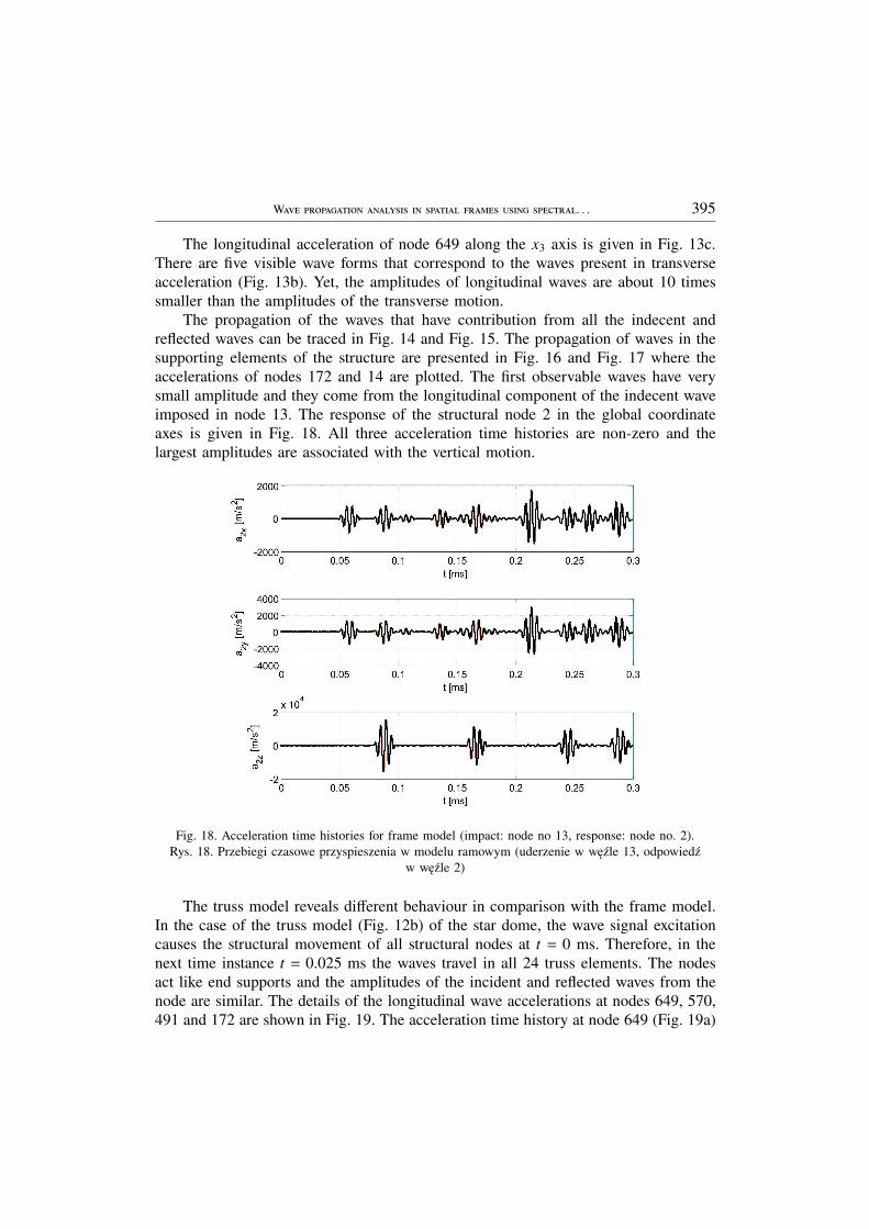
The longitudinal acceleration of node 649 along the x3 axis is given in Fig. 13c.There are five visible wave forms that correspond to the waves present in transverseacceleration (Fig. 13b). Yet, the amplitudes of longitudinal waves are about 10 timessmaller than the amplitudes of the transverse motion.
The propagation of the waves that have contribution from all the indecent andreflected waves can be traced in Fig. 14 and Fig. 15. The propagation of waves in thesupporting elements of the structure are presented in Fig. 16 and Fig. 17 where theaccelerations of nodes 172 and 14 are plotted. The first observable waves have verysmall amplitude and they come from the longitudinal component of the indecent waveimposed in node 13. The response of the structural node 2 in the global coordinateaxes is given in Fig. 18. All three acceleration time histories are non-zero and thelargest amplitudes are associated with the vertical motion.
Fig. 18. Acceleration time histories for frame model (impact: node no 13, response: node no. 2).Rys. 18. Przebiegi czasowe przyspieszenia w modelu ramowym (uderzenie w węźle 13, odpowiedź
w węźle 2)
The truss model reveals different behaviour in comparison with the frame model.In the case of the truss model (Fig. 12b) of the star dome, the wave signal excitationcauses the structural movement of all structural nodes at t = 0 ms. Therefore, in thenext time instance t = 0.025 ms the waves travel in all 24 truss elements. The nodesact like end supports and the amplitudes of the incident and reflected waves from thenode are similar. The details of the longitudinal wave accelerations at nodes 649, 570,491 and 172 are shown in Fig. 19. The acceleration time history at node 649 (Fig. 19a)

396 W. W, M. R, K. W, J. C
shows the indecent wave at time t = 0 s and the wave reflected form the node 2 at timet = 0.096 ms depicted by dotted line. Since the node is located very near the structuralnode 13, the second wave form has very small amplitude. It is because the reflectedwave is 180 degree phase shifted with respect to the incoming wave, and thus, a sumof both waves results in wave form of amplitude about 2 m/s2. The second, third,fourth and fifth waves at acceleration records at nodes 491 and 171 have very smallamplitudes due to the same reason. The waves not affected by the boundary conditionof the single element can be seen in Fig. 19b, where the acceleration record at themiddle of the element is presented.
Fig. 19. Acceleration time histories for truss model: a) node no. 649; b) node no. 570; c) node no. 491;d) node no. 172.
Rys. 19. Przebiegi czasowe przyspieszenia w modelu kratowym: a) węzeł nr 649, b) węzeł nr 570,c) węzeł nr 491, d) węzeł nr 172
W . . . 397
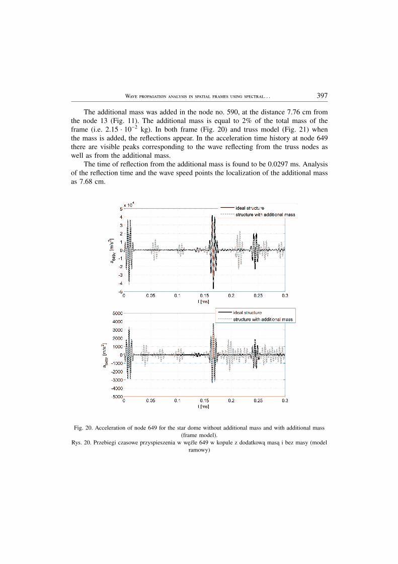
The additional mass was added in the node no. 590, at the distance 7.76 cm fromthe node 13 (Fig. 11). The additional mass is equal to 2% of the total mass of theframe (i.e. 2.15 · 10−2 kg). In both frame (Fig. 20) and truss model (Fig. 21) whenthe mass is added, the reflections appear. In the acceleration time history at node 649there are visible peaks corresponding to the wave reflecting from the truss nodes aswell as from the additional mass.
The time of reflection from the additional mass is found to be 0.0297 ms. Analysisof the reflection time and the wave speed points the localization of the additional massas 7.68 cm.
Fig. 20. Acceleration of node 649 for the star dome without additional mass and with additional mass(frame model).
Rys. 20. Przebiegi czasowe przyspieszenia w węźle 649 w kopule z dodatkową masą i bez masy (modelramowy)

398 W. W, M. R, K. W, J. C
Fig. 21. Acceleration of node 649 for the star dome without additional mass and with additional mass(truss model).
Rys. 21. Przebiegi czasowe przyspieszenia w węźle 649 w kopule z dodatkową masą i bez masy (modelkratowy)
5. C
In this paper the spectral element method model for spatial frames is presented. Thenumerical simulations are conducted on the two examples of the structures. The mo-delling of the frames was performed by the spectral element method with the GLLintegration rule. The wave propagation time histories for the structure with and witho-ut the additional mass are analyzed. The time of wave reflections arrival is used forthe calculation of the additional mass location. The results of the wave propagation,calculated by the frame model are compared with the results obtained using trussmodel.
The study on modelling of wave propagation in the spatial frames structures leadsto the following conclusions and suggestions:

W . . . 399
a) It is possible to detect singularity from the numerical results, even if the singula-rity is situated within different element than the location of the loading or accelerationmeasurement. For the frame with few elements, the SHM can be equipped with only onetransducers. However, in a more complicated structure the wave propagation patternsbecome very complicated and large number of the transducers should be used.
b) The frame model seems to be more appropriate for numerical simulation ofelastic wave propagation phenomena in spatial trusses than truss model.
c) The numerical results have to be compared with the experimental study whichinclude the structural nodes so the reflection of the incoming wave is captured.
6. A
The authors are grateful to the support of the Polish Ministry of Science and HigherEducation via Grant no. N506 065 31/3149 entitled: “Multilevel damage detectionsystem in engineering structures”.
A 1
The constitutive equation (3) in components yields
(56) σi j = λεkkδi j + 2Gεi j
Under assumption that σαβ = 0, (56) becomes
(57) σαβ = 0 = λεkkδαβ + 2Gεαβ
Subjected to contraction the latter equation yields
(58) 0 = λεkkδαα + 2Gεαα ⇒ εαα =−λε33
λ + µ
Thus from (56)
(59) σ33 = λεkk + 2Gε33 = λ (εαα + ε33) + 2Gε33 = λεαα + (2G + λ) ε33
and after some manipulations
(60) σ33 = Eε33

400 W. W, M. R, K. W, J. C
The remaining necessary components of stress tensor are
(61) σα3 = λεkkδα3 + 2Gεα3 = 2Gεα3, α, β = 1, 2
R
1. C. R. F , S. W. D, Damage detection II: Field Applications to Large Structures, in ModalAnalysis and Testing. Dordrecht, Netherlands: J. M. M. Silva and N. M. M. Maia, edts., Nato ScienceSeries, Kluwer Academic Publishers, 1999.
2. P. C, R. D. A, The location of defects in structures from measurements natural frequencies,Journal of Strain Analysis 14, 49-57, 1979.
3. J-T. K, Y-S. R, H-M. C, N. S, Damage identification in beam-type structures: frequencybased method vs mode-shape-based method, Engineering Structures 25, 57-67, 2003.
4. A. M, Detecting damage in beams through digital differentiator filters and continuous wavelettransforms, Journal of Sound and Vibration 272, 385-412, 2004.
5. S. K, Z. Z, Damage reconstruction of 3d frames using genetic algorithms with Levenberg--Marquardt local search, Soil Dynamics & Earthquake Engineering 29, 311-323, 2008.
6. M. R, K. W, Application of continuous wavelet transform in vibration based damage detectionmethod for beam and plates, Journal of Sound and Vibration 297, 536-550, 2006.
7. M. J. S. L, D. N. A, P. C, Defect detection in pipes using guided waves, Ultrasonics36, 147-154, 1998.
8. R. P. D, P. C, M. J. S. L, The potential of guided waves for monitoring large areas ofmetallic aircraft fuselage structures, Journal of Nondestructive Evaluation 20, 29-46, 2001.
9. J. F. D, Wave propagation in structures: spectral analysis using fast discrete Fourier transforms(second ed.), Springer-Verlag, New York 1997.
10. M. K, M. P, W. O, The dynamic analysis of a cracked Timoshenko beam bythe spectral element method, Journal of Sound and Vibration 264, 1139-1153, 2003.
11. S. G, A. C, D. R-M, Spectral finite element method: wave propa-gation, diagnostics and control in anisotropic and inhomogeneous structures, Springer-Verlag, London2008.
12. A. C, S. G, A spectrally formulated plate element for wave propagationanalysis in anisotropic material, Computer Methods in Applied Mechanics and Engineering 194,4425-4446, 2005.
13. A. C, S. G, A spectrally formulated finite element for wave propagationanalysis in layered composite media, International Journal of Solids and Structures 41, 5155-5183,2004.
14. D. S. K, D. R-M, S. G, A spectral finite element for wave propaga-tion and structural diagnostic analysis of composite beam with transverse crack, Finite Elements inAnalysis and Design 40, 1729-1751, 2004.
15. R. D. M, S. G, Spectral finite analysis of coupled wave propagation in com-posite beams with multiple delaminations and strip inclusions, International Journal of Solids andStructures 41, 1173-1208, 2004.
16. R. D. M, S. G, A spectral finite element for analysis of wave propagation inuniform composite tubes, Journal of Sound and Vibration 268, 429-463, 2003.

W . . . 401
17. H. I, K. K, I. Y, T. K, Wave propagation analysis of frame structures usingthe spectral element method, Journal of Sound and Vibration 227, 1071-1081, 2004.
18. T. P, A spectral element method for fluid dynamics: laminar flow in a channel expansion, Journalof Computational Physics 54, 468-488, 1984.
19. C. C, M.Y. H, A. Q, T.A. Z, Spectral methods in fluid dynamics, SpringerVerlag, Berlin, Heidelberg 1998.
20. R. S, A. C, S. G, Wave propagation analysis in anisotropic and inho-mogeneous uncracked and cracked structures using pseudospectral finite element method, InternationalJournal of Solids and Structures 43, 4997-5031, 2006.
21. P. K, M. K, W. O, Wave propagation modelling in 1D structures usingspectral finite elements, Journal of Sound and Vibration 300, 88-100, 2007.
22. J. C, M. R, K. W, W. W, Formulation of spectral truss element forguided waves damage detection in spatial steel trusses, Archives of Civil Engineering 55, 43-63,2009.
23. T. J. R. H, The Finite Element Method: linear static and dynamics finite element analysis, DoverPublications, Inc., Mineola, New York 2000.
24. J. C, J. M, W. P, Statyka i dynamika powłok wielopłatowych,IPPT PAN, Warszawa 2004.
25. Z. R, On the shear coefficient in beam bending, Mech. Res. Comm., 14, 379-385, 1987.26. S. J, The effects of constrained cross-sectional warping on the bending of beames, J. Theor.
Appl. Mech., 36, 121-144, 1998.27. G. J, Teorie płyt sprężystych. W: Cz. Woźniak (Red.), Mechanika sprężystych płyt i powłok,
cz. III, 143-330, Wyd. Nauk. PWN, Warszawa 2001.28. N. N. N, A method of computation for structural dynamics, Proc ASCE, J. Engng. Mech.
Div. 85 (EM3), 1959.29. O. C. Z, R. L. T, The Finite Element Metod, Butterowort-Heienmann, 2000,30. I. M, R.M. F, T. J. R. H, An improved implicit-explicit time integration method for
structural dynamics, Earthquake Eng. Struct. Dyn., 18, 643-55, 1989.31. M. G, F. A. R. G, W. S. V, H. B. C, Nonlinear positional formulation
for space truss analysis, Finite Elements in Analysis and Design 42, 1079-1086, 2006.32. http://gid.cimne.upc.es/
ANALIZA PROPAGACJI FAL W RAMACH PRZESTRZENNYCH Z WYKORZYSTANIEMSPEKTRALNYCH ELEMENTÓW BELKOWYCH TYPU TIMOSZENKI W KONTEKŚCIE
DETEKCJI USZKODZEŃ
S t r e s z c z e n i e
Praca poświęcona jest zjawisku propagacji fal sprężystych w trójwymiarowych układach ramowych. W ra-mach teorii belek Timoszenki formułuje się wielowęzłowy element belkowy klasy C0 z sześcioma inży-nierskimi stopniami swobody w każdym węźle. Zakłada się, że elementy są wykonane z jednorodnego,izotropowego materiału liniowo sprężystego. Zasadniczym celem artykułu jest sformułowanie szybkiegoi wydajnego schematu całkowania po czasie. Zaproponowany algorytm wykorzystuję specyficzną strukturęmacierzy elementowych wynikającą z transformacji między układem lokalnych osi elementu a globalnych

402 W. W, M. R, K. W, J. C
osi konstrukcji. Dalsze zwiększenie efektywności opracowanego schematu uzyskuje się w wyniku cał-kowania macierzy elementowych przy pomocy kwadratury Lobatto. Na przykładzie konstrukcji ramowejprzeprowadzono porównanie rozwiązań z wynikami uzyskanymi przy pomocy wielowęzłowego elementukratowego. Omówiono zastosowanie przedstawionego sformułowania do detekcji uszkodzeń w układachramowych.
Remarks on the paper should be Received June 2, 2009sent to the Editorial Officeno later than December 30, 2009
revised versionJuly 30, 2009