ARBITRAGE PRICING THEORY:

EVIDENCE FROM AN EMERGING STOCK MARKET

Tho Dinh NGUYEN, PhD

Faculty of Banking and Finance

Foreign Trade University

and

Research Associate

University of London

2

ABSTRACT

This paper examines the stock price behaviour of an emerging stock market, the Stock Exchange of Thailand (SET), by applying a new equilibrium stock price theory formulated by Ross (1976). The theory postulates stock market risks and returns are determined by fundamentals under a linear relationship established on the basis of a homogeneous multi-factor model return generating process and the assumptions of perfectly competitive and frictionless markets.

Employing the data for the period before the Asian Financial Crisis 1997-1998, between Jan 1987 and Dec 1996 under the light of the methodology proposed by Fama and McBeth (1973), the research investigates the relationship between the stock returns in the Stock Exchange of Thailand and some economic fundamentals, namely returns on the SET-Index, changes in exchange rates, industrial production growth rates, unexpected changes in inflation, changes in the current account balance, differences between domestic interest rates and international interest rates, changes in domestic interest rate.

The test's results show that, within the scope of the methodology and data employed, the Arbitrage Pricing Theory (APT) does hold in the very emerging stock market of Thailand, while the CAPM (Capital Asset Pricing Model) fails to do so. While changes in exchange rates consistently explain the stock returns, there is one chance the exchange rates and the industrial growth rates together systematically affect the stock returns. The negative risk premiums associated with these factors shows investors in the SET are risk averse and tend to hedge against risks of changes in fundamentals.

3

1. Introduction

Studying the behaviour of asset returns is the central topic of corporate finance since it affects every aspect of the financial management decision making process. The literature on asset pricing models has taken on a new lease of life since the emergence of the Arbitrage Pricing Theory (APT), formulated by Ross (1976), as an alternative theory to the renowned Capital Asset Pricing Model (CAPM), proposed by Sharp (1964), Lintner (1965) and Mossin (1966). Being interesting in its own right, the APT soon attracted a number of predominant financial economists and researchers, which has yielded its numerous research. The research has provided interesting insight into both theoretical and practical grounds of the model in many perspectives.

The robustness of the APT, which specifies there exists a linear relationship common across securities relating expected returns to a set of security specific characteristics, relies heavily on the assumption of perfectly competitive and frictionless markets with investors' homogeneous beliefs in k-factor return generating process. There are hardly any markets that entirely qualify for these requirements. However, the advanced stock markets are allegedly more superior than the emerging stock markets which are thin and suffer severely from bubble effects and speculation attacks. As a result, most of the empirical works to date have focused on examining the stock price behaviour of the advanced markets in the Western World while neglecting the Developing World. The literature gap provides us with a fertile area to excavate.

The understanding of stock price behaviour in an emerging market as the Stock Exchange of Thailand is not less interesting and is, in fact, important for the following reasons. Firstly, it provides academic scholars with extra information on the application of the APT under different conditions where the basic premises do not exist. Secondly, it grants finance practitioners such as portfolio managers, investment advisors and security analysts a decision making basis as to what extent they should rely on the validity of the APT in the emerging stock markets and what factors most significantly affect the stock returns. Thirdly, its findings help authorities in the emerging stock markets with a way of thinking to facilitate the growth of those markets and shorten the period before maturity.

4

Furthermore, emerging stock markets will finally become mature and that will be the time for initial research to be sought out with a view to comparing the behavioural contrariety of stock pricing at different stages of development of the security exchange.

In a bid to examine whether changes in macroeconomic variables are risks that are priced in the newly established Stock Exchange of Thailand (SET), the research applies the testing methodology suggested by Fama and McBeth (1973), later used by Brown and Weinstein (1983), Chen (1983), Chen, Roll and Ross (1986), and Chan, Hamao and Lakonishok (1991), and many others. The data available for the period 1987-1996 shows there is evidence that the macroeconomic fundamentals - industrial production and exchange rates - do systematically affect stock returns while the returns on the value weighted SET index, used as a proxy of market portfolio, fails to show its significance.

This paper is organized into five sections including the introduction and conclusion sections. Section 2 provides a theoretical background on the basic models of the APT. In Section 3 outlines the research methodology and describes the economic characteristics of the macroeconomic variables selected. Section 4 shows the results of the tests and the interpretation for the testing results.

2. The Arbitrage Pricing Theory (APT) Model

On the basis of the traditional assumptions that asset markets are perfectly competitive and frictionless and that individuals have homogeneous beliefs that the random returns on assets are generated by the linear k-factor model, the return on the ith asset can be written of the form:

Ri = Ei + bi1I1 + bi2I2 + bi3I3 + ... + bikIk+ ei (i=1..n) (1)

where Ri is the random rate of return on the ith asset; Ei is the expected rate of return on the ith asset; bik measures the sensitivity of the ith asset's returns to the k factor; Ik denotes the mean zero kth factor common to the returns of all assets; ei is a nonsystematic risk component idiosyncratic to the ith asset with mean zero and variance σ2

ei.

5

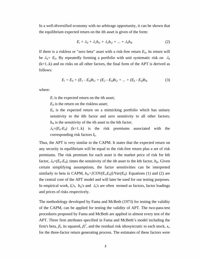
In a well-diversified economy with no arbitrage opportunity, it can be shown that the equilibrium expected return on the ith asset is given of the form:

Ei = λ0 + λ1bi1 + λ2bi2 + ... + λkbik (2)

If there is a riskless or "zero beta" asset with a risk-free return E0, its return will be λ0= E0. By repeatedly forming a portfolio with unit systematic risk on λk (k=1..k) and no risks on all other factors, the final form of the APT is derived as follows:

Ei = E0 + (E1 - E0)bi1 + (E2 - E0)bi2 + ... + (Ek - E0)bik (3)

where:

Ei is the expected return on the ith asset; E0 is the return on the riskless asset; Ek is the expected return on a mimicking portfolio which has unitary sensitivity to the kth factor and zero sensitivity to all other factors; bik is the sensitivity of the ith asset to the kth factor. λk=(Ek-E0) (k=1..k) is the risk premiums associated with the corresponding risk factors Ik.

Thus, the APT is very similar to the CAPM. It states that the expected return on any security in equilibrium will be equal to the risk-free return plus a set of risk premiums. The risk premium for each asset is the market price of risk for kth factor, λk=(Ek-E0), times the sensitivity of the ith asset to the kth factor, bjk. Given certain simplifying assumptions, the factor sensitivities can be interpreted similarly to beta in CAPM, bik=[COV(Ei,Ek)]/Var(Ek). Equations (1) and (2) are the central core of the APT model and will later be used for our testing purposes. In empirical work, Ik's, bik's and λk's are often termed as factors, factor loadings and prices of risks respectively.

The methodology developed by Fama and McBeth (1973) for testing the validity of the CAPM, can be applied for testing the validity of APT. The two-pass-test procedures proposed by Fama and McBeth are applied in almost every test of the APT. Three firm attributes specified in Fama and McBeth’s model including the firm's beta, βi, its squared, βi

2, and the residual risk idiosyncratic to each stock, si, for the three-factor return generating process. The estimates of these factors were

6

used as independent variables for the cross sectional regressions of Equation (2) to obtain time series estimates of λ1, λ2, λ3.1 The t-statistics of the mean values of these series were then tested for significant difference from zero. Based on their findings, Fama and McBeth conclude that the APT associated with the corresponding multi-factor models with the above specified factors fails to surpass the CAPM associated with the single-index model.

Because the theory does not specify which factors should be included in the APT, one may rely on certain economic beliefs when choosing the factors to perform the test. As far as macroeconomic fundamentals are concerned, the study of Bicksler (1983) made a bid to show the rationale for using the APT under uncertain inflation. Using the Fama and McBeth method, Chen, Roll and Ross (1986) based their study on certain macroeconomic forces which they believe to systematically affect the stock returns. Their findings suggest industrial production, changes in a default risk premium, term structure, and unanticipated inflation do significantly explain movement in stock prices. The striking result is that when accompanying other economic forces, the stock market index fails to have significant effect on stock returns.

On the other hand, Chan Hamao, and Lakonishok (1991) relate the stock prices to microeconomic fundamentals, say, earning yield, size, book to market ratio, and cash flow yield. All four variables, of which book to market ratio and cash flow yield had the most significant positive impact, were proved to systematically affect the expected stock returns.

While the approach is convincing, doubts are cast over the rationale of economic variables that are chosen as factors Ik's. The question is whether one should rely either entirely or partly on the basis of theory or on the empirical evidence when choosing these factors. Empirical evidence would be persuasive, but without a theory, the results would be difficult to interpret.

3. Methodology and Data Selection:

The principle of the methodology for testing the APT in the Stock Exchange of

1 Details of the procedures are the same as what we will describe in the fourth section of our paper.

7

Thailand (SET) heavily relies on the method suggested by Fama and McBeth (1973) since it is not deniable that the method has been intensively applied by many academics such as Brown and Weinstein (1983), Chen (1983), Chen, Roll and Ross (1986), and Chan, Hamao and Lakonishok (1991). These authors are named for their approaches to the problem are also particularly useful for the testing models of this paper.

Equation (1) and (2) mentioned in Section 2 are the central equations of this test. For demonstration purposes, the equations will shortly be reproduced in slightly different notations in such a way that are appropriate for following the test of this paper. The original return generating process of 67 individual equities listed on the Stock Exchange of Thailand collected for the test are assumed to be:

~ ~ ~R E Iit i ik ktk

j

i= + +=∑β ε

1 (i=1..67; j=1,3,5,7) (4)

where ~Rit is the return on the ith stock at time t; Ei is the expected return on the ith stock; ~I kt is the mean-zero kth factor common to all assets, ~I kt can vary stochatistically from period to period; β ik is the sensitivity of the return on the ith stock to unexpected changes in the kth factor; and ~εi is the nonsystematic risk

component specific to the ith stock which is identically independently distributed with zero mean E( ~εi | ~I kt )=0 for all k; j receives either one of the value of the set

of [1, 3, 5, 7], i.e. we will test for the appropriate return generating process of single-factor, 3-factor, 5-factor and 7-factor models. The choice of 7 as the maximum number of factors is associated with the previous work by Elton and Gruber (1984). However, it can be predicted that too many variables to be included in a model would reduce the precision of the estimates as the disturbance terms of different variables may cancel out the effects of other variables. In view of the fact that the data are only rich enough for us to observe our variables in very short period from 1987-1996, we cannot carry out the test in different period to observe whether it follows a consistent pattern. Instead, we have no choice but to perform some conceivable models and check their consistent properties. To that end, we step by step reduce the number of factors to be included in our models. The choice of odd number of factors is simply to save cost of calculation. Five- factor models are claimed to be enough by Roll and Ross (1980), Chen (1983), Chen, Roll and Ross (1986). Three-factor models

8

are suggested to use by Brown and Weinstein (1983). Single factor models are needed to test the CAPM.

Using portfolios instead of individual securities would obviously increase the precision of the obtained estimates1. The problems are how to group portfolios so that we can optimally reduce the loss of information and/or eliminate regression phenomenon caused by using portfolios rather than individual securities. Fama and McBeth (1973: 615) proposed to use the estimates of βik from the previous

time to rank the securities into portfolios for the subsequent period test. However Chen, Roll and Ross (1986) made a number of experiments to rank the securities according to (a) the estimatedβ i ; (b) the estimated standard deviation σ i of the

market-model regression; and (c) the level of the stock price; and claimed the market value of the firm is the best criterion for dividing securities into portfolios. 67 securities are therefore grouped into 17 equally weighted portfolios of 4 stocks each (except the last portfolio which has only 3 stocks) according to their market value on 31 January 19872.

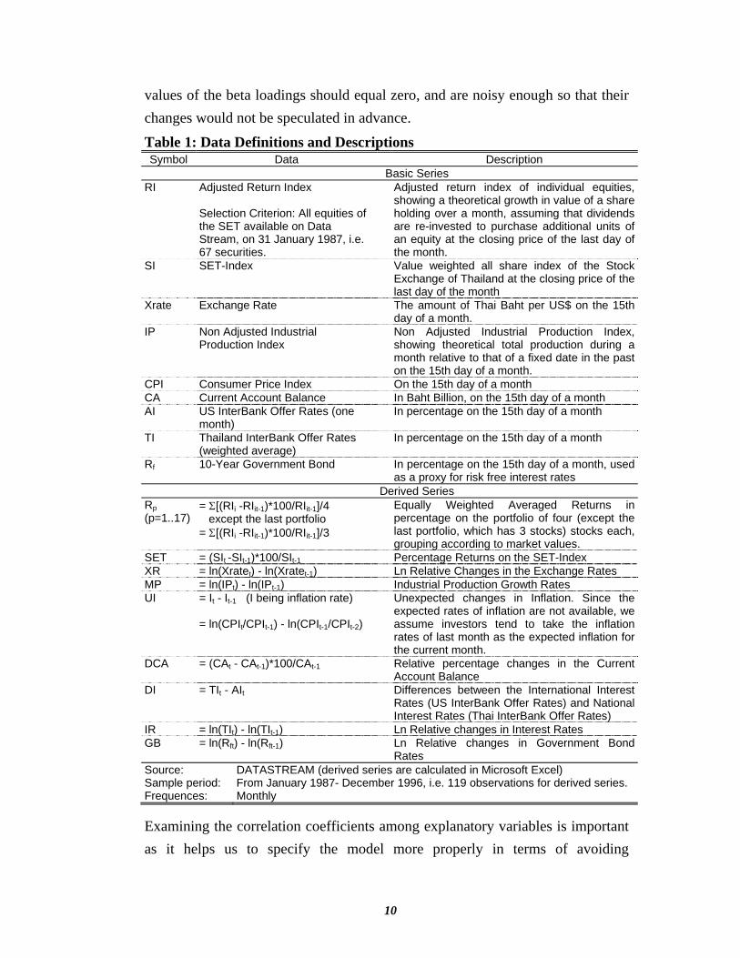
The variables chosen for this test are based on the evidence of previous research on the APT and the above mentioned characteristics of the SET. Table 1 lists all the variables used in this research with their descriptions. All the data have been downloaded from DataStream for the period between January 1987 and December 1996. Longer period would have been better for the test, but there are not so much choice. As noted above, the dim period before 1987 did not see so much trading in the SET. The period of crisis in 1997-1998 should obviously be excluded as non-fundamental price behaviour can be foreseen. On the condition of sufficient observations, the longer the time span between observations is, the more precise the estimates are since general trend can be captured why eliminating the short-run unsystematic deviation in stock behaviour; hence monthly data are chosen.

The estimates of betas will be more precise if as many equities as possible are employed. Unfortunately, in the emerging market, this requirement is hardly met.

1 See Fama and McBeth (1973: 614) for a simple proof. 2 It would be more desirable if experiment on grouping portfolios according to their previous etimated betas could be carried out. However, as noted above, the sample period is too short to do so.

9

Although, data for all stocks available on Data Stream for January 31, 1987 have been collected, the total testing stocks can only make up the maximum figure of 67. The monthly returns on SET-Index used as the proxy of the returns on market portfolios, which are usually included in the stock research, are by no means excluded from the testing models.

Other economic variables such as industrial production, proved to have explanatory power on stock return by Chen, Roll and Ross (1986), and unexpected inflation, used by Chen Roll and Ross (1986) and Bicksler (1983), are present in the testing models. To qualify for the mean zero requirement of the explaining factors, the monthly growth rates of industrial production and the unexpected inflation rates are used.

The changes in risky interest rates employed are the monthly logarithmic relative changes in the Thailand InterBank Offer Rates (weighted average). The riskless interest rates applied are the 10 Year Government Bond Rates. Given the Thai economy, in general, and the SET performance, in particular, are susceptibly vulnerable to external shocks, we have included three economic indicators to reflect the impact of external factors. They are the international interest rates (One month US InterBank Offer Rates1 are used as the proxy), the Baht-USD exchange rates, and the Current Account Balance under Thailand's Balance of Payment. Since Thai risky interest rates are highly correlated to the US ones2, we use the percentage difference between the two rates, denoted as DI. The rates of changes in exchange rates are in natural logarithm, while the rates of changes in Current Account Balance are in percentage changes to allow for the fact that the balance can well be either positive or negative.

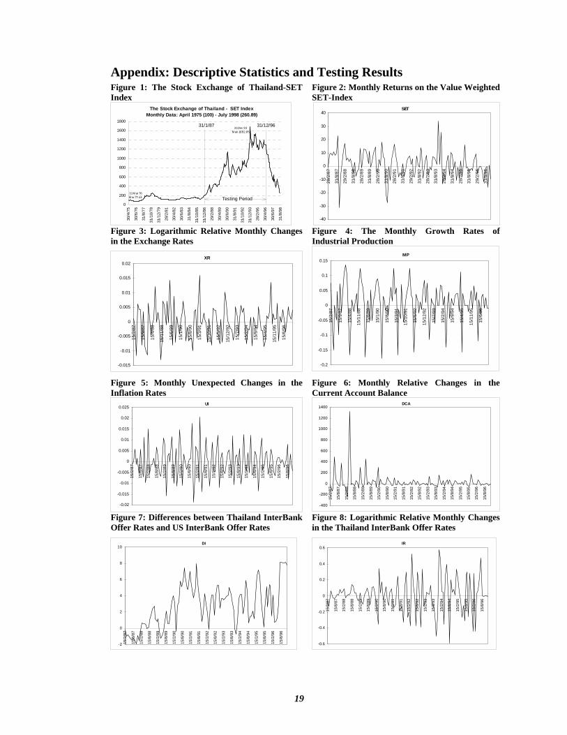
The Appendix presents the graphs of our derived economic variables, some of which will be included in our testing model. Apart from the fact that DI tends to diverge from the horizontal axis and GB is so persistent to change, all other variables seem to satisfy the first requirement of the APT model, i.e. the expected

1 It would be ideal if we could get the International Interest Rate proxy of the same due period as the Domestic Interest Rate proxy. However, there are no such data available in DataStream for Thailand. 2 In fact, when we try using both Thailand and US InterBank rates, regressions in Microfit are forbidden because of multicolinearity.

10

values of the beta loadings should equal zero, and are noisy enough so that their changes would not be speculated in advance. Table 1: Data Definitions and Descriptions Symbol Data Description

Basic Series RI Adjusted Return Index

Selection Criterion: All equities of the SET available on Data Stream, on 31 January 1987, i.e. 67 securities.

Adjusted return index of individual equities, showing a theoretical growth in value of a share holding over a month, assuming that dividends are re-invested to purchase additional units of an equity at the closing price of the last day of the month.

SI SET-Index Value weighted all share index of the Stock Exchange of Thailand at the closing price of the last day of the month

Xrate Exchange Rate The amount of Thai Baht per US$ on the 15th day of a month.

IP Non Adjusted Industrial Production Index

Non Adjusted Industrial Production Index, showing theoretical total production during a month relative to that of a fixed date in the past on the 15th day of a month.

CPI Consumer Price Index On the 15th day of a month CA Current Account Balance In Baht Billion, on the 15th day of a month AI US InterBank Offer Rates (one

month) In percentage on the 15th day of a month

TI Thailand InterBank Offer Rates (weighted average)

In percentage on the 15th day of a month

Rf 10-Year Government Bond In percentage on the 15th day of a month, used as a proxy for risk free interest rates

Derived Series Rp (p=1..17)

= Σ[(RIi -RIit-1)*100/RIit-1]/4 except the last portfolio = Σ[(RIi -RIit-1)*100/RIit-1]/3

Equally Weighted Averaged Returns in percentage on the portfolio of four (except the last portfolio, which has 3 stocks) stocks each, grouping according to market values.

SET = (SIt -SIt-1)*100/SIt-1 Percentage Returns on the SET-Index XR = ln(Xratet) - ln(Xratet-1) Ln Relative Changes in the Exchange Rates MP = ln(IPt) - ln(IPt-1) Industrial Production Growth Rates UI = It - It-1 (I being inflation rate)

= ln(CPIt/CPIt-1) - ln(CPIt-1/CPIt-2)

Unexpected changes in Inflation. Since the expected rates of inflation are not available, we assume investors tend to take the inflation rates of last month as the expected inflation for the current month.

DCA = (CAt - CAt-1)*100/CAt-1 Relative percentage changes in the Current Account Balance

DI = TIt - AIt Differences between the International Interest Rates (US InterBank Offer Rates) and National Interest Rates (Thai InterBank Offer Rates)

IR = ln(TIt) - ln(TIt-1) Ln Relative changes in Interest Rates GB = ln(Rft) - ln(Rft-1) Ln Relative changes in Government Bond

Rates Source: DATASTREAM (derived series are calculated in Microsoft Excel) Sample period: From January 1987- December 1996, i.e. 119 observations for derived series. Frequences: Monthly

Examining the correlation coefficients among explanatory variables is important as it helps us to specify the model more properly in terms of avoiding

11

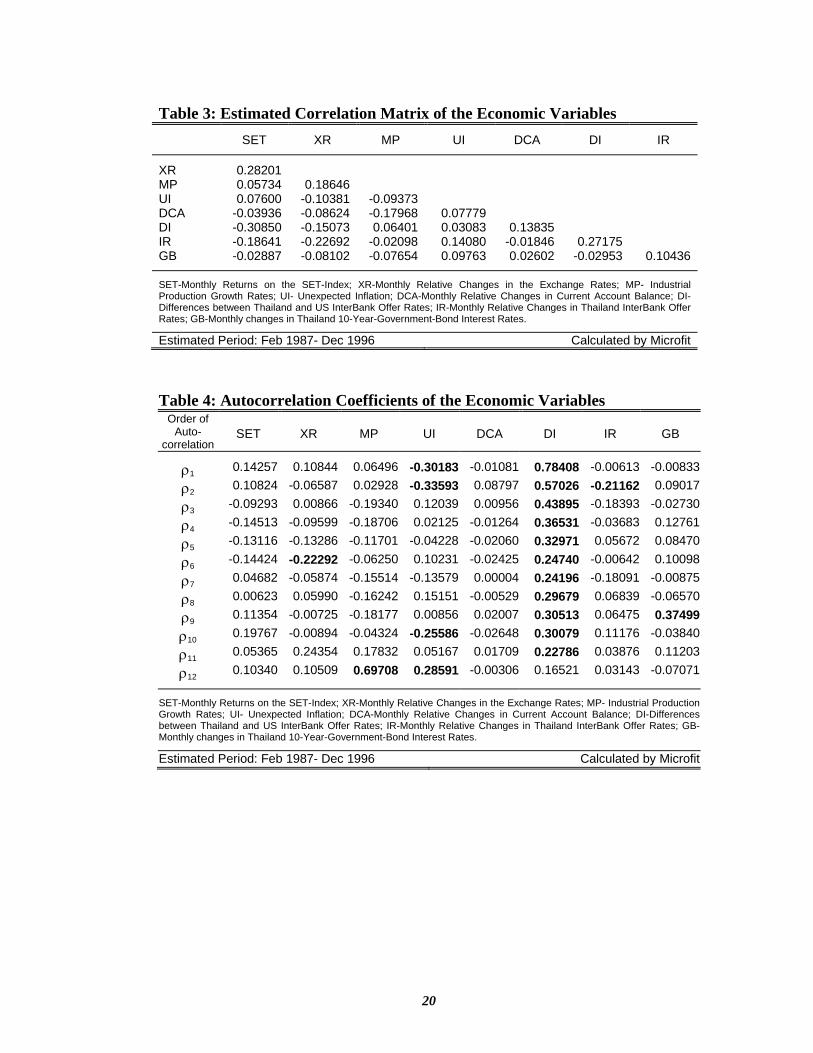
multicolinearity which would result in unreliable statistical inference (Gujarati 1995). The correlation matrix of the derived economic variables is produced in Table 3 in Appendix. XR is correlated with all other variables but DCA and GB, which promises the possibility of inclusion of XR in the model might also imply the exclusion of some others. However, this possibility is not very strong since all the correlation is less than 0.3. The strongest correlation is between SET and DI, SET and XR, and IR and DI for the reasons which can be predicted: Returns on the constituent stocks of SET are exposed to external shocks and DI is the difference between the two highly correlated series AI and TI which makes IR. Other correlations exist between SET and IR, MP and UI, UI and IR, DCA and DI, and IR and GB. The presence of correlations between explaining variables presages that model specification should be handled with care. However, the correlations between variables are far from perfect.

The table immediately following the table of correlation matrix, Table 4, notes the autocorelation of the economic variables from order 1 to 12. Generally, autocorrelations will not be a serious problem for the precision of our estimates, since they are fairly modest. DI is the most highly autocorrelated, warning it pays attention. MP displays the highest serial correlation in its lag at 12 months, informing of seasonal characteristics. Other high autocorrelations are associated with UI, XR and IR. It would be meaningful to note that in the presence of autocorrelation, Ordinary Least Square (OLS) estimators are still unbiased and consistent, but they are no longer efficient, i.e. minimum variance (Gujarati 1995). Thus, the significance of our test will be biased downward.

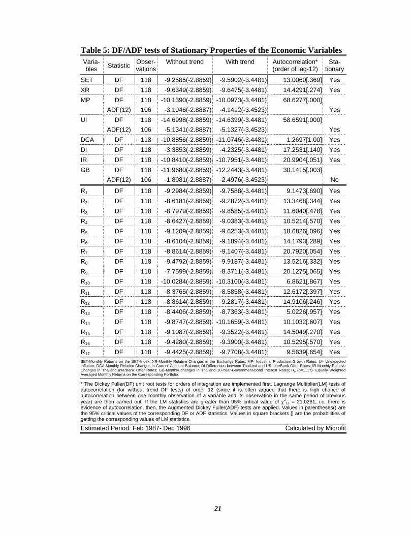
The stationary properties of employed variables are finally examined as it is often argued that regressions between nonstationary variables would be spurious, and the results are of no use. The Dickey Fuller (DF) unit roots tests (and where necessary1) Augmented Dickey Fuller (ADF) tests are applied to those variables. Fortunately, almost all these variables are immune from nonstationary process I(1), but GB. This is not very surprising, however, because in manipulating the variables to suit the requirement of the zero-mean factors of the APT, most of

1 When the DF test shows evidence of autocorrelation of a particular order, the ADF test will then enter the tournament to test for the stationary properties of the economic series at the corresponding order of autocorrelation.

12

these variables are already in the form of first differences. The stationary properties of these variables are essential for this test. It will significantly increase the precision of the estimates and the reliability of the tests.

The test then is implemented following the procedures:

1. Using the data of the previous five years (i.e. 1987-1991) of the subsequent year's (1992) regressions mentioned in the second step, each portfolio's sensitivities, β pk 's, to unanticipated changes in the economic factors, ~I kt 's, are

estimated by regressing the equally weighted portfolio's returns on the factors, using the following models where p denotes portfolios:

R Ipt p pk ktk

j

p= + +=∑α β ε~

1 (p=1..17; j=1,3,5,7; t=1..60, except 1987) (5)

2. Estimating the risk premia,λ k 's, for each associated factor, by running 12

cross-sectional regressions of the 17 portfolios' returns for each month of the subsequent year (1992) on the estimates of the factor loadings or betas, β pk 's,

obtained from the first step:

Rpt k pkk

j

t= + +=∑λ λ β ω0

1 (p=1..17; j=1,3,5,7; t=1..12) (6)

where λk's denoted the risk premia associated with the kth factor. Thus, series of 12 estimates of the risk premia of each factor, λ k , for the year (1992) will be

obtained.

3. The first and second steps are then repeated for the year 1991-1996. Thus, 59 observations (Feb 1987-Dec 1991) are used to obtain β pk 's. Then, 17 observations

of the portfolios' returns for each month of 1992 and the resulting β pk 's are used to

get a time series of 12 λ k for each factor. In subsequent periods, namely, Jan 1988-

Dec 1992; Jan 1989-Dec 1993; Jan 1990-Dec 1994; Jan 1991-Dec 1995; 60 observations are used to obtain β pk 's. Then, the same as the year 1992, a time series

of 12 λ k for each factor is attained for each year from 1993-1996.

13

4. The time series mean of 60 estimates of the risk premium of each factor, λ k ,

are tested for the null hypothesis of λ k = 0, using the t-statistics1:

ts nk

k

k

( )( ) /

λλ

λ= (7)

Where n=60 is the number of the months from Jan 1992-Dec 1996, which is also the number of estimates λ k used to compute λ k and s(λ k ).

At this stage, it is worth mentioning some errors-in-variables problems, that would challenge the desirability of our method. As in the second step of cross-sectional regressions, it would be desirable if we had the true βpk's to estimate the risk primia. However, it is hardly the case, so estimated β pk 's are used instead.

β pk 's themselves are measured with errors, and our estimates of risk primia,λ k 's

would, therefore, be much less precise if true βpk's are used. Fortunately, Elton and Gruber (1995: 349) show that when betas are estimated for portfolios, random errors in measuring individual stocks' betas will cancel out and the aggregate error will be very small.

Another problem is the distortion in the existence of heteroscedasticity, i.e. higher betas have higher variance of returns, that would bias downwards the estimates of the regression variance and would be more likely to lead us to the conclusion of statistical significant relation when, in fact, it is not. This fact should be noted for later interpretation. However, as stocks are grouped into portfolios according to the market values, true betas would spread between portfolios and reduce the problem substantially. In fact, the "White's general heteroscedasticity test" and the "Breusch-Pagan-Godfrey test" of heteroscedasticity" (Gujarati 1995: 377-380) were carried out in Microfit on the random basis2 for the testing sample and found that the sample poses no serious problems of heteroscedasticity.

1 See Fama and McBeth (1973: 619) for details of the properties of the statistics. 2 It is impossible for us to carry out the tests for every regression since the total number of our regressions would be well above 1300 (only basic regressions are counted).

14

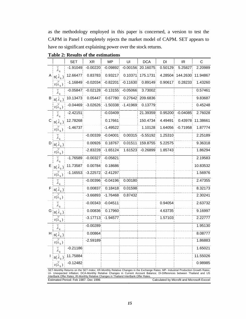
4. Testing Results

Table 2 reports the results obtained by applying the methodology in question to the Stock Exchange of Thailand for the period between 1987 and 1996. Panel A shows the result of applying the 7-factor model. No factors appear to explain the asset returns on the SET. Perhaps, as predicted above, that is because too many variables to be included in the model would cancel out the effects of one another. The low insignificant factor, RI, is then deleted but UI and XR are still retained for the above discussion of the SET supports the price explanatory power of unexpected changes in inflation and changes in exchange rates. DI is deleted because, as noted above, its properties do not really qualify for the APT model. The result appears in Panel B is more persuasive. The most insignificant factor turns out to be the significant one, i.e. the changes in exchange rates, other factors remain insignificant. However, we this result is not immediately relied on and further tests are implemented.

In view of relatively high t-value of the difference between domestic interest rates and international interest rates, DI, may imply its price explaining power, the test in Panel C is carried out, but this time, the lowest significant factors MP and UI are deleted. The result supports our view, no factors seem to be significant. The last test for five-factor model is then performed, canceling the market factor SET, as it appears to be consistently insignificant. Much of the t-values of the associated factors are improved with XR remains highly significant and DI marginally insignificant.

With a view to avoiding data mining further tests to check the consistent significance of XR are implemented. Three-factor models now come into play. The first test reported in Panel E shows one more significant factor, MP. Deleting the SET and adding UI improves the significance of XR but worsens the support for MP in Panel F. When DI is included in Panel G, it weakens the significance of XR, and the factor itself is insignificant.

Finally, the single model test for the consistent significant factor, XR, and the market-model, CAPM are performed. Once again the result in Panel H supports that XR is consistently significant over the selected models, except the 7-factor model as it is too noisy and XR is correlated with many of those explanatory variables. As far

15

as the methodology employed in this paper is concerned, a version to test the CAPM in Panel I completely rejects the market model of CAPM. SET appears to have no significant explaining power over the stock returns.

Table 2: Results of the estimations SET XR MP UI DCA DI IR C λ k -1.91049 -0.00220 -0.09892 -0.00156 20.16075 0.50129 5.25827 2.20989

A s( λ k ) 12.66477 0.83783 0.93217 0.10371 175.1731 4.28504 144.2630 11.94867

t k( )λ -1.16849 -0.02034 -0.82201 -0.11630 0.89149 0.90617 0.28233 1.43260

λ k -0.05847 -0.02128 -0.13155 -0.05066 3.73002 0.57461

B s( λ k ) 10.13473 0.05447 0.67780 0.27642 209.6836 9.83687

t k( )λ -0.04469 -3.02626 -1.50338 -1.41969 0.13779 0.45248

λ k -2.42151 -0.03409 21.39359 0.95200 -0.04085 2.76028

C s( λ k ) 12.78268 0.17661 150.4734 4.49491 0.43978 11.38661

t k( )λ -1.46737 -1.49522 1.10128 1.64056 -0.71958 1.87774

λ k -0.00339 -0.04001 0.00315 -5.55192 1.25310 2.25189

D s( λ k ) 0.00926 0.18767 0.01511 159.8755 5.22575 9.36318

t k( )λ -2.83228 -1.65124 1.61523 -0.26899 1.85743 1.86294

λ k -1.76589 -0.00327 -0.05821 2.19583

E s( λ k ) 11.73587 0.00784 0.18686 10.83532

t k( )λ -1.16553 -3.22572 -2.41297 1.56976

λ k -0.00396 -0.04196 0.00180 2.47355

F s( λ k ) 0.00837 0.18418 0.01598 8.32173

t k( )λ -3.66893 -1.76468 0.87432 2.30241

λ k -0.00343 -0.04511 0.94054 2.63732

G s( λ k ) 0.00836 0.17960 4.63735 9.16997

t k( )λ -3.17713 -1.94577 1.57103 2.22777

λ k -0.00289 1.95130

H s( λ k ) 0.00864 8.08777

t k( )λ -2.59189 1.86883

λ k -0.21186 1.65021

I s( λ k ) 11.75884 11.55026

t k( )λ -0.12482 0.98985

SET-Monthly Returns on the SET-Index; XR-Monthly Relative Changes in the Exchange Rates; MP- Industrial Production Growth Rates; UI- Unexpected Inflation; DCA-Monthly Relative Changes in Current Account Balance; DI-Differences between Thailand and US InterBank Offer Rates; IR-Monthly Relative Changes in Thailand InterBank Offer Rates.Estimated Period: Feb 1987- Dec 1996 Calculated by Microfit and Microsoft Exccel

16

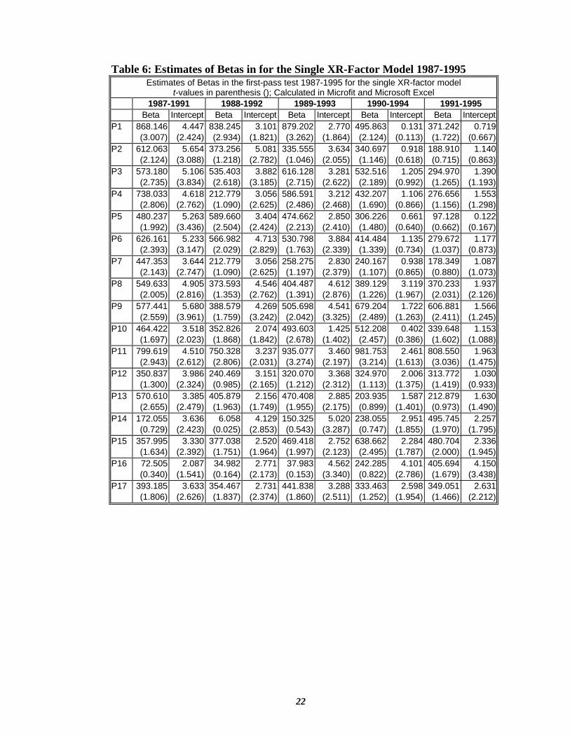
Estimating the values of betas using equation (1) in the first-pass test are the most important and the central question of corporate finance, for it is the basis of the decision making process to observe and predict changes in the company's stock behaviour responding to the movement of corresponding factors (macroeconomic fundamentals in this paper's case), so that well preparation can be made, and hence proper performance results. However, deriving the risk premia associated with those factors using equation (2) in the second-pass test is essential to finance academics and practitioners since it provides estimates of unobserved indicators, the investors' sentiment toward risks of changes in those factors and how they price risks accordingly so that it can confirms the reliability of the beta estimates obtained in the first pass test. This research, however, pays attention to the market as a whole and studies the general behaviour of all stocks towards innovations. For that reason, the beta estimates obtained in the first pass test are not produced except the betas of changes in the exchange rate, XR, in the single XR-factor model (see Appendix). Furthermore, the number of regressions does not allow us to do so.

If the employed sample does properly reflect the behaviour of all the stock at least for the observed period1, some conclusions can be derived from this study as follows. The behaviour of stock price movement completely denies the existence of 7 factors model. The changes in exchange rates are consistently priced and there is one chance (see the three-factor model in Panel E) that the industrial growth rates are priced.

The negative significant estimates of risk primia and the positive values of betas for XR may show that people tend to price the stock, whose sensitivity to changes in exchange rates is high, relatively lower than the stock, whose sensitivity to changes in exchange rate is low. This may imply people are risk-averse and they do not want the fluctuation of stock price towards risks of changes in exchange rates, hence they tend to hedge against such changes.

If the only chance of significance of the industrial growth rates happens to be correct2, the negative risk premium estimates of the industrial production growth

1 Note the error-in-variables problem mentioned above. 2 It is hard to believe it is true.

17

rates are strange because they are usually positive1, and can be interpreted in the same way as the exchange rate. Although, the general trend of the annual industrial production growth rates is positively high, the monthly growth rates, affected by the seasonal factor, are noisy enough for risk-averse investors to have a tendency to hedge. Therefore, the more sensitive to the monthly growth rates a stock is, the lower price it receives.

Of the factors that are observed not to be priced, including the returns on the market portfolio, the unexpected changes in inflation, the relative changes in the current account balance, the changes in domestic interest rate, and the difference between domestic interest rates and the international interest rates; the insignificance of the returns on market portfolio, SET, is the most striking since its explanatory power in the first-pass test is relatively high. However, this can be explained that the high correlation with the stock returns in the first pass test is because the stock itself is a constituent of the SET-Index. The second pass test confirms people do not price risks of changes in the index's returns.

5. Conclusion

Using the method suggested by Fama and McBeth (1973), this research has examined the stock price behaviour in an emerging stock market, the SET. Although, the findings may be affected from thin data base of the stock profile, since only 67 available stocks are investigated. The results obtained may be persuasive. On the basis of available data, the findings confirm that the stock price of the newly established market of Thailand does conform with the inspiration of the APT. At least one factor, the logarithmic relative changes in the exchange rates, and two factors for a chance, the mentioned factor and the industrial growth rates, do systematically explain the stock prices. Within the scope of this paper's methodology, the returns on the market portfolio and the single market model of CAPM do not hold.

The findings of this paper are important for finance academics and practitioners. At least, to some extent, financial practitioners can refer to this study for their policy making process as the APT can be used as a tool of investment analysis even in an emerging stock market such as Thailand. So few macroeconomic fundamental

1 For example in the work of Chen, Roll and Ross (1986)

18

factors priced may imply the immaturity of the SET, and also the low degree of financial liberalisation in Thailand as policy makers are reluctant to trade off the stability and efficiency. However, efficiency is the key to stability, and stability forced artificially by policy makers will finally turn out to be turmoil and result in crises. Therefore, policy makers, while trying to maintain the market stability and remedying market failures, should place an appropriate balance to market efficiency. The higher degree of financial liberalisation may lead to more fundamental relationship between stock prices and economic factors and that is the basis of stability.

This research contributes to the APT literature in the emerging stock markets. The immature SET is only observed for a very short period of time before the Asian Financial Crisis. However, the research methodology is open for the judgment of further study in the field about its appropriateness for emerging markets. At least, a suggestion for further research can be made is to apply the same methodology for the period after the Crisis, so that it general behaviour can be observed.

19

Appendix: Descriptive Statistics and Testing Results Figure 1: The Stock Exchange of Thailand-SET Index

The Stock Exchange of Thailand - SET IndexMonthly Data: April 1975 (100) - July 1998 (260.89)

0

200

400

600

800

1000

1200

1400

1600

1800

30/4

/75

30/6

/76

31/8

/77

31/1

0/78

31/1

2/79

28/2

/81

30/4

/82

30/6

/83

31/8

/84

31/1

0/85

31/1

2/86

29/2

/88

30/4

/89

30/6

/90

31/8

/91

31/1

0/92

31/1

2/93

28/2

/95

30/4

/96

30/6

/97

31/8

/98

31/1/87 31/12/96

Testing Period31 M ar 76M in-77.44

31 Dec 93M ax-1682.85

Figure 2: Monthly Returns on the Value Weighted SET-Index

SET

-40

-30

-20

-10

0

10

20

30

40

28/2

/87

31/8

/87

29/2

/88

31/8

/88

28/2

/89

31/8

/89

28/2

/90

31/8

/90

28/2

/91

31/8

/91

29/2

/92

31/8

/92

28/2

/93

31/8

/93

28/2

/94

31/8

/94

28/2

/95

31/8

/95

29/2

/96

31/8

/96

Figure 3: Logarithmic Relative Monthly Changes in the Exchange Rates

XR

-0.015

-0.01

-0.005

0

0.005

0.01

0.015

0.02

15/2

/87

15/9

/87

15/4

/88

15/1

1/88

15/6

/89

15/1

/90

15/8

/90

15/3

/91

15/1

0/91

15/5

/92

15/1

2/92

15/7

/93

15/2

/94

15/9

/94

15/4

/95

15/1

1/95

15/6

/96

Figure 4: The Monthly Growth Rates of Industrial Production

MP

-0.2

-0.15

-0.1

-0.05

0

0.05

0.1

0.15

15/2

/87

15/9

/87

15/4

/88

15/1

1/88

15/6

/89

15/1

/90

15/8

/90

15/3

/91

15/1

0/91

15/5

/92

15/1

2/92

15/7

/93

15/2

/94

15/9

/94

15/4

/95

15/1

1/95

15/6

/96

Figure 5: Monthly Unexpected Changes in the Inflation Rates

UI

-0.02

-0.015

-0.01

-0.005

0

0.005

0.01

0.015

0.02

0.025

15/2

/87

15/8

/87

15/2

/88

15/8

/88

15/2

/89

15/8

/89

15/2

/90

15/8

/90

15/2

/91

15/8

/91

15/2

/92

15/8

/92

15/2

/93

15/8

/93

15/2

/94

15/8

/94

15/2

/95

15/8

/95

15/2

/96

15/8

/96

Figure 6: Monthly Relative Changes in the Current Account Balance

DCA

-400

-200

0

200

400

600

800

1000

1200

1400

15/2

/87

15/8

/87

15/2

/88

15/8

/88

15/2

/89

15/8

/89

15/2

/90

15/8

/90

15/2

/91

15/8

/91

15/2

/92

15/8

/92

15/2

/93

15/8

/93

15/2

/94

15/8

/94

15/2

/95

15/8

/95

15/2

/96

15/8

/96

Figure 7: Differences between Thailand InterBank Offer Rates and US InterBank Offer Rates

DI

-2

0

2

4

6

8

10

15/2

/87

15/8

/87

15/2

/88

15/8

/88

15/2

/89

15/8

/89

15/2

/90

15/8

/90

15/2

/91

15/8

/91

15/2

/92

15/8

/92

15/2

/93

15/8

/93

15/2

/94

15/8

/94

15/2

/95

15/8

/95

15/2

/96

15/8

/96

Figure 8: Logarithmic Relative Monthly Changes in the Thailand InterBank Offer Rates

IR

-0.6

-0.4

-0.2

0

0.2

0.4

0.6

15/2

/87

15/8

/87

15/2

/88

15/8

/88

15/2

/89

15/8

/89

15/2

/90

15/8

/90

15/2

/91

15/8

/91

15/2

/92

15/8

/92

15/2

/93

15/8

/93

15/2

/94

15/8

/94

15/2

/95

15/8

/95

15/2

/96

15/8

/96

20

Table 3: Estimated Correlation Matrix of the Economic Variables

SET XR MP UI DCA DI IR

XR 0.28201 MP 0.05734 0.18646 UI 0.07600 -0.10381 -0.09373 DCA -0.03936 -0.08624 -0.17968 0.07779 DI -0.30850 -0.15073 0.06401 0.03083 0.13835 IR -0.18641 -0.22692 -0.02098 0.14080 -0.01846 0.27175 GB -0.02887 -0.08102 -0.07654 0.09763 0.02602 -0.02953 0.10436

SET-Monthly Returns on the SET-Index; XR-Monthly Relative Changes in the Exchange Rates; MP- Industrial Production Growth Rates; UI- Unexpected Inflation; DCA-Monthly Relative Changes in Current Account Balance; DI-Differences between Thailand and US InterBank Offer Rates; IR-Monthly Relative Changes in Thailand InterBank Offer Rates; GB-Monthly changes in Thailand 10-Year-Government-Bond Interest Rates.

Estimated Period: Feb 1987- Dec 1996 Calculated by Microfit

Table 4: Autocorrelation Coefficients of the Economic Variables Order of

Auto-correlation

SET

XR

MP

UI

DCA

DI

IR

GB

ρ1 0.14257 0.10844 0.06496 -0.30183 -0.01081 0.78408 -0.00613 -0.00833

ρ2 0.10824 -0.06587 0.02928 -0.33593 0.08797 0.57026 -0.21162 0.09017

ρ3 -0.09293 0.00866 -0.19340 0.12039 0.00956 0.43895 -0.18393 -0.02730

ρ4 -0.14513 -0.09599 -0.18706 0.02125 -0.01264 0.36531 -0.03683 0.12761

ρ5 -0.13116 -0.13286 -0.11701 -0.04228 -0.02060 0.32971 0.05672 0.08470

ρ6 -0.14424 -0.22292 -0.06250 0.10231 -0.02425 0.24740 -0.00642 0.10098

ρ7 0.04682 -0.05874 -0.15514 -0.13579 0.00004 0.24196 -0.18091 -0.00875

ρ8 0.00623 0.05990 -0.16242 0.15151 -0.00529 0.29679 0.06839 -0.06570

ρ9 0.11354 -0.00725 -0.18177 0.00856 0.02007 0.30513 0.06475 0.37499ρ10 0.19767 -0.00894 -0.04324 -0.25586 -0.02648 0.30079 0.11176 -0.03840

ρ11 0.05365 0.24354 0.17832 0.05167 0.01709 0.22786 0.03876 0.11203

ρ12 0.10340 0.10509 0.69708 0.28591 -0.00306 0.16521 0.03143 -0.07071

SET-Monthly Returns on the SET-Index; XR-Monthly Relative Changes in the Exchange Rates; MP- Industrial Production Growth Rates; UI- Unexpected Inflation; DCA-Monthly Relative Changes in Current Account Balance; DI-Differences between Thailand and US InterBank Offer Rates; IR-Monthly Relative Changes in Thailand InterBank Offer Rates; GB-Monthly changes in Thailand 10-Year-Government-Bond Interest Rates.

Estimated Period: Feb 1987- Dec 1996 Calculated by Microfit

21

Table 5: DF/ADF tests of Stationary Properties of the Economic Variables Varia-bles Statistic Obser-

vations Without trend With trend Autocorrelation*

(order of lag-12) Sta-

tionary

SET DF 118 -9.2585(-2.8859) -9.5902(-3.4481) 13.0060[.369] Yes XR DF 118 -9.6349(-2.8859) -9.6475(-3.4481) 14.4291[.274] Yes MP DF 118 -10.1390(-2.8859) -10.0973(-3.4481) 68.6277[.000] ADF(12) 106 -3.1046(-2.8887) -4.1412(-3.4523) Yes UI DF 118 -14.6998(-2.8859) -14.6399(-3.4481) 58.6591[.000] ADF(12) 106 -5.1341(-2.8887) -5.1327(-3.4523) Yes DCA DF 118 -10.8856(-2.8859) -11.0746(-3.4481) 1.2697[1.00] Yes DI DF 118 -3.3853(-2.8859) -4.2325(-3.4481) 17.2531[.140] Yes IR DF 118 -10.8410(-2.8859) -10.7951(-3.4481) 20.9904[.051] Yes GB DF 118 -11.9680(-2.8859) -12.2443(-3.4481) 30.1415[.003] ADF(12) 106 -1.8081(-2.8887) -2.4976(-3.4523) No

R1 DF 118 -9.2984(-2.8859) -9.7588(-3.4481) 9.1473[.690] Yes R2 DF 118 -8.6181(-2.8859) -9.2872(-3.4481) 13.3468[.344] Yes R3 DF 118 -8.7979(-2.8859) -9.8585(-3.4481) 11.6040[.478] Yes R4 DF 118 -8.6427(-2.8859) -9.0383(-3.4481) 10.5214[.570] Yes R5 DF 118 -9.1209(-2.8859) -9.6253(-3.4481) 18.6826[.096] Yes R6 DF 118 -8.6104(-2.8859) -9.1894(-3.4481) 14.1793[.289] Yes R7 DF 118 -8.8614(-2.8859) -9.1407(-3.4481) 20.7920[.054] Yes R8 DF 118 -9.4792(-2.8859) -9.9187(-3.4481) 13.5216[.332] Yes R9 DF 118 -7.7599(-2.8859) -8.3711(-3.4481) 20.1275[.065] Yes R10 DF 118 -10.0284(-2.8859) -10.3100(-3.4481) 6.8621[.867] Yes R11 DF 118 -8.3765(-2.8859) -8.5858(-3.4481) 12.6172[.397] Yes R12 DF 118 -8.8614(-2.8859) -9.2817(-3.4481) 14.9106[.246] Yes R13 DF 118 -8.4406(-2.8859) -8.7363(-3.4481) 5.0226[.957] Yes R14 DF 118 -9.8747(-2.8859) -10.1659(-3.4481) 10.1032[.607] Yes R15 DF 118 -9.1087(-2.8859) -9.3522(-3.4481) 14.5049[.270] Yes R16 DF 118 -9.4280(-2.8859) -9.3900(-3.4481) 10.5295[.570] Yes R17 DF 118 -9.4425(-2.8859) -9.7708(-3.4481) 9.5639[.654] Yes SET-Monthly Returns on the SET-Index; XR-Monthly Relative Changes in the Exchange Rates; MP- Industrial Production Growth Rates; UI- Unexpected Inflation; DCA-Monthly Relative Changes in Current Account Balance; DI-Differences between Thailand and US InterBank Offer Rates; IR-Monthly Relative Changes in Thailand InterBank Offer Rates; GB-Monthly changes in Thailand 10-Year-Government-Bond Interest Rates; Rp (p=1..17)- Equally Weighted Averaged Monthly Returns on the Corresponding Portfolio.

* The Dickey Fuller(DF) unit root tests for orders of integration are implemented first. Lagrange Multiplier(LM) tests of autocorrelation (for without trend DF tests) of order 12 (since it is often argued that there is high chance of autocorrelation between one monthly observation of a variable and its observation in the same period of previous year) are then carried out. If the LM statistics are greater than 95% critical value of χ2

12 = 21.0261, i.e. there is evidence of autocorrelation, then, the Augmented Dickey Fuller(ADF) tests are applied. Values in parentheses() are the 95% critical values of the corresponding DF or ADF statistics. Values in square brackets [] are the probabilities of getting the corresponding values of LM statistics.

Estimated Period: Feb 1987- Dec 1996 Calculated by Microfit

22

Table 6: Estimates of Betas in for the Single XR-Factor Model 1987-1995 Estimates of Betas in the first-pass test 1987-1995 for the single XR-factor model

t-values in parenthesis (); Calculated in Microfit and Microsoft Excel 1987-1991 1988-1992 1989-1993 1990-1994 1991-1995 Beta Intercept Beta Intercept Beta Intercept Beta Intercept Beta InterceptP1 868.146 4.447 838.245 3.101 879.202 2.770 495.863 0.131 371.242 0.719 (3.007) (2.424) (2.934) (1.821) (3.262) (1.864) (2.124) (0.113) (1.722) (0.667)P2 612.063 5.654 373.256 5.081 335.555 3.634 340.697 0.918 188.910 1.140 (2.124) (3.088) (1.218) (2.782) (1.046) (2.055) (1.146) (0.618) (0.715) (0.863)P3 573.180 5.106 535.403 3.882 616.128 3.281 532.516 1.205 294.970 1.390 (2.735) (3.834) (2.618) (3.185) (2.715) (2.622) (2.189) (0.992) (1.265) (1.193)P4 738.033 4.618 212.779 3.056 586.591 3.212 432.207 1.106 276.656 1.553 (2.806) (2.762) (1.090) (2.625) (2.486) (2.468) (1.690) (0.866) (1.156) (1.298)P5 480.237 5.263 589.660 3.404 474.662 2.850 306.226 0.661 97.128 0.122 (1.992) (3.436) (2.504) (2.424) (2.213) (2.410) (1.480) (0.640) (0.662) (0.167)P6 626.161 5.233 566.982 4.713 530.798 3.884 414.484 1.135 279.672 1.177 (2.393) (3.147) (2.029) (2.829) (1.763) (2.339) (1.339) (0.734) (1.037) (0.873)P7 447.353 3.644 212.779 3.056 258.275 2.830 240.167 0.938 178.349 1.087 (2.143) (2.747) (1.090) (2.625) (1.197) (2.379) (1.107) (0.865) (0.880) (1.073)P8 549.633 4.905 373.593 4.546 404.487 4.612 389.129 3.119 370.233 1.937 (2.005) (2.816) (1.353) (2.762) (1.391) (2.876) (1.226) (1.967) (2.031) (2.126)P9 577.441 5.680 388.579 4.269 505.698 4.541 679.204 1.722 606.881 1.566 (2.559) (3.961) (1.759) (3.242) (2.042) (3.325) (2.489) (1.263) (2.411) (1.245)P10 464.422 3.518 352.826 2.074 493.603 1.425 512.208 0.402 339.648 1.153 (1.697) (2.023) (1.868) (1.842) (2.678) (1.402) (2.457) (0.386) (1.602) (1.088)P11 799.619 4.510 750.328 3.237 935.077 3.460 981.753 2.461 808.550 1.963 (2.943) (2.612) (2.806) (2.031) (3.274) (2.197) (3.214) (1.613) (3.036) (1.475)P12 350.837 3.986 240.469 3.151 320.070 3.368 324.970 2.006 313.772 1.030 (1.300) (2.324) (0.985) (2.165) (1.212) (2.312) (1.113) (1.375) (1.419) (0.933)P13 570.610 3.385 405.879 2.156 470.408 2.885 203.935 1.587 212.879 1.630 (2.655) (2.479) (1.963) (1.749) (1.955) (2.175) (0.899) (1.401) (0.973) (1.490)P14 172.055 3.636 6.058 4.129 150.325 5.020 238.055 2.951 495.745 2.257 (0.729) (2.423) (0.025) (2.853) (0.543) (3.287) (0.747) (1.855) (1.970) (1.795)P15 357.995 3.330 377.038 2.520 469.418 2.752 638.662 2.284 480.704 2.336 (1.634) (2.392) (1.751) (1.964) (1.997) (2.123) (2.495) (1.787) (2.000) (1.945)P16 72.505 2.087 34.982 2.771 37.983 4.562 242.285 4.101 405.694 4.150 (0.340) (1.541) (0.164) (2.173) (0.153) (3.340) (0.822) (2.786) (1.679) (3.438)P17 393.185 3.633 354.467 2.731 441.838 3.288 333.463 2.598 349.051 2.631 (1.806) (2.626) (1.837) (2.374) (1.860) (2.511) (1.252) (1.954) (1.466) (2.212)

23

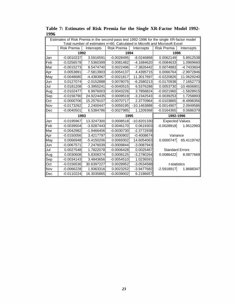
Table 7: Estimates of Risk Premia for the Single XR-Factor Model 1992-1996

Estimates of Risk Premia in the second-pass test 1992-1996 for the single XR-factor model Total number of estimates n=60, Calculated in Microfit and Microsoft Excel

Risk Premia Intercepts Risk Premia Intercepts Risk Premia Intercepts 1992 1994 1996 Jan -0.0010237 3.5916591 -0.0028495 -8.0246868 0.0062149 5.8912538Feb -0.0256578 7.5360399 0.0081482 -4.1684620 -0.0084633 1.0969660Mar -0.0015273 8.5474740 0.0022496 -7.3826442 0.0074883 -4.7433604Apr 0.0053891 -7.5813903 -0.0054137 4.4395715 0.0066764 -2.9972846May -0.0048680 -4.4383967 -0.0021817 11.3017697 -0.0220826 11.0629240Jun 0.0127074 -2.0152888 0.0078075 -6.2580213 -0.0170938 7.1652773Jul 0.0181208 -3.3955241 -0.0040515 6.5376288 0.0053730 -10.4606801Aug -0.0102477 6.9976003 -0.0043226 3.7858824 -0.0021960 -1.5828915Sep -0.0156790 24.9224435 0.0009519 -3.2342543 -0.0039253 1.7258893Oct -0.0000706 15.2579107 -0.0070717 2.3770964 -0.0103865 -8.4998356Nov -0.0173262 2.2400447 0.0059195 -10.1463888 -0.0014907 2.0949586Dec -0.0040501 6.5384786 -0.0027985 1.1209368 -0.0164365 0.0686379 1993 1995 1992-1996 Jan -0.0195967 13.3247300 0.0008518 -10.8201330 Expected Values Feb -0.0039504 -3.9287443 0.0046170 0.0619303 -0.0028918 1.9512993Mar -0.0042982 -1.9466406 -0.0030730 -2.3772938 Apr -0.0150056 3.4217797 0.0000902 -0.4008674 Variance May 0.0066948 -5.4150206 0.0069302 14.6054063 0.0000747 65.4119742Jun -0.0067571 7.2476039 -0.0009844 -3.0087943Jul 0.0027548 1.7822078 -0.0006428 0.0025467 Standard Errors Aug 0.0030608 5.8308374 0.0008125 -3.2780264 0.0086422 8.0877669Sep -0.0034143 3.4843656 -0.0054510 1.0236591Oct -0.0156536 30.6397227 0.0028952 -3.0534588 t-statistics Nov -0.0066228 1.9363316 0.0023252 -3.9477682 -2.5918917 1.8688347Dec -0.0110224 16.3035865 -0.0039002 6.2186657

24

References 1. Akrasanee, Narongchai, Jansen, Karel and Pongpisanupichit, Jeerasak. 1993.

International Capital Flows and Economic Adjustment in Thailand. Bangkok: The Thailand Development Research Institute.

2. Boadway, Robin, Flatters, Frank and Wen, Jean-Francois. 1992. Thailand Economic Structure: Towards Balanced Development? Required Returns on Investment by Small and Large Firms in Thailand: Case of Capital Differentials and the Fiscal Environment. Queen's University, Kingston, Canada.

3. Brown, Stephen J. and Weinstein, Mark I. 1983. "A New Approach to Testing Asset Pricing Models: The Bilinear Paradigm." The Journal of Finance, Vol. XXXVIII, No. 3, June 1983, pp. 711-743.

4. Chan, Louis K. C., Hamao Yasushi, and Lakonishok, Josef. 1991. "Fundamentals and Stock Returns in Japan." The Journal of Finance, Vol. XLVI, No. 5, December 1991, pp. 1739-1763.

5. Chen, Nai-Fu, Roll, Richard and Ross, Stephen A. 1986. "Economic Forces and the Stock Market." Journal of Business, Vol. 59, No. 3, 1986, pp. 383-403.

6. Chen, Nai-Fu. 1983. "Some Empirical Tests of the Theory of Arbitrage Pricing." The Journal of Finance, vol. XXXVIII, No. 5, December 1983, pp. 1393-1414.

7. Cho, D. Chinhyung, Elton, Edwin J. and Gruber, Martin J. 1984. "On the Robustness of the Roll and Ross Arbitrage Pricing Theory." Journal of Financial and Quantitative Analysis, Vol. 19, No. 1, March 1984, pp. 1-10.

8. Copeland, Thomas E. and Weston, J. Fred, Adapted by Fox, A.F. and Limmack, R.J. 1988. Managerial Finance. Second UK Edition. An Adaptation of Managerial Finance, Eighth Edition: 1986, New York: CBS College Publishing. Cassell Educational Limited, Reprinted 1995.

9. Copeland, Thomas E. and Weston, J. Fred. 1992. Financial Theory and Corporate Policy. Third Edition. Addison-Wesley Publishing Company, Inc., 1988, Reprinted with Corrections, May 1992.

10. Elton, Edwin J. and Gruber, Martin J. 1995. Modern Portfolio Theory and Investment Analysis. Fifth Edition. John Wiley & Sons, Inc.

11. Elton, Edwin, Gruber, Martin and Rentzler, Joel. 1983. "The Arbitrage Pricing Model and Returns on Assets Under Uncertain Inflation." The Journal of Finance, Vol. XXXVIII, No. 2, May 1983, pp. 525-537.

12. FactBook. 1996. The Thailand Stock Exchange, Thailand, 1996. 13. Fama, Eugene F. and MacBeth James D. 1973. "Risk, Return, and Equilibrium:

Empirical Tests." Journal of Political Economy, No. 38, 1973, pp. 607-636. 14. Fama, Eugene. 1970. "Effficient Capital Markets: A Review of Theory and

Empirical Work." Journal of Finance, XXV, No. 2, March 1970, pp. 383-417. 15. Greene, William H. 1993. Econometric Analysis. Second Edition. Prentice Hall

International Editions. 16. Gujarati, Damodar N. 1995. Basic Econometrics. Third Edition. McGraw-Hill,

Inc.: International Edition.

25

17. Jansen, Karel. 1987. Finance, Growth and Stability: Financing Economic Development in Thailand, 1960-1984. Vrije Universiteit te Amsterdam.

18. Kennedy, Peter. 1992. A Guide to Econometrics. Third Edition. Oxford UK & Cambridge USA: Blackwell.

19. Kitchen, Richard L. 1986. Finance for The Developing Countries. John Wiley & Sons, Inc.

20. Lintner, John. 1965. "The Valuation of Risk Assets and the Selection of Risky Investments in Stock Portfolios and Capital Budgets." Review of Economics and Statistics, No. 47, February 1965, pp. 13-37.

21. Maddala, G. S. 1988. Introduction to Econometrics. New York: Macmillan Publishing Company.

22. Mossin, Jan. 1966. "Equilibrium in a Capital Asset Market." Econometrica, No. 34, October 1966, pp. 768-783.

23. Osei, Kofi A. 1997. Asset Pricing and Information Efficiency of the Ghana Stock Market - A Final Research Report Submitted to AERC. School of Administration. University of Ghana. Offprint, December 1997.

24. Price, Margaret M. 1994. Emerging Stock Markets. A Complete Investment Guide to New Markets Around the World. McGraw-Hill, Inc.

25. Roll, Richard and Ross, Stephen A. 1980." An Empirical Investigation of the Arbitrage Pricing Theory." The Journal of Finance, Vol. XXXV, No. 5, December 1980, pp. 1073-1103.

26. Ross, Stephen A. 1976. "The Arbitrage Theory of Capital Asset Pricing." Journal of Economic Theory, Vol. 13, December 1976, pp. 341-360.

27. Setting Up in Thailand: A Guide for Investors. 1988. BLC Publishing Co., Ltd. 28. Sithi-Amnuai, Paul. 1964. Finance and Banking in Thailand: A study of the

commercial system, 1988-1963. Thailand: Thai Watana Panich. 29. Smith, Graham, Dinwiddy, Caroline and Hesselman, Linda. 1997. Econometric

Analysis and Applications. Offprint, SOAS, University of London. 30. Smith, Graham. 1997. Econometric Principles and Data Analysis. Offprint, SOAS,

University of London. 31. SETCP. 1994. Stock Exchange of Thailand Company Profiles. Dokbia Publishing

House. 32. Vichyanond, Pakorn. 1994. Thailand's Financial System: Structure and

Liberalization. Thailand: The Thailand Development Research Institute.