Arbitrage Asymmetry and the Idiosyncratic Volatility Puzzle

Arbitrage Asymmetry and the IdiosyncraticVolatility Puzzle

by*

Robert F. Stambaugh, Jianfeng Yu, and Yu Yuan

First Draft: October 1, 2012This Draft: January 9, 2013

Abstract

Short selling, as compared to purchasing, faces greater risks and other potentialimpediments. This arbitrage asymmetry explains the negative relation between id-iosyncratic volatility (IVOL) and average return. The IVOL effect is negative amongoverpriced stocks but positive among underpriced stocks, with mispricing determinedby combining 11 return anomalies. The negative effect is stronger, consistent withasymmetry in risks and other impediments inhibiting arbitrageurs in exploiting mis-pricing. Aggregating across all stocks therefore yields a negative relation, explainingthe IVOL puzzle. Further supporting our explanation is a negative relation over timebetween the IVOL effect and investor sentiment, especially among overpriced stocks.

* We are grateful for helpful comments from Lubos Pastor and seminar participants at the Shanghai

Advanced Institute of Finance, the University of Minnesota, University of Oxford, University of Toronto, and

the Wharton School. We also thank Edmund Lee and Jianan Liu for excellent research assistance. Author

affiliations/contact information:

Stambaugh: Miller, Anderson & Sherrerd Professor of Finance, The Wharton School, University of Penn-

sylvania and NBER, phone 215-898-5734, email [email protected].

Yu: Assistant Professor of Finance, The Carlson School of Management, University of Minnesota, phone

612-625-5498, email [email protected].

Yuan: Assistant Professor of Finance, Shanghai Advanced Institute of Finance, Shanghai Jiao Tong Uni-

versity, and Fellow, Wharton Financial Institutions Center, University of Pennsylvania, phone +86-21-6293-

2114, email [email protected].

1. Introduction

Does a stock’s expected return depend on “idiosyncratic” volatility that does not arise from

systematic risk factors? This question has been investigated empirically since virtually the

inception of classical asset pricing theory. Earlier empirical investigations often find no

relation, consistent with classical theory, or they find a positive relation between expected

return and idiosyncratic volatility (IVOL). Much of the recent empirical literature on this

topic, beginning notably with Ang, Hodrick, Xing, and Zhang (2006), instead finds a negative

relation between expected return and IVOL.1 While a positive relation is accommodated

by various theoretical departures from the classical paradigm, the negative relation has

presented more of a puzzle.2

This study presents an explanation for the observed negative relation between IVOL and

expected return. We start with the proposition that IVOL creates arbitrage risk that deters

market participants from exploiting mispricing and thereby correcting prices.3 We then

combine this familiar concept with what we term arbitrage asymmetry—the observation

that potential short sellers wishing to exploit overpricing face impediments to arbitrage

more than do potential purchasers wishing to exploit underpricing.4

Combining the effects of arbitrage risk and arbitrage asymmetry implies the observed

negative relation between IVOL and expected return. To see this, first note that stocks with

greater IVOL, and thus greater arbitrage risk, are more susceptible to mispricing. Among

overpriced stocks, the IVOL effect in expected return is therefore negative—those with the

highest IVOL are the most overpriced. Similarly, among underpriced stocks, the IVOL effect

is positive, as the highest IVOL stocks are then the most underpriced. With arbitrage asym-

1Recent studies finding a negative relation include Ang, Hodrick, Xing, and Zhang (2006, 2009), Jiang,Xu, and Yao (2009), Guo and Savickas (2010), and Chen, Jiang, Xu, and Yao (2012). The classic studyfinding no relation between expected return and IVOL is Fama and MacBeth (1973), who acknowledge themethodological issues raised by Miller and Scholes (1972) in their reexamination of Douglas (1968). A morerecent study finding no relation is Bali and Cakici (2008). Studies finding a positive relation include Lintner(1965), Tinic and West (1986), Lehmann (1990), Malkiel and Xu (2002), and Fu (2009).

2Explanations for a positive relation include Merton (1987), Barberis and Huang (2001), Malkiel and Xu(2002), and Jones and Rhodes-Kropf (2003).

3Studies addressing the role of arbitrage risk in mispricing include DeLong, Shleifer, Summers, andWaldmann (1990), Pontiff (1996), Shleifer and Vishny (1997), Mitchell, Pulvino, and Stafford (2002), andWurgler and Zhuravskaya (2002).

4Studies addressing the role of short-sale constraints and costs in the equity market include Miller (1977),Figlewski (1981), Chen, Hong, and Stein (2002), Diether, Malloy, and Scherbina (2002), Duffie, Garleanuand Pedersen (2002), Jones and Lamont (2002), D’Avolio (2002), Scheinkman and Xiong (2003), Lamont(2004), Lamont and Stein (2004), Ofek, Richardson, and Whitelaw (2004), Nagel (2005), Avramov, Chordia,Jostova, and Philipov (2012), and Stambaugh, Yu, and Yuan (2012a).

1

metry, however, more of the potential underpricing has been eliminated, thereby reducing

the differences in the degree of underpricing associated with different levels of IVOL. As a

result, the negative IVOL effect among overpriced stocks is stronger than the positive IVOL

effect among underpriced stocks. When aggregating across all stocks, the negative IVOL

effect therefore dominates and creates the observed IVOL puzzle.

We argue that a principal source of arbitrage asymmetry is risk. Short sellers are exposed

to short-run price fluctuations requiring additional capital contributions more than are pur-

chasers of stock. This observation (novel, to our knowledge) applies in particular to what

is often termed “noise-trader” risk (e.g., Shleifer and Vishny, 1997)—the risk that adverse

price moves necessitate closing a position before the eventual correction of mispricing would

yield a profit. Also, the inherent skewness in compounded returns contributes to greater

tail risk for short sellers over holding periods likely to be relevant to professional investment

managers.

Adding to the risk-related sources of arbitrage asymmetry are other impediments to

short selling that have been previously discussed in the literature. The sizes of institutions

engaged in shorting, such as hedge funds, are rather small in aggregate compared to the

sizes of mutual funds and other institutions that do not short. Hong and Sraer (2012) place

primary emphasis on this disparity in arguing that short sale impediments are important.5

D’Avolio (2002) finds that shorting costs, while generally low, increase in the dispersion of

opinion about a stock, consistent with a setting in which shorting becomes more expensive

precisely when less optimistic investors would wish to short a stock whose price is driven up

by the more optimistic investors.6

Our explanation of the IVOL puzzle is supported by the data. A key element of our em-

pirical work is constructing a proxy for mispricing. For this purpose, we average each stock’s

rankings associated with 11 return anomalies that survive adjustment for the three factors of

Fama and French (1993). Sorting stocks based on this composite anomaly ranking allows us

to investigate the IVOL effect within various degrees of relative mispricing. As predicted by

arbitrage risk combined with arbitrage asymmetry, the IVOL effect is significantly negative

(positive) among the most overpriced (underpriced) stocks, and the negative effect among

the overpriced stocks is significantly stronger.

5In making this point, the authors cite the low use of actual shorting by mutual funds, often due toinvestment policy restrictions, as documented by Almazan, Brown, Carlson, and Chapman (2004), as wellas mutual funds’ low use of derivatives, as documented by Koski and Pontiff (1999).

6Lamont (2004) discusses various impediments to short selling, and he also argues that impediments canbecome more severe precisely when a stock becomes more overpriced, sometimes due to action by a firm todeter shorting of its stock.

2

Additional implications of our explanation emerge when considering variation through

time in the likely market-wide direction of mispricing. Periods when overpricing is its

strongest are also those when we should observe the strongest negative IVOL effect among

stocks classified as relatively overpriced by the cross-sectional anomaly ranking. Similarly,

periods when underpricing is its strongest are those when we should observe the strongest

positive IVOL effect among stocks classified as relatively underpriced. With arbitrage asym-

metry, this variation in IVOL effects through time should be stronger for the stocks that are

relatively overpriced. Compared with low sentiment periods, during high sentiment periods

the negative IVOL effect among overpriced stocks is stronger, whereas the positive IVOL

effect among the underpriced stocks is weaker. Thus, when aggregating across all stocks, the

average negative relation between IVOL and expected return observed by previous studies

should be stronger in periods when there is a market-wide tendency for overpricing.

To identify periods when a given mispricing direction is more likely, we use the index

of market-wide investor sentiment constructed by Baker and Wurgler (2006).7 Consistent

with the above predictions, the negative IVOL effect among overpriced stocks is significantly

stronger following months when investor sentiment is high, and the positive IVOL effect

among underpriced stocks is significantly stronger following months when investor senti-

ment is low. These inferences are further supported by finding that a time series regression

of an IVOL return spread (high minus low) on investor sentiment produces a significantly

negative coefficient for both the overpriced and underpriced stocks. Arbitrage asymmetry

implies that this variation over time in IVOL effects should be stronger among the over-

priced stocks. Consistent with this prediction, the time-series regression reveals significantly

stronger sentiment-related variation in the IVOL effect among the overpriced stocks. When

aggregating across stocks, the overall negative IVOL effect on expected return should be

stronger following high sentiment, and this prediction is also confirmed in our results.

We focus here on explaining the relation between IVOL and expected return, but there

are additional empirical implications of our setting. In particular, among high-IVOL stocks,

mispricing, especially overpricing, should be stronger than among low-IVOL stocks. These

implications are in fact supported by Jin (2012), who finds that long-short spreads based

on a wide range of anomalies are more profitable among high-IVOL stocks, and this effect

7Related studies that investigate the role of investor sentiment in cross-sectional returns include Bakerand Wurgler (2006, 2007), Lemmon and Portniaguina (2006), Bergman and Roychowdhury (2008), Kaniel,Saar, and Titman (2008), Frazzini and Lamont (2008), Livnat and Petrovic (2008), Antoniou, Doukas, andSubrahmanyam (2012), Baker, Wurgler, and Yuan (2012), Chung, Hung, and Yeh (2012), Shen and Yu(2012), and Stambaugh, Yu, and Yuan (2012a, 2012b).

3

is especially strong for the short-leg profits.8 In another related study, Cao and Han (2010)

explore the role of IVOL-related arbitrage risk in mispricing. Those authors also sort stocks

based on a composite of anomaly rankings, and they also find a significantly negative (posi-

tive) IVOL effect among the relatively overpriced (underpriced) stocks. Their results do not

display a substantial asymmetry in the strength of those IVOL effects, nor do they discuss

asymmetry or the IVOL puzzle.9 Our hypothesized role of arbitrage asymmetry in the IVOL

effect is consistent with the event-study results of Doran, Jiang, and Peterson (2012), who

conclude that high-IVOL stocks experience negative returns after short-sale constraints are

relaxed.

Alternative explanations of the IVOL puzzle appear in a number of studies. Jiang, Xu,

and Yao (2009) argue that high IVOL is associated with firms that disclose less and that the

market does not correctly assess the negative valuation implication associated with selec-

tive low disclosure. Boehme, Danielson, Kumar, and Sorescu (2009) find that the negative

IVOL effect flips to positive when firms with high institutional ownership and high shorting

activity are eliminated. Boyer, Mitton, and Vorkink (2010) conclude that a negative rela-

tion between expected return and idiosyncratic skewness is at least a partial explanation for

the IVOL puzzle. Bali, Cakici, and Whitelaw (2011) argue that the IVOL puzzle reflects a

preference for lottery-like payoffs, captured better by maximum past return than by IVOL.

Huang, Liu, Rhee, and Zhang (2010) conclude that IVOL proxies for a return-reversal effect.

Barinov (2011) and Chen and Petkova (2012) conclude that IVOL proxies for sensitivity to a

priced volatility factor. While these alternative explanations may all be at work, they seem

challenged to reconcile the joint set of empirical results we present here: (i) the sign of the

IVOL effect depends on whether stocks are identified as overpriced or underpriced, (ii) the

negative (positive) IVOL effect among overpriced (underpriced) stocks is stronger following

high (low) investor sentiment, and (iii) both of the previous results are stronger among the

overpriced stocks.

The remainder of the paper is organized as follows. Section 2 describes our measure of

relative cross-sectional mispricing, based on a composite ranking that combines 11 return

8Other studies find greater long-short anomaly returns among high-IVOL stocks but do not document thestronger contribution that the short-leg (overpriced) stocks make to such results. E.g., Mendenhall (2002),Ali, Hwang, and Trombley (2003), Mashruwala, Rajgopal, and Shevlin (2006), Pontiff (2006), Zhang (2006),Cao and Han (2010), Duan, Hu, and McLean (2010), McLean (2010), Lam and Wei (2011), Li and Sullivan(2011), and Larrain and Varas (2012).

9A potential reason that asymmetry does not emerge as a feature of their study is that their anomalyranking measure could contain less information about mispricing, in that it combines only four anomalies,instead of our eleven, and two of those four are size and book-to-market, for which a mispricing interpretationmust contend with a significant literature arguing that those variables instead proxy for risk.

4

anomalies. Section 3 discusses arbitrage asymmetry, focusing in particular on asymmetry

in various risks faced by arbitrageurs. Section 4 presents our basic results showing that

the IVOL effect is positive among underpriced stocks but more strongly negative among

overpriced stocks. Section 5 explores the time-series implications of our setting, using investor

sentiment as a proxy for the likely direction of market-wide tendencies toward overpricing

or underpricing. Section 6 reviews the study’s main conclusions.

2. Identifying Mispricing

In our setting, mispricing is essentially the difference between the observed price and the price

that would otherwise prevail in the absence of arbitrage risk and other arbitrage impediments.

Of course, mispricing is not directly observable, and the best we can do is to construct an

imperfect proxy for it. An obvious resource for this purpose is the evidence on return

anomalies, which are differences in average returns that challenge risk-based models. We

first describe our approach to constructing a mispricing measure based on anomalies, and

we then detail our 11 return anomalies taken from the literature.

2.1. Mispricing Measure

We combine the anomalies to produce a univariate monthly measure that correlates with

the degree of relative mispricing in the cross section of stocks. While each anomaly is itself

a mispricing measure, our objective in combining them is to produce a single measure that

diversifies away some noise in each individual anomaly and thereby increases precision when

exploring the empirical implications of our setting.

Our method for combining the anomalies is simple. For each anomaly, we assign a rank

to each stock that reflects the sorting on that given anomaly variable, where the highest

rank is assigned to the value of the anomaly variable associated with the lowest average

abnormal return, as reported in the literature. For example, one documented anomaly is

that high asset growth in the previous year is followed by low return (Cooper, Gulen, and

Schill, 2008). We therefore rank firms each month by asset growth, and those with the

highest growth receive the highest rank. The higher the rank, the greater the relative degree

of overpricing according to the given anomaly variable. A stock’s composite rank is then the

arithmetic average of its ranks for each of the 11 anomalies. Thus, we refer to the stocks

with the highest composite ranking as the most “overpriced” and to those with the lowest

5

ranking as the most “underpriced.” The mispricing measure is purely cross-sectional, so

it is important to note that these designations at best denote only relative mispricing. At

any given time, for example, a stock identified as the most underpriced might actually be

overpriced. The intent of the measure is simply that such stocks would then be the least

overpriced within the cross section. We return to this point later, when investigating the

role of investor sentiment over time.

Evidence that our mispricing measure is effective in diversifying some of the noise in

anomaly rankings can be found in the range of average returns produced by sorting on

our measure. For example, if each month we assign stocks to ten categories based on our

measure and then form a value-weighted portfolio for each decile, the following month’s

spread in benchmark-adjusted returns between the two extreme deciles averages 1.48% over

our sample period, 8/1965–1/2011. (The returns are adjusted for exposures to the three

equity benchmarks constructed by Fama and French, 1993: MKT, SMB, and HML.) In

comparison, if value-weighted decile portfolios are first formed for each individual anomaly

ranking, and then the returns on those portfolios are combined with equal weights across

the 11 anomalies, the corresponding spread between the extreme deciles is 0.87%. In other

words, averaging the anomaly rankings produces an extra 61 basis points per month as

compared to averaging the anomaly returns. (The t-statistic of the difference is 4.88.)

We also find in the above comparison that ranking on our mispricing measure creates

additional abnormal return primarily among the stocks classified as overpriced. For exam-

ple, of the 62-basis-point improvement in the long-short return spread reported above, 57

basis points come from the most overpriced portfolio—the short leg of the corresponding

arbitrage strategy—and only 4 basis points come from the most underpriced—the long leg.

This asymmetry in improvement in arbitrage profits is consistent with arbitrage asymmetry:

With the latter asymmetry, one expects overpricing to be greater than underpricing, so a

better identification of mispricing should yield greater improvement in arbitrage profits for

overpriced stocks than for underpriced stocks.

2.2. Anomalies

To our knowledge, these anomalies constitute a fairly comprehensive list of those that survive

adjustment for the three factors of Fama and French (1993). The same anomalies are used

by Stambaugh, Yu, and Yuan (2012a).

1 and 2: Financial Distress

6

Financial distress is often invoked to explain otherwise anomalous patterns in the cross-

section of stock returns. However, Campbell, Hilscher, and Szilagyi (2008) find that firms

with high failure probability have lower rather than higher subsequent returns (anomaly 1).

Campbell et al. suggest that their finding is a challenge to standard models of rational asset

pricing. The failure probability is estimated by a dynamic logit model with both accounting

and equity market variables as explanatory variables. Using Ohlson’s (1980) O-score as the

distress measure yields similar results (anomaly 2). Ohlson’s (1980) O-score is calculated

as the probability of bankruptcy in a static model using accounting variables, such as net

income divided by assets, working capital divided by market assets, current liability divided

by current assets, and etc. The failure probability is different with the O-score in that it is

estimated by a dynamic, rather than a static model, and that the model uses several equity

market variables, such as stock prices, book-to-market, stock volatility, relative size to the

S&P 500, and cumulative excess return relative to S&P 500.

3 and 4: Net Stock Issues and Composite Equity Issues

The stock issuing market has been long viewed as producing an anomaly arising from

sentiment-driven mispricing: smart managers issue shares when sentiment-driven traders

push prices to overvalued levels. Ritter (1991) and Loughran and Ritter (1995) show that,

in post-issue years, equity issuers underperform matching nonissuers with similar character-

istics (anomaly 3). We measure net stock issues as the growth rate of the split-adjusted

shares outstanding in the previous fiscal year. Daniel and Titman (2006) study an alterna-

tive measure, composite equity issuance, defined as the amount of equity a firm issues (or

retires) in exchange for cash or services. Under this measure, seasoned issues and share-based

acquisitions increase the issuance measure, while repurchases, dividends and other actions

that take cash out of the firm reduce this issuance measure. They also find that issuers

underperform nonissuers (anomaly 4).

5: Total Accruals

Sloan (1996) shows that firms with high accruals earn abnormal lower returns on average

than firms with low accruals, and suggests that investors overestimate the persistence of

the accrual component of earnings when forming earnings expectations. Here, total accruals

are calculated as changes in non-cash working capital minus depreciation expense scaled by

average total assets for previous two fiscal years.

6: Net Operating Assets

7

Hirshleifer, Hou, Teoh, and Zhang (2004) find that net operating assets, defined as the

difference on the balance sheet between all operating assets and all operating liabilities scaled

by total assets, is a strong negative predictor of long-run stock returns. They suggest that

investors with limited attention tend to focus on accounting profitability, neglecting infor-

mation about cash profitability, in which case net operating assets, equivalently measured

as the cumulative difference between operating income and free cash flow, captures such a

bias.

7: Momentum

The momentum effect, discovered by Jegadeesh and Titman (1993), is one of the most

robust anomalies in asset pricing. It refers to the phenomenon that high past recent recent

returns forecast high future returns. The momentum portfolios we use are ranked based on

cumulative returns from month -7 to month -2, and the holding period for these portfolios

is 6-month. That is, it is a 6/1/6 momentum strategy.

8: Gross Profitability Premium

Novy-Marx (2012a) discovers that sorting on gross-profit-to-assets creates abnormal benchmark-

adjusted returns, with more profitable firms having higher returns than less profitable ones.

Novy-Marx (2012a) argues that gross profits (item GP) scaled by assets (item AT) are the

cleanest accounting measure of true economic profitability. The farther down the income

statement one goes, the more polluted profitability measures become, and the less related

they are to true economic profitability.

9: Asset Growth

Cooper, Gulen, and Schill (2008) find companies that grow their total asset more earn

lower subsequent returns. They suggest that this phenomenon is due to investors’ initial

overreaction to changes in future business prospects implied by asset expansions. Asset

growth is measured as the growth rate of the total assets (item AT) in the previous fiscal

year.

10: Return on Assets

Fama and French (2006) find that more profitable firms have higher expected returns than

less profitable firms. Chen, Novy-Marx, and Zhang (2010) show that firms with higher past

return-on-assets earn abnormally higher subsequent returns. Return-on-assets measured as

the ratio of the quarterly earnings (item IBQ) and last quarter’s assets (item ATQ). Wang

8

and Yu (2010) find that the anomaly exists primarily among firms with high arbitrage costs

and high information uncertainty, suggesting that mispricing is a culprit.

11: Investment-to-Assets

Titman, Wei, and Xie (2004) and Xing (2008) show that higher past investment predicts

abnormally lower future returns. Titman, Wei, and Xie (2004) attribute this anomaly to

investors’ initial underreactions to the overinvestment caused by managers’ empire-building

behavior. Here, investment-to-assets are measured as the annual change in gross property,

plant, and equipment plus the annual change in inventories scaled by the lagged book value

of assets.

3. Arbitrage Risk and Asymmetry

Arbitrageurs face various risks. One source of risk, often termed “noise-trader” risk (e.g.,

Shleifer and Vishny, 1997), is that adverse price moves can require additional capital in

order to maintain positions that involve shorting or leverage. As a result, capital constraints

can necessitate closing positions before realizing profits that would ultimately result from

corrections of mispricing. Another source of risk is simply new information. An arbitrageur

can purchase a stock today that he correctly identifies as underpriced based on available

information, but negative information about the stock’s fundamental value can later be

revealed and cause a loss. Investment managers often care about performance over relatively

short periods such as a year. Sufficiently bad performance over such periods, whether from

noise traders or new information, could cost a manager his job, or at least reduce the capital

that investors allow him to manage.

Our setting combines two simple concepts. First, greater arbitrage risk allows greater

mispricing, as such risk deters arbitrageurs from exploiting mispricing and thereby correct-

ing it. Second, arbitrage impediments are asymmetric, inhibiting short selling of overpriced

stocks more than they inhibit purchasing of underpriced stocks. Combining these two con-

cepts yields the implication that a given difference in arbitrage risk is associated with a

greater average degree of overpricing as compared to underpricing.

The above implication follows generally, whatever the source of asymmetry in arbitrage

impediments. As discussed earlier, previously noted potential sources of asymmetric imped-

iments include restrictions against short selling faced by many institutions, such as mutual

funds, as well as occasionally high shorting costs. A key source of asymmetric impediments,

9

although perhaps one less recognized, is arbitrage risk itself. In the first subsection below,

we discuss why short sellers face greater arbitrage risk than purchasers.

If arbitrageurs can neutralize their exposure to benchmark risks, a seemingly reasonable

assumption, then idiosyncratic volatility (IVOL), as opposed to total volatility, is more

closely related to arbitrage risk. Moreover, arbitrageurs can hold positions in multiple stocks

at a given time, thereby enjoying diversification benefits. Therefore, the IVOL of the return

on a portfolio of stocks that are overpriced more directly translates to arbitrage risk for a

short seller, as compared to the IVOL’s of the individual stocks. Similarly, the IVOL of a

portfolio of underpriced stocks translates more directly to arbitrage risk for a purchaser.10 In

the second subsection below, we examine the idiosyncratic volatilities of returns on portfolios

formed within various levels of our mispricing measure.

3.1. Asymmetric Arbitrage Risk

The risks faced by arbitrageurs are likely to be greater for short sellers than for purchasers.

Consider first the risk that additional capital will be required to maintain a position. As

noted above, this is a feature of noise-trader risk. In general, shorting requires that a margin

deposit be maintained at some percentage of position size. If the price of the shorted stock

rises, increasing the position size, additional margin capital can be required. A purchaser

who does not employ leverage does not face margin calls, so in that case the greater risk

facing the short seller is obvious.

A short seller still faces greater risk of a margin call even compared to a purchaser who

buys on margin. To see this, note first that a position’s margin ratio, which must typically

be maintained above a specified maintenance level, is computed as

m =equity

position size. (1)

Now consider a short seller and a purchaser, identical in terms of both equity and position

sizes, who subsequently experience identical adverse rates of return on their underlying

securities. Given the identical absolute return magnitudes, the short seller and purchaser

lose identical amounts of equity, so they still have identical values for the numerator in

(1). The new denominators differ from each other, however. The position size decreases

10One might note that the underlying issue is essentially the manner and extent to which correlationsamong benchmark-adjusted returns enter portfolio volatilities. If the benchmark-adjusted returns are id-iosyncratic in the strongest sense—uncorrelated with each other across all stocks—the individual-stock IVOLremains the relevant quantity. See Pontiff (2006) for a discussion of this point.

10

for the purchaser but increases for the short seller, so the short seller’s m declines by a

greater amount. This asymmetry leaves short sellers more exposed to margin calls. For

example, if both the long and short positions are established with m = 50%, and they both

have maintenance requirements of m = 25%, the purchaser receives a margin call if the

security price drops by 33%, whereas the short seller receives a call if the price increases

by 20%. In practice, this asymmetry is magnified by stricter maintenance requirements for

short positions. For example, the Financial Industry Regulatory Authority (FINRA), which

regulates U.S. brokerage firms, specifies m = 25% for long positions but m = 30% for short

positions.11 With the latter requirement, the above short seller receives a margin call if the

price increases by only 15.4%, less than half the percentage move triggering a call on the

long position.

The risk of a large loss over an evaluation period such as a year can also be greater for

the short seller simply because of the skewness inherent to compounded returns. Suppose a

short seller and purchaser initially start with equal position sizes. If each of them experiences

the same adverse percentage change in value of their underlying securities in the first month,

their dollar losses are the same in that month. If that month is followed by another month of

identical adverse percentage changes in security values, the short seller’s total two-month loss

then exceeds that of the purchaser. The reason is that, after the first month, the purchaser’s

position size decreases while the short seller’s position increases. In essence, the compounding

effect positively skews multiperiod returns, and the positive skewness translates to greater

tail risk for a short seller. To better see the potential effect of such tail risk, suppose a short

seller and a purchaser take equal sized positions in underlying portfolios each having monthly

returns that are lognormal with a standard deviation of 4%. The short seller’s underlying

portfolio has an expected monthly return, after trading costs, equal to -0.50%, whereas

the purchaser’s portfolio has an expected return of 0.50%. Now consider the 1% Value-at-

Risk (VaR) over 12 months—the amount of 12-month dollar loss for which the probability

of a greater loss is equal to 1% (assuming both positions remain open). Straightforward

calculations reveal that the short seller’s VaR is 22% greater than the purchaser’s VaR.

Another source of asymmetry in arbitrage risk is that short positions can occasionally

be squeezed. As with the noise-trader risk mentioned earlier, this risk can necessitate the

premature closing of an eventually profitable position. Specifically, a lender can recall a

stock loan, at which point the short seller can find it difficult to locate a new lender.12 There

11See FINRA Rule 4210.12This risk is discussed, for example, by Dechow, Hutton, Meulbroek, and Sloan (2001), who cite circum-

stances surrounding the stock of Amazon.com in June 1998 as as a notable instance of a short squeeze.

11

is no corresponding risk for long positions.

3.2. Idiosyncratic Volatilities of Portfolios

This study provides an explanation of the previously reported negative relation between

average return and IVOL, where IVOL is computed at the individual-stock level (Ang,

Hodrick, Xing, and Zhang, 2006). As noted earlier, arbitrage risk, which is central to our

explanation, is more appropriately related to the idiosyncratic volatility of a portfolio than

to a single stock. Thus, an important step in our empirical investigation is to confirm that

differences among individual-stock IVOL’s translate to corresponding differences in portfolio

IVOL’s.

Table 1 reports idiosyncratic volatilities of portfolio returns sorted by mispricing and

individual-stock IVOL. We compute individual-stock IVOL following Ang, Hodrick, Xing,

and Zhang (2006), using the most recent month’s daily benchmark-adjusted returns.13 The

latter returns are computed as the residuals in a regression of each stock’s daily return on

the three factors defined by Fama and French (1993): MKT, SMB, and HML. Each month,

portfolios are formed by sorting first on the mispricing measure, forming five categories, and

then by sorting within each of those categories by individual-stock IVOL, again forming five

categories. At both stages, equal numbers of stocks are allocated to each category. The stocks

within each of the resulting 25 portfolios are value weighted to form the portfolio returns.

The portfolio IVOL’s reported in Table 1 are computed using the monthly portfolio returns,

adjusted by the Fama-French factors, over the sample period covering 8/1965–1/2011.

The results in Table 1 confirm that within each level of mispricing, portfolio IVOL obeys

the same ordering as the underlying individual-stock IVOL used in the sorting. For exam-

ple, within the category of the most overpriced securities, the highest-IVOL portfolio has a

monthly IVOL of 4.43%, and then IVOL’s decline monotonically to 2.49% for the lowest-

IVOL portfolio. Within the category of the most underpriced, we see portfolio IVOL’s decline

monotonically from 3.39% for the highest-IVOL portfolio to 1.82% for the lowest-IVOL port-

folio. Similar patterns occur in the other three mispricing categories. We can thus conclude

that diversification does not eliminate the differences in arbitrage risk that trace to different

levels of individual-stock IVOL.

13This method is common in recent studies, but there are alternative approaches, such as the EGARCHmodel in Fu (2009). Guo, Kassa, and Ferguson (2012), and Fink, Fink, and He (2012) argue that thepositive relation between expected return and IVOL found by Fu (2009) owes to the use of contemporaneousinformation in the conditional variance model and does not survive after controlling for such information.

12

Another result evident in Table 1 is that IVOL is higher among overpriced stocks than

among underpriced stocks. This asymmetry in IVOL’s is in fact consistent with our hypoth-

esized setting. If arbitrage risk is an important determinant of the degree of mispricing, then

the more mispriced securities will tend to have higher risk. With asymmetric impediments

to arbitrage, however, overpricing is more likely than underpricing. Sorting on a relative mis-

pricing measure is therefore likely to be more effective at the overpriced end in identifying

high-risk stocks. If the impediments to arbitrage were instead symmetric, one should expect

a U-shaped pattern in going from the top to the bottom of Table 1. With the asymmetry,

the U-shape gets weakened among the underpriced stocks in the bottom rows. As a result,

we see at best only the hint of a U-shape.

4. Mispricing and IVOL Effects

Table 2 presents the first set of our main results. The table reports average benchmark-

adjusted monthly returns for each of the same 25 double sorted portfolios in Table 1. We

see results consistent with the role of IVOL-driven arbitrage risk in mispricing. Among the

securities most likely to be mispriced, as identified by our mispricing measure, we expect

to see the magnitude of mispricing increase with IVOL. The patterns in average returns

are consistent with that prediction. For the most overpriced securities, the average re-

turns are negative and monotonically decreasing in IVOL, with the difference between the

highest- and lowest-IVOL portfolios equal to -1.80% per month (t-statistic: -8.28). For the

most underpriced securities, the average returns are positive and monotonically increasing in

IVOL, with the difference between the highest- and lowest-IVOL portfolios equal to 0.57%

per month (t-statistic: 3.30). For the stocks in the middle of the mispricing scale, there

is no apparent IVOL effect: there is no monotonicity, and the highest-versus-lowest differ-

ence is only -0.18% per month (t-statistic: -0.95). The role of mispricing in determining

the strength and direction of IVOL effects is readily apparent in Figure 1, which plots the

average benchmark-adjusted returns reported in Table 2.

Also evident in Table 2 and Figure 1 is the asymmetry in IVOL effects predicted by asym-

metry in arbitrage impediments. The negative IVOL effect among the overpriced stocks is

stronger than the positive IVOL effect among the underpriced stocks. The negative highest-

versus-lowest difference among the most overpriced stocks is 3.2 times the magnitude of the

corresponding positive difference among the most underpriced stocks. This asymmetry ex-

plains the negative IVOL effect obtained when aggregating across all stocks, as shown in the

13

last row of Table 2. Among all stocks, consistent with the IVOL puzzle, average return is

monotonically decreasing in IVOL, with the highest-versus-lowest difference equal to -0.78%

per month (t-statistic: -5.50).

An additional implication of our setting is that the degree of mispricing, especially over-

pricing, should be greater among high-IVOL stocks than among low-IVOL stocks. We see

this implication supported as well. The difference in average portfolio returns between the

most overpriced stocks and the most underpriced stocks is negative and decreasing in IVOL,

as shown in the next to last row in Table 2. The difference between that short-long differ-

ence for the highest-IVOL portfolios versus the lowest-IVOL portfolios is -2.38% per month

(t-statistic: -9.08). These results are consistent with those of Jin (2012), who finds that

that long-short spreads on each of ten anomalies are more profitable among high-IVOL

stocks than among low-IVOL stocks, and that this difference in profitability is attributable

primarily to the short legs of each strategy.

Recall that Table 2 is constructed by first sorting stocks into five categories based on the

mispricing measure and then, within each mispricing quintile, sorting stocks into five cate-

gories based on IVOL. This dependent two-way sort allows us to focus on how IVOL effects

depend on the direction and degree of mispricing. At the same time, however, the dependent

sort potentially sacrifices some clarity in understanding how these IVOL effects aggregate

across stocks to deliver the overall negative IVOL relation, since the breakpoints for IVOL

differ across mispricing quintiles. As a robustness check, we also do an independent two-way

sort, so that each of the mispricing-IVOL combinations simply contains the intersection of

separate one-way sorts on mispricing and IVOL. The same 5 × 5 array reported in Table 2 is

reported in Table 3, but with the independent sort replacing the dependent sort. As before,

we see a significantly positive monthly return difference between high-IVOL and low-IVOL

stocks among the most underpriced stocks (0.41 percent, t-statistic: 2.16), and we see a

stronger negative IVOL effect among the most overpriced stocks (-1.50 percent, t-statistic:

-7.36). Since the IVOL breakpoints are the same across the mispricing quintiles in Table 3,

it is easier to see how the IVOL effects within those quintiles aggregate to deliver the overall

negative IVOL effect reported in the last row of Table 2.14

14As an additional robustness check, we also recompute Table 2 using equally weighted portfolios ratherthan value-weighted portfolios, and the results are very similar: (i) a positive IVOL effect among the mostunderpriced (0.37 percent, t-statistic: 3.19), (ii) a stronger negative IVOL effect among the most overpriced(-1.73 percent, t-statistic: -10.66), and (iii) a negative overall IVOL effect (-0.83 percent, t-statistic: -7.33).

14

5. Time-Varying IVOL Effects

In our setting, the IVOL effects in expected return hinge on mispricing. If the degree

and direction of mispricing vary over time, so should the IVOL effects. To investigate

such time-varying IVOL effects, we need to identify variation over time in the tendency for

general overpricing or underpricing in the stock market. For this purpose, we rely on the

index of market-wide investor sentiment constructed by Baker and Wurgler (2006). The

Baker-Wurgler (BW) index is constructed as the first principal component of six underlying

measures of investor sentiment: the average closed-end fund discount, the number and the

first-day returns of IPO’s, NYSE turnover, the equity share of total new issues, and the

dividend premium (log difference of average market/book of dividend payers vs. nonpayers).

The first subsection below investigates whether IVOL effects vary over time with investor

sentiment in a manner predicted by our explanation. The results indicate that they do. For

this initial investigation of sentiment effects, we use the “raw” version of the BW index

from which macroeconomic effects are not removed. The reason for doing so is that investor

sentiment could be related to macroeconomic factors. For example, when the economy is

doing well, investors could also be more optimistic, and thus more likely to push prices above

fundamental values. While such macro-related sentiment effects are perfectly consistent

with our setting, many readers might ask whether they play a role in our results. In the

second subsection below, we investigate this question by using Baker and Wurgler’s (2006)

alternative sentiment measure, which removes the effects of six macro variables. We further

include six additional macro variables that previous empirical studies relate to expected

stock returns. Our results point to little or no role for macro factors in the sentiment-related

variation in the IVOL effects that we observe.

5.1. Investor Sentiment and IVOL Effects

Recall that our mispricing measure at best identifies only relative mispricing. Periods of

high investor sentiment, when overpricing in the stock market is more likely in general, are

also those times when our relatively overpriced stocks are more likely to be overpriced in

absolute terms. At such times, the negative IVOL effect among our “overpriced” stocks

should be stronger than at other times. That is, the IVOL effect (highest minus lowest)

should be negatively related to the level of investor sentiment among the overpriced stocks.

Similarly, in periods of low investor sentiment, our relatively underpriced stocks are more

likely to be underpriced in absolute terms. At those times, the positive IVOL effect among

15

our “underpriced” stocks should be stronger than otherwise. In other words, among the

underpriced stocks as well, the IVOL effect (highest minus lowest) should be negatively

related to the level of investor sentiment. Therefore, among both overpriced and underpriced

stocks, the IVOL effect should be negatively related to investor sentiment. As a result, the

overall negative IVOL effect observed when aggregating across stocks should be stronger

following high sentiment.

To explore the above implications, Table 4 repeats the analysis in Table 2 separately for

high-sentiment and low-sentiment months. The three intermediate categories of IVOL are

omitted to save space in Table 4. Figure 2 displays the averages for all five IVOL categories

in low-sentiment and high-sentiment months. A high-sentiment month is one in which the

value of the BW sentiment index at the end of the previous month is above the median

value for the 1965:8–2011:1 sample period, while the low-sentiment months are those with

below-median index values in the previous month.

The results in Table 4 and Figure 2 support the implications of our setting. First ob-

serve that among all stocks (bottom row), the negative IVOL effect is significantly stronger

following high sentiment, as predicted. The spread between the highest-IVOL and lowest-

IVOL average returns is -1.32% following high sentiment compared to -0.23% following low

sentiment—a difference of -1.09% (t-statistic: -3.82). Also as predicted, the relatively over-

priced stocks exhibit this same pattern. Among the most overpriced stocks, the spread

between the highest-IVOL and lowest-IVOL average returns is -2.30% following high senti-

ment compared to -1.30% following low sentiment—a difference of -1.00% (t-statistic: -2.29).

For the most underpriced stocks, the positive IVOL effect is stronger following low sentiment

than following high sentiment: Among those stocks, the spread between the highest-IVOL

and lowest-IVOL average returns is 0.21% following high sentiment compared to 0.94% fol-

lowing low sentiment—a difference of -0.73% (t-statistic: -2.03). These results go in the

direction of supporting arbitrage asymmetry as well, in that the sentiment-related difference

in IVOL effects is somewhat larger for the most overpriced stocks, although the t-statistic

for the difference is modest (-0.53). When interpreting this last result, one should probably

consider that a binary split between high- and low-sentiment periods, while useful in its

simplicity, does not necessarily yield the most powerful test. We next turn to time-series

regression as an alternative approach.

Table 5 reports the results of regressing excess returns or return spreads in month t

on the variable St−1, the level of the BW index at the end of the previous month. Also

included as independent variables are the contemporaneous realizations of the Fama-French

16

factors (MKT, SMB, and HML), so the slope on St−1 reflects sentiment-related variation in

the benchmark-adjusted returns. The dependent variable in the regressions is either (i) the

(excess) return on the highest-IVOL portfolio, (ii) the return on the lowest-IVOL portfolio, or

(iii) the difference between those returns. These three regressions are run separately within

each mispricing category and within the overall stock universe.

The results in Table 5 are again supportive of our setting’s implications. Consistent with

Table 4, the IVOL effect (highest minus lowest IVOL) is negatively related to investor sen-

timent. Within the overall stock universe, the slope on St−1 is equal to -0.66 (t-statistic:

-4.25), meaning that a one-standard-deviation swing in St−1 is associated with a 66-basis-

point difference in the IVOL effect. In addition, that negative slope is largest in magnitude

among the most overpriced stocks, and the difference between the slopes for the most over-

priced versus the most underpriced stocks is equal to -0.50 (t-statistic: -2.20).

Our use of the BW index as an independent variable in time-series regressions follows, for

example, Baker and Wurgler (2006) and Stambaugh, Yu, and Yuan (2012a). One potential

concern in any time-series regression is that a seemingly significant relation is spurious.

This concern looms larger, the weaker is the prior motivation for the independent variable.

Investor sentiment has long been entertained as exerting a significant influence on stock prices

(e.g., Keynes, 1936), but spurious-regressor concerns can nevertheless arise. Indeed such a

concern with regard to investor sentiment is raised by Novy-Marx (2012b). Simulations

reported by Stambaugh, Yu and Yuan (2012b) reveal that the spurious regressor concern

is greatly diminished when considering the ability of such a regressor to generate predicted

results across a number of regressions.

5.2. Exploring macroeconomic effects

As mentioned earlier, investor sentiment could be related to macroeconomic factors. It is

quite possible, for example, that when macroeconomic conditions are especially good, some

investors also become too optimistic and push equity prices above levels justified by funda-

mental values. Similarly, during recessions, some investors could become too pessimistic and

undervalue stocks as a result. As long as high (low) sentiment makes overpricing (under-

pricing) more likely, the extent to which sentiment relates to the macroeconomy does not

affect the implications explored above. Nevertheless, the extent to which macroeconomic

conditions play a role in our results are of potential interest.

Baker and Wurgler (2006) construct an alternative sentiment index that removes macro-

17

related variation by regressing their raw sentiment measures on six macro variables: the

growth in industrial production, the growth in durable, nondurable, and services consump-

tion, the growth in employment, and a flag for NBER recessions. Panel A of Table 6 repeats

the regressions in Table 5 using this alternative sentiment index. The results are very similar

to those in Table 5, indicating no important role for the six Baker-Wurgler macro variables

in the former results. In Panel B of Table 5, we repeat the regression in Panel A but add six

additional macro-related independent variables: the default premium, the term premium,

the real interest rate, the inflation rate, the consumption surplus ratio, and CAY. These

variables are often identified as being related to expected stock returns, so they seem es-

pecially relevant for exploring the role of macroeconomic conditions in our results. The

default premium is defined as the yield spread between BAA and AAA bonds, and the term

premium is defined as the spread between 20-year and 1-year Treasuries. The real interest

rate is defined as the most recent monthly difference between the 30-day T-bill return and

the CPI inflation rate. The consumption surplus ratio defined in Campbell and Cochrane

(1999). Cay is the consumption-wealth variable defined in Lettau and Ludvigson (2001).15

The conclusions summarized previously based on Table 5 are again essentially unchanged if

instead based Panel B of Table 6. Overall, the results in Table 6 indicate that the sentiment-

related variation in IVOL effects admit little or no role for the macro variables included in

our investigation.

We do not include macro variables directly related to the stock market, such as dividend

yield. In this sense, our choice of macro variables differs from that of Sibley, Xing, and Zhang

(2012). Those authors investigate whether it is macro-related sentiment or non-macro-related

sentiment that displays the ability to predict anomaly returns, as documented in Stambaugh,

Yu, and Yuan (2012a). Sibley, Xing, and Zhang conclude that it is largely macro-related

sentiment that exhibits the predictive ability. Such a result is consistent with sentiment-

driven mispricing in any event, but the distinction between macro and non-macro effects

seems less interesting when the macro variables include stock-market variables. Sentiment

that affects stock prices is likely to affect dividend yield, lowering yield when sentiment is

high, and vice versa. One would expect a sentiment measure purged of those stock-price

effects to be less effective in identifying sentiment-driven stock mispricing and, therefore, to

be less effective in predicting anomaly returns that reflect such mispricing.16

15The bond yields are obtained from the St. Louis Federal Reserve, the T-bill return and inflation areobtained from CRSP, and Cay is obtained from Sydney Ludvigson’s website. Following Wachter (2006), thesurplus ratio is calculated as a smoothed average of past consumption growth.

16Additional stock-market variables included by Sibley, Xing, and Zhang (2012) are volatility and a liq-uidity measure. Liquidity in particular could contain sentiment effects. In fact, Baker and Wurgler (2006)include turnover as one of the variables constituting their sentiment index.

18

6. Excluding Smaller Firms

In this section we explore the sensitivity of our results to excluding smaller firms. It is well

known that smaller firms tend to have higher IVOL, and we also find that firm size tends to

decline as our mispricing measure increases (i.e., as the measure moves from underpriced to

overpriced). The fact that size is related to both IVOL and our mispricing measure raises

the question of whether our results hinge importantly on including small firms. Our use of

value-weighted portfolios in the previous results reduces this possibility, but in this section

we go further and explore the sensitivity of our results to excluding firms below a given size

threshold.

Table 7 repeats the analysis reported earlier in Table 2 but with smaller firms excluded.

Before performing the two-way sort on IVOL and the mispricing measure, we eliminate all

firms whose equity capitalization falls in the bottom p percent of the stock universe, for

various choices of p. Specifically, in Panels A, B, C, and D, of Table 7, we exclude the

bottom 20 percent, 40 percent, 60 percent, and 80 percent, respectively. First observe from

Table 2 and Table 7 that the overall negative relation between IVOL and average return

progressively weakens as the size threshold increases, but even among the largest quintile

of stocks (Panel D) the average monthly spread between the high- and low-IVOL portfolios

is still -0.37 percent (t-statistic: -2.59). This result is consistent with the results in Ang,

Hodrick, Xing, and Zhang (2006), who find that the IVOL puzzle exists within all size

quintiles but is weaker for larger firms.

The key result for the purpose of this study is that, as the size threshold increases,

the IVOL effect continues to display the same dependence on the direction and degree of

mispricing as observed earlier in Table 2. That is, the IVOL effect is significantly nega-

tive (positive) among the most overpriced (underpriced) stocks, but the negative effect is

significantly stronger. We do observe that the latter asymmetry weakens somewhat as the

size threshold increases, which is consistent with the corresponding weakening of the overall

IVOL effect. Even for the largest stocks (Panel D), however, the negative IVOL effect among

the most overpriced stocks (-0.88 percent, t-statistic: -4.09) exceeds the positive IVOL effect

among the most underpriced stocks (0.48 percent, t-statistic: 2.62) by a difference of -1.35

percent (t-statistic: -5.32).

We do observe that the weakening of the asymmetry as the threshold increases comes

primarily from the weakening of the negative IVOL effect among the overpriced stocks. For

the portfolio of the most overpriced stocks, the IVOL effect starting in Table 2 and then

19

progressing through the four panels of Table 7 takes the values -1.80, -1.69, -1.58, -1.25, and

-0.88, which display a clear increasing pattern. Among the most underpriced stocks, the

comparable values are 0.57, 0.58, 0.63, 0.60, and 0.48, which display little or no pattern. In

other words, as progressively larger stocks are eliminated, the positive IVOL effect among

the most underpriced stocks remains fairly stable in magnitude, whereas the negative IVOL

effect among the most overpriced stocks weakens.

Finally, we repeat the analysis in Table 5 under the same progressive elimination of

smaller firms employed in Table 7, and the results are reported in Table 8. In all four panels

of Table 8, the IVOL effect among overpriced stocks exhibits a significantly negative relation

to investor sentiment, with magnitudes ranging from -0.79 to -0.91, comparable to the value

of -0.79 in Table 5. The IVOL effect among underpriced stocks exhibits a consistently weaker

negative relation to sentiment, again as in Table 5. We do see that excluding smaller firms

causes the t-statistics for those negative coefficients to drop below conventional significance

levels. Finding a weaker negative relation among the underpriced stocks is consistent with

arbitrage asymmetry, as discussed earlier.

7. Conclusions

We provide an explanation for the negative empirical relation between expected return and

idiosyncratic volatility (IVOL) observed in the overall cross section of equities. Our expla-

nation combines two simple concepts. The first is that higher IVOL, which translates to

higher arbitrage risk, allows greater mispricing. As a result, expected return is negatively

(positively) related to IVOL among overpriced (underpriced) securities. The second con-

cept is that arbitrage is asymmetric, in that short sellers face greater impediments than

purchasers. Combining these two concepts yields the implication that a given difference in

IVOL is associated with a greater average degree of overpricing as compared to underpricing.

That is, the negative IVOL effect among overpriced securities is stronger than the positive

effect among underpriced, and thus a negative IVOL effect emerges within the overall cross

section.

Our empirical evidence supports our explanation. First, using a composite measure based

on 11 return anomalies to gauge relative mispricing, we find a significant positive IVOL

effect among the most underpriced stocks but a stronger negative effect among the most

overpriced ones, consistent with arbitrage asymmetry. We also empirically confirm time-

series implications of our explanation. Using investor sentiment as a proxy for the likely

20

direction of market-wide mispricing, we find that the negative (positive) IVOL effect among

overpriced (underpriced) stocks is stronger when market-wide overpricing (underpricing) is

more likely. This negative relation over time between investor sentiment and the return

difference between high- and low-volatility portfolios is stronger among overpriced stocks,

consistent with the presence of arbitrage asymmetry.

We argue that risk is a key source of arbitrage asymmetry. One source of risk that

is greater for short sellers is having to close prematurely an eventually profitable position

due to adverse price moves—often termed noise-trader risk. The risk of a short squeeze

necessitating a premature closure also has no long-side counterpart. Short sellers also face

tail risk to a greater degree, due to the positive skewness in returns over periods likely to be

relevant for professional investment managers.

21

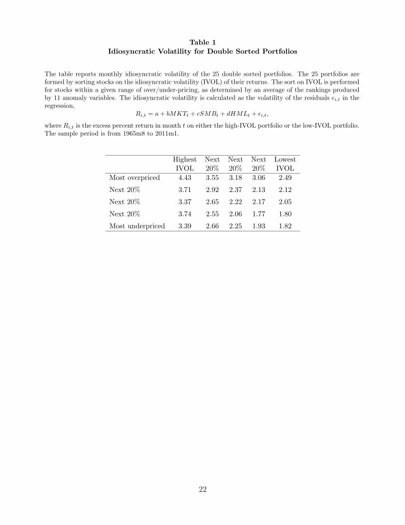
Table 1Idiosyncratic Volatility for Double Sorted Portfolios

The table reports monthly idiosyncratic volatility of the 25 double sorted portfolios. The 25 portfolios areformed by sorting stocks on the idiosyncratic volatility (IVOL) of their returns. The sort on IVOL is performedfor stocks within a given range of over/under-pricing, as determined by an average of the rankings producedby 11 anomaly variables. The idiosyncratic volatility is calculated as the volatility of the residuals ϵi,t in theregression,

Ri,t = a+ bMKTt + cSMBt + dHMLt + ϵi,t,

where Ri,t is the excess percent return in month t on either the high-IVOL portfolio or the low-IVOL portfolio.The sample period is from 1965m8 to 2011m1.

Highest Next Next Next LowestIVOL 20% 20% 20% IVOL

Most overpriced 4.43 3.55 3.18 3.06 2.49

Next 20% 3.71 2.92 2.37 2.13 2.12

Next 20% 3.37 2.65 2.22 2.17 2.05

Next 20% 3.74 2.55 2.06 1.77 1.80

Most underpriced 3.39 2.66 2.25 1.93 1.82

22

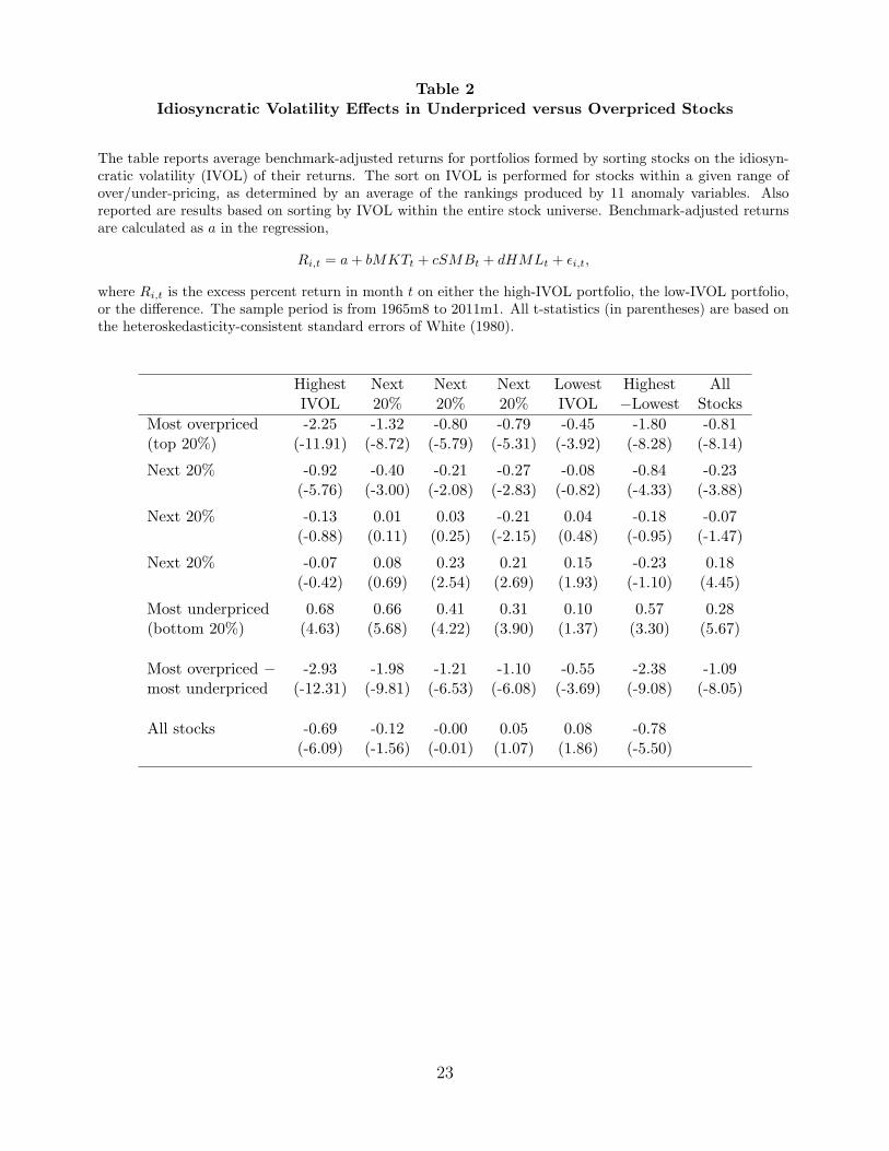
Table 2Idiosyncratic Volatility Effects in Underpriced versus Overpriced Stocks

The table reports average benchmark-adjusted returns for portfolios formed by sorting stocks on the idiosyn-cratic volatility (IVOL) of their returns. The sort on IVOL is performed for stocks within a given range ofover/under-pricing, as determined by an average of the rankings produced by 11 anomaly variables. Alsoreported are results based on sorting by IVOL within the entire stock universe. Benchmark-adjusted returnsare calculated as a in the regression,


where Ri,t is the excess percent return in month t on either the high-IVOL portfolio, the low-IVOL portfolio,or the difference. The sample period is from 1965m8 to 2011m1. All t-statistics (in parentheses) are based onthe heteroskedasticity-consistent standard errors of White (1980).

Highest Next Next Next Lowest Highest AllIVOL 20% 20% 20% IVOL −Lowest Stocks

Most overpriced -2.25 -1.32 -0.80 -0.79 -0.45 -1.80 -0.81(top 20%) (-11.91) (-8.72) (-5.79) (-5.31) (-3.92) (-8.28) (-8.14)

Next 20% -0.92 -0.40 -0.21 -0.27 -0.08 -0.84 -0.23(-5.76) (-3.00) (-2.08) (-2.83) (-0.82) (-4.33) (-3.88)

Next 20% -0.13 0.01 0.03 -0.21 0.04 -0.18 -0.07(-0.88) (0.11) (0.25) (-2.15) (0.48) (-0.95) (-1.47)

Next 20% -0.07 0.08 0.23 0.21 0.15 -0.23 0.18(-0.42) (0.69) (2.54) (2.69) (1.93) (-1.10) (4.45)

Most underpriced 0.68 0.66 0.41 0.31 0.10 0.57 0.28(bottom 20%) (4.63) (5.68) (4.22) (3.90) (1.37) (3.30) (5.67)

Most overpriced − -2.93 -1.98 -1.21 -1.10 -0.55 -2.38 -1.09most underpriced (-12.31) (-9.81) (-6.53) (-6.08) (-3.69) (-9.08) (-8.05)

All stocks -0.69 -0.12 -0.00 0.05 0.08 -0.78(-6.09) (-1.56) (-0.01) (1.07) (1.86) (-5.50)

23

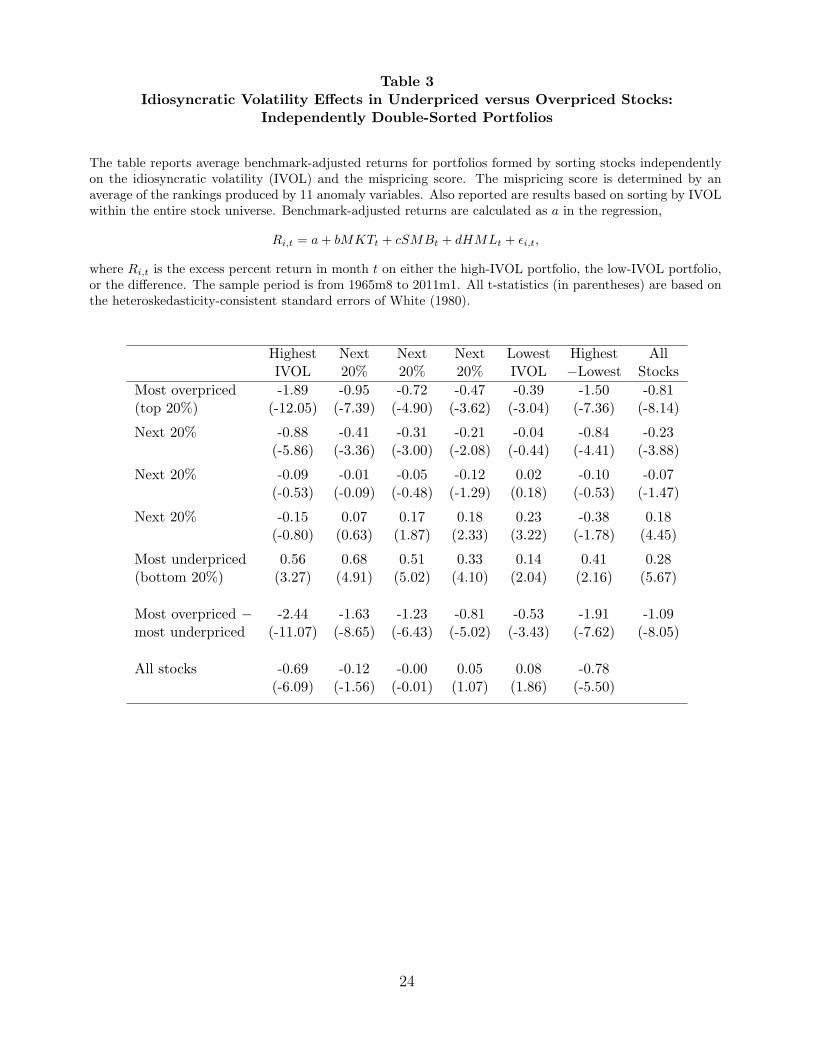
Table 3Idiosyncratic Volatility Effects in Underpriced versus Overpriced Stocks:

Independently Double-Sorted Portfolios

The table reports average benchmark-adjusted returns for portfolios formed by sorting stocks independentlyon the idiosyncratic volatility (IVOL) and the mispricing score. The mispricing score is determined by anaverage of the rankings produced by 11 anomaly variables. Also reported are results based on sorting by IVOLwithin the entire stock universe. Benchmark-adjusted returns are calculated as a in the regression,


where Ri,t is the excess percent return in month t on either the high-IVOL portfolio, the low-IVOL portfolio,or the difference. The sample period is from 1965m8 to 2011m1. All t-statistics (in parentheses) are based onthe heteroskedasticity-consistent standard errors of White (1980).



Next 20% -0.88 -0.41 -0.31 -0.21 -0.04 -0.84 -0.23(-5.86) (-3.36) (-3.00) (-2.08) (-0.44) (-4.41) (-3.88)

Next 20% -0.09 -0.01 -0.05 -0.12 0.02 -0.10 -0.07(-0.53) (-0.09) (-0.48) (-1.29) (0.18) (-0.53) (-1.47)

Next 20% -0.15 0.07 0.17 0.18 0.23 -0.38 0.18(-0.80) (0.63) (1.87) (2.33) (3.22) (-1.78) (4.45)


Most overpriced − -2.44 -1.63 -1.23 -0.81 -0.53 -1.91 -1.09most underpriced (-11.07) (-8.65) (-6.43) (-5.02) (-3.43) (-7.62) (-8.05)

All stocks -0.69 -0.12 -0.00 0.05 0.08 -0.78(-6.09) (-1.56) (-0.01) (1.07) (1.86) (-5.50)

24

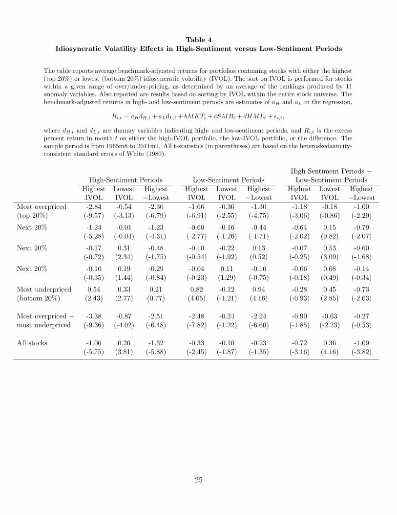
Table 4Idiosyncratic Volatility Effects in High-Sentiment versus Low-Sentiment Periods

The table reports average benchmark-adjusted returns for portfolios containing stocks with either the highest(top 20%) or lowest (bottom 20%) idiosyncratic volatility (IVOL). The sort on IVOL is performed for stockswithin a given range of over/under-pricing, as determined by an average of the rankings produced by 11anomaly variables. Also reported are results based on sorting by IVOL within the entire stock universe. Thebenchmark-adjusted returns in high- and low-sentiment periods are estimates of aH and aL in the regression,

Ri,t = aHdH,t + aLdL,t + bMKTt + cSMBt + dHMLt + ϵi,t,

where dH,t and dL,t are dummy variables indicating high- and low-sentiment periods, and Ri,t is the excesspercent return in month t on either the high-IVOL portfolio, the low-IVOL portfolio, or the difference. Thesample period is from 1965m8 to 2011m1. All t-statistics (in parentheses) are based on the heteroskedasticity-consistent standard errors of White (1980).

High-Sentiment Periods −High-Sentiment Periods Low-Sentiment Periods Low-Sentiment Periods

Highest Lowest Highest Highest Lowest Highest Highest Lowest HighestIVOL IVOL −Lowest IVOL IVOL −Lowest IVOL IVOL −Lowest

Most overpriced -2.84 -0.54 -2.30 -1.66 -0.36 -1.30 -1.18 -0.18 -1.00(top 20%) (-9.57) (-3.13) (-6.79) (-6.91) (-2.55) (-4.75) (-3.06) (-0.86) (-2.29)

Next 20% -1.24 -0.01 -1.23 -0.60 -0.16 -0.44 -0.64 0.15 -0.79(-5.28) (-0.04) (-4.31) (-2.77) (-1.26) (-1.71) (-2.02) (0.82) (-2.07)

Next 20% -0.17 0.31 -0.48 -0.10 -0.22 0.13 -0.07 0.53 -0.60(-0.72) (2.34) (-1.75) (-0.54) (-1.92) (0.52) (-0.25) (3.09) (-1.68)

Next 20% -0.10 0.19 -0.29 -0.04 0.11 -0.16 -0.06 0.08 -0.14(-0.35) (1.44) (-0.84) (-0.23) (1.29) (-0.75) (-0.18) (0.49) (-0.34)

Most underpriced 0.54 0.33 0.21 0.82 -0.12 0.94 -0.28 0.45 -0.73(bottom 20%) (2.43) (2.77) (0.77) (4.05) (-1.21) (4.16) (-0.93) (2.85) (-2.03)

Most overpriced − -3.38 -0.87 -2.51 -2.48 -0.24 -2.24 -0.90 -0.63 -0.27most underpriced (-9.36) (-4.02) (-6.48) (-7.82) (-1.22) (-6.60) (-1.85) (-2.23) (-0.53)

All stocks -1.06 0.26 -1.32 -0.33 -0.10 -0.23 -0.72 0.36 -1.09(-5.75) (3.81) (-5.88) (-2.45) (-1.87) (-1.35) (-3.16) (4.16) (-3.82)

25

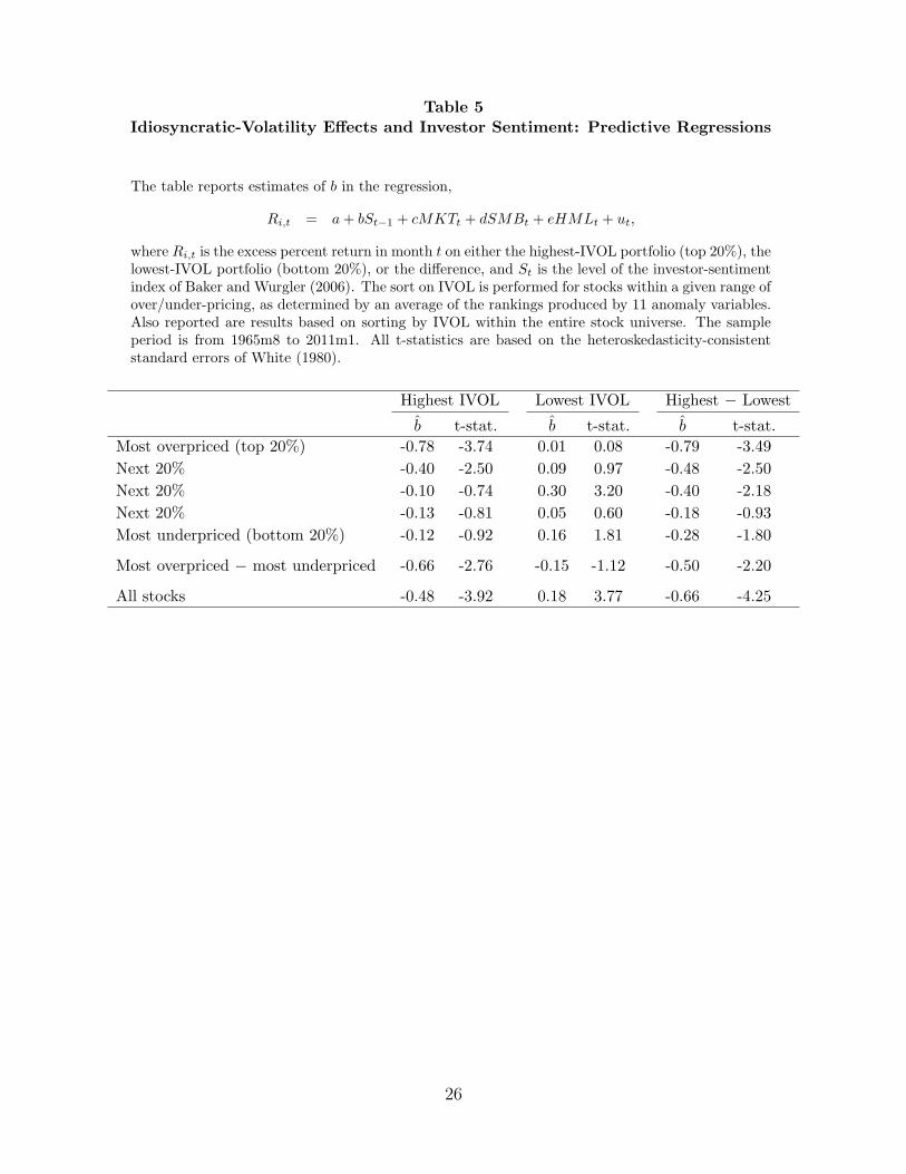
Table 5Idiosyncratic-Volatility Effects and Investor Sentiment: Predictive Regressions

The table reports estimates of b in the regression,

Ri,t = a+ bSt−1 + cMKTt + dSMBt + eHMLt + ut,

where Ri,t is the excess percent return in month t on either the highest-IVOL portfolio (top 20%), thelowest-IVOL portfolio (bottom 20%), or the difference, and St is the level of the investor-sentimentindex of Baker and Wurgler (2006). The sort on IVOL is performed for stocks within a given range ofover/under-pricing, as determined by an average of the rankings produced by 11 anomaly variables.Also reported are results based on sorting by IVOL within the entire stock universe. The sampleperiod is from 1965m8 to 2011m1. All t-statistics are based on the heteroskedasticity-consistentstandard errors of White (1980).

Highest IVOL Lowest IVOL Highest − Lowest

b t-stat. b t-stat. b t-stat.

Most overpriced (top 20%) -0.78 -3.74 0.01 0.08 -0.79 -3.49

Next 20% -0.40 -2.50 0.09 0.97 -0.48 -2.50

Next 20% -0.10 -0.74 0.30 3.20 -0.40 -2.18

Next 20% -0.13 -0.81 0.05 0.60 -0.18 -0.93

Most underpriced (bottom 20%) -0.12 -0.92 0.16 1.81 -0.28 -1.80

Most overpriced − most underpriced -0.66 -2.76 -0.15 -1.12 -0.50 -2.20

All stocks -0.48 -3.92 0.18 3.77 -0.66 -4.25

26

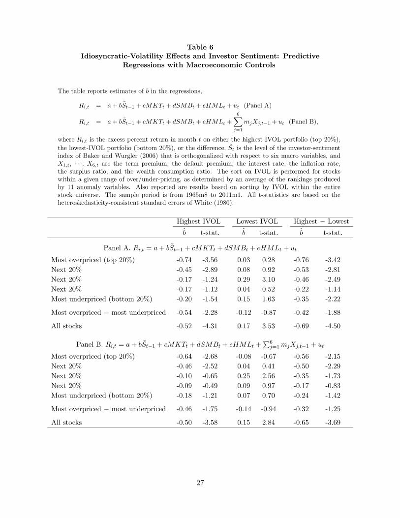
Table 6Idiosyncratic-Volatility Effects and Investor Sentiment: Predictive

Regressions with Macroeconomic Controls

The table reports estimates of b in the regressions,

Ri,t = a+ bSt−1 + cMKTt + dSMBt + eHMLt + ut (Panel A)

Ri,t = a+ bSt−1 + cMKTt + dSMBt + eHMLt +6∑

j=1

mjXj,t−1 + ut (Panel B),

where Ri,t is the excess percent return in month t on either the highest-IVOL portfolio (top 20%),

the lowest-IVOL portfolio (bottom 20%), or the difference, St is the level of the investor-sentimentindex of Baker and Wurgler (2006) that is orthogonalized with respect to six macro variables, andX1,t, · · ·, X6,t are the term premium, the default premium, the interest rate, the inflation rate,the surplus ratio, and the wealth consumption ratio. The sort on IVOL is performed for stockswithin a given range of over/under-pricing, as determined by an average of the rankings producedby 11 anomaly variables. Also reported are results based on sorting by IVOL within the entirestock universe. The sample period is from 1965m8 to 2011m1. All t-statistics are based on theheteroskedasticity-consistent standard errors of White (1980).



Panel A. Ri,t = a+ bSt−1 + cMKTt + dSMBt + eHMLt + ut

Most overpriced (top 20%) -0.74 -3.56 0.03 0.28 -0.76 -3.42

Next 20% -0.45 -2.89 0.08 0.92 -0.53 -2.81

Next 20% -0.17 -1.24 0.29 3.10 -0.46 -2.49

Next 20% -0.17 -1.12 0.04 0.52 -0.22 -1.14



All stocks -0.52 -4.31 0.17 3.53 -0.69 -4.50

Panel B. Ri,t = a+ bSt−1 + cMKTt + dSMBt + eHMLt +∑6

j=1mjXj,t−1 + ut

Most overpriced (top 20%) -0.64 -2.68 -0.08 -0.67 -0.56 -2.15

Next 20% -0.46 -2.52 0.04 0.41 -0.50 -2.29

Next 20% -0.10 -0.65 0.25 2.56 -0.35 -1.73

Next 20% -0.09 -0.49 0.09 0.97 -0.17 -0.83



All stocks -0.50 -3.58 0.15 2.84 -0.65 -3.69

27

Table 7Idiosyncratic Volatility Effects in Underpriced versus Overpriced Stocks

Under Various Thresholds for Market Capitalization



where Ri,t is the excess percent return in month t on either the high-IVOL portfolio, the low-IVOL portfolio,or the difference. The sample period is from 1965m8 to 2011m1. All t-statistics (in parentheses) are basedon the heteroskedasticity-consistent standard errors of White (1980). In Panels A, B, C, and D, the smallest20%, 40%, 60%, and 80% of the firms are deleted from the portfolio formation, respectively.


Panel A: 20% Smallest Stocks Deleted


Next 20% -0.89 -0.40 -0.25 -0.30 -0.10 -0.79 -0.26(-5.72) (-2.92) (-2.51) (-3.12) (-1.03) (-4.16) (-4.33)

Next 20% -0.13 0.07 0.05 -0.15 0.04 -0.17 -0.05(-0.89) (0.67) (0.49) (-1.55) (0.46) (-0.93) (-1.15)

Next 20% -0.04 0.11 0.21 0.22 0.13 -0.17 0.16(-0.22) (1.06) (2.25) (2.72) (1.68) (-0.87) (4.06)


Most overpriced − -2.83 -1.96 -1.23 -1.05 -0.56 -2.27 -1.09Most underpriced (-11.46) (-9.80) (-6.67) (-5.72) (-3.70) (-8.43) (-7.98)

All stocks -0.69 -0.05 0.03 0.02 0.09 -0.78(-6.13) (-0.69) (0.46) (0.51) (2.02) (-5.56)

Panel B: 40% Smallest Stocks Deleted


Next 20% -0.85 -0.33 -0.36 -0.27 -0.05 -0.81 -0.25(-5.61) (-2.57) (-3.38) (-2.86) (-0.46) (-4.21) (-4.17)

Next 20% -0.01 0.07 0.06 -0.15 0.04 -0.05 -0.03(-0.10) (0.67) (0.56) (-1.61) (0.45) (-0.31) (-0.74)

Next 20% 0.01 0.13 0.17 0.25 0.14 -0.12 0.17(0.09) (1.22) (1.83) (3.14) (1.74) (-0.65) (4.02)



All stocks -0.63 -0.03 0.08 0.01 0.10 -0.73(-5.63) (-0.39) (1.46) (0.25) (2.19) (-5.20)

28

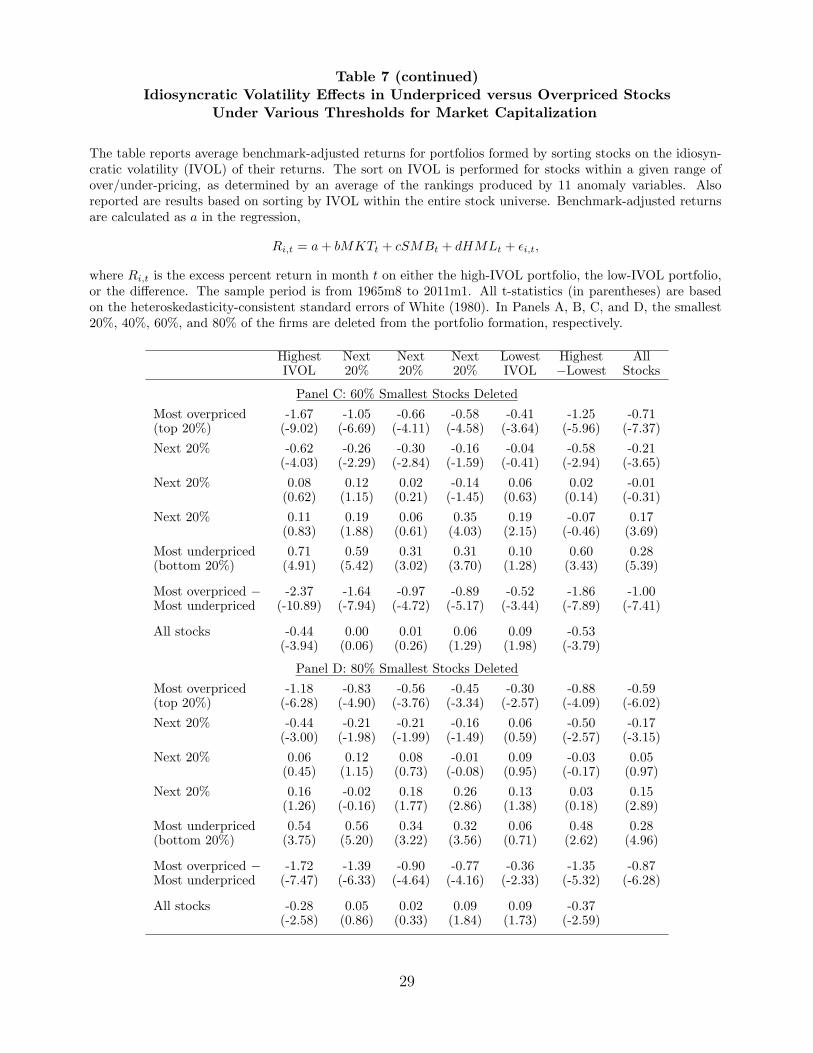
Table 7 (continued)Idiosyncratic Volatility Effects in Underpriced versus Overpriced Stocks




where Ri,t is the excess percent return in month t on either the high-IVOL portfolio, the low-IVOL portfolio,or the difference. The sample period is from 1965m8 to 2011m1. All t-statistics (in parentheses) are basedon the heteroskedasticity-consistent standard errors of White (1980). In Panels A, B, C, and D, the smallest20%, 40%, 60%, and 80% of the firms are deleted from the portfolio formation, respectively.


Panel C: 60% Smallest Stocks Deleted


Next 20% -0.62 -0.26 -0.30 -0.16 -0.04 -0.58 -0.21(-4.03) (-2.29) (-2.84) (-1.59) (-0.41) (-2.94) (-3.65)

Next 20% 0.08 0.12 0.02 -0.14 0.06 0.02 -0.01(0.62) (1.15) (0.21) (-1.45) (0.63) (0.14) (-0.31)

Next 20% 0.11 0.19 0.06 0.35 0.19 -0.07 0.17(0.83) (1.88) (0.61) (4.03) (2.15) (-0.46) (3.69)



All stocks -0.44 0.00 0.01 0.06 0.09 -0.53(-3.94) (0.06) (0.26) (1.29) (1.98) (-3.79)

Panel D: 80% Smallest Stocks Deleted


Next 20% -0.44 -0.21 -0.21 -0.16 0.06 -0.50 -0.17(-3.00) (-1.98) (-1.99) (-1.49) (0.59) (-2.57) (-3.15)

Next 20% 0.06 0.12 0.08 -0.01 0.09 -0.03 0.05(0.45) (1.15) (0.73) (-0.08) (0.95) (-0.17) (0.97)

Next 20% 0.16 -0.02 0.18 0.26 0.13 0.03 0.15(1.26) (-0.16) (1.77) (2.86) (1.38) (0.18) (2.89)



All stocks -0.28 0.05 0.02 0.09 0.09 -0.37(-2.58) (0.86) (0.33) (1.84) (1.73) (-2.59)

29

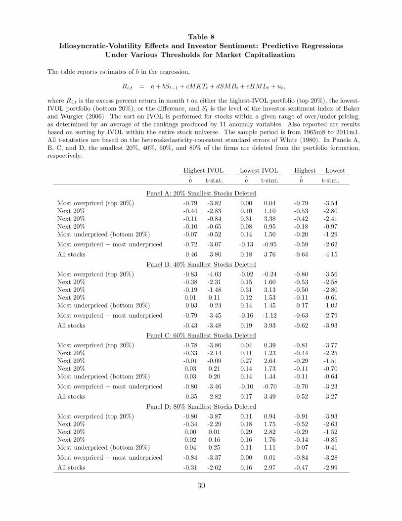
Table 8Idiosyncratic-Volatility Effects and Investor Sentiment: Predictive Regressions


The table reports estimates of b in the regression,

Ri,t = a+ bSt−1 + cMKTt + dSMBt + eHMLt + ut,

where Ri,t is the excess percent return in month t on either the highest-IVOL portfolio (top 20%), the lowest-IVOL portfolio (bottom 20%), or the difference, and St is the level of the investor-sentiment index of Bakerand Wurgler (2006). The sort on IVOL is performed for stocks within a given range of over/under-pricing,as determined by an average of the rankings produced by 11 anomaly variables. Also reported are resultsbased on sorting by IVOL within the entire stock universe. The sample period is from 1965m8 to 2011m1.All t-statistics are based on the heteroskedasticity-consistent standard errors of White (1980). In Panels A,B, C, and D, the smallest 20%, 40%, 60%, and 80% of the firms are deleted from the portfolio formation,respectively.



Panel A: 20% Smallest Stocks Deleted

Most overpriced (top 20%) -0.79 -3.82 0.00 0.04 -0.79 -3.54Next 20% -0.44 -2.83 0.10 1.10 -0.53 -2.80Next 20% -0.11 -0.84 0.31 3.38 -0.42 -2.41Next 20% -0.10 -0.65 0.08 0.95 -0.18 -0.97Most underpriced (bottom 20%) -0.07 -0.52 0.14 1.50 -0.20 -1.29


All stocks -0.46 -3.80 0.18 3.76 -0.64 -4.15

Panel B: 40% Smallest Stocks Deleted

Most overpriced (top 20%) -0.83 -4.03 -0.02 -0.24 -0.80 -3.56Next 20% -0.38 -2.31 0.15 1.60 -0.53 -2.58Next 20% -0.19 -1.48 0.31 3.13 -0.50 -2.80Next 20% 0.01 0.11 0.12 1.53 -0.11 -0.61Most underpriced (bottom 20%) -0.03 -0.24 0.14 1.45 -0.17 -1.02


All stocks -0.43 -3.48 0.19 3.93 -0.62 -3.93

Panel C: 60% Smallest Stocks Deleted

Most overpriced (top 20%) -0.78 -3.86 0.04 0.39 -0.81 -3.77Next 20% -0.33 -2.14 0.11 1.23 -0.44 -2.25Next 20% -0.01 -0.09 0.27 2.64 -0.29 -1.51Next 20% 0.03 0.21 0.14 1.73 -0.11 -0.70Most underpriced (bottom 20%) 0.03 0.20 0.14 1.44 -0.11 -0.64


All stocks -0.35 -2.82 0.17 3.49 -0.52 -3.27

Panel D: 80% Smallest Stocks Deleted

Most overpriced (top 20%) -0.80 -3.87 0.11 0.94 -0.91 -3.93Next 20% -0.34 -2.29 0.18 1.75 -0.52 -2.63Next 20% 0.00 0.01 0.29 2.82 -0.29 -1.52Next 20% 0.02 0.16 0.16 1.76 -0.14 -0.85Most underpriced (bottom 20%) 0.04 0.25 0.11 1.11 -0.07 -0.41

Most overpriced − most underpriced -0.84 -3.37 0.00 0.01 -0.84 -3.28

All stocks -0.31 -2.62 0.16 2.97 -0.47 -2.99

30

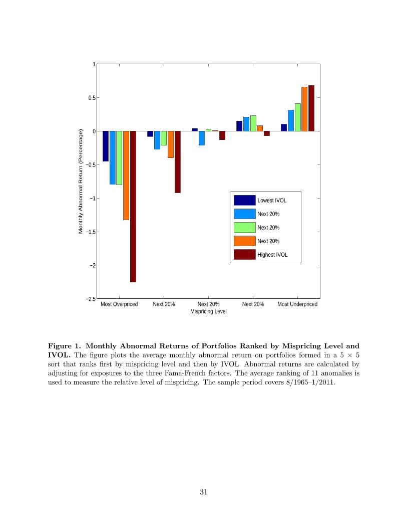
Most Overpriced Next 20% Next 20% Next 20% Most Underpriced−2.5

−2

−1.5

−1

−0.5

0

0.5

1

Mispricing Level

Mo

nth

ly A

bn

orm

al R

etu

rn (

Pe

rce

nta

ge

)

Lowest IVOL

Next 20%

Next 20%

Next 20%

Highest IVOL

Figure 1. Monthly Abnormal Returns of Portfolios Ranked by Mispricing Level andIVOL. The figure plots the average monthly abnormal return on portfolios formed in a 5 × 5sort that ranks first by mispricing level and then by IVOL. Abnormal returns are calculated byadjusting for exposures to the three Fama-French factors. The average ranking of 11 anomalies isused to measure the relative level of mispricing. The sample period covers 8/1965–1/2011.

31

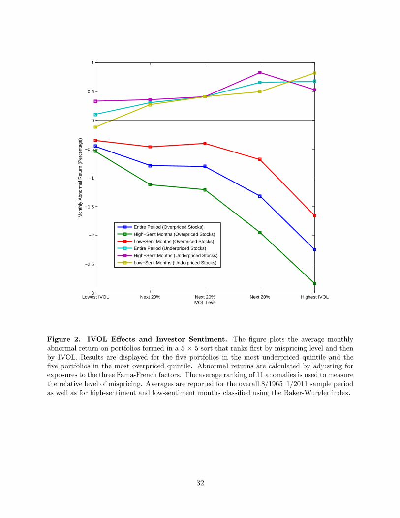
Lowest IVOL Next 20% Next 20% Next 20% Highest IVOL−3

−2.5

−2

−1.5

−1

−0.5

0

0.5

1

IVOL Level

Mon

thly

Abn

orm

al R

etur

n (P

erce

ntag

e)

Entire Period (Overpriced Stocks)

High−Sent Months (Overpriced Stocks)

Low−Sent Months (Overpriced Stocks)

Entire Period (Underpriced Stocks)

High−Sent Months (Underpriced Stocks)

Low−Sent Months (Underpriced Stocks)

Figure 2. IVOL Effects and Investor Sentiment. The figure plots the average monthlyabnormal return on portfolios formed in a 5 × 5 sort that ranks first by mispricing level and thenby IVOL. Results are displayed for the five portfolios in the most underpriced quintile and thefive portfolios in the most overpriced quintile. Abnormal returns are calculated by adjusting forexposures to the three Fama-French factors. The average ranking of 11 anomalies is used to measurethe relative level of mispricing. Averages are reported for the overall 8/1965–1/2011 sample periodas well as for high-sentiment and low-sentiment months classified using the Baker-Wurgler index.

32

References

Ali, A., Hwang, L., and Trombley, M.A., 2003, Arbitrage risk and the book-to-market anomaly,Journal of Financial Economics 69, 355–373.

Almazan, Andres, Keith C. Brown, Murray Carlson, and David A. Chapman, 2004, Why constrainyour mutual fund manager?, Journal of Financial Economics 73, 289–321.

Ang, A., R. Hodrick, Y. Xing, and X. Zhang, 2006, The cross-section of volatility and expectedreturns, Journal of Finance 51, 259–299.

Ang, A., R. Hodrick, Y. Xing, and X. Zhang, 2009, High idiosyncratic volatility and low returns:International and further U.S. evidence, Journal of Financial Economics 91, 1–23.

Antoniou, Constantinos, John A. Doukas, and Avanidhar Subrahmanyam, 2012, Sentiment andmomentum, Journal of Financial and Quantitative Analysis, forthcoming.

Avramov, Doron, Tarun Chordia, Gergana Jostova, and Alexander Philipov, 2012, Anomalies andfinancial distress, working paper, Hebrew University.

Baker, Malcolm, and Jeffrey Wurgler, 2006, Investor Sentiment and the Cross-section of StockReturns, Journal of Finance, 61, 1645–1680.

Baker, Malcolm, Wurgler, Jeffrey, 2007, Investor Sentiment in the Stock Market, Journal ofEconomic Perspectives 21, 129-152.

Baker, Malcolm, Jeffrey Wurgler, and Yu Yuan, 2012, Global, Local, and Contagious InvestorSentiment, Journal of Financial Economics 104, 272–287.

Bali, T., and N. Cakici ,2008, Idiosyncratic Volatility and the Cross-Section of Expected Re-turns,Journal of Financial and Quantitative Analysis 43, 29–58.

Bali, T., N. Cakici, and R. Whitelaw, 2011, Maxing out: Stocks as lotteries and the cross-sectionof expected returns, Journal of Financial Economics 99, 427–446.

Barberis, Nicholas and Ming Huang, 2001, Mental accounting, loss aversion, and individual stockreturns, Journal of Finance 56, 1247–1292.

Barinov, Alexander, 2011, Idiosyncratic Volatility, Growth Options, and the Cross-Section of Re-turns, working paper, University of Georgia.

Bergman, N. and S. Roychowdhury, 2008, Investor Sentiment and Corporate Disclosure, Journalof Accounting Research 46, 1057–1083.

Boehme, Rodney, Bartley Danielsen, Praveen Kumar, and Sorin Sorescu, 2009, Idiosyncratic riskand the cross-section of stock returns: Merton (1987) meets Miller (1977), Journal of FinancialMarkets 12, 438–468.

Boyer, B., T. Mitton, and K. Vorkink, 2010, Expected idiosyncratic skewness, Review of FinancialStudies 23, 169–202.

33

Campbell, John, and John Cochrane 1999, By force of habit: A consumption-based explanation ofaggregate stock market behavior, Journal of Political Economy 107, 205-251.

Campbell, John Y., Jens Hilscher, and Jan Szilagyi, 2008, In search of distress risk, Journal ofFinance 63, 2899–2939.

Carhart, Mark, 1997, On persistence in mutual fund performance, Journal of Finance 52, 57-82.

Cao, Jie, and Bing Han, 2010, Idiosyncratic Risk, Costly Arbitrage, and Cross-section of StockReturns, Working paper, The University of Texas at Austin.

Chen, Long, Robert Novy-Marx, and Lu Zhang, 2010, An alternative three-factor model, workingpaper, CKGSB, University of Rochester, and Ohio State University.

Chen, J., Hong, H., Stein, J.C., 2002. Breadth of ownership and stock returns. Journal of FinancialEconomics 66, 171–205.

Chen, Linda, George J. Jiang, Danielle Xu, and Tong Yao, 2012, Dissecting the IdiosyncraticVolatility Anomaly, working paper, Washington State University.

Chen, Zhanhui, and Ralitsa Petkova, 2012, Does Idiosyncratic Volatility Proxy for Risk Exposure?Review of Financial Studies, Forthcoming.

Chung, San-Lin, Chi-Hsiou Hung, and Chung-Ying Yeh, 2012, When does investor sentiment pre-dict stock returns?, Journal of Empirical Finance 19, 217–240.

Cooper, Michael J., Huseyin Gulen, and Michael J. Schill, 2008, Asset growth and the cross-sectionof stock returns, Journal of Finance 63, 1609–1652.

Daniel, Kent D., and Sheridan Titman, 2006, Market reactions to tangible and intangible informa-tion, Journal of Finance 61, 1605–1643.

Dechow, Patricia M., Amy P. Hutton, Lisa Meulbroek, and Richard G. Sloan, 2001, Short-sellers,fundamental analysis, and stock returns, Journal of Financial Economics 61, 77-106.

DeLong, Bradford, Andrei Shleifer, Lawrence H. Summers, and Robert Waldmann, 1990, Noisetrader risk in financial market. Journal of Political Economy, 90, 703–738.

Diether, K.B., Malloy, K.B., Scherbina, A., 2002. Differences of opinion and the cross-section ofstock returns. Journal of Finance 57, 2113-2141.

Doran, J., D. Jiang, and D. Peterson, 2012, Gambling in the New Year? The January idiosyncraticvolatility puzzle, Review of Finance, Forthcoming.

Douglas, George W., 1968, Risk in the Equity Markets: An Empirical Appraisal of Market Effi-ciency, University Microfilms Inc., Ann Arbor.

Duan, Y., Hu, G., and McLean, R.D., 2010 Costly arbitrage and idiosyncratic risk: evidence fromshort sellers, Journal of Financial Intermediation 19, 564–579.

Duffie, Darrell, Nicolae Garleanu, and Lasse Heje Pedersen, 2002, Securities lending shorting andpricing, Journal of Financial Economics 66, 307–339.

34

D’Avolio, G., 2002, The market for borrowing stock, Journal of Financial Economics 66, 271-306.

Fama, Eugene and Kenneth French, 1993, Common risk factors in the returns on stocks and bonds.Journal of Financial Economics 33, 3–56.

Fama, Eugene and Kenneth French, 2006, Profitability, investment, and average returns. Journalof Financial Economics 82, 491–518.

Fama, Eugene F. and James D. MacBeth, 1973, Risk, Return, and Equilibrium: Empirical Tests.The Journal of Political Economy 81, 607–636.

Figlewski, S., 1981, The informational effects of restrictions on short sales: some empirical evidence.Journal of Financial and Quantitative Analysis 16, 463–476.

Fink, J.; K. Fink; and H. He, 2012, Expected Idiosyncratic Volatility Measures and ExpectedReturns, Financial Management, forthcoming.

Frazzini, Andrea and Owen Lamont, 2008, Dumb money: Mutual fund flows and the cross sectionof stock returns, Journal of Financial Economics, 88, 299-322.

Fu, Fangjian, 2009, Idiosyncratic Risk and the Cross-Section of Expected Stock Returns, Journalof Financial Economics 91, 24–37.

Hirshleifer, David, Kewei Hou, Siew Hong Teoh, and Yinglei Zhang, 2004, Do investors overvaluefirms with bloated balance sheets, Journal of Accounting and Economics, 38, 297–331.

Hong, Harrison and David Sraer, 2012, Speculative betas, working paper, Princeton University.

Huang, Wei, Qianqiu Liu, S. Ghon Rhee, and Liang Zhang, 2010, Return reversals, idiosyncraticrisk, and expected returns, Review of Financial Studies 23, 147–168.

Guo, H. and R. Savickas, 2010, Relation between time-series and cross-sectional effects of idiosyn-cratic variance on stock returns, Journal of Banking & Finance 34, 1637–1649.

Guo Hui, Haimanot Kassa, and Michael Ferguson, 2012, On the Relation between EGARCH Id-iosyncratic Volatility and Expected Stock Returns, working paper, University of Cincinnati.

Jegadeesh, Narasimhan, and Sheridan Titman, 1993, Returns to buying winners and selling losers:Implications for market efficiency, Journal of Finance 48, 65–91.

Jiang, George J., Danielle Xu, and Tong Yao, 2009, The information content of idiosyncraticvolatility, Journal of Financial and Quantitative Analysis 44, 1–28.

Jin, Lucy, 2012, Idiosyncratic volatility and anomaly returns, working paper, University of Penn-sylvania.

Jones, C.M., Lamont, O., 2002, Short-sale constraints and stock returns. Journal of FinancialEconomics 66, 207-239.

Jones, Charles M. and Matthew Rhodes-Kropf, 2003, The price of diversifiable risk in venturecapital and private equity, working paper, Columbia University.

35

Kaniel, Ron, Gideon Saar, and Sheridan Titman, 2008, Individual investor trading and stockreturns, Journal of Finance 63 , 273–310.

Keynes, John M., 1936, The General Theory of Employment, Interest and Money, Macmillan,London.

Koski, Jennifer Lynch and Jeffrey Pontiff, 1999, How are derivatives used? Evidence from themutual fund industry, Journal of Finance 54, 791–816.

Lam, Eric, and John Wei, 2011, Limits-to-arbitrage, investment frictions, and the asset growthanomaly, Journal of Financial Economics 102, 127–149.

Lamont, Owen, 2004, Going down fighting: short sellers vs. firms, working paper, Yale.

Lamont, Owen, and Jeremy C. Stein, 2004, Aggregate short interest and market valuation, Amer-ican Economic Review Papers and Proceedings 94, 29-32.

Larrain, Borja, and Felipe Varas, 2012, Equity issues and return volatility, Review of Finance,forthcoming.

Lehmann, Bruce N., 1990, Fads, martingales, and market efficiency, Quarterly Journal of Economics105, 1–28.

Lemmon M., and E., Portniaquina, 2006, Consumer confidence and asset prices: Some empiricalevidence, Review of Financial Studies, 19, 4, 1499– 1529.

Lettau, Martin, and Sydney Ludvigson, 2001, Consumption, aggregate wealth, and expected stockreturns, Journal of Finance, 56, 3, 815– 849.

Li, Xi and Rodney N. Sullivan, 2011, The limits to arbitrage revisited: The accrual and assetgrowth anomalies, Financial Analysts Journal 67(4), 50–66.

Lintner, John, 1965, The valuation of risk assets and the selection of risky investments in stockportfolios and capital budgets, Review of Economics and Statistics, 47, 13–37.

Livnat, Joshua and Christine Petrovits, 2008, Investor sentiment, post-earnings announcementdrift, and accruals, working paper, New York University.

Loughran, T., and J. R. Ritter, 1995, The new issues puzzle, Journal of Finance 50, 23–51.

Mashruwala, C., Rajgopal, S., and Shevlin, T., 2006, Why is the accrual anomaly not arbitragedaway? The role of idiosyncratic risk and transaction costs, Journal of Accounting and Economics42,3–33.

Malkiel, Burton G. and Yexiao Xu, 2002, Idiosyncratic Risk and Security Returns, working paper,University of Texas at Dallas.

McLean, R.D., 2010, Idiosyncratic risk, long-term reversal, and momentum, Journal of Financialand Quantitative Analysis 45, 883–906.

Mendenhall, Richard R., 2004, Risk and post-earnings-announcement drift, Journal of Business 77,875-894.

36

Merton, Robert C., 1987, A simple model of capital market equilibrium with incomplete informa-tion, Journal of Finance 42, 483–510.

Miller, Edward M., 1977, Risk, Uncertainty and divergence of opinion, Journal of Finance 32,1151–1168.

Miller, Merton H. and Myron Scholes, 1972, Rates of return in relation to risk: A Re-examinationof Some Recent Findings, in Studies in the Theory of Capital Markets, ed. Michael C. Jenson,Praeger, New York.

Mitchell, Mark, Todd Pulvino, and Erik Stafford, 2002, Limited Arbitrage in Equity Markets,Journal of Finance 57, 551–584.

Nagel, Stefan, 2005, Short sales, institutional investors and the cross-section of stock returns,Journal of Financial Economics 78, 277–309.

Novy-Marx, Robert, 2012a, The other side of value: Good growth and the gross profitabilitypremium, Journal of Financial Economics, forthcoming.

Novy-Marx, Robert, 2012b, Pseudo-predictability in conditional asset pricing tests: Explaininganomaly performance with politics, the weather, global warming, sunspots, and the stars, work-ing paper, University of Rochester.

Ofek, E., Richardson, M., Whitelaw, R.F., 2004, Limited arbitrage and short sales restrictions:evidence from the options markets, Journal of Financial Economics 74, 305–342.

Ohlson, James A., 1980, Financial ratios and the probabilistic prediction of bankruptcy, Journalof Accounting Research 18, 109–131.

Pontiff, Jeffrey, 1996, Costly arbitrage: Evidence from closed-end funds, Quarterly Journal ofEconomics 111, 1135–1152.

Pontiff, Jeffrey, 2006, Costly arbitrage and the myth of idiosyncratic risk, Journal of Accountingand Economics 42, 35–52.

Ritter, Jay R., 1991, The long-run performance of initial public offerings. Journal of Finance 46,3–27.

Scheinkman, Jose, and Wei Xiong, 2003, Overconfidence and speculative bubbles, Journal of Po-litical Economy 111, 1183–1219.

Shen, Junyan and Jianfeng Yu, 2012, Investor Sentiment and Economic Forces, working paper,University of Minnesota.

Shleifer, Andrei and Robert Vishny, 1997, The limits of arbitrage, Journal of Finance, 52, 35–55.

Sibley, Steve E., Yuhang Xing, and Xiaoyan Zhang, 2012, Is “sentiment” sentimental?, workingpaper, Purdue University and Rice University.

Sloan, R.G., 1996, Do stock prices fully reflect information in accruals and cash flows about futureearnings? Accounting Review 71, 289–315.

37

Stambaugh, Robert F., Jianfeng Yu, and Yu Yuan, 2012a, The Short of It: Investor Sentiment andAnomalies, Journal of Financial Economics 104, 288–302.

Stambaugh, Robert F., Jianfeng Yu, and Yu Yuan, 2012b, The Long of It: Odds That InvestorSentiment Spuriously Predicts Anomaly Returns, working paper, University of Pennsylvania.

Tinic, Seha M. and Richard R. West, 1986, Risk, return, and equilibrium: a revisit, Journal ofPolitical Economy 94, 126–147.

Titman, S., Wei, K.C.J., Xie, F., 2004. Capital investments and stock returns. Journal of Financialand Quantitative Analysis 39, 677–700.

Wachter, Jessica, 2006, A consumption-based model of the term structure of interest rates, Journalof Financial Economics 79, 365-399.

Wang, Huijun and Jianfeng Yu, 2010, Dissecting the Profitability Premium, working paper, Uni-versity of Minnesota.

White, Halbert, 1980, A heteroskedasticity-consistent covariance matrix estimator and a direct testfor heteroskedasticity, Econometrica 48, 817–838.

Wurgler, J., and Zhuravskaya, E., 2002, Does arbitrage flatten demand curves for stocks? Journalof Business 75, 583–608.

Xing, Yuhang, 2008, Interpreting the value effect through the Q-theory: An empirical investigation,Review of Financial Studies 21, 1767–1795.

Zhang, Frank, 2006, Information uncertainty and stock returns, Journal of Finance 61, 105–136.

38

Documents

Arbitrage Asymmetry and the Idiosyncratic Volatility Puzzle