Embed Size (px)
Citation preview
A programming language for
the FEM : FreeFem++
F. Hecht, O. Pironneau, A. Le HyaricLaboratoire Jacques-Louis LionsUniversité Pierre et Marie Curie
Paris, France
with I. Danaila, S. Auliac, P. Jolivet
http://www.freefem.org mailto:[email protected]
Càdiz Numérica, June 2013, Spain. F. Hecht et al. FreeFem++ Lecture 1 / 109
Outline
1 Introduction
2 Tools
3 Academic Examples
4 Numerics Tools
5 Schwarz method with overlap
6 No Linear Problem
7 Technical Remark on freefem++
8 Phase change with Natural Convection
Càdiz Numérica, June 2013, Spain. F. Hecht et al. FreeFem++ Lecture 2 / 109
Outline
1 IntroductionHistoryThe main characteristicsChangesChangesBasementWeak formPoisson Equation
2 Tools
3 Academic Examples
4 Numerics Tools
5 Schwarz method with overlap
6 No Linear Problem
7 Technical Remark on freefem++
8 Phase change with Natural Convection
Càdiz Numérica, June 2013, Spain. F. Hecht et al. FreeFem++ Lecture 3 / 109
News, FreeFem++ pass 22 109 unknowns
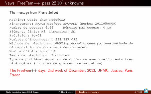
The message from Pierre Jolivet
Machine: Curie Thin Node@CEAFinancement: PRACE project HPC-PDE (number 2011050840)Nombre de coeurs: 6144 Mémoire par coeurs: 4 GoEléments finis: P3 Dimension: 2DPrécision: 1e-08Nombres d’inconnues: 1 224 387 085Méthode de résolution: GMRES préconditionné par une méthode dedécomposition de domaine à deux niveauxNombre d’itérations: 18Temps de résolution: 2 minutesType de problème: équation de diffusion avec coefficients trèshétérogènes (5 ordres de grandeur de variation)
The FreeFem++ days, 2nd week of December, 2013, UPMC, Jussieu, Paris,
France
Càdiz Numérica, June 2013, Spain. F. Hecht et al. FreeFem++ Lecture 4 / 109
Introduction
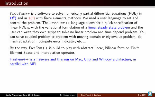
FreeFem++ is a software to solve numerically partial differential equations (PDE) inIR
2) and in IR
3) with finite elements methods. We used a user language to set andcontrol the problem. The FreeFem++ language allows for a quick specification oflinear PDE’s, with the variational formulation of a linear steady state problem and theuser can write they own script to solve no linear problem and time depend problem. Youcan solve coupled problem or problem with moving domain or eigenvalue problem, domesh adaptation , compute error indicator, etc ...
By the way, FreeFem++ is build to play with abstract linear, bilinear form on FiniteElement Space and interpolation operator.
FreeFem++ is a freeware and this run on Mac, Unix and Window architecture, inparallel with MPI.
Càdiz Numérica, June 2013, Spain. F. Hecht et al. FreeFem++ Lecture 5 / 109
History
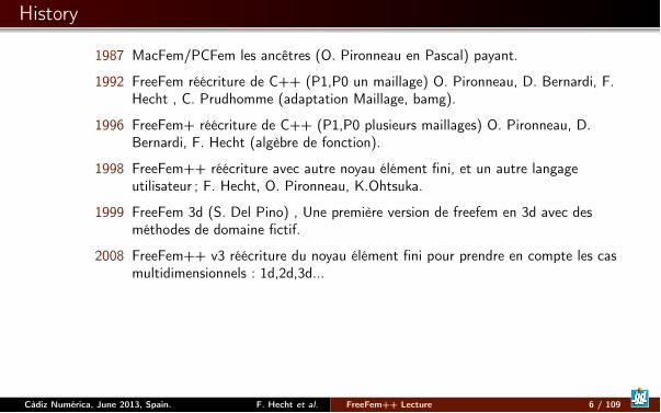
1987 MacFem/PCFem les ancêtres (O. Pironneau en Pascal) payant.
1992 FreeFem réécriture de C++ (P1,P0 un maillage) O. Pironneau, D. Bernardi, F.Hecht , C. Prudhomme (adaptation Maillage, bamg).
1996 FreeFem+ réécriture de C++ (P1,P0 plusieurs maillages) O. Pironneau, D.Bernardi, F. Hecht (algèbre de fonction).
1998 FreeFem++ réécriture avec autre noyau élément fini, et un autre langageutilisateur ; F. Hecht, O. Pironneau, K.Ohtsuka.
1999 FreeFem 3d (S. Del Pino) , Une première version de freefem en 3d avec desméthodes de domaine fictif.
2008 FreeFem++ v3 réécriture du noyau élément fini pour prendre en compte les casmultidimensionnels : 1d,2d,3d...
Càdiz Numérica, June 2013, Spain. F. Hecht et al. FreeFem++ Lecture 6 / 109
For who, for what !
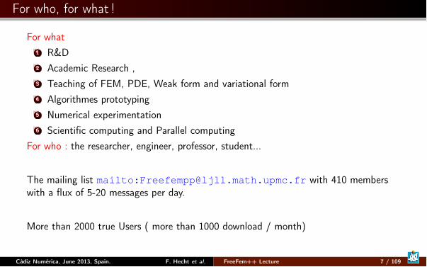
For what1 R&D2 Academic Research ,3 Teaching of FEM, PDE, Weak form and variational form4 Algorithmes prototyping5 Numerical experimentation6 Scientific computing and Parallel computing
For who : the researcher, engineer, professor, student...
The mailing list mailto:[email protected] with 410 memberswith a flux of 5-20 messages per day.
More than 2000 true Users ( more than 1000 download / month)
Càdiz Numérica, June 2013, Spain. F. Hecht et al. FreeFem++ Lecture 7 / 109
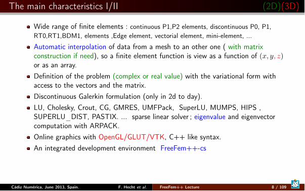
The main characteristics I/II (2D)(3D)
Wide range of finite elements : continuous P1,P2 elements, discontinuous P0, P1,RT0,RT1,BDM1, elements ,Edge element, vectorial element, mini-element, ...
Automatic interpolation of data from a mesh to an other one ( with matrixconstruction if need), so a finite element function is view as a function of (x, y, z)or as an array.Definition of the problem (complex or real value) with the variational form withaccess to the vectors and the matrix.Discontinuous Galerkin formulation (only in 2d to day).LU, Cholesky, Crout, CG, GMRES, UMFPack, SuperLU, MUMPS, HIPS ,SUPERLU_DIST, PASTIX. ... sparse linear solver ; eigenvalue and eigenvectorcomputation with ARPACK.Online graphics with OpenGL/GLUT/VTK, C++ like syntax.An integrated development environment FreeFem++-cs
Càdiz Numérica, June 2013, Spain. F. Hecht et al. FreeFem++ Lecture 8 / 109

The main characteristics II/II (2D)(3D)
Analytic description of boundaries, with specification by the user of theintersection of boundaries in 2d.Automatic mesh generator, based on the Delaunay-Voronoï algorithm. (2d,3d(tetgen) )load and save Mesh, solutionMesh adaptation based on metric, possibly anisotropic (only in 2d), with optionalautomatic computation of the metric from the Hessian of a solution. (2d,3d).Link with other soft : parview, gmsh , vtk, medit, gnuplotDynamic linking to add plugin.Full MPI interfaceNonlinear Optimisation tools : CG, Ipopt, NLOpt, stochasticWide range of examples : Navier-Stokes 3d, elasticity 3d, fluid structure, eigenvalue problem,
Schwarz’ domain decomposition algorithm, residual error indicator ...
Càdiz Numérica, June 2013, Spain. F. Hecht et al. FreeFem++ Lecture 9 / 109
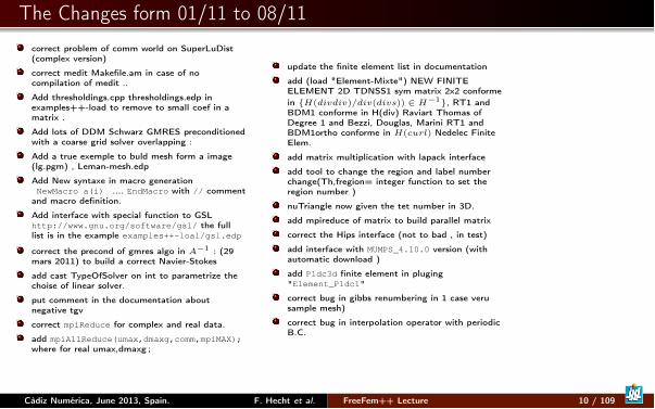
The Changes form 01/11 to 08/11correct problem of comm world on SuperLuDist(complex version)correct medit Makefile.am in case of nocompilation of medit ..Add thresholdings.cpp thresholdings.edp inexamples++-load to remove to small coef in amatrix .Add lots of DDM Schwarz GMRES preconditionedwith a coarse grid solver overlapping :Add a true exemple to buld mesh form a image(lg.pgm) , Leman-mesh.edpAdd New syntaxe in macro generationNewMacro a(i) .... EndMacro with // comment
and macro definition.Add interface with special function to GSLhttp://www.gnu.org/software/gsl/ the fulllist is in the example examples++-loal/gsl.edp
correct the precond of gmres algo in A�1 : (29mars 2011) to build a correct Navier-Stokesadd cast TypeOfSolver on int to parametrize thechoise of linear solver.put comment in the documentation aboutnegative tgvcorrect mpiReduce for complex and real data.add mpiAllReduce(umax,dmaxg,comm,mpiMAX);where for real umax,dmaxg ;
update the finite element list in documentationadd (load "Element-Mixte") NEW FINITEELEMENT 2D TDNSS1 sym matrix 2x2 conformein {H(divdiv)/div(divs)) 2 H�1}, RT1 andBDM1 conforme in H(div) Raviart Thomas ofDegree 1 and Bezzi, Douglas, Marini RT1 andBDM1ortho conforme in H(curl) Nedelec FiniteElem.add matrix multiplication with lapack interfaceadd tool to change the region and label numberchange(Th,fregion= integer function to set theregion number )nuTriangle now given the tet number in 3D.add mpireduce of matrix to build parallel matrixcorrect the Hips interface (not to bad , in test)add interface with MUMPS_4.10.0 version (withautomatic download )add P1dc3d finite element in pluging"Element_P1dc1"
correct bug in gibbs renumbering in 1 case verusample mesh)correct bug in interpolation operator with periodicB.C.
Càdiz Numérica, June 2013, Spain. F. Hecht et al. FreeFem++ Lecture 10 / 109
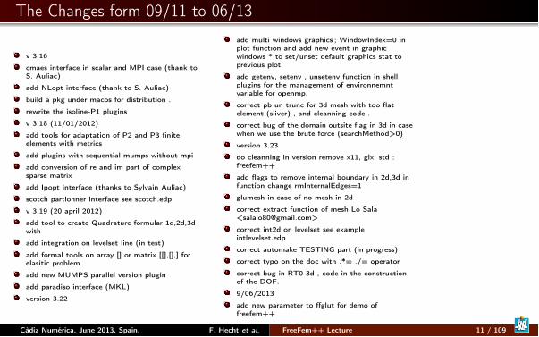
The Changes form 09/11 to 06/13
v 3.16cmaes interface in scalar and MPI case (thank toS. Auliac)add NLopt interface (thank to S. Auliac)build a pkg under macos for distribution .rewrite the isoline-P1 pluginsv 3.18 (11/01/2012)add tools for adaptation of P2 and P3 finiteelements with metricsadd plugins with sequential mumps without mpiadd conversion of re and im part of complexsparse matrixadd Ipopt interface (thanks to Sylvain Auliac)scotch partionner interface see scotch.edpv 3.19 (20 april 2012)add tool to create Quadrature formular 1d,2d,3dwithadd integration on levelset line (in test)add formal tools on array [] or matrix [[],[],] forelasitic problem.add new MUMPS parallel version pluginadd paradiso interface (MKL)version 3.22
add multi windows graphics ; WindowIndex=0 inplot function and add new event in graphicwindows * to set/unset default graphics stat toprevious plotadd getenv, setenv , unsetenv function in shellplugins for the management of environnemntvariable for openmp.correct pb un trunc for 3d mesh with too flatelement (sliver) , and cleanning code .correct bug of the domain outsite flag in 3d in casewhen we use the brute force (searchMethod>0)version 3.23do cleanning in version remove x11, glx, std :freefem++add flags to remove internal boundary in 2d,3d infunction change rmInternalEdges=1glumesh in case of no mesh in 2dcorrect extract function of mesh Lo Sala<[email protected]>correct int2d on levelset see exampleintlevelset.edpcorrect automake TESTING part (in progress)correct typo on the doc with .*= ./= operatorcorrect bug in RT0 3d , code in the constructionof the DOF.9/06/2013add new parameter to ffglut for demo offreefem++
Càdiz Numérica, June 2013, Spain. F. Hecht et al. FreeFem++ Lecture 11 / 109
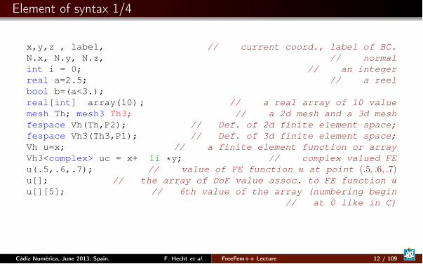
Element of syntax 1/4
x,y,z , label, // current coord., label of BC.N.x, N.y, N.z, // normalint i = 0; // an integerreal a=2.5; // a reelbool b=(a<3.);real[int] array(10); // a real array of 10 valuemesh Th; mesh3 Th3; // a 2d mesh and a 3d meshfespace Vh(Th,P2); // Def. of 2d finite element space;fespace Vh3(Th3,P1); // Def. of 3d finite element space;Vh u=x; // a finite element function or arrayVh3<complex> uc = x+ 1i *y; // complex valued FEu(.5,.6,.7); // value of FE function u at point (.5, .6, .7)u[]; // the array of DoF value assoc. to FE function uu[][5]; // 6th value of the array (numbering begin
// at 0 like in C)
Càdiz Numérica, June 2013, Spain. F. Hecht et al. FreeFem++ Lecture 12 / 109

Element of syntax 2/4
fespace V3h(Th,[P2,P2,P1]);V3h [u1,u2,p]=[x,y,z]; // a vectorial finite element
// function or array// remark u1[] <==> u2[] <==> p[] same array of unknown.
macro div(u,v) (dx(u)+dy(v))// EOM a macro// (like #define in C )
macro Grad(u) [dx(u),dy(u)] // the macro end with //varf a([u1,u2,p],[v1,v2,q])=
int2d(Th)( Grad(u1)’*Grad(v1) +Grad(u2)’*Grad(v2)-div(u1,u2)*q -div(v1,v2)*p)
+on(1,2)(u1=g1,u2=g2);
matrix A=a(V3h,V3h,solver=UMFPACK);real[int] b=a(0,V3h);u2[] =A^-1*b; // or you can put also u1[]= or p[].
Càdiz Numérica, June 2013, Spain. F. Hecht et al. FreeFem++ Lecture 13 / 109
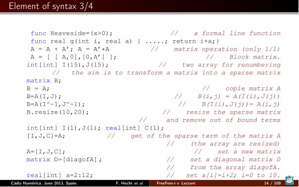
Element of syntax 3/4
func Heaveside=(x>0); // a formal line functionfunc real g(int i, real a) { .....; return i+a;}A = A + A’; A = A’*A // matrix operation (only 1/1)A = [ [ A,0],[0,A’] ]; // Block matrix.int[int] I(15),J(15); // two array for renumbering
// the aim is to transform a matrix into a sparse matrixmatrix B;B = A; // copie matrix AB=A(I,J); // B(i,j) = A(I(i),J(j))B=A(I^-1,J^-1); // B(I(i),J(j))= A(i,j)B.resize(10,20); // resize the sparse matrix
// and remove out of bound termsint[int] I(1),J(1); real[int] C(1);[I,J,C]=A; // get of the sparse term of the matrix A
// (the array are resized)A=[I,J,C]; // set a new matrixmatrix D=[diagofA]; // set a diagonal matrix D
// from the array diagofA.real[int] a=2:12; // set a[i]=i+2; i=0 to 10.
Càdiz Numérica, June 2013, Spain. F. Hecht et al. FreeFem++ Lecture 14 / 109
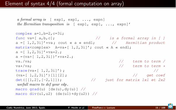
Element of syntax 4/4 (formal computation on array)
a formal array is [ exp1, exp1, ..., expn]the Hermitian transposition is [ exp1, exp1, ..., expn]’
complex a=1,b=2,c=3i;func va=[ a,b,c]; // is a formal array in [ ]a =[ 1,2,3i]’*va; cout « a « endl; // Hermitian productmatrix<complex> A=va*[ 1,2,3i]’; cout « A « endl;a =[ 1,2,3i]’*va*2.;a =(va+[ 1,2,3i])’*va*2.;va./va; // term to term /va*/va; // term to term *trace(va*[ 1,2,3i]’); //(va*[ 1,2,3i]’)[1][2]; // get coefdet([[1,2],[-2,1]]); // just for matrix 1x1 et 2x2usefull macro to def your edp.macro grad(u) [dx(u),dy(u)] //macro div(u1,u2) (dx(u1)+dy(u2)) //
Càdiz Numérica, June 2013, Spain. F. Hecht et al. FreeFem++ Lecture 15 / 109
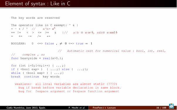
Element of syntax : Like in C
The key words are reserved
The operator like in C exempt: ^ & |+ - * / ^ // a^b= a
b
== != < > <= >= & |// a|b ⌘ a or b, a&b⌘ a and b
= += -= /= *=
BOOLEAN: 0 <=> false , 6= 0 <=> true = 1
// Automatic cast for numerical value : bool, int, reel,// complex , sofunc heavyside = real(x>0.);
for (int i=0;i<n;i++) { ...;}if ( <bool exp> ) { ...;} else { ...;};while ( <bool exp> ) { ...;}break continue key words
weakless: all local variables are almost static (????)bug if break before variable declaration in same block.bug for fespace argument or fespace function argument
Càdiz Numérica, June 2013, Spain. F. Hecht et al. FreeFem++ Lecture 16 / 109
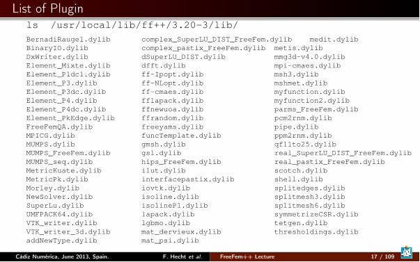
List of Pluginls /usr/local/lib/ff++/3.20-3/lib/BernadiRaugel.dylib complex_SuperLU_DIST_FreeFem.dylib medit.dylibBinaryIO.dylib complex_pastix_FreeFem.dylib metis.dylibDxWriter.dylib dSuperLU_DIST.dylib mmg3d-v4.0.dylibElement_Mixte.dylib dfft.dylib mpi-cmaes.dylibElement_P1dc1.dylib ff-Ipopt.dylib msh3.dylibElement_P3.dylib ff-NLopt.dylib mshmet.dylibElement_P3dc.dylib ff-cmaes.dylib myfunction.dylibElement_P4.dylib fflapack.dylib myfunction2.dylibElement_P4dc.dylib ffnewuoa.dylib parms_FreeFem.dylibElement_PkEdge.dylib ffrandom.dylib pcm2rnm.dylibFreeFemQA.dylib freeyams.dylib pipe.dylibMPICG.dylib funcTemplate.dylib ppm2rnm.dylibMUMPS.dylib gmsh.dylib qf11to25.dylibMUMPS_FreeFem.dylib gsl.dylib real_SuperLU_DIST_FreeFem.dylibMUMPS_seq.dylib hips_FreeFem.dylib real_pastix_FreeFem.dylibMetricKuate.dylib ilut.dylib scotch.dylibMetricPk.dylib interfacepastix.dylib shell.dylibMorley.dylib iovtk.dylib splitedges.dylibNewSolver.dylib isoline.dylib splitmesh3.dylibSuperLu.dylib isolineP1.dylib splitmesh6.dylibUMFPACK64.dylib lapack.dylib symmetrizeCSR.dylibVTK_writer.dylib lgbmo.dylib tetgen.dylibVTK_writer_3d.dylib mat_dervieux.dylib thresholdings.dylibaddNewType.dylib mat_psi.dylib
Càdiz Numérica, June 2013, Spain. F. Hecht et al. FreeFem++ Lecture 17 / 109
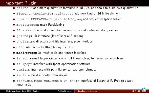
Important Pluginqf11to25 add more quadrature formulae in 1d , 2d, and tools to build own quadrature
Element_*,Morlay,BernadiRaugel add new kind of 2d finite element
SuperLu,UMFPACK64,SuperLu,MUMPS_seq add sequentiel sparse solver
metis,scotch mesh Partitioning
ffrandom true random number generator : srandomdev,srandom, random
gsl the gsl lib interface (lot of special function)
shell,pipe directory and file interface, pipe interface
dfft interface with fftw3 library for FFT.
msh3,tetgen 3d mesh tools and tetgen interface
lapack a small lacpack,interface of full linear solver, full eigen value problem.
ff-Ipopt interface with Ipopt optimisation software
ppm2rnm interface with ppm library to read ppm bitmap.
isoline build a border from isoline.
freeyams, mesh met, mmg3d-v4, medit interface of library of P. Frey to adaptmesh in 3d.
Càdiz Numérica, June 2013, Spain. F. Hecht et al. FreeFem++ Lecture 18 / 109
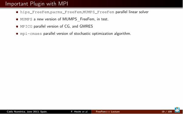
Important Plugin with MPIhips_FreeFem,parms_FreeFem,MUMPS_FreeFem parallel linear solver
MUMPS a new version of MUMPS_FreeFem, in test.
MPICG parallel version of CG, and GMRES
mpi-cmaes parallel version of stochastic optimization algorithm.
Càdiz Numérica, June 2013, Spain. F. Hecht et al. FreeFem++ Lecture 19 / 109
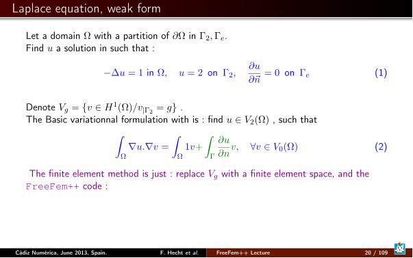
Laplace equation, weak form
Let a domain ⌦ with a partition of @⌦ in �
2
,�e
.Find u a solution in such that :
��u = 1 in ⌦, u = 2 on �
2
,@u
@~n= 0 on �
e
(1)
Denote Vg
= {v 2 H1
(⌦)/v|�2= g} .
The Basic variationnal formulation with is : find u 2 V2
(⌦) , such thatZ
⌦
ru.rv =
Z
⌦
1v+
Z
�
@u
@nv, 8v 2 V
0
(⌦) (2)
The finite element method is just : replace Vg
with a finite element space, and theFreeFem++ code :
Càdiz Numérica, June 2013, Spain. F. Hecht et al. FreeFem++ Lecture 20 / 109
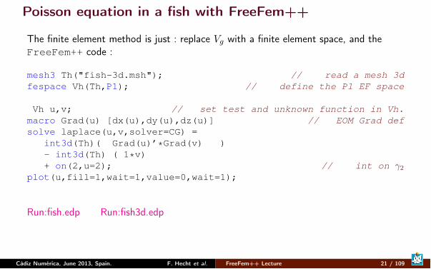
Poisson equation in a fish with FreeFem++
The finite element method is just : replace Vg
with a finite element space, and theFreeFem++ code :
mesh3 Th("fish-3d.msh"); // read a mesh 3dfespace Vh(Th,P1); // define the P1 EF space
Vh u,v; // set test and unknown function in Vh.macro Grad(u) [dx(u),dy(u),dz(u)] // EOM Grad defsolve laplace(u,v,solver=CG) =
int3d(Th)( Grad(u)’*Grad(v) )- int3d(Th) ( 1*v)+ on(2,u=2); // int on �2
plot(u,fill=1,wait=1,value=0,wait=1);
Run:fish.edp Run:fish3d.edp
Càdiz Numérica, June 2013, Spain. F. Hecht et al. FreeFem++ Lecture 21 / 109
Outline
1 Introduction
2 ToolsRemarks on weak form and boundary conditionsMesh generationBuild mesh from image3d meshMesh toolsAnisotropic Mesh adaptation
3 Academic Examples
4 Numerics Tools
5 Schwarz method with overlap
6 No Linear Problem
7 Technical Remark on freefem++
8 Phase change with Natural Convection
Càdiz Numérica, June 2013, Spain. F. Hecht et al. FreeFem++ Lecture 22 / 109

Remark on varf
The functions appearing in the variational form are formal and local to the varf definition,the only important think is the order in the parameter list, like invarf vb1([u1,u2],[q]) = int2d(Th)( (dy(u1)+dy(u2)) *q)
+int2d(Th)(1*q) + on(1,u1=2);varf vb2([v1,v2],[p]) = int2d(Th)( (dy(v1)+dy(v2)) *p)
+int2d(Th)(1*p);To build matrix A from the bilinear part the the variational form a of type varf do simply
matrix B1 = vb1(Vh,Wh [, ...] );matrix<complex> C1 = vb1(Vh,Wh [, ...] );
// where the fespace have the correct number of comp.// Vh is "fespace" for the unknown fields with 2 comp.// ex fespace Vh(Th,[P2,P2]); or fespace Vh(Th,RT);// Wh is "fespace" for the test fields with 1 comp.To build a vector, put u1 = u2 = 0 by setting 0 of on unknown part.real[int] b = vb2(0,Wh);complex[int] c = vb2(0,Wh);Remark : In this case the mesh use to defined ,
R, u, v can be different.
Càdiz Numérica, June 2013, Spain. F. Hecht et al. FreeFem++ Lecture 23 / 109
The boundary condition terms
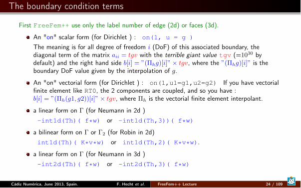
First FreeFem++ use only the label number of edge (2d) or faces (3d).
An "on" scalar form (for Dirichlet ) : on(1, u = g )
The meaning is for all degree of freedom i (DoF) of this associated boundary, thediagonal term of the matrix aii = tgv with the terrible giant value tgv (=10
30 bydefault) and the right hand side b[i] = ”(⇧hg)[i]”⇥ tgv, where the ”(⇧hg)[i]” is theboundary DoF value given by the interpolation of g.
An "on" vectorial form (for Dirichlet ) : on(1,u1=g1,u2=g2) If you have vectorialfinite element like RT0, the 2 components are coupled, and so you have :b[i] = ”(⇧h(g1, g2))[i]”⇥ tgv, where ⇧h is the vectorial finite element interpolant.
a linear form on � (for Neumann in 2d )-int1d(Th)( f*w) or -int1d(Th,3))( f*w)
a bilinear form on � or �2 (for Robin in 2d)int1d(Th)( K*v*w) or int1d(Th,2)( K*v*w).
a linear form on � (for Neumann in 3d )-int2d(Th)( f*w) or -int2d(Th,3)( f*w)
Càdiz Numérica, June 2013, Spain. F. Hecht et al. FreeFem++ Lecture 24 / 109
Build Mesh 2d
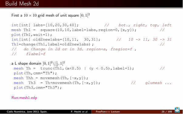
First a 10⇥ 10 grid mesh of unit square ]0, 1[2
int[int] labs=[10,20,30,40]; // bot., right, top, leftmesh Th1 = square(10,10,label=labs,region=0,[x,y]); //plot(Th1,wait=1);int[int] old2newlabs=[10,11, 30,31]; // 10 -> 11, 30 -> 31Th1=change(Th1,label=old2newlabs); //// do Change in 2d or in 3d. region=a, fregion=f ,// flabel=f
a L shape domain ]0, 1[2\[ 12 , 1[2mesh Th = trunc(Th1,(x<0.5) | (y < 0.5),label=1); //plot(Th,cmm="Th");mesh Thh = movemesh(Th,[-x,y]);mesh Th3 = Th+movemesh(Th,[-x,y]); // glumesh ...plot(Th3,cmm="Th3");
Run:mesh1.edp
Càdiz Numérica, June 2013, Spain. F. Hecht et al. FreeFem++ Lecture 25 / 109
Build Mesh 2d
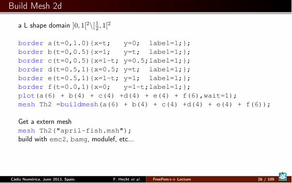
a L shape domain ]0, 1[2\[12
, 1[2
border a(t=0,1.0){x=t; y=0; label=1;};border b(t=0,0.5){x=1; y=t; label=1;};border c(t=0,0.5){x=1-t; y=0.5;label=1;};border d(t=0.5,1){x=0.5; y=t; label=1;};border e(t=0.5,1){x=1-t; y=1; label=1;};border f(t=0.0,1){x=0; y=1-t;label=1;};plot(a(6) + b(4) + c(4) +d(4) + e(4) + f(6),wait=1);mesh Th2 =buildmesh(a(6) + b(4) + c(4) +d(4) + e(4) + f(6));
Get a extern meshmesh Th2("april-fish.msh");build with emc2, bamg, modulef, etc...
Càdiz Numérica, June 2013, Spain. F. Hecht et al. FreeFem++ Lecture 26 / 109
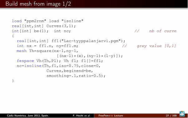
Build mesh from image 1/2
load "ppm2rnm" load "isoline"real[int,int] Curves(3,1);int[int] be(1); int nc; // nb of curve{
real[int,int] ff1("Lac-tyyppalanjarvi.pgm");int nx = ff1.n, ny=ff1.m; // grey value [0,1]mesh Th=square(nx-1,ny-1,
[(nx-1)*(x),(ny-1)*(1-y)]);fespace Vh(Th,P1); Vh f1; f1[]=ff1;nc=isoline(Th,f1,iso=0.75,close=0,
Curves,beginend=be,smoothing=.1,ratio=0.5);
}
Càdiz Numérica, June 2013, Spain. F. Hecht et al. FreeFem++ Lecture 27 / 109
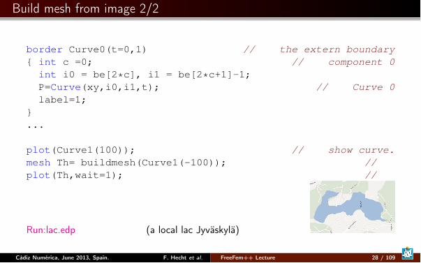
Build mesh from image 2/2
border Curve0(t=0,1) // the extern boundary{ int c =0; // component 0int i0 = be[2*c], i1 = be[2*c+1]-1;P=Curve(xy,i0,i1,t); // Curve 0label=1;
}...
plot(Curve1(100)); // show curve.mesh Th= buildmesh(Curve1(-100)); //plot(Th,wait=1); //
Run:lac.edp (a local lac Jyväskylä)
Càdiz Numérica, June 2013, Spain. F. Hecht et al. FreeFem++ Lecture 28 / 109
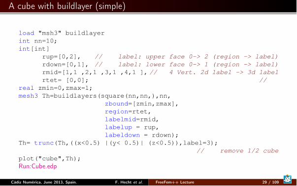
A cube with buildlayer (simple)
load "msh3" buildlayerint nn=10;int[int]
rup=[0,2], // label: upper face 0-> 2 (region -> label)rdown=[0,1], // label: lower face 0-> 1 (region -> label)rmid=[1,1 ,2,1 ,3,1 ,4,1 ], // 4 Vert. 2d label -> 3d labelrtet= [0,0]; //
real zmin=0,zmax=1;mesh3 Th=buildlayers(square(nn,nn,),nn,
zbound=[zmin,zmax],region=rtet,labelmid=rmid,labelup = rup,labeldown = rdown);
Th= trunc(Th,((x<0.5) |(y< 0.5)| (z<0.5)),label=3);// remove 1/2 cube
plot("cube",Th);Run:Cube.edp
Càdiz Numérica, June 2013, Spain. F. Hecht et al. FreeFem++ Lecture 29 / 109
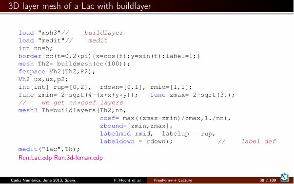
3D layer mesh of a Lac with buildlayer
load "msh3"// buildlayerload "medit"// meditint nn=5;border cc(t=0,2*pi){x=cos(t);y=sin(t);label=1;}mesh Th2= buildmesh(cc(100));fespace Vh2(Th2,P2);Vh2 ux,uz,p2;int[int] rup=[0,2], rdown=[0,1], rmid=[1,1];func zmin= 2-sqrt(4-(x*x+y*y)); func zmax= 2-sqrt(3.);// we get nn*coef layersmesh3 Th=buildlayers(Th2,nn,
coef= max((zmax-zmin)/zmax,1./nn),zbound=[zmin,zmax],labelmid=rmid, labelup = rup,labeldown = rdown); // label def
medit("lac",Th);Run:Lac.edp Run:3d-leman.edp
Càdiz Numérica, June 2013, Spain. F. Hecht et al. FreeFem++ Lecture 30 / 109

a 3d axi Mesh with buildlayer
func f=2*((.1+(((x/3))*(x-1)*(x-1)/1+x/100))^(1/3.)-(.1)^(1/3.));real yf=f(1.2,0);border up(t=1.2,0.){ x=t;y=f;label=0;}border axe2(t=0.2,1.15) { x=t;y=0;label=0;}border hole(t=pi,0) { x= 0.15 + 0.05*cos(t);y= 0.05*sin(t);
label=1;}border axe1(t=0,0.1) { x=t;y=0;label=0;}border queue(t=0,1) { x= 1.15 + 0.05*t; y = yf*t; label =0;}int np= 100;func bord= up(np)+axe1(np/10)+hole(np/10)+axe2(8*np/10)
+ queue(np/10);plot( bord); // plot the border ...mesh Th2=buildmesh(bord); // the 2d mesh axi meshplot(Th2,wait=1);int[int] l23=[0,0,1,1];Th=buildlayers(Th2,coef= max(.15,y/max(f,0.05)), 50,zbound=[0,2*pi],transfo=[x,y*cos(z),y*sin(z)],facemerge=1,labelmid=l23);
Run:3daximesh.edpCàdiz Numérica, June 2013, Spain. F. Hecht et al. FreeFem++ Lecture 31 / 109
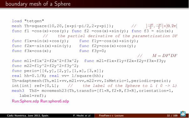
boundary mesh of a Sphere
load "tetgen"mesh Th=square(10,20,[x*pi-pi/2,2*y*pi]); // ]
�pi2 , �pi
2 [⇥]0, 2⇡[func f1 =cos(x)*cos(y); func f2 =cos(x)*sin(y); func f3 = sin(x);
// the partiel derivative of the parametrization DFfunc f1x=sin(x)*cos(y); func f1y=-cos(x)*sin(y);func f2x=-sin(x)*sin(y); func f2y=cos(x)*cos(y);func f3x=cos(x); func f3y=0;
// M = DF tDFfunc m11=f1x^2+f2x^2+f3x^2; func m21=f1x*f1y+f2x*f2y+f3x*f3y;func m22=f1y^2+f2y^2+f3y^2;func perio=[[4,y],[2,y],[1,x],[3,x]];real hh=0.1/R; real vv= 1/square(hh);Th=adaptmesh(Th,m11*vv,m21*vv,m22*vv,IsMetric=1,periodic=perio);int[int] ref=[0,L]; // the label of the Sphere to L ( 0 -> L)mesh3 ThS= movemesh23(Th,transfo=[f1*R,f2*R,f3*R],orientation=1,
label=ref);Run:Sphere.edp Run:sphere6.edp
Càdiz Numérica, June 2013, Spain. F. Hecht et al. FreeFem++ Lecture 32 / 109

Build 3d Mesh from boundary mesh
include "MeshSurface.idp" // tool for 3d surfaces meshesmesh3 Th;try { Th=readmesh3("Th-hex-sph.mesh"); } // try to readcatch(...) { // catch a reading error so build the mesh...
real hs = 0.2; // mesh size on sphereint[int] NN=[11,9,10];real [int,int] BB=[[-1.1,1.1],[-.9,.9],[-1,1]]; // Mesh Boxint [int,int] LL=[[1,2],[3,4],[5,6]]; // Label Boxmesh3 ThHS = SurfaceHex(NN,BB,LL,1)+Sphere(0.5,hs,7,1);
// surface meshesreal voltet=(hs^3)/6.; // volume mesh control.real[int] domaine = [0,0,0,1,voltet,0,0,0.7,2,voltet];Th = tetg(ThHS,switch="pqaAAYYQ",
nbofregions=2,regionlist=domaine);savemesh(Th,"Th-hex-sph.mesh"); } // save for next run
Càdiz Numérica, June 2013, Spain. F. Hecht et al. FreeFem++ Lecture 33 / 109

Mesh tools
change to change label and region numbering in 2d and 3d.movemesh checkmovemesh movemesh23 movemesh3
triangulate (2d) , tetgconvexhull (3d) build mesh mesh for a set of pointemptymesh (2d) built a empty mesh for Lagrange multiplierfreeyams to optimize surface meshmmg3d to optimize volume mesh with constant surface meshmshmet to compute metricisoline to extract isoline (2d)trunc to remove peace of mesh and split all element (2d,3d)splitmesh to split 2d mesh in no regular way.
Càdiz Numérica, June 2013, Spain. F. Hecht et al. FreeFem++ Lecture 34 / 109
Metric / unit Mesh
In Euclidean geometry the length |�| of a curve � of Rd parametrized by �(t)t=0..1 is
|�| =Z
1
0
p< �0(t), �0(t) >dt
We introduce the metric M(x) as a field of d⇥ d symmetric positive definite matrices,and the length ` of � w.r.t M is :
` =
Z1
0
p< �0(t),M(�(t))�0(t) >dt
The key-idea is to construct a mesh where the lengths of the edges are close to 1accordingly to M.
Càdiz Numérica, June 2013, Spain. F. Hecht et al. FreeFem++ Lecture 35 / 109
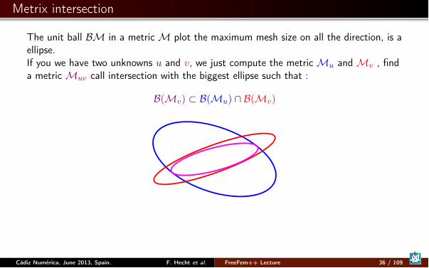
Metrix intersection
The unit ball BM in a metric M plot the maximum mesh size on all the direction, is aellipse.If you we have two unknowns u and v, we just compute the metric M
u
and Mv
, finda metric M
uv
call intersection with the biggest ellipse such that :
B(Mv
) ⇢ B(Mu
) \ B(Mv
)
Càdiz Numérica, June 2013, Spain. F. Hecht et al. FreeFem++ Lecture 36 / 109
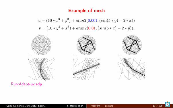
Example of mesh
u = (10 ⇤ x3 + y3) + atan2(0.001, (sin(5 ⇤ y)� 2 ⇤ x))v = (10 ⇤ y3 + x3) + atan2(0.01, (sin(5 ⇤ x)� 2 ⇤ y)).
Enter ? for help Enter ? for help Enter ? for help
Run:Adapt-uv.edp
Càdiz Numérica, June 2013, Spain. F. Hecht et al. FreeFem++ Lecture 37 / 109
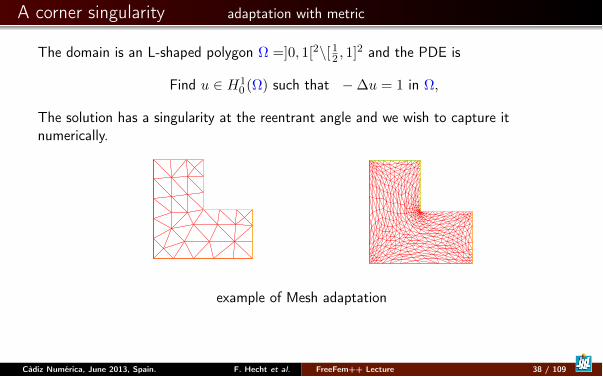
A corner singularity adaptation with metric
The domain is an L-shaped polygon ⌦ =]0, 1[2\[12
, 1]2 and the PDE is
Find u 2 H1
0
(⌦) such that ��u = 1 in ⌦,
The solution has a singularity at the reentrant angle and we wish to capture itnumerically.
example of Mesh adaptation
Càdiz Numérica, June 2013, Spain. F. Hecht et al. FreeFem++ Lecture 38 / 109
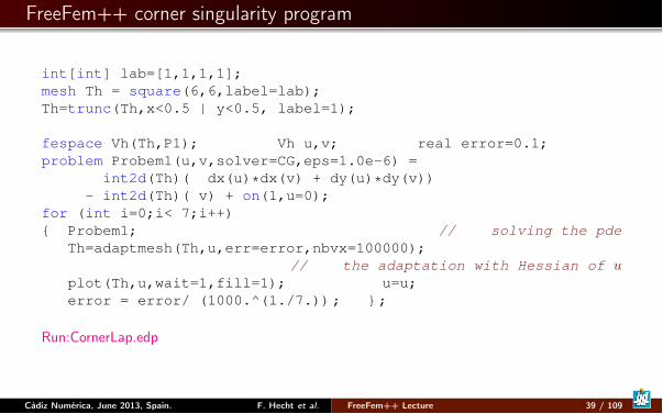
FreeFem++ corner singularity program
int[int] lab=[1,1,1,1];mesh Th = square(6,6,label=lab);Th=trunc(Th,x<0.5 | y<0.5, label=1);
fespace Vh(Th,P1); Vh u,v; real error=0.1;problem Probem1(u,v,solver=CG,eps=1.0e-6) =
int2d(Th)( dx(u)*dx(v) + dy(u)*dy(v))- int2d(Th)( v) + on(1,u=0);
for (int i=0;i< 7;i++){ Probem1; // solving the pde
Th=adaptmesh(Th,u,err=error,nbvx=100000);// the adaptation with Hessian of u
plot(Th,u,wait=1,fill=1); u=u;error = error/ (1000.^(1./7.)); };
Run:CornerLap.edp
Càdiz Numérica, June 2013, Spain. F. Hecht et al. FreeFem++ Lecture 39 / 109
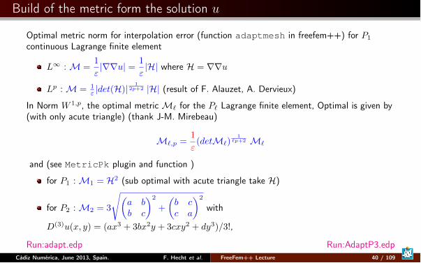
Build of the metric form the solution u
Optimal metric norm for interpolation error (function adaptmesh in freefem++) for P1
continuous Lagrange finite element
L1 : M =
1
"|rru| = 1
"|H| where H = rru
Lp : M =
1" |det(H)| 1
2p+2 |H| (result of F. Alauzet, A. Dervieux)
In Norm W 1,p, the optimal metric M` for the P` Lagrange finite element, Optimal is given by(with only acute triangle) (thank J-M. Mirebeau)
M`,p =
1
"(detM`)
1`p+2 M`
and (see MetricPk plugin and function )
for P1 : M1 = H2 (sub optimal with acute triangle take H)
for P2 : M2 = 3
s✓a bb c
◆2
+
✓b cc a
◆2
with
D(3)u(x, y) = (ax3+ 3bx2y + 3cxy2 + dy3)/3!,
Run:adapt.edp Run:AdaptP3.edpCàdiz Numérica, June 2013, Spain. F. Hecht et al. FreeFem++ Lecture 40 / 109
Outline
1 Introduction
2 Tools
3 Academic ExamplesLaplace/Poisson3d Poisson equation with mesh adaptationLinear PDELinear elasticty equationStokes equationOptimize Time depend schema
4 Numerics Tools
5 Schwarz method with overlap
6 No Linear Problem
7 Technical Remark on freefem++
8 Phase change with Natural Convection
Càdiz Numérica, June 2013, Spain. F. Hecht et al. FreeFem++ Lecture 41 / 109
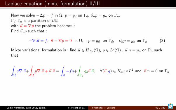
Laplace equation (mixte formulation) II/III
Now we solve ��p = f in ⌦, p = gd
on �
d
, @n
p = gn
on �
n
.�
d
,�n
is a partition of @⌦.with ~u = rp the problem becomes :Find ~u, p such that :
�r.~u = f, ~u�rp = 0 in ⌦, p = gd
on �
d
, @n
p = gn
on �
n
(3)
Mixte variational formulation is : find ~u 2 Hdiv
(⌦), p 2 L2
(⌦) , ~u.n = gn
on �
n
suchthat
Z
⌦
qr.~u+
Z
⌦
pr.~v + ~u.~v =
Z
⌦
�fq+
Z
�d
gd
~v.~n, 8(~v, q) 2 Hdiv
⇥L2, and ~v.n = 0 on �
n
Càdiz Numérica, June 2013, Spain. F. Hecht et al. FreeFem++ Lecture 42 / 109
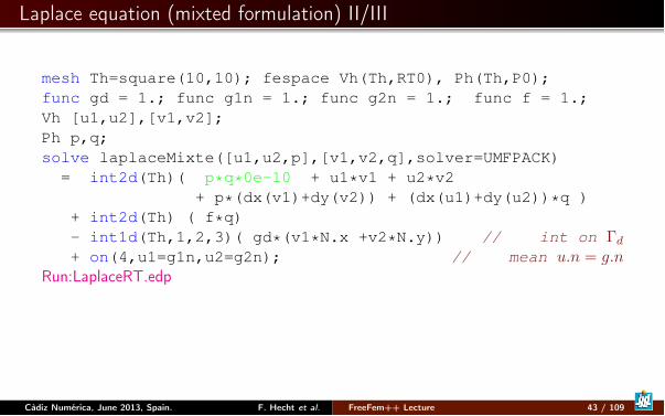
Laplace equation (mixted formulation) II/III
mesh Th=square(10,10); fespace Vh(Th,RT0), Ph(Th,P0);func gd = 1.; func g1n = 1.; func g2n = 1.; func f = 1.;Vh [u1,u2],[v1,v2];Ph p,q;solve laplaceMixte([u1,u2,p],[v1,v2,q],solver=UMFPACK)= int2d(Th)( p*q*0e-10 + u1*v1 + u2*v2
+ p*(dx(v1)+dy(v2)) + (dx(u1)+dy(u2))*q )+ int2d(Th) ( f*q)- int1d(Th,1,2,3)( gd*(v1*N.x +v2*N.y)) // int on �
d
+ on(4,u1=g1n,u2=g2n); // mean u.n = g.nRun:LaplaceRT.edp
Càdiz Numérica, June 2013, Spain. F. Hecht et al. FreeFem++ Lecture 43 / 109
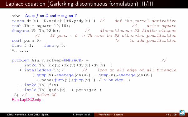
Laplace equation (Garlerking discontinuous formulation) III/III
solve ��u = f on ⌦ and u = g on �
macro dn(u) (N.x*dx(u)+N.y*dy(u) ) // def the normal derivativemesh Th = square(10,10); // unite squarefespace Vh(Th,P2dc); // discontinuous P2 finite element
// if pena = 0 => Vh must be P2 otherwise penalizationreal pena=0; // to add penalizationfunc f=1; func g=0;Vh u,v;
problem A(u,v,solver=UMFPACK) = //int2d(Th)(dx(u)*dx(v)+dy(u)*dy(v) )
+ intalledges(Th)( // loop on all edge of all triangle( jump(v)*average(dn(u)) - jump(u)*average(dn(v))
+ pena*jump(u)*jump(v) ) / nTonEdge )- int2d(Th)(f*v)- int1d(Th)(g*dn(v) + pena*g*v);
A; // solve DGRun:LapDG2.edp
Càdiz Numérica, June 2013, Spain. F. Hecht et al. FreeFem++ Lecture 44 / 109
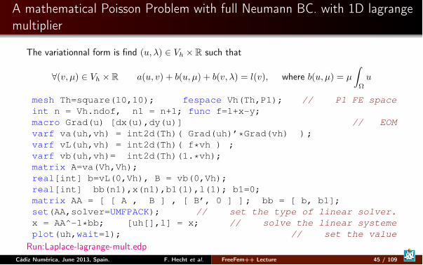
A mathematical Poisson Problem with full Neumann BC. with 1D lagrangemultiplier
The variationnal form is find (u,�) 2 Vh ⇥ R such that
8(v, µ) 2 Vh ⇥ R a(u, v) + b(u, µ) + b(v,�) = l(v), where b(u, µ) = µ
Z
⌦u
mesh Th=square(10,10); fespace Vh(Th,P1); // P1 FE spaceint n = Vh.ndof, n1 = n+1; func f=1+x-y;macro Grad(u) [dx(u),dy(u)] // EOMvarf va(uh,vh) = int2d(Th)( Grad(uh)’*Grad(vh) );varf vL(uh,vh) = int2d(Th)( f*vh ) ;varf vb(uh,vh)= int2d(Th)(1.*vh);matrix A=va(Vh,Vh);real[int] b=vL(0,Vh), B = vb(0,Vh);real[int] bb(n1),x(n1),b1(1),l(1); b1=0;matrix AA = [ [ A , B ] , [ B’, 0 ] ]; bb = [ b, b1];set(AA,solver=UMFPACK); // set the type of linear solver.x = AA^-1*bb; [uh[],l] = x; // solve the linear systemeplot(uh,wait=1); // set the value
Run:Laplace-lagrange-mult.edpCàdiz Numérica, June 2013, Spain. F. Hecht et al. FreeFem++ Lecture 45 / 109
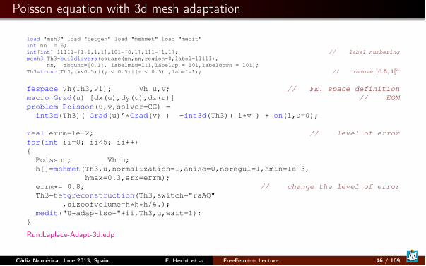
Poisson equation with 3d mesh adaptation
load "msh3" load "tetgen" load "mshmet" load "medit"int nn = 6;int[int] l1111=[1,1,1,1],l01=[0,1],l11=[1,1]; // label numberingmesh3 Th3=buildlayers(square(nn,nn,region=0,label=l1111),
nn, zbound=[0,1], labelmid=l11,labelup = l01,labeldown = l01);Th3=trunc(Th3,(x<0.5)|(y < 0.5)|(z < 0.5) ,label=1); // remove ]0.5, 1[3
fespace Vh(Th3,P1); Vh u,v; // FE. space definitionmacro Grad(u) [dx(u),dy(u),dz(u)] // EOMproblem Poisson(u,v,solver=CG) =
int3d(Th3)( Grad(u)’*Grad(v) ) -int3d(Th3)( 1*v ) + on(1,u=0);
real errm=1e-2; // level of errorfor(int ii=0; ii<5; ii++){
Poisson; Vh h;h[]=mshmet(Th3,u,normalization=1,aniso=0,nbregul=1,hmin=1e-3,
hmax=0.3,err=errm);errm*= 0.8; // change the level of errorTh3=tetgreconstruction(Th3,switch="raAQ"
,sizeofvolume=h*h*h/6.);medit("U-adap-iso-"+ii,Th3,u,wait=1);
}
Run:Laplace-Adapt-3d.edp
Càdiz Numérica, June 2013, Spain. F. Hecht et al. FreeFem++ Lecture 46 / 109
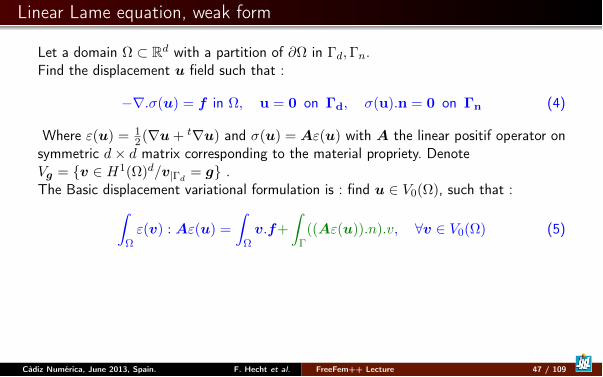
Linear Lame equation, weak form
Let a domain ⌦ ⇢ Rd with a partition of @⌦ in �
d
,�n
.Find the displacement u field such that :
�r.�(u) = f in ⌦, u = 0 on �d, �(u).n = 0 on �n (4)
Where "(u) = 1
2
(ru+
tru) and �(u) = A"(u) with A the linear positif operator onsymmetric d⇥ d matrix corresponding to the material propriety. DenoteVg = {v 2 H1
(⌦)
d/v|�d= g} .
The Basic displacement variational formulation is : find u 2 V0
(⌦), such that :Z
⌦
"(v) : A"(u) =
Z
⌦
v.f+
Z
�
((A"(u)).n).v, 8v 2 V0
(⌦) (5)
Càdiz Numérica, June 2013, Spain. F. Hecht et al. FreeFem++ Lecture 47 / 109
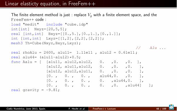
Linear elasticty equation, in FreeFem++
The finite element method is just : replace Vg
with a finite element space, and theFreeFem++ code :load "medit" include "cube.idp"int[int] Nxyz=[20,5,5];real [int,int] Bxyz=[[0.,5.],[0.,1.],[0.,1.]];int [int,int] Lxyz=[[1,2],[2,2],[2,2]];mesh3 Th=Cube(Nxyz,Bxyz,Lxyz);
// Alu ...real rhoAlu = 2600, alu11= 1.11e11 , alu12 = 0.61e11;real alu44= (alu11-alu12)*0.5;func Aalu = [ [alu11, alu12,alu12, 0. ,0. ,0. ],
[alu12, alu11,alu12, 0. ,0. ,0. ],[alu12, alu12,alu11, 0. ,0. ,0. ],[0. , 0. , 0. , alu44,0. ,0. ],[0. , 0. , 0. , 0. ,alu44,0. ],[0. , 0. , 0. , 0. ,0. ,alu44] ];
real gravity = -9.81;
Càdiz Numérica, June 2013, Spain. F. Hecht et al. FreeFem++ Lecture 48 / 109
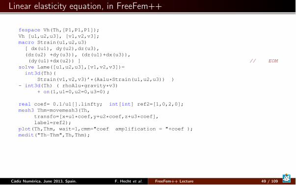
Linear elasticity equation, in FreeFem++
fespace Vh(Th,[P1,P1,P1]);Vh [u1,u2,u3], [v1,v2,v3];macro Strain(u1,u2,u3)
[ dx(u1), dy(u2),dz(u3),(dz(u2) +dy(u3)), (dz(u1)+dx(u3)),(dy(u1)+dx(u2)) ] // EOM
solve Lame([u1,u2,u3],[v1,v2,v3])=int3d(Th)(
Strain(v1,v2,v3)’*(Aalu*Strain(u1,u2,u3)) )- int3d(Th) ( rhoAlu*gravity*v3)
+ on(1,u1=0,u2=0,u3=0);
real coef= 0.1/u1[].linfty; int[int] ref2=[1,0,2,0];mesh3 Thm=movemesh3(Th,
transfo=[x+u1*coef,y+u2*coef,z+u3*coef],label=ref2);
plot(Th,Thm, wait=1,cmm="coef amplification = "+coef );medit("Th-Thm",Th,Thm);
Càdiz Numérica, June 2013, Spain. F. Hecht et al. FreeFem++ Lecture 49 / 109
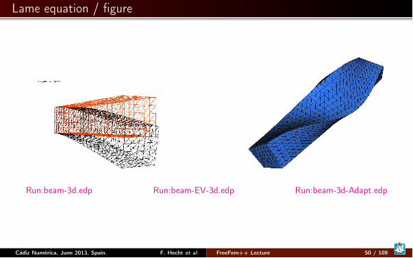
Lame equation / figure
Run:beam-3d.edp Run:beam-EV-3d.edp Run:beam-3d-Adapt.edp
Càdiz Numérica, June 2013, Spain. F. Hecht et al. FreeFem++ Lecture 50 / 109
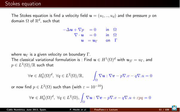
Stokes equation
The Stokes equation is find a velocity field u = (u1
, .., ud
) and the pressure p ondomain ⌦ of Rd, such that
��u+rp = 0 in ⌦
r · u = 0 in ⌦
u = u�
on �
where u�
is a given velocity on boundary �.The classical variational formulation is : Find u 2 H1
(⌦)
d with u|� = u�
, andp 2 L2
(⌦)/R such that
8v 2 H1
0
(⌦)
d, 8q 2 L2
(⌦)/R,Z
⌦
ru : rv � pr.v � qr.u = 0
or now find p 2 L2
(⌦) such than (with " = 10
�10)
8v 2 H1
0
(⌦)
d, 8q 2 L2
(⌦),
Z
⌦
ru : rv � pr.v � qr.u+ "pq = 0
Càdiz Numérica, June 2013, Spain. F. Hecht et al. FreeFem++ Lecture 51 / 109
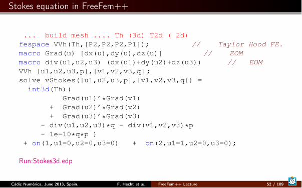
Stokes equation in FreeFem++
... build mesh .... Th (3d) T2d ( 2d)fespace VVh(Th,[P2,P2,P2,P1]); // Taylor Hood FE.macro Grad(u) [dx(u),dy(u),dz(u)] // EOMmacro div(u1,u2,u3) (dx(u1)+dy(u2)+dz(u3)) // EOMVVh [u1,u2,u3,p],[v1,v2,v3,q];solve vStokes([u1,u2,u3,p],[v1,v2,v3,q]) =int3d(Th)(
Grad(u1)’*Grad(v1)+ Grad(u2)’*Grad(v2)+ Grad(u3)’*Grad(v3)
- div(u1,u2,u3)*q - div(v1,v2,v3)*p- 1e-10*q*p )
+ on(1,u1=0,u2=0,u3=0) + on(2,u1=1,u2=0,u3=0);
Run:Stokes3d.edp
Càdiz Numérica, June 2013, Spain. F. Hecht et al. FreeFem++ Lecture 52 / 109
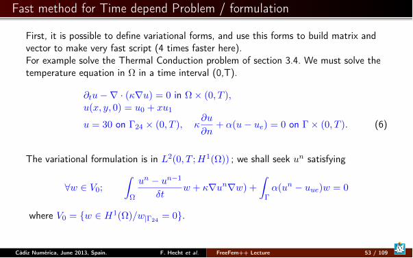
Fast method for Time depend Problem / formulation
First, it is possible to define variational forms, and use this forms to build matrix andvector to make very fast script (4 times faster here).For example solve the Thermal Conduction problem of section 3.4. We must solve thetemperature equation in ⌦ in a time interval (0,T).
@t
u�r · (ru) = 0 in ⌦⇥ (0, T ),u(x, y, 0) = u
0
+ xu1
u = 30 on �
24
⇥ (0, T ), @u
@n+ ↵(u� u
e
) = 0 on �⇥ (0, T ). (6)
The variational formulation is in L2
(0, T ;H1
(⌦)) ; we shall seek un satisfying
8w 2 V0
;
Z
⌦
un � un�1
�tw + runrw) +
Z
�
↵(un � uue
)w = 0
where V0
= {w 2 H1
(⌦)/w|�24= 0}.
Càdiz Numérica, June 2013, Spain. F. Hecht et al. FreeFem++ Lecture 53 / 109
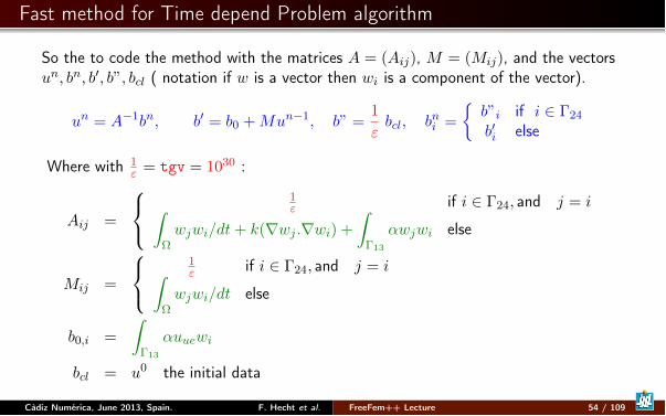
Fast method for Time depend Problem algorithm
So the to code the method with the matrices A = (Aij
), M = (Mij
), and the vectorsun, bn, b0, b”, b
cl
( notation if w is a vector then wi
is a component of the vector).
un = A�1bn, b0 = b0
+Mun�1, b” =
1
"bcl
, bni
=
⇢b”
i
if i 2 �
24
b0i
else
Where with 1
"
= tgv = 10
30 :
Aij
=
8<
:
1
"
if i 2 �
24
, and j = iZ
⌦
wj
wi
/dt+ k(rwj
.rwi
) +
Z
�13
↵wj
wi
else
Mij
=
8<
:
1
"
if i 2 �
24
, and j = iZ
⌦
wj
wi
/dt else
b0,i
=
Z
�13
↵uue
wi
bcl
= u0 the initial data
Càdiz Numérica, June 2013, Spain. F. Hecht et al. FreeFem++ Lecture 54 / 109
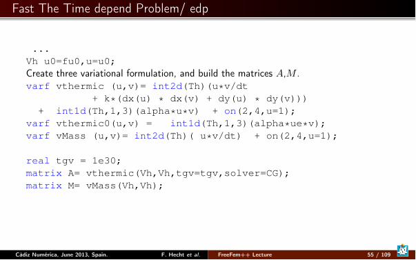
Fast The Time depend Problem/ edp
...Vh u0=fu0,u=u0;Create three variational formulation, and build the matrices A,M .varf vthermic (u,v)= int2d(Th)(u*v/dt
+ k*(dx(u) * dx(v) + dy(u) * dy(v)))+ int1d(Th,1,3)(alpha*u*v) + on(2,4,u=1);
varf vthermic0(u,v) = int1d(Th,1,3)(alpha*ue*v);varf vMass (u,v)= int2d(Th)( u*v/dt) + on(2,4,u=1);
real tgv = 1e30;matrix A= vthermic(Vh,Vh,tgv=tgv,solver=CG);matrix M= vMass(Vh,Vh);
Càdiz Numérica, June 2013, Spain. F. Hecht et al. FreeFem++ Lecture 55 / 109
Fast The Time depend Problem/ edp
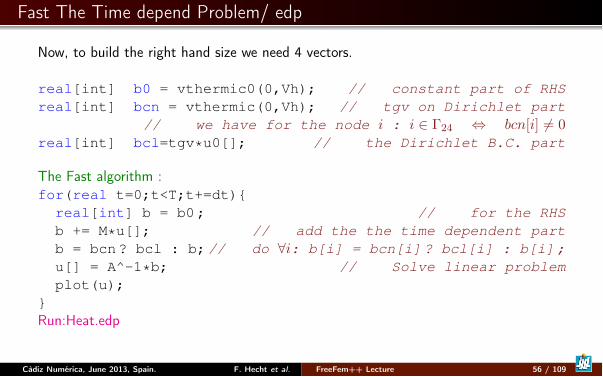
Now, to build the right hand size we need 4 vectors.
real[int] b0 = vthermic0(0,Vh); // constant part of RHSreal[int] bcn = vthermic(0,Vh); // tgv on Dirichlet part
// we have for the node i : i 2 �
24
, bcn[i] 6= 0
real[int] bcl=tgv*u0[]; // the Dirichlet B.C. part
The Fast algorithm :for(real t=0;t<T;t+=dt){real[int] b = b0; // for the RHSb += M*u[]; // add the the time dependent partb = bcn? bcl : b;// do 8i: b[i] = bcn[i]? bcl[i] : b[i];u[] = A^-1*b; // Solve linear problemplot(u);
}Run:Heat.edp
Càdiz Numérica, June 2013, Spain. F. Hecht et al. FreeFem++ Lecture 56 / 109

Outline
1 Introduction
2 Tools
3 Academic Examples
4 Numerics ToolsConnectivityInput/OutputEigenvalueEigenvalue/ EigenvectorOptimization ToolsMPI/Parallel
5 Schwarz method with overlap
6 No Linear Problem
7 Technical Remark on freefem++
8 Phase change with Natural Convection
Càdiz Numérica, June 2013, Spain. F. Hecht et al. FreeFem++ Lecture 57 / 109
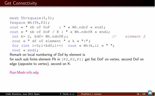
Get Connectivity
mesh Th=square(5,5);fespace Wh(Th,P2);cout « " nb of DoF : " « Wh.ndof « endl;cout « " nb of DoF / K : " « Wh.ndofK « endl;int k= 2, kdf= Wh.ndofK;; // element 2cout « " df of element " « k « ":";for (int i=0;i<kdf;i++) cout « Wh(k,i) « " ";cout « endl;
Remark on local numbering of Dof by element isfor each sub finite element Pk in [P2,P2,P1] get fist DoF on vertex, second Dof onedge (opposite to vertex), second on K.
Run:Mesh-info.edp
Càdiz Numérica, June 2013, Spain. F. Hecht et al. FreeFem++ Lecture 58 / 109
Save/Restore
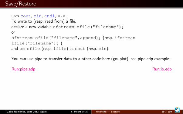
uses cout, cin, endl, «,».To write to (resp. read from) a file,declare a new variable ofstream ofile("filename");orofstream ofile("filename",append); (resp. ifstreamifile("filename"); )and use ofile (resp. ifile) as cout (resp. cin).
You can use pipe to transfer data to a other code here (gnuplot), see pipe.edp example :
Run:pipe.edp Run:io.edp
Càdiz Numérica, June 2013, Spain. F. Hecht et al. FreeFem++ Lecture 59 / 109
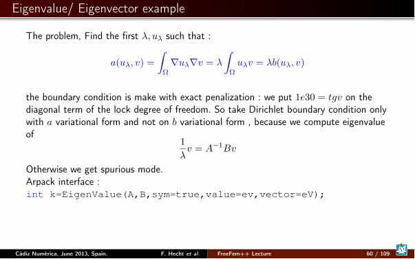
Eigenvalue/ Eigenvector example
The problem, Find the first �, u�
such that :
a(u�
, v) =
Z
⌦
ru�
rv = �
Z
⌦
u�
v = �b(u�
, v)
the boundary condition is make with exact penalization : we put 1e30 = tgv on thediagonal term of the lock degree of freedom. So take Dirichlet boundary condition onlywith a variational form and not on b variational form , because we compute eigenvalueof
1
�v = A�1Bv
Otherwise we get spurious mode.Arpack interface :int k=EigenValue(A,B,sym=true,value=ev,vector=eV);
Càdiz Numérica, June 2013, Spain. F. Hecht et al. FreeFem++ Lecture 60 / 109
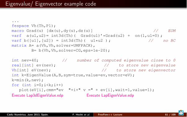
Eigenvalue/ Eigenvector example code
...fespace Vh(Th,P1);macro Grad(u) [dx(u),dy(u),dz(u)] // EOMvarf a(u1,u2)= int3d(Th)( Grad(u1)’*Grad(u2) + on(1,u1=0);varf b([u1],[u2]) = int3d(Th)( u1*u2 ); // no BCmatrix A= a(Vh,Vh,solver=UMFPACK),
B= b(Vh,Vh,solver=CG,eps=1e-20);
int nev=40; // number of computed eigenvalue close to 0real[int] ev(nev); // to store nev eigenvalueVh[int] eV(nev); // to store nev eigenvectorint k=EigenValue(A,B,sym=true,value=ev,vector=eV);k=min(k,nev);for (int i=0;i<k;i++)
plot(eV[i],cmm="ev "+i+" v =" + ev[i],wait=1,value=1);Execute Lap3dEigenValue.edp Execute LapEigenValue.edp
Càdiz Numérica, June 2013, Spain. F. Hecht et al. FreeFem++ Lecture 61 / 109
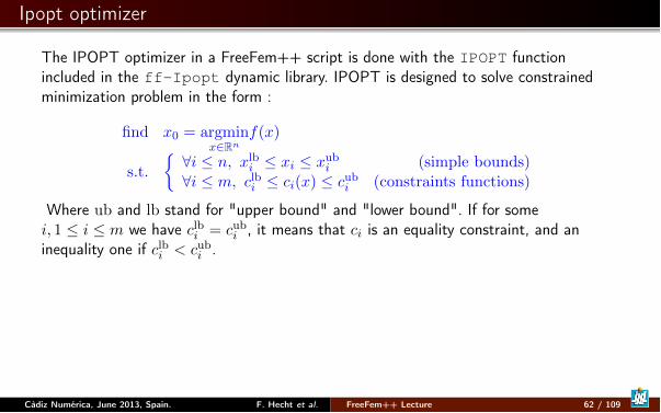
Ipopt optimizer
The IPOPT optimizer in a FreeFem++ script is done with the IPOPT functionincluded in the ff-Ipopt dynamic library. IPOPT is designed to solve constrainedminimization problem in the form :
find x0
= argmin
x2Rnf(x)
s.t.
⇢ 8i n, xlbi
xi
xubi
(simple bounds)
8i m, clbi
ci
(x) cubi
(constraints functions)
Where ub and lb stand for "upper bound" and "lower bound". If for somei, 1 i m we have clb
i
= cubi
, it means that ci
is an equality constraint, and aninequality one if clb
i
< cubi
.
Càdiz Numérica, June 2013, Spain. F. Hecht et al. FreeFem++ Lecture 62 / 109

Ipopt Data, next
func real J(real[int] &X) {...} // Fitness Function,func real[int] gradJ(real[int] &X) {...} // Gradient
func real[int] C(real[int] &X) {...} // Constraintsfunc matrix jacC(real[int] &X) {...} // Constraints jacobian
matrix jacCBuffer; // just declare, no need to define yetfunc matrix jacC(real[int] &X){... // fill jacCBufferreturn jacCBuffer;
}The hessian returning function is somewhat different because it has to be the hessian of the lagrangian
function : (x,�f ,�) 7! �fr2f(x) +
mX
i=1
�ir2ci(x) where � 2 Rm and � 2 R. Your hessian function should
then have the following prototype :matrix hessianLBuffer; // just to keep it in mindfunc matrix hessianL(real[int] &X,real sigma,real[int] &lambda) {...}
Càdiz Numérica, June 2013, Spain. F. Hecht et al. FreeFem++ Lecture 63 / 109
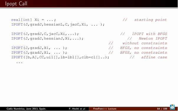
Ipopt Call
real[int] Xi = ...; // starting pointIPOPT(J,gradJ,hessianL,C,jacC,Xi, ... );
IPOPT(J,gradJ,C,jacC,Xi,...); // IPOPT with BFGSIPOPT(J,gradJ,hessianJ,Xi,...); // Newton IPOPT
// without constraintsIPOPT(J,gradJ,Xi, ... ); // BFGS, no constraintsIPOPT(J,gradJ,Xi, ... ); // BFGS, no constraintsIPOPT([b,A],CC,ui1[],lb=lb1[],clb=cl[]..); // affine case
...
Càdiz Numérica, June 2013, Spain. F. Hecht et al. FreeFem++ Lecture 64 / 109
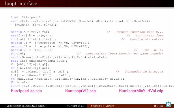
Ipopt interface
load "ff-Ipopt"varf vP([u1,u2],[v1,v2]) = int2d(Th)(Grad(u1)’*Grad(v1)+ Grad(u2)’*Grad(v2))- int2d(Th)(f1*v1+f2*v2);
matrix A = vP(Vh,Vh); // Fitness function matrix...real[int] b = vP(0,Vh); // and linear formint[int] II1=[0],II2=[1]; // Constraints matrixmatrix C1 = interpolate (Wh,Vh, U2Vc=II1);matrix C2 = interpolate (Wh,Vh, U2Vc=II2);matrix CC = -1*C1 + C2; // u2 - u1 >0Wh cl=0; // constraints lower bounds (no upper bounds)varf vGamma([u1,u2],[v1,v2]) = on(1,2,3,4,u1=1,u2=1);real[int] onGamma=vGamma(0,Vh);Vh [ub1,ub2]=[g1,g2];Vh [lb1,lb2]=[g1,g2];ub1[] = onGamma? ub1[] : 1e19 ; // Unbounded in interiorlb1[] = onGamma? lb1[] : -1e19 ;Vh [uzi,uzi2]=[uz,uz2],[lzi,lzi2]=[lz,lz2],[ui1,ui2]=[u1,u2];;Wh lmi=lm;IPOPT([b,A],CC,ui1[],lb=lb1[],clb=cl[],ub=ub1[],warmstart=iter>1,uz=uzi[],lz=lzi[],lm=lmi[]);
Run:IpoptLap.edp Run:IpoptVI2.edp Run:IpoptMinSurfVol.edp
Càdiz Numérica, June 2013, Spain. F. Hecht et al. FreeFem++ Lecture 65 / 109

NLopt interface WARNING : use full matrix
load "ff-NLopt"...if(kas==1)
mini = nloptAUGLAG(J,start,grad=dJ,lb=lo,ub=up,IConst=IneqC,gradIConst=dIneqC,subOpt="LBFGS",stopMaxFEval=10000,stopAbsFTol=starttol);
else if(kas==2)mini = nloptMMA(J,start,grad=dJ,lb=lo,ub=up,stopMaxFEval=10000,
stopAbsFTol=starttol);else if(kas==3)
mini = nloptAUGLAG(J,start,grad=dJ,IConst=IneqC,gradIConst=dIneqC,EConst=BC,gradEConst=dBC,subOpt="LBFGS",stopMaxFEval=200,stopRelXTol=1e-2);
else if(kas==4)mini = nloptSLSQP(J,start,grad=dJ,IConst=IneqC,gradIConst=dIneqC,
EConst=BC,gradEConst=dBC,stopMaxFEval=10000,stopAbsFTol=starttol);
Run:VarIneq2.edp
Càdiz Numérica, June 2013, Spain. F. Hecht et al. FreeFem++ Lecture 66 / 109
Stochastic interface
This algorithm works with a normal multivariate distribution in the parameters spaceand try to adapt its covariance matrix using the information provides by the successivefunction evaluations. Syntaxe : cmaes(J,u[],..) ( )From http://www.lri.fr/~hansen/javadoc/fr/inria/optimization/cmaes/package-summary.html
Càdiz Numérica, June 2013, Spain. F. Hecht et al. FreeFem++ Lecture 67 / 109
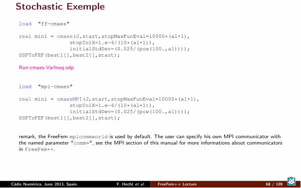
Stochastic Exemple
load "ff-cmaes"
real mini = cmaes(J,start,stopMaxFunEval=10000*(al+1),stopTolX=1.e-4/(10*(al+1)),initialStdDev=(0.025/(pow(100.,al))));
SSPToFEF(best1[],best2[],start);
Run:cmaes-VarIneq.edp
load "mpi-cmaes"
real mini = cmaesMPI(J,start,stopMaxFunEval=10000*(al+1),stopTolX=1.e-4/(10*(al+1)),initialStdDev=(0.025/(pow(100.,al))));
SSPToFEF(best1[],best2[],start);
remark, the FreeFem mpicommworld is used by default. The user can specify his own MPI communicator withthe named parameter "comm=", see the MPI section of this manual for more informations about communicatorsin FreeFem++.
Càdiz Numérica, June 2013, Spain. F. Hecht et al. FreeFem++ Lecture 68 / 109
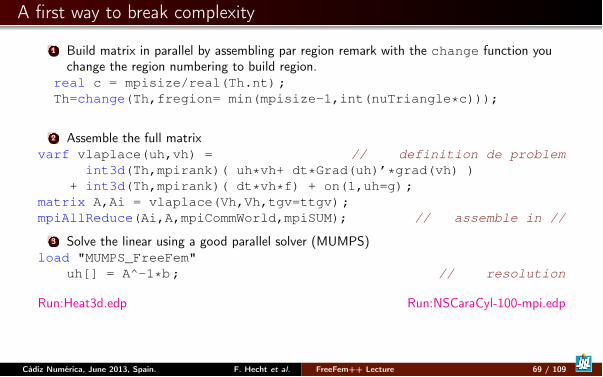
A first way to break complexity
1 Build matrix in parallel by assembling par region remark with the change function youchange the region numbering to build region.
real c = mpisize/real(Th.nt);Th=change(Th,fregion= min(mpisize-1,int(nuTriangle*c)));
2 Assemble the full matrixvarf vlaplace(uh,vh) = // definition de problem
int3d(Th,mpirank)( uh*vh+ dt*Grad(uh)’*grad(vh) )+ int3d(Th,mpirank)( dt*vh*f) + on(1,uh=g);
matrix A,Ai = vlaplace(Vh,Vh,tgv=ttgv);mpiAllReduce(Ai,A,mpiCommWorld,mpiSUM); // assemble in //
3 Solve the linear using a good parallel solver (MUMPS)load "MUMPS_FreeFem"
uh[] = A^-1*b; // resolution
Run:Heat3d.edp Run:NSCaraCyl-100-mpi.edp
Càdiz Numérica, June 2013, Spain. F. Hecht et al. FreeFem++ Lecture 69 / 109

Outline
1 Introduction
2 Tools
3 Academic Examples
4 Numerics Tools
5 Schwarz method with overlapPoisson equation with Schwarz methodTransfer Partparallel GMRESA simple Coarse grid solverNumerical experiment
6 No Linear Problem
7 Technical Remark on freefem++
8 Phase change with Natural Convection
Càdiz Numérica, June 2013, Spain. F. Hecht et al. FreeFem++ Lecture 70 / 109
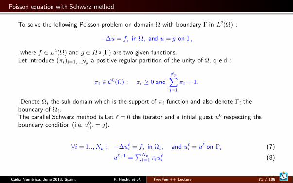
Poisson equation with Schwarz method
To solve the following Poisson problem on domain ⌦ with boundary � in L2(⌦) :
��u = f, in ⌦, and u = g on �,
where f 2 L2(⌦) and g 2 H
12(�) are two given functions.
Let introduce (⇡i)i=1,..,Np a positive regular partition of the unity of ⌦, q-e-d :
⇡i 2 C0(⌦) : ⇡i � 0 and
NpX
i=1
⇡i = 1.
Denote ⌦i the sub domain which is the support of ⇡i function and also denote �i theboundary of ⌦i.The parallel Schwarz method is Let ` = 0 the iterator and a initial guest u0 respecting theboundary condition (i.e. u0
|� = g).
8i = 1.., Np : ��u`i = f, in ⌦i, and u`
i = u` on �i (7)
u`+1=
PNp
i=1 ⇡iu`i (8)
Càdiz Numérica, June 2013, Spain. F. Hecht et al. FreeFem++ Lecture 71 / 109
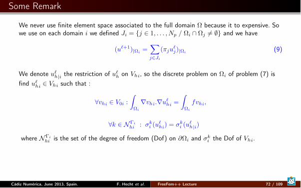
Some Remark
We never use finite element space associated to the full domain ⌦ because it to expensive. Sowe use on each domain i we defined Ji = {j 2 1, . . . , Np / ⌦i \ ⌦j 6= ;} and we have
(u`+1)|⌦i
=
X
j2Ji
(⇡ju`j)|⌦i
(9)
We denote u`h|i the restriction of u`
h on Vhi, so the discrete problem on ⌦i of problem (7) isfind u`
hi 2 Vhi such that :
8vhi 2 V0i :
Z
⌦i
rvhi.ru`hi =
Z
⌦i
fvhi,
8k 2 N�ihi : �k
i (u`hi) = �k
i (u`h|i)
where N�ihi is the set of the degree of freedom (Dof) on @⌦i and �k
i the Dof of Vhi.
Càdiz Numérica, June 2013, Spain. F. Hecht et al. FreeFem++ Lecture 72 / 109
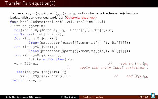
Transfer Part equation(5)
To compute vi = (⇡iui)|⌦i+
Pj2Ji
(⇡juj)|⌦iand can be write the freefem++ function
Update with asynchronous send/recv (Otherwise dead lock).func bool Update(real[int] &ui, real[int] &vi){ int n= jpart.n;
for(int j=0;j<njpart;++j) Usend[j][]=sMj[j]*ui;mpiRequest[int] rq(n*2);for (int j=0;j<n;++j)
Irecv(processor(jpart[j],comm,rq[j ]), Ri[j][]);for (int j=0;j<n;++j)
Isend(processor(jpart[j],comm,rq[j+n]), Si[j][]);for (int j=0;j<n*2;++j)
int k= mpiWaitAny(rq);vi = Pii*ui; // set to (⇡iui)|⌦i
// apply the unity local partition .for(int j=0;j<njpart;++j)
vi += rMj[j]*Vrecv[j][]; // add (⇡juj)|⌦i
return true; }
Càdiz Numérica, June 2013, Spain. F. Hecht et al. FreeFem++ Lecture 73 / 109
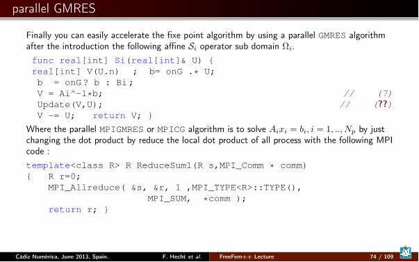
parallel GMRES
Finally you can easily accelerate the fixe point algorithm by using a parallel GMRES algorithmafter the introduction the following affine Si operator sub domain ⌦i.func real[int] Si(real[int]& U) {real[int] V(U.n) ; b= onG .* U;b = onG? b : Bi;V = Ai^-1*b; // (7)Update(V,U); // (??)V -= U; return V; }
Where the parallel MPIGMRES or MPICG algorithm is to solve Aixi = bi, i = 1, .., Np by justchanging the dot product by reduce the local dot product of all process with the following MPIcode :template<class R> R ReduceSum1(R s,MPI_Comm * comm){ R r=0;
MPI_Allreduce( &s, &r, 1 ,MPI_TYPE<R>::TYPE(),MPI_SUM, *comm );
return r; }
Càdiz Numérica, June 2013, Spain. F. Hecht et al. FreeFem++ Lecture 74 / 109
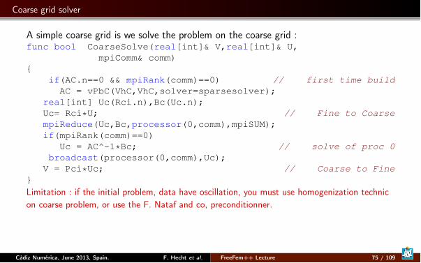
Coarse grid solver
A simple coarse grid is we solve the problem on the coarse grid :func bool CoarseSolve(real[int]& V,real[int]& U,
mpiComm& comm){
if(AC.n==0 && mpiRank(comm)==0) // first time buildAC = vPbC(VhC,VhC,solver=sparsesolver);
real[int] Uc(Rci.n),Bc(Uc.n);Uc= Rci*U; // Fine to CoarsempiReduce(Uc,Bc,processor(0,comm),mpiSUM);if(mpiRank(comm)==0)
Uc = AC^-1*Bc; // solve of proc 0broadcast(processor(0,comm),Uc);
V = Pci*Uc; // Coarse to Fine}Limitation : if the initial problem, data have oscillation, you must use homogenization technicon coarse problem, or use the F. Nataf and co, preconditionner.
Càdiz Numérica, June 2013, Spain. F. Hecht et al. FreeFem++ Lecture 75 / 109
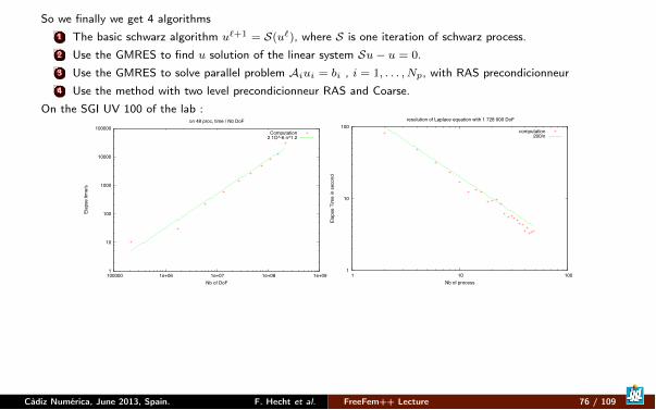
So we finally we get 4 algorithms1 The basic schwarz algorithm u
`+1= S(u`
), where S is one iteration of schwarz process.2 Use the GMRES to find u solution of the linear system Su� u = 0.3 Use the GMRES to solve parallel problem Aiui = bi , i = 1, . . . , Np, with RAS precondicionneur4 Use the method with two level precondicionneur RAS and Coarse.
On the SGI UV 100 of the lab :
1
10
100
1000
10000
100000
100000 1e+06 1e+07 1e+08 1e+09
Elap
se ti
me/
s
Nb of DoF
on 48 proc, time / Nb DoF
Computation2 1O^-6 n^1.2
1
10
100
1 10 100
Elap
se T
ime
in s
econ
d
Nb of process
resolution of Laplace equation with 1 728 000 DoF
computation200/n
Càdiz Numérica, June 2013, Spain. F. Hecht et al. FreeFem++ Lecture 76 / 109
A Parallel Numerical experiment on laptop
We consider first example in an academic situation to solve Poisson Problem on thecube ⌦ =]0, 1[3
��u = 1, in ⌦; u = 0, on @⌦. (10)
With a cartesian meshes Th
n
of ⌦ with 6n3 tetrahedron, the coarse mesh is Th
⇤m
, andm is a divisor of n.We do the validation of the algorithm on a Laptop Intel Core i7 with 4 core at 1.8 Ghzwith 4Go of RAM DDR3 at 1067 Mhz,
Run:DDM-Schwarz-Lap-2dd.edp Run:DDM-Schwarz-Lame-2d.edpRun:DDM-Schwarz-Lame-3d.edp Run:DDM-Schwarz-Stokes-2d.edp
Càdiz Numérica, June 2013, Spain. F. Hecht et al. FreeFem++ Lecture 77 / 109
Outline
1 Introduction
2 Tools
3 Academic Examples
4 Numerics Tools
5 Schwarz method with overlap
6 No Linear ProblemNavier-StokesVariational InequalityGround waterBose Einstein CondensateHyper elasticity equation
7 Technical Remark on freefem++
8 Phase change with Natural Convection
Càdiz Numérica, June 2013, Spain. F. Hecht et al. FreeFem++ Lecture 78 / 109
incompressible Navier-Stokes equation with Newton methods
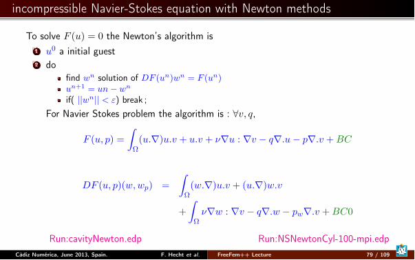
To solve F (u) = 0 the Newton’s algorithm is1 u0 a initial guest2 do
find wn solution of DF (un)wn
= F (un)
un+1= un� wn
if( ||wn|| < ") break ;For Navier Stokes problem the algorithm is : 8v, q,
F (u, p) =
Z
⌦
(u.r)u.v + u.v + ⌫ru : rv � qr.u� pr.v +BC
DF (u, p)(w,wp
) =
Z
⌦
(w.r)u.v + (u.r)w.v
+
Z
⌦
⌫rw : rv � qr.w � pw
r.v +BC0
Run:cavityNewton.edp Run:NSNewtonCyl-100-mpi.edpCàdiz Numérica, June 2013, Spain. F. Hecht et al. FreeFem++ Lecture 79 / 109
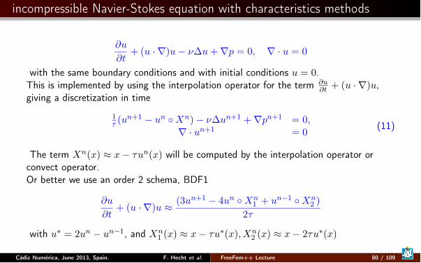
incompressible Navier-Stokes equation with characteristics methods
@u
@t+ (u ·r)u� ⌫�u+rp = 0, r · u = 0
with the same boundary conditions and with initial conditions u = 0.This is implemented by using the interpolation operator for the term @u
@t
+ (u ·r)u,giving a discretization in time
1
⌧
(un+1 � un �Xn
)� ⌫�un+1
+rpn+1
= 0,r · un+1
= 0
(11)
The term Xn
(x) ⇡ x� ⌧un(x) will be computed by the interpolation operator orconvect operator.Or better we use an order 2 schema, BDF1
@u
@t+ (u ·r)u ⇡ (3un+1 � 4un �Xn
1
+ un�1 �Xn
2
)
2⌧
with u⇤ = 2un � un�1, and Xn
1
(x) ⇡ x� ⌧u⇤(x), Xn
2
(x) ⇡ x� 2⌧u⇤(x)
Càdiz Numérica, June 2013, Spain. F. Hecht et al. FreeFem++ Lecture 80 / 109
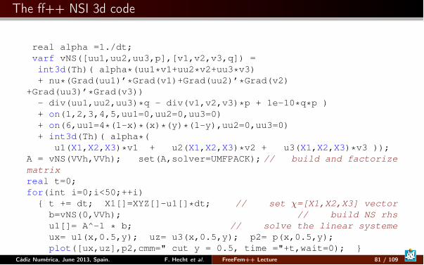
The ff++ NSI 3d code
real alpha =1./dt;varf vNS([uu1,uu2,uu3,p],[v1,v2,v3,q]) =int3d(Th)( alpha*(uu1*v1+uu2*v2+uu3*v3)+ nu*(Grad(uu1)’*Grad(v1)+Grad(uu2)’*Grad(v2)
+Grad(uu3)’*Grad(v3))- div(uu1,uu2,uu3)*q - div(v1,v2,v3)*p + 1e-10*q*p )+ on(1,2,3,4,5,uu1=0,uu2=0,uu3=0)+ on(6,uu1=4*(1-x)*(x)*(y)*(1-y),uu2=0,uu3=0)+ int3d(Th)( alpha*(
u1(X1,X2,X3)*v1 + u2(X1,X2,X3)*v2 + u3(X1,X2,X3)*v3 ));A = vNS(VVh,VVh); set(A,solver=UMFPACK); // build and factorizematrixreal t=0;for(int i=0;i<50;++i){ t += dt; X1[]=XYZ[]-u1[]*dt; // set �=[X1,X2,X3] vector
b=vNS(0,VVh); // build NS rhsu1[]= A^-1 * b; // solve the linear systemeux= u1(x,0.5,y); uz= u3(x,0.5,y); p2= p(x,0.5,y);plot([ux,uz],p2,cmm=" cut y = 0.5, time ="+t,wait=0); }
Run:NSI3d.edpCàdiz Numérica, June 2013, Spain. F. Hecht et al. FreeFem++ Lecture 81 / 109
Variational Inequality
To solve just make a change of variable u = u+ � u�, u > 0 and v = u+ + u� , and weget a classical VI problem on u and and the Poisson on v.
So we can use the algorithm of Primal-Dual Active set strategy as a semi smoothNewton Method HinterMuller , K. Ito, K. Kunisch SIAM J. Optim. V 13, I 3, 2002.
In this case , we just do all implementation by hand in FreeFem++ language
Run:VI-2-membrane-adap.edp
Càdiz Numérica, June 2013, Spain. F. Hecht et al. FreeFem++ Lecture 82 / 109

A Free Boundary problem , (phreatic water)
Let a trapezoidal domain ⌦ defined in FreeFem++ :real L=10; // Widthreal h=2.1; // Left heightreal h1=0.35; // Right heightborder a(t=0,L){x=t;y=0;label=1;}; // impermeable �a
border b(t=0,h1){x=L;y=t;label=2;}; // the source �b
border f(t=L,0){x=t;y=t*(h1-h)/L+h;label=3;}; // �f
border d(t=h,0){x=0;y=t;label=4;}; // Left impermeable �d
int n=10;mesh Th=buildmesh (a(L*n)+b(h1*n)+f(sqrt(L^2+(h-h1)^2)*n)+d(h*n));plot(Th,ps="dTh.eps");
Càdiz Numérica, June 2013, Spain. F. Hecht et al. FreeFem++ Lecture 83 / 109

The initial mesh
The problem is : find p and ⌦ such that :8>>>>>>><
>>>>>>>:
��p = 0 in ⌦
p = y on �
b
@p
@n= 0 on �
d
[ �
a
@p
@n=
q
K
nx
on �
f
(Neumann)
p = y on �
f
(Dirichlet)
where the input water flux is q = 0.02, and K = 0.5. The velocity u of the water isgiven by u = �rp.
Càdiz Numérica, June 2013, Spain. F. Hecht et al. FreeFem++ Lecture 84 / 109
algorithm
We use the following fix point method : (with bad main B.C. Execute freeboundaryPB.edp
) let be, k = 0, ⌦k
= ⌦. First step, we forgot the Neumann BC and we solve theproblem : Find p in V = H1
(⌦
k
), such p = y on �
k
b
et on �
k
f
Z
⌦
k
rprp0 = 0, 8p0 2 V with p0 = 0 on �
k
b
[ �
k
f
With the residual of the Neumann boundary condition we build a domaintransformation F(x, y) = [x, y � v(x)] where v is solution of : v 2 V , such than v = 0
on �
k
a
(bottom)Z
⌦
k
rvrv0 =
Z
�
kf
(
@p
@n� q
Knx
)v0, 8v0 2 V with v0 = 0 sur �k
a
remark : we can use the previous equation to evaluateZ
�
k
@p
@nv0 = �
Z
⌦
k
rprv0
Càdiz Numérica, June 2013, Spain. F. Hecht et al. FreeFem++ Lecture 85 / 109
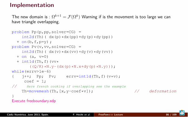
Implementation
The new domain is : ⌦k+1
= F(⌦
k
) Warning if is the movement is too large we canhave triangle overlapping.
problem Pp(p,pp,solver=CG) =int2d(Th)( dx(p)*dx(pp)+dy(p)*dy(pp))
+ on(b,f,p=y);problem Pv(v,vv,solver=CG) =
int2d(Th)( dx(v)*dx(vv)+dy(v)*dy(vv))+ on (a, v=0)+ int1d(Th,f)(vv*
((Q/K)*N.y-(dx(p)*N.x+dy(p)*N.y)));while(errv>1e-6){ j++; Pp; Pv; errv=int1d(Th,f)(v*v);
coef = 1;// Here french cooking if overlapping see the example
Th=movemesh(Th,[x,y-coef*v]); // deformation}Execute freeboundary.edp
Càdiz Numérica, June 2013, Spain. F. Hecht et al. FreeFem++ Lecture 86 / 109
Bose Einstein Condensate
Just a direct use of Ipopt interface (2day of works)The problem is find a complex field u on domain D such that :
u = argmin
||u||=1
Z
D
1
2
|ru|2 + Vtrap
|u|2 + g
2
|u|4� ⌦iu���y
x
�.r�
u
to code that in FreeFem++use
Ipopt interface ( https://projects.coin-or.org/Ipopt)Adaptation de maillage
Run:BEC.edp
Càdiz Numérica, June 2013, Spain. F. Hecht et al. FreeFem++ Lecture 87 / 109
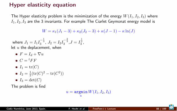
Hyper elasticity equation
The Hyper elasticity problem is the minimization of the energy W (I1
, I2
, I3
) whereI1
, I2
, I3
are the 3 invariants. For example The Ciarlet Geymonat energy model is
W = 1
(J1
� 3) + 2
(J2
� 3) + (J � 1)� ln(J)
where J1
= I1
I� 1
33
, J2
= I2
I� 2
33
,J = I123
,let u the deplacement, when
F = Id
+ru
C =
tFF
I1
= tr(C)
I2
=
1
2
(tr(C)
2 � tr(C2
))
I3
= det(C)
The problem is findu = argmin
u
W (I1
, I2
, I3
)
Càdiz Numérica, June 2013, Spain. F. Hecht et al. FreeFem++ Lecture 88 / 109
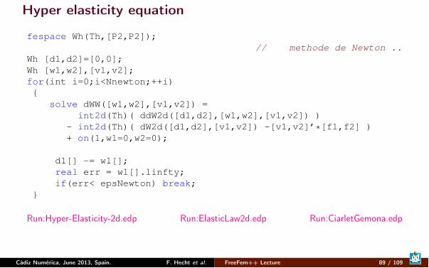
Hyper elasticity equation
fespace Wh(Th,[P2,P2]);// methode de Newton ..
Wh [d1,d2]=[0,0];Wh [w1,w2],[v1,v2];for(int i=0;i<Nnewton;++i){
solve dWW([w1,w2],[v1,v2]) =int2d(Th)( ddW2d([d1,d2],[w1,w2],[v1,v2]) )
- int2d(Th)( dW2d([d1,d2],[v1,v2]) -[v1,v2]’*[f1,f2] )+ on(1,w1=0,w2=0);
d1[] -= w1[];real err = w1[].linfty;if(err< epsNewton) break;
}
Run:Hyper-Elasticity-2d.edp Run:ElasticLaw2d.edp Run:CiarletGemona.edp
Càdiz Numérica, June 2013, Spain. F. Hecht et al. FreeFem++ Lecture 89 / 109
Outline
1 Introduction
2 Tools
3 Academic Examples
4 Numerics Tools
5 Schwarz method with overlap
6 No Linear Problem
7 Technical Remark on freefem++compilation processPluginPlugin to read imagePlugin of link code through a pipeFreeFem++ et C++ type
8 Phase change with Natural Convection
Càdiz Numérica, June 2013, Spain. F. Hecht et al. FreeFem++ Lecture 90 / 109
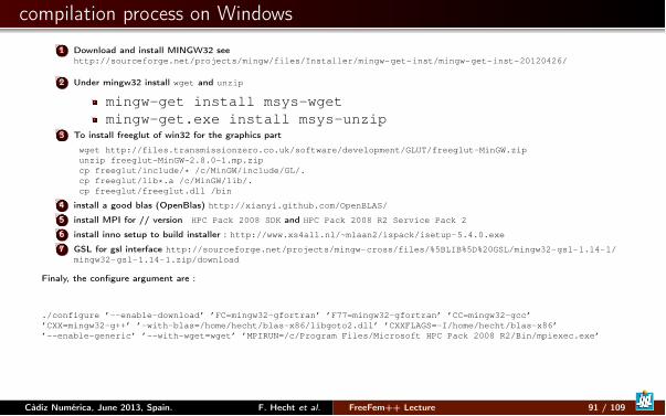
compilation process on Windows1 Download and install MINGW32 see
http://sourceforge.net/projects/mingw/files/Installer/mingw-get-inst/mingw-get-inst-20120426/
2 Under mingw32 install wget and unzip
mingw-get install msys-wgetmingw-get.exe install msys-unzip
3 To install freeglut of win32 for the graphics partwget http://files.transmissionzero.co.uk/software/development/GLUT/freeglut-MinGW.zipunzip freeglut-MinGW-2.8.0-1.mp.zipcp freeglut/include/* /c/MinGW/include/GL/.cp freeglut/lib*.a /c/MinGW/lib/.cp freeglut/freeglut.dll /bin
4 install a good blas (OpenBlas) http://xianyi.github.com/OpenBLAS/
5 install MPI for // version HPC Pack 2008 SDK and HPC Pack 2008 R2 Service Pack 2
6 install inno setup to build installer : http://www.xs4all.nl/~mlaan2/ispack/isetup-5.4.0.exe7 GSL for gsl interface http://sourceforge.net/projects/mingw-cross/files/%5BLIB%5D%20GSL/mingw32-gsl-1.14-1/
mingw32-gsl-1.14-1.zip/download
Finaly, the configure argument are :
./configure ’--enable-download’ ’FC=mingw32-gfortran’ ’F77=mingw32-gfortran’ ’CC=mingw32-gcc’’CXX=mingw32-g++’ ’-with-blas=/home/hecht/blas-x86/libgoto2.dll’ ’CXXFLAGS=-I/home/hecht/blas-x86’’--enable-generic’ ’--with-wget=wget’ ’MPIRUN=/c/Program Files/Microsoft HPC Pack 2008 R2/Bin/mpiexec.exe’
Càdiz Numérica, June 2013, Spain. F. Hecht et al. FreeFem++ Lecture 91 / 109
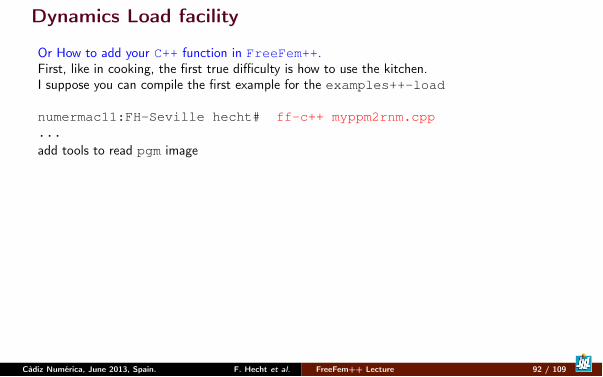
Dynamics Load facility
Or How to add your C++ function in FreeFem++.First, like in cooking, the first true difficulty is how to use the kitchen.I suppose you can compile the first example for the examples++-load
numermac11:FH-Seville hecht# ff-c++ myppm2rnm.cpp...add tools to read pgm image
Càdiz Numérica, June 2013, Spain. F. Hecht et al. FreeFem++ Lecture 92 / 109
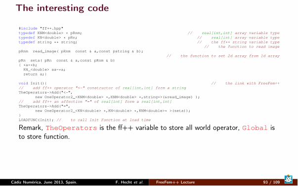
The interesting code
#include "ff++.hpp"typedef KNM<double> * pRnm; // real[int,int] array variable typetypedef KN<double> * pRn; // real[int] array variable typetypedef string ** string; // the ff++ string variable type
// the function to read imagepRnm read_image( pRnm const & a,const pstring & b);
// the function to set 2d array from 1d arraypRn seta( pRn const & a,const pRnm & b){ *a=*b;
KN_<double> aa=*a;return a;}
void Init(){ // the link with FreeFem++// add ff++ operator "<-" constructor of real[int,int] form a stringTheOperators->Add("<-",
new OneOperator2_<KNM<double> *,KNM<double> *,string*>(&read_image) );// add ff++ an affection "=" of real[int] form a real[int,int]TheOperators->Add("=",
new OneOperator2_<KN<double> *,KN<double> *,KNM<double>* >(seta));}LOADFUNC(Init); // to call Init Function at load time
Remark, TheOperators is the ff++ variable to store all world operator, Global isto store function.
Càdiz Numérica, June 2013, Spain. F. Hecht et al. FreeFem++ Lecture 93 / 109
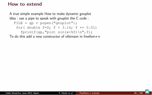
How to extend
A true simple example How to make dynamic gnuplotIdea : use a pipe to speak with gnuplot the C code :FILE * gp = popen("gnuplot");for( double f=0; f < 3.14; f += 0.01)fprintf(gp,"plot sin(x+%f)\n",f);
To do this add a new constructor of ofstream in freefem++
Càdiz Numérica, June 2013, Spain. F. Hecht et al. FreeFem++ Lecture 94 / 109
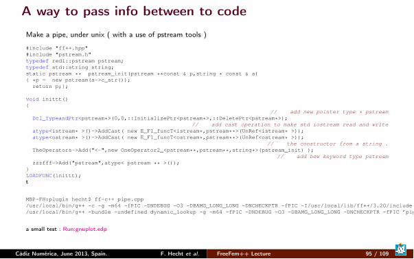
A way to pass info between to code
Make a pipe, under unix ( with a use of pstream tools )
#include "ff++.hpp"#include "pstream.h"typedef redi::pstream pstream;typedef std::string string;static pstream ** pstream_init(pstream **const & p,string * const & a){ *p = new pstream(a->c_str());
return p;};
void inittt(){
// add new pointer type * pstreamDcl_TypeandPtr<pstream*>(0,0,::InitializePtr<pstream*>,::DeletePtr<pstream*>);
// add cast operation to make std iostream read and writeatype<istream* >()->AddCast( new E_F1_funcT<istream*,pstream**>(UnRef<istream* >));atype<ostream* >()->AddCast( new E_F1_funcT<ostream*,pstream**>(UnRef<ostream* >));
// the constructor from a string .TheOperators->Add("<-",new OneOperator2_<pstream**,pstream**,string*>(pstream_init) );
// add new keyword type pstreamzzzfff->Add("pstream",atype< pstream ** >());
}LOADFUNC(inittt);t
MBP-FH:plugin hecht$ ff-c++ pipe.cpp/usr/local/bin/g++ -c -g -m64 -fPIC -DNDEBUG -O3 -DBAMG_LONG_LONG -DNCHECKPTR -fPIC -I/usr/local/lib/ff++/3.20/include ’pipe.cpp’/usr/local/bin/g++ -bundle -undefined dynamic_lookup -g -m64 -fPIC -DNDEBUG -O3 -DBAMG_LONG_LONG -DNCHECKPTR -fPIC ’pipe.o’ -o pipe.dylib
a small test : Run:gnuplot.edp
Càdiz Numérica, June 2013, Spain. F. Hecht et al. FreeFem++ Lecture 95 / 109
FreeFem++ et C++ type
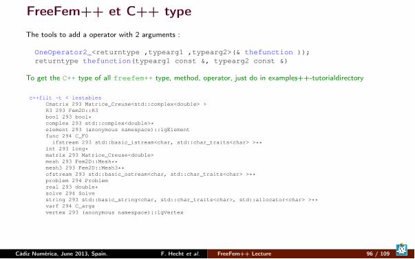
The tools to add a operator with 2 arguments :
OneOperator2_<returntype ,typearg1 ,typearg2>(& thefunction ));returntype thefunction(typearg1 const &, typearg2 const &)
To get the C++ type of all freefem++ type, method, operator, just do in examples++-tutorialdirectory
c++filt -t < lestablesCmatrix 293 Matrice_Creuse<std::complex<double> >R3 293 Fem2D::R3bool 293 bool*complex 293 std::complex<double>*element 293 (anonymous namespace)::lgElementfunc 294 C_F0
ifstream 293 std::basic_istream<char, std::char_traits<char> >**int 293 long*matrix 293 Matrice_Creuse<double>mesh 293 Fem2D::Mesh**mesh3 293 Fem2D::Mesh3**ofstream 293 std::basic_ostream<char, std::char_traits<char> >**problem 294 Problemreal 293 double*solve 294 Solvestring 293 std::basic_string<char, std::char_traits<char>, std::allocator<char> >**varf 294 C_argsvertex 293 (anonymous namespace)::lgVertex
Càdiz Numérica, June 2013, Spain. F. Hecht et al. FreeFem++ Lecture 96 / 109
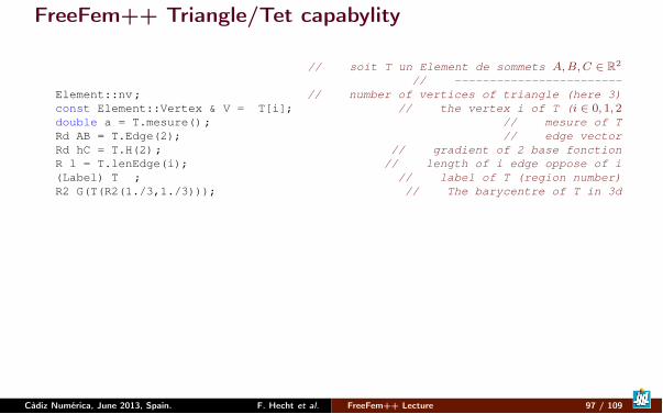
FreeFem++ Triangle/Tet capabylity
// soit T un Element de sommets A,B,C 2 R2
// ------------------------Element::nv; // number of vertices of triangle (here 3)const Element::Vertex & V = T[i]; // the vertex i of T (i 2 0, 1, 2
double a = T.mesure(); // mesure of TRd AB = T.Edge(2); // edge vectorRd hC = T.H(2); // gradient of 2 base fonctionR l = T.lenEdge(i); // length of i edge oppose of i(Label) T ; // label of T (region number)R2 G(T(R2(1./3,1./3))); // The barycentre of T in 3d
Càdiz Numérica, June 2013, Spain. F. Hecht et al. FreeFem++ Lecture 97 / 109

FreeFem++ Mesh/Mesh3 capabylity
Mesh Th("filename"); // read the mesh in "filename"Th.nt; // number of element (triangle or tet)Th.nv; // number of verticesTh.neb or Th.nbe; // numbe rof border element (2d) or(3d)Th.area; // area of the domain (2d)Th.peri; // length of the bordertypedef Mesh::Rd Rd; // R2 or R3Mesh2::Element & K = Th[i]; // triangle i , int i2 [0, nt[
Rd A=K[0]; // coor of vertex 0 of triangle KRd G=K(R2(1./3,1./3)): // the barycentre de K.Rd DLambda[3];K.Gradlambda(DLambda); // compute the 3 r�
Ki for i = 0, 1, 2
Mesh::Vertex & V = Th(j); // vertex j , int j2 [0, nv[
Mesh::BorderElement & BE=th.be(l); // border element l2 [0, nbe[
Rd B=BE[1]; // coord of vertex 1 on Seg BERd M=BE(0.5); // middle of BE.int j = Th(i,k); // global number of vertex k2 [0, 3[ of tria. i2 [0, nt[
Mesh::Vertex & W=Th[i][k]; // vertex k2 [0, 3[ of triangle i2 [0, nt[
int ii = Th(K); // number of triangle Kint jj = Th(V); // number of triangle Vint ll = Th(BE); // number of Seg de bord BEassert( i == ii && j == jj); // check.
Càdiz Numérica, June 2013, Spain. F. Hecht et al. FreeFem++ Lecture 98 / 109
Outline
1 Introduction
2 Tools
3 Academic Examples
4 Numerics Tools
5 Schwarz method with overlap
6 No Linear Problem
7 Technical Remark on freefem++
8 Phase change with Natural ConvectionCàdiz Numérica, June 2013, Spain. F. Hecht et al. FreeFem++ Lecture 99 / 109
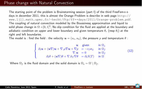
Phase change with Natural Convection
The starting point of the problem is Brainstorming session (part I) of the third FreeFem++days in december 2011, this is almost the Orange Problem is describe in web page http://www.ljll.math.upmc.fr/~hecht/ftp/ff++days/2011/Orange-problem.pdf.The coupling of natural convection modeled by the Boussinesq approximation and liquid tosolid phase change in ⌦ =]0, 1[2, No slip condition for the fluid are applied at the boundary andadiabatic condition on upper and lower boundary and given temperature ✓r (resp ✓l) at theright and left boundaries.The model is : find the field : the velocity u = (u1, u2), the pressure p and temperature ✓ :
8>><
>>:
u given in ⌦s
@tu+ (ur)u+r.µru+rp = �cTe2 in ⌦f
r.u = 0 in ⌦f
@t✓ + (ur)✓ +r.kTr✓ = @tS(T ) in ⌦
(12)
Where ⌦f is the fluid domain and the solid domain is ⌦s = ⌦ \ ⌦f .
Càdiz Numérica, June 2013, Spain. F. Hecht et al. FreeFem++ Lecture 100 / 109
Phase change with Natural Convection
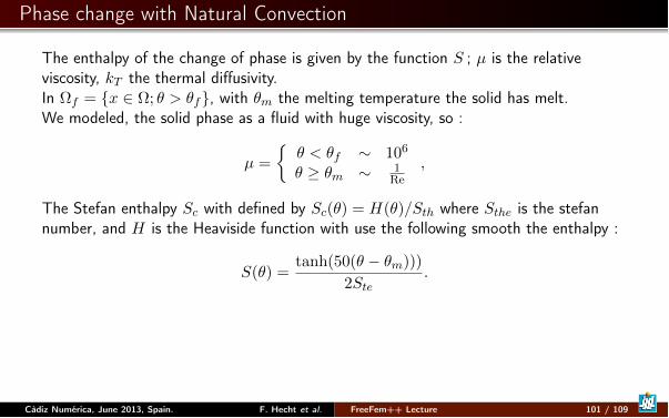
The enthalpy of the change of phase is given by the function S ; µ is the relativeviscosity, k
T
the thermal diffusivity.In ⌦
f
= {x 2 ⌦; ✓ > ✓f
}, with ✓m
the melting temperature the solid has melt.We modeled, the solid phase as a fluid with huge viscosity, so :
µ =
⇢✓ < ✓
f
⇠ 10
6
✓ � ✓m
⇠ 1
Re
,
The Stefan enthalpy Sc
with defined by Sc
(✓) = H(✓)/Sth
where Sthe
is the stefannumber, and H is the Heaviside function with use the following smooth the enthalpy :
S(✓) =tanh(50(✓ � ✓
m
)))
2Ste
.
Càdiz Numérica, June 2013, Spain. F. Hecht et al. FreeFem++ Lecture 101 / 109
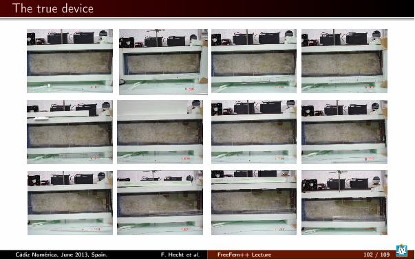
The true device
12 Etude MCPAM °52C
Càdiz Numérica, June 2013, Spain. F. Hecht et al. FreeFem++ Lecture 102 / 109
the Algorithm
We apply a fixed point algorithm for the phase change part (the domain ⌦
f
is fixed ateach iteration) and a full no-linear Euler implicit scheme with a fixed domain for therest. We use a Newton method to solve the non-linearity.
if we don’t make mesh adaptation, the Newton method do not convergeif we use explicit method diverge too,if we implicit the dependance in ⌦
s
the method also diverge.
This is a really difficult problem.
Càdiz Numérica, June 2013, Spain. F. Hecht et al. FreeFem++ Lecture 103 / 109
the Algorithm, implementation
The finite element space to approximate u1, u2, p, ✓ is defined by
fespace Wh(Th,[P2,P2,P1,P1]);
We do mesh adaptation a each time step, with the following code :
Ph ph = S(T), pph=S(Tp);Th= adaptmesh(Th,T,Tp,ph,pph,[u1,u2],err=errh,
hmax=hmax,hmin=hmax/100,ratio = 1.2);
This mean, we adapt with all variable plus the 2 melting phase a time n+ 1 and n andwe smooth the metric with a ratio of 1.2 to account for the movement of the meltingfront.
Càdiz Numérica, June 2013, Spain. F. Hecht et al. FreeFem++ Lecture 104 / 109
The Newton loop
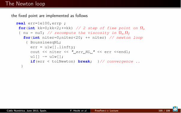
the fixed point are implemented as follows
real err=1e100,errp ;for(int kk=0;kk<2;++kk) // 2 step of fixe point on ⌦s
{ nu = nuT; // recompute the viscosity in ⌦s,⌦f
for(int niter=0;niter<20; ++ niter) // newton loop{ BoussinesqNL;
err = u1w[].linfty;cout << niter << " err NL " << err <<endl;u1[] -= u1w[];if(err < tolNewton) break; }// convergence ..
}
Càdiz Numérica, June 2013, Spain. F. Hecht et al. FreeFem++ Lecture 105 / 109
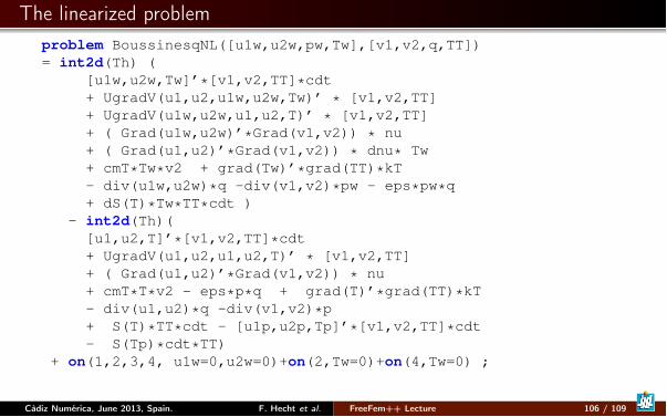
The linearized problemproblem BoussinesqNL([u1w,u2w,pw,Tw],[v1,v2,q,TT])= int2d(Th) (
[u1w,u2w,Tw]’*[v1,v2,TT]*cdt+ UgradV(u1,u2,u1w,u2w,Tw)’ * [v1,v2,TT]+ UgradV(u1w,u2w,u1,u2,T)’ * [v1,v2,TT]+ ( Grad(u1w,u2w)’*Grad(v1,v2)) * nu+ ( Grad(u1,u2)’*Grad(v1,v2)) * dnu* Tw+ cmT*Tw*v2 + grad(Tw)’*grad(TT)*kT- div(u1w,u2w)*q -div(v1,v2)*pw - eps*pw*q+ dS(T)*Tw*TT*cdt )
- int2d(Th)([u1,u2,T]’*[v1,v2,TT]*cdt+ UgradV(u1,u2,u1,u2,T)’ * [v1,v2,TT]+ ( Grad(u1,u2)’*Grad(v1,v2)) * nu+ cmT*T*v2 - eps*p*q + grad(T)’*grad(TT)*kT- div(u1,u2)*q -div(v1,v2)*p+ S(T)*TT*cdt - [u1p,u2p,Tp]’*[v1,v2,TT]*cdt- S(Tp)*cdt*TT)
+ on(1,2,3,4, u1w=0,u2w=0)+on(2,Tw=0)+on(4,Tw=0) ;
Càdiz Numérica, June 2013, Spain. F. Hecht et al. FreeFem++ Lecture 106 / 109
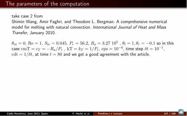
The parameters of the computation
take case 2 fromShimin Wang, Amir Faghri, and Theodore L. Bergman. A comprehensive numericalmodel for melting with natural convection. International Journal of Heat and MassTransfer, January 2010.
✓m
= 0, Re = 1, Ste
= 0.045, Pr
= 56.2, Ra
= 3.27 10
5 , ✓l
= 1, ✓r
= �0.1 so in thiscase cmT = c
T
= �Ra
/Pr
, kT = kT
= 1/Pr
, eps = 10
�6, time step �t = 10
�1,cdt = 1/�t, at time t = 80 and we get a good agreement with the article.
Càdiz Numérica, June 2013, Spain. F. Hecht et al. FreeFem++ Lecture 107 / 109
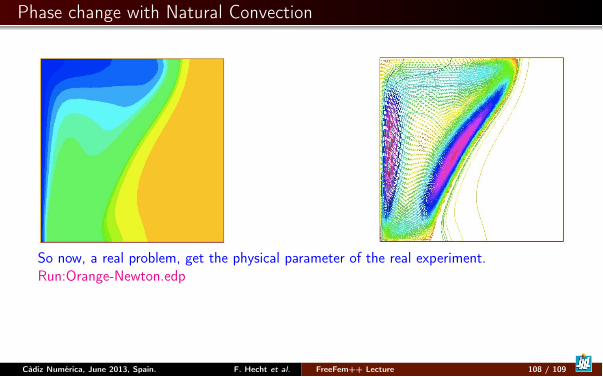
Phase change with Natural Convection
So now, a real problem, get the physical parameter of the real experiment.Run:Orange-Newton.edp
Càdiz Numérica, June 2013, Spain. F. Hecht et al. FreeFem++ Lecture 108 / 109
Conclusion/Future
Freefem++ v3.23 isvery good tool to solve non standard PDE in 2D/3Dto try new domain decomposition domain algorithm
The the future we try to do :Build more graphic with VTK, paraview , ... (in progress)Add Finite volume facility for hyperbolic PDE (just begin C.F. FreeVol Projet)3d anisotrope mesh adaptationautomate the parallel tool
Thank for you attention.
Càdiz Numérica, June 2013, Spain. F. Hecht et al. FreeFem++ Lecture 109 / 109


![Introduction to FreeFem++-cs - UNAMmmc.geofisica.unam.mx/acl/edp/Ejemplitos/FreeFEM/FreeFemIntroduction.pdfin HTML from the web [3]. through other documents in the Manuals section](https://img.pdfslide.us/doc/110x75/5e87cbdc3dff681b76760740/introduction-to-freefem-cs-in-html-from-the-web-3-through-other-documents.jpg)