APPROXIMATION THEORY AND APPROX-

IMATION PRACTICE

Nick Trefethen, TU Berlin, February 2010

Contents

• 1. Introduction• 2. Chebyshev points and interpolants• 3. Chebyshev polynomials and series• 4. Interpolants, truncations, and aliasing• 5. Barycentric interpolation formula• 6. The Weierstrass Approximation Theorem• 7. Convergence for differentiable functions• 8. Convergence for analytic functions• 9. The Gibbs phenomenon• 10. Best approximation• 11. Equispaced points, Runge phenomenon• 12. Discussion of high-order polynomial interpolation• 13. Lebesgue constants• 14. Best and near-best• 15. Legendre points and polynomials• 16. Clenshaw–Curtis and Gauss quadrature• 17. Polynomial CF approximation• 18. Polynomial roots, colleague matrices• References

1. Introduction

Welcome to a beautiful subject! — the constructive approximation of functions.And welcome to a rather unusual book.

Approximation theory is a well-established field, and our aim is to teach yousome of its most important ideas and results. The style of this book, however,is quite different from what you will find elsewhere. Everything is illustratedcomputationally with the help of the chebfun software package in Matlab, fromChebyshev interpolants to Lebesgue constants, from the Weierstrass Approxi-mation Theorem to the Remez algorithm. Everything is practical and fast, sowe will routinely compute polynomial interpolants or Gauss quadrature nodesand weights for tens of thousands of points. In fact, each chapter of this bookis a single Matlab M-file, and the book has been produced by executing thesefiles with Matlab’s “publish” facility. The chapters come from M-files calledchap1.m, chap2.m, . . . , and you can download them and use them as templatesto be modified for explorations of your own.

1

Beginners are welcome, and so are experts, who will find familiar topics ap-proached from new angles and familiar conclusions turned on their heads. In-deed, the field of approximation theory came of age in an era of polynomialsof degrees perhaps O(10). Now that O(1000) is easy and O(1000000) is nothard, different questions come to the fore. In particular we shall see that “best”approximants are hardly better than “near-best,” though they are much harderto compute.

This is a book about approximation, not about chebfun, and for the most partwe shall use chebfun tools without explaining them. A brief introduction tochebfun is given in the Appendix, and for much more information, see the Guideand the download page at

http://www.maths.ox.ac.uk/chebfun/

In the course of the book we shall use chebfun overloads of the following Matlabfunctions, among others:

CUMSUM, DIFF, INTERP1, NORM, POLY, POLYFIT, SPLINE

as well as the additional chebfun commands

CF, CHEBPADE, CHEBPOLY, CHEBPOLYPLOT, CHEBPOLYVAL,

CHEBPTS, LEBESGUE, LEGPOLY, LEGPTS, RATINTERP, REMEZ.

There are quite a number of excellent books on approximation theory. Threeclassics are [Cheney 1966], [Davis 1963], and [Meinardus 1967], and a morerecent computationally oriented classic is [Powell 1981].

A good deal of our emphasis will be on ideas related to Chebyshev points andpolynomials, whose roots go back a century or more to mathematicians in-cluding Chebyshev (1821–1894), Zolotarev (1847–1878), de la Vallee Poussin(1866–1962), Bernstein (1880–1968), and Dunham Jackson (1888–1946). In thecomputer era, some of the early figures who developed “Chebyshev technol-ogy,” in approximately chronological order, were Lanczos, Clenshaw, Specht,Good, Fox, Elliott, Mason, and Orszag. Two books on Chebyshev polynomialsare [Rivlin 1990] and [Mason & Handscomb 2003]. One reason we emphasizeChebyshev technology so much is that in practice, for working with functions onintervals, these methods are unbeatable. For example, we shall see in Chapter14 that the difference in approximation power between Chebyshev and “opti-mal” interpolation points is utterly negligible. Another reason is that if youknow the Chebyshev material solidly, this is the best possible foundation forwork on other approximation ideas.

Our mathematical style is conversational, but that doesn’t mean the material iselementary. The book aims to be more readable than most, and the numerical

2

experiments help achieve this. At the same time, theorems are stated and proofsare given, often rather terse, without all the details spelled out. It is assumedthat reader is comfortable with rigorous mathematical arguments and familiarwith ideas like continuous functions on compact sets, Lipschitz continuity, con-tour integrals in the complex plane, and norms of matrices and operators. If youare a student, I hope you are an advanced undergraduate or graduate who hastaken courses in numerical analysis and complex analysis. If you are a seasonedmathematician, I hope you are also a Matlab user!

This book was produced using publish in LaTeX mode: thus this chapter, forexample, can be generated with the command publish(’chap1’,’latex’). Toachieve the desired layout we begin by setting a few default parameters:

set(0,’defaultfigureposition’,[380 320 540 200],...

’defaultaxeslinewidth’,0.9,’defaultaxesfontsize’,8,...

’defaultlinelinewidth’,1.1,’defaultpatchlinewidth’,1.1,...

’defaultlinemarkersize’,15), format compact, format long

chebfunpref(’factory’); clear all, x = chebfun(’x’,[-1 1]);

To make the chapters independently executable, it is necessary to include thesestatements at the beginning of each. This would lead to a clutter of text, soinstead, at the beginning of each chapter we execute the command

ATAPformats

which calls an M-file containing the code above. This isn’t beautiful, but itworks. For convenience, ATAPformats is included in the standard distribution ofthe chebfun package. (For the actual production of the printed book, publishwas executed not chapter-by-chapter but on a big file concatenating all thechapters, and a few tweaks were made to the resulting LaTeX file.)

The Lagrange interpolation formula was discovered by Waring, the Gibbs phe-nomenon was discovered by Wilbraham, and the Runge phenomenon was firstglimpsed, if perhaps not very clearly, by Meray. These are just some of theinstances of Stigler’s Law in approximation theory, and the reader will see myinterest in history in the references section, where original sources are usuallygiven and the entries stretch back several centuries, each with an editorial com-ment attached. Often the originals are surprisingly readable and insightful, andin any case, it seems especially important to pay heed to original sources in abook like this that aims to reexamine material that has grown too standardizedin the textbooks. Another reason for looking at original sources is that in thelast few years, thanks to digitization of journals, it has become far easier totrack them down than it used to be, though there are always difficult specialcases like [Wilbraham 1848], which I finally found in an elegant leather-boundvolume in the Balliol College library.

3

Perhaps I may add a further personal comment. As an undergraduate andgraduate student in the late 1970s and early 1980s, one of my main interestswas approximation theory. I regarded this subject as the foundation of mywider field of numerical analysis — but as the years passed, it came to seemdry and academic, and I moved into other areas. Now times have changed,computers have changed, and my perceptions have changed. I now again regardapproximation theory as exceedingly close to computing, and this view hasbeen reinforced by new developments including wavelets, radial basis functions,and compressed sensing. The topics discussed here are a bit more classicalthan those: the foundations of univariate approximation theory. As I hope thisbook will show, there is scarcely an idea in this area that can’t be illustratedcompellingly in a few lines of chebfun code, and as I first imagined around 1975,anyone who wants to be expert at numerical computation really does need toknow this material.

Exercise 1.1. Chebfun download. Download the current version of the cheb-fun package from www.maths.ox.ac.uk/chebfun/ and install it in your Matlabpath as instructed at the web site. Execute the command chebtest to makesure things are working, and note the time taken. Execute chebtest again andsee how much speedup there is now that various files have been brought intomemory.

Exercise 1.2. The publish command. Execute help publish

and doc publish in Matlab to learn the basics of how the publish

command works. Then download chap1.m and chap2.m fromwww.maths.ox.ac.uk/chebfun/ and publish them in HTML with a Mat-lab command like open(publish(’cheb.1’)). Now publish them again withpublish(’chap2’,’latex’) followed by appropriate LaTeX commands. (Youwill probably find that chap1.tex and chap2.tex appear in a subdirectory onyour computer labeled html.) If you are a student taking in a course for whichyou are expected to turn in writeups of the exercises, then you could hardly dobetter than to make it a habit of producing them with publish.

2. Chebyshev points and interpolants

As always we begin a chapter by setting the default formats:

ATAPformats

Any interval [a, b] can be scaled to [−1, 1], so most of the time, we shall justtalk about [−1, 1].

Let n be a positive integer:

4

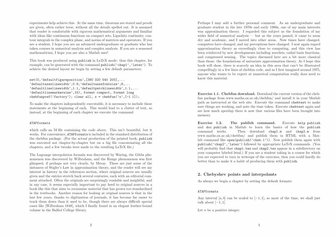
n = 16;

Consider n + 1 equally spaced angles {θj} from 0 to π:

tt = linspace(0,pi,n+1);

We can think of these as the arguments of n+1 points {zj} on the upper half ofthe unit circle in the complex plane. These are the (2n)th roots of unity lyingin the closed upper half-plane:

zz = exp(1i*tt);

hold off, plot(zz,’.-k’), axis equal, ylim([0 1.1])

title(’Equispaced points on the unit circle’)

−1 −0.5 0 0.5 10

0.2

0.4

0.6

0.8

1

Equispaced points on the unit circle

The Chebyshev points associated with the parameter n are the real parts ofthese points,

xj = Re zj =1

2(zj + z−1

j ), 0 ≤ j ≤ n :

xx = real(zz);

Some authors use the terms Chebyshev-Lobatto points, Chebyshev ex-

treme points, or Chebyshev points of the second kind, but as these arethe points most often used in practical computation, we shall just say Chebyshevpoints.

Another way to define the Chebyshev points is in terms of the original angles:

xj = cos(jπ/n), 0 ≤ j ≤ n,

xx = cos(tt);

5

There is also an equivalent chebfun command chebpts:

xx = chebpts(n+1);

Actually this result isn’t exactly equivalent, as the ordering is left-to-right ratherthan right-to-left.

Let us add the Chebyshev points to the plot:

hold on, plot(xx,0*xx,’.r’), title(’Chebyshev points’)

−1 −0.5 0 0.5 10

0.2

0.4

0.6

0.8

1

Chebyshev points

They cluster near 1 and −1, with the average spacing as n → ∞ being given bya density function with square root singularities at both ends (Exercise 2.2).

Let {fj}, 0 ≤ j ≤ n, be a set of numbers, which may or may not come fromsampling a function f(x) at the Chebyshev points. Then there exists a uniquepolynomial p of degree n that interpolates these data, i.e., p(xj) = fj for eachj. When we say “of degree n,” we mean of degree less than or equal to n.As we trust the reader already knows, the existence and uniqueness of poly-nomial interpolants applies for any distinct set of interpolation points. In thiscase of special interest involving Chebyshev points, we call the polynomial theChebyshev interpolant.

Polynomial interpolants through equally spaced points have terrible properties,and we shall explore this effect in Chapters 11–13. Polynomial interpolantsthrough Chebyshev points, however, are excellent. It is the clustering nearthe ends of the interval that makes the difference, and other sets of pointswith similar clustering, like Legendre points (Chapter 15), have similarly goodbehavior. The explanation of this fact has a lot to do with potential theory[Ransford 1995, Smirnov & Lebedev 1968, Walsh 1969], but we shall not go intothat in this book.

The chebfun system is built on Chebyshev interpolants. For example, here is acertain step function:

6

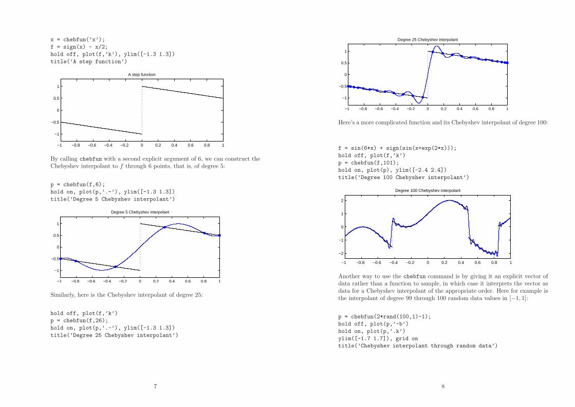
x = chebfun(’x’);

f = sign(x) - x/2;

hold off, plot(f,’k’), ylim([-1.3 1.3])

title(’A step function’)

−1 −0.8 −0.6 −0.4 −0.2 0 0.2 0.4 0.6 0.8 1

−1

−0.5

0

0.5

1

A step function

By calling chebfun with a second explicit argument of 6, we can construct theChebyshev interpolant to f through 6 points, that is, of degree 5:

p = chebfun(f,6);

hold on, plot(p,’.-’), ylim([-1.3 1.3])

title(’Degree 5 Chebyshev interpolant’)

−1 −0.8 −0.6 −0.4 −0.2 0 0.2 0.4 0.6 0.8 1

−1

−0.5

0

0.5

1

Degree 5 Chebyshev interpolant

Similarly, here is the Chebyshev interpolant of degree 25:

hold off, plot(f,’k’)

p = chebfun(f,26);

hold on, plot(p,’.-’), ylim([-1.3 1.3])

title(’Degree 25 Chebyshev interpolant’)

7

−1 −0.8 −0.6 −0.4 −0.2 0 0.2 0.4 0.6 0.8 1

−1

−0.5

0

0.5

1

Degree 25 Chebyshev interpolant

Here’s a more complicated function and its Chebyshev interpolant of degree 100:

f = sin(6*x) + sign(sin(x+exp(2*x)));

hold off, plot(f,’k’)

p = chebfun(f,101);

hold on, plot(p), ylim([-2.4 2.4])

title(’Degree 100 Chebyshev interpolant’)

−1 −0.8 −0.6 −0.4 −0.2 0 0.2 0.4 0.6 0.8 1

−2

−1

0

1

2

Degree 100 Chebyshev interpolant

Another way to use the chebfun command is by giving it an explicit vector ofdata rather than a function to sample, in which case it interprets the vector asdata for a Chebyshev interpolant of the appropriate order. Here for example isthe interpolant of degree 99 through 100 random data values in [−1, 1]:

p = chebfun(2*rand(100,1)-1);

hold off, plot(p,’-b’)

hold on, plot(p,’.k’)

ylim([-1.7 1.7]), grid on

title(’Chebyshev interpolant through random data’)

8

−1 −0.8 −0.6 −0.4 −0.2 0 0.2 0.4 0.6 0.8 1

−1.5

−1

−0.5

0

0.5

1

1.5

Chebyshev interpolant through random data

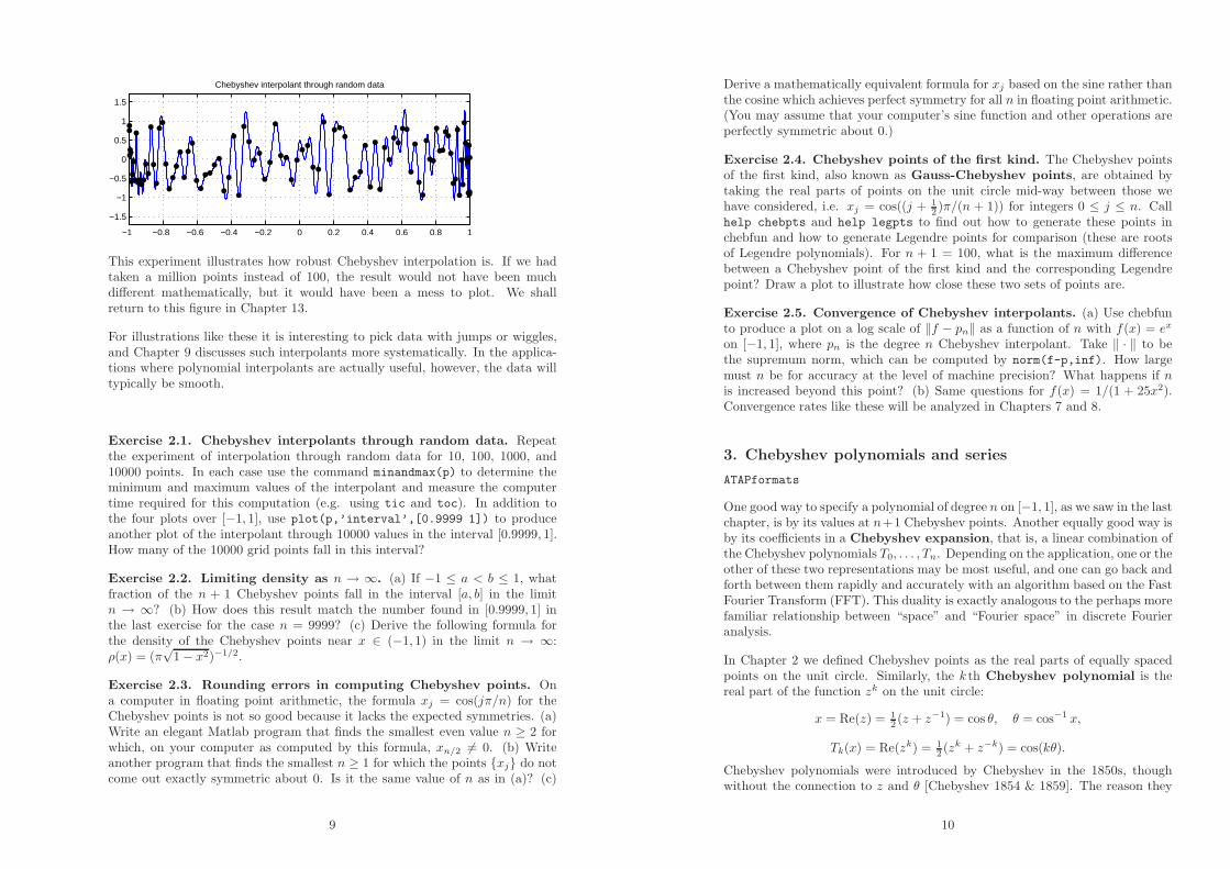
This experiment illustrates how robust Chebyshev interpolation is. If we hadtaken a million points instead of 100, the result would not have been muchdifferent mathematically, but it would have been a mess to plot. We shallreturn to this figure in Chapter 13.

For illustrations like these it is interesting to pick data with jumps or wiggles,and Chapter 9 discusses such interpolants more systematically. In the applica-tions where polynomial interpolants are actually useful, however, the data willtypically be smooth.

Exercise 2.1. Chebyshev interpolants through random data. Repeatthe experiment of interpolation through random data for 10, 100, 1000, and10000 points. In each case use the command minandmax(p) to determine theminimum and maximum values of the interpolant and measure the computertime required for this computation (e.g. using tic and toc). In addition tothe four plots over [−1, 1], use plot(p,’interval’,[0.9999 1]) to produceanother plot of the interpolant through 10000 values in the interval [0.9999, 1].How many of the 10000 grid points fall in this interval?

Exercise 2.2. Limiting density as n → ∞. (a) If −1 ≤ a < b ≤ 1, whatfraction of the n + 1 Chebyshev points fall in the interval [a, b] in the limitn → ∞? (b) How does this result match the number found in [0.9999, 1] inthe last exercise for the case n = 9999? (c) Derive the following formula forthe density of the Chebyshev points near x ∈ (−1, 1) in the limit n → ∞:ρ(x) = (π

√1 − x2)−1/2.

Exercise 2.3. Rounding errors in computing Chebyshev points. Ona computer in floating point arithmetic, the formula xj = cos(jπ/n) for theChebyshev points is not so good because it lacks the expected symmetries. (a)Write an elegant Matlab program that finds the smallest even value n ≥ 2 forwhich, on your computer as computed by this formula, xn/2 6= 0. (b) Writeanother program that finds the smallest n ≥ 1 for which the points {xj} do notcome out exactly symmetric about 0. Is it the same value of n as in (a)? (c)

9

Derive a mathematically equivalent formula for xj based on the sine rather thanthe cosine which achieves perfect symmetry for all n in floating point arithmetic.(You may assume that your computer’s sine function and other operations areperfectly symmetric about 0.)

Exercise 2.4. Chebyshev points of the first kind. The Chebyshev pointsof the first kind, also known as Gauss-Chebyshev points, are obtained bytaking the real parts of points on the unit circle mid-way between those wehave considered, i.e. xj = cos((j + 1

2 )π/(n + 1)) for integers 0 ≤ j ≤ n. Callhelp chebpts and help legpts to find out how to generate these points inchebfun and how to generate Legendre points for comparison (these are rootsof Legendre polynomials). For n + 1 = 100, what is the maximum differencebetween a Chebyshev point of the first kind and the corresponding Legendrepoint? Draw a plot to illustrate how close these two sets of points are.

Exercise 2.5. Convergence of Chebyshev interpolants. (a) Use chebfunto produce a plot on a log scale of ‖f − pn‖ as a function of n with f(x) = ex

on [−1, 1], where pn is the degree n Chebyshev interpolant. Take ‖ · ‖ to bethe supremum norm, which can be computed by norm(f-p,inf). How largemust n be for accuracy at the level of machine precision? What happens if nis increased beyond this point? (b) Same questions for f(x) = 1/(1 + 25x2).Convergence rates like these will be analyzed in Chapters 7 and 8.

3. Chebyshev polynomials and series

ATAPformats

One good way to specify a polynomial of degree n on [−1, 1], as we saw in the lastchapter, is by its values at n+1 Chebyshev points. Another equally good way isby its coefficients in a Chebyshev expansion, that is, a linear combination ofthe Chebyshev polynomials T0, . . . , Tn. Depending on the application, one or theother of these two representations may be most useful, and one can go back andforth between them rapidly and accurately with an algorithm based on the FastFourier Transform (FFT). This duality is exactly analogous to the perhaps morefamiliar relationship between “space” and “Fourier space” in discrete Fourieranalysis.

In Chapter 2 we defined Chebyshev points as the real parts of equally spacedpoints on the unit circle. Similarly, the k th Chebyshev polynomial is thereal part of the function zk on the unit circle:

x = Re(z) = 12 (z + z−1) = cos θ, θ = cos−1 x,

Tk(x) = Re(zk) = 12 (zk + z−k) = cos(kθ).

Chebyshev polynomials were introduced by Chebyshev in the 1850s, thoughwithout the connection to z and θ [Chebyshev 1854 & 1859]. The reason they

10

are labelled by the letter T is probably that Chebyshev, de la Vallee Poussin,Bernstein, and other early experts in the subject published in French, and theFrench transliteration of the Russian name is Tschebyscheff.

It follows immediately from the definition above that Tk satisfies −1 ≤ Tk(x) ≤ 1for x ∈ [−1, 1] and takes alternating values ±1 at the k + 1 Chebyshev points.What is not so obvious is that Tk is a polynomial. We can verify this propertyby induction. For example, we can calculate T2(x) like this:

T2(x) = 12 (z2 + z−2) = 1

2 (z + z−1)2 − 1 = 2x2 − 1.

Similarly we calculate

T3(x) = 12 (z3 + z−3) = 1

2 (z + z−1)(z2 + z−2) − 12 (z1 + z−1) = 2xT2(x) − T1(x),

so T3(x) = 4x3 − 3x. In general we have

Tk+1(x) = 2xTk(x) − Tk−1(x),

implying that for each k ≥ 1, Tk is a polynomial of degree exactly k with leadingcoefficient 2k−1.

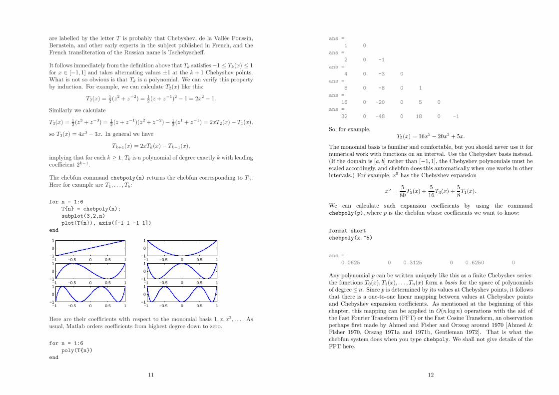
The chebfun command chebpoly(n) returns the chebfun corresponding to Tn.Here for example are T1, . . . , T6:

for n = 1:6

T{n} = chebpoly(n);

subplot(3,2,n)

plot(T{n}), axis([-1 1 -1 1])

end

−1 −0.5 0 0.5 1−1

0

1

−1 −0.5 0 0.5 1−1

0

1

−1 −0.5 0 0.5 1−1

0

1

−1 −0.5 0 0.5 1−1

0

1

−1 −0.5 0 0.5 1−1

0

1

−1 −0.5 0 0.5 1−1

0

1

Here are their coefficients with respect to the monomial basis 1, x, x2, . . . . Asusual, Matlab orders coefficients from highest degree down to zero.

for n = 1:6

poly(T{n})

end

11

ans =

1 0

ans =

2 0 -1

ans =

4 0 -3 0

ans =

8 0 -8 0 1

ans =

16 0 -20 0 5 0

ans =

32 0 -48 0 18 0 -1

So, for example,T5(x) = 16x5 − 20x3 + 5x.

The monomial basis is familiar and comfortable, but you should never use it fornumerical work with functions on an interval. Use the Chebyshev basis instead.(If the domain is [a, b] rather than [−1, 1], the Chebyshev polynomials must bescaled accordingly, and chebfun does this automatically when one works in otherintervals.) For example, x5 has the Chebyshev expansion

x5 =5

80T5(x) +

5

16T3(x) +

5

8T1(x).

We can calculate such expansion coefficients by using the commandchebpoly(p), where p is the chebfun whose coefficients we want to know:

format short

chebpoly(x.^5)

ans =

0.0625 0 0.3125 0 0.6250 0

Any polynomial p can be written uniquely like this as a finite Chebyshev series:the functions T0(x), T1(x), . . . , Tn(x) form a basis for the space of polynomialsof degree ≤n. Since p is determined by its values at Chebyshev points, it followsthat there is a one-to-one linear mapping between values at Chebyshev pointsand Chebyshev expansion coefficients. As mentioned at the beginning of thischapter, this mapping can be applied in O(n log n) operations with the aid ofthe Fast Fourier Transform (FFT) or the Fast Cosine Transform, an observationperhaps first made by Ahmed and Fisher and Orzsag around 1970 [Ahmed &Fisher 1970, Orszag 1971a and 1971b, Gentleman 1972]. That is what thechebfun system does when you type chebpoly. We shall not give details of theFFT here.

12

Just as a polynomial p has a finite Chebyshev series, a more general functionf has an infinite Chebyshev series. Exactly what kind of “more general func-tion” can we allow? For an example like f(x) = ex, everything will turn out tobe straightforward, but what if f is merely differentiable rather than analytic?Or what if it is continuous but not differentiable? Analysts have studied suchcases carefully, identifying exactly what degrees of smoothness correspond towhat kinds of convergence of Chebyshev series. We shall not concern ourselveswith trying to state the sharpest possible result but will just make a particularassumption that covers almost every application. We shall assume that f isLipschitz continuous on [−1, 1]. Recall that this means that there is a con-stant C such that |f(x) − f(y)| ≤ C|x − y| for all x, y ∈ [−1, 1]. Recall alsothat a series is absolutely convergent if it remains convergent if each termis replaced by its absolute value, and that this implies that one can reorder theterms arbitrarily without changing the result.

Here is our basic theorem about Chebyshev series and their coefficients.

Theorem 3.1: Chebyshev series. If f is Lipschitz continuous on [−1, 1], it

has a unique representation as an absolutely and uniformly convergent series

f(x) =

∞∑

k=0

akTk(x),

and the coefficients are given by the formula

ak =2

π

∫ 1

−1

f(x)Tk(x)√1 − x2

dx,

with the special case that for k = 0, the factor 2/π changes to 1/π.

Proof. Throughout this book, our approach to all kinds of results involvingChebyshev polynomials will always be the same: transplant them to the unitcircle in the complex plane, where they become results involving powers of z.Integrals over [−1, 1] transplant to integrals over the unit circle, where one cangenerally get the results one wants from the Cauchy integral formula. Thismethod of dealing with Chebyshev mathematics has the advantage that onenever has to remember any trigonometric identities!

Here is how it goes for Chebyshev series and their coefficients. We are given afunction f(x) on [−1, 1]. We transplant f by defining a function F on the unitcircle whose value at a point z on the circle is the same as the value of f at thecorresponding point x ∈ [−1, 1]. In other words, F (z) = F (z−1) = f(x), wherex = Re z = (z + z−1)/2. Notice that each value x ∈ (−1, 1) corresponds to twodifferent values z on the unit circle, one on the upper semicircle and the otheron the lower semicircle.

To convert between integrals in x and z, we have to convert between dx and dz.

13

We can do this by differentiating the formula for x to get

dx = 12 (1 − z−2) dz = 1

2z−1(z − z−1) dz.

Since12 (z − z−1) = i Im z = ±i

√1 − x2,

this implies

dx = ±i z−1√

1 − x2 dz.

In these equations the plus sign applies for Im z ≥ 0 and the minus sign forIm z ≤ 0.

These formulas have implications for smoothness. Since√

1 − x2 ≤ 1 for allx ∈ [−1, 1], they imply that if f(x) is Lipschitz continuous, then so is F (z).By a standard result in complex variables, this implies that F has a uniquerepresentation as an absolutely and uniformly convergent Laurent series on theunit circle,

F (z) =1

2

∞∑

k=0

ak(zk + z−k) =∞∑

k=0

akTk(x).

Recall that a Laurent series is an infinite series in both positive and negativepowers of z, and that such series in general converge in the interior of an annulus.A good treatment of Laurent series can be found in [Markushevich 1985]. Or onecan derive results about F by converting them to results about Fourier series,for the Laurent series for F is equivalent to a Fourier series in the variable θ ifz = eiθ.

The kth Laurent coefficient of an analytic function G(z) =∑∞

k=−∞ bkzk on theunit circle can be computed by the Cauchy integral formula,

bk =1

2πi

∫

|z|=1

z−1+kG(z) dz.

The notation |z| = 1 indicates that the contour consists of the unit circle tra-versed once in the positive (counterclockwise) direction. Here we have a functionF with the special symmetry property F (z) = F (z−1), and we also have intro-duced a factor 1/2 in front of the series. Accordingly in the case of F we cancompute the coefficients ak from either of two contour integrals,

ak =1

πi

∫

|z|=1

z−1+kF (z) dz =1

πi

∫

|z|=1

z−1−kF (z) dz,

with πi replaced by 2πi for k = 0.

In particular, we can get a formula for ak that is symmetric in k and −k bycombining the two integrals like this:

ak =1

2πi

∫

|z|=1

(z−1+k + z−1−k)F (z) dz =1

πi

∫

|z|=1

z−1 Tk(x)F (z) dz,

14

with πi replaced by 2πi for k = 0. Replacing F (z) by f(x) and z−1dz by−i dx/(±

√1 − x2) gives

ak = − 1

π

∫

|z|=1

f(x)Tk(x)

±√

1 − x2dx,

with π replaced by 2π for k = 0. We have now almost entirely converted tothe x variable, except that the contour of integration is still the circle |z| = 1.When z traverses the unit circle all the way around in the positive direction,x decreases from 1 to −1 and then increases back to 1 again. At the turningpoint z = x = −1, the ± sign attached to the square root switches from + to−. Thus instead of cancelling, the two traverses of x ∈ [−1, 1] contribute equalhalves to ak. Converting to a single integration from −1 to 1 in the x variablemultiplies the integral by −1/2, hence multiplies the formula for ak by −2:

ak =2

π

∫

|z|=1

f(x)Tk(x)√1 − x2

dx.

This is the result stated in the theorem.

The chebfun system represents functions by their values at Chebyshev points.How does it know the right value of n? Given a set of n+1 samples, it convertsthe data to a Chebyshev expansion of degree n and examines the resultingChebyshev coefficients. If these fall below a relative level of approximately10−15, then the grid is judged to be fine enough. For example, here are theChebyshev coefficients of the chebfun corresponding to ex:

f = exp(x);

a = chebpoly(f);

format long

a(end:-1:1)’

ans =

1.266065877752008

1.130318207984970

0.271495339534077

0.044336849848664

0.005474240442094

0.000542926311914

0.000044977322954

0.000003198436463

0.000000199212481

0.000000011036772

0.000000000550590

0.000000000024980

0.000000000001039

15

0.000000000000040

0.000000000000001

Notice that the last coefficient is about at the level of machine precision.

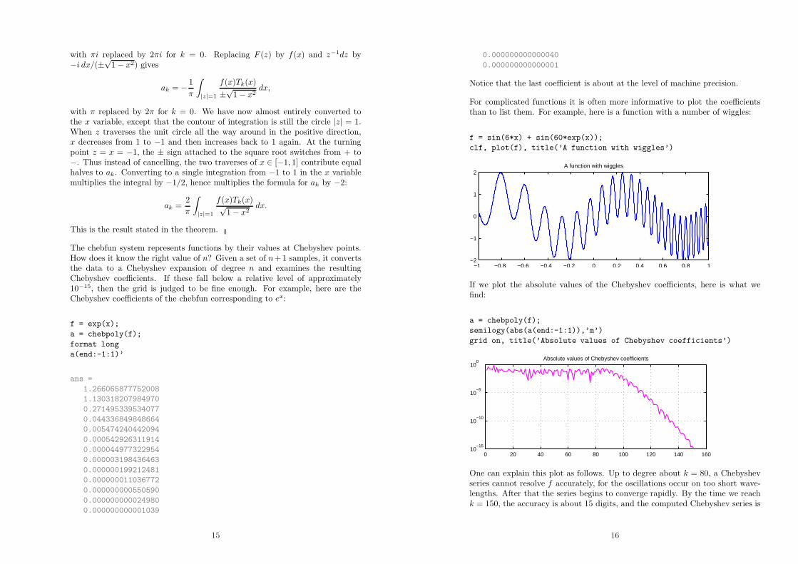
For complicated functions it is often more informative to plot the coefficientsthan to list them. For example, here is a function with a number of wiggles:

f = sin(6*x) + sin(60*exp(x));

clf, plot(f), title(’A function with wiggles’)

−1 −0.8 −0.6 −0.4 −0.2 0 0.2 0.4 0.6 0.8 1−2

−1

0

1

2A function with wiggles

If we plot the absolute values of the Chebyshev coefficients, here is what wefind:

a = chebpoly(f);

semilogy(abs(a(end:-1:1)),’m’)

grid on, title(’Absolute values of Chebyshev coefficients’)

0 20 40 60 80 100 120 140 16010

−15

10−10

10−5

100

Absolute values of Chebyshev coefficients

One can explain this plot as follows. Up to degree about k = 80, a Chebyshevseries cannot resolve f accurately, for the oscillations occur on too short wave-lengths. After that the series begins to converge rapidly. By the time we reachk = 150, the accuracy is about 15 digits, and the computed Chebyshev series is

16

truncated there. We can find out exactly where the truncation took place withthe command length(f):

length(f)

ans =

151

This tells us that the chebfun is a polynomial interpolant through 151 points,that is, of degree 150.

Without giving all the engineering details, here is a fuller description of howthe chebfun system constructs its approximation. First it calculates the poly-nomial interpolant through the function sampled at 9 Chebyshev points, i.e., apolynomial of degree 8, and checks whether the Chebyshev coefficients appearto be small enough. For the example just given the answer is no. Then it tries17 points, then 33, then 65, and so on. In this case the system judges at 257points that the Chebyshev coefficients have finally fallen to the level of round-ing error. At this point it truncates the tail of terms deemed to be negligible,leaving a series of 151 terms. The corresponding degree 150 polynomial is thenevaluated at 151 Chebyshev points via FFT, and these 151 numbers become thedata defining this particular chebfun.

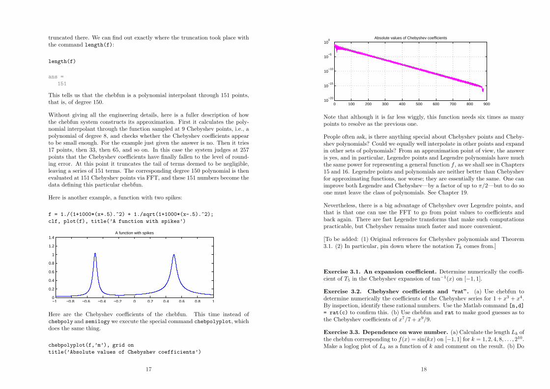
Here is another example, a function with two spikes:

f = 1./(1+1000*(x+.5).^2) + 1./sqrt(1+1000*(x-.5).^2);

clf, plot(f), title(’A function with spikes’)

−1 −0.8 −0.6 −0.4 −0.2 0 0.2 0.4 0.6 0.8 10

0.2

0.4

0.6

0.8

1

1.2

1.4A function with spikes

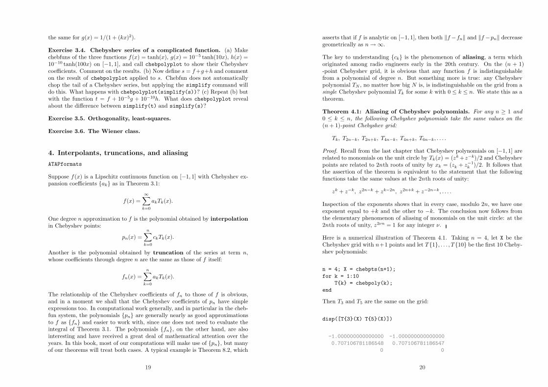
Here are the Chebyshev coefficients of the chebfun. This time instead ofchebpoly and semilogy we execute the special command chebpolyplot, whichdoes the same thing.

chebpolyplot(f,’m’), grid on

title(’Absolute values of Chebyshev coefficients’)

17

0 100 200 300 400 500 600 700 800 90010

−20

10−15

10−10

10−5

100

Absolute values of Chebyshev coefficients

Note that although it is far less wiggly, this function needs six times as manypoints to resolve as the previous one.

People often ask, is there anything special about Chebyshev points and Cheby-shev polynomials? Could we equally well interpolate in other points and expandin other sets of polynomials? From an approximation point of view, the answeris yes, and in particular, Legendre points and Legendre polynomials have muchthe same power for representing a general function f , as we shall see in Chapters15 and 16. Legendre points and polynomials are neither better than Chebyshevfor approximating functions, nor worse; they are essentially the same. One canimprove both Legendre and Chebyshev—by a factor of up to π/2—but to do soone must leave the class of polynomials. See Chapter 19.

Nevertheless, there is a big advantage of Chebyshev over Legendre points, andthat is that one can use the FFT to go from point values to coefficients andback again. There are fast Legendre transforms that make such computationspracticable, but Chebyshev remains much faster and more convenient.

[To be added: (1) Original references for Chebyshev polynomials and Theorem3.1. (2) In particular, pin down where the notation Tk comes from.]

Exercise 3.1. An expansion coefficient. Determine numerically the coeffi-cient of T5 in the Chebyshev expansion of tan−1(x) on [−1, 1].

Exercise 3.2. Chebyshev coefficients and “rat”. (a) Use chebfun todetermine numerically the coefficients of the Chebyshev series for 1 + x3 + x4.By inspection, identify these rational numbers. Use the Matlab command [n,d]

= rat(c) to confirm this. (b) Use chebfun and rat to make good guesses as tothe Chebyshev coefficients of x7/7 + x9/9.

Exercise 3.3. Dependence on wave number. (a) Calculate the length Lk ofthe chebfun corresponding to f(x) = sin(kx) on [−1, 1] for k = 1, 2, 4, 8, . . . , 210.Make a loglog plot of Lk as a function of k and comment on the result. (b) Do

18

the same for g(x) = 1/(1 + (kx)2).

Exercise 3.4. Chebyshev series of a complicated function. (a) Makechebfuns of the three functions f(x) = tanh(x), g(x) = 10−5 tanh(10x), h(x) =10−10 tanh(100x) on [−1, 1], and call chebpolyplot to show their Chebyshevcoefficients. Comment on the results. (b) Now define s = f +g+h and commenton the result of chebpolyplot applied to s. Chebfun does not automaticallychop the tail of a Chebyshev series, but applying the simplify command willdo this. What happens with chebpolyplot(simplify(s))? (c) Repeat (b) butwith the function t = f + 10−5g + 10−10h. What does chebpolyplot revealabout the difference between simplify(t) and simplify(s)?

Exercise 3.5. Orthogonality, least-squares.

Exercise 3.6. The Wiener class.

4. Interpolants, truncations, and aliasing

ATAPformats

Suppose f(x) is a Lipschitz continuous function on [−1, 1] with Chebyshev ex-pansion coefficients {ak} as in Theorem 3.1:

f(x) =

∞∑

k=0

akTk(x).

One degree n approximation to f is the polynomial obtained by interpolation

in Chebyshev points:

pn(x) =

n∑

k=0

ckTk(x).

Another is the polynomial obtained by truncation of the series at term n,whose coefficients through degree n are the same as those of f itself:

fn(x) =

n∑

k=0

akTk(x).

The relationship of the Chebyshev coefficients of fn to those of f is obvious,and in a moment we shall that the Chebyshev coefficients of pn have simpleexpressions too. In computational work generally, and in particular in the cheb-fun system, the polynomials {pn} are generally nearly as good approximationsto f as {fn} and easier to work with, since one does not need to evaluate theintegral of Theorem 3.1. The polynomials {fn}, on the other hand, are alsointeresting and have received a great deal of mathematical attention over theyears. In this book, most of our computations will make use of {pn}, but manyof our theorems will treat both cases. A typical example is Theorem 8.2, which

19

asserts that if f is analytic on [−1, 1], then both ‖f −fn‖ and ‖f −pn‖ decreasegeometrically as n → ∞.

The key to understanding {ck} is the phenomenon of aliasing, a term whichoriginated among radio engineers early in the 20th century. On the (n + 1)-point Chebyshev grid, it is obvious that any function f is indistinguishablefrom a polynomial of degree n. But something more is true: any Chebyshevpolynomial TN , no matter how big N is, is indistinguishable on the grid from asingle Chebyshev polynomial Tk for some k with 0 ≤ k ≤ n. We state this as atheorem.

Theorem 4.1: Aliasing of Chebyshev polynomials. For any n ≥ 1 and

0 ≤ k ≤ n, the following Chebyshev polynomials take the same values on the

(n + 1)-point Chebyshev grid:

Tk, T2n−k, T2n+k, T4n−k, T4n+k, T6n−k, . . . .

Proof. Recall from the last chapter that Chebyshev polynomials on [−1, 1] arerelated to monomials on the unit circle by Tk(x) = (zk +z−k)/2 and Chebyshevpoints are related to 2nth roots of unity by xk = (zk + z−1

k )/2. It follows thatthe assertion of the theorem is equivalent to the statement that the followingfunctions take the same values at the 2nth roots of unity:

zk + z−k, z2n−k + zk−2n, z2n+k + z−2n−k, . . . .

Inspection of the exponents shows that in every case, modulo 2n, we have oneexponent equal to +k and the other to −k. The conclusion now follows fromthe elementary phenomenon of aliasing of monomials on the unit circle: at the2nth roots of unity, z2νn = 1 for any integer ν.

Here is a numerical illustration of Theorem 4.1. Taking n = 4, let X be theChebyshev grid with n+1 points and let T {1}, . . . , T{10} be the first 10 Cheby-shev polynomials:

n = 4; X = chebpts(n+1);

for k = 1:10

T{k} = chebpoly(k);

end

Then T3 and T5 are the same on the grid:

disp([T{3}(X) T{5}(X)])

-1.000000000000000 -1.000000000000000

0.707106781186548 0.707106781186547

0 0

20

-0.707106781186548 -0.707106781186547

1.000000000000000 1.000000000000000

So are T1, T7, and T9:

disp([T{1}(X) T{7}(X) T{9}(X)])

-1.000000000000000 -1.000000000000000 -1.000000000000000

-0.707106781186547 -0.707106781186548 -0.707106781186547

0 0 0

0.707106781186547 0.707106781186548 0.707106781186547

1.000000000000000 1.000000000000000 1.000000000000000

As a corollary of Theorem 4.1, we can now derive the connection between {ak}and {ck}. The following result can be found in [Tadmor 1986], though that isprobably not the earliest reference.

Theorem 4.2: Aliasing formula for Chebyshev coefficients. Let f be

Lipschitz continuous on [−1, 1] and let pn be its Chebyshev interpolant of degree

n with n ≥ 1. Let {ak} and {ck} be the Chebyshev coefficients of f and pn,

respectively. Then

c0 = a0 + a2n + a4n + · · · ,cn = an + a3n + a5n + · · · ,

and for 1 ≤ k ≤ n − 1,

ck = ak + (ak+2n + ak+4n + · · ·) + (a−k+2n + a−k+4n + · · ·).

Proof. By Theorem 3.1, f has a unique Chebyshev series and it convergesabsolutely. Thus we can rearrange the terms of the series without affecting con-vergence, and in particular, each of the three series expansions written aboveconverges, so these formulas do indeed define certain numbers c0, . . . , cn. Tak-ing these numbers as coefficients multiplied by the corresponding Chebyshevpolynomials T0, . . . , Tn gives us a polynomial of degree n. By Theorem 4.1, thispolynomial takes the same values as f at each point of the Chebyshev grid.Thus it is the unique interpolant pn.

We can summarize Theorem 4.2 as follows. On the n+1 point grid, any functionf is indistinguishable from a polynomial of degree n. In particular, the Cheby-shev series of the polynomial interpolant to f is obtained by reassigning all theChebyshev coefficients in the infinite series for f to their aliases of degrees 0through n.

To illustrate Theorem 4.2, here is a function and its degree 4 Chebyshev inter-polant (dashed):

21

f = tanh(4*x-1);

n = 4; pn = chebfun(f,n+1);

hold off, plot(f), hold on, plot(pn,’.--r’)

title(’A function and its degree 4 interpolant’)

−1 −0.8 −0.6 −0.4 −0.2 0 0.2 0.4 0.6 0.8 1−1.5

−1

−0.5

0

0.5

1

1.5A function and its degree 4 interpolant

The first 5 Chebyshev coefficients of f ,

a = chebpoly(f); a = a(end:-1:1)’; a(1:n+1)

ans =

-0.166584582703135

1.193005991160944

0.278438064117869

-0.239362401056012

-0.176961398392888

are different from the Chebyshev coefficients of pn,

c = chebpoly(pn); c = c(end:-1:1)’

c =

-0.203351068209675

1.187719968517890

0.379583465333916

-0.190237989543227

-0.178659622412173

As stated in the theorem, the coefficients c0 and cn are given by sums of coeffi-cients ak with a stride of 2n:

c0 = sum(a(1:2*n:end))

22

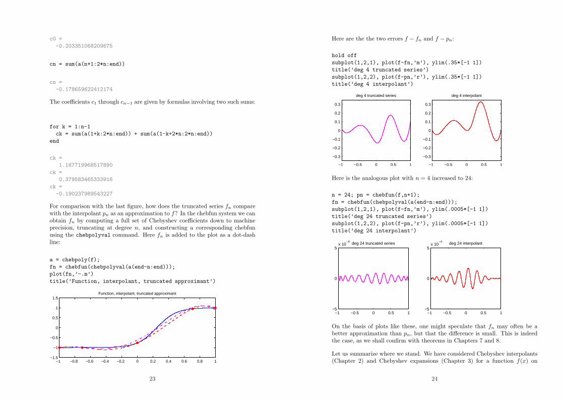
c0 =

-0.203351068209675

cn = sum(a(n+1:2*n:end))

cn =

-0.178659622412174

The coefficients c1 through cn−1 are given by formulas involving two such sums:

for k = 1:n-1

ck = sum(a(1+k:2*n:end)) + sum(a(1-k+2*n:2*n:end))

end

ck =

1.187719968517890

ck =

0.379583465333916

ck =

-0.190237989543227

For comparison with the last figure, how does the truncated series fn comparewith the interpolant pn as an approximation to f? In the chebfun system we canobtain fn by computing a full set of Chebyshev coefficients down to machineprecision, truncating at degree n, and constructing a corresponding chebfunusing the chebpolyval command. Here fn is added to the plot as a dot-dashline:

a = chebpoly(f);

fn = chebfun(chebpolyval(a(end-n:end)));

plot(fn,’-.m’)

title(’Function, interpolant, truncated approximant’)

−1 −0.8 −0.6 −0.4 −0.2 0 0.2 0.4 0.6 0.8 1−1.5

−1

−0.5

0

0.5

1

1.5Function, interpolant, truncated approximant

23

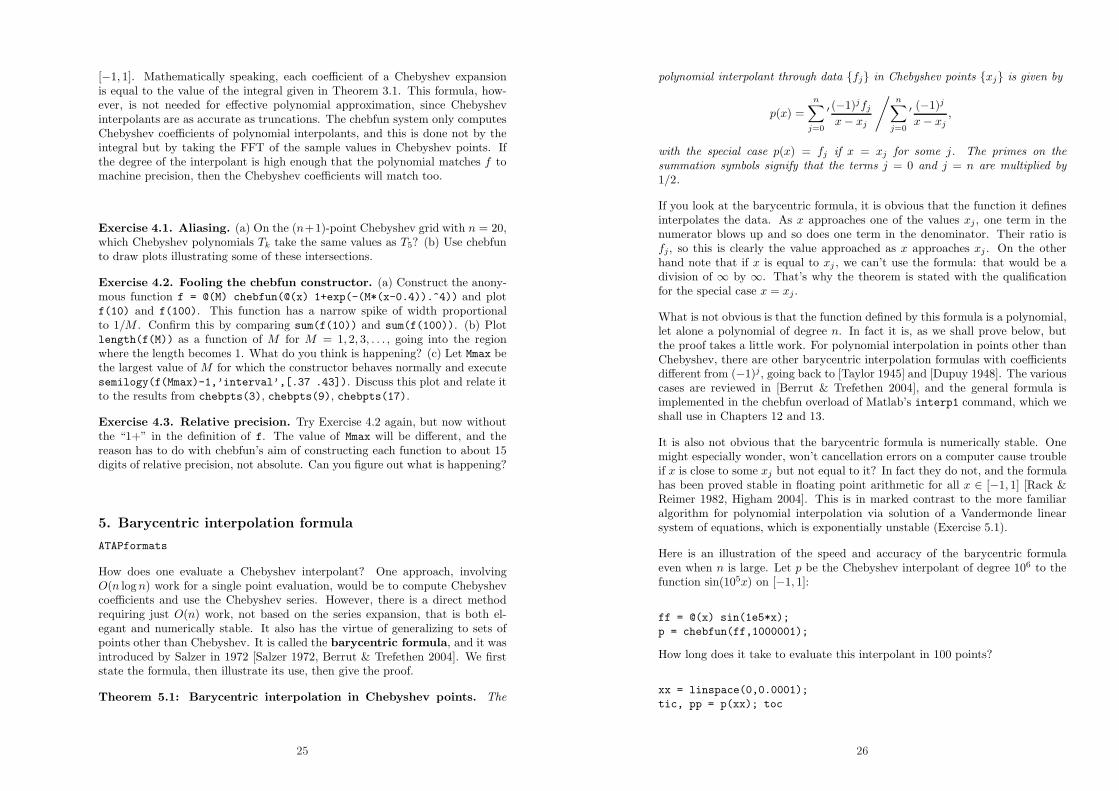
Here are the the two errors f − fn and f − pn:

hold off

subplot(1,2,1), plot(f-fn,’m’), ylim(.35*[-1 1])

title(’deg 4 truncated series’)

subplot(1,2,2), plot(f-pn,’r’), ylim(.35*[-1 1])

title(’deg 4 interpolant’)

−1 −0.5 0 0.5 1

−0.3

−0.2

−0.1

0

0.1

0.2

0.3

deg 4 truncated series

−1 −0.5 0 0.5 1

−0.3

−0.2

−0.1

0

0.1

0.2

0.3

deg 4 interpolant

Here is the analogous plot with n = 4 increased to 24:

n = 24; pn = chebfun(f,n+1);

fn = chebfun(chebpolyval(a(end-n:end)));

subplot(1,2,1), plot(f-fn,’m’), ylim(.0005*[-1 1])

title(’deg 24 truncated series’)

subplot(1,2,2), plot(f-pn,’r’), ylim(.0005*[-1 1])

title(’deg 24 interpolant’)

−1 −0.5 0 0.5 1−5

0

5x 10

−4 deg 24 truncated series

−1 −0.5 0 0.5 1−5

0

5x 10

−4 deg 24 interpolant

On the basis of plots like these, one might speculate that fn may often be abetter approximation than pn, but that the difference is small. This is indeedthe case, as we shall confirm with theorems in Chapters 7 and 8.

Let us summarize where we stand. We have considered Chebyshev interpolants(Chapter 2) and Chebyshev expansions (Chapter 3) for a function f(x) on

24

[−1, 1]. Mathematically speaking, each coefficient of a Chebyshev expansionis equal to the value of the integral given in Theorem 3.1. This formula, how-ever, is not needed for effective polynomial approximation, since Chebyshevinterpolants are as accurate as truncations. The chebfun system only computesChebyshev coefficients of polynomial interpolants, and this is done not by theintegral but by taking the FFT of the sample values in Chebyshev points. Ifthe degree of the interpolant is high enough that the polynomial matches f tomachine precision, then the Chebyshev coefficients will match too.

Exercise 4.1. Aliasing. (a) On the (n+1)-point Chebyshev grid with n = 20,which Chebyshev polynomials Tk take the same values as T5? (b) Use chebfunto draw plots illustrating some of these intersections.

Exercise 4.2. Fooling the chebfun constructor. (a) Construct the anony-mous function f = @(M) chebfun(@(x) 1+exp(-(M*(x-0.4)).^4)) and plotf(10) and f(100). This function has a narrow spike of width proportionalto 1/M . Confirm this by comparing sum(f(10)) and sum(f(100)). (b) Plotlength(f(M)) as a function of M for M = 1, 2, 3, . . . , going into the regionwhere the length becomes 1. What do you think is happening? (c) Let Mmax bethe largest value of M for which the constructor behaves normally and executesemilogy(f(Mmax)-1,’interval’,[.37 .43]). Discuss this plot and relate itto the results from chebpts(3), chebpts(9), chebpts(17).

Exercise 4.3. Relative precision. Try Exercise 4.2 again, but now withoutthe “1+” in the definition of f. The value of Mmax will be different, and thereason has to do with chebfun’s aim of constructing each function to about 15digits of relative precision, not absolute. Can you figure out what is happening?

5. Barycentric interpolation formula

ATAPformats

How does one evaluate a Chebyshev interpolant? One approach, involvingO(n log n) work for a single point evaluation, would be to compute Chebyshevcoefficients and use the Chebyshev series. However, there is a direct methodrequiring just O(n) work, not based on the series expansion, that is both el-egant and numerically stable. It also has the virtue of generalizing to sets ofpoints other than Chebyshev. It is called the barycentric formula, and it wasintroduced by Salzer in 1972 [Salzer 1972, Berrut & Trefethen 2004]. We firststate the formula, then illustrate its use, then give the proof.

Theorem 5.1: Barycentric interpolation in Chebyshev points. The

25

polynomial interpolant through data {fj} in Chebyshev points {xj} is given by

p(x) =

n∑

j=0

′ (−1)jfj

x − xj

/

n∑

j=0

′ (−1)j

x − xj,

with the special case p(x) = fj if x = xj for some j. The primes on the

summation symbols signify that the terms j = 0 and j = n are multiplied by

1/2.

If you look at the barycentric formula, it is obvious that the function it definesinterpolates the data. As x approaches one of the values xj , one term in thenumerator blows up and so does one term in the denominator. Their ratio isfj, so this is clearly the value approached as x approaches xj . On the otherhand note that if x is equal to xj , we can’t use the formula: that would be adivision of ∞ by ∞. That’s why the theorem is stated with the qualificationfor the special case x = xj .

What is not obvious is that the function defined by this formula is a polynomial,let alone a polynomial of degree n. In fact it is, as we shall prove below, butthe proof takes a little work. For polynomial interpolation in points other thanChebyshev, there are other barycentric interpolation formulas with coefficientsdifferent from (−1)j, going back to [Taylor 1945] and [Dupuy 1948]. The variouscases are reviewed in [Berrut & Trefethen 2004], and the general formula isimplemented in the chebfun overload of Matlab’s interp1 command, which weshall use in Chapters 12 and 13.

It is also not obvious that the barycentric formula is numerically stable. Onemight especially wonder, won’t cancellation errors on a computer cause troubleif x is close to some xj but not equal to it? In fact they do not, and the formulahas been proved stable in floating point arithmetic for all x ∈ [−1, 1] [Rack &Reimer 1982, Higham 2004]. This is in marked contrast to the more familiaralgorithm for polynomial interpolation via solution of a Vandermonde linearsystem of equations, which is exponentially unstable (Exercise 5.1).

Here is an illustration of the speed and accuracy of the barycentric formulaeven when n is large. Let p be the Chebyshev interpolant of degree 106 to thefunction sin(105x) on [−1, 1]:

ff = @(x) sin(1e5*x);

p = chebfun(ff,1000001);

How long does it take to evaluate this interpolant in 100 points?

xx = linspace(0,0.0001);

tic, pp = p(xx); toc

26

Elapsed time is 2.203393 seconds.

Not bad for a million-degree polynomial! The result looks fine,

clf, plot(xx,pp,’.’), axis([0 0.0001 -1 1])

title(’A polynomial of degree 10^6 evaluated at 100 points’)

0 0.1 0.2 0.3 0.4 0.5 0.6 0.7 0.8 0.9 1

x 10−4

−1

−0.5

0

0.5

1A polynomial of degree 106 evaluated at 100 points

and it matches the target function closely.

format long

for j = 1:5

r = rand;

disp([ff(r) p(r) ff(r)-p(r)])

end

-0.038787951022018 -0.038787951020191 -0.000000000001827

0.997459577166873 0.997459577165562 0.000000000001311

-0.864212757304804 -0.864212757300479 -0.000000000004326

-0.105230083868529 -0.105230083879794 0.000000000011265

0.911653660186257 0.911653660185483 0.000000000000774

The apparent loss of 4 or 5 digits of accuracy is to be expected since the deriva-tive of this function is of order 105.

Now, using transplantation to the unit circle as in the proofs of Theorems 3.1and 4.1, we derive Salzer’s barycentric formula.

Proof of Theorem 5.1. We start with the observation that the function zn−z−n

has simple roots at the (2n)th roots of unity. Multiplying by z2 − 1 gives afunction zn+2−zn−z2−n +z−n with simple roots at these roots of unity exceptdouble roots at ±1. Now for zj equal to any of the roots of unity, let us divideby (z − zj)(z − zj) to get

rj,n(z) =zn+2 − zn − z2−n + z−n

(z − zj)(z − zj).

27

If zj = ±1, the division cancels the double root and we are left with a functionequal to zero at all the others. If zj is one of the roots of unity other than ±1,the division cancels a conjugate pair of roots and again we have a function thatis zero at all the other roots of unity. In fact, rj,n(z) = 2n(−1)n+j+1 if z is equalto zj or zj and these are 6= ±1, rj,n(z) = 4n(−1)n+j+1 if z = zj = zj = ±1, andrj,n(z) = 0 if z is one of the roots of unity other than zj and zj (Exercise 5.2).

Let us now define the weights

wj = (2n)−1(−1)n+j+1

for zj = ±1 and half this value for zj = ±1. This choice implies that thefunction

wjzn+2 − zn − z2−n + z−n

(z − zj)(z − zj)

equals 1 if z is zj or zj and 0 if it is one of the other roots of unity. By takinga linear combination of these functions for j from 0 to n with coefficients {fj},we get an interpolant through data {fj} satisfying the symmetry conditionfj = f−j ,

n∑

j=0

wjfjzn+2 − zn − z2−n + z−n

(z − zj)(z − zj).

This interpolant takes the value fj at both the points zj and zj, which is justwhat we need for transplantation to Chebyshev points in the unit interval. Infact, since Tk(x) = 1

2 (zk + z−k), this sum is the same as

pn(x) =

n∑

j=0

wjfjTn+2(x) − Tn(x)

x − xj.

This equation is a representation in Lagrange form of the unique polynomial ofdegree ≤n that interpolates the data {fj} in the Chebyshev points {xj}.

A final observation completes the proof. Let the expression just given be dividedby the constant function 1 expressed in the same form. This will not change itsvalue, and the interpolant becomes

pn(x) =

n∑

j=0

wjfjTn+2(x) − Tn(x)

x − xj

/

n∑

j=0

wjTn+2(x) − Tn(x)

x − xj.

Cancelling the common factor Tn+2(x) − Tn(x) gives

28

pn(x) =

n∑

j=0

wjfj

x − xj

/

n∑

j=0

wj

x − xj.

A common factor (2n)−1(−1)n+1 still remains in the weights wj . If this iscancelled, the summation turns into a summation with a prime because thepoints j = 0 and n have half weights, and we are left with the formula statedin the theorem.

Polynomial interpolation is an old subject, going back at least to Newton, whodevised an interpolation formula based on divided differences. The barycentricformula is an example of a Lagrange interpolation formula, in which the inter-polant is written as a linear combination of cardinal functions that are zero atall the interpolation points except one. Lagrange considered such interpolationsin 1795, but the same idea had been treated by Waring in 1779 and Euler in1783 [Waring 1779].

[To be added: (1) Barycentric formula for general points.]

Exercise 5.1. Instability of Vandermonde interpolation. The best-known algorithm for polynomial interpolation, unlike the barycentric formula,is unstable. This is the method implemented in Matlab’s polyfit command,in which one forms a Vandermonde matrix of sampled powers of x and solves acorresponding linear system of equations. (In [Trefethen 2000], for example, thisunstable method is used repeatedly, forcing the values of n employed to be keptnot too large.) (a) Explore this instability by comparing a chebfun evaluationof p(0) with the result of polyval(polyfit(xx,f(xx),n),0) where f = @(x)

cos(k*x) for k = 0, 10, 20, . . . , 100 and n is the degree of the correspondingchebfun. (b) Examining Matlab’s polyfit code as appropriate, construct theVandermonde matrices V for each of these 11 problems and compute their con-dition numbers. By contrast, the underlying Chebyshev interpolation problemis well-conditioned.

Exercise 5.2. Confirmation of values in proof of Theorem 5.1. In theproof of Theorem 5.1, values were stated for the function rj,n at the (2n)th rootsof unity. (a) Show that rj,n(z) = 0 if z is one of the roots of unity other thanzj and zj . (b) Use L’Hopital’s rule and the fact that zn

j = (−1)j to show that

rj,n(z) = 2n(−1)n+j+1 if z is equal to zj or zj and these are 6= ±1. (c) Showthat rj,n(z) = 4n(−1)n+j+1 if z = zj = zj = ±1.

Exercise 5.3. Interpolating the sign function. Use x =

chebfun(’x’), f = sign(x) to construct the sign function on [−1, 1] and p

= chebfun(’sign(x)’,10000) to construct its interpolant in 10000 Chebyshev

29

points. Explore the difference in the interesting region by defining d = f-p, d =

d{-0.002,0.002}. What is the maximum value of d? In what subset of [−1, 1]is it smaller than 0.5 in absolute value?

6. The Weierstrass Approximation Theorem

ATAPformats

Every continuous function on a bounded interval can be approximated to arbi-trary accuracy by polynomials. This is the famous Weierstrass ApproximationTheorem, proved by Karl Weierstrass when he was 70 years old [Weierstrass1885]. The theorem was independently discovered at about the same time,nearly, by Carl Runge: as pointed out by Phragmen and Mittag-Leffler, it canbe derived as a consequence of results Runge published in a pair of papers in1885 and 1886 [Runge 1885 & 1885/1886].

Here and throughout this book, except where indicated otherwise, ‖ · ‖ denotesthe supremum norm on [−1, 1].

Theorem 6.1: Weierstrass Approximation Theorem. Let f be a continu-

ous function on [−1, 1] and let ε > 0 be arbitrary. Then there exists a polynomial

p such that

‖f − p‖ < ε.

Proof. We shall not give a proof in detail. However, here is an outline ofthe beautiful proof from Weierstrass’s original paper. First, extend f(x) toa continuous function f with compact support on the whole real line. Now,take f as initial data at t = 0 for the diffusion equation ∂u/∂t = ∂2u/∂x2

on the real line. It is known that by convolving f with the Gaussian kernelφ(x) = e−x2/4t/

√4πt, we get a solution to this partial differential equation that

converges uniformly to f as t → 0, and thus can be made arbitrarily close to fon [−1, 1] by taking t small enough. On the other hand, since f has compactsupport, for each t > 0 this solution is an integral over a bounded interval ofentire functions and thus itself an entire function, that is, analytic throughoutthe complex plane. Therefore it has a convergent Taylor series on [−1, 1], whichcan be truncated to give polynomial approximations of arbitrary accuracy.

For a fuller presentation of the argument just given as “one of the most amus-ing applications of the Gaussian kernel,” where the result is stated for the moregeneral case of a function of several variables approximated by multivariate poly-nomials, see Chapter 4 of [Folland 1995]. Many other proofs are also known, in-cluding early ones due to Picard (1891), Lerch (1892), Volterra (1897), Lebesgue(1898), Mittag-Leffler (1900), Landau (1908), Jackson (1911), Bernstein (1912),and Montel (1918). This long list gives an idea of the great amount of mathe-matics stimulated by Weierstrass’s theorem and the significant role it played inthe development of analysis in the early 20th century.

30

Weierstrass’s theorem establishes that even extremely non-smooth functionscan be approximated by polynomials, functions like x sin(x−1) or evensin(x−1) sin(1/ sin(x−1)). The latter function has an infinite number of pointsnear which it oscillates infinitely often, as we begin to see from this plot overthe range [0.07, 0.4]. In this calculation the chebfun system is called with auser-prescribed number of interpolation points, 30000, since the usual adaptiveprocedure has no chance of resolving the function to machine precision with apracticable number of points.

f = chebfun(@(x) sin(1./x).*sin(1./sin(1./x)),[.07 .4],3e4);

plot(f), xlim([.07 .4])

title(’A continuous function that is far from smooth’)

0.1 0.15 0.2 0.25 0.3 0.35 0.4−0.4

−0.2

0

0.2

0.4

0.6

0.8

1A continuous function that is far from smooth

We can illustrate the idea of Weierstrass’s proof by showing the convolutionof this complicated function with a Gaussian. Here is the same function frecomputed over a subinterval extending from one of its zeros to another:

r = roots(f{.27,.37});

a = min(r); b = max(r);

f2 = chebfun(@(x) sin(1./x).*sin(1./sin(1./x)),[a,b],2e3);

plot(f), xlim([a b]), title(’Close-up’)

0.29 0.3 0.31 0.32 0.33 0.34 0.35−0.3

−0.2

−0.1

0

0.1

0.2Close−up

31

Here is a narrow Gaussian.

t = 1e-7;

phi = chebfun(@(x) exp(-x.^2/(4*t))/sqrt(4*pi*t),[-.003,.003]);

plot(phi), xlim([-.035 .035])

title(’A narrow Gaussian kernel’)

−0.03 −0.02 −0.01 0 0.01 0.02 0.030

200

400

600

800

1000A narrow Gaussian kernel

Convolving the two gives a smoothed version of f .

f3 = conv(f2,phi);

plot(f3), xlim([a-.003,b+.003])

title(’Convolution of the two’)

0.29 0.3 0.31 0.32 0.33 0.34 0.35−0.3

−0.2

−0.1

0

0.1

0.2Convolution of the two

This is an entire function, readily approximated by polynomials.

For all its beauty, power, and importance, Weierstrass’s theorem has in somerespects served as an unfortunate distraction. Since we know that even trouble-some functions can be approximated by polynomials, it is hard to resist asking,how can we do it? A famous result of Faber in 1914 asserts that there is no setof interpolation points, Chebyshev or otherwise, that achieves convergence asn → ∞ for all f [Faber 1914]. So it becomes tempting to look at approximationmethods that go beyond interpolation, and to warn people that interpolationis not enough, and to try to characterize exactly what minimal properties of f

32

suffice to ensure that interpolation will work after all. A great deal is knownabout these subjects. The trouble with this line of research is, for almost all thefunctions encountered in practice, Chebyshev interpolation works beautifully!Weierstrass’s theorem has encouraged mathematicians over the years to pay toomuch attention to pathological functions at the edge of discontinuity, leading tothe bizarre and unfortunate situation where many books on numerical analysiscaution their readers that interpolation may fail without mentioning that forfunctions with a bit of smoothness, it succeeds outstandingly. For a discussionof the history of such misrepresentations and misconceptions, see Chapter 12.

[To be added: (1) Can we speed up conv?]

Exercise 6.1. A pathological function of Weierstrass. Weierstrass wasone of the first to give an example of a function continuous but nowhere differ-entiable on [−1, 1], and it is one of the early examples of a fractal [Weierstrass1872]:

w(x) =

∞∑

k=0

2−k cos(3kx).

(a) Construct a chebfun w7 corresponding to this series truncated at k = 7. Plotw7, its derivative (use diff), and its indefinite integral (cumsum). What is thedegree of the polynomial defining this chebfun? (b) Prove that w is continuous.(You can use the Weierstrass M-test. In this and the next part, you are free tolook up literature for help.) (c) Prove that w is nondifferentiable at every pointx ∈ [−1, 1].

7. Convergence for differentiable functions

ATAPformats

The principle mentioned at the end of the last chapter might be regarded as thefundamental fact of approximation theory: the smoother a function, the fasterits approximants converge as n → ∞. Connections of this kind were consideredin the early years of the 20th century by three of the founders of approximationtheory: Charles de la Vallee Poussin (1866–1962), a mathematician at Lou-vain in Belgium, Serge Bernstein (1880–1968), a Ukrainian mathematician whohad studied with Hilbert in Gottingen, and Dunham Jackson (1888–1946), anAmerican student of Landau’s also at Gottingen. (Henri Lebesgue in France(1875–1941) also proved some of the early results. For comments on the historysee [Goncharov 2000, Steffens 2006].) Bernstein made the following commentconcerning best approximation errors in his summary article for the Interna-tional Congress of Mathematicians in 1912 [Bernstein 1912a].

Le fait general qui se degage de cette etude est l’existence d’une liaison des plus

33

intimes entre les proprietes differentielles de la fonction f(x) et la loi asympto-

tique de la decroissance des nombres positifs En[f(x)].

[The general fact which emerges from this study is the existence of a very inti-

mate connection between the differential properties of the function f(x) and the

asymptotic rate of decrease of the positive numbers En[f(x)]. ]

In this and the next chapter our aim is to make the smoothness–approximabilitylink precise in the context of Chebyshev truncations and interpolants. Every-thing here is analogous to results for Fourier analysis of periodic functions,and indeed, the whole theory of Chebyshev interpolation can be regarded asa transplant to nonperiodic functions on [−1, 1] of the theory of trigonometricinterpolation of periodic functions on [−π, π].

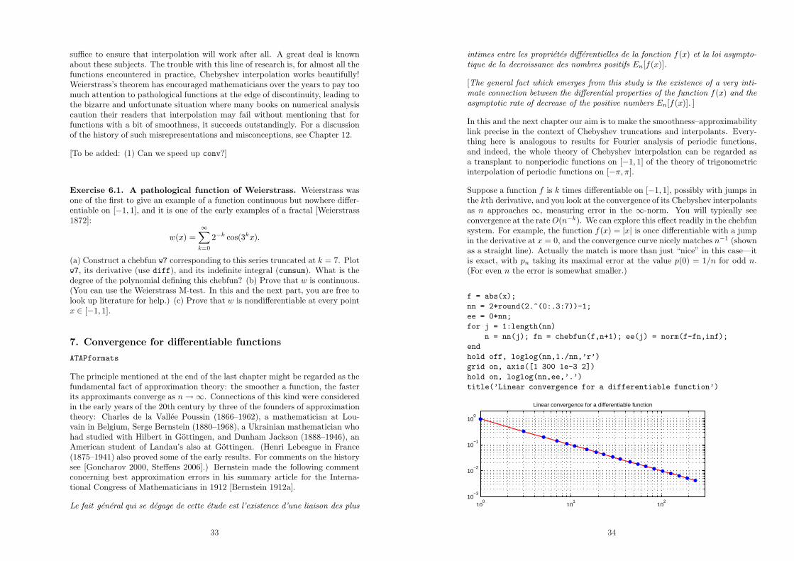
Suppose a function f is k times differentiable on [−1, 1], possibly with jumps inthe kth derivative, and you look at the convergence of its Chebyshev interpolantsas n approaches ∞, measuring error in the ∞-norm. You will typically seeconvergence at the rate O(n−k). We can explore this effect readily in the chebfunsystem. For example, the function f(x) = |x| is once differentiable with a jumpin the derivative at x = 0, and the convergence curve nicely matches n−1 (shownas a straight line). Actually the match is more than just “nice” in this case—itis exact, with pn taking its maximal error at the value p(0) = 1/n for odd n.(For even n the error is somewhat smaller.)

f = abs(x);

nn = 2*round(2.^(0:.3:7))-1;

ee = 0*nn;

for j = 1:length(nn)

n = nn(j); fn = chebfun(f,n+1); ee(j) = norm(f-fn,inf);

end

hold off, loglog(nn,1./nn,’r’)

grid on, axis([1 300 1e-3 2])

hold on, loglog(nn,ee,’.’)

title(’Linear convergence for a differentiable function’)

100

101

102

10−3

10−2

10−1

100

Linear convergence for a differentiable function

34

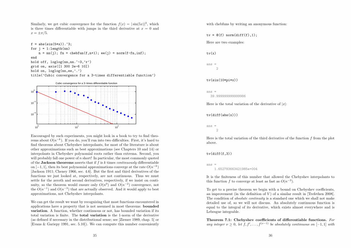
Similarly, we get cubic convergence for the function f(x) = | sin(5x)|3, whichis three times differentiable with jumps in the third derivative at x = 0 andx = ±π/5.

f = abs(sin(5*x)).^3;

for j = 1:length(nn)

n = nn(j); fn = chebfun(f,n+1); ee(j) = norm(f-fn,inf);

end

hold off, loglog(nn,nn.^-3,’r’)

grid on, axis([1 300 2e-6 10])

hold on, loglog(nn,ee,’.’)

title(’Cubic convergence for a 3-times differentiable function’)

100

101

102

10−4

10−2

100

Cubic convergence for a 3−times differentiable function

Encouraged by such experiments, you might look in a book to try to find theo-rems about O(n−k). If you do, you’ll run into two difficulties. First, it’s hard tofind theorems about Chebyshev interpolants, for most of the literature is aboutother approximations such as best approximations (see Chapters 10 and 14) orinterpolants in Chebyshev polynomial roots rather than extrema. Second, youwill probably fall one power of n short! In particular, the most commonly quotedof the Jackson theorems asserts that if f is k times continuously differentiableon [−1, 1], then its best polynomial approximations converge at the rate O(n−k)[Jackson 1911; Cheney 1966, sec. 4.6]. But the first and third derivatives of thefunctions we just looked at, respectively, are not continuous. Thus we mustsettle for the zeroth and second derivatives, respectively, if we insist on conti-nuity, so the theorem would ensure only O(n0) and O(n−2) convergence, notthe O(n−1) and O(n−3) that are actually observed. And it would apply to bestapproximations, not Chebyshev interpolants.

We can get the result we want by recognizing that most functions encountered inapplications have a property that is not assumed in most theorems: bounded

variation. A function, whether continuous or not, has bounded variation if itstotal variation is finite. The total variation is the 1-norm of the derivative(as defined if necessary in the distributional sense; see [Ziemer 1989, chap. 5] or[Evans & Gariepy 1991, sec. 5.10]). We can compute this number conveniently

35

with chebfuns by writing an anonymous function:

tv = @(f) norm(diff(f),1);

Here are two examples:

tv(x)

ans =

2

tv(sin(10*pi*x))

ans =

39.999999999999986

Here is the total variation of the derivative of |x|:

tv(diff(abs(x)))

ans =

2

Here is the total variation of the third derivative of the function f from the plotabove.

tv(diff(f,3))

ans =

1.652783663421985e+004

It is the finiteness of this number that allowed the Chebyshev interpolants tothis function f to converge at least as fast as O(n−3).

To get to a precise theorem we begin with a bound on Chebyshev coefficients,an improvement (in the definition of V ) of a similar result in [Trefethen 2008].The condition of absolute continuity is a standard one which we shall not makedetailed use of, so we will not discuss. An absolutely continuous function isequal to the integral of its derivative, which exists almost everywhere and isLebesgue integrable.

Theorem 7.1: Chebyshev coefficients of differentiable functions. For

any integer ν ≥ 0, let f, f ′, . . . , f (ν−1) be absolutely continuous on [−1, 1] with

36

f (ν) of bounded variation V . Then for k ≥ ν + 1, the Chebyshev coefficients of

f satisfy

|ak| ≤2V

πk(k − 1) · · · (k − ν)≤ 2V

π(k − ν)ν+1.

Proof. As in the proof of Theorem 3.1, setting x = 12 (z + z−1) with z on the

unit circle gives

ak =1

πi

∫

|z|=1

f(12 (z + z−1)) zk−1 dz,

and integrating by parts with respect to z converts this to

ak =−1

πi

∫

|z|=1

f ′(12 (z + z−1))

zk

k

dx

dzdz ;

the factor dx/dz appears since f ′ denotes the derivative with respect to x ratherthan z. Suppose now ν = 0, so that all we are assuming about f is that it isof bounded varation V = ‖f ′‖1. Then we note that this integral over the upperhalf of the unit circle is equivalent to an integral in x ; the integral over the lowerhalf gives another such integral. Combining the two gives

ak =1

πi

∫ 1

−1

f ′(x)zk − zk

kdx =

2

π

∫ 1

−1

f ′(x) Imzk

kdx,

and since |zk/k| ≤ 1/k for x ∈ [−1, 1] and V = ‖f ′‖1, this implies ak ≤ 2V/πk,as claimed.

If ν > 0, we replace dx/dz by 12 (1 − z−2) in the second formula for ak above,

obtaining

ak = − 1

πi

∫

|z|=1

f ′(12 (z + z−1))

[

zk

2k− zk−2

2k

]

dz.

Integrating by parts again with respect to z converts this to

ak =1

πi

∫

|z|=1

f ′′(12 (z + z−1))

[

zk+1

2k(k + 1)− zk−1

2k(k − 1)

]

dx

dzdz.

Suppose now ν = 1 so that we are assuming f ′ has bounded variation V =‖f ′′‖1. Then again this integral is equivalent to an integral in x,

ak =−2

π

∫ 1

−1

f ′′(x) Im

[

zk+1

2k(k + 1)− zk−1

2k(k − 1)

]

dx.

Since the term in square brackets is bounded by 1/k(k − 1) for x ∈ [−1, 1] andV = ‖f ′′‖1, this implies ak ≤ 2V/πk(k − 1), as claimed.

If ν > 1, we continue in this fashion with a total of ν + 1 integrations by partswith respect to z, in each case first replacing dx/dz by 1

2 (1− z−2). At the nextstep the term that appears in square brackets is

[

zk+2

4k(k + 1)(k + 2)− zk

4k2(k + 1)− zk

4k2(k − 1)+

zk−2

4k(k − 1)(k − 2)

]

,

37

which is bounded by 1/k(k − 1)(k − 2) for x ∈ [−1, 1]. And so on.

From Theorems 3.1 and 7.1 we can derive consequences about the accuracy ofChebyshev truncations and interpolants. The second statement of the follow-ing theorem can be found as Corollary 2 in [Mastroianni & Szabados 1995],though with a bound of the form O(n−νV ) rather than an explicit constant,whose appearance here so far as we know is new. The analogous result forbest approximations as opposed to Chebyshev interpolants or truncations wasannounced in [Bernstein 1911] and proved in [Bernstein 1912c].

Theorem 7.2: Convergence for differentiable functions. If f satisfies the

conditions of Theorem 7.1, with V again denoting the total variation of f (ν),

then for any n > ν its Chebyshev truncations satisfy

‖f − fn‖ ≤ 2V

πν(n − ν)ν

and its Chebyshev interpolants satisfy

‖f − pn‖ ≤ 4V

πν(n − ν)ν.

Proof. For the first estimate, Theorem 7.1 gives us

‖f − fn‖ ≤∞∑

k=n+1

|ak| ≤2V

π

∞∑

k=n+1

(k − ν)−ν−1

and this sum can in turn be bounded by

∫ ∞

n

(s − ν)−ν−1ds =1

ν(n − ν)ν.

For the second estimate, we note that by Theorem 4.2, the Chebyshev inter-polants satisfy the same bound except with coefficients 2|ak| rather than |ak|.

Here is a way to remember the O(n−ν) message of Theorem 7.2. Suppose wetry to approximate the step function sign(x) by polynomials. There is no hopeof convergence, since polynomials are continuous and sign(x) is not, so all wecan achieve is accuracy O(1) as n → ∞. That’s the case ν = 0. But now, eachtime we make the function “one derivative smoother,” ν increases by 1 and sodoes the order of convergence.

How sharp is Theorem 7.2 for our example functions? In the case of f(x) = |x|,with ν = 1 and V = 2, it predicts ‖f − fn‖ ≤ 4/π(n − 1) and ‖f − pn‖ ≤8/π(n−1) ≈ 2.55/(n−1). As mentioned above, the actual value for Chebyshevinterpolation is ‖f − pn‖ = 1/n for odd n. The minimal possible error in poly-nomial approximation, with pn replaced by the best approximation p∗n (Chapter

38

10), is ‖f − p∗n‖ ∼ 0.280169 . . .n−1 as n → ∞ [Varga & Carpenter 1985]. So wesee that the range from best approximant, to Chebyshev interpolant, to boundon Chebyshev interpolant is less than a factor of 10. The approximation of |x|was a central problem studied by de la Vallee Poussin, Bernstein, and Jacksonin the 1910s.

The results are similar for the other example, f(x) = | sin(5x)|3, whose thirdderivative, we saw, has variation V ≈ 16528. Theorem 7.2 implies that theChebyshev interpolants satisfy ‖f − pn‖ < 7020/(n − 1)3, whereas in fact, wehave ‖f − pn‖ ≈ 309/n3 for large odd n and ‖f − p∗n‖ ≈ 80/n3.

We close with a comment about Theorem 7.2. We have assumed in this theoremthat f (ν) is of bounded variation. A similar but weaker condition would bethat f (ν−1) is Lipschitz continuous (Exercise 7.2). This weaker assumption isenough to ensure ‖f − p∗n‖ = O(n−ν) for the best approximations {p∗n}; thisis one of the Jackson theorems. On the other hand it is not enough to ensureO(n−ν) convergence of Chebyshev truncations and interpolants. The reason weemphasize the stronger condition with the stronger conclusion is that in practiceone rarely deals with a function that is Lipschitz continuous while lacking aderivative of bounded variation, whereas one constantly deals with truncationsand interpolants rather than best approximations.

Incidentally it was de la Vallee Poussin in 1908 who first showed that the stronghypothesis is enough to reach the weak conclusion: if f (ν) is of bounded vari-ation, then ‖f − p∗n‖ = O(n−ν) for the best approximation p∗n [de la ValleePoussin 1908]. Three years later Jackson sharpened the result by weakening thehypothesis [Jackson 1911].

[To be added: (1) Converse of Thm 7.2. (2) Jackson and other literature?]

Exercise 7.1. Total variation. Determine numerically the total variation off(x) = sin(100x)/(1 + x2) on [−1, 1].

Exercise 7.2. Lipschitz continuous vs. derivative of bounded variation.

(a) Show that if the derivative f ′ of a function f has bounded variation, then fis Lipschitz continuous. (b) Show that the converse does not hold.

Exercise 7.3. Convergence for Weierstrass’s function. Exercise 6.1 con-sidered a “pathological function of Weierstrass” w(x) which is continuous butnowhere differentiable on [−1, 1]. Use chebfun to produce plots of ‖f − fn‖ and‖f − pn‖ accurate enough and for high enough values of n to confirm visuallythat convergence appears to take place as n → ∞. Thus w is not one of thefunctions for which interpolants fail to converge, a fact we shall prove in Chapter13 while also showing how such troublesome functions can be constructed.

39

8. Convergence for analytic functions

ATAPformats

Suppose f is not just k times differentiable but infinitely differentiable and infact analytic on [−1, 1]. (Recall that this means that for any s ∈ [−1, 1], f has aTaylor series about s that converges to f in a neighborhood of s.) Then withoutany further assumptions we may conclude that the Chebyshev truncations andinterpolants converge geometrically, that is, at the rate O(C−n) for someconstant C > 1. This means the errors will look like straight lines (or better)on a semilog scale rather than a loglog scale. This kind of connection was firstannounced by Bernstein in 1911, who showed that the best approximations toa function f on [−1, 1] converge geometrically as n → ∞ if and only if f isanalytic [Bernstein 1911 & 1912c].

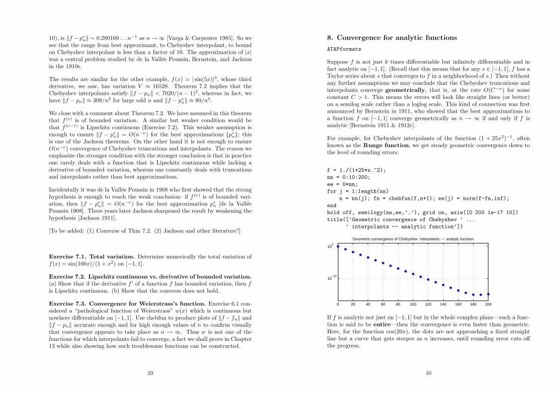
For example, for Chebyshev interpolants of the function (1 + 25x2)−1, oftenknown as the Runge function, we get steady geometric convergence down tothe level of rounding errors:

f = 1./(1+25*x.^2);

nn = 0:10:200;

ee = 0*nn;

for j = 1:length(nn)

n = nn(j); fn = chebfun(f,n+1); ee(j) = norm(f-fn,inf);

end

hold off, semilogy(nn,ee,’.’), grid on, axis([0 200 1e-17 10])

title([’Geometric convergence of Chebyshev ’ ...

’ interpolants -- analytic function’])

0 20 40 60 80 100 120 140 160 180 200

10−10

100

Geometric convergence of Chebyshev interpolants −− analytic function

If f is analytic not just on [−1, 1] but in the whole complex plane—such a func-tion is said to be entire—then the convergence is even faster than geometric.Here, for the function cos(20x), the dots are not approaching a fixed straightline but a curve that gets steeper as n increases, until rounding error cuts offthe progress.

40

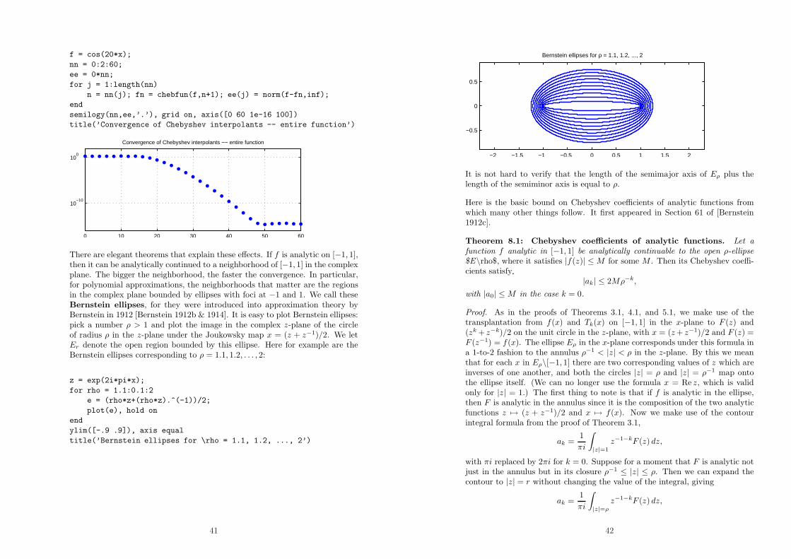
f = cos(20*x);

nn = 0:2:60;

ee = 0*nn;

for j = 1:length(nn)

n = nn(j); fn = chebfun(f,n+1); ee(j) = norm(f-fn,inf);

end

semilogy(nn,ee,’.’), grid on, axis([0 60 1e-16 100])

title(’Convergence of Chebyshev interpolants -- entire function’)

0 10 20 30 40 50 60

10−10

100

Convergence of Chebyshev interpolants −− entire function

There are elegant theorems that explain these effects. If f is analytic on [−1, 1],then it can be analytically continued to a neighborhood of [−1, 1] in the complexplane. The bigger the neighborhood, the faster the convergence. In particular,for polynomial approximations, the neighborhoods that matter are the regionsin the complex plane bounded by ellipses with foci at −1 and 1. We call theseBernstein ellipses, for they were introduced into approximation theory byBernstein in 1912 [Bernstein 1912b & 1914]. It is easy to plot Bernstein ellipses:pick a number ρ > 1 and plot the image in the complex z-plane of the circleof radius ρ in the z-plane under the Joukowsky map x = (z + z−1)/2. We letEr denote the open region bounded by this ellipse. Here for example are theBernstein ellipses corresponding to ρ = 1.1, 1.2, . . . , 2:

z = exp(2i*pi*x);

for rho = 1.1:0.1:2

e = (rho*z+(rho*z).^(-1))/2;

plot(e), hold on

end

ylim([-.9 .9]), axis equal

title(’Bernstein ellipses for \rho = 1.1, 1.2, ..., 2’)

41

−2 −1.5 −1 −0.5 0 0.5 1 1.5 2

−0.5

0

0.5

Bernstein ellipses for ρ = 1.1, 1.2, ..., 2

It is not hard to verify that the length of the semimajor axis of Eρ plus thelength of the semiminor axis is equal to ρ.

Here is the basic bound on Chebyshev coefficients of analytic functions fromwhich many other things follow. It first appeared in Section 61 of [Bernstein1912c].

Theorem 8.1: Chebyshev coefficients of analytic functions. Let a

function f analytic in [−1, 1] be analytically continuable to the open ρ-ellipse$E\rho$, where it satisfies |f(z)| ≤ M for some M . Then its Chebyshev coeffi-cients satisfy

|ak| ≤ 2Mρ−k,

with |a0| ≤ M in the case k = 0.

Proof. As in the proofs of Theorems 3.1, 4.1, and 5.1, we make use of thetransplantation from f(x) and Tk(x) on [−1, 1] in the x-plane to F (z) and(zk + z−k)/2 on the unit circle in the z-plane, with x = (z + z−1)/2 and F (z) =F (z−1) = f(x). The ellipse Eρ in the x-plane corresponds under this formula ina 1-to-2 fashion to the annulus ρ−1 < |z| < ρ in the z-plane. By this we meanthat for each x in Eρ\[−1, 1] there are two corresponding values of z which areinverses of one another, and both the circles |z| = ρ and |z| = ρ−1 map ontothe ellipse itself. (We can no longer use the formula x = Re z, which is validonly for |z| = 1.) The first thing to note is that if f is analytic in the ellipse,then F is analytic in the annulus since it is the composition of the two analyticfunctions z 7→ (z + z−1)/2 and x 7→ f(x). Now we make use of the contourintegral formula from the proof of Theorem 3.1,

ak =1

πi

∫

|z|=1

z−1−kF (z) dz,

with πi replaced by 2πi for k = 0. Suppose for a moment that F is analytic notjust in the annulus but in its closure ρ−1 ≤ |z| ≤ ρ. Then we can expand thecontour to |z| = r without changing the value of the integral, giving

ak =1

πi

∫

|z|=ρ

z−1−kF (z) dz,

42

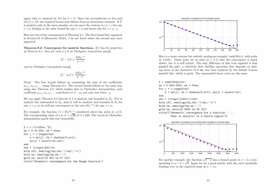
again with πi replaced by 2πi for k = 0. Since the circumference is 2πρ and|F (z)| ≤ M , the required bound now follows from an elementary estimate. If Fis analytic only in the open annulus, we can move the contour to |z| = s for anys < ρ, leading to the same bound for any s < ρ and hence also for s = ρ.

Here are two of the consequences of Theorem 8.1. The first bound first appearedin Section 61 of [Bernstein 1912c]. I do not know where the second may haveappeared.

Theorem 8.2: Convergence for analytic functions. If f has the properties

of Theorem 8.1, then for each n ≥ 0 its Chebyshev truncations satisfy

‖f − fn‖ ≤ 2Mρ−n

ρ − 1

and its Chebyshev interpolants satisfy

‖f − pn‖ ≤ 4Mρ−n

ρ − 1.

Proof. The first bound follows by estimating the sum of the coefficientsan+1, an+2, . . . using Theorem 8.1. The second bound follows in the same wayusing also Theorem 4.2, which implies that in Chebyshev interpolation, eachcoefficient an+1, an+2, . . . contributes to f − pn not once but twice.

We can apply Theorem 8.2 directly if f is analytic and bounded in Eρ. If it isanalytic but unbounded in Eρ, then it will be analytic and bounded in Es forany s < ρ, so we still get convergence at the rate O(s−n) for any s < ρ.

For example, the function (1 + 25x2)−1 considered above has poles at ±i/5.The corresponding value of ρ is (1 +

√26)/5 ≈ 1.220. The errors in Chebyshev

interpolation match this rate beautifully:

f = 1./(1+25*x.^2);

nn = 0:10:200; ee = 0*nn;

for j = 1:length(nn)

n = nn(j); fn = chebfun(f,n+1);

ee(j) = norm(f-fn,inf);

end

rho = (1+sqrt(26))/5;

hold off, semilogy(nn,rho.^(-nn),’-r’)

hold on, semilogy(nn,ee,’.’)

grid on, axis([0 200 1e-17 10])

title(’Geometric convergence for the Runge function’)

43

0 20 40 60 80 100 120 140 160 180 200

10−10

100

Geometric convergence for the Runge function

Here is a more extreme but entirely analogous example: tanh(50πx), with polesat ±0.01i. These poles are so close to [−1, 1] that the convergence is muchslower, but it is still robust. The only difference in this code segment is thatnorm(f-fn,inf), a relatively slow chebfun operation that depends on find-ing zeros of the derivative of f-fn, has been replaced by the default 2-normnorm(f-fn), which is quick. The exponential decay rates are the same.

f = tanh(50*pi*x);

nn = 0:200:4000; ee = 0*nn;

for j = 1:length(nn)

n = nn(j); fn = chebfun(f,n+1); ee(j) = norm(f-fn);

end

rho = (1+sqrt(10001))/100;

hold off, semilogy(nn,rho.^(-nn),’-r’)

hold on, semilogy(nn,ee,’.’)

grid on, axis([0 4000 1e-16 10])

title([’Geometric convergence for a function ’ ...

’that is analytic in a narrow region’])

0 500 1000 1500 2000 2500 3000 3500 4000

10−10

100

Geometric convergence for a function that is analytic in a narrow region

For another example, the function√

2 − x has a branch point at x = 2, corre-sponding to ρ = 2 +

√3. Again we see a good match, with the curve gradually

bending over to the expected slope as n → ∞.

44

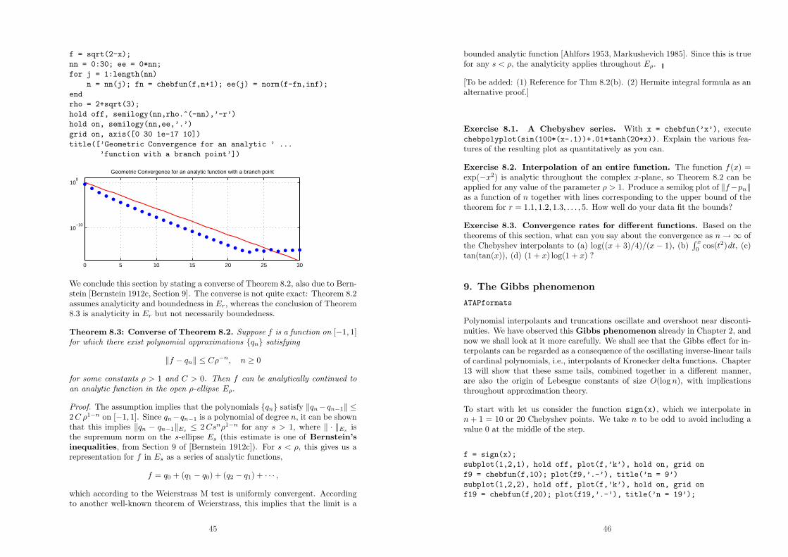
f = sqrt(2-x);

nn = 0:30; ee = 0*nn;

for j = 1:length(nn)

n = nn(j); fn = chebfun(f,n+1); ee(j) = norm(f-fn,inf);

end

rho = 2+sqrt(3);

hold off, semilogy(nn,rho.^(-nn),’-r’)

hold on, semilogy(nn,ee,’.’)

grid on, axis([0 30 1e-17 10])

title([’Geometric Convergence for an analytic ’ ...

’function with a branch point’])

0 5 10 15 20 25 30

10−10

100

Geometric Convergence for an analytic function with a branch point

We conclude this section by stating a converse of Theorem 8.2, also due to Bern-stein [Bernstein 1912c, Section 9]. The converse is not quite exact: Theorem 8.2assumes analyticity and boundedness in Er, whereas the conclusion of Theorem8.3 is analyticity in Er but not necessarily boundedness.

Theorem 8.3: Converse of Theorem 8.2. Suppose f is a function on [−1, 1]for which there exist polynomial approximations {qn} satisfying

‖f − qn‖ ≤ Cρ−n, n ≥ 0

for some constants ρ > 1 and C > 0. Then f can be analytically continued to

an analytic function in the open ρ-ellipse Eρ.

Proof. The assumption implies that the polynomials {qn} satisfy ‖qn− qn−1‖ ≤2 C ρ1−n on [−1, 1]. Since qn−qn−1 is a polynomial of degree n, it can be shownthat this implies ‖qn − qn−1‖Es

≤ 2 Csnρ1−n for any s > 1, where ‖ · ‖Esis

the supremum norm on the s-ellipse Es (this estimate is one of Bernstein’s

inequalities, from Section 9 of [Bernstein 1912c]). For s < ρ, this gives us arepresentation for f in Es as a series of analytic functions,

f = q0 + (q1 − q0) + (q2 − q1) + · · · ,

which according to the Weierstrass M test is uniformly convergent. Accordingto another well-known theorem of Weierstrass, this implies that the limit is a

45

bounded analytic function [Ahlfors 1953, Markushevich 1985]. Since this is truefor any s < ρ, the analyticity applies throughout Eρ.

[To be added: (1) Reference for Thm 8.2(b). (2) Hermite integral formula as analternative proof.]

Exercise 8.1. A Chebyshev series. With x = chebfun(’x’), executechebpolyplot(sin(100*(x-.1))+.01*tanh(20*x)). Explain the various fea-tures of the resulting plot as quantitatively as you can.

Exercise 8.2. Interpolation of an entire function. The function f(x) =exp(−x2) is analytic throughout the complex x-plane, so Theorem 8.2 can beapplied for any value of the parameter ρ > 1. Produce a semilog plot of ‖f−pn‖as a function of n together with lines corresponding to the upper bound of thetheorem for r = 1.1, 1.2, 1.3, . . . , 5. How well do your data fit the bounds?

Exercise 8.3. Convergence rates for different functions. Based on thetheorems of this section, what can you say about the convergence as n → ∞ ofthe Chebyshev interpolants to (a) log((x + 3)/4)/(x − 1), (b)

∫ x

0 cos(t2)dt, (c)tan(tan(x)), (d) (1 + x) log(1 + x) ?

9. The Gibbs phenomenon

ATAPformats

Polynomial interpolants and truncations oscillate and overshoot near disconti-nuities. We have observed this Gibbs phenomenon already in Chapter 2, andnow we shall look at it more carefully. We shall see that the Gibbs effect for in-terpolants can be regarded as a consequence of the oscillating inverse-linear tailsof cardinal polynomials, i.e., interpolants of Kronecker delta functions. Chapter13 will show that these same tails, combined together in a different manner,are also the origin of Lebesgue constants of size O(log n), with implicationsthroughout approximation theory.

To start with let us consider the function sign(x), which we interpolate inn + 1 = 10 or 20 Chebyshev points. We take n to be odd to avoid including avalue 0 at the middle of the step.

f = sign(x);

subplot(1,2,1), hold off, plot(f,’k’), hold on, grid on

f9 = chebfun(f,10); plot(f9,’.-’), title(’n = 9’)

subplot(1,2,2), hold off, plot(f,’k’), hold on, grid on

f19 = chebfun(f,20); plot(f19,’.-’), title(’n = 19’);

46