Approximation of the

Quadratic Knapsack Problem∗

Ulrich Pferschy ∗∗ Joachim Schauer ∗∗

Abstract

We study the approximability of the classical quadratic knapsack prob-lem (QKP) on special graph classes. In this case the quadratic terms ofthe objective function are not given for each pair of knapsack items. In-stead an edge weighted graph G = (V, E) whose vertices represent theknapsack items induces a quadratic profit pij for the items i and j when-ever they are adjacent in G (i.e (i, j) ∈ E). We show that the problempermits an FPTAS on graphs of bounded treewidth and a PTAS on planargraphs and more generally on H-minor free graphs. This result is shownby adopting a technique of Demaine et al. (2005). We also show strongNP-hardness of QKP on graphs that are 3-book embeddable, a naturalgraph class that is related to planar graphs. In addition we will argue thatthe problem is likely to have a bad approximability behaviour on all graphclasses that include the complete graph or contain large cliques. Thesehardness of approximation results under certain complexity assumptionscarry over from the densest k-subgraph problem.

Keywords: quadratic knapsack problem, special graph classes,

approximation algorithm, book embedding, densest k-subgraph.

1 Introduction

In the standard 0-1 knapsack problem (KP) we are given a set of n items eachwith an integer profit pj and weight wj . We look for a subset of items whose totalweight does not exceed a given capacity c and whose total profit is maximized.

If some pairs of items i, j are interdependent and generate a certain synergy,we gain an additional nonnegative profit pij if both i and j are included inthe solution set. This defines the Quadratic Knapsack Problem (QKP), seee.g. Kellerer et al. (2004, Sec.12) or Pisinger (2007).

∗A preliminary, short version of this paper appeared in Pferschy and Schauer (2013).∗∗University of Graz, Department of Statistics and Operations Research, Universi-

taetsstr. 15, A-8010 Graz, Austria, pferschy, joachim.schauer@uni-graz.at

1

To represent which items are in relation to each other, we introduce a graphG = (V, E) with |V | = n and |E| = m. Every vertex v ∈ V corresponds uniquelyto an item and an edge (u, v) ∈ E indicates that the two corresponding itemsyield an additional profit, if they are both included in the solution. We will usevertex and item interchangeable. Using binary variables xj with xj = 1 iff itemj is included in the solution, QKP can be defined as follows:

(QKP ) max

n∑

i=1

pixi +∑

(i,j)∈E

pijxixj (1)

s.t.

n∑

i=1

wixi ≤ c (2)

xi ∈ 0, 1, i = 1, . . . , n (3)

W.l.o.g. we can assume that wj ≤ c for all j and for every edge (i, j) ∈ E thereis wi + wj ≤ c. Otherwise, items i and j could never be packed together andwe can remove the edge (i, j) since its profit pij could never contribute to anyfeasible solution.

QKP is a challenging strongly NP-hard problem. Indeed, the notoriously hardmaximum clique problem can be reduced to it: Given a graph G, we set wj = 1and pj = 0 for all j and assign profits pij = 1 for all (i, j) ∈ E. Solving QKPwith c = k, it follows that G contains a clique of size k iff the optimal solution

of QKP is k(k−1)2 . Going through all values of k (or performing binary search)

identifies the maximum clique.

There is a wide range of literature presenting exact solution algorithms for QKP,in particular procedures to derive upper bounds to be used in branch and boundschemes. The currently best performing exact algorithm was given by Pisingeret al. (2007).

On the other hand, very little is know about the approximation of QKP. It isan open question whether a constant approximation ratio for QKP is possible.Note that for the modified problem, where also negative profit values are allowed,Rader Jr. and Woeginger (2002) showed that no constant approximation ratiocan be achieved in polynomial time (under P6=NP).

A natural approach to fill this void is the consideration of special cases of QKP,in particular restrictions to graphs with special properties. So far, the onlyresult in this direction is an FPTAS for QKP on series parallel graphs based ondynamic programming given by Rader Jr. and Woeginger (2002). On the otherhand, they show that QKP on so-called vertex series parallel graphs is stronglyNP-hard and thus does not permit an FPTAS (under P6=NP).

A very special variant of QKP was considered from an approximation pointof view by Kellerer and Strusevich (2010, 2012). They introduced a so-calledsymmetric quadratic knapsack problem where also pairs of not-included items

2

contribute a quadratic profit and the coefficients pij have a special multiplicativestructure. A recent improvement of their work is due to Xu (2012).

1.1 Connections to the densest k-subgraph problem

It is common in the literature that optimization problems with bad approxima-tion behavior on general graphs are studied on certain restricted graph classessince in many cases it turned out that the approximability on these restrictedgraph classes can be much better than on a general graph. Very prominentgraph classes in this context are trees, graphs of bounded treewidth, planargraphs, chordal graphs and comparability graphs (amongst others). For QKPhowever this strategy might already fail on proper interval graphs and thus onchordal graphs as well as on many other basic graph classes due to the followingconnection to the densest k-subgraph problem.

The densest k-subgraph problem on a general graph G = (V, E) asks for aninduced subgraph G′ = (V ′, E′) of G, where |V ′| = k and |E′| is maximized.

From a hardness of approximation point of view DkS is a notorious problem.The best known hardness result under P 6= NP is the strong NP-hardnessderived from the maximum clique problem (cf. Feige et al. (2001)). Howeverunder stronger complexity assumptions several inapproximability results wereshown in the last years, mostly by using and developing very involved tech-niques: Feige (2002) ruled out the existence of a PTAS based on an assumptiondealing with average-case hardness of random 3-SAT. Khot (2006) ruled out theexistence of a PTAS under the assumption that NP does not have randomizedsubexponential time algorithms. Alon et al. (2011) showed that under a hard-ness assumption on random k-AND formulas, there will not exist any constantfactor approximation for DkS. They also pointed out that Raghavendra et al.(2010) showed the same result under the Small Set Expansion Conjecture. Alonet al. (2011) even proved superconstant hardness of approximation results forDkS under an hardness assumptions dealing with the Hidden Clique problem.

From an approximation point of view any QKP instance on an n vertex graphG can be modelled by the complete graph Kn

1. Make G complete by addingall missing edges and assign a profit of 0 to them. Therefore any DkS instanceI can be transformed into a QKP instance J on Kn in the following way: foreach vertex in I introduce a vertex with weight 1 and profit 0 in J . For eachedge in I add the same edge to J with profit 1. Introduce all missing edgeswith profit 0 in J in order to get a Kn and set the capacity c = k. Clearly thissimple transformation is approximation preserving.

Therefore we can immediately state the following result.

1Kn denotes the complete graph with n vertices.

3

Theorem 1. QKP is at least as hard to approximate on any graph class con-taining graphs with n vertices and cliques of size nε (for some constant ε) asthe densest k-subgraph problem on general graphs.

In particular, Theorem 1 applies to any graph class containing the completegraph. Hence, finding a good approximation algorithm for QKP on one of thefollowing very prominent and basic graph classes would break one of the citedhardness assumption (depending on the quality of the approximation): properinterval graphs and all superclasses such as chordal graphs; graphs of boundedclique-width; comparability and co-comparability graphs; distance hereditarygraphs; AT-free graphs.

Since rank-width is bounded iff clique-width is bounded (cf. Oum and Seymour(2006)), and a complete graph has clique-width 2, the hardness results hold alsofor graphs of bounded rank-width.

While the above reduction indicates that QKP and DkS have strong similaritiesin their approximability behavior, this analogy breaks down completely for densegraphs. It was shown by Arora et al. (1999) that there exists a PTAS for DkSon graphs with Ω(n2) edges for k in Ω(n) (and DkS becomes trivial on completegraphs), while an instance of QKP can always be extended to a complete graphby adding edges with profit 0 without gaining anything w.r.t. approximability.

Another breach of analogy occurs e.g. for interval graphs, where DkS permitsa PTAS as recently shown by Nonner (2011) while Theorem 1 applies for QKP.

Outlook: It is an interesting open question to find hardness of approximationresults for QKP under the standard assumption P 6= NP . In particular, canone find such a result by using properties of QKP that go beyond DkS? Webelieve that the global capacity constraint of QKP is not very helpful in showingsuch a result and thus we conjecture that finding negative approximation resultsfor QKP is as hard as for DkS.

1.2 Contributions of this paper

We will make considerable progress in answering the question of approximabilityfor QKP. Our contribution is threefold:

1. An FPTAS for QKP on graphs of bounded treewidth (which includes theclass of series parallel graphs) is given in Section 2.

2. For graphs that do not include any fixed graph H as a minor, a PTAS isderived in Section 3. This includes planar graphs.

These two contributions are the first meaningful approximation results for QKPon special graph classes since Rader Jr. and Woeginger (2002).

4

3. In Section 4 we show that QKP on 3-book embeddable graphs is stronglyNP-hard.

The result on 3-book embeddable graphs is important since this is the first hard-ness result for QKP which has no connection to the maximum clique problemor closely related variants.

k-book embeddable graphs generalize the concept of planarity in a natural way.Planar graphs are very interesting for DkS, since the complexity status of DkSremains open on them (cf. Chen et al. (2011)) 2. Note that the standard reduc-tion for showing NP-hardness of DkS, i.e. the reduction from the maximumclique problem, does not work on planar graphs. In any case, our results ofSection 3 also imply a PTAS for the densest k-subgraph problem on planargraphs.

Overbay (2007) proved that the embedding of a complete graph on n verticesneeds a book with ⌈n

2 ⌉ pages. Therefore, a k-book embeddable graph withconstant k can have a maximum clique of size at most 2k and can be found byenumeration. But this means that the reduction of DkS from maximum cliquedoes not work on k-book embeddable graphs with constant k.

Note that the existence of an FPTAS for QKP on planar graphs and, moregeneral, on any H-minor-free graph remains open. However such an FPTASwould optimally solve DkS on planar graphs and thus resolve this long standingopen problem.

2 QKP on Graphs of Bounded Treewidth

In this section we present an FPTAS for graphs of bounded treewidth. Clearly,this includes graphs of bounded pathwidth. The result also extends to graphs ofbounded cutwidth and bounded bandwidth, since these parameters are at leastas large as the pathwidth (see Bodlaender (1998, Sec. 9)). The same appliesfor graphs of bounded branchwidth, which is within a constant factor of thetreewidth.

We assume that P is an upper bound on the optimal solution value, e.g. P :=∑n

i=1 pi +∑

(i,j)∈E pij , if no better bound is available. We will show that givena tree-decomposition of constant treewidth k, QKP can be solved by dynamicprogramming in O(nP 2) time. By applying standard rounding arguments thisalgorithms can be used to derive an FPTAS. Note that the framework anddefinitions of this section are closely related to Pferschy and Schauer (2009,Sec. 2), where the knapsack problem with conflict graphs was considered forconflict graphs of bounded treewidth.

2Keil and Brecht (1991) proved that DkS is NP-hard when the selected k vertex subgraphhas to be connected.

5

2.1 Tree Decompositions

Diestel (2006) defines a tree-decomposition of a graph G = (V, E) in the follow-ing way: Let T be a tree with vertex set V (T ) where every vertex I ∈ V (T )corresponds to a subset of V . Formally, let V = (VI)I∈V (T ) be a family of ver-tex sets VI ⊆ V (G) indexed by the vertices I of T . By capital letters we referto vertices from T , whereas by lower case letters we refer to vertices from G.The pair (T,V) is called a tree-decomposition if it satisfies the following threeproperties:

1. V (G) =⋃

I∈T VI .

2. for every edge (u, v) ∈ E(G) there exists I ∈ T such that both u ∈ VI andv ∈ VI .

3. If I2 lies on the path from I1 to I3 in T , then VI1 ∩ VI3 ⊆ VI2 .

The width of (T,V) is defined as max|VI | − 1 | I ∈ T . The treewidth of G isthe smallest width of any tree-decomposition of G (Diestel (2006)). Recall thattrees have treewidth 1, while e.g. series parallel graphs have treewidth 2.

By Bodlaender (1996) deciding whether a tree-decomposition of treewidth atmost k exists, and if so, finding such a tree-decomposition can be done in lineartime if k is seen as a constant and not as part of the input.

For algorithmic purposes a specially structured tree-decomposition, namely anice tree-decomposition turned out to be useful in many applications. This tree-decomposition has the property of being a binary tree in which adjacent verticescorrespond to vertex sets of G that differ by at most one vertex. One vertex Ris considered to be the root of T and each vertex I ∈ T is of one of the followingfour types (Bodlaender and Koster (2008)):

• Leaf : vertex I is a leaf of T and |VI | = 1.

• Join : vertex I has exactly two children J1 and J2, and VI = VJ1= VJ2

.

• Introduce : vertex I has exactly one child J , and there is a vertex v ∈ Vwith VI = VJ ∪ v.

• Forget : vertex I has exactly one child J , and there is a vertex v ∈ V withVJ = VI ∪ v.

Furthermore, given an arbitrary tree-decomposition of width k, Bodlaender andKoster (2008) described how to find a nice tree-decomposition of width at mostk with O(n) tree vertices in linear time. For some vertex I of T we denote by(T (I),V) the tree-decomposition limited to the subtree T (I) of T rooted in I.Clearly (T (I),V) is no longer a tree-decomposition of G. Let furthermore GI bethe subgraph of G that is induced by (T (I),V), more precisely by

⋃

J∈T (I) VJ .

6

2.2 Dynamic Programming Algorithm

Let (T,V) be a nice tree-decomposition of G of bounded treewidth k. For somevertex J in T , let UJ be the set of subsets S of vertices from VJ with the propertythat

∑

i∈S wi ≤ c (UJ includes the empty set ∅). Now we define the followingfunction for a dynamic programming approach:

Let fSd (J) be the minimum weight of an item set including the set

S ⊆ VJ with total profit equal to d, while considering only the limitedtree-decomposition (T (J),V).

Related to the approach pursued in Bodlaender and Koster (2008) and Pferschyand Schauer (2009) we solve QKP by algorithm AlgQBT described as Algo-rithm 1. AlgQBT processes the given tree-decomposition in depth-first order.The optimal solution is finally represented by an entry of the dynamic program-ming array for the root vertex R of the tree-decomposition with maximum profitd and feasible weight, i.e. fS

d (R) ≤ c.

Theorem 2. Algorithm AlgQBT solves QKP on a graph G of bounded treewidthk to optimality.

Proof.

Given a nice tree-decomposition we will show by an induction like procedure thatfor each vertex I ∈ T AlgQBT computes an optimal solution for the subgraphGI of G. First the optimality is proved for leaf vertices of T . Then for eachinner vertex J ∈ T the optimality of GJ will be proved, given that for the atmost two children I1 and I2 of J the induced subgraphs GI1 and GI2 are solvedoptimally. Since G = GR the result follows.

Leaf vertices. By the depth-first search structure of the recursion, someleaf vertex I of T is the first vertex processed by AlgQBT. By definition of anice tree-decomposition, VI consists of exactly one vertex v ∈ G, so GI equalsa subgraph containing only v. By (a) in Algorithm 1 when including v intothe knapsack solution (constrained to GI) the only possible profit d = pv hasweight wv.

Inner vertices.

Introduce with respect to vertex v. Let I be an Introduce (line (b) in AlgQBT)with child vertex J . By assumption AlgQBT computed the solutions for GJ

optimally. Since GI \v = GJ , all solutions in GI not containing v were alreadycomputed in GJ and hence remain optimal also for GI . If a solution contains vthe algorithm correctly computes the minimum weight for each profit value d:all neighbors of v in GI are included in I, otherwise we would get a contradictionto property 2 and 3 of a tree-decomposition. Finally, the optimality follows sincethe profit contributed by vertex v and a set S ⊆ VI is given by

pv +∑

u∈S

puv

7

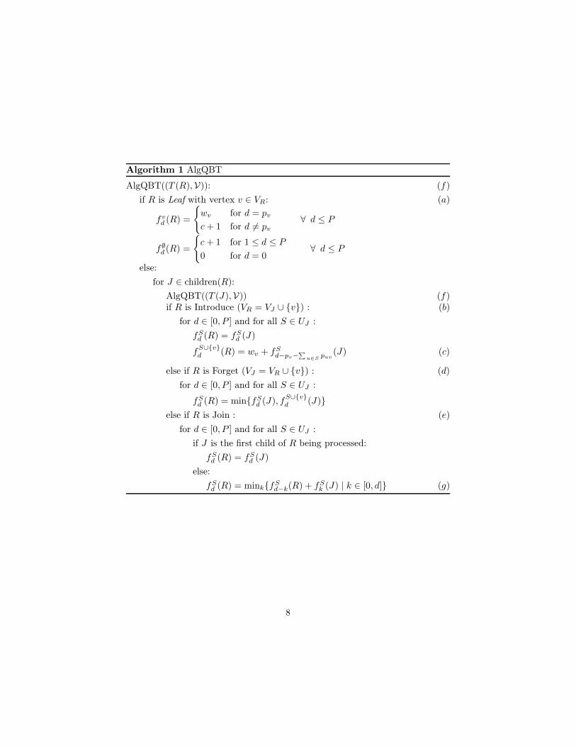
Algorithm 1 AlgQBT

AlgQBT((T (R),V)): (f)

if R is Leaf with vertex v ∈ VR: (a)

fvd (R) =

wv for d = pv

c + 1 for d 6= pv

∀ d ≤ P

f∅d (R) =

c + 1 for 1 ≤ d ≤ P

0 for d = 0∀ d ≤ P

else:

for J ∈ children(R):

AlgQBT((T (J),V)) (f)if R is Introduce (VR = VJ ∪ v) : (b)

for d ∈ [0, P ] and for all S ∈ UJ :

fSd (R) = fS

d (J)

fS∪vd (R) = wv + fS

d−pv−∑

u∈Spuv

(J) (c)

else if R is Forget (VJ = VR ∪ v) : (d)

for d ∈ [0, P ] and for all S ∈ UJ :

fSd (R) = minfS

d (J), fS∪vd (J)

else if R is Join : (e)

for d ∈ [0, P ] and for all S ∈ UJ :

if J is the first child of R being processed:

fSd (R) = fS

d (J)

else:

fSd (R) = minkfS

d−k(R) + fSk (J) | k ∈ [0, d] (g)

8

and the algorithm computes in (c) for each profit d and S the combination ofthe weight of v with the previously computed minimal weight in G(J) requiredto reach profit d.

Forget with respect to vertex v. Let I be a Forget with child vertex J (line (d)in AlgQBT): then GI = GJ and the optimality of fS

d (I) for each subset S ⊆ VI

and profit d follows from the minimum expression by induction.

Join. Let I be a Join with children J1 and J2 (line (e) in AlgQBT). For thefirst child the correctness is obvious. For the second child, AlgQBT calculatesfor each set S ∈ VI the minimum weight of a knapsack solution leading to aprofit of d by computing in (g) the minimum over all possible combinations ofweights from the subgraphs GJ1

and GJ2. By assumption both of these parts

are optimal and by property 2 and 3 of a tree-decomposition the intersectionof the neighborhood N(GJ1

\ G(VI)) with GJ2\ G(VI) is the empty set (G(VI )

denotes the subgraph of G induced by VI), i.e. all connections between GJ1and

GJ2are induced by vertices of VI . Hence, we did not loose any quadratic profit

terms by combining solutions of the different parts of the Join.

Theorem 3. Algorithm AlgQBT has a running time of O(2knP 2) and requiresO(2knP ) space given a nice tree-decomposition (T,V) with O(n) vertices andtreewidth k.

Proof.

Time Complexity. Since the nice tree-decomposition has O(n) vertices, AlgQBTconsists of O(n) recursive calls (f) in Algorithm 1. Since for each vertex set VI ,I ∈ T , at most 2k+1 subsets of vertices of G have to be considered, AlgQBTcomputes solutions for O(2k) subsets S ⊆ VI and O(P ) profit values in eachline where the dynamic programming array is updated. All these updates canbe performed in constant time with the exception of part (g). There we take foreach profit value the minimum over d+1 combinations of weights for each profitvalue. Thus, each evaluation of part (g) requires O(P ) time and the overall timecomplexity follows.

Space Complexity. For each vertex I ∈ T , each feasible subset S ⊆ VI and eachprofit d the minimum weight is stored yielding a space complexity of O(2knP ).

2.3 FPTAS for QKP on Graphs of Bounded Treewidth

A fully polynomial approximation scheme for QKP on graphs of bounded treewidthcan be derived by applying the standard rounding argument for the knapsackproblem (cf. Kellerer et al. (2004, Sec. 2.6) or Rader Jr. and Woeginger (2002))to the dynamic programming algorithm AlgQBT. The profits pj and pij arereplaced by scaled profits pj := ⌊pj

K⌋ and pij := ⌊pij

K⌋, for some K to be defined

later. Then the problem is solved to optimality by AlgQBT with the scaledprofit values yielding an optimal solution set X. Generally, this set will be

9

different from the solution set X∗ which optimizes the original instance with asolution value of z∗. The set X is taken as an approximate solution with solu-tion value zA obtained for the original profits. Clearly zA ≤ z∗. Then one getsthe following chain of inequalities, where E(X) ⊆ E denotes the edges inducedby a vertex set X ⊆ V .

zA =∑

j∈X

pj +∑

(i,j)∈E(X)

pij ≥∑

j∈X

K⌊pj

K⌋ +

∑

(i,j)∈E(X)

K⌊pij

K⌋

≥∑

j∈X∗

K(pj

K− 1) +

∑

(i,j)∈E(X∗)

K(pij

K− 1)

=∑

j∈X∗

(pj − K) +∑

(i,j)∈E(X∗)

(pij − K) = z∗ − (|X∗| + |E(X∗)|)K

To bound the relative error of the approximation algorithm by a given value εwe get the following inequality:

z∗ − zA

z∗≤

(|X∗| + |E(X∗)|)K

z∗≤

(n + m)K

z∗≤ ε

Define the largest coefficient of the objective function as pmax := max maxpj |j = 1, . . . , n, maxpij | (i, j) ∈ E. Clearly, z∗ ≥ pmax, since each single itemand each pair of items (i, j) ∈ E is a feasible solution. Choosing K := ε pmax

n+m

trivially satisfies the required condition.

Furthermore, in the running time and space complexity of AlgQBT the trivialupper bound P can be replaced for the scaled instance in the following way: theoptimal solution value z of the scaled problem instance is bounded by

z ≤ (n + m) pmax ≤ (n + m)pmax

K=

(n + m)2

ε. (4)

Therefore, in the running time bound for the FPTAS derived from algorithm

AlgQBT one can replace the factor P by (n+m)2

εfor the scaled instances.

The number of edges m can be bounded by the following well-known fact (seee.g. Rose (1974)).

Proposition 4. For a graph G = (V, E) of treewidth at most k, the number ofedges can be bounded by

|E| ≤ k |V | −1

2k(k + 1).

Thus, the upper bound on P given in (4) is in O( (kn)2

ε) and the complexity of

the FPTAS can be stated as follows.

Theorem 5. There is an FPTAS for QKP on graphs of treewidth k requiring

running time O(2kk4 n5

ε2 ) and O(2kk2 n3

ε) space.

10

3 PTAS for QKP on Certain Graph Classes

An important graph class for which QKP was not considered yet is the classof planar graphs. It is well known that this class can be defined by forbiddingthe K3,3 and the K5 as a minor.3 In this section we will show that planargraphs admit a PTAS for QKP. More generally, by applying a structural resultof Demaine et al. (2005) we will show that a PTAS exists for QKP on all graphclasses defined by a fixed excluded minor H . By Lovász (2006) a graph His a minor of G if H can be obtained by successively applying the followingthree operations on G: deleting isolated vertices, deleting edges and contractingedges. Moreover a class of graphs C is called H-minor free if the graph H is nota minor of any of the graphs of C.

Demaine et al. (2005) showed the following decomposition theorem:

Theorem 6. Demaine et al. (2005, Theorem 3.1) For a fixed graph H, thereis a constant cH such that, for any integer k ≥ 2 and for every H-minor-freegraph G, the vertices of G can be partitioned into k sets such that any k − 1 ofthe sets induce a graph of treewidth at most cHk. Furthermore, such a partitioncan be found in polynomial time.

We can use this decomposition to obtain a PTAS for QKP under the samescenario.

Theorem 7. There is a PTAS for QKP on H-minor-free graphs for any fixedgraph H.

Proof.

We first compute in polynomial time a decomposition of V into k (which willbe determined later) disjoint subsets V1, . . . , Vk as given by Theorem 6. Eachvertex set Vj induces an edge set Ej . For each subset ℓ ∈ 1, . . . , k we defineby Eℓ the set of edges between Vℓ and V \Vℓ, i.e. the edges joining Vℓ with othersubsets Vj , j 6= ℓ. Removing all edges in Eℓ from the graph we obtain a graphG′

ℓ consisting of the graph induced by the k−1 remaining sets of vertices of thepartition and a disconnected part induced by Vℓ. According to Theorem 6 bothof these two parts have bounded treewidth and so has their union G′

ℓ.

For the optimal variable values x∗i the optimal solution value of QKP on G can

be written as

z∗ =∑

i∈V

pix∗i +

k∑

ℓ=1

∑

(i,j)∈Eℓ

pijx∗i x

∗j +

1

2

k∑

ℓ=1

∑

(i,j)∈Eℓ

pijx∗i x

∗j , (5)

where the second term sums up all edges within one subset Vℓ while the thirdterm sums over all edges between Vℓ and all other subsets. Since G is an undi-rected graph, every edge appears twice in the latter expression which necessitatesthe factor 1

2 .

3Ka,b denotes a complete bipartite graph with vertex sets containing a resp. b vertices.

11

Choosing

ℓ∗ := argk

minℓ=1

∑

(i,j)∈Eℓ

pijx∗i x

∗j

(6)

we obtain the set Vℓ∗ with the smallest profit contribution of edges between Vℓ∗

and all other subsets. By the usual averaging argument we have

∑

(i,j)∈Eℓ∗

pijx∗i x

∗j ≤

1

k

k∑

ℓ=1

∑

(i,j)∈Eℓ

pijx∗i x

∗j . (7)

Removing all edges in Eℓ∗ we obtain a graph G′ℓ∗ of bounded treewidth (see

above). The optimal solution of QKP on this reduced graph G′ℓ∗ yields an

optimal solution value zℓ∗ which can be bounded by (7)

zℓ∗ ≥ z∗ −∑

(i,j)∈Eℓ∗

pijx∗i x

∗j ≥ z∗ −

1

k

k∑

ℓ=1

∑

(i,j)∈Eℓ

pijx∗i x

∗j .

(x∗i still denotes the optimal solution on the full graph.) Bounding generously

with only the third term of (5) we get

zℓ∗ ≥ z∗ −1

k· 2 z∗ =

(

1 −2

k

)

z∗.

Since we cannot find the optimal solution of QKP on G′ℓ∗ in polynomial time, we

have to make use of the FPTAS from Theorem 5 to compute a δ-approximationzA of zℓ∗ . This yields

zA ≥ (1 − δ)zℓ∗ ≥ (1 − δ)(1 −2

k) z∗.

For δ := ε2 and k := ⌈ 2ε⌉ + 2 we get zA ≥ (1 − ε)z∗ as required for a PTAS.

Of course, we can not find ℓ∗ without knowing the optimal solution. Instead,we ge through all k possible choices of ℓ∗ and run the PTAS on each candidategraph G′

ℓ for ℓ = 1, . . . , k. Taking the best of these k approximate solutionvalues guarantees a solution value at least as large as zA.

Planar graphs are a subclass of K3,3-minor free (resp. K5-minor free) graphs.Thus, Theorem 6 and therefore our algorithm apply to planar graphs as well.However the above PTAS for the case of a planar graph G could be simplifiedby a construction closely related to Baker’s approach described in Baker (1994).In fact, taking a planar embedding of the graph, certain layers of vertices can beremoved in order to get a k-outerplanar subgraph of the original graph, whichis known to have treewidth at most 3k − 1 (cf. Bodlaender (1996)).

Going through all k possible choices of removing layers, we have to solve ktimes an FPTAS on such a graph of treewidth 3k − 1. Plugging in the result ofTheorem 5 for treewidth 3⌈ 2

ε⌉ + 5 and accuracy ε2 yields the following result.

12

Corollary 8. There is a PTAS for QKP on planar graphs with running timeO(2

6

ε n5/ε9).

Applying the simple, approximation preserving reduction from Section 1.1 wecan also state the following consequence of Theorem 7:

Corollary 9. There is a PTAS for DkS on H-minor-free graphs for any fixedgraph H (and thus on planar graphs).

4 Hardness for 3-book embeddings

In this section, we show that QKP is strongly NP-hard on graphs that are3-book embeddable. This result is interesting since a k-book embedding gen-eralizes the concept of planar graphs (however not characterized by forbiddenminors). Furthermore the NP-hardness proofs for densest k subgraph and QKPon special graph classes presented in the literature are based on the maximumclique problem or on closely related variants (cf. Rader Jr. and Woeginger(2002), Corneil and Perl (1984)), whereas our reduction follows a completelydifferent approach.

A k-book consists of k half planes, called pages, whose common intersectionis a line, called the spine. A k-book embedding of a graph G = (V, E) is anembedding of G into a k-book such that all vertices are arranged on the spineand each edge e = (u, v) is embedded into a unique page where the intersectionof e with the spine consists only of u and v (cf. Chung et al. (1987)). Clearlyevery graph has a |E|-book embedding. For planar graphs it was shown byYannakakis (1989) that a book of four pages is sufficient for an embedding. Itis an open question whether four pages are also necessary, as conjectured inYannakakis (1989).

It is easy to see that graphs with a 1-book embedding are exactly the outerplanargraphs (join the two ends of the spine). Since outerplanar graphs have treewidthat most 2, it follows from Theorem 5 that there is an FPTAS for QKP on 1-bookembeddable graphs.

2-book embeddable graphs are known to be a subclass of planar graphs (seefurther below). Thus, Theorem 7 (or Corollary 8) implies a PTAS for QKP on2-book embeddable graphs, while the existence of an FPTAS remains an openquestion.

The main result of this section rules out an FPTAS for QKP on 3-book em-beddable graphs. However, the existence of a PTAS remains open. The samesituation applies for arbitrary k-book embeddable graphs with k ≥ 4 and QKPin general.

In our hardness proof we will reduce a special variant of 3SAT to QKP on 3-book embeddable graphs: Moore and Robson (2001) showed that Cubic Planar

13

bc bc bc r bc r r bc bc bcbc bc

x1

x2 xj

c1

ci

Page 1

Page 2

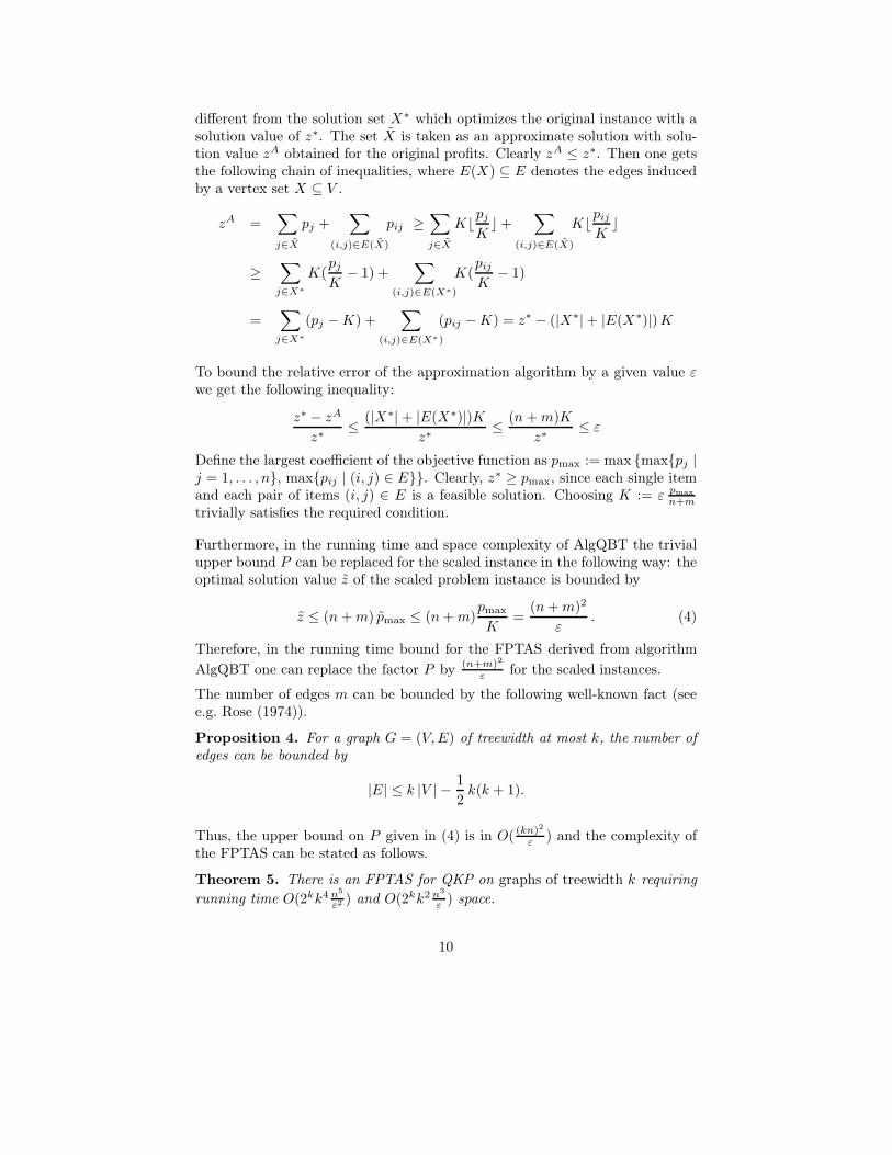
Figure 1: A 2-book embedding of GSAT

Monotone 1-in-3 SAT (CPM-1-3-SAT ) is strongly NP-hard. In this problemn clauses and n variables are given, where each clause contains exactly threevariables and each variable occurs in exactly three clauses. Monotone meansthat this problem does not contain negated literals. Moreover the graph GSAT

that represents each variable and clause by a unique vertex and introduces edgesbetween them whenever a variable appears in a clause is planar. A feasiblesolution to CPM-1-3-SAT consists of exactly n

3 variables set TRUE such thateach clause contains exactly one variable set TRUE.

Let I be an instance of CPM-1-3-SAT and GSAT its corresponding graph.Kainen and Overbay (2003) showed that any planar graph with girth (shortestcycle) > 3 is a subgraph of a planar Hamiltonian graph. Moreover it is wellknown that a graph is 2-book embeddable if and only if it is the subgraph of aplanar Hamiltonian graph (cf. Bernhart and Kainen (1979)). Therefore GSAT ,which is bipartite and thus has no cycle of length 3, has a 2-book embedding.

In the following proof we will transform this 2-book embedding of the CPM-1-3-SAT instance I into a QKP instance J defined on a graph GJ that is 3-bookembeddable. Note that the transformation will not preserve planarity.

The construction of GJ

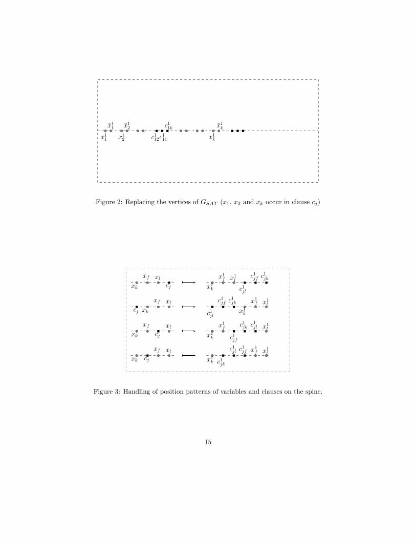
Let GSAT be represented by a 2-book embedding as in Figure 1 (here the dotsrepresent vertices and the squares clauses). We first represent the vertices xi

of GSAT by vertices x1i and x1

i in GJ and the cj vertices of GSAT by threevertices c1

jk, where the index k denotes that variable xk occurs in clause cj (seeFigure 2). We call them vertices of layer 1 and denote the layer by a superscript

14

bc bc bc r bc rbc bcbc bc bc r r bc bc bc r r

x11

x11

x12

x12

c111c1

12

c11k

x1k

x1k

Figure 2: Replacing the vertices of GSAT (x1, x2 and xk occur in clause cj)

bc bc bc r

xk

xf

cj

xlbc bc bc r

x1k

x1f

c1jl

x1l r r

c1jf c1

jk

bc bc bcr

xk

xf

cj

xlbc bc bcr

x1k

x1f

c1jl

x1lr r

c1jf c1

jk

bc bc bcr

xk

xf

cj

xlbc bc bcr

x1k

x1f

c1jf

x1lr r

c1jk c1

jl

bc bc bcr

xk

xf

cj

xlbc bc bcr

x1k

x1f

c1jk

x1lr r

c1jl c1

jf

Figure 3: Handling of position patterns of variables and clauses on the spine.

15

c11k

x21x2

1c211 c2

12c21kc1

12c111x1

2x11 x1

2x11

bc bc bc rbc bc bc r r bcbcrbc bc bcbcr rbc bcx2

2 x22

bc bc

Figure 4: Duplicating vertices from layer 1 to layer 2.

x72x7

1 x72x7

1

bc bc bc rbc bc bc r r bc bc bcbcbcbc

Figure 5: Case i = 2: Adjencies of x72 on layer i + 5 = 7

index. Figure 3 describes how the vertices c1ik are arranged with respect to the

four possible position patterns of the variables xk, xf and xl and the clause cj

on the spine of GSAT .

Next we duplicate (in fact mirror) these vertices n + 4 times. This is done byintroducing vertices xℓ

i , xℓi and cℓ

jk, ℓ = 2, . . . , n+5, on n+4 new layers. The ver-

tices xℓi get associated a profit and weight of n24, the vertices xℓ

i get associateda profit and weight of n18 and the vertices cℓ

jk get associated a profit and weight

of n12. Furthermore the following edges are introduced: (xℓi , x

ℓ+1i ), (xℓ

i , xℓ+1i ),

and (cℓjk, cℓ+1

jk ) (cf. Figure 4, rectangular edges). An edge (xℓi , x

ℓ+1i ) gets asso-

ciated a profit of n21, an edge (xℓi , x

ℓ+1i ) gets associated a profit of n15 and an

edge (cℓjk, cℓ+1

jk ) gets associated a profit of n9. Note that after this duplicationprocedure on layers 1 and n + 5 two book pages remain unused, whereas on allother layers only one book page remains unused. On one remaining book pageof layer 1 we connect all vertices x1

i with the corresponding vertex c1ji, whenever

variable xi occurs in clause cj (see Figure 4, curvy edges) and a weight of n3 isassigned to these edges. On layer 5 + i we connect x5+i

i to all x5+ij with j 6= i

and associate a profit of n6 to these edges (cf. Figure 5 for layer 7).

16

bc bc bcr

xl

bc bc bc r

xk xf cj

bc bc bc r

x2k x2

f c2jlx2

l

r r

c2jf c2

jk

bc bc bcr

xk xfcj xl

bc bc bcr

x2k x2

fc2jl x2

l

r r

c2jf c2

jk

bc bc bcr

xk xf cj xl

bc bc bcr

x2k x2

f c2jf x2

l

r r

c2jk c2

jl

xk xfcj xl

bc bc bcr

x2k x2

fc2jk x2

l

r r

c2jl c2

jf

Page 1 of GSAT

bc bc bc r

x3k x3

f c3jlx3

lr r

c3jf c3

jk

Remaining page of layer 2 Remaining page of layer 3

bc bc bcr

x3k x3

fc3jl x3

lr r

c3jf c3

jk

bc bc bcr

x3k x3

f c3jf x3

lr r

c3jk c3

jl

bc bc bcr

x3k x3

fc3jk x3

lr r

c3jl c3

jf

Figure 6: Representing adjacent vertices of GSAT

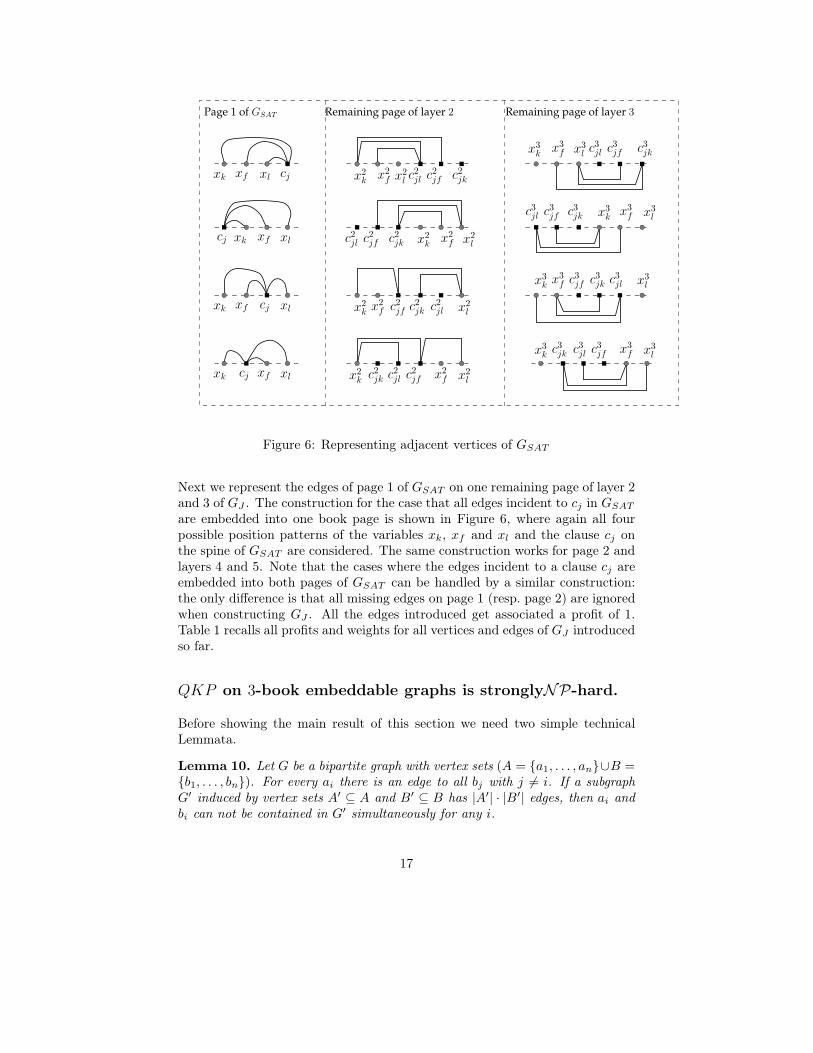
Next we represent the edges of page 1 of GSAT on one remaining page of layer 2and 3 of GJ . The construction for the case that all edges incident to cj in GSAT

are embedded into one book page is shown in Figure 6, where again all fourpossible position patterns of the variables xk, xf and xl and the clause cj onthe spine of GSAT are considered. The same construction works for page 2 andlayers 4 and 5. Note that the cases where the edges incident to a clause cj areembedded into both pages of GSAT can be handled by a similar construction:the only difference is that all missing edges on page 1 (resp. page 2) are ignoredwhen constructing GJ . All the edges introduced get associated a profit of 1.Table 1 recalls all profits and weights for all vertices and edges of GJ introducedso far.

QKP on 3-book embeddable graphs is stronglyNP-hard.

Before showing the main result of this section we need two simple technicalLemmata.

Lemma 10. Let G be a bipartite graph with vertex sets (A = a1, . . . , an∪B =b1, . . . , bn). For every ai there is an edge to all bj with j 6= i. If a subgraphG′ induced by vertex sets A′ ⊆ A and B′ ⊆ B has |A′| · |B′| edges, then ai andbi can not be contained in G′ simultaneously for any i.

17

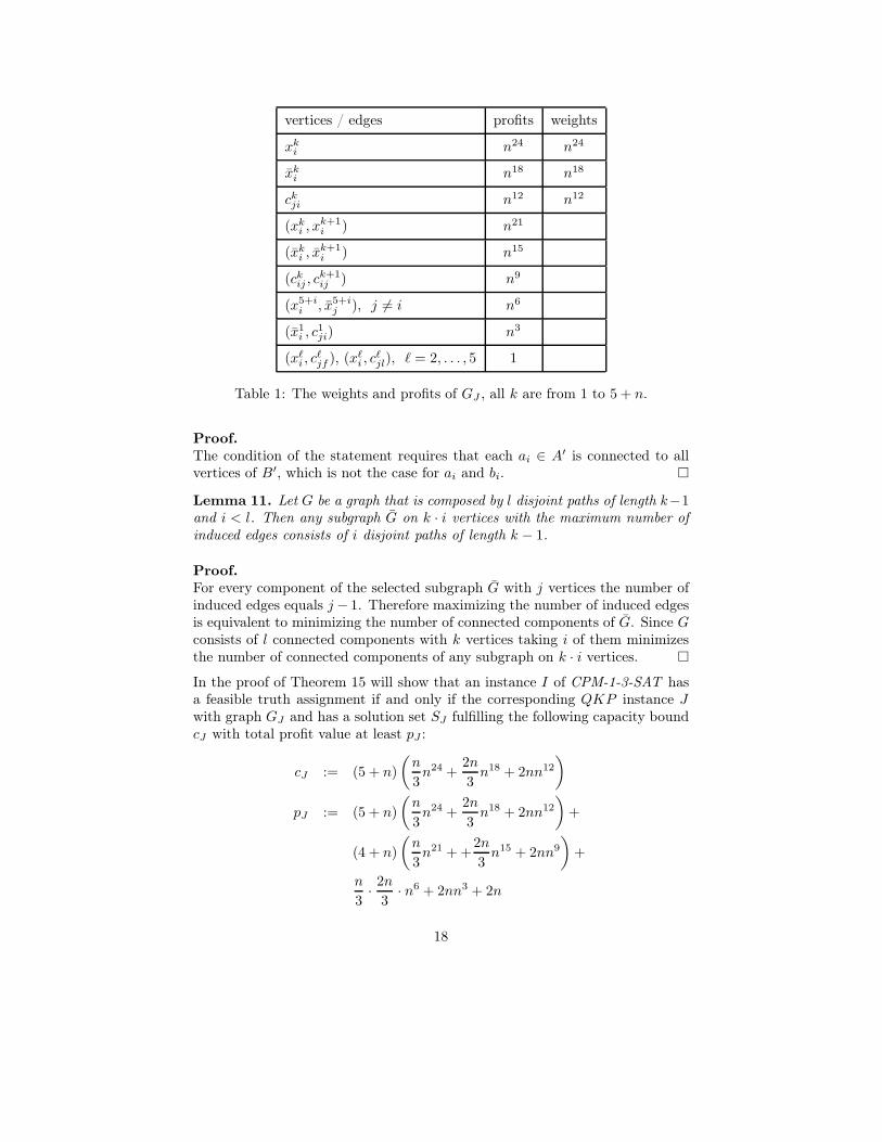
vertices / edges profits weights

xki n24 n24

xki n18 n18

ckji n12 n12

(xki , xk+1

i ) n21

(xki , xk+1

i ) n15

(ckij , c

k+1ij ) n9

(x5+ii , x5+i

j ), j 6= i n6

(x1i , c

1ji) n3

(xℓi , c

ℓjf ), (xℓ

i , cℓjl), ℓ = 2, . . . , 5 1

Table 1: The weights and profits of GJ , all k are from 1 to 5 + n.

Proof.

The condition of the statement requires that each ai ∈ A′ is connected to allvertices of B′, which is not the case for ai and bi.

Lemma 11. Let G be a graph that is composed by l disjoint paths of length k−1and i < l. Then any subgraph G on k · i vertices with the maximum number ofinduced edges consists of i disjoint paths of length k − 1.

Proof.

For every component of the selected subgraph G with j vertices the number ofinduced edges equals j − 1. Therefore maximizing the number of induced edgesis equivalent to minimizing the number of connected components of G. Since Gconsists of l connected components with k vertices taking i of them minimizesthe number of connected components of any subgraph on k · i vertices.

In the proof of Theorem 15 will show that an instance I of CPM-1-3-SAT hasa feasible truth assignment if and only if the corresponding QKP instance Jwith graph GJ and has a solution set SJ fulfilling the following capacity boundcJ with total profit value at least pJ :

cJ := (5 + n)

(

n

3n24 +

2n

3n18 + 2nn12

)

pJ := (5 + n)

(

n

3n24 +

2n

3n18 + 2nn12

)

+

(4 + n)

(

n

3n21 + +

2n

3n15 + 2nn9

)

+

n

3·2n

3· n6 + 2nn3 + 2n

18

Note that the total number of vertices and edges in GJ is of order n2. Therefore,any subset of vertices and edges with profits nk can never reach a total profitof nk+3. This general property of instance J (cf. Table 1) will be exploitedthroughout this section.

The next lemma determines the number of vertices of every type included in afeasible solution SJ . It also guarantees that each of the n + 5 layers of GJ hasthe same structure of included vertices.

Lemma 12. For any feasible solution SJ of a QKP instance J with profitgreater or equal to pJ and weight at most cJ the following structure holds foreach layer k = 1, . . . , n + 5:

1. SJ includes exactly n3 vertices xk

i from each layer k.

2. SJ includes exactly 2n3 vertices xk

i from each layer k.

3. SJ includes exactly 2n vertices ckji from each layer k.

If SJ contains some vertex xki , xk

i or ckji of a layer k, then Sj contains xℓ

i , xℓi

or cℓji for all layers ℓ = 1, . . . , n + 5.

Proof.

We only prove 1. As pointed out above a profit of order n24 can only be obtainedfrom vertices xk

i . To reach pJ , we need (5 + n) · n3 of these, which is also the

maximum number of xki vertices in a feasible solution because of the capacity

constraint.

Therefore, the second largest profit term of order n21 can only be reached byedges (xk

i , xk+1i ). Clearly, these edges in GJ form n disjoint paths of length

n + 4. By Lemma 11 the maximum number of edges induced by any subsetof (5 + n) · n

3 vertices consists of n3 disjoint paths of length n + 4. To reach

the required profit of (4 + n) · n3 n21, we need exactly this maximum number

of edges. For any i, a path of length n + 4 can only occur if all vertices xki

for k = 1, . . . , n + 5 are included in Sj . Moreover, there must be n3 such paths

induced by a vertex xki .

A similar argument can be used to show the remaining points 2. and 3.

Lemma 13. For any feasible solution SJ of a QKP instance J with profitgreater or equal to pJ and weight at most cJ the following holds for each layerk = 1, . . . , 5 + n:

xki ∈ SJ ⇐⇒ xk

i 6∈ SJ

Proof.

It follows from Lemma 12 that all terms of pJ of order at least n9 are contributedby vertices xk

i , xki and ck

ji and the mutual connections of these vertices betweendifferent layers. Analogous to the argument applied in the proof of Lemma 12,profits of order n6 can only be gained by edges (x5+i

i , x5+ij ) j 6= i on layers 5+ i.

19

Merging the vertices xki over all n layers k = 5 + 1, . . . , 5 + n into ai, resp. xk

j

into bj , we get a bipartite graph (A∪B) where ai is connected to bj iff j 6= i. ByLemma 12, SJ induces a subgraph with |A′| = n

3 and |B′| = 2n3 . To reach the

required profit of n3 · 2n

3 · n6 = |A′| · |B′| · n6, Lemma 10 states that SJ can notinduce ai and bi in the subgraph simultaneously. This proves that xk

i and xki

can not be both in SJ . Together with Lemma 12 the statement of the Lemmafollows since at least one of xk

i and xki has to be in SJ .

Lemma 14. For any feasible solution SJ of a QKP instance J with profitgreater or equal to pJ and weight at most cJ the following holds for each layerk = 1, . . . , 5 + n: For every vertex ck

ji in SJ also xki has to be in SJ , whenever

variable xi occurs in clause cj.

Proof.

As before, we note that profit terms of order at least n6 were settled by othervertices and edges. Profit of order n3 are only contributed by edges (x1

i , c1ji).

Lemma 12 states that exactly 2n vertices c1ji are included in SJ . Each of them

is connected to a single vertex x1i by an edge with profit n3.

Therefore, the only way to generate a total profit of 2n ·n3 is the inclusion of allvertices x1

i adjacent to one of the included vertices c1ji. Note that this requires

at least 2n3 vertices x1

i (each of them is connected to three clause vertices) whichis exactly the number of included vertices of that type. By Lemma 12 thestatement is valid also for all layers k > 1.

Theorem 15. QKP defined on 3-book embeddable graphs is strongly NP-hard.

Proof.

Let I be an instance of CPM-1-3-SAT and J the corresponding QKP instanceas defined above. We will show that I has a feasible truth assignment if andonly if instance J has a feasible solution with objective value at least pJ andweight at most cJ .

In Lemma 12 - 14 we identified the structure of a feasible QKP solution im-plied by the profit and weight bounds. In the remainder of the proof we canconcentrate on edges with profit 1 and ignore all other edges.

” ⇐= ”

The profit bound pJ implies that any solution SJ to J contains 2n edges ofprofit 1. By Lemma 12, we know that the same n

3 vertices xki (w.r.t. i) are

chosen from each layer k.

By the construction of GJ (cf. Figure 6) we know that for each i there areexactly 6 neighbors ck

jf connected to xki over all layers k (in fact these are all

found in layers 2, . . . , 5) with an edge of profit 1. Hence all these neighbors haveto be included in SJ to get a total profit of 2n.

We can construct a solution to I as follows: whenever x1i is in SJ , we set xi

to TRUE. We get that I contains exactly n3 variables set to TRUE and that I

20

is a feasible instance: assume that there is a clause cj that has more than onevariable set TRUE (denote them xi and xf ). This means that for some layerk ∈ 2, . . . , 5 also ck

jf is in SJ , since xki is connected to ck

jf . It follows from

Lemma 14 that now also xkf is included in SJ , in contradiction to Lemma 13.

If there is a clause with no variable set TRUE we get by the pigeon-hole principlethat one clause must contain more than one variable set TRUE, again leadingto a contradiction.

” =⇒ ”

Let I be a feasible. If xi is TRUE, include xki in SJ for all layers k, otherwise

include xki and ck

ji in SJ . It is easy to check that SJ is a feasible QKP solutionfulfilling the weight and profit bounds cJ and pJ .

Acknowledgements

The research was funded by the Austrian Science Fund (FWF): P23829-N13

References

N. Alon, S. Arora, R. Manokaran, D. Moshkovitz, and O. Weinstein. Inapprox-imabilty of densest k-subgraph from average case hardness. Technical report,2011.

S. Arora, D. Karger, and M. Karpinski. Polynomial time approximation schemesfor dense instances of NP-hard problems. Journal of Computer and SystemSciences, 58:193–210, 1999.

B.S. Baker. Approximation algorithms for NP-complete problems on planargraphs. Journal of the ACM, 41(1):153–180, 1994.

F. Bernhart and P.C. Kainen. The book thickness of a graph. Journal ofCombinatorial Theory, Series B, 27(3):320 – 331, 1979.

H.L. Bodlaender. A linear-time algorithm for finding tree-decompositions ofsmall treewidth. SIAM Journal on Computing, 25(6):1305–1317, 1996.

H.L. Bodlaender. A partial k-arboretum of graphs with bounded treewidth.Theoretical Computer Science, 209:1–45, 1998.

H.L. Bodlaender and A.M.C.A. Koster. Combinatorial optimization on graphsof bounded treewidth. The Computer Journal, 51(3):255–269, 2008.

D. Chen, R. Fleischer, and J. Li. Densest k-subgraph approximation on intersec-tion graphs. In WAOA ’10: Proceedings of the 8th International Conferenceon Approximation and Online Algorithms, volume 6534 of Lecture Notes inComputer Science, pages 83–93. Springer, 2011.

21

F.R.K. Chung, F.T. Leighton, and A.L. Rosenberg. Embedding graphs in books:a layout problem with applications to VLSI design. SIAM Journal on Alge-braic Discrete Methods, 8(1):33–58, 1987.

D.G. Corneil and Y. Perl. Clustering and domination in perfect graphs. DiscreteApplied Mathematics, 9(1):27 – 39, 1984.

E.D. Demaine, M.T. Hajiaghayi, and K. Kawarabayashi. Algorithmic graphminor theory: Decomposition, approximation, and coloring. In FOCS 2005:Proceedings of the 46th Symposium on Foundations of Computer Science,pages 637 – 646, 2005.

R. Diestel. Graph Theory. Springer, 2006.

U. Feige. Relations between average case complexity and approximation com-plexity. In STOC ’02: Proceedings of the 34th Symposium on Theory ofComputing, pages 534–543. ACM, 2002.

U. Feige, D. Peleg, and G. Kortsarz. The dense k-subgraph problem. Algorith-mica, 29(3):410–421, 2001.

P.C. Kainen and S. Overbay. Book embeddings of graphs and a theorem ofwhitney. Technical report, 2003.

J.M. Keil and T.B. Brecht. The complexity of clustering in planar graphs.Journal of Combinatorial Mathematics and Combinatorial Computing, 9:155–159, 1991.

H. Kellerer and V.A. Strusevich. Fully polynomial approximation schemes fora symmetric quadratic knapsack problem and its scheduling applications. Al-gorithmica, 57:769–795, 2010.

H. Kellerer and V.A. Strusevich. The symmetric quadratic knapsack problem:Approximation and scheduling applications. 4OR, 10:111–161, 2012.

H. Kellerer, U. Pferschy, and D. Pisinger. Knapsack Problems. Springer, 2004.

S. Khot. Ruling out PTAS for graph min-bisection, dense k-subgraph, andbipartite clique. SIAM Journal on Computing, 36(4):1025–1071, 2006.

L. Lovász. Graph minor theory. Bulletin of the American Mathematical Society,43(1):75–86, 2006.

C. Moore and J.M. Robson. Hard tiling problems with simple tiles. Discrete &Computational Geometry, 26(4):573–590, 2001.

T. Nonner. PTAS for densest k-subgraph in interval graphs. In WADS 2011,volume 6844 of Lecture Notes in Computer Science, pages 631–641. Springer,2011.

22

S. Oum and P. Seymour. Approximating clique-width and branch-width. Jour-nal of Combinatorial Theory, Series B, 96:514–528, 2006.

S. Overbay. Graphs with small book thickness. Missouri Journal of Mathemat-ical Sciences, 19(2):121–130, 2007.

U. Pferschy and J. Schauer. The knapsack problem with conflict graphs. Journalof Graph Algorithms and Applications, 13(2):233–249, 2009.

U. Pferschy and J. Schauer. Approximating the quadratic knapsack problemon special graph classes. In WAOA ’13: Proceedings of the 11th Interna-tional Conference on Approximation and Online Algorithms, Lecture Notesin Computer Science. Springer, 2013. to appear.

D. Pisinger. The quadratic knapsack problem - a survey. Discrete AppliedMathematics, 155:623–648, 2007.

D. Pisinger, A.B. Rasmussen, and R. Sandvik. Solution of large quadratic knap-sack problems through aggressive reduction. INFORMS Journal on Comput-ing, 19:280–290, 2007.

D.J. Rader Jr. and G.J. Woeginger. The quadratic 0-1 knapsack problem withseries-parallel support. Operations Research Letters, 30:159–166, 2002.

P. Raghavendra, D. Steurer, and M. Tulsiani. Reductions between expansionproblems. In Electronic Colloquium on Computational Complexity, volumeTR10-172, 2010.

D.J. Rose. On simple characterizations of k-trees. Discrete Mathematics, 7:317–322, 1974.

Z. Xu. A strongly polynomial FPTAS for the symmetric quadratic knapsackproblem. European Journal of Operational Research, 218:377–381, 2012.

M. Yannakakis. Embedding planar graphs in four pages. Journal of Computerand System Sciences, 38:36–67, 1989.

23