Embed Size (px)
Citation preview
Approximation Algorithms for Sequencing Problems
Viswanath Nagarajan
March 2009
Tepper School of BusinessCarnegie Mellon University
Pittsburgh, PA 15213
Thesis Committee:R. Ravi (Chair)
Gerard CornuejolsAnupam GuptaMichael Trick
Submitted in partial fulfillment of the requirements for the degree ofDoctor of Philosophy in Algorithms, Combinatorics and Optimization.

Abstract
This thesis presents approximation algorithms for some sequencingproblems, with an emphasis on vehicle routing. Vehicle Routing Prob-lems (VRPs) form a rich class of variants of the basic Traveling SalesmanProblem, that are also practically motivated. The VRPs considered in thisthesis include single and multiple vehicle Dial a Ride, VRP with StochasticDemands, Directed Orienteering and Directed Minimum Latency. Othersequencing problems studied in this thesis are Permutation FlowshopScheduling and Maximum Quadratic Assignment.

Acknowledgements
I begin by thanking my advisor R. Ravi, who has been a great mentor, colleagueand friend. I am particularly grateful to him for the patience he showed early in mygraduate studies, and for lessons in good research style that I have learnt from him.
I also thank Anupam Gupta, Nikhil Bansal and Maxim Sviridenko, with whomit has been a pleasure collaborating. The downs of failed attempts and the ups ofdiscovering proofs were exciting indeed.
I feel fortunate to have been at CMU along with many other graduate studentswith similar research interests. I thank Dan Golovin, Vineet Goyal, and Mohit Singhfor numerous discussions on research problems (and troubles). I also thank theexcellent faculty members to whom I could turn to for advice: Egon Balas, GerardCornuejols, Alan Frieze, Francois Margot, and Michael Trick.
I would like to thank the Algorithms group at IBM T.J. Watson Research for sum-mer internships in 2007 and 2008, which was a productive and learning experiencefor me. I am also grateful to the financial support I received during my Ph.D. fromthe William Larimer Mellon Fellowship, the Aladdin grant, R. Ravi’s NSF grantsCCR-0430751 and CCF-0728841, and an IBM graduate fellowship.
I also thank my other collaborators not mentioned above, Barbara Anthony,Deeparnab Chakrabarty, Inge Li Gørtz, MohammadTaghi Hajiaghayi, Rohit Khan-dekar, Jochen Konemann, Ravishankar Krishnaswamy, Jon Lee, Aranyak Mehta,Vahab Mirrokni, Britta Peis, Abhiram Ranade, and Vijay Vazirani.
My stay in Pittsburgh has been memorable thanks to my friends Amitabh, John,both Mohits, Prasad, Varun, and Vineet. These years would have seemed a lotlonger without them. I also thank my relatives and friends in the US whom I visitedseveral times during holidays.
I thank my parents and sister for their endless support throughout my Ph.D. I amalso thankful to my parents for instigating in me the value of knowledge, withoutwhich my research motivation would have been incomplete.
v


This thesis is dedicated to my parents.
vii

Contents
1 Introduction 1
1.1 Basics . . . . . . . . . . . . . . . . . . . . . . . . . . . . . . . . . . . 2
1.2 Thesis Contribution and Results . . . . . . . . . . . . . . . . . . . . . 3
1.3 Thesis Outline . . . . . . . . . . . . . . . . . . . . . . . . . . . . . . . 7
2 Single vehicle Dial-a-Ride 9
2.1 Introduction . . . . . . . . . . . . . . . . . . . . . . . . . . . . . . . . 9
2.1.1 The k-Forest Problem . . . . . . . . . . . . . . . . . . . . . . . 10
2.1.2 The Dial-a-Ride Problem . . . . . . . . . . . . . . . . . . . . . 11
2.1.3 Related Work . . . . . . . . . . . . . . . . . . . . . . . . . . . 12
2.2 Algorithms for the k-forest problem . . . . . . . . . . . . . . . . . . . 14
2.2.1 An O(√k) approximation algorithm . . . . . . . . . . . . . . 14
2.2.2 An O(√n) approximation algorithm . . . . . . . . . . . . . . 16
2.2.3 Approximation algorithm for k-forest . . . . . . . . . . . . . . 17
2.3 Applications to Dial-a-Ride problems . . . . . . . . . . . . . . . . . . 18
2.3.1 Classical Dial-a-Ride . . . . . . . . . . . . . . . . . . . . . . . 20
2.3.2 Non-uniform Dial-a-Ride . . . . . . . . . . . . . . . . . . . . . 21
2.3.3 Weighted Dial-a-Ride . . . . . . . . . . . . . . . . . . . . . . . 23
2.4 The Effect of Preemptions . . . . . . . . . . . . . . . . . . . . . . . . 27
3 Multi vehicle Dial-a-Ride 33
ix
x CONTENTS
3.1 Introduction . . . . . . . . . . . . . . . . . . . . . . . . . . . . . . . . 33
3.1.1 Problem Definition and Preliminaries . . . . . . . . . . . . . . 34
3.1.2 Results . . . . . . . . . . . . . . . . . . . . . . . . . . . . . . . 35
3.1.3 Related Work . . . . . . . . . . . . . . . . . . . . . . . . . . . 36
3.2 Uncapacitated Preemptive mDaR . . . . . . . . . . . . . . . . . . . . 37
3.2.1 Reduction to depot-demand instances . . . . . . . . . . . . . 38
3.2.2 Algorithm for depot-demand instances . . . . . . . . . . . . . 39
3.2.3 Tight example for uncapacitated mDaR lower bounds. . . . . 41
3.2.4 Improved guarantee for metrics excluding a fixed minor. . . . 42
3.3 Preemptive multi-vehicle Dial-a-Ride . . . . . . . . . . . . . . . . . . 43
3.3.1 Capacitated Vehicle Routing with Bounded Delay . . . . . . . 44
3.3.2 Algorithm for preemptive mDaR . . . . . . . . . . . . . . . . . 46
3.3.3 Weighted preemptive mDaR . . . . . . . . . . . . . . . . . . . 51
4 Stochastic Demands Vehicle Routing 55
4.1 Introduction . . . . . . . . . . . . . . . . . . . . . . . . . . . . . . . . 55
4.1.1 Results . . . . . . . . . . . . . . . . . . . . . . . . . . . . . . . 56
4.1.2 Related Work . . . . . . . . . . . . . . . . . . . . . . . . . . . 58
4.2 SVRP under Independent Demands . . . . . . . . . . . . . . . . . . . 59
4.3 SVRP under Explicit Demands . . . . . . . . . . . . . . . . . . . . . . 65
4.3.1 Two Auxiliary Problems . . . . . . . . . . . . . . . . . . . . . 67
4.3.2 Algorithm for the Metric Isolation Problem . . . . . . . . . . . 73
4.3.3 Optimal Split Tree Problem . . . . . . . . . . . . . . . . . . . 79
4.3.4 Issue of Observing Demands . . . . . . . . . . . . . . . . . . . 81
4.3.5 Hardness of Approximation . . . . . . . . . . . . . . . . . . . 82
4.4 SVRP under Black-box Distribution . . . . . . . . . . . . . . . . . . . 87
5 VRPs on Asymmetric Metrics 93
5.1 Introduction . . . . . . . . . . . . . . . . . . . . . . . . . . . . . . . . 93
CONTENTS xi
5.1.1 Problem Definition and Preliminaries . . . . . . . . . . . . . . 94
5.1.2 Results . . . . . . . . . . . . . . . . . . . . . . . . . . . . . . . 96
5.1.3 Related Work . . . . . . . . . . . . . . . . . . . . . . . . . . . 96
5.2 Directed k-TSP . . . . . . . . . . . . . . . . . . . . . . . . . . . . . . 97
5.2.1 A linear relaxation for ATSP . . . . . . . . . . . . . . . . . . . 97
5.2.2 Minimum ratio ATSP . . . . . . . . . . . . . . . . . . . . . . . 100
5.2.3 Algorithm for Directed k-TSP . . . . . . . . . . . . . . . . . . 102
5.3 Directed Orienteering . . . . . . . . . . . . . . . . . . . . . . . . . . 103
5.4 Directed Minimum Latency . . . . . . . . . . . . . . . . . . . . . . . 105
5.4.1 Algorithm for directed latency . . . . . . . . . . . . . . . . . . 108
5.4.2 Servicing vertices V1 . . . . . . . . . . . . . . . . . . . . . . . 110
5.4.3 Servicing vertices V2 . . . . . . . . . . . . . . . . . . . . . . . 112
5.4.4 Stitching the local paths . . . . . . . . . . . . . . . . . . . . . 113
5.5 Integrality Gap of ATSP-path . . . . . . . . . . . . . . . . . . . . . . . 113
6 Permutation Flowshop Scheduling 119
6.1 Introduction . . . . . . . . . . . . . . . . . . . . . . . . . . . . . . . . 119
6.1.1 Preliminaries . . . . . . . . . . . . . . . . . . . . . . . . . . . 120
6.1.2 Our Results . . . . . . . . . . . . . . . . . . . . . . . . . . . . 121
6.1.3 Related Work . . . . . . . . . . . . . . . . . . . . . . . . . . . 121
6.2 Randomized Algorithm for Minimizing Makespan . . . . . . . . . . . 123
6.3 A Deterministic Algorithm . . . . . . . . . . . . . . . . . . . . . . . . 126
6.3.1 Properties of the pessimistic estimator . . . . . . . . . . . . . 128
6.3.2 Applying the pessimistic estimators . . . . . . . . . . . . . . . 131
6.4 Weighted sum of completion times . . . . . . . . . . . . . . . . . . . 133
7 Maximum Quadratic Assignment 137
7.1 Introduction . . . . . . . . . . . . . . . . . . . . . . . . . . . . . . . . 137
7.1.1 Our Results . . . . . . . . . . . . . . . . . . . . . . . . . . . . 137
xii CONTENTS
7.1.2 Related Work . . . . . . . . . . . . . . . . . . . . . . . . . . . 138
7.2 General Maximum Quadratic Assignment . . . . . . . . . . . . . . . 139
7.2.1 Algorithm for 0-1 Max-QAP . . . . . . . . . . . . . . . . . . . 141
7.2.2 Maximum Value Common Star Packing . . . . . . . . . . . . . 144
7.2.3 Asymmetric Maximum Quadratic Assignment . . . . . . . . . 147
7.3 Max-QAP under Triangle Inequality . . . . . . . . . . . . . . . . . . 148
7.3.1 Algorithm for the auxiliary problem . . . . . . . . . . . . . . . 149
7.4 Some Remarks on an LP Relaxation for Max-QAP . . . . . . . . . . . 152
8 Conclusions 155
Bibliography 157
List of Figures
3.1 Algorithm UncapMulti for uncapacitated mDaR. . . . . . . . . . . . . 39
3.2 Algorithm for uncapacitated mDaR on Kr-minor free graphs. . . . . . 43
3.3 Cutting and patching steps in algorithm Partial. . . . . . . . . . . . . 50
4.1 An illustration of Step 4 of Partition. . . . . . . . . . . . . . . . . . . . 75
5.1 Linear program (MLP ) for directed latency. . . . . . . . . . . . . . . 109
5.2 Guessed breakpoints v0, · · · , vl and flows sent by the LP betweenconsecutive breakpoints. . . . . . . . . . . . . . . . . . . . . . . . . . 111
7.1 The subgraphs used in random mapping. . . . . . . . . . . . . . . . . 143
xiii

Chapter 1
Introduction
Broadly speaking, a sequencing problem is an optimization problem where feasiblesolutions are specified by a set of orderings on some ground-set. Well-known classesof sequencing problems include machine scheduling, vehicle routing, and assign-ment problems. Due to the complicating nature of constraints in typical sequencingproblems, most of them are NP-complete and hence we do not expect efficient (i.e.polynomial time) exact algorithms. The two main approaches to practical solutionsof such problems are (i) exact algorithms that compute the optimal solution buttake exponential time in the worst case, and (ii) heuristic algorithms that run inpolynomial time but find near-optimal solutions. An approximation algorithm is anefficient heuristic along with a worst-case guarantee on the quality of near-optimalsolutions found by it.
This thesis presents approximation algorithms for a suite of sequencing problems,with emphasis on the class of vehicle routing problems. Vehicle Routing Problems(VRPs) are defined on a set of locations with distances between pairs of locations(also known as metric space), and involve serving a set of client requests using anavailable fleet of vehicles. Examples of client requests are: visiting some set oflocations, moving a set of objects from their source to destination locations etc. Theprecise problem is determined by the nature of these client requests and additionalconstraints on the vehicles. More details on vehicle routing can be found in [151].The most basic VRP is the well-studied Traveling Salesman Problem [131, 7] whichinvolves computing a minimum length tour visiting all locations.
1
2 Chapter 1: Introduction
1.1 Basics
The optimization problems encountered in this thesis have the property that allfeasible solutions have non-negative objective values. An optimization problem isreferred to as a minimization or maximization problem depending on whether thegoal is to minimize or maximize the objective value. An algorithm A for a minimiza-tion (resp. maximization) problem is said to be an α-approximation algorithm if forevery instance I of the problem, A returns a solution with objective value at mostα (resp. at least 1/α) times the optimal value of I. The parameter α is also calledthe approximation guarantee or approximation ratio; α may depend on the inputinstance I, and in this case it is represented as a function α(I). The approximationguarantee α = 1 precisely for an exact algorithm; so the approximation guaranteeof any algorithm is always at least 1.
We define the following three classes of algorithms based on their running timeas a function of the input size n (below c > 0 is any constant).
• Polynomial time: running time is O(nc).
• Quasi-polynomial time: running time is O(2logc n).
• Exponential time: running time is O(2nc).
As is standard, an algorithm is considered efficient if its running time is polynomialin the input size. The P 6= NP conjecture states that NP-complete problems donot admit exact polynomial time algorithms. However even quasi-polynomial timeexact algorithms for NP-complete problems are considered extremely unlikely.
The approximability threshold of an optimization problem refers to the bestachievable approximation ratio for the problem in polynomial time, under suitablecomplexity-theoretic assumptions. For example, the approximability threshhold ofthe minimum k-center problem is two: it admits a 2-approximation algorithm [87],and no better guarantee is possible unless P =NP [89]. Combinatorial optimizationproblems display a wide variety of approximability thresholds, as illustrated in thefollowing.
• Knapsack problem: fully polynomial time approximation scheme (FPTAS) [90],weakly NP-hard.
• Minimum makespan on identical machines: polynomial time approximationscheme (PTAS) [88], strongly NP-hard.
1.2 Thesis Contribution and Results 3
• Max-Coverage: ee−1
(algorithm [120, 37], hardness of approximation [96]).
• Asymmetric k-center: Θ(log∗ n) (algorithm [123], hardness of approxima-tion [35]).
• Set-Cover: lnn (algorithm [93, 108, 36], hardness of approximation [49]).
• Group Steiner tree on trees: O(log2 n)-approximation algorithm [62], Ω(log2−ε n)hardness of approximation for every constant ε > 0 [78].
• Independent Set: trivial n-approximation algorithm, Ω(n1−ε) hardness of ap-proximation for every constant ε > 0 [84].
A finite metric space is represented as a tuple (V, d) where V is a vertex set offinite cardinality (usually denoted |V | = n) and d : V × V → R+ is a distancefunction that satisfies the triangle inequality: d(u, v) + d(v, w) ≥ d(u,w) for allu, v, w ∈ V . The metric is said to be symmetric if d(u, v) = d(v, u) for all u, v ∈ V ;otherwise the metric is called asymmetric. For a symmetric (resp. asymmetric)metric (V, d) and subset S ⊆
(V2
)(resp. S ⊆ V × V ), we define d(S) :=
∑e∈S d(e).
Unless mentioned otherwise, we only deal with symmetric metrics. We also assume(by scaling) that the smallest non-zero distance in any metric is at least one.
1.2 Thesis Contribution and Results
The main focus of this thesis is on Vehicle Routing Problems. The VRPs that weconsider capture various aspects such as capacity constraints, multiple vehicles,transshipment, uncertain demands, and asymmetric distances.
We start with the single vehicle Dial-a-Ride problem in Chapter 2, where a set ofobjects need to be transported from their sources to respective destinations by meansof a single capacitated vehicle. Then we study the Dial-a-Ride problem (Chapter 3)when multiple vehicles are available to move objects and the objective is to minimizethe makespan of the resulting schedule. The setting in multi-vehicle Dial-a-Ridepermits transshipment (also called preemption) of objects at intermediate vertices.On the other hand, the single vehicle Dial-a-Ride problem does not allow transship-ment of objects. The third problem we study, stochastic VRP (Chapter 4), modelsdemand uncertainty in the basic capacitated vehicle routing problem (CVRP). Herethe algorithm only has access to a distribution on the demands, and the true demandat any vertex is observed only when that vertex is visited. In the final chapter on
4 Chapter 1: Introduction
vehicle routing (Chapter 5) we generalize two well-studied VRPs (orienteering andminimum latency problems) to the case where the underlying metric is asymmetric.
A secondary goal in this thesis is the study of other sequencing problems, andin this direction we consider the permutation flowshop scheduling and maximumquadratic assignment problems. Permutation flowshop scheduling (Chapter 6) isa classic machine scheduling problem that involves computing an optimal orderfor jobs to enter a flowshop. Finally, Chapter 7 studies the maximum quadraticassignment problem which is a basic problem in combinatorial optimization general-izing several known problems (eg. traveling salesman, linear arrangement, dense ksubgraph). Given two n× n symmetric non-negative matrices, the objective here isto permute the two matrices so as to maximize the resulting dot-product.
We now describe these problems in some more detail, and state the main resultsobtained. Formal definitions, related work and detailed results appear in the respec-tive chapters. The first four chapters are on vehicle routing.
Single Vehicle Dial a Ride. Chapter 2 studies the basic non-preemptive Dial-a-Rideproblem. Given an n-vertex metric space (V, d), a depot r ∈ V , a set of m demand-pairs (si, ti)mi=1, and a single vehicle of capacity k, the goal is to find a minimumlength tour of the vehicle starting (and ending) at r that moves each object i fromits source si to destination ti such that the vehicle carries at most k objects at anypoint on the tour. It is required that the tour be non-preemptive, i.e. once an objectis picked up from its source, it remains in the vehicle until dropped at its destination.We give an O(
√minn, k · log2 n)-approximation algorithm for this problem, that
improves the previously best known guarantee (in terms of n) of O(√k · log n) [28].
An interesting aspect of our approach is that it also gives similar approximationguarantees for substantially more general cost functions. We also consider the effectof the number of preemptions in single vehicle Dial-a-Ride, and show that for everyDial-a-Ride instance, there is a tour that preempts each object at most once andhas length at most O(log2 n) times the optimal tour that may preempt arbitrarily.On the other hand, even for Dial-a-Ride instances on the Euclidean plane, there isan Ω(n1/8) gap between optimal preemptive and non-preemptive tours. Hence themajor difference in tour-length occurs between zero and one preemption per object.
Multi-Vehicle Dial a Ride. In Chapter 3, we consider the Dial-a-Ride problem withmultiple identical vehicles (i.e. same speed and capacity) where the vehicles mayhave different depot-locations. Here we consider the preemptive version where anobject may be left at intermediate vertices while being transported from source
1.2 Thesis Contribution and Results 5
to destination, and multiple vehicles may be involved in moving the same object.The goal is to compute a schedule of all vehicles that together move objects fromtheir sources to destinations. We give an O(log3 n)-approximation algorithm forminimizing the maximum completion time (a.k.a. makespan) in preemptive multi-vehicle Dial-a-Ride. There is an Ω(log1/4−ε n) hardness of approximation for evenpreemptive single vehicle Dial-a-Ride [67]. We also give improved approximationratios in the following two special cases: when the underlying metric is induced bya graph excluding some fixed minor, and when there is no capacity constraint.
Stochastic Demands VRP. In the stochastic vehicle routing problem (SVRP), asingle vehicle of capacity Q ∈ N is used to distribute units of an identical itemfrom a depot to vertices in an n-vertex metric (V, d), where demands are uncertainand represented by some probability distribution D over 0, 1, · · · , QV . The exactdemand at a vertex is determined only when that vertex is visited. The objective isto compute a strategy of visiting vertices (starting and ending at the depot) suchthat all realized demands are satisfied and the expected tour length is minimized. Wenote that this strategy may be adaptive, i.e. at any point in the tour, the next vertexto visit may depend on the demands observed until then. The complexity of SVRPdepends on the representation of distribution D. The most general setting is wherewe are only given black-box access to the distribution D; however it turns out thatno o(n) approximation ratio is possible in this generality. We consider two naturalways of describing D, that make SVRP more tractable.
• Explicit demand distribution. Here D is specified by m demand scenarios,where each scenario i ∈ [m] specifies demands qiv ∈ 0, 1, · · · , Q at all verticesv ∈ V and the probability pi of its occurrence (where
∑mi=1 pi = 1). We give an
O(log2 n · logm) approximation algorithm in this setting, using a connectionto the group Steiner tree problem [62]. We also show that this problem is atleast as hard to approximate as ‘latency group Steiner tree’, for which O(log2 n)is the best known approximation ratio, and there is an Ω(log1−ε n) hardness ofapproximation [78].
• Independent demand distribution. Here D is specified by means of a de-mand random variable ξv (in the range 0, 1, · · · , Q) at each vertex v ∈ V ,where the random variables ξvv∈V are independent of each other. We obtaina simple randomized approximation algorithm achieving the following worst-case guarantees: (1 + α) under split-delivery VRP (demands can be servedin multiple visits), and (2 + α) for unsplit-delivery VRP (each demand must
6 Chapter 1: Introduction
be served in a single visit); above α denotes the best approximation ratiofor the traveling salesman problem. This result matches (up to an additiveo(1) term) the corresponding best known guarantees for the deterministicversions [5, 6]. Moreover, our algorithm produces an a priori strategy thatalways visits vertices in the same order.
Vehicle Routing on Asymmetric Metrics. We study two vehicle routing problemson asymmetric metrics in Chapter 5. The symmetric counterparts of these problemsare very well-studied and (small) constant factor approximation ratios are known.However, the problems are considerably harder in asymmetric metrics. First we con-sider the directed orienteering problem, that involves computing a bounded-lengthpath from specified origin to destination vertices, visiting the maximum number ofvertices. We provide an O(log2 n)-approximation algorithm for this problem, whichis the first polynomial-time poly-logarithmic approximation guarantee. Combinedwith previously known reductions, this result also implies poly-logarithmic approxi-mation ratios for other directed VRPs such as vehicle routing with time-windows.In the second part of this chapter, we study the directed latency problem: givenan asymmetric metric and a depot vertex, the goal is to compute a tour originat-ing at the depot that minimizes the sum of arrival times at all vertices. This is avariant of the well-known asymmetric traveling salesman problem (ATSP), wherethe objective is minimizing total tour length. We give an LP-based reduction (inquasi-polynomial time) from directed latency to the related asymmetric travelingsalesman path problem (ATSP-path) that implies an O(ρ · log3 n)-approximation algo-rithm for directed latency, where ρ is the integrality gap of a natural LP-relaxation toATSP-path. We conjecture that ρ = O(log n); however the best bound that we obtainhere is ρ = O(
√n). We also show that the directed latency problem is at least as
hard to approximate as ATSP, for which O(log n) is the best known approximationratio.
The last two chapters concern other well-known sequencing problems.
Permutation Flowshop Scheduling. In a flowshop, there are m machines locatedin order 1 through m, and n jobs each of which consists of a sequence of operationson the machines (in the fixed order 1 to m). A permutation schedule involves pro-cessing all jobs subject to the constraint that each machine process all the jobs in thesame order. The goal in permutation flowshop scheduling is to compute a schedule(which corresponds to a permutation on the jobs) that minimizes the completiontime of the last job (i.e. makespan). In Chapter 6 we obtain an O(
√minm,n)-
1.3 Thesis Outline 7
approximation algorithm for the permutation flowshop problem, relative to the triv-ial lower-bounds of maximum job-length and machine-load. This result also boundsthe worst-case gap between permutation and ‘non-permutation’ schedules in theflowshop problem by Θ(
√minm,n); instances showing an Ω(
√minm,n) gap
were known earlier [126]. Furthermore, the algorithm for minimizing makespancan be used to obtain an O(
√minm,n)-approximation algorithm for the weighted
completion time objective, improving substantially over the previously best knownbound of ε ·m (for any constant ε > 0) [144].
Maximum Quadratic Assignment. The input to the quadratic assignment prob-lem [22] consists of two n × n symmetric non-negative matrices W = (wi,j) andD = (di,j). The objective in maximum quadratic assignment (Max-QAP) is to obtaina permutation π : [n] → [n] that maximizes the quantity
∑i,j∈[n],i 6=j wi,j · dπ(i),π(j).
We present an O(√n · log2 n)-approximation algorithm for Max-QAP, which is the
first non-trivial approximation guarantee for this problem. We note that Max-QAPgeneralizes the notorious dense-k-subgraph problem, for which n1/3−δ (here δ > 0 isa small fixed constant) is the best known approximation ratio. We also consider thespecial case when one of the matrices W or D satisfies triangle inequality (i.e. it rep-resents distances in a symmetric metric); in this case we obtain a 2e
e−1-approximation
ratio, improving over the previously best-known bound of four [9].
1.3 Thesis Outline
We now discuss some common threads between different chapters and providean outline for reading this thesis. As mentioned earlier, Chapters 2–5 are onvehicle routing, Chapter 6 is on permutation flowshop scheduling, and Chapter 7is on maximum quadratic assignment. Moreover, Chapters 2–4 deal with VRPs onsymmetric metrics, whereas Chapter 5 deals with asymmetric metrics.
There is a natural progression from Chapter 2 (single vehicle Dial-a-Ride) toChapter 3 (Dial-a-Ride with multiple vehicles). Additionally, some structural proper-ties of Dial-a-Ride tours (from Chapter 2) are used in Chapter 3. It is suggested thatthese two chapters be read in that order. The other chapters are self contained andcan be read independently of each other.
Single vehicle Dial-a-Ride (Chapter 2) and stochastic demands VRP (Chapter 4)both generalize the classic capacitated VRP, albeit in different ways. Dial-a-Ride
8 Chapter 1: Introduction
incorporates multicommodity demands, and SVRP models probabilistic demands.Not surprisingly, the Haimovich-Kan [74] algorithm for capacitated vehicle routingis used/extended in both these chapters.
The main problems of study in Chapter 5 (asymmetric VRPs) are orienteering andminimum latency, in directed graphs. Both these objectives are also encountered inChapter 4, however in the context of the group Steiner tree problem (in symmetricmetrics). Hence the analysis in these two chapters bear some similarity.
The well-known dense-k-subgraph problem is generalized in different ways inChapters 2 and 7. Given an undirected graph G and bound k, dense-k-subgraphinvolves choosing k vertices in G that induce the maximum number of edges. Maxi-mum quadratic assignment (Chapter 7) is a generalization that involves embeddingany arbitrary graph (instead of just the k-clique) onto another so as to maximizethe number of common edges. The main subroutine used in the single vehicle Dial-a-Ride algorithm of Chapter 2 is the k-forest problem, which is another extension ofdense-k-subgraph. In k-forest, the cost of choosing any vertex-subset comes froman arbitrary underlying metric (instead of being the size of this subset).
The permutation flowshop scheduling problem (Chapter 6) and the k-forestproblem (Chapter 2) are both related to increasing subsequences in permutations.This connection is utilized in obtaining algorithms for both these problems. Further-more, the approach used for minimizing weighted completion time in permutationflowshop is similar to that for directed minimum latency (Chapter 5).
Chapter 2
Single vehicle Dial-a-Ride
2.1 Introduction
This chapter studies the single vehicle Dial-a-Ride problem, where given a metricspace with objects having sources and destinations, and a vehicle of some capacityk, the goal is to find a route for this vehicle so that each object can be taken fromits source to destination without exceeding the capacity of the vehicle at any point,such that the length of the vehicle route is minimized. We require that the route benon-preemptive, i.e. once an object is picked up from its source, it remains in thevehicle until delivered to its destination. It turns out that the non-preemptive Dial-a-Ride problem is closely related to a generalization of the Steiner forest problemcalled k-forest, that we now introduce.
In the Steiner forest problem, we are given a set of vertex-pairs in a metric, andthe goal is to find a forest such that each vertex-pair is connected in the forest. Thisis a generalization of the Steiner tree problem, where all the pairs contain a commonvertex called the root; both the tree and forest versions are well-understood funda-mental problems in network design, and constant factor approximation algorithmsare known [132, 4, 69]. An important extension of the Steiner tree problem studiedin the late 1990s was the k-MST problem, where one sought the least-cost tree thatconnected any k of the terminals: several approximation algorithms were givenfor the problem, culminating in the 2-approximation of [64]. The k-MST problemproved crucial in many subsequent developments in network design and vehiclerouting [29, 45, 17, 13]. One can analogously define the k-forest problem whereone needs to connect only k of the pairs in some Steiner forest instance: surprisingly,
9
10 Chapter 2: Single vehicle Dial-a-Ride
very little is known about this problem, which was first studied formally only re-cently [75, 140]. We give simpler and improved approximation algorithms for thek-forest problem, and show how this implies good approximation bounds for theDial-a-Ride problem.
2.1.1 The k-Forest Problem
Our starting point is the k-forest problem.
Definition 1. Given an n-vertex metric space (V, d), and demand pairs si, timi=1 ⊆V × V , find the least-cost subgraph that connects at least k pairs.
We note that demand pairs may be repeated; so k and m may be super-polynomial in n. The k-forest problem is also a generalization of the (minimiza-tion version of the) well-studied dense-k-subgraph problem, where given a graphG = (V,E) and a target k ≤ |E|, the goal is to compute a minimum cardinality sub-set U ⊆ V of vertices that induce at least k edges. Despite several attempts, nothingbetter than an O(n1/3−δ)-approximation is known for dense-k-subgraph (δ > 0 issome fixed constant); improving upon this is a long-standing open question. Thek-forest problem was first defined in [75], and the first non-trivial approximationwas given by [140], who gave an algorithm with an approximation guarantee ofO(minn2/3,
√m log n). We obtain the following improved approximation guaran-
tee for k-forest in Section 2.2.
Theorem 2. There is an O(min√n · log k,√k)-approximation algorithm for the
k-forest problem.
The proof of this theorem involves two algorithms, both reducing the k-forestproblem to the k-MST problem in different ways and achieving different approxima-tion guarantees. The first algorithm (giving an approximation of O(
√k)) uses the
k-MST algorithm to find good solutions on the sources and the sinks independently,and then uses the Erdos-Szekeres theorem on monotone subsequences to find a“good” subset of these sources and sinks to connect cheaply; details are given inSection 2.2.1. The second algorithm starts off with a single vertex as the initialsolution, and uses the k-MST algorithm to repeatedly find a low-cost tree thatsatisfies a large number of pairs having one endpoint in the current solution andthe other endpoint outside; this tree is then used to greedily augment the currentsolution and proceed. Choosing the parameters (as described in Section 2.2.2) givesus an O(
√n) approximation.
2.1 Introduction 11
2.1.2 The Dial-a-Ride Problem
The Dial-a-Ride problem is formally defined as follows.
Definition 3. Given an n-vertex metric space (V, d), a starting vertex (or root) r, a setof m objects with source-destination pairs (si, ti)mi=1, and a vehicle of capacity k, finda minimum length tour of the vehicle starting (and ending) at r that moves each objecti from its source si to its destination ti such that the vehicle carries at most k objects atany point on the tour.
Each demand-pair in the Dial-a-Ride problem corresponds to an object that isto be moved from the specified source to destination. We use the terms: demand-pair, object, and pair interchangeably. In the preemptive Dial-a-Ride problem, afterpicking up an object from its source, it may be left at some intermediate verticesbefore being delivered to its destination. In this paper we will mainly be concernedwith the non-preemptive Dial-a-Ride problem, where once an object is picked upfrom its source, it remains in the vehicle until dropped at its destination. A note onthe parameters: using triangle inequality, any feasible non-preemptive tour can beshort-cut over vertices that do not participate in any demand-pair; hence we canassume that every vertex is an end point of some demand-pair, i.e. n ≤ 2m. Again,we allow multiple demand-pairs between the same pair of vertices; so the numberof objects m and the vehicle capacity k may be larger than any polynomial in n.
We now mention two lower bounds for the preemptive Dial-a-Ride problemthat are used in Chapters 2 and 3. The Steiner lower bound is the minimum lengthTSP tour on the set of all sources and destinations; and the flow lower boundequals
∑mi=1
d(si,ti)k
. Note that for any Dial-a-Ride instance, the cost of an optimalpreemptive tour is at most that of an optimal non-preemptive tour.
The approximability of the non-preemptive Dial-a-Ride problem is not verywell understood: the previous best upper bound is an O(
√k log n)-approximation
algorithm due to [28], whereas the best lower bound that we are aware of is APX-hardness. We establish the following (somewhat surprising) connection betweenthe Dial-a-Ride and k-forest problems in Section 2.3.
Theorem 4. Given an α-approximation algorithm for k-forest, there is an O(α · log2 n)-approximation algorithm for the Dial-a-Ride problem.
In particular, combining Theorems 2 and 4 gives us an O(min√k,√n · log2 n)-
approximation guarantee for Dial-a-Ride. Of course, improving the approximationguarantee for k-forest would improve the result for Dial-a-Ride as well.
12 Chapter 2: Single vehicle Dial-a-Ride
Our results match the previous best bound up to a logarithmic term, and givean improvement when the vehicle capacity k n, the number of nodes. Moreinterestingly, our algorithm for Dial-a-Ride easily extends to generalizations ofthe Dial-a-Ride problem. In particular, we consider a substantially more generalvehicle routing problem where the vehicle has no a priori capacity, and insteadthe cost of traversing each edge e is an arbitrary non-decreasing function ce(l) ofthe number of objects l in the vehicle; setting ce(l) to the edge-length de whenl ≤ k, and ce(l) = ∞ for l > k gives us back the classical Dial-a-Ride setting. InSection 2.3.2, we show that this general non-uniform Dial-a-Ride problem admitsan O(
√n · log2m) approximation guarantee. Another extension we consider is the
weighted Dial-a-Ride problem. In this, each object may have a different size, and thetotal size of the items in the vehicle must be bounded by the vehicle capacity; this isalso known as the pickup and delivery problem [135]. We show in Section 2.3.3 thatthis problem can be reduced to the (unweighted) Dial-a-Ride problem at the lossof only a constant factor in the approximation guarantee: so weighted Dial-a-Rideadmits an O(
√n log2 n)-approximation algorithm.
We also consider the effect of preemptions in the Dial-a-Ride problem (Sec-tion 2.4). It was shown in [28] that the gap between the optimal preemptive andnon-preemptive tours could be as large as Ω(n1/3). We show that the real differencearises between zero and one preemptions: allowing multiple preemptions doesnot give us much added power. In particular, we show in Section 2.4 that for anyinstance of the Dial-a-Ride problem, there is a tour that preempts each object at mostonce and has length at most O(log2 n) times an optimal preemptive tour (which maypreempt each object an arbitrary number of times). Motivated by obtaining a betterguarantee for Dial-a-Ride on the Euclidean plane, we study the preemption gap insuch instances. We show that even in this case, there are instances having an Ω(n1/8)gap between optimal preemptive and non-preemptive tours. This preemption gaprelies on the connection between the Dial-a-Ride and k-forest.
2.1.3 Related Work
The k-forest problem: The k-forest problem is relatively new: it was defined by[75]. An O(k2/3)-approximation algorithm for even the directed k-forest problemcan be inferred from [27]. Recently, [140] gave an O(minn2/3,
√m log n) approx-
imation algorithm for k-forest. The k-forest problem is a generalization of k-MST,for which a 2-approximation is known [64].
2.1 Introduction 13
Dense k-subgraph: As shown in [75], the k-forest problem also generalizes thedense-k-subgraph problem [52]. The best known approximation guarantee forthe dense-k-subgraph problem is O(n1/3−δ) where δ > 0 is some constant, due to[52], and obtaining an improved guarantee has been a long standing open prob-lem. Strictly speaking, [52] study a potentially harder problem: the maximizationversion of dense-k-subgraph, where one wants to pick k vertices to maximize thenumber of edges in the induced graph. However, nothing better is known evenfor the minimization version of dense-k-subgraph (where one wants to pick theminimum number of vertices that induce k edges). Moreover, the approximabilityof these two versions of dense-k-subgraph are polynomially related [75]. The mini-mization dense-k-subgraph problem on graph G reduces to k-forest by consideringan unweighted star-metric, with leaves corresponding to vertices of G and pairscorresponding to edges of G.
Dial-a-Ride: Dial-a-Ride problems form an interesting subclass of Vehicle RoutingProblems that are well studied in the operations research literature. Savelsberg andSol [135] and Cordeau and Laporte [39] survey several variants of non-preemptiveDial-a-Ride problems that have been studied in the literature.
While the Dial-a-Ride problem has been studied extensively in the operationsresearch literature, relatively little is known about its approximability. The currentlybest known approximation ratio for non-preemptive Dial-a-Ride is O(
√k log n) due
to [28]. We note that their algorithm assumes instances with unweighted objects.[102] give a 3-approximation algorithm for the Dial-a-Ride problem on a line metric;in fact, their algorithm finds a non-preemptive tour that has length at most 3 timesthe lower bounds for the preemptive version. A 2.5-approximation algorithm forsingle source special case of Dial-a-Ride (also called the capacitated vehicle routingproblem) was given in [74]; again, this algorithm outputs a non-preemptive tourwith length at most 2.5 times the preemptive lower bounds. The k = 1 specialcase of Dial-a-Ride is also known as the stacker-crane problem, for which a 1.8-approximation is known [58]. For the preemptive Dial-a-Ride problem, [28] gavethe current-best O(log n) approximation algorithm, and [67] showed that it isΩ(log1/4−ε n) hard to approximate. Recall that no super-constant hardness resultsare known for the non-preemptive Dial-a-Ride problem.
14 Chapter 2: Single vehicle Dial-a-Ride
2.2 Algorithms for the k-forest problem
In this section, we study the k-forest problem, and give an approximation guaranteeofO(min√n,
√k). Our approach is based on approximating the following “density”
variant of k-forest.
Definition 5. Minimum-ratio k-forest. Given an n-vertex metric space (V, d), mpairs of vertices si, timi=1, and a target k, find a tree T that connects at most k pairs,and minimizes the ratio of the length of T to the number of pairs connected in T .
Observe that given any forest F connecting some set of pairs, one of the trees inF has ratio (length to number of connected pairs) at most that of F . Hence even ifwe relax the above definition to consider any forest, the optimal ratio solution canbe assumed to be a tree. Given any feasible solution T to minimum-ratio k-forest,Ratio(T ) denotes the ratio of length of T to the number of pairs connected in T .
We present two different algorithms for minimum-ratio k-forest, obtaining ap-proximation guarantees of O(
√k) (Section 2.2.1) and O(
√n) (Section 2.2.2); these
are then combined to give the claimed result for the k-forest problem. Both ouralgorithms are based on reductions to the k-MST problem, albeit in very differentways. As is usual, when we say that our algorithm guesses a parameter in thefollowing discussion, it means that the algorithm is run for each possible value ofthat parameter, and the best solution found over all the runs is returned. As longas only a constant number of parameters are being guessed and the number ofpossibilities for each of these parameters is polynomial, the algorithm is repeatedonly a polynomial number of times.
2.2.1 An O(√k) approximation algorithm
In this section, we give an O(√k) approximation algorithm for minimum ratio
k-forest, which is based on a simple reduction to the k-MST problem. The idea isto look at the optimal solution S to minimum-ratio k-forest and consider an Eulertour of this tree S—a theorem of Erdos and Szekeres on increasing subsequencesimplies that there must be at least
√|S| sources which are visited in the same order
as the corresponding sinks. We use this existence result to combine the source-sinkpairs to create an instance of
√|S|-MST from which we can obtain a good solution;
the details follow. Below S denotes an optimal ratio tree, that covers q pairs andhas length B; let D denote the largest distance between any demand-pair that iscovered in S (note D ≤ B).
2.2 Algorithms for the k-forest problem 15
The O(√k) approximation algorithm proceeds as below. Define a new metric
l on the set 1, · · · ,m of pairs as follows. The distance between pairs i and j,li,j
.= d(si, sj) + d(ti, tj), where (V, d) is the original metric. This metric represents
solutions of a special structure: any tree M covering pairs Π can be expressed asM = Ms ∪Mt ∪ f where Ms (resp. Mt) is a tree connecting all sources (resp.destinations) in Π and f is any edge connecting a pair in Π. The algorithm guessesthe number of pairs q and the largest demand-pair distance D in the optimal treeS (there are at most m choices for each of q and D). The algorithm discards allpairs (si, ti) such that d(si, ti) > D (all the pairs covered in the optimal solution Sstill remain). Then the algorithm runs the unrooted k-MST algorithm [64] withtarget b√qc, in the metric l, to obtain a tree T on the pairs P . From T , we easilyobtain trees T1 (on all sources in P ) and T2 (on all sinks in P ) in metric d suchthat d(T1) + d(T2) = l(T ). Finally the algorithm outputs the tree T ′ = T1 ∪ T2 ∪ e,where e is any edge joining a source in T1 to its corresponding sink in T2.
Due to the pruning on pairs that have large distance, d(e) ≤ D and the lengthof T ′, d(T ′) ≤ l(T ) + D ≤ l(T ) + B. We now argue that the cost of the solution Tfound by the k-MST algorithm l(T ) ≤ 8B. Consider the optimal ratio tree S (inmetric d) that has q pairs (s1, t1), · · · , (sq, tq), and let τ denote an Euler tour ofS. Suppose that in a traversal of τ , the sources of pairs in S are seen in the orders1, · · · , sq. Then in the same traversal, the sinks of pairs in S will be seen in theorder tπ(1), · · · , tπ(q), for some permutation π. The following fact is well known (see,e.g., [146]).
Theorem 6. (Erdos and Szekeres) Every permutation on 1, · · · , q has either anincreasing subsequence of length b√qc or a decreasing subsequence of length b√qc.
Using Theorem 6, we obtain a set M of p = b√qc pairs such that (1) thesources in M appear in increasing order in a traversal of the Euler tour τ , and(2) the sinks in M appear in increasing order in a traversal of either τ or τR
(the reverse traversal of τ). Let j0 < j1 < · · · < jp−1 denote the pairs in M inincreasing order. From statement (1) above,
∑p−1i=0 d(s(ji), s(ji+1)) ≤ d(τ), where
the indices in the summation are modulo p. Similarly, statement (2) implies that∑p−1i=0 d(t(ji), t(ji+1)) ≤ maxd(τ), d(τR) = d(τ). Thus we obtain:
p−1∑i=0
[d(s(ji), s(ji+1)) + d(t(ji), t(ji+1))] ≤ 2d(τ) ≤ 4B
But this sum is precisely the length of the tour j0, j1, · · · , jp−1, j0 in metric l. In otherwords, there is a tree of length 4B in metric l, that contains b√qc vertices. So, thecost of the solution T found by the k-MST approximation algorithm is at most 8B.
16 Chapter 2: Single vehicle Dial-a-Ride
Now the final solution T ′ has length at most l(T ) + B ≤ 9B, and Ratio(T ′) ≤9√qBq≤ 9√kBq. Thus we have an O(
√k) approximation algorithm for minimum
ratio k-forest.
2.2.2 An O(√n) approximation algorithm
In this section, we show an O(√n) approximation algorithm for the minimum ratio
k-forest problem. The approach is again to reduce to the k-MST problem; the idea israther different: either we find a vertex v such that a large number of demand-pairsof the form (v, ∗) can be satisfied using a small tree (the “high-degree” case), or weuse a repeated greedy procedure to cover most vertices without paying too much(since we are in the “low-degree” case, covering most vertices implies covering mostpairs too). The details follow.
Let S denote an optimal solution to minimum ratio k-forest, and q ≤ k thenumber of demand pairs covered in S. We define the degree ∆ of S to be themaximum number of demand-pairs (among those covered in S) that are incidentat any vertex in S. The algorithm first guesses the following parameters of theoptimal solution S: its length B (within a factor 2), the number of pairs coveredq, the degree ∆, and the vertex w ∈ S that has ∆ demand-pairs incident at it.Although, there may be an exponential number of choices for the optimal length, apolynomial number of guesses within a binary-search suffice to get a B such thatB ≤ d(S) ≤ 2 · B. The algorithm then returns the better of the two proceduresdescribed below.
Procedure 1 (high-degree case): The algorithm assigns a weight to each vertex u,equal to the number of pairs having an end point at u and the other end point at w(the guessed ∆-degree vertex in S). Then we run the k-MST algorithm [64] withroot w and a target weight of ∆, resulting in a solution tree H. Since the degree ofvertex w in the optimal solution S is ∆, there is tree rooted at w of length d(S) ≤ 2B,that contains at least ∆ pairs having one end point at w. Hence the k-MST instancehas a feasible solution of length 2B, and the length of solution H is at most 4B(since the algorithm of [64] is a 2-approximation). Thus Ratio(H) ≤ 4B/∆ = 4q
∆Bq.
Procedure 2 (low-degree case): Set t = q2∆
; note that q ≤ ∆·n2
and so t ≤ n/4. Wemaintain a current tree T (which is initialized to T ← w), and iteratively do thefollowing:
1. Shrink T to a single vertex s in metric (V, d), and run the k-MST algorithm [64]
2.2 Algorithms for the k-forest problem 17
with root s and a target of t new vertices. Let T0 denote the resulting tree.
2. If T0 has length at most 4B, set T ← T ∪ T0 and continue to the next iteration.
3. If T0 has length more than 4B (or if T already has all vertices) then terminate.
The tree T at the end of these iterations is output as the solution to minimumratio k-forest. Since t new vertices are added in each iteration, the number ofiterations is at most n
t; so the length of T is at most 4n
tB. We now show that T
contains at least q2
demand-pairs. Consider the set S \ T (recall, S is the optimalsolution). It is clear that |V (S) \V (T )| < t; otherwise the k-MST instance in the lastiteration (with the current T ) would have S as a feasible solution of length at most2B (and hence would find one of length at most 4B). So the number of pairs coveredin S that have at least one end point in S\T is at most |V (S)\V (T )| ·∆ ≤ t ·∆ = q/2(as ∆ is the degree of solution S). Thus there are at least q/2 pairs contained inS ∩ T , in particular in T . Thus T is a solution with Ratio(T ) ≤ 4n
tB · 2
q= 8n
tBq.
The better solution among H and T from the above two procedures has objectivevalue at most min4q
∆, 8nt · B
q= min8t, 8n
t · B
q≤ 8√n · B
q≤ 8√n · d(S)
q. So this
algorithm is an O(√n) approximation to the minimum ratio k-forest problem.
2.2.3 Approximation algorithm for k-forest
Given the two algorithms for minimum ratio k-forest, we can use them in a standardgreedy fashion (i.e., keep picking approximately minimum-ratio solutions until weobtain a forest connecting at least k pairs); the standard set cover analysis can beused to show an O(min√n,
√k · log k)-approximation guarantee for k-forest. The
O(√k · log k) part of the bound can be improved slightly to O(
√k). This uses a
tighter analysis of the greedy set-cover algorithm [27]. Lemma 1 from [27] impliesthe following in our context: Suppose there is an f(k) approximation algorithmfor minimum ratio k-forest, where f(x)/x is a decreasing function of x. Then thegreedy algorithm for the k-forest problem achieves an approximation guarantee of∫ k
0f(x)/x dx. Using f(k) = O(
√k), we obtain an O(
√k) approximation for k-forest,
implying the guarantee in Theorem 2.
We note that this greedy approach to solving the k-forest problem may not evengive an o(n) approximation bound when k is super-polynomial in n. In this casehowever, our O(
√n)-approximation algorithm for minimum ratio k-forest can be
used within the Lagrangian relaxation framework of [140] (in place of Theorem 3)to obtain an O(
√n · log n) approximation for k-forest.
18 Chapter 2: Single vehicle Dial-a-Ride
2.3 Applications to Dial-a-Ride problems
In this section, we study applications of k-forest to the Dial-a-Ride problem (Def-inition 3), and some generalizations. A natural solution-structure for Dial-a-Rideinvolves servicing objects in batches of at most k each, where a batch consisting of aset S of demand-pairs is served as follows: the vehicle starts out being empty, picksup each of the |S| ≤ k objects from their sources, then drops off each object at itsdestination, and is again empty at the end. If we knew that the optimal solution hasthis structure, we could obtain a greedy framework for Dial-a-Ride by repeatedlyfinding the best ‘batch’ of k demand-pairs. However, the optimal solution mayinvolve carrying almost k objects at every point in the tour, in which case it can notbe decomposed to be of the above structure. In Theorem 7, we show that there isalways a near optimal solution having this ‘pick-drop in batches’ structure. Buildingon Theorem 7, we obtain approximation algorithms for the classical Dial-a-Rideproblem (Section 2.3.1), and two interesting extensions: non-uniform Dial-a-Ride(Section 2.3.2) and weighted Dial-a-Ride (Section 2.3.3).
Theorem 7. Given any instance of Dial-a-Ride, there exists a feasible tour τ satisfyingthe following conditions:
1. τ can be split into a set of segments S1, · · · , St (i.e., τ = S1 · S2 · · ·St) whereeach segment Si services a set Oi of at most k objects such that Si is a path thatfirst picks up each object in Oi and then drops each of them.
2. The length of τ is at most O(logm) times the length of an optimal tour.
Proof: Consider an optimal non-preemptive tour σ: let d(σ) denote its length, and|σ| denote the number of edge traversals in σ. Note that if in some visit to a vertex vin σ there is no pick-up or drop-off, then the tour can be short-cut over vertex v, andit still remains feasible. Further, due to triangle inequality, the length d(σ) does notincrease by this operation. So we may assume that each vertex visit in σ involves apick-up or drop-off of some object. Since there is exactly one pick-up and drop-offfor each object, we have |σ| ≤ 2m+ 1. Define the stretch of a demand-pair i to bethe number of edge traversals in σ between the pick-up and drop-off of object i.The demand-pairs are partitioned as follows: for each j = 1, · · · , dlog(2m)e, groupGj consists of all pairs having stretch between 2j−1 and 2j. We consider each groupGj separately.
Claim 8. For each j = 1, · · · , dlog(2m)e, there is a tour τj that serves all the pairs ingroup Gj, satisfies condition 1 of Theorem 7, and has length at most 6 · d(σ).
2.3 Applications to Dial-a-Ride problems 19
Proof: Consider tour σ as a line L, with every edge traversal in σ represented bya distinct edge in L. Number the vertices in L from 0 to h, where h = |σ| is thenumber of edge traversals in σ. Note that each vertex in V may be representedmultiple times in L. Each object is associated with the numbers of the vertices (inL) where it is picked up and dropped off.
Let r = 2j−1, and partition Gj as follows: for l = 1, · · · , dhre, set Ol,j consists
of all objects in Gj that are picked up at a vertex numbered between (l − 1)r andlr − 1. Since every object in Gj has stretch in the interval [r, 2r], every object in Ol,j
is dropped off at a vertex numbered between lr and (l + 2)r − 1. Note that |Ol,j|equals the number of objects in Gj carried over edge (lr − 1, lr) by tour σ, which isat most k. We define segment Sl,j to start at vertex number (l − 1)r and traverse alledges in L until vertex number (l + 2)r − 1 (servicing all demand-pairs in Ol,j byfirst picking up each object between vertices (l − 1)r and lr − 1; then dropping offeach object between vertices lr and (l + 2)r − 1), and then return (with the vehiclebeing empty) to vertex lr. Clearly, the number of objects carried over any edge inSl,j is at most the number carried over the corresponding edge traversal in σ. Also,each edge in L participates in at most 3 segments Sl,j | 1 ≤ l ≤ dh/re, and eachedge is traversed at most twice in any segment. So the total length of all segmentsSl,j is at most 6 · d(σ). We define tour τj to be the concatenation S1,j · · ·Sdh/re,j. Itis clear that this tour satisfies condition 1 of Theorem 7.
Applying this claim to each group Gj, and concatenating the resulting tours, weobtain the tour τ satisfying condition 1 and having length at most 6 log(2m) · d(σ) =O(logm) · d(σ).
Remark: The ratio O(logm) in Theorem 7 is almost best possible. As mentioned in[66], there are instances of Dial-a-Ride on an unweighted line, where every solutionsatisfying condition 1 of Theorem 7 has length at least Ω(max logm
log logm, k
log k) times
the optimal non-preemptive tour. These instances consist of n = 2k + 1 equallyspaced vertices on a line, numbered 1 through n+ 1 from left to right, with demand-pairs (j ·2i, (j+ 1)2i) | 0 ≤ i ≤ k, 0 ≤ j ≤ 2k−i−1. It can be seen that the optimalnon-preemptive tour has length O(n), whereas any tour satisfying condition 1 ofTheorem 7 has length at least Ω(n · logn
log logn). So, if we only use solutions of this
‘pick-drop’ structure, then it is not possible to obtain an approximation factor (justin terms of capacity k) for Dial-a-Ride that is better than Ω(k/ log k). The solutionsfound by the algorithm for Dial-a-Ride in [28] also satisfy condition 1 of Theorem 7.It is interesting to note that when the underlying metric is a hierarchically well-separated tree (HST), [28] obtain a solution of such structure having length O(
√k)
times the optimum, whereas there is a lower bound of Ω( klog k
) even for the simple
20 Chapter 2: Single vehicle Dial-a-Ride
case of an unweighted line (which is not an HST).
2.3.1 Classical Dial-a-Ride
Theorem 7 suggests a greedy strategy for Dial-a-Ride, based on repeatedly findingthe best batch of k objects to service. This greedy subproblem turns out to bethe minimum ratio k-forest problem (Definition 5), for which we already have anapproximation algorithm. The next theorem sets up this reduction.
Theorem 9. A ρ-approximation algorithm for minimum ratio k-forest implies anO(ρ log2m)-approximation algorithm for Dial-a-Ride.
Proof: The algorithm for Dial-a-Ride is as follows.
1. C = φ.
2. Until there are no uncovered demand-pairs, do:
(a) Solve the minimum ratio k-forest problem, to obtain a tree C covering kC ≤ knew pairs.
(b) Set C ← C ∪ C.
3. For each tree C ∈ C, obtain an Euler tour on C to locally service all demand-pairs(pick up all kC objects in the first traversal, and drop them all in the second traversal).Then use a 1.5-approximate TSP tour on the sources, to connect all the local tours,and obtain a feasible non-preemptive tour.
Consider the tour τ and its segments as in Theorem 7. If the number of uncoveredpairs in some iteration is m′, one of the segments in τ is a solution to the minimumratio k-forest problem of value at most d(τ)
m′. Since we have a ρ-approximation
algorithm for this problem, we would find a segment of ratio at most O(ρ) · d(τ)m′
.Now a standard set cover type argument shows that the total length of trees in Cis at most O(ρ logm) · d(τ) ≤ O(ρ log2m) · OPT, where OPT is the optimal value ofthe Dial-a-Ride instance. Further, the TSP tour on all sources is a lower bound onOPT, and we use a 1.5-approximate solution [34]. So the final non-preemptive touroutput in step 5 above has length at most O(ρ log2m) · OPT.
This theorem is in fact stronger than Theorem 4 claimed earlier: any approx-imation algorithm for k-forest implies an algorithm with the same guarantee forminimum ratio k-forest. Note that, m and k may be super-polynomial in n. However,
2.3 Applications to Dial-a-Ride problems 21
we show in Section 2.3.3 that with the loss of a constant factor, even the weightedDial-a-Ride problem can be reduced to classical Dial-a-Ride where the number ofobjects m ≤ n4. Based on this and Theorem 9, a ρ approximation algorithm forminimum ratio k-forest actually implies an O(ρ log2 n) approximation algorithmfor Dial-a-Ride. Using the approximation algorithm for minimum ratio k-forest(Section 2.2), we obtain an O(min√n,
√k · log2 n) approximation algorithm for
the Dial-a-Ride problem.
Remark: If we use the O(√k) approximation for k-forest, the resulting non-
preemptive tour is in fact feasible even for a√k capacity vehicle! As noted in
[28], this property is also true of their algorithm, which is based on an entirelydifferent approach.
2.3.2 Non-uniform Dial-a-Ride
The greedy framework for Dial-a-Ride described above is actually more generallyapplicable than to just the classical Dial-a-Ride problem. In this section, we considerthe Dial-a-Ride problem under a substantially more general class of cost functions,and show how the k-forest problem can be used to obtain an approximation al-gorithm for this generalization as well. In fact, the approximation guarantee weobtain by this approach matches (up to logarithmic factors) the best known forthe classical Dial-a-Ride problem. Our framework for Dial-a-Ride is well suited forsuch a generalization since it is based on directly approximating a near-optimalsolution; this approach is not too sensitive to the cost function. On the other hand,the algorithm in [28] is based on obtaining a good lower bound, which dependsheavily on the cost function. Thus it is unclear whether their techniques can beextended to handle such a generalization.
Definition 10. Non-uniform Dial-a-Ride. Given an n vertex undirected graph G =(V,E), a root vertex r, a set of m demand-pairs (si, ti)mi=1, and a non-decreasing costfunction ce : 0, 1, · · · ,m → R+ on each edge e ∈ E (where ce(l) is the cost incurredby the vehicle in traversing edge e while carrying l objects), find a non-preemptive tour(starting and ending at r) of minimum total cost that moves each object i from si to ti.
Note that the classical Dial-a-Ride problem is a special case when the edge costsare given by: ce(l) = de if l ≤ k and ce(l) = ∞ otherwise, where de is the edgelength in the underlying metric. We may assume (without loss in generality) thatfor any fixed value l ∈ [0,m], the edge costs ce(l) induce a metric on V . Similar to
22 Chapter 2: Single vehicle Dial-a-Ride
Theorem 7, we have a near optimal solution with a ‘batch’ structure for the non-uniform Dial-a-Ride problem as well, which implies the algorithm in Theorem 12.
Corollary 11. Given any instance of non-uniform Dial-a-Ride, there exists a feasibletour τ satisfying the following conditions:
1. τ can be split into a set of segments S1, · · · , St (i.e., τ = S1 · S2 · · ·St) whereeach segment Si services a set Oi of demand-pairs such that Si is a path that firstpicks up each object in Oi and then drops each of them.
2. The cost of τ is at most O(logm) times the cost of an optimal tour.
Proof: We only give a proof sketch highlighting how the proof of Theorem 7 carriesover to this case. We may again assume that the number of edge traversals in the anoptimal tour σ is at most 2m: this uses triangle inequality in the edge-costs ce(l) forany fixed l ∈ [m]. The definitions of groups Gj | j = 1, · · · , dlog(2m)e, and Ol.jfor each 1 ≤ j ≤ dlog(2m)e are identical to those in Theorem 7. The traversal Sl,jserving any group Ol.j has the property that the number of objects carried over anyedge in Sl,j is at most that carried over the same edge in σ: this implies that the costof Sl,j is at most that of σ between vertex numbers (l − 1)r and (l + 2)r − 1. Finallyconcatenating all the local tours Sl,j, we obtain the desired property.
Theorem 12. A ρ-approximation algorithm for minimum ratio k-forest (for all valuesof k) implies an O(ρ log2m)-approximation algorithm for non-uniform Dial-a-Ride. Inparticular, there is an O(
√n log2m)-approximation algorithm.
Proof: Corollary 11 again suggests a greedy algorithm for non-uniform Dial-a-Ridebased on the following greedy subproblem: find a set T of uncovered pairs and apath τ0 that first picks up each object in T and then drops off each of them, suchthat the ratio of the cost of τ0 to |T | is minimized. However, unlike in the classicalDial-a-Ride problem, in this case the cost of path τ0 does not come from a singlemetric. Nevertheless, the minimum ratio k-forest problem can be used to solve thissubproblem as follows.
1. For every k = 1, · · · ,m:
(a) Define length function d(k)e = ce(k) on the edges.
(b) Solve the minimum ratio k-forest problem on metric (V, d(k)) with bound k, toobtain tree T ′k covering nk ≤ k pairs.
2.3 Applications to Dial-a-Ride problems 23
(c) Obtain an Euler tour Tk of T ′k that services these nk objects, by picking up allobjects in one traversal and then dropping them all in a second traversal.
2. Return the tour Tk having the smallest ratio c(Tk)nk
(over all 1 ≤ k ≤ m).
Assuming a ρ-approximation algorithm for minimum ratio k-forest (for all valuesof k), we now show that the above algorithm obtains a 16ρ-approximate solution tothe greedy subproblem. The cost of tour Tk in step 1c is c(Tk) ≤ 4 · d(k)(T ′k), sinceTk involves traversing a tour on tree T ′k twice and the vehicle carries at most nk ≤ k
objects at every point in Tk. So tour Tk has c(Tk)nk≤ 4
d(k)(T ′k)
nk= 4 · Ratio(T ′k) (recall
that Ratio(F ) for any solution to minimum ratio k-forest is the ratio of length ofF to the number of pairs connected by F ). Let τ denote the optimal path for thegreedy subproblem, T the set of objects that it services, and t = |T |. Let T1 denotethe last 3
4t objects that are picked up, and T2 denote the first 3
4t objects that are
dropped off. It is clear that T1 ∩ T2 has at least t/2 objects; let T ′ ⊂ T1 ∩ T2 be anysubset with |T ′| = t/4. Let τ ′ denote the portion of τ between the t
4-th pick up and
the 3t4
-th drop off. Note that when path τ is traversed, there are at least t4
objects inthe vehicle while traversing each edge in τ ′. So the cost of τ , c(τ) ≥∑e∈τ ′ ce(t/4).Also τ ′ contains the end points of all objects in T ′ ⊇ T1 ∩ T2. Hence τ ′ correspondsto a feasible solution F ′ (covering pairs T ′) to minimum ratio k-forest with boundk = t/4 in metric d(t/4). Solution F ′ has Ratio(F ′) = (
∑e∈τ ′ ce(t/4))/ t
4≤ 4c(τ)
t. Thus
the ρ-approximate solution T ′t/4 has Ratio(T ′t/4) ≤ 4ρ c(τ)t
. So the tour Tt/4 has ratioc(Tk)nk≤ 4 · Ratio(T ′k) ≤ 16ρ c(τ)
t. Thus we have a 16ρ-approximation algorithm for the
greedy subproblem.
Based on Corollary 11, it can now be shown (as in Theorem 9) that a ρ′-approximation algorithm for the greedy subproblem implies an O(ρ′ · log2m)-approximation algorithm for non-uniform Dial-a-Ride. Using the above 16ρ-approximationfor the greedy subproblem, we have the theorem.
2.3.3 Weighted Dial-a-Ride
So far we worked with the unweighted version of Dial-a-Ride, where each object hasthe same weight. In this section, we extend our greedy framework for Dial-a-Rideto the case when objects have different sizes, and the total size of objects in thevehicle must be bounded by the vehicle capacity. Here we only extend the classicalDial-a-Ride problem and not the generalization of Section 2.3.2. The problemstudied in this section is also known as the pickup and delivery problem [135].
24 Chapter 2: Single vehicle Dial-a-Ride
Definition 13. Weighted Dial-a-Ride. Given a vehicle of capacity k ∈ N, an n-vertexmetric space (V, d), a root vertex r, and a set of m objects (si, ti, wi)mi=1 (with objecti having source si, destination ti and an integer size 1 ≤ wi ≤ k), find a minimumlength (non-preemptive) tour of the vehicle starting (and ending) at r that moves eachobject i from its source to its destination such that the total size of objects carried bythe vehicle is at most k at any point on the tour.
The classical Dial-a-Ride problem is a special case when wi = 1 for all objects.The main result of this section (Theorem 15) reduces weighted Dial-a-Ride to theclassical Dial-a-Ride problem with the additional property that the number m ofobjects is small (polynomial in the number of vertices n). This shows that in orderto approximate weighted Dial-a-Ride, it suffices to consider instances of the classicalDial-a-Ride problem with a small number of objects. The next lemma shows thateven if the vehicle is allowed to split each object over multiple deliveries, theresulting tour is not much shorter than the tour where each object is required to beserved in a single delivery (as is the case in weighted Dial-a-Ride). This lemma isthe main ingredient in the proof of Theorem 15. In the following, for any instanceof weighted Dial-a-Ride, we define the unweighted instance corresponding to it asa classical Dial-a-Ride instance with vehicle capacity k, having wi (unweighted)objects with source si and destination ti (for each 1 ≤ i ≤ m).
Lemma 14. Given any instance I of weighted Dial-a-Ride, and a solution τ to theunweighted instance corresponding to I, there is a polynomial time computable solutionto I having length at most O(1) · d(τ).
Proof: Let J denote the unweighted instance corresponding to I. Define line Las in the proof of Theorem 7 constructed by traversing τ from r: for every edgetraversal in τ , add a new edge of the same length at the end of L . Note thatthere is a 1-1 correspondence between edges in L and edge-traversals in τ . Foreach unweighted object in J corresponding to object i in I, there is a segment inτ (correspondingly in L ) where it is moved from si to ti. So each object i ∈ Icorresponds to wi segments in τ (each being a path from si to ti). For each objecti in I, we assign i to one of its wi segments picked uniformly at random: call thissegment li. For an edge e ∈ L , let Ne =
∑i:e∈li wi denote the random variable
which equals the total weight of objects whose assigned segments contain e. Notethat the expected value of Ne is exactly the number of unweighted objects carriedby τ when traversing the edge corresponding to e. Since τ is a feasible tour for J ,E[Ne] ≤ k for all e ∈ L .
2.3 Applications to Dial-a-Ride problems 25
Consider a random instance R of Dial-a-Ride on line L with vehicle capacityk and objects as follows: for each object i in I, an object of weight wi is to bemoved along segment li (chosen randomly as above). Clearly, any feasible tour forR corresponds to a feasible tour for I of the same length. Note that the flow lowerbound for instance R is F =
∑e∈L de
Nek
, and the Steiner lower bound is∑
e∈L de =
d(τ). Using linearity of expectation, E[F ] ≤ ∑e∈L deE[Ne]k≤ ∑e∈L de = d(τ). Let
R∗ denote the Dial-a-Ride instance on line L obtained by assigning each object i inI to the segment corresponding to it (among its wi segments) that has the smallestnumber of edges. Clearly this assignment minimizes the flow lower bound (overall assignments of objects to segments). So R∗ has flow bound ≤ E[F ] ≤ d(τ), andSteiner lower bound d(τ).
Finally, we note that the 3-approximation algorithm for Dial-a-Ride on a line [102]extends to a constant factor approximation algorithm for the case with weighted ob-jects as well (this can be seen directly from [102]). Additionally, this approximationguarantee is relative to the preemptive lower bounds. Thus, using this algorithm onR∗, we obtain a feasible solution to I of length at most O(1) · d(τ).
Theorem 15. Suppose there is a ρ-approximation algorithm for instances of classicalDial-a-Ride with at most O(n4) objects. Then there is an O(ρ)-approximation algorithmfor weighted Dial-a-Ride (with any number of objects). In particular, there is anO(√n log2 n) approximation for weighted Dial-a-Ride.
Proof: Let I denote an instance of weighted Dial-a-Ride with objects (wi, si, ti) :1 ≤ i ≤ m, and τ ∗ an optimal tour for I. Let P = (s1, t1), · · · , (sl, tl) be thedistinct pairs of vertices that have some demand-pair between them, and let Tidenote the total size of all objects having source si and destination ti. Note thatl ≤ n(n − 1). Let Phigh = i ∈ P : Ti ≥ k
2, Plow = i ∈ P : Ti ≤ k
l, and
P ′ = P \ (Phigh ∪ Plow). We now show how to separately service objects in Plow,Phigh and P ′.
Servicing Plow: The total size in Plow is at most k; so we can service all these pairsby using a 1.5-approximate tour [34] on sources and destinations, and traversing ittwice: once to pick up all objects and once to drop them. Note that the length ofthis tour is at most 3 times the Steiner lower bound, hence at most 3 · d(τ ∗).
Servicing Phigh: Let C be a 1.5-approximate minimum tour on all the sources.The pairs in Phigh are serviced by a tour τ1 as follows. Traverse along C, and when asource si in Phigh is visited, traverse the direct edge to the corresponding destinationti and back, as few times as possible so as to move all the objects between si and ti,as described next. Note that every object to be moved between si and ti has size
26 Chapter 2: Single vehicle Dial-a-Ride
(the original wi size) at most k, and the total size of such objects Ti ≥ k/2. So theseobjects can be partitioned such that the size of each part (except possibly the last) isin the interval [k
2, k]. So the number of times edge (si, ti) is traversed to service the
demand-pairs between them is at most 2d2Tike ≤ 2(2Ti
k+ 1) ≤ 8Ti
k. Now, the length of
tour τ1 is at most d(C) +∑
i∈Phigh 8d(si, ti)Tik≤ d(C) + 8
k
∑mi=1wi · d(si, ti). Note that
d(C) is at most 1.5 times the minimum tour on all sources (Steiner lower bound),and the second term above is the flow lower bound. So tour τ1 has length at mostO(1) times the preemptive lower bounds for I, which is at most O(1) · d(τ ∗).
Servicing P ′: We know that the total size Ti of each pair i in P ′ lies in theinterval (k/l, k/2). Let I ′ denote the instance of weighted Dial-a-Ride with objects(si, ti, Ti) : i ∈ P ′ and vehicle capacity k; note that the number of objects in I ′is at most l. The tour τ ∗ restricted to the objects corresponding to pairs in P ′ isa feasible solution to the unweighted instance corresponding to I ′ (but it may notbe feasible for I ′ itself). However Lemma 14 implies that the optimal value of I ′,OPT(I ′) ≤ O(1) · d(τ ∗).
Next we reduce instance I ′ to an instance J of weighted Dial-a-Ride satisfyingthe following conditions: (i) J has at most l objects, (ii) each object in J has size atmost 2l, (iii) any feasible solution to J is feasible for I ′, and (iv) the optimal valueOPT(J ) ≤ O(1) · OPT(I ′). If k ≤ 2l, J = I ′ itself satisfies the required conditions.Suppose k ≥ 2l, then define p = bk
lc; note that k ≥ l · p ≥ k − l ≥ k
2. Round up
each size Ti to the smallest integral multiple T ′i of p, and round down the capacityk to k′ = l · p. Since each size Ti ∈ (k
l, k
2), all sizes T ′i ∈ p, 2p, · · · , lp. Now let
I ′′ denote the weighted Dial-a-Ride instance with objects (si, ti, T ′i ) : i ∈ P ′ andvehicle capacity k′ = lp.
One can obtain a feasible solution for I ′′ from any feasible solution σ for I ′ bytraversing σ a constant number of times as follows. Consider simulating a traversalof a capacity k vehicle α along σ by 16 capacity k′ vehicles βg16
g=1, each runningin parallel along σ. The objects i | T ′i ≤ k
4 are served by vehicles βg8
g=1, andthe rest by vehicles βg16
g=9. Whenever vehicle α picks-up an object i, one of thevehicles βg16
g=1 picks up i: if T ′i ≤ k4, any vehicle βg8
g=1 that has free capacitypicks up i; if T ′i >
k4, any vehicle T ′g16
g=9 that is empty picks up i. It can be seen thatif some object is not picked by any vehicle βg16
g=1, then there must be a capacityviolation in α (since k′ ≥ k
2and T ′i ≤ max2Ti, k′).
So the optimal value of I ′′ is at most O(1) ·OPT(I ′). Now note that all sizes andthe vehicle capacity in I ′′ are multiples of p; scaling down each of these quantitiesby p, we get an instance J equivalent to I ′′ where the vehicle capacity is l (and every
2.4 The Effect of Preemptions 27
object size is at most l). This instance J satisfies all the four conditions claimedabove.
Since J has at most l objects (each of size ≤ 2l), the unweighted instancecorresponding to J has at most 2l2 ≤ 2n4 objects. Thus, this unweighted instancecan be solved using the ρ-approximation algorithm for such instances, assumed inthe theorem. Then using the algorithm in Lemma 14, we obtain a solution to J , oflength at most O(ρ) · OPT(J ) ≤ O(ρ) · OPT(I ′) ≤ O(ρ) · d(τ ∗). Since any feasiblesolution to J corresponds to one for I ′, we have a tour servicing P ′ of length atmost O(ρ) · d(τ ∗).
Finally, combining the tours servicing Plow, Phigh and P ′, we obtain a feasibletour for I having length O(ρ) · d(τ ∗), which gives us the desired approximationalgorithm.
Theorem 15 also justifies the assumption logm = O(log n) made at the end ofSection 2.3. This is important because in general m may be super-polynomial in n.
2.4 The Effect of Preemptions
In this section, we study the effect of the number of preemptions in the Dial-a-Ride problem. We mentioned two versions of the Dial-a-Ride problem (Definition 3):in the preemptive version, an object may be preempted any number of times, andin the non-preemptive version objects are not allowed to be preempted even once.Clearly the preemptive version is least restrictive and the non-preemptive versionis most restrictive. One may consider other versions of the Dial-a-Ride problem,where there is a specified upper bound P on the number of times an object can bepreempted. Note that the case P = 0 is the non-preemptive version, and the caseP = n is the preemptive version. In Theorem 16, we show that for any instance ofthe Dial-a-Ride problem, there is a tour that preempts each object at most once (i.e.,P = 1) and has length at most O(log2 n) times an optimal preemptive tour (i.e.,P = n). This implies that the real gap between preemptive and non-preemptivetours is between zero and one preemption per object. A tour that preempts eachobject at most once is called a 1-preemptive tour.
Theorem 16. Given any instance of the Dial-a-Ride problem, there is a 1-preemptivetour of length at most O(log2 n) times the Steiner and flow lower bounds. Such a tourcan be found in randomized polynomial time.
Proof: Let LBpmt denote the preemptive lower bound for the given Dial-a-Ride
28 Chapter 2: Single vehicle Dial-a-Ride
instance, namely maximum of the Steiner and flow lower bounds. We first showhow general Dial-a-Ride instances can be reduced to instances where the metric isa hierarchically well-separated tree T having O(log n) levels. This uses the resultson probabilistic tree embedding [46], and only increases the expected value of thepreemptive lower bound by an O(log n) factor. Then we show how to obtain a 1-preemptive tour on such tree-instances having length O(log n) times the preemptivelower bound. The resulting 1-preemptive tour has the property that each object ismoved non-preemptively in two phases: first from its source to the least-common-ancestor (lca) of its source and destination, and then from the lca to its destination.
Applying the probabilistic tree embedding of [46] to the given metric (V, d),we obtain a tree metric T such that the optimal preemptive tour in T has lengthO(log n) times that in (V, d), and any feasible solution in T corresponds to one in(V, d) of the same length. Additionally, the tree T has O(log dmax
dmin) levels, where dmax
and dmin denote the maximum and minimum (non-zero) distances in the originalmetric. Let OPTpmt denote the optimal value of the original preemptive Dial-a-Rideinstance. We first observe that using standard scaling arguments, it suffices toassume that for metric (V, d), dmax
dminis polynomial in n. Without loss of generality,
any preemptive tour involves at most 2m ·n edge traversals: each object is picked ordropped at most 2n times (once at each vertex), and every visit to a vertex involvespicking or dropping at least one object (otherwise the tour can be shortcut overthis vertex-visit at no increase in length). By retaining only vertices within distanceOPTpmt/2 from the root r, we preserve the optimal preemptive tour and ensurethat dmax ≤ OPTpmt. Now consider modifying the metric by setting all edges oflength smaller than OPTpmt/2mn
3 to length 0; the new distances are shortest pathsunder the modified edge lengths. So any pairwise distance decreases by at mostOPTpmt
2mn2 . Clearly the length of the optimal preemptive tour only decreases underthis modification. Since there are at most 2mn edge traversals in any preemptivetour, the increase in tour length in going from the new metric to the original metricis at most 2mn · OPTpmt
2mn2 ≤ OPTpmt/n. Thus at the loss of a constant factor, wemay assume that dmax/dmin ≤ 2mn3. Furthermore, Theorem 14 also holds forpreemptive Dial-a-Ride; so we may assume (at the loss of an additional constantfactor) that the number of objects m ≤ O(n4). So we have dmax/dmin ≤ O(n7) andhence tree T has O(log n) levels.
The tree T resulting from [46] has several Steiner vertices that are not presentin the original metric; so the tour that we find on T may actually preempt objects atSteiner vertices, in which case it is not feasible in the original metric. However asshown in [70], these Steiner vertices can be simulated by vertices in the original
2.4 The Effect of Preemptions 29
metric (at the loss of a constant factor). Based on the preceding observations, weassume that the underlying metric is a tree T on the original vertex set havingl = O(log n) levels, such that the expected value of the preemptive lower bound is
˜LBpmt = O(log n) · LBpmt.
We now partition the demand-pairs in T into l sets with Di (for i = 1, · · · , l)consisting of all pairs having their least common ancestor (lca) in level i. We serviceeach Di separately in a 1-preemptive manner using a tour of length O( ˜LBpmt). Thenconcatenating the tours for each level i, we obtain the theorem.
Servicing Di: For each vertex v at level i in T , let Lv denote the pairs in Di thathave v as their lca, and let LBpmt(v) denote the preemptive lower bound for theDial-a-Ride instance with pairs Lv and root v. Note that for each v, the Dial-a-Rideinstance on Lv is restricted to the subtree under vertex v; so
∑v LBpmt(v) ≤ ˜LBpmt.
Consider the following two instances of capacitated vehicle routing derived fromLv: Sv has vertex v as the common destination and sj | j ∈ Lv are the respectivesources; and Tv has vertex v as the common source and tj | j ∈ Lv are therespective destinations. Since the sj − tj path of each pair j ∈ Lv crosses vertex v,we have d(sj, tj) = d(sj, v) + d(tj, v). This implies that the preemptive lower boundsof both Sv and Tv are at most LBpmt(v). Hence, using the capacitated vehicle routingalgorithm of [74] gives the following two non-preemptive tours: σ′v (for instanceSv) that moves objects in Lv from their sources to v, and σ′′v (for instance Tv) thatmoves objects in Lv from v to their destinations. Furthermore, the approximationguarantee from [74] (see Section 2.1) implies that d(σ′), d(σ′) ≤ 2.5 · LBpmt(v).Finally, the concatenation σ′v · σ′′v is a 1-preemptive tour servicing Lv having lengthat most 5 · LBpmt(v).
We now run a depth-first-search on tree T to visit all vertices v in level i, anduse the algorithm described above for servicing objects Lv when v is visited inthis traversal. This results in a tour servicing Di, having length at most 2 · d(T ) +5∑
v LBpmt(v). Since 2 · d(T ) is the Steiner lower bound, and∑
v LBpmt(v) ≤ ˜LBpmt.Thus the tour servicing Di has length at most 6 · ˜LBpmt.
Finally concatenating the tours for each level i = 1, · · · , l, we obtain a 1-preemptive tour on tree-instance T of length O(log n) · ˜LBpmt, which translatesto a 1-preemptive tour on the original metric having length O(log2 n) · LBpmt.
Preemption Gap in the Euclidean Plane. Motivated by obtaining an improvedapproximation for Dial-a-Ride on the Euclidean plane, we next consider the worstcase gap between an optimal non-preemptive tour and the preemptive lower bounds.
30 Chapter 2: Single vehicle Dial-a-Ride
As mentioned earlier, [28] showed that there are instances of Dial-a-Ride where theratio of the optimal non-preemptive tour to the optimal preemptive tour is Ω(n1/3).However, the metric involved in this example was the uniform metric on n points,which can not be embedded in the Euclidean plane. The following theorem showsthat even in this special case, there is a polynomial gap between non-preemptiveand preemptive tours, and so preemptive lower bounds do not suffice to obtain asub-polynomial approximation ratio for non-preemptive Dial-a-Ride.
Theorem 17. There are instances of Dial-a-Ride on the Euclidean plane where theoptimal non-preemptive tour has length Ω( n1/8
log3 n) times the optimal preemptive tour.
Proof: Consider a square of side 1 in the Euclidean plane, in which a set of ndemand-pairs si, tini=1 are distributed uniformly at random (each demand point isgenerated independently and is uniformly from the square). The vehicle capacity isset to k =
√n. Let R denote a random instance of Dial-a-Ride obtained as above.
We show that in this case, the optimal non-preemptive tour has length Ω(n1/8) withhigh probability. We first show the following claim.
Claim 18. With high probability, the minimum length of a tree connecting k pairs inR is Ω( n
1/8
logn).
Proof: Take any set S of k =√n demand-pairs, say si, tiki=1. Note that the
number of such sets S is(nk
). Set S has 2k vertices, each generated uniformly at
random. It is well-known that there are pp−2 different labeled trees on p vertices(see e.g. [152], Ch.2). The term labeled emphasizes that we are not identifyingisomorphic graphs, i.e., two trees are counted as the same if and only if exactly thesame pairs of vertices are adjacent. Thus there are at most (2k)2k−2 such trees on setS. Consider any labeled tree T on vertices S, and root it at the source vertex withminimum label (here s1). We assume that T has been generated using the “Principleof Deferred Decisions”, i.e., vertices will be generated one by one according to somebreadth-first ordering of T . We say that an edge is short if its length is at most c
αk(c
and α ∈ (0, 12) will be fixed later).
If T has length at most c, it is clear that at most an α fraction of its edgesare not short. So Pr[length of T ≤ c] ≤ ∑H Pr[edges in H are short], where Hin the summation ranges over all edge-subsets of T with |H| ≥ (1 − α)2k. For afixed H, we bound Pr[edges in H are short] as follows. For any edge (v, parent(v))(note parent(v) is well-defined since T is rooted), assuming that parent(v) is fixed,the probability that this edge is short is p = π( c
αk)2. So we can upper bound the
2.4 The Effect of Preemptions 31
probability that edges H are short by p|H| ≤ p(1−α)2k. So we have Pr[length of T ≤c] ≤ 22k · p(1−α)2k, as the number of different edge sets H is at most 22k.
By a union bound over all such labeled trees T , the probability that the length ofthe minimum spanning tree on S is less than c is at most (2k)2k · 22k · p(1−α)2k. Nowtaking a union bound over all k-sets S, the probability that the minimum length ofa tree containing some k pairs is less than c is at most
(nk
)(2k)2k22kp(1−α)2k. Since
k =√n, this term can be upper bounded as follows:
(ek)k(4k)2kπ(1−α)2k(c
αk)(1−α)4k ≤ 500kk3k(
c
αk)(1−α)4k
= [500 · ( cα
)4−4α(1
k)1−4α]k ≤ 2−k
The last inequality above holds when c ≤ α1000· k1/4−3α/(1−4α). Setting α = 1
log k,
Pr[∃ k1/4
8000 · log klength tree connecting some k pairs in R] ≤ 2−k
So, with probability at least 1− 2−√n, the minimum length of a tree containing k
pairs in R is at least Ω( n1/8
logn).
From Theorem 7, we obtain that there is a near optimal non-preemptive tourservicing all the objects in segments, where each segment (except possibly the last)involves servicing a set of k
2≤ t ≤ k objects. Although the lower bound of k/2 is not
stated in Theorem 7, it is easy to extend the statement to include it. This impliesthat any solution of this structure has at least n
k= k segments. Since each segment
covers at least k/2 pairs, Claim 18 implies that each of these segments has lengthΩ(n1/8/ log n). So the best solution of the structure given in Theorem 7 has lengthΩ( n
1/8
lognk). But since there is a near-optimal solution of this structure, the optimal
non-preemptive tour on R has length Ω( n1/8
log2 nk).
On the other hand, the flow lower bound for R is at most nk
= k, and the Steinerlower bound is at most O(
√n) = O(k) (an O(
√n) length tree on the 2n points can
be constructed using a√
2n×√
2n gridding). So the preemptive lower bounds areboth O(k); now using the algorithm of [28], we see that the optimal preemptivetour has length O(k log n). Combined with the lower bound for non-preemptivetours, we obtain the Theorem.
Credits: The results in this chapter are from “Dial a Ride from k-forest” [71],obtained jointly with Anupam Gupta, MohammadTaghi Hajiaghayi and R. Ravi. Wealso thank Alan Frieze for help in proving Theorem 17.

Chapter 3
Multi vehicle Dial-a-Ride
3.1 Introduction
The multi-vehicle Dial-a-Ride problem involves routing a set of m objects from theirsources to respective destinations using a set of q vehicles starting at t distinct depotnodes in an n-node metric. Each vehicle has a capacity k which is the maximumnumber of objects it can carry at any time. As in the single vehicle case, there aretwo versions of multi-vehicle Dial-a-Ride based on whether or not vehicles may usenodes in the metric as preemption (a.k.a. transshipment) points. In this chapter, ourmain focus is on the preemptive version, where an object may be left at intermediatelocations while being moved from source to destination. There are two naturalobjectives in multi-vehicle Dial-a-Ride problems: total completion time or makespan(i.e. maximum completion time) over the q vehicles. As observed below, the totalcompletion time objective is very similar to single vehicle Dial-a-Ride. We study themore interesting makespan objective in this chapter.
The total completion time objective in preemptive multi-vehicle Dial-a-Rideadmits a straightforward O(log n)-approximation along the lines of the single vehicleproblem [28]: Using the FRT tree embedding [46], one can reduce the problemto tree-metrics at the loss of an expected O(log n) factor, and there is a simpleconstant approximation for this problem on trees. The maximum completion timeor makespan objective turns out to be considerably harder. Due to non-linearityof the makespan objective, the above reduction to tree-metrics does not hold.Furthermore, the makespan objective does not appear easy to solve even on trees.
Unlike in the single-vehicle case, note that an object in preemptive multi-vehicle
33
34 Chapter 3: Multi vehicle Dial-a-Ride
Dial-a-Ride may be transported by several vehicles one after the other. Henceit is important for the vehicle routes to be coordinated so that the objects tracevalid paths from respective sources to destinations. For example, a vehicle mayhave to wait at a vertex for other vehicles carrying common objects to arrive. Themulti-vehicle Dial-a-Ride problem captures aspects of both machine scheduling andnetwork design problems; this connection is more evident in the next subsection.
3.1.1 Problem Definition and Preliminaries
We represent a finite metric as (V, d) where V is the set of vertices and d is asymmetric distance function satisfying triangle inequality. For subsets A,B ⊆ Vwe denote by d(A,B) the minimum distance between a vertex in A and anotherin B, so d(A,B) = mind(u, v) | u ∈ A, v ∈ B. For a subset E ⊆
(V2
)of edges,
d(E) :=∑
e∈E de denotes the total length of edges in E.
The multi-vehicle Dial-a-Ride problem (mDaR) consists of an n-vertex metric (V, d)representing travel times between vertices, m objects specified as source-destinationpairs si, timi=1, q vehicles having respective depot-vertices rjqj=1, and a commonvehicle capacity k. A feasible schedule is a set of q routes, one for each vehicle(where the route for vehicle j ∈ [q] starts and ends at rj), such that no vehiclecarries more than k objects at any time and each object is moved from its source todestination. The completion time Cj of any vehicle j ∈ [q] is the time when vehiclej returns to its depot rj at the end of its route (the schedule is assumed to startat time 0). The objective in mDaR is to minimize makespan, i.e. min maxj∈[q] Cj.We denote by S := si | i ∈ [m] the set of sources, T := ti | i ∈ [m] the setof destinations, R := rj | j ∈ [q] the set of distinct depot-vertices, and t := |R|the number of distinct depots. Unless mentioned otherwise, we only consider thepreemptive version, where objects may be left at intermediate vertices while beingmoved from source to destination.
Single vehicle Dial-a-Ride. The following are lower bounds for the single vehicleproblem: the minimum length TSP tour on the depot and all source/destinationvertices (Steiner lower bound), and
∑mi=1 d(si,ti)
k(flow lower bound). Charikar and
Raghavachari [28] gave an O(log n) approximation algorithm for this problem basedon the above lower bounds. A feasible solution to preemptive Dial-a-Ride is said tobe 1-preemptive if every object is preempted at most once while being moved fromits source to destination. Theorem 16 in Chapter 2 showed that the single vehiclepreemptive Dial-a-Ride problem always has a 1-preemptive tour of length O(log2 n)
3.1 Introduction 35
times the Steiner and flow lower-bounds.
Lower bounds for mDaR. The quantity∑mi=1 d(si,ti)
qkis a lower bound similar to
the flow bound for single vehicle Dial-a-Ride. Analogous to the Steiner lowerbound above, is the optimal value of an induced nurse-station-location instance. Inthe nurse-station-location problem [44], we are given a metric (V, d), a set T ofterminals and a multi-set rjqj=1 of depot-vertices; the goal is to find a collectionFjqj=1 of trees that collectively contain all terminals T such that each tree Fjis rooted at vertex rj and maxqj=1 d(Fj) is minimized. Even et al. [44] gave a4-approximation algorithm for this problem. The optimal value of the nurse-station-location instance with depots rjqj=1 (depots of vehicles in mDaR) and terminalsT = S ∪ T is a lower bound for mDaR. The following are some lower boundsimplied by nurse-station-location: (a) 1/q times the minimum length forest thatconnects every vertex in S ∪ T to some depot vertex, (b) maxi∈[m] d(R, si), and (c)maxi∈[m] d(R, ti). Finally, it is easy to see that maxi∈[m] d(si, ti) is also a lower boundfor mDaR.
3.1.2 Results
We first consider the special case of multi-vehicle Dial-a-Ride (uncapacitated mDaR)where the vehicles have no capacity constraints (i.e. k ≥ m). This problem isinteresting in itself, and serves as a good starting point before we present thealgorithm for the general case. We prove the following theorem in Section 3.2.
Theorem 19. There is an O(log t)-approximation algorithm for uncapacitated pre-emptive mDaR.
The above algorithm has two main steps: the first one reduces the instance (at aconstant factor loss in the performance guarantee) to one in which all demands arebetween depots (a “depot-demand” instance). In the second step, we use a sparsespanner on the demand graph to construct routes for moving objects across depots.We also construct an instance of uncapacitated mDaR where the optimal value isΩ(log t/ log log t) times all our lower bounds for this problem. This suggests thatstronger lower bounds are needed to obtain a better approximation ratio than whatour approach provides.
We obtain an improved guarantee for the following special class of metrics (eg.planar metrics). This algorithm uses the notion of sparse covers in such metrics [99].
36 Chapter 3: Multi vehicle Dial-a-Ride
Theorem 20. There is an O(1)-approximation algorithm for uncapacitated mDaR onmetrics induced by graphs that exclude any fixed minor.
In Section 3.3, we study the capacitated preemptive mDaR problem, and obtainthe main result of this chapter. Recall that there is an Ω(log1/4−ε n) hardness ofapproximation for even single vehicle preemptive Dial-a-Ride [67].
Theorem 21. There is an O(log3 n) approximation algorithm for preemptive mDaR.
This algorithm has four key steps: (1) We preprocess the input so that demandpoints that are sufficiently far away from each other can be essentially decomposedinto separate instances for the algorithm to handle independently. (2) We thensolve a single-vehicle instance of the problem that obeys some additional bounded-delay property (Theorem 27) that we prove; This property combines ideas fromalgorithms for light approximate shortest path trees [97] and capacitated vehiclerouting [74]. The bounded-delay property is useful in randomly partitioning thesingle vehicle solution among the q vehicles available to share this load. Thisrandom partitioning scheme is reminiscent of the work of Hochbaum-Maase [86],Baker [12] and Klein-Plotkin-Rao [99], in trying to average out the effect of thecutting in the objective function. (3) The partitioned segments of the single vehicletour are assigned to the available vehicles; However, to check if this assignment isfeasible we solve a matching problem that identifies cases when this load assignmentmust be rebalanced. This step identifies stronger lower bounds for subproblemswhere the current load assignment is not balanced. (4) We finish up by recursing onthe load rebalanced subproblem.
3.1.3 Related Work
Dial-a-Ride problems with transshipment (the preemptive version) have been stud-ied in [111, 112, 117]. These papers consider a more general model where pre-emption is allowed only at a specified subset of vertices. Our model (and thatof [28]) is the special case when every vertex can serve as a preemption point. Itis clear that preemption only reduces the cost of serving demands: [117] studiedthe maximum decrease in the optimal cost upon introducing one preemption point.[111, 112] also model time-windows on the demands, and study heuristics and acolumn-generation based approach; they also describe applications (eg. courierservice) that allow for preemptions. Another preemptive routing problem that hasbeen studied is truck and trailer routing [25, 137]. Here a number of capacitated
3.2 Uncapacitated Preemptive mDaR 37
trucks and trailers are used to deliver all objects. Some customers are only accessiblewithout the trailer. The trailers can be parked at any point accessible with a trailerand it is possible to shift demand loads between the truck and the trailer at theparking places.
Paepe et al. [41] provide a classification of Dial-a-Ride problems using a notationsimilar to that for scheduling and queuing problems: preemption is one aspect inthis classification.
As mentioned in the previous chapter, the best known approximation guaranteefor the preemptive single vehicle Dial-a-Ride is O(log n) [28], and an Ω(log1/4−ε n)hardness of approximation (for any constant ε > 0) is shown in [67]. The non-preemptive version appears much harder and the best known approximation ratiois min
√k log n,
√n log2 n (Charikar and Raghavachari [28], Chapter 2); however
APX-hardness is the best known lower bound.
The uncapacitated case of preemptive mDaR generalizes the nurse-station-location [44], for which a 4-approximation algorithm was given. Nurse-station-location is the special case of uncapacitated mDaR when each source-destinationpair coincides at a single vertex.
3.2 Uncapacitated Preemptive mDaR
In this section we study the uncapacitated special case of preemptive mDaR, wherevehicles have no capacity constraints (i.e. capacity k ≥ m). We give an algorithmthat achieves an O(log t) approximation ratio for this problem (recall t ≤ n is thenumber of distinct depots). Unlike in the single vehicle case, preemptive and non-preemptive versions of mDaR are very different even without capacity constraints.
Preemption gap in Uncapacitated mDaR. Consider an instance of uncapacitatedmDaR where the metric is induced by an unweighted star with q leaves (where qis number of vehicles), all q vehicles have the center vertex as depot, and thereis a demand between every pair of leaf-vertices. A preemptive schedule havingmakespan 4 is as follows: each vehicle j ∈ [q] visits leaf j and brings all demandswith source j to the root, then each vehicle j visits its corresponding leaf again,this time delivering all demands with destination j. On the other hand, in anynon-preemptive schedule, one of the q vehicles completely serves at least q demands(since there are q2 demands in all). The minimum length of any tour containing
38 Chapter 3: Multi vehicle Dial-a-Ride
the end points of q demands is Ω(√q), which is also a lower bound on the optimal
non-preemptive makespan. Thus there is an Ω(√q) factor gap between optimal
preemptive and non-preemptive tours.
The algorithm for uncapacitated preemptive mDaR proceeds in two stages. Givenany instance, it is first reduced (at the loss of a constant factor) to a depot-demandinstance, where all demands are between depot vertices (Subsection 3.2.1). Thenthe depot-demand instance is solved using an O(log t) approximation algorithm(Subsection 3.2.2).
3.2.1 Reduction to depot-demand instances
We define depot-demand instances as those instances of uncapacitated mDaR whereall demands are between depot vertices. Given any instance I of uncapacitatedmDaR, the algorithm UncapMulti (Figure 3.1) reduces I to a depot-demand instance.We now argue that the reduction in UncapMulti only loses a constant approximationfactor. Let B denote the optimal makespan of instance I. Since the optimal value ofthe nurse-station-location instance solved in the first step of UncapMulti is a lowerbound for I, we have maxqj=1 d(Fj) ≤ 4B.
Claim 22. The optimal makespan for the depot-demand instance J is at most 17B.
Proof: Consider a feasible schedule for J involving three rounds: (1) eachvehicle traverses (by means of an Euler tour) its corresponding tree in Fjqj=1 andmoves each object i from its source-depot (the source in instance J ) to si (sourcein original instance I); (2) each vehicle follows the optimal schedule for I andmoves each object i from si to ti (destination in I); (3) each vehicle traverses itscorresponding tree in Fjqj=1 and moves each object i from ti to its destination-depot (the destination in J ). Clearly this is a feasible schedule for J . From theobservation on the nurse-station-location instance, the time taken in each of thefirst and third rounds is at most 8B. Furthermore, the time taken in the secondround is the optimal makespan of I which is B. This proves the claim.
Assuming a feasible schedule for J , it is clear that the schedule returned byUncapMulti is feasible for the original instance I. The first and third rounds in I ’sschedule require at most 8B time each. Thus an approximation ratio α for depot-demand instances implies an approximation ratio of 17α + 8 for general instances.In the next subsection, we show an O(log t)-approximation algorithm for depot-demand instances (here t is the number of depots), which implies Theorem 19.
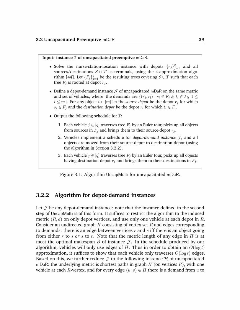
3.2 Uncapacitated Preemptive mDaR 39
Input: instance I of uncapacitated preemptive mDaR.
• Solve the nurse-station-location instance with depots rjqj=1 and allsources/destinations S ∪ T as terminals, using the 4-approximation algo-rithm [44]. Let Fjqj=1 be the resulting trees covering S ∪ T such that eachtree Fj is rooted at depot rj .
• Define a depot-demand instance J of uncapacitated mDaR on the same metricand set of vehicles, where the demands are (rj , rl) | si ∈ Fj & ti ∈ Fl, 1 ≤i ≤ m. For any object i ∈ [m] let the source depot be the depot rj for whichsi ∈ Fj and the destination depot be the depot rl for which ti ∈ Fl.
• Output the following schedule for I:
1. Each vehicle j ∈ [q] traverses tree Fj by an Euler tour, picks up all objectsfrom sources in Fj and brings them to their source-depot rj .
2. Vehicles implement a schedule for depot-demand instance J , and allobjects are moved from their source-depot to destination-depot (usingthe algorithm in Section 3.2.2).
3. Each vehicle j ∈ [q] traverses tree Fj by an Euler tour, picks up all objectshaving destination-depot rj and brings them to their destinations in Fj .
Figure 3.1: Algorithm UncapMulti for uncapacitated mDaR.
3.2.2 Algorithm for depot-demand instances
Let J be any depot-demand instance: note that the instance defined in the secondstep of UncapMulti is of this form. It suffices to restrict the algorithm to the inducedmetric (R, d) on only depot vertices, and use only one vehicle at each depot in R.Consider an undirected graph H consisting of vertex set R and edges correspondingto demands: there is an edge between vertices r and s iff there is an object goingfrom either r to s or s to r. Note that the metric length of any edge in H is atmost the optimal makespan B of instance J . In the schedule produced by ouralgorithm, vehicles will only use edges of H. Thus in order to obtain an O(log t)approximation, it suffices to show that each vehicle only traverses O(log t) edges.Based on this, we further reduce J to the following instance H of uncapacitatedmDaR: the underlying metric is shortest paths in graph H (on vertices R), with onevehicle at each R-vertex, and for every edge (u, v) ∈ H there is a demand from u to
40 Chapter 3: Multi vehicle Dial-a-Ride
v and one from v to u. Clearly any schedule for H having makespan β implies onefor J of makespan β · B. The next lemma implies an O(log |R|) approximation fordepot-demand instances.
Lemma 23. There exists a poly-time computable schedule for H with makespanO(log t), where t = |R|.
Proof: Let α = dlg te + 1. We first construct a sparse spanner A of H as follows:consider edges of H in an arbitrary order, and add an edge (u, v) ∈ H to A iff theshortest path between u and v using current edges of A is more than 2α. It is clearfrom this construction that the girth of A (length of its shortest cycle) is at least2α, and that for every edge (u, v) ∈ H, the shortest path between u and v in A is atmost 2α.
We now assign each edge of A to one of its end-points such that each vertex isassigned at most two edges. Repeatedly pick any vertex v of degree at most twoin A, assign its adjacent edges to v, and remove these edges and v from A. Weclaim that at the end of this procedure (when no vertex has degree at most 2), alledges of A would have been removed (i.e. assigned to some vertex). Suppose for acontradiction that this is not the case. Let A 6= φ be the remaining graph; note thatA ⊆ A, so girth of A is at least 2α. Every vertex in A has degree at least 3, and thereis at least one such vertex w. Consider performing a breadth-first search in A fromw. Since the girth of A is at least 2α, the first α levels of the breadth-first search isa tree. Furthermore every vertex has degree at least 3, so each vertex in the firstα − 1 levels has at least 2 children. This implies that A has at least 1 + 2α−1 > tvertices, which is a contradiction! For each vertex v ∈ R, let Av denote the edges ofA assigned to v by the above procedure; we argued that ∪v∈RAv = A, and |Av| ≤ 2for all v ∈ R.
The schedule for H involves 2α rounds as follows. In each round, every vehiclev ∈ R traverses the edges in Av (in both directions) and returns to v. Since |Av| ≤ 2for all vertices v, each round takes 4 units of time; so the makespan of this scheduleis 8α = O(log t). The route followed by each object in this schedule is the shortestpath from its source to destination in spanner A; note that the length of any suchpath is at most 2α. To see that this is indeed feasible, observe that every edge ofA is traversed by some vehicle in each round. Hence in each round, every objecttraverses one edge along its shortest path (unless it is already at its destination).Thus after 2α rounds, all objects are at their destinations.
3.2 Uncapacitated Preemptive mDaR 41
3.2.3 Tight example for uncapacitated mDaR lower bounds.
We note that known lower bounds for uncapacitated preemptive mDaR are insuffi-cient to obtain a sub-logarithmic approximation guarantee. The lower bounds weused in our algorithm are the following: maxi∈[m] d(si, ti), and the optimal value ofa nurse-station-location instance with depots rjqj=1 and terminals S ∪ T . We arenot aware of any lower bounds stronger than these two bounds.
We show an instance G of uncapacitated mDaR where the optimal makespan isa factor Ω( log t
loglog t) larger than both the above lower bounds. In fact, the instance
we construct is a depot-demand instance that has the same special structure asinstance H in Lemma 23. I.e. the demand graph is same as the graph inducingdistances. Take G = (V,E) to be a t-vertex regular graph of degree ∼ log t and girthg ∼ log t/ loglog t (there exist such graphs, eg. Lazebnik et al. [105]). Instance Gis defined on a metric on vertices V with distances being shortest paths in graphG. For every edge (u, v) ∈ E of graph G, there is an object with source u anddestination v (the direction is arbitrary). There is one vehicle located at every vertexof V ; so number of vehicles q = t.
Observe that both our lower bounds are O(1): the optimal value of the nurse-station-location instance is 0, and maximum source-destination distance is 1.However as we show below, the optimal makespan for this instance is at leastg − 1 = Ω(log t/ loglog t). Suppose (for contradiction) that there is a feasible sched-ule for G with makespan M < g − 1. A demand (u, v) ∈ E is said to be completelyserved by a vehicle j iff the route of vehicle j visits both vertices u and v. Thenumber of distinct vertices visited by any single vehicle is at most M < g: so thenumber of demands that are completely served by a single vehicle is at most M − 1(otherwise these demand edges would induce a cycle smaller than the girth g).Hence the number of demands that are completely served by some vehicle is at mostt · g < |E|. Let (u, v) ∈ E be a demand that is not completely served by any vehicle,i.e. there is no vehicle that visits both u and v. Since we have a feasible scheduleof makespan M , the path π followed by demand (u, v) from u to v (or vice versa)in the schedule has length at most M . The path π can not be the direct edge (u, v)since demand (u, v) is not completely served by any vehicle. So path π togetherwith edge (u, v) is a cycle of length at most M + 1 < g in graph G, contradictinggirth of G.
42 Chapter 3: Multi vehicle Dial-a-Ride
3.2.4 Improved guarantee for metrics excluding a fixed minor.
We now prove Theorem 20 that gives a constant approximation algorithm foruncapacitated mDaR on metrics induced by Kr-minor free graphs (for any fixed r).This improvement comes from using the existence of good ‘sparse covers’ in suchmetrics, as opposed to the spanner based construction in Lemma 23. This guaranteeis again relative to the above mentioned lower bounds.
Consider an instance of uncapacitated preemptive mDaR problem on metric (V, d)that is induced by an edge-weighted graph G = (V,E) containing no Kr-minor (forsome fixed r ≥ 1). We start with some definitions [21]. A cluster is any subset ofvertices. For any γ > 0 and vertex v ∈ V , N(v, γ) := u ∈ V | d(u, v) ≤ γ denotesthe set of vertices within distance γ from v. As observed in Busch et al. [21], thepartitioning scheme of Klein et al. [99] implies the following result.
Theorem 24 ([99]). Given Kr-minor free graph G = (V,E,w) and value γ > 0, thereis an algorithm that computes a set Z = C1, · · · , Cl of clusters satisfying:
1. The diameter of each cluster is at most O(r2) ·γ, i.e. maxu,v∈Ci d(u, v) ≤ O(r2) ·γfor all i ∈ [l].
2. For every v ∈ V , there is some cluster Ci ∈ Z such that N(v, γ) ⊆ Ci.
3. For every v ∈ V , the number of clusters in Z that contain v is at most O(2r).
The set of clusters Z found above is called a sparse cover of G.
Theorem 25. There is an O(1)-approximation algorithm for the uncapacitated pre-emptive mDaR problem on metrics induced by graphs that exclude any fixed minor.
Proof: The reduction in Section 3.2 implies that it suffices to consider depot-demand instances: An O(1) approximation for such instances implies an O(1)approximation for general instances. Let J be any depot-demand instance onmetric (V, d) induced by Kr-minor free graph G = (V,E), with a set R ⊆ V ofdepot-vertices (each containing a vehicle), and where all demands si, timi=1 arebetween vertices of R. The algorithm is described in Figure 3.2.
Note that γ is a lower bound on the optimal makespan of J . We first claim thatthe makespan of the above schedule is at most O(1) · γ. Observe that each depot iscontained in at most O(2r) clusters, and the distance from any depot to the centerof any cluster containing it is at most O(r2) ·γ. Hence the time taken by each vehicle
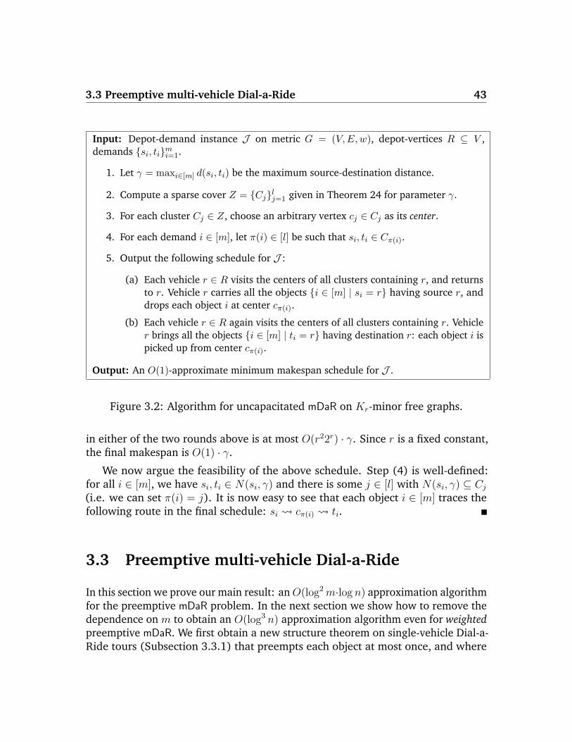
3.3 Preemptive multi-vehicle Dial-a-Ride 43
Input: Depot-demand instance J on metric G = (V,E,w), depot-vertices R ⊆ V ,demands si, timi=1.
1. Let γ = maxi∈[m] d(si, ti) be the maximum source-destination distance.
2. Compute a sparse cover Z = Cjlj=1 given in Theorem 24 for parameter γ.
3. For each cluster Cj ∈ Z, choose an arbitrary vertex cj ∈ Cj as its center.
4. For each demand i ∈ [m], let π(i) ∈ [l] be such that si, ti ∈ Cπ(i).
5. Output the following schedule for J :
(a) Each vehicle r ∈ R visits the centers of all clusters containing r, and returnsto r. Vehicle r carries all the objects i ∈ [m] | si = r having source r, anddrops each object i at center cπ(i).
(b) Each vehicle r ∈ R again visits the centers of all clusters containing r. Vehicler brings all the objects i ∈ [m] | ti = r having destination r: each object i ispicked up from center cπ(i).
Output: An O(1)-approximate minimum makespan schedule for J .
Figure 3.2: Algorithm for uncapacitated mDaR on Kr-minor free graphs.
in either of the two rounds above is at most O(r22r) · γ. Since r is a fixed constant,the final makespan is O(1) · γ.
We now argue the feasibility of the above schedule. Step (4) is well-defined:for all i ∈ [m], we have si, ti ∈ N(si, γ) and there is some j ∈ [l] with N(si, γ) ⊆ Cj(i.e. we can set π(i) = j). It is now easy to see that each object i ∈ [m] traces thefollowing route in the final schedule: si cπ(i) ti.
3.3 Preemptive multi-vehicle Dial-a-Ride
In this section we prove our main result: anO(log2m·log n) approximation algorithmfor the preemptive mDaR problem. In the next section we show how to remove thedependence on m to obtain an O(log3 n) approximation algorithm even for weightedpreemptive mDaR. We first obtain a new structure theorem on single-vehicle Dial-a-Ride tours (Subsection 3.3.1) that preempts each object at most once, and where
44 Chapter 3: Multi vehicle Dial-a-Ride
the total time spent by objects in the vehicle is bounded. Obtaining such a singlevehicle tour is crucial in our algorithm for preemptive mDaR, which appears inSection 3.3.2. The algorithm for mDaR relies on a partial coverage algorithm Partialthat given subsets Q of vehicles and D of demands, outputs a schedule for Q ofnear-optimal makespan that covers some fraction of demands in D. The main stepsin Partial are as follows. (1) Obtain a single-vehicle tour satisfying 1-preemptive andbounded-delay properties (Theorem 27), (2) Randomly partition the single vehicletour into |Q| equally spaced pieces, (3) Solve a matching problem to assign someof these pieces to vehicles of Q that satisfy a subset of demands D, (4) A suitablefraction of the unsatisfied demands in D are covered recursively by unused vehiclesof Q.
3.3.1 Capacitated Vehicle Routing with Bounded Delay
Before we present the structural result on Dial-a-Ride tours, we consider the classiccapacitated vehicle routing problem [74] with an additional constraint on object‘delays’. Recall from Chapter 2 that the capacitated vehicle routing problem (CVRP)is a special case of single vehicle Dial-a-Ride when all objects have the same source(or equivalently, same destination). Formally, we are given a metric (V, d), specifieddepot-vertex r ∈ V , and m objects all having source r and respective destinationstii∈[m]. The goal is to compute a minimum length non-preemptive tour of a capacityk vehicle originating at r that moves all objects from r to their destinations. InCVRP with bounded delay, we are additionally given a delay parameter α > 1, andthe goal is to find a minimum length capacitated non-preemptive tour serving allobjects such that the time spent by each object i ∈ [m] in the vehicle is at mostα · d(r, ti). The preemptive lower bounds (c.f. Section 2.1) in the context of CVRPare as follows [74]: minimum length TSP tour on r ∪ ti | i ∈ [m] (Steiner lowerbound), and 2
k
∑mi=1 d(r, ti) (flow lower bound).
Theorem 26. There is a (2.5 + 3α−1
) approximation algorithm for CVRP with boundeddelay, where α > 1 is the delay parameter. This guarantee is relative to the Steiner andflow lower bounds.
Proof: Our algorithm is basically a combination of the algorithms for light approxi-mate shortest path trees [97], and capacitated vehicle routing [74]. Let LB denotethe maximum of the Steiner and flow lower bounds. The minimum TSP tour onthe destinations plus r is the Steiner lower bound. The first step is to computean approximately minimum TSP tour C: Christofides’ algorithm [34] gives a 1.5
3.3 Preemptive multi-vehicle Dial-a-Ride 45
approximation, so d(C) ≤ 1.5 · LB. Number the vertices in the order in which theyappear in C, starting with r being 0. Using the procedure in Khuller et al. [97], weobtain a set of edges (0, v1), · · · , (0, vt) with 0 < v1 < v2 < · · · < vt < |V | havingthe following properties (below v0 = 0).
1. For 1 ≤ p ≤ t, for any vertex u with vp−1 ≤ u < vp, the length of edge (0, vp−1)plus the path along C from vp−1 to u is at most α · d(0, u).
2.∑t
p=1 d(0, vp) ≤ 1α−1· d(C).
For each 1 ≤ p ≤ t, define tour Cp which starts at r, goes to vp−1, traversesC until vp, then returns to r. Assign vertices vp−1, · · · , vp − 1 (and all demandscontained in them) to Cp. Also define tour Ct+1 which starts at r, goes to vt,and traverses C until r; and assign all remaining demands to Ct+1. It is clearthat Cp (for 1 ≤ p ≤ t + 1) visits each vertex assigned to it within α times theshortest path from r (using property 1 above). Also, the total length
∑t+1p=1 d(Cp) =
d(C) + 2∑t
p=1 d(0, vp) ≤ (1 + 2α−1
)d(C).
For each Cp, we service the set Dp of demands assigned to it separately. Indexthe demands inDp in the order in which they appear on Cp (breaking ties arbitrarily).Consider a capacitated tour which serves these demands in groups of at most keach, and returns to r after serving each group. The groups are defined as follows:starting at index 1, each group contains the next k contiguous demands (until all ofDp is assigned to groups). By rotating the indexing of demands, there are k differentgroupings of Dp that can be obtained: each of which corresponds to a capacitatedtour. As argued in [74] (and is easy to see), the average length of these k tours is atmost d(Cp) + 2
∑z∈Dp
d(r,z)k
. So the minimum length tour γp among these satisfies
d(γp) ≤ d(Cp) + 2∑
z∈Dpd(r,z)k
.
The final solution γ is the concatenation of tours γ1, · · · , γt+1. Note that the timespent in the vehicle by any demand i is at most α · d(r, ti). The length of tour γ isat most
∑t+1p=1 d(Cp) + 2
∑z∈D
d(r,z)k
, where D is the set of all demands. Note that2∑
z∈Dd(r,z)k
is the flow lower bound for this single-source instance, so it is at mostLB. Hence we obtain the following.
d(γ) ≤ (1 +2
α− 1)d(C) + LB ≤ (1 +
2
α− 1)3
2LB + LB = (2.5 +
3
α− 1)LB
Clearly, solution γ satisfies the desired conditions in the theorem.
46 Chapter 3: Multi vehicle Dial-a-Ride
We now consider the single vehicle preemptive Dial-a-Ride problem given bymetric (V, d), set D of demands, and a vehicle of capacity k. The following structuralresult (Theorem 27) is a simple extension of Theorem 16 (from Chapter 2). This isobtained immediately by using Theorem 26 in the proof of Theorem 16, in place ofthe [74] algorithm.
Theorem 27. There is a randomized poly-time computable 1-preemptive tour τ ser-vicing D that satisfies the following conditions (where LBpmt is the maximum of theSteiner and flow lower bounds):
1. Total length: d(τ) ≤ O(log2 n) · LBpmt.
2. Bounded delay:∑
i∈D Ti ≤ O(log n)∑
i∈D d(si, ti) where Ti is the total timespent by object i ∈ D in the vehicle under the schedule given by τ .
3.3.2 Algorithm for preemptive mDaR
We are now ready to present our algorithm for preemptive multi-vehicle Dial-a-Ride. The algorithm first guesses the optimal makespan B of the given instance ofpreemptive mDaR (it suffices to know B within a constant factor, which is requiredfor a polynomial-time algorithm). Let α = 1 − 1
1+lgm. For any subset P ⊆ [q], we
abuse notation and use P to denote both the set of vehicles P and the multi-set ofdepots corresponding to vehicles P .
We give an algorithm Partial that takes as input a tuple 〈Q,D,B〉 where Q ⊆ [q]is a subset of vehicles, D ⊆ [m] a subset of demands and B ∈ R+, with the promisethat vehicles Q (originating at their respective depots) suffice to completely servethe demands D at a makespan of B. Given such a promise, Partial 〈Q,D,B〉 re-turns a schedule of makespan O(log n logm) · B that serves a good fraction of D.Algorithm Partial〈Q,D,B〉 is given below. We set parameter ρ = Θ(log n logm), theprecise constant in the Θ-notation comes from the analysis.
Algorithm Partial〈Q,D,B〉 for capacitated preemptive mDaR.Input: Vehicles Q ⊆ [q], demands D ⊆ [m], bound B ≥ 0 such that Q can serve all demandsin D at makespan B.
Preprocessing
1. If the minimum spanning tree (MST) on vertices Q contains an edge of length greaterthan 3B, there is a non-trivial partition Q1, Q2 of Q with d(Q1, Q2) > 3B. For
3.3 Preemptive multi-vehicle Dial-a-Ride 47
j ∈ 1, 2, let Vj = v ∈ V | d(Qj , v) ≤ B and Dj be all demands of D inducedon Vj . Run in parallel the schedules from Partial〈Q1, D1, B〉 and Partial〈Q2, D2, B〉.Assume this is not the case in the following.
Random partitioning
2. Obtain single-vehicle 1-preemptive tour τ using capacity k and serving demands D,by applying Theorem 27.
3. Choose a uniformly random offset η ∈ [0, ρB] and cut edges of tour τ at distancespρB + η | p = 1, 2, · · · along the tour to obtain a set P of pieces of τ .
4. C ′′ is the set of objects i ∈ D such that i is carried by the vehicle in τ over someedge that is cut in Step (3); and C ′ := D \ C ′′. Ignore C ′′ objects in the rest of thealgorithm.
Load rebalancing
5. Construct bipartite graph H with vertex sets P and Q and an edge between pieceP ∈ P and depot f ∈ Q iff d(f, P ) ≤ 2B. For any subset A ⊆ P, Γ(A) ⊆ Q denotesthe neighborhood of A in graph H. Let S ⊆ P be any maximal set that satisfies|Γ(S)| ≤ |S|2 .
6. Compute a 2-matching π : P \ S → Q \ Γ(S), i.e. function s.t. (P, π(P )) is an edgein H for all P ∈ P \ S, and the number of pieces mapping to any f ∈ Q \ Γ(S) is|π−1(f)| ≤ 2.
Recursion
7. Define C1 := i ∈ C ′ | either si ∈ S or ti ∈ S; and C2 := C ′ \ C1.
8. Run in parallel the recursive schedule Partial〈Γ(S), C1, B〉 for C1 and the followingfor C2:
(a) Each vehicle f ∈ Q \ Γ(S) traverses the pieces π−1(f), moving all C2-objects inthem from their source to preemption-vertex, and returns to its depot.
(b) Each vehicle f ∈ Q \ Γ(S) again traverses the pieces π−1(f), this time movingall C2-objects in them from their preemption-vertex to destination, and returnsto its depot.
Output: A schedule of Q of makespan (16 + 16ρ) ·B that serves an αlg min|Q|,2m fractionof D.
48 Chapter 3: Multi vehicle Dial-a-Ride
Lemma 28. If there exists a schedule of vehicles Q covering all demands D, havingmakespan at most B, then Partial invoked on 〈Q,D,B〉 returns a schedule of vehiclesQ of makespan at most (16 + 16ρ) ·B that covers at least an αlg z fraction of D, wherez := min|Q|, 2m ≤ 2m.
The final algorithm invokes Partial iteratively until all demands are covered:each time with the entire set [q] of vehicles, all uncovered demands, and bound B.If D ⊆ [m] is the set of uncovered demands at any iteration, Lemma 28 implies thatPartial〈[q], D,B〉 returns a schedule of makespan O(logm log n) · B that serves atleast 1
4|D| demands. Hence a standard set-cover analysis implies that all demands
will be covered in O(logm) rounds, resulting in a makespan of O(log2m log n) ·B.
It remains to prove Lemma 28. We proceed by induction on the number |Q|of vehicles. The base case |Q| = 1 is easy: the tour τ in Step (2) has lengthO(log2 n) ·B ≤ ρB, and satisfies all demands (i.e. fraction 1). In the following, weprove the inductive step, when |Q| ≥ 2.
Preprocessing. Suppose Step (1) applies. Note that d(V1, V2) > B and hencethere is no demand with source in one of V1, V2 and destination in the other. Sodemands D1 and D2 partition D. Furthermore in the optimal schedule, vehicles Qj
(any j = 1, 2) only visit vertices in Vj (otherwise the makespan would be greaterthan B). Thus the two recursive calls to Partial satisfy the assumption: there is someschedule of vehicles Qj serving Dj having makespan B. Inductively, the schedulereturned by Partial for each j = 1, 2 has makespan at most (16 + 16ρ) ·B and coversat least αlg c · |Dj| demands from Dj, where c ≤ min|Q|−1, 2m ≤ z. The schedulesreturned by the two recursive calls to Partial can clearly be run in parallel and thiscovers at least αlg z(|D1|+ |D2|) demands, i.e. an αlg z fraction of D. So we have thedesired performance in this case.
Random partitioning. The harder part of the algorithm is when Step (1) doesnot apply: so the MST length on Q is at most 3|Q| ·B. Note that when the depots Qare contracted to a single vertex, the MST on the end-points of D plus the contracteddepot-vertex has length at most |Q| · B (the optimal makespan schedule inducessuch a tree). Thus the MST on the depots Q along with end-points of D has lengthat most 4|Q| ·B. Based on the assumption in Lemma 28 and the flow lower bound,we have
∑i∈D d(si, ti) ≤ k|Q| · B. It follows that for the single vehicle Dial-a-Ride
instance solved in Step (2), the Steiner and flow lower-bounds (denoted LBpmt inTheorem 27) are O(1) · |Q|B. Theorem 27 now implies that τ is a 1-preemptive tourτ servicing D, of length at most O(log2 n)|Q| ·B such that
∑i∈D Ti ≤ O(log n) · |D|B,
where Ti denotes the total time spent in the vehicle by demand i ∈ D. The bound
3.3 Preemptive multi-vehicle Dial-a-Ride 49
on the delay uses the fact that maxmi=1 d(si, ti) ≤ B.
Choosing a large enough constant corresponding to ρ = Θ(log n logm), thelength of τ is upper bounded by ρ|Q| ·B (since n ≤ 2m). So the cutting procedure inStep (3) results in at most |Q| pieces of τ , each of length at most 2ρB. The objectsi ∈ C ′′ (as defined in Step (4)) are called a cut objects. We restrict attention to theother objects C ′ = D \ C ′′ that are not ‘cut’. For each object i ∈ C ′, the path tracedby it (under single vehicle tour τ) from its source si to preemption-point and thepath (under τ) from its preemption-point to ti are both completely contained inpieces of P. Figure 3.3 gives an example of objects in C ′ and C ′′, and the cuttingprocedure.
Claim 29. The expected number of objects in C ′′ is at most∑
i∈DTiρB≤ O( 1
logm) · |D|.
Proof: The probability (over choice of η) that object i ∈ D is cut equals TiρB
where Ti is the total time spent by i in tour τ . Using linearity of expectation and∑i∈D Ti ≤ O(log n) · |D|B, we have the claim.
We can derandomize Step (3) and pick the best offset η (there are at most poly-nomially many combinatorially distinct offsets). Claim 29 implies (again choosinglarge enough constant in ρ = Θ(log n logm)) that |C ′| ≥ (1 − 1
2 lgm)|D| ≥ α · |D|
demands are not cut. Now onwards we only consider the set C ′ of uncut demands.Let P denote the pieces obtained by cutting τ as above, recall |P| ≤ |Q|. A pieceP ∈ P is said to be non-trivial if the vehicle in the 1-preemptive tour τ carries someC ′-object while traversing P . Note that the number of non-trivial pieces in P is atmost 2|C ′| ≤ 2m: each C ′-object appears in at most 2 pieces, one where it is movedfrom source to preemption-vertex and other from preemption-vertex to destination.Retain only the non-trivial pieces in P; so |P| ≤ min|Q|, 2m = z. The pieces in Pmay not be one-to-one assignable to the depots since the algorithm has not takenthe depot locations into account. We determine which pieces may be assigned todepots by considering a matching problem between P and the depots in Step (5)and (6).
Load rebalancing. The bipartite graph H (defined in Step (5)) represents whichpieces and depots may be assigned to each other. Piece P ∈ P and depot f ∈ Q areassignable iff d(f, P ) ≤ 2B, and in this case graph H contains an edge (P, f). Weclaim that corresponding to the ‘maximal contracting’ set S (defined in Step (5)),the 2-matching π (in Step (6)) is guaranteed to exist. Note that |Γ(S)| ≤ |S|
2, but
|Γ(T )| > |T |2
for all T ⊃ S. For any T ′ ⊆ P \ S, let Γ(T ′) denote the neighborhoodof T ′ in Q \ Γ(S). The maximality of S implies: for any non-empty T ′ ⊆ P \ S,
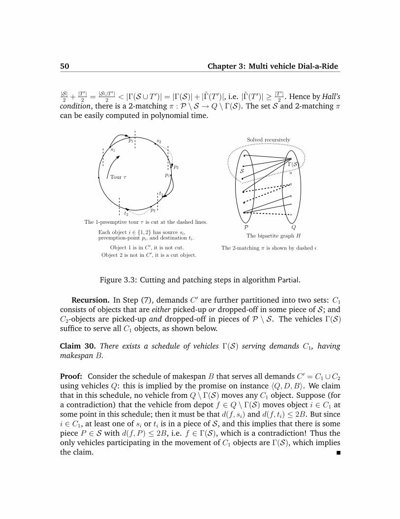
50 Chapter 3: Multi vehicle Dial-a-Ride
|S|2
+ |T ′|2
= |S∪T ′|2
< |Γ(S ∪ T ′)| = |Γ(S)|+ |Γ(T ′)|, i.e. |Γ(T ′)| ≥ |T ′|2
. Hence by Hall’scondition, there is a 2-matching π : P \ S → Q \ Γ(S). The set S and 2-matching πcan be easily computed in polynomial time.
Tour τ p1
s1
t2p2
t1
p1
p2
The 1-preemptive tour τ is cut at the dashed lines.
Object 1 is in C ′, it is not cut.
Object 2 is not in C ′, it is a cut object.
s2
SΓ(S)
P Q
The bipartite graph H
The 2-matching π is shown by dashed edges.
Solved recursively
Each object i ∈ 1, 2 has source si,preemption-point pi, and destination ti.
Figure 3.3: Cutting and patching steps in algorithm Partial.
Recursion. In Step (7), demands C ′ are further partitioned into two sets: C1
consists of objects that are either picked-up or dropped-off in some piece of S; andC2-objects are picked-up and dropped-off in pieces of P \ S. The vehicles Γ(S)suffice to serve all C1 objects, as shown below.
Claim 30. There exists a schedule of vehicles Γ(S) serving demands C1, havingmakespan B.
Proof: Consider the schedule of makespan B that serves all demands C ′ = C1 ∪C2
using vehicles Q: this is implied by the promise on instance 〈Q,D,B〉. We claimthat in this schedule, no vehicle from Q \ Γ(S) moves any C1 object. Suppose (fora contradiction) that the vehicle from depot f ∈ Q \ Γ(S) moves object i ∈ C1 atsome point in this schedule; then it must be that d(f, si) and d(f, ti) ≤ 2B. But sincei ∈ C1, at least one of si or ti is in a piece of S, and this implies that there is somepiece P ∈ S with d(f, P ) ≤ 2B, i.e. f ∈ Γ(S), which is a contradiction! Thus theonly vehicles participating in the movement of C1 objects are Γ(S), which impliesthe claim.
3.3 Preemptive multi-vehicle Dial-a-Ride 51
In the final schedule, a large fraction of C1 demands are served by vehiclesΓ(S), and all the C2 demands are served by vehicles Q \ Γ(S). Figure 3.3 shows anexample of this partition.
Serving C1 demands. Based on Claim 30, the recursive call Partial 〈Γ(S), C1, B〉(made in Step (8)) satisfies the assumption required in Lemma 28. Since |Γ(S)| ≤|P|2≤ |Q|
2< |Q|, we obtain inductively that Partial 〈Γ(S), C1, B〉 returns a schedule
of makespan (16 + 16ρ) · B covering at least αlg y · |C1| demands of C1, wherey = min|Γ(S)|, 2m. Note that y ≤ |Γ(S)| ≤ |P|/2 ≤ z/2 (as |P| ≤ z), whichimplies that at least αlg z−1|C1| demands are covered.
Serving C2 demands. These are served by vehiclesQ\Γ(S) using the 2-matchingπ, in two rounds as specified in Step (8). This suffices to serve all objects in C2
since for any i ∈ C2, the paths traversed by object i under τ , namely si pi (itspreemption-point) and pi ti are contained in pieces of P \ S. Furthermore,since |π−1(f)| ≤ 2 for all f ∈ Q \ Γ(S), the distance traveled by vehicle f in oneround is at most 2 · 2(2B + 2ρB). So the time taken by this schedule is at most2 · 4(2B + 2ρB) = (16 + 16ρ) ·B.
The schedule of vehicles Γ(S) (serving C1) and vehicles Q \ Γ(S) (serving C2)can clearly be run in parallel. This takes time (16 + 16ρ) · B and covers in totalat least |C2| + αlg z−1|C1| ≥ αlg z−1|C ′| ≥ αlg z|D| demands of D. This proves theinductive step of Lemma 28. Using Lemma 28 repeatedly as mentioned earlier,we obtain an O(log2m · log n) approximation algorithm. Using some preprocessingsteps (described in the next subsection), we have Theorem 21.
3.3.3 Weighted preemptive mDaR
The multi-vehicle Dial-a-Ride problem as initially defined assumes that all objectshave the same ‘weight’, i.e. each object occupies a unit capacity. In the weightedmDaR problem, each object i ∈ [m] also has a weight wi, and the capacity constraintrequires that no vehicle carry a total weight of more than k at any time. In thissection, we obtain an O(log3 n) approximation algorithm for weighted preemptivemDaR. The algorithm first guesses the optimal makespan B of the given instance.The algorithm serves the demands in two phases: the 1st phase involves pre-processing ‘heavy demands’ and has a makespan of O(1) · B; the 2nd phase isidentical to the algorithm Partial in Section 3.3.2 and covers all remaining demands.For every u, v ∈ V let demu,v denote the total weight of objects having source u anddestination v. Define H = (u, v) ∈ V × V | demu,v ≥ k/2 to be the vertex-pairs
52 Chapter 3: Multi vehicle Dial-a-Ride
having heavy demands, and H the set of demands between pairs of H.
Phase I. In this pre-processing step, we cover all demands H. Below we use the samenotation P ⊆ [q] for a set P of vehicles and the multi-set of depots correspondingto P . For a subset D ⊆ H of heavy vertex-pairs, let D denote the set of demandsbetween pairs of D. We describe an algorithm PreProc that serves demands H.
Lemma 31. Given any subset Q ⊆ [q] of vehicles and D ⊆ H of heavy demand-pairssuch that there is a schedule of vehicles Q covering demands D with makespan atmost B, PreProc〈Q,D〉 returns a schedule of vehicles Q covering demands D that hasmakespan O(1) ·B.
Invoking PreProc〈[q], H〉 gives the desired schedule covering H at makespanO(1) ·B. The algorithm PreProc and its analysis follow along the lines of algorithmPartial in Section 3.3.2. Lemma 31 is proved by induction on |Q|, the base case|Q| = 1 is trivial, and in the following we consider the inductive step (where|Q| ≥ 2).
Algorithm PreProc first ensures that each edge of the minimum spanning tree onQ has length at most 3B, otherwise the problem decouples into two disjoint smallerproblems (as in Step (1) of Partial). Hence we also obtain that the MST on Q plusall sources/destinations in D has length at most O(1) · |Q|B (c.f. algorithm Partial).Demands with source u and destination v are referred to as (u, v) demands. Forevery (u, v) ∈ D, using a greedy procedure, one can partition all (u, v) demandssuch that the total weight of each part (except possibly the last) is between k
2
and k. For any (u, v) ∈ D, let gu,v denote the number of parts in this partition of(u, v) demands; note that gu,v ≤ 2
kdemu,v + 1 ≤ 4
kdemu,v (since demu,v ≥ k/2). The
flow lower bound resulting from demands D equals 1|Q|k
∑(u,v)∈D demu,v · d(u, v) ≥
14|Q|∑
(u,v)∈D gu,v · d(u, v). In the rest of algorithm PreProc, we consider each part inthe above partition of (u, v) demands (for (u, v) ∈ D) as a single object of weightk; so all the objects in one part will always be moved together. Scaling downthe weights and capacity by k, we obtain the following equivalent unit-weightunit-capacity instance U : for each (u, v) ∈ D there are gu,v demands with weight 1,source u and destination v, and each vehicle in Q has capacity 1.
The flow lower bound of the demands H in the original instance implies that1
4|Q|∑
(u,v)∈H gu,v · d(u, v) ≤ B; i.e. the flow bound in U is at most 4|Q|B. SinceU has unit capacity and weights, we can use the Stacker-crane algorithm [58] toobtain a single vehicle non-preemptive tour τ serving all demands, having length 1.8times the preemptive lower bounds. The single vehicle preemptive lower bounds
3.3 Preemptive multi-vehicle Dial-a-Ride 53
corresponding to U are: (Steiner bound) TSP on all sources/destinations in D, and(flow bound)
∑(u,v)∈H gu,v · d(u, v). As shown above, these are both O(1) · |Q|B.
The algorithm next cuts tour τ to obtain at most |Q| pieces P such that each piecehas length O(1) · B. In addition it can be ensured that no demand is ‘cut’: sincethe vehicle carries at most one object at any time and each source-destinationdistance is at most B. Next, construct bipartite graph H with vertex sets P andQ and an edge between piece P ∈ P and depot f ∈ Q iff d(f, P ) ≤ 2B; Γ(A)denotes the neighborhood of any A ⊆ P in H. The algorithm finds any maximalset S ⊆ P with |Γ(S)| < |S|/2 (as in Step (5) of Partial). This implies a 2-matchingπ : P \ S → Q \ Γ(S) such that there exists a schedule of vehicles Γ(S) servingdemands in the pieces S with makespan B (c.f. Claim 30). Let C ⊆ D denotethe heavy demand-pairs served in some piece of S. The final schedule returnedby PreProc〈Q,D〉 involves: (i) schedule for vehicles Q \ Γ(S) given by π (coveringdemand-pairs D \ C); and (ii) schedule for vehicles Γ(S) obtained recursivelyPreProc〈Γ(S), C〉 (covering demands C). The recursively obtained schedule hasmakespan O(1) ·B by the induction hypothesis (since |Γ(S)| < |Q|, and 〈Γ(S), C〉satisfies the assumption in Lemma 31); hence the final schedule also has makespanO(1) ·B, which proves the inductive step.
Phase II. Let L = (u, v) ∈ V × V | 0 < demu,v < k/2 be the vertex-pairshaving light demands. The algorithm for this phase treats all (u, v) demands asa single object of weight demu,v from u to v; so there are m = |L| ≤ n2 distinctobjects. The algorithm is identical to Partial of Section 3.3.2 for the unweightedcase: Theorem 27 generalizes easily to the weighted case, and the preemptive lowerbounds stay the same after combining demands in L. Thus we obtain an O(log3 n)approximate schedule that covers all remaining demands (setting m ≤ n2).
Theorem 32. There is an O(log3 n) approximation for weighted preemptive mDaR.
Credits: This chapter is based on joint work with Inge Li Gørtz and R.Ravi.

Chapter 4
Stochastic Demands Vehicle Routing
4.1 Introduction
The capacitated vehicle routing problem (CVRP) [74] is defined on an n-vertexmetric (V, d) with root/depot r ∈ V , and involves distributing (identical) itemsfrom the depot to other vertices using a single vehicle of capacity Q ∈ N. Thereis a demand of qv ∈ 0, 1, · · · , Q at each vertex v ∈ V . The objective is to find aminimum length tour of the vehicle that satisfies all demands such that the vehiclecarries at most Q units at any time. There are two versions of the problem: in thesplit-delivery CVRP, the demand at a vertex may be satisfied by multiple visits of thevehicle; whereas in unsplit-delivery CVRP, the entire demand at a vertex must besatisfied in a single visit by the vehicle.
We consider the situation where the demands are uncertain. Here the exactdemands qvv∈V are not known in advance, instead we are only given a demanddistribution D. The actual demand at a vertex is observed only when that vertex isvisited. In this setting, a feasible solution is any strategy of visiting vertices using thecapacitated vehicle such that all realized demands are satisfied. We note that thisstrategy may be adaptive, i.e. at any point in the tour, the next vertex to visit maydepend on the demands observed until then. The stochastic vehicle routing problem(SVRP) is: given metric (V, d) with root r ∈ V , a vehicle of capacity Q ∈ N, anddemand distribution D over 0, 1, · · · , QV , compute a strategy of visiting vertices(starting and ending at r) that satisfies all realized demands, and minimizes theexpected tour length.
The most general setting of SVRP is where we are only given a black-box access
55
56 Chapter 4: Stochastic Demands Vehicle Routing
to the distribution D. However as we show in Section 4.4, no o(n) approximationratio can be achieved for the black-box model, assuming a polynomial number ofsamples from D. We consider the following two natural ways of describing thedemand distribution, that make SVRP more tractable.
• Independent demand distribution. Here, the demand at each vertex v ∈ Vis specified by a random variable ξv (in the range 0, 1, · · · , Q), and therandom variables ξvv∈V are independent of each other. This setting isextensively studied in the operations research literature [147, 16, 139], andis known as the vehicle routing problem with stochastic demands (VRPSD).
• Explicit demand distribution. Here we are givenm demand scenarios, whereeach scenario i ∈ [m] specifies demands qiv ∈ 0, 1, · · · , Q at all vertices v ∈ Vand a probability pi (where
∑mi=1 pi = 1). For each scenario i ∈ [m], let
qi ∈ 0, 1, · · · , QV denote the vector of demands qivv∈V . In the explicit-demand setting, the realized demands will always be one of q1, · · · , qm, whereqi occurs with probability pi (for all i ∈ [m]).
We refer to any tour that starts and ends at r as an r-tour.
4.1.1 Results
We first consider SVRP under independent demand distributions. We obtain arandomized approximation algorithm for VRPSD achieving the following worst-caseguarantees: (1 + α) for split-delivery VRPSD, and (2 + α) for unsplit-delivery VRPSD,where α denotes the best approximation ratio for the traveling salesman problem.This result matches (up to an additive o(1) term) the corresponding best knownguarantees for the deterministic CVRP. Furthermore, this algorithm gives an apriori strategy, that visits all vertices in a fixed order. For the split-delivery VRPSD,[16] had suggested a ‘cyclic heuristic’ and conjectured that it achieves a constantapproximation guarantee; we show that this is indeed the case by giving a 1 + 2αworst-case bound.
In Section 4.2 we consider SVRP under explicit demands, and present anO(log2 n · logm) approximation algorithm (recall, n is the number of vertices and mis the number of scenarios). Our algorithm applies to both split and unsplit deliveryversions of SVRP. We show that even a special case of SVRP under explicit demandsis at least as hard to approximate as the ‘latency group Steiner tree problem’, forwhich there is an Ω(log1−ε n) hardness of approximation [78] and O(log2 n) is the
4.1 Introduction 57
best known approximation guarantee. The main step of this algorithm lies in solvingthe related metric isolation problem that seeks to identify the realized scenario atminimum expected cost (formal definition in Section 4.3).
The adaptive strategy for the metric isolation problem proceeds in O(logm)phases, where in each phase it reduces the number of candidate scenarios by aconstant factor: so that after the last phase, it uniquely identifies the realizedscenario. In each phase of this algorithm, we solve a variant of the group Steinertree problem. We show that the LP-rounding for group Steiner tree combined withthe greedy approach for the minimum latency problem [29, 45] gives an O(log2 n)approximation algorithm for the ‘latency group Steiner tree’ problem. This leadsto an O(log2 n · logm) approximation for metric isolation. We also observe thatthe approximability of this problem is at least as hard as group Steiner tree [62],for which O(log2 n · logm) is the best known approximation ratio, and there is anΩ(log2−ε n) hardness of approximation [78].
We note that in the special case of a weighted-star metric, the metric isolationproblem corresponds to the ‘optimal split tree’ problem [101] (discussed furtherin Section 4.3.3). In this case, our approximation guarantee improves to O(logm).Hence we also obtain an O(logm)-approximation algorithm for the split tree prob-lem (where m is the number of ‘items’), answering an open question from [2].
Finally in Section 4.4, we study SVRP under black-box distributions. We showthat any algorithm that makes at most nc samples from the black-box distribution(for any c n
logn) has an approximation guarantee Ω(n
c). This is an information
theoretic lower bound and requires no assumption on the running time of thealgorithm. The basic idea is that a small number of samples from the distribution isinsufficient to learn enough about it to output a good adaptive strategy (whereas anoptimal strategy that knows the precise distribution can perform much better).
Remark. A crucial difference in the explicit-demand and independent-demandmodels is the following. As argued in Section 4.2, under independent demands,the minimum length TSP on metric (V, d) is a lower bound. However the optimalvalue of SVRP under explicit demand distributions may be much smaller than theminimum length TSP. This partly explains the difference in approximability of thesetwo versions of SVRP.
58 Chapter 4: Stochastic Demands Vehicle Routing
4.1.2 Related Work
Capacitated VRP. Let α ≥ 1 denote the best approximation guarantee for theTraveling Salesman Problem; so α = 3
2for general metrics [34], and α = 1 + ε (for
any constant ε > 0) for constant dimensional Euclidean metrics [11, 110]. The bestknown approximation guarantee for split-delivery CVRP is 1 + α · (1− 1
Q) [74, 6],
and for unsplit-delivery CVRP is 2 + α · (1 − 2Q
) [5]. These bounds have beenimproved slightly (when Q ≥ 3) to 1 + α · (1− 1
Q)− 1
3Q3 and 2 + α · (1− 2Q
)− 13Q3
respectively [19].
Independent demands VRP. SVRP under independent stochastic demands (knownas VRPSD in the literature) is extensively studied from a computational view-point [147, 42, 14, 43, 139]. In terms of worst-case bounds, a ‘cyclic heuristic’for split-delivery VRPSD was suggested in [16]. This was shown to achieve a(1 + α + o(1))-approximation in the special case of identical demand distributions;for general distributions, it was shown to be a Q+ α approximation, and obtaininga tighter bound was left open. Bertsimas [16] considered two settings for VRP withindependent demands: only the first setting (called Strategy a) applies to VRPSD asdefined in this chapter. The second setting (Strategy b) [16] is more along the linesof a priori optimization, which is discussed next.
Optimal Split Trees. When the underlying metric is a star, the metric isolationproblem turns out to be the optimal split tree problem, which was first studiedin [101]. We give a formal definition and discuss this problem in Section 4.3.3.Kosaraju et al. [101] gave a greedy algorithm for metric isolation on unweightedstar-metrics that achieves an O(logm) approximation ratio (recall, m is the numberof scenarios). Later, Adler and Heeringa [2] analyzed the same greedy algorithmfor this problem and gave an lnm+ 1 worst-case bound, and showed that this resultalso holds for weighted star-metrics but under a uniform probability distribution.Chakravarthy et al. [24] showed that the optimal split tree problem is Ω(logm)hard to approximate in general (this uses a non-uniform probability distribution);and that it is hard to approximate better than 4 when the probability distributionis uniform. This line of work leaves open the question of approximating generaloptimal split trees [2] (i.e. metric isolation on weighted star-metrics with non-uniform probabilities).
a priori Traveling Salesman. This is another stochastic model for the TSP [92, 15],which is quite different from our setting. Here we are given a metric (V, d) anddistribution D on the demands; for TSP (which is CVRP when Q =∞), a scenariois just a subset of vertices that need to be visited, and D is some distribution over

4.2 SVRP under Independent Demands 59
subsets of V . The goal is to compute an a priori (or a master) tour τ through allvertices of V , that minimizes the expectation (over scenarios in D) of the lengthof tour τ after short-cutting it to include only the vertices of the realized scenario.This corresponds to a situation where demands at all vertices are known before thevehicle starts its route (so that it can shortcut accordingly); however, we require asingle master tour to be computed beforehand. On the other hand, in SVRP (thatwe study in this chapter) the demand at any vertex is revealed only when thatvertex is visited; and we allow the vehicle-route to be adaptive. The complexity ofa priori TSP also depends on how the distribution D is represented. Schalekampand Shmoys [136] give an O(log n) approximation for this problem even underblack-box distributions; in fact their master tour does not even depend on thedistribution. Shmoys and Talwar [143] give a randomized 4-approximation (anda deterministic 8-approximation) algorithm for a priori TSP under independentdemands; a constant factor approximation for this setting can also be inferredfrom [65].
4.2 SVRP under Independent Demands
In this section, we consider SVRP under independent demand distributions. Weare given a metric (V, d) with root r ∈ V , and a demand distribution D specifiedby a random variable ξv (in the range 0, 1, · · · , Q) for each vertex v ∈ V , wherethe random variables ξvv∈V are independent of each other. The objective isto compute a strategy of visiting vertices (starting and ending at r) that servesall realized demands and minimizes the expected tour-length. This is knownas the vehicle routing problem with stochastic demands (VRPSD) in the literature,eg. [147, 16, 139]. Throughout this section, we let α denote the best approximationratio for the TSP.
Without loss of generality, we may assume that none of the demand randomvariables is identically zero (such vertices may be safely ignored). Under thisassumption, any feasible policy must visit every vertex with probability 1: otherwise,since demands are independent, there is a non-zero probability that some demand isnot satisfied (implying that the policy is infeasible). Therefore the minimum lengthTSP tour on all vertices in metric (V, d) is a lower bound for VRPSD.
This suggests the following obvious strategy of serving demands: (1) first visitall vertices using an α-approximate TSP tour and observe all demands; (2) then(since exact demands are known) serve them using the approximation algorithm
60 Chapter 4: Stochastic Demands Vehicle Routing
for CVRP [74, 5, 6]. This gives approximation ratios of (2α + 1) for split-deliverySVRP, and (2α + 2) for unsplit-delivery SVRP.
We improve over the above naıve approach in two ways. Firstly, our algorithmachieves improved approximation ratios, that match the best known for the deter-ministic versions. Secondly, our algorithm also works in the setting where demandsare observed only when they are served (see also Section 4.3.4); whereas the naıveapproach clearly depends on observing demand before serving it.
Given the demand realization qi at each vertex i ∈ V , LB(q) := 2Q
∑i∈V qi·d(r, i) is
a lower bound on the optimal solution length for split-delivery VRP (c.f. Haimovichand Kan [74]). Hence the expected value, E[LB(q)] = 2
Q
∑i∈V E[ξi] · d(r, i) is a
lower bound for VRPSD (both split/unsplit delivery versions). This lower boundand the TSP bound were also used in Bertsimas [16].
We now present our algorithms for VRPSD.
Theorem 33. There is a randomized (1 + α)-approximation algorithm for VRPSDwith split-deliveries.
Proof: The algorithm SplitALG proceeds as follows.
1. Compute an α approximate TSP tour τ on all vertices.
2. Number vertices such that r is 0 and τ visits vertices in order 0, 1, 2, · · · , |V | − 1.
3. Choose a uniformly random demand q0 ∈ [0, Q] as demand at the depot.
4. The vehicle starts at vertex 0 (filled to capacity Q), and for i = 0, 1, · · · , |V | − 1 does:
(a) Let Qi be the units (of the item) carried by the vehicle when it visits vertex i.
(b) Let qi be the demand observed at vertex i, as it is being served.
(c) If qi ≤ Qi then serve the demand at i and move on to vertex i + 1 (withQi+1 ← Qi − qi).
(d) If qi > Qi then serve Qi units of demand at i and make a visit to-and-from r:
• The vehicle fills up to Q units at r, returns to i and serves the remainingqi − Qi demand at i.
Then move on to vertex i+ 1 with Qi+1 ← Q+ Qi − qi.
We will bound the expected length of the solution obtained by the above al-gorithm. In the analysis, we first condition on the realization qi of demands at all
4.2 SVRP under Independent Demands 61
vertices i ∈ V \ r. The demand qr = q0 at the depot r remains uniformly randomin [0, Q]. A vertex i ∈ V is called a break-point if the vehicle executes a refill trip tor from i (i.e. Step 4d applies at vertex i). This happens precisely when the vehiclebecomes empty at vertex i while there is still unserved demand at i. Observe thatvertex i is a break-point iff there is p ∈ N such that
∑j<i qj ≤ p ·Q < qi +
∑j<i qj.
Since q0 (the artificial demand at r) is the only random variable, and it is is uniformin [0, Q], we have:
Pr[i is break-point] =qiQ
The solution length (conditioned on demands qii∈V \r) equals d(τ)+2∑
i 6=r d(r, i)·I(i break-point), where I(i break-point) is the indicator random variable for i beinga break-point (for each i 6= r). Hence the expected solution length (conditioned onthe demands qii∈V \r) is:
d(τ) + 2∑i 6=r
Pr[i is break-point] · d(r, i) = d(τ) +2
Q
∑i 6=r
qi · d(r, i) = d(τ) + LB(q)
Finally, the expected (unconditional) solution length equals d(τ) + E[LB(q)]. Sinceτ is an α-approximate minimum TSP tour and E[LB(q)] is a lower bound for VRPSD,the expected length of this solution is at most (1 + α) times the optimal value of theVRPSD instance. Note that algorithm SplitALG only observes demand at a vertexwhile serving it; so it gives a feasible strategy even in the SVRPobs setting.
Theorem 34. There is a randomized (2 + α)-approximation algorithm for VRPSDwith unsplit-deliveries.
Proof: The algorithm UnsplitALG is very similar to the split-delivery case and isgiven below.
1. Compute an α approximate TSP tour τ on all vertices.
2. Number vertices such that r is 0 and τ visits vertices in order 0, 1, 2, · · · , |V | − 1.
3. Choose a uniformly random demand q0 ∈ [0, Q] as demand at the depot.
4. The vehicle starts at vertex 0 (filled to capacity Q), and for i = 0, 1, · · · , |V | − 1 does:
(a) Let Ui be the units (of the item) carried by the vehicle when it visits vertex i.
(b) Let qi be the demand observed at vertex i.
(c) If qi ≤ Ui then serve demand i and move on to vertex i+1 (with Ui+1 ← Ui−qi).
62 Chapter 4: Stochastic Demands Vehicle Routing
(d) If qi > Ui then make two visits to-and-from r:
• In the first visit, the vehicle fills up to qi units at r and serves demand i.• In the second visit, the vehicle fills up to Q+ Ui − qi units at r, and returns.
Then move on to vertex i+ 1 with Ui+1 ← Q+ Ui − qi.
We first condition on the realization qi of demands at all vertices i ∈ V . Again,vertex i ∈ V is called a break-point if the vehicle executes a refill trip to r fromi (i.e. Step 4d applies at vertex i). We claim that the breakpoints encounteredby Algorithms SplitALG and UnsplitALG (for the same realization of demands) areidentical. This follows from the observation that for all vertices i ∈ V , Qi (inSplitALG) equals Ui (in UnsplitALG).
Now conditioning only on demands qii∈V \r, from the proof of Theorem 33,we have Pr[i is break-point] = qi
Qfor algorithm UnsplitALG as well. Note that the
solution length in UnsplitALG equals d(τ) + 4∑
i 6=r d(r, i) · I(i break-point), whereI(i break-point) is the indicator random variable for i being a break-point (for eachi 6= r). Hence the expected solution length (conditioned on qii∈V \r) is:
d(τ) + 4∑i 6=r
Pr[i is break-point] ·d(r, i) = d(τ) + 2 · 2
Q
∑i 6=r
qi ·d(r, i) = d(τ) + 2 ·LB(q)
Unconditionally, the expected solution length from UnsplitALG is d(τ) + 2 · E[LB(q)].Noting that τ is an α-approximate TSP tour, and E[LB(q)] is a lower bound for evensplit-delivery VRPSD, we obtain that UnsplitALG achieves a (2 + α) approximationfor unsplit-delivery VRPSD.
We now consider the cyclic heuristic for split-delivery VRPSD suggested in [16].This involves computing an α-approximate TSP tour τ , and visiting vertices in theorder given by τ while returning to the depot to fill up whenever the vehicle isempty. This is precisely algorithm SplitALG without the randomly chosen demand atthe depot (i.e. without Step 3). In fact, the algorithm suggested in [16] considers ndifferent strategies: based on rotating the vertex ordering in τ (obtained by varyingthe first vertex visited from r), and picks the one with least expected value. Weprove a constant-factor upper bound for even the (possibly weaker) algorithm thatonly considers a single vertex ordering on τ . It was shown [16] that the cyclicheuristic (using n rotations) achieves a worst case guarantee of α + 1 + o(1) in thecase of identical demand distributions at all vertices, and a Q + α guarantee forgeneral demands ([16], Theorem 4). Moreover it was conjectured that the worstcase guarantee of the cyclic heuristic is a constant (independent of Q) even with
4.2 SVRP under Independent Demands 63
general demand distributions. The following theorem shows that this is indeed thecase.
Theorem 35. The cyclic heuristic is a (1 + 2α)-approximation algorithm for split-delivery VRPSD.
Proof: Let τ visit vertices in the order 0, 1, 2, · · · , |V | − 1 with r being numbered 0.As in the proof of Theorem 33, we first condition on the demand realization qi ateach vertex i ∈ V . A vertex i ∈ V is called a break-point if the vehicle executes arefill trip to r from i. Let U be the set of all break-points (including r) and |U | = u.Then the length of the vehicle’s route is d(τ) + 2
∑w∈U d(r, w). We now establish
the following key claim.
Claim 36. We have 2 ·∑w∈U d(r, w) ≤ d(τ) + 2Q
∑v∈V qv · d(r, v).
Proof: Let the break-points U consist of r = β0, β1, · · · , βu−1 in that order alongτ . For any l ∈ 0, 1, · · · , u − 1 := [u], let τl denote the portion of tour τ betweenvertices βl and βl+1 (the indices are modulo u). Note that τ is the concatenationτ0 · τ1 · · · τu−1, i.e.
∑u−1l=0 d(τl) = d(τ). For each l ∈ [u], define a subtour originating
and ending at r as πl := (r, βl) · τl · (βl+1, r). Observe that the route τ ′ traced by thevehicle is precisely the concatenation π0 · π1 · · · πu−1. Since the vehicle capacityis Q and it makes refill-trips only when it runs out of items, the vehicle deliversexactly Q units in each segment πl (for 0 ≤ l ≤ u− 2), and Q′ ≤ Q units in the lastsegment πu−1. For each l ∈ [u] and vertex i ∈ τl, let Cl(i) denote the number ofunits delivered at vertex i by the vehicle in segment πl. For technical reasons, setCu−1(r) := Q−Q′. From the preceding discussion, we obtain:∑
i∈τl
Cl(i) = Q, ∀l ∈ [u], and∑l|i∈τl
Cl(i) = qi, ∀i ∈ V \ r (4.1)
Consider any fixed segment πl (for l ∈ [u]). For any vertex i ∈ τl, let t(i, βl) (resp.t(i, βl+1)) denote the length along τl, from βl to i (resp. i to βl+1). It follows thatt(i, βl) + t(i, βl+1) = d(τl) for all vertices i ∈ τl. By the triangle inequality, we have:
d(βl, r) ≤ d(βl, i) + d(i, r) ≤ t(βl, i) + d(i, r)d(βl+1, r) ≤ d(βl+1, i) + d(i, r) ≤ t(βl+1, i) + d(i, r)
for all vertices i ∈ τl
Taking a convex combination of the first (resp. second) set of inequalities, withmultiplier Cl(i)/Q for each i ∈ τl, we obtain the following. (Equation (4.1) implies
64 Chapter 4: Stochastic Demands Vehicle Routing
that these are indeed convex multipliers.)
d(βl, r) ≤∑i∈τl
Cl(i)
Q·(t (βl, i) + d (i, r)) ; d(βl+1, r) ≤
∑i∈τl
Cl(i)
Q·(t (βl+1, i) + d (i, r))
Adding these two inequalities (using properties of t(·) and Cl(·) from above),
d(βl, r) + d(βl+1, r) ≤∑i∈τl
Cl(i)
Q· (t (βl, i) + t (βl+1, i)) + 2
∑i∈τl
Cl(i)
Q· d (i, r)
= d(τl)∑i∈τl
Cl(i)
Q+
2
Q
∑i∈τl
Cl(i) · d(i, r)
= d(τl) +2
Q
∑i∈τl
Cl(i) · d(i, r)
Finally adding the above inequality over l ∈ [u], where the indices l are modulo u,
2 ·∑w∈U
d(w, r) =u−1∑l=0
(d(βl, r) + d(βl+1, r)) ≤u−1∑l=0
d(τl) +2
Q
∑i∈V
∑l|i∈τl
Cl(i) · d(i, r)
≤ d(τ) +2
Q
∑i∈V \r
qi · d(i, r)
The last inequality uses Equation (4.1). Thus we obtain the claim.
Claim 36 gives 2·∑w∈U d(r, w) ≤ d(τ)+LB(q), which implies that conditioned ondemands qii∈V , the solution length is at most 2 ·d(τ) + LB(q). Taking expectations,we obtain the desired bound on the cyclic heuristic.
Remarks: We note that our algorithms for VRPSD do not even require knowledgeof the demand distributions at different vertices: it suffices to know just whichvertices have a non-zero demand distribution. This information is used to computethe α-approximate TSP tour τ on relevant vertices. Furthermore, the algorithmssuggest an a priori strategy that involves visiting vertices in the order given by τ .
Theorem 33 also gives an a priori strategy for SVRP under black-box distribu-tions, having expected tour length at most α ·Tsp + OPT, where OPT is the optimalvalue of the SVRP instance and Tsp is the minimum length tour on all vertices in(V, d). This strategy does not even depend on the demand-distribution. HoweverTsp is not a lower bound for SVRP in general, hence this algorithm does not provide
4.3 SVRP under Explicit Demands 65
any multiplicative approximation guarantee. In fact, as shown in Section 4.4, anyalgorithm making at most polynomial number of samples achieves only an Ω(n)-approximation for SVRP under black-box distributions.
4.3 SVRP under Explicit Demands
In explicit demands SVRP, the distribution D is given by m scenarios, where eachscenario i ∈ [m] specifies demands qiv ∈ 0, 1, · · · , Q at all vertices v ∈ V andits associated probability pi (such that
∑mi=1 pi = 1). For each scenario i ∈ [m],
qi ∈ 0, 1, · · · , QV denotes the vector qivv∈V of demands. We assume (withoutloss of generality) that qi 6= qj for all 1 ≤ i < j ≤ m. The objective is to compute anadaptive strategy of visiting vertices starting from r (and finally returning to r) suchthat all realized demands are satisfied, and the expected tour length is minimized.For ease of exposition, we focus only on the split delivery version of SVRP; it is easyto extend our algorithm to the unsplit delivery version as well. We note that theminimum length TSP is not a lower bound for SVRP under explicit demands; hencean approach as in Section 4.2 does not suffice here.
Our algorithm for SVRP relies on the closely related metric isolation problem(Metric Isolation) which we now define. The input to the metric isolation problem isthe same as that for SVRP: metric (V, d) with root r ∈ V , and a demand distribu-tion D specified by m demand-vectors qimi=1 with associated probabilities pimi=1
(where∑m
i=1 pi = 1). However in this case, we seek a strategy of visiting vertices(starting and ending at r) that precisely determines (i.e. ‘isolates’) the realizedscenario among [m], and has the minimum expected tour length. Again this strategymay be adaptive. Note that unlike SVRP we do not require the realized demands tobe satisfied; it suffices to observe demands at vertices and stop once the realizedscenario is inferred.
Definition 37. Any feasible solution to Metric Isolation can be represented as a decisiontree T with nodes labeled by vertices of the metric, where:
1. The root node of T and all leaf-nodes are labeled r.
2. Every internal node v of T has at most Q + 1 children ci(v) | 0 ≤ i ≤ Q,where ci(v) (if present) denotes the next vertex to be visited from v if the demandobserved at v equals i.
66 Chapter 4: Stochastic Demands Vehicle Routing
3. For each scenario i ∈ [m], there is a distinct leaf node li in T such that whendecision tree T is run with realized demands qi, the path from the root node to liis traced in T .
For each i ∈ [m], let πi denote the path traced in T under scenario i, i.e. the path fromroot node to leaf li; this also corresponds to the r-tour traversed in the metric when i isthe realized scenario. The expected isolation cost of the strategy given by decision treeT is then:
IsolateTime(T ) =m∑i=1
pi · d(πi). (4.2)
The first condition implies that the route traced by the vehicle under eachscenario is an r-tour. The second condition is the definition of a decision tree.The crucial condition is the last one, which ensures that each scenario is correctlyisolated. We may assume that every node in T lies in the path traced under somescenario; otherwise the subtree under such nodes can be pruned from T . So the lastcondition also implies that the leaf nodes of T are in one-to-one correspondencewith the scenarios [m].
Lemma 38. A ρ-approximation algorithm for Metric Isolation implies a (ρ + 52)-
approximation algorithm for SVRP.
Proof: Note that by the assumption qi 6= qj for all distinct i, j ∈ [m], Metric Isolationis always feasible: the realized scenario can be correctly determined by observingdemands at all vertices. Let σ denote an optimal adaptive strategy for the givenSVRP instance, and OPT its expected length. We show below that the optimal valueof Metric Isolation is at most OPT. For each i ∈ [m], when σ is run under scenarioi, let S
idenote the demands that are observed at those vertices visited by σ. The
feasibility of σ implies that Si
contains all the non-zero demands in qi. It followsthat S
i 6= Sj
for all 1 ≤ i < j ≤ m (since qi 6= qj). Thus the demands observed whenσ is executed, identify the realized scenario uniquely. In other words σ induces afeasible solution to Metric Isolation of value OPT.
The algorithm for SVRP returns the following strategy, that runs in two phases:(1) Solve Metric Isolation (using the ρ-approximation algorithm), and execute theresulting strategy to determine the realized scenario (this phase only observesdemands); (2) Then serve only the demands in the realized scenario using the 2.5approximation algorithm for CVRP [74]. The expected cost spent in the second
4.3 SVRP under Explicit Demands 67
phase is at most 52·∑m
i=1 pi · C∗i ≤ 52· OPT, where C∗i (for each i ∈ [m]) denotes
the minimum length CVRP tour that serves demands qi. Furthermore, as observedabove, the optimal value of Metric Isolation is at most OPT. Hence the expected costin the first phase is at most ρ · OPT. This finishes the proof of the lemma.
We note that for unsplit-delivery SVRP, we could just use the correspondingalgorithm [6] in phase (2), to obtain a ρ+ 7
2approximation algorithm.
Based on this lemma, it suffices to study Metric Isolation. In the next subsection,we study two variants of the group Steiner tree problem [62] that are useful in theapproximation algorithm for Metric Isolation that we present in Section 4.3.2.
Remark. The strategy for SVRP given in Lemma 38 first explores the metric spaceand observes demands (while not serving them), and then serves just the realizedscenario. This reduction depends crucially on the fact that the demand at any vertexmay be observed by just visiting it, as opposed to actually serving its demand. Weshow in Section 4.3.4 that our algorithm can be used to obtain an O(log2 n · logm)approximate adaptive strategy even in the (more constrained) setting where anydemand is determined only upon serving it.
4.3.1 Two Auxiliary Problems
The input to the group Steiner tree problem (GST) consists of metric (V, d) withroot r ∈ V and groups Xi ⊆ V gi=1; the goal is to compute a minimum lengthr-tour covering all groups. A group i ∈ [g] is said to be covered if any vertex fromXi is visited by the tour. The best approximation guarantee known for GST isO(log2 n · log g) [62], and there is an Ω(log2−ε n) hardness of approximation [78]. Inthis section, we study two variants of group Steiner tree that are useful in obtainingan approximation algorithm for Metric Isolation.
In the latency group Steiner tree problem, in addition to the GST input we aregiven non-negative weights for each group, and the objective is to compute anr-tour covering all groups that minimizes the sum of the weighted arrival times (thearrival time of a group is the distance from r along the tour to the first vertex inthat group). This objective is closely related to Metric Isolation, which measures theexpected time to isolate a scenario, although in an adaptive (rather than linear)fashion; this observation is formalized and used in the algorithm of Section 4.3.2.
68 Chapter 4: Stochastic Demands Vehicle Routing
In the group Steiner orienteering problem, apart from the GST input there areprofits on groups and a length bound; the goal is to compute an r-tour of length atmost B that covers the maximum possible profit. It is well-known (see [18, 29, 45]on the basic latency problem) that approximations for the orienteering objectivelead to approximations for the latency objective. Following this, we start with analgorithm for the group Steiner orienteering. Then we show how this implies analgorithm for latency group Steiner, in fact for a generalization that is encounteredin Section 4.3.2.
Group Steiner Orienteering
The group Steiner orienteering (GSO) problem takes as input, a metric (V, d) withroot r ∈ V , g groups of vertices Xi ⊆ V gi=1 with associated profits vigi=1, and alength bound B. The goal is to compute an r-tour of length at most B that collectsthe maximum possible profit. We show that the deterministic algorithm for groupSteiner tree [26] can be used within a standard greedy framework to obtain thefollowing result for GSO. An algorithm for GSO is said to be an (a, b) bicriteriaapproximation if on any instance of the problem (as above), it outputs a solution oflength at most b ·B that obtains at least 1
atimes the profit obtained by any r-tour of
length B.
Theorem 39. There is a (4, O(log2 n)) bicriteria approximation algorithm for GSO,where n is the number of vertices in the metric.
Proof: Let OPT denote the optimal profit of the given GSO instance. We firstpreprocess the given metric to only include vertices within distance B/2 of the rootr (this preserves the optimal solution). Thus the profit contained in any singlevertex is at most OPT. Since the sum of profits at all vertices is at least
∑gi=1 vi, we
have 1n
∑gi=1 vi ≤ OPT. Our algorithm for GSO follows a standard greedy approach
(see eg. Garg [63]). Below we set α = O(log2 n) where the precise constant comesfrom the analysis.
1. Solution S ← ∅. Mark all groups as uncovered.
2. Until the length of S exceeds α ·B, do:
(a) Set residual profits:
vi :=
0 for each covered group i ∈ [g]vi for each uncovered group i ∈ [g]
4.3 SVRP under Explicit Demands 69
(b) Solve the following LP for the residual GSO to obtain solution (x, y):
max∑g
i=1 vi · yis.t. x(δ(S)) ≥ yi ∀S ⊆ V : r 6∈ S, Xi ⊆ S; ∀i ∈ [g]
yi ≤ 1 ∀i ∈ [g]∑e de · xe ≤ B
x, y ≥ 0
(c) As described in [26] (using probabilistic tree embedding), obtain a span-ning tree T in metric (V, d) and capacities xT on edges of T such that:∑
e∈T de · xT (e) ≤ O(log n) ·∑e de · xe ≤ O(log n) ·B, and xT supports atleast yi flow from r to Xi for each i ∈ [g].
(d) Round down each xT (e) to an integral multiple of 1n3 .
(e) For each group i ∈ [g], let y′i be the maximum flow value from r toXi under capacities xT , and let fTi (e) (for all e ∈ T ) denote the flowvariables realizing this flow.
(f) Using xT and fTi s, run the deterministic algorithm for ‘density groupSteiner’ (Section 3.2 of [26]) to obtain r-tree A covering groups A suchthat:
d(A)∑i∈A vi
≤ α · B∑gi=1 vi · y′i
, where α = O(log2 n)
(g) If d(A) ≤ αB then S ′ ← S ∪ A.
(h) If d(A) > αB then: (1) Partition tree A into at most 2 · d(A)αB
subtrees, eachof length at most αB; let A′ denote the subtree containing maximumprofit. (2) Set S ′ ← S ∪ A′ ∪ f where f is any edge from r to A′.
(i) S ← S ′. Mark all groups visited in S as covered.
3. Output an Euler tour on r-tree S.
We now prove that this algorithm achieves a (4, 4α + 2) bicriteria approximation. Itsuffices to show that the final solution S has length at most (2α+ 1) ·B and obtainsprofit at least OPT
4.
The increase in length of S in any iteration is at most (α + 1) · B (recall everyvertex is at distance at most B from r); so the final length d(S) ≤ (2α + 1) · B . Weclaim that the final solution S contains at least OPT
4profit. At any iteration, let p(S)
70 Chapter 4: Stochastic Demands Vehicle Routing
denote the profit of S, and d(S) its length. Since d(S) > αB upon termination, itsuffices to show that at all iterations in the above algorithm,
p(S) ≥ min
OPT
4,OPT
2αB· d(S)
(4.3)
We show (4.3) inductively: the base case S = ∅ is trivial. Consider any iterationwhere p(S) < OPT/4 (otherwise the claim is trivial). Hence the optimal value of theLP solved in this iteration
∑gi=1 vi · yi ≥ 3
4·OPT. After the pruning step (that rounds
down capacities) we reduce the capacity of each edge in T by at most 1n3 . Since any
cut in the tree T has at most n edges, the capacity of any cut decreases by at most1n2 after Step 2d; and by the max-flow min-cut theorem, y′i ≥ yi − 1
n2 for each i ∈ [g](in Step 2e). Furthermore, for any i ∈ [g], all the flow variables fTi correspondingto a maximum r − Xi flow are integral multiples of 1
n3 (since edge capacities xTare). This latter condition is necessary (due to technical reasons in [26]) for thealgorithm used in Step 2f. We now have:
g∑i=1
vi · y′i ≥g∑i=1
vi · yi −1
n2
g∑i=1
vi ≥3
4· OPT− 1
n2
g∑i=1
vi ≥3
4· OPT− OPT
n≥ OPT
2
where the second last inequality follows from 1n
∑gi=1 vi ≤ OPT (by the preprocess-
ing). Hence d(A)/p(A) ≤ 2α BOPT
. We finish by handling the two possible cases(Steps 2g and 2h):
• d(A) ≤ αB. Now p(S ′) = p(S) + p(A) ≥ OPT2αB· d(S) + OPT
2αB· d(A) = OPT
2αB· d(S ′).
• d(A) > αB. By averaging, we have p(A′) ≥ αB2·d(A)
p(A) ≥ OPT4
; so p(S ′) ≥ OPT4
.
In either case we have Equation (4.3) for solution S ′.
Partial Latency Group Steiner
In the partial latency group Steiner (Min-LPGST) problem, we are given a metric(V, d), g groups of vertices Xi ⊆ V gi=1 with associated weights wigi=1, root r ∈ V ,and a target h ≤ g. A group i ∈ [g] is said to be covered (or visited) by r-tour τ ifany vertex in Xi is visited, and the arrival time of such a group i is the length of theshortest prefix of τ that contains an Xi-vertex. The arrival times of all uncoveredgroups are set to be the tour-length. The weighted sum of arrival times of all groups
4.3 SVRP under Explicit Demands 71
is termed latency of the tour. The objective in Min-LPGST is to compute a minimumlatency r-tour that covers at least h groups. We present an (O(log2 n), 4) bicriteriaapproximation algorithm for Min-LPGST, i.e. the solution tour visits at least h
4groups
and has latency at most O(log2 n) times the optimal latency of a tour that visits hgroups. In the following, let Lat∗ denote the optimal value of the given instanceof Min-LPGST, and OPT∗ the length of this tour. The approximation algorithm forMin-LPGST proceeds as follows (below, we set β := 5
4, and ρ = O(log2 n) such that
the algorithm of Theorem 39 is a (4, ρ) bicriteria approximation for GSO).
1. Guess an integer l such that βl−1 < OPT∗ ≤ βl.
2. Mark all groups as uncovered.
3. For i = 1, · · · , l do:
(a) Run the GSO algorithm (Theorem 39) on the instance with groupsXigi=1, root r, length bound βi+1, and profits:
vi :=
0 for each covered group i ∈ [g]wi for each uncovered group i ∈ [g]
(b) Let τ (i) denote the r-tour obtained above. Mark all groups visited by τ (i)
as covered.
4. Construct tour τ ← τ (1) · · · τ (l), the concatenation of the r-tours found in theabove iterations. If d(τ) < ρ · βl then increase its length to ρ · βl (this may onlyincrease the latencies of groups).
5. Run the GSO algorithm on the instance with groups Xigi=1, root r, lengthbound βl, and unit profit for each group. Let σ denote the resulting r-tour.
6. Output the tour π := τ · σ as solution to the Min-LPGST instance.
Claim 40. The tour τ has length Θ(ρ) · OPT∗ and latency O(ρ) · Lat∗.
Proof: The guarantee O(ρ) · OPT∗ on the length bound is immediate from Theo-rem 39: the length of each τ (i) is at most ρ ·βi. It is also clear that d(τ) ≥ ρ ·OPT∗, bythe increase in Step 4. The proof for bounding the latency is identical to the analysisfor the Minimum Latency Problem [29, 45]. We include it here for completeness.
Fix an optimal solution ζ to the Min-LPGST instance, where d(ζ) = OPT∗ ∈(βl−1, βl]. For each i ∈ [l], let N∗i denote the total weight of groups visited in ζ by
72 Chapter 4: Stochastic Demands Vehicle Routing
time βi; note that N∗l equals the total weight of the groups covered by ζ. Similarly,for each i ∈ [l], let Ni denote the total weight of groups visited in τ (1) · · · τ (i) (i.e. byiteration i of the algorithm). Set N0 = N∗0 := 0, and W :=
∑gi=1wi the total weight
of all groups. The latency of tour τ is upper bounded by T := ρβ−1
∑li=0 β
i+2·(W−Ni).
Note also that the latency of tour ζ, Lat∗ ≥ β−1β
∑li=0 β
i(W −N∗i ).
Consider any iteration i ∈ [l] of the algorithm in Step 3. Note that the optimalvalue of the GSO instance solved in this iteration is at least N∗i − Ni−1: the βi
length prefix of tour ζ corresponds to a feasible solution to this GSO instance.Theorem 39 implies that the profit obtained in τ (i), i.e. Ni −Ni−1 ≥ 1
4· (N∗i −Ni−1),
i.e. W −Ni ≤ 34· (W −Ni−1) + 1
4· (W −N∗i ). Using this,
(β − 1)T
ρ=
l∑i=0
βi+2 · (W −Ni)
≤ 4W +1
4
l∑i=1
βi+2(W −N∗i ) +3
4
l∑i=1
βi+2(W −Ni−1)
≤ O(1) · Lat∗ +3β
4
l−1∑i=0
βi+2(W −Ni)
≤ O(1) · Lat∗ +3β
4· (β − 1)
T
ρ
Since β = 54, this implies T = O(ρ) · Lat∗, giving the claim.
Remark: The above arguments also give an O(log2 n)-approximation algorithm forthe minimum latency group Steiner problem which is Min-LPGST when h = g. Herethe objective is to minimize the sum of weighted arrival times at all groups (everygroup has to be visited). The algorithm for this problem just runs Step 3 untilall groups are covered, instead of stopping after l iterations. A proof identical tothat in Claim 40 implies an O(log2 n) approximation. Furthermore, as shown inTheorem 55, an α-approximation to latency group Steiner implies an O(α · log g)-approximation to group Steiner tree. Hence an improvement over the O(log2 n)ratio for latency group Steiner would also improve the best known bound for theusual group Steiner tree problem.
Claim 41. The tour σ covers at least h4
groups and has length O(ρ) · OPT∗.
Proof: Directly from the guarantee on GSO algorithm A (Theorem 39) invokedon the instance in Step 5: here the optimal profit is at least h, as witnessed by theoptimal solution to the Min-LPGST instance (which has length at most 2l).
4.3 SVRP under Explicit Demands 73
Theorem 42. Tour π covers at least h4
groups and has latency O(ρ) · Lat∗. Hence thereis an (O(log2 n), 4) bicriteria approximation algorithm for Min-LPGST, where n is thenumber of vertices in the metric.
Proof: Since π visits all the vertices in σ, Claim 41 implies that π covers at leasth4
groups. For each group i ∈ [g], let αi denote its arrival time under tour τ (notethat αi = d(τ) for any group i that is not covered by τ). Claim 40 implies that thelatency of tour τ ,
∑gi=1wi · αi = O(ρ) · Lat∗. Observe that for each group i that is
covered in τ , its arrival time under tour π is also αi. For any group j not covered inτ , its arrival time under π is at most d(π) (the tour length) whereas αj = d(τ). Notethat the final tour length d(π) = d(τ) + d(σ) = Θ(ρ) ·OPT∗ and d(τ) ≥ ρ ·OPT∗ (byStep 4). Hence, the arrival time under π of each group i ∈ [g] is O(1) · αi. UsingClaim 40, we obtain the theorem.
4.3.2 Algorithm for the Metric Isolation Problem
Recall that an instance of Metric Isolation is specified by metric (V, d), root r ∈ V ,and m scenarios qimi=1 with respective probabilities pimi=1. We give a recursivealgorithm for solving Metric Isolation. Given an input instance as above, we will dealwith sub-instances given by some subset M ⊆ [m] of scenarios with probabilitiessii∈M where
∑i∈M si = 1; we refer to such an instance as 〈M, sii∈M〉. Below
we describe a recursive algorithm IsoAlg that represents an adaptive strategy ofisolating the realized scenario amongst M . In the following, [Q] := 0, 1, · · · , Q.
The algorithm IsoAlg proceeds in several phases. In each phase, it maintainsa candidate set M of scenarios such that the realized scenario lies in M . Uponobserving demands along the tour produced by algorithm Partition (in Step 2), anew set M ′ ⊆M containing the realized scenario is identified such that the numberof candidate scenarios reduces by a constant factor (i.e. |M ′| ≤ 3
4· |M |); then IsoAlg
recurses on scenarios M ′. After O(logm) such phases the realized scenario wouldbe correctly identified.
Algorithm IsoAlg〈M, sii∈M〉:
1. If |M | = 1, return this unique scenario as realized.
2. Apply algorithm Partition〈M, sii∈M〉 to obtain r-tour τ given by〈r = v0, v1, v2, · · · , vl, vl+1 = r〉 and an associated partition Pktk=1 of M .
74 Chapter 4: Stochastic Demands Vehicle Routing
3. For each k ∈ [t], let s′k :=∑
i∈Pk si.
4. Traverse tour τ and return directly to r after the first vertex that reveals therealized scenario to be in some part Pk (for k ∈ [t]).
5. Run IsoAlg〈Pk, sis′k i∈Pk〉 to determine the realized scenario.
The next algorithm Partition seeks to find an r-tour τ such that after observing de-mands on τ , the candidate number of scenarios is reduced by a constant factor. Notethat each vertex v corresponds to a partition Pv = Fv,yQy=0 of M depending on theobserved demand at v (defined formally in Step 1 below). If the largest part in Pv(hence any other part) was at most a constant fraction of M , then visiting vertex vsuffices to always reduce the number of candidate scenarios by this constant factor.However the largest part in Pv may be almost all of M , in which case the tour has tovisit more vertices before substantially reducing the number of candidate scenarios.This is the basic idea behind the group Steiner instance constructed in this algorithm.
Algorithm Partition〈M, sii∈M〉:
1. For each v ∈ V and y ∈ [Q], define Fv,y := i ∈M | qiv = y, and
y(v)← arg max|Fv,y| : 0 ≤ y ≤ Q; Dv ←M \ Fv,y(v)
2. For each i ∈M , set Xi ← v ∈ V | i ∈ Dv.
3. Run the algorithm (Section 4.3.1) for the Min-LPGST instance on metric (V, d)with root r, groups Xii∈M with weights sii∈M , and target |M | − 1. Letτ := 〈r = v0, v1, v2, · · · , vl, vl+1 = r〉 be the r-tour obtained.
4. Obtain partition Pktk=1 of M as follows (Figure 4.1 gives an example):
(a) Initialize k ← 0, N ←M .
(b) For j = 1, · · · , l do:
• Define Rjx := N∩Fvj ,x for all x ∈ [Q]\y(vj), partitioning N∩D(vj).
• Let Rj(1), · · · , R
j(e) be non-empty parts in Rj
x | x ∈ [Q] \ y(vj).• For each f = 1, · · · , e, set Pk+f ← Rj
(f) and ν(k + f)← j.
• Set k ← k + e, and N ← N \D(vj).
(c) If N 6= ∅ then, set Pk+1 ← N , ν(k + 1)← l + 1 and k ← k + 1.
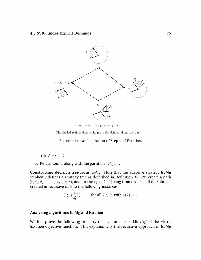
4.3 SVRP under Explicit Demands 75
r = v0 = v4
v1
v2
v3
P2 P3
P4
P5
P6
P1
The shaded regions denote the parts Pks defined along the tour τ .
Tour τ is 〈r = v0, v1, v2, v3, v4 = r〉.
Figure 4.1: An illustration of Step 4 of Partition.
(d) Set t← k.
5. Return tour τ along with the partition Pktk=1.
Constructing decision tree from IsoAlg. Note that the adaptive strategy IsoAlgimplicitly defines a strategy tree as described in Definition 37. We create a path(r, v1, v2, · · · , vl, vl+1 = r), and for each j ∈ [l+1] hang from node vj, all the subtreescreated in recursive calls to the following instances:
〈Pk, sis′k〉, for all k ∈ [t] with ν(k) = j.
Analyzing algorithms IsoAlg and Partition
We first prove the following property that captures ‘subadditivity’ of the MetricIsolation objective function. This explains why the recursive approach in IsoAlg
76 Chapter 4: Stochastic Demands Vehicle Routing
works.
Claim 43. For any partition Pktk=1 of M and s′k =∑
i∈Pk si (for k ∈ [t]), we have∑tk=1 s
′k · OPT(〈Pk, sis′k i∈Pk〉) ≤ OPT(〈M, sii∈M〉).
Proof: Let T denote the decision tree representing the optimal strategy for theMetric Isolation instance I0 := 〈M, sii∈M〉. Recall the definition of leaf-node li andpath πi (for each scenario i ∈M) from the beginning of Section 4.3. For each k ∈ [t],let Ik := 〈Pk, sis′k i∈Pk〉. Consider a feasible decision tree for Ik given by T inducedon the leaf-nodes li | i ∈ Pk (note that it is indeed feasible since T isolates allscenarios ∪tk=1Pk). Observe that the expected cost of this strategy is
∑i∈Pk
sis′k· d(πi);
hence OPT(Ik) ≤∑
i∈Pksis′k· d(πi). Summing over all parts k ∈ [t],
t∑k=1
s′k · OPT(Ik) ≤t∑
k=1
s′k ·∑i∈Pk
sis′k· d(πi) =
∑i∈M
si · d(πi) = OPT(I0)
The second last equality uses the fact that Pktk=1 is a partition of M .
We now prove that the algorithm is well-defined and establish its performanceguarantee. For any instance J of Metric Isolation, let OPT(J ) denote its optimalvalue. Let the original Metric Isolation instance be I = 〈[m], pii∈[m]〉.Claim 44. The optimal value of the Min-LPGST instance in Step 3 of algorithmPartition〈M, sii∈M〉 is at most OPT(〈M, sii∈M〉).
Proof: Let I0 = 〈M, sii∈M〉 denote the given Metric Isolation instance, and Tan optimal decision tree corresponding to it. Note that by definition of the setsDvv∈V , any internal node in T labeled vertex v has one child (namely cy(v)) thatcorresponds to the realized scenario being in Fv,y(v) = M \Dv. Consider a path σtraced from the root of T that always moves from node v to the child correspondingto M \Dv, until it reaches a leaf-node; let nodes in σ be labeled r, u1, u2, · · · , ul, r(this defines an r-tour in the metric). Since T is a feasible decision tree for theMetric Isolation instance, there is a unique scenario a ∈M such that when T is rununder demands qa, it traces the root-leaf path σ. In other words, every scenariob ∈M \ a gives rise to a root-leaf path (the path πb in Definition 37) that divergesfrom σ. However from the construction of σ, it follows that the scenarios divergingfrom it are precisely ∪lj=1Duj = M \ a.
Now consider the r-tour r, u1, u2, · · · , uj, r in metric (V, d) (corresponding toσ) as a solution to the Min-LPGST instance. The number of groups covered is
4.3 SVRP under Explicit Demands 77
| ∪lj=1 Duj | = |M | − 1, so it is indeed feasible. Furthermore, it is easy to see fromthe definition of the isolation cost (4.2) that the latency of this solution is at mostIsolateTime(T ), i.e. at most OPT(I0).
Consider the tour τ := 〈r = v0, v1, · · · , vl, r = vl+1〉 obtained in Step 3 ofPartition. For every i ∈ M , let αi denote the arrival time for group i in tour τ (seeSection 4.3.1 for the definition). Also let Lat(τ) :=
∑i∈M si · αi denote the latency
of tour τ . Theorem 42 and Claim 44 imply that τ covers | ∪lj=1 Dvj | ≥ |M |4
groups,and:
Lat(τ) ≤ ρ · OPT(〈M, sii∈M〉), where ρ := O(log2 n) (4.4)
We now show some properties of the partition Pktk=1 constructed in Step 4.
Claim 45. After Step 4 of Partition, we have |Pk| ≤ 34|M | for each k ∈ [t].
Proof: We first show that |Pk| ≤ 12|M | for every part Pk produced in the itera-
tions of Step 4b. This is immediate from the observation that for all vertices vand x ∈ [Q] \ y(v), |Fv,x| ≤ |M |
2(since Fv,y(v) is the largest sized part among
Fv,0, Fv,1, · · · , Fv,Q).
There may be at most one part that is produced after Step 4b, i.e. the last Pt inStep 4c. From the construction, it follows that this part is precisely M \ ∪lj=1D(vj).In other words, these are all the uncovered groups in the solution τ for the Min-LPGST instance. Theorem 42 implies that τ covers at least 1
4(|M |− 1) groups; hence
|M \ ∪lj=1D(vj)| ≤ 34|M |. So this extra part has size at most 3
4|M |.
Claim 46. After Step 4 of Partition, for all k ∈ [t] and i ∈ Pk, the arrival time of groupi in tour τ is αi =
∑ν(k)j=1 d(vj−1, vj).
Proof: This is immediate from the construction of partition Pktk=1. For all partsPk (with k ∈ [t]) that are produced in Step 4b of Partition, it is clear that ν(k)equalsthe index of the first vertex in τ that contains groups of Pk. Hence the claim followsfor all groups in these parts.
For the (possibly absent) single part with ν-value l + 1 produced in Step 4c ofPartition, the groups in this part are not covered by τ . So their arrival time equalsthe tour length
∑l+1j=1 d(vj−1, vj), again as required.
Claim 47. At the end of Step 4 of IsoAlg〈M, sii∈M〉 the realized scenario lies in Pk.The expected length traversed in this step is at most 2 ·Lat(τ) ≤ 2ρ ·OPT(〈M, sii∈M〉).
78 Chapter 4: Stochastic Demands Vehicle Routing
Proof: Visiting any vertex v reveals which part among Fv,x | x ∈ [Q] the realizedscenario lies in. Now consider the construction of partition Pktk=1 in Step 4 ofPartition. Note that for any j ∈ [l], Pk | ν(k) = j are all the parts added in the j-thiteration of Step 4b; also let Pk | ν(k) = l + 1 (possibly empty) denote the singleextra part added in Step 4c. Clearly tl+1
j=1Pk | ν(k) = j = Pktk=1.
This implies that when vertex vj (any j ∈ [l+1]) is visited along τ , it is determinedwhich part (if any) among Pk | ν(k) = j the realized scenario lies in. Thus thetraversal of τ in Step 4 of IsoAlg returns to r from vertex vj (for j ∈ [l + 1]) iff therealized scenario lies in one of Pk | ν(k) = j. Hence Pk correctly contains therealized scenario after Step 4 of IsoAlg〈M, sii∈M〉.
From the above arguments, it follows that for any j ∈ [l + 1], the probability ofreturning to r from vertex vj (in Step 4 of IsoAlg) is precisely
∑k∈[t]:ν(k)=j
∑i∈Pk si.
So the expected length traversed is:
≤ 2 ·l+1∑j=1
( j∑h=1
d(vh−1, vh)
)·
∑k∈[t]:ν(k)=j
∑i∈Pk
si
(4.5)
= 2 ·t∑
k=1
ν(k)∑h=1
d(vh−1, vh)
·∑i∈Pk
si
(4.6)
= 2 ·t∑
k=1
∑i∈Pk
αi · si (4.7)
= 2 ·∑i∈M
αi · si (4.8)
Inequality (4.5) follows since the tour-length when returning from vj is at
most 2(∑j
h=1 d(vh−1, vh))
. Equality (4.6) is just an interchange of summation,
equality (4.7) is from Claim 46, and equality (4.8) uses the fact that Pktk=1
partitions M . The last expression is Lat(τ), and from Equation (4.4), we have theclaim.
Lemma 48. The expected length of the strategy given by IsoAlg〈M, sii∈M〉 is at most2ρ · (log4/3 |M |) · OPT(〈M, sii∈M〉).
Proof: We prove this by induction on |M |. The base case of |M | = 1 is trivial:zero length is traversed in this case. In the following assume |M | ≥ 2. Let I0 :=
4.3 SVRP under Explicit Demands 79
〈M, sii∈M〉, and for each k ∈ [t], let Ik := 〈Pk, sis′k i∈Pk〉. From Claim 47, theexpected length spent in Step 4 of IsoAlg(I0) is at most 2ρ ·OPT(I0). For any k ∈ [t],since |Pk| ≤ 3
4|M | (by Claim 45), the inductive hypothesis implies that the expected
length of IsoAlg(Ik) is at most:
2ρ · log4/3 |Pk| · OPT(Ik) ≤ 2ρ(log4/3 |M | − 1) · OPT(Ik).
The probability of recursing on Ik is exactly s′k for each k ∈ [t]. So the expectedlength of IsoAlg(I0) is at most:
2ρ · OPT(I0) +t∑
k=1
s′k · 2ρ · (log4/3 |M | − 1) · OPT(Ik)
≤ 2ρ · OPT(I0) + 2ρ · (log4/3 |M | − 1) · OPT(I0)
= 2ρ · log4/3 |M | · OPT(I0)
where the inequality uses Claim 43.
Thus for any Metric Isolation instance given by metric (V, d), root r, and sce-narios qi, pimi=1 (as above), the strategy IsoAlg〈[m], pii∈M〉 is O(log2 n · logm)-approximately optimal. This clearly runs in time polynomial in n and m. Asmentioned earlier, it is also easy to modify the description of algorithm IsoAlgso as to output a decision-tree representation of the resulting strategy (again inpolynomial time). Hence we obtain:
Theorem 49. There is anO(log2 n·logm) approximation algorithm for Metric Isolation,where n is number of vertices and m is number of scenarios.
4.3.3 Optimal Split Tree Problem
In the optimal split tree problem [101], we are given a set of m items with associatednon-negative weights pimi=1 (that sum to 1) and a collection Tjnj=1 of n binarytests with non-negative costs cjnj=1. Each test Tj ⊆ [m] (for j ∈ [n]) is a subsetof the items that correspond to passing the test; so performing test j distinguishesbetween items Tj and [m] \ Tj.
Definition 50. A split tree S is a binary tree where each internal node is labeled by atest, and each leaf node is labeled by an item such that:
80 Chapter 4: Stochastic Demands Vehicle Routing
• For each item i ∈ [m] define a path πi in S from the root node to some leaf asfollows. At any internal node, if i passes the test then πi follows the right branch;if it fails the test then πi follows the left branch.
• For each i ∈ [m], the path πi ends at a leaf labeled item i.
The cost Li of an item i ∈ [m] is the sum of test-costs along path πi; and the cost of thesplit tree S is
∑mi=1 pi · Li.
The objective in the optimal split tree problem is to compute a split tree ofminimum cost. As mentioned earlier, O(logm)-approximation algorithms areknown for the optimal split tree problem in the following special cases: equalitem-weights [101] or equal test-costs [2]. We show here that our algorithm forMetric Isolation implies an O(logm) approximation for the optimal split tree problem(under arbitrary item-weights and test-costs). As mentioned earlier, there is anΩ(logm) hardness of approximation for this problem [24].
We first observe that the optimal split tree problem is a special case of MetricIsolation. Given an instance of optimal split tree (as above), consider a metric (V, d)induced by a weighted star with center r and n leaves corresponding to the tests.For each j ∈ [n], we set d(r, j) =
cj2
. The demand scenarios are as follows: foreach i ∈ [m], scenario i consists of a unit demand at each of j ∈ [n] | i ∈ Tj andzero demand at all other vertices. It is easy to see that this Metric Isolation instancecorresponds exactly to the optimal split tree instance.
We now show an O(logm)-approximation algorithm for Metric Isolation instanceson weighted star metrics, which implies the same bound for the optimal split treeproblem. This improvement comes from the following strengthening of Theorem 39.
Corollary 51. There is a (1− 1e)-approximation algorithm for group Steiner orienteer-
ing on weighted star metrics.
Proof: We assume (without loss of generality) that the root r is the star-center.Consider an instance of group Steiner orienteering on a weighted star-metric (V, d)with center r and leaves [n], g groups Xi ⊆ [n]gi=1 with profits vigi=1, andlength bound B. For each j ∈ [n], define set Sj := i ∈ [g] | j ∈ Xi of costcj := d(r,j)
2. The group Steiner orienteering instance is equivalent to computing
a collection K ⊆ [n] of the sets with∑
j∈K cj ≤ B/2 that maximizes f(K) :=∑vi | i ∈ ∪j∈KSj. Observe that the latter problem is an instance of maximizing amonotone submodular function (namely f : 2[n] → R) over a knapsack constraint(i.e.
∑j∈K cj ≤ B/2), for which a 1− 1
eapproximation algorithm is known [149].
4.3 SVRP under Explicit Demands 81
Based on the framework in Section 4.3.2, the above constant approximation forGSO implies the following.
Theorem 52. There is an O(logm)-approximation algorithm for the optimal split treeproblem, where m is the number of items.
4.3.4 Issue of Observing Demands
In the stochastic vehicle routing problem as defined, the exact demand at a vertexis observed when the vehicle visits that vertex. In this section, we consider a variantwhere the demand at a vertex is not determined by merely visiting it, but only whenit is actually served. This setting only applies to the split-delivery version. We referto this variant of SVRP as SVRPobs. It is clear that for any instance of the problem,the optimal value under SVRP is at most that under SVRPobs (since the latter ismore constrained). The algorithm for SVRP does not directly extend to SVRPobs
since Lemma 38 does not hold here (see remark after Lemma 38). However thefollowing theorem shows that a suitable modification still permits a reduction fromSVRPobs to Metric Isolation.
Theorem 53. A ρ-approximation algorithm for Metric Isolation implies a (2ρ + 72)-
approximation for SVRPobs. Hence there is an O(log2 n · logm)-approximation algo-rithm for SVRPobs.
Proof: Consider any instance I of SVRPobs given by metric (V, d) with root r ∈ V ,and m scenarios given by demand-vectors qimi=1 and probabilities pimi=1. Let OPTdenote the optimal value of I considered as an SVRP instance; as noted above, theoptimal value of I under SVRPobs is at least OPT. As argued in Lemma 38, theoptimal value of the Metric Isolation instance corresponding to I is at most OPT.The algorithm for SVRPobs is:
1. Obtain a ρ-approximately optimal strategy σ for the Metric Isolation instanceof I (given by the algorithm in the assumption).
2. Return the following strategy for SVRPobs(I):
(a) Visit vertices (using the capacity Q vehicle) according to strategy σ whileservicing each vertex as it is visited (so the demands are determinedeven in the SVRPobs setting); whenever the vehicle runs out of items, itperforms a refill trip to-and-from r.
82 Chapter 4: Stochastic Demands Vehicle Routing
(b) Let k denote the realized scenario, that is identified at the end of σ.
(c) Service all remaining demands in qk using the 52-approximate tour for
CVRP [74].
For the analysis, we condition on a fixed scenario j ∈ [m] (as in the proofs for SVRPwith independent demands). Let τj denote the r-tour followed by σ under scenarioj when demands are only observed (not serviced). Note that when the strategyfor SVRPobs(I) executes step 2a, the resulting r-tour τ ′j is τj along with refill-tripsfrom some vertices on τj (where the vehicle runs out of items). We refer to anyvertex on τj from which a refill-trip is made as a breakpoint. Let Uj denote the setof all breakpoints on τj; we always include the root r in Uj. Then the length ofτ ′j is exactly d(τj) + 2
∑w∈Uj d(r, w). Using Claim 36 (Section 4.2) on tour τj, the
demands served in it, and breakpoints Uj, we obtain:
2 ·∑w∈Uj
d(r, w) ≤ d(τj) +2
Q
∑v∈V
qjv · d(r, v), ∀j ∈ [m] (4.9)
We now obtain that d(τ ′j) ≤ 2 · d(τj) + 2Q
∑v∈V q
jv · d(r, v) for each j ∈ [m]. In
other words, the expected length of Step 2a is:m∑j=1
pj · d(τ ′j) ≤ 2m∑j=1
pj · d(τj) +m∑j=1
pj ·(
2
Q
∑v∈V
qjv · d(r, v)
)≤ (2ρ+ 1) · OPT
where the last inequality uses the observations: (1)∑m
j=1 pj·d(τj) equals IsolateTime(σ),
which is at most ρ · OPT; and (2)∑m
j=1 pj ·(
2Q
∑v∈V q
jv · d(r, v)
)is a lower bound
on SVRP(I).
Finally as argued in Lemma 38, since we know the realized scenario in Step 2c,the expected length here is at most 5
2· OPT. Thus we have the theorem.
4.3.5 Hardness of Approximation
In this subsection, we provide lower bounds on the approximability of the metricisolation problem, and SVRP under explicit demands. We first observe that MetricIsolation is at least as hard to approximate as group Steiner tree. This is almostidentical to the reduction [35] from Set-cover to the optimal split tree problem;we give a proof for completeness. Combined with the result in [78], the followingtheorem implies that Metric Isolation is Ω(log2−ε n) hard to approximate.
4.3 SVRP under Explicit Demands 83
Theorem 54. An α-approximation algorithm for Metric Isolation implies an α+ o(1)approximation algorithm for group Steiner tree.
Proof: Consider an arbitrary instance of group Steiner tree on metric (V, d) withroot r and groups X1, · · · , Xg ⊆ V ; let OPT denote its optimal value. Assumewithout loss of generality that Xi 6= Xj for all i 6= j. We construct an instance ofMetric Isolation as follows. Let V ′ = V ∪ s where s is a new vertex, and definemetric d′ on V ′:
d′(u, v) :=
d(u, v) for u, v ∈ Vd(u, r) + L for u ∈ V, v = s
, ∀(u, v) ∈(V ′
2
)Above L αn ·maxu,v d(u, v) is some large value. There are g + 1 scenarios in theMetric Isolation instance: X1, · · · , Xg and Xg+1 := s, with probabilities
pi :=
1gL
if 1 ≤ i ≤ g
1− 1L
if i = g + 1,
The root in the Metric Isolation instance remains r. Let OPT′ denote the optimalisolation time of this instance. We will show that (1−o(1)) ·OPT ≤ OPT′ ≤ OPT+1which would prove the proposition.
(A) (1− o(1)) · OPT ≤ OPT′. Consider the optimal strategy for the Metric Isolationinstance; let σ denote the r-tour traversed by this strategy under scenario Xg+1.We now argue that σ is a feasible solution to group Steiner tree. Observe that theoptimal isolation time is at most n ·maxu,v d(u, v) 1
α· L: visiting all vertices in V
along any r-tour is a feasible strategy. Since pg+1 = 1− o(1), the r-tour σ does notvisit vertex s (otherwise the objective value would be at least L − 1). Hence σ isan r-tour in metric (V, d) as well. Furthermore σ must visit at least one vertex fromeach Xigi=1: otherwise scenario Xg+1 is not isolated. Thus σ is a feasible solutionto the group Steiner instance. Finally, OPT′ ≥ (1− 1
L) · d(σ) ≥ (1− 1
L) · OPT.
(B) OPT′ ≤ OPT + 1. Let τ denote an optimal r-tour for the given GST instance, sod(τ) = OPT. Consider the following strategy for Metric Isolation:
1. Traverse r-tour τ to determine whether or not Xg+1 is the realized scenario.
2. If Xg+1 is realized, stop.
3. If Xg+1 is not realized, visit all vertices in V along an arbitrary r-tour todetermine the realized scenario.
84 Chapter 4: Stochastic Demands Vehicle Routing
For any i ∈ [g + 1], let πi denote the r-tour traversed under scenario Xi in the abovestrategy. It is clear that d(πg+1) ≤ d(τ) ≤ OPT, and for all i ∈ [g], d(πi) ≤ L
α. Thus
the resulting isolation time is at most:
(1− 1
L) · OPT + g · 1
gL· Lα≤ OPT + 1
Thus we have the desired reduction.
In the latency group Steiner problem (LGST), we are given metric (V, d) withroot r, groups Xi ⊆ V gi=1 of vertices, and the goal is to compute an r-tourcovering all groups that minimizes the average arrival time at a group. As observedin Subsection 4.3.1, this is a special case of partial latency group Steiner. We nowobtain the following hardness result for SVRP under explicit demands. Combinedwith the result in [78], this implies that SVRP is Ω(log1−ε n) hard to approximate.
Theorem 55. An α-approximation algorithm for SVRP under explicit demands impliesan O(α)-approximation algorithm for LGST, which in turn implies an O(α · log g)-approximation algorithm for GST.
Proof: We first give the reduction from LGST to SVRP with explicit demands, andthen the reduction from group Steiner tree to LGST.
(I) Reducing LGST to SVRP. Consider an arbitrary instance I0 of LGST with metric(V, d), root r, and groups Xi ⊆ V gi=1; let OPT0 denote its optimal value. Bystandard scaling arguments we can assume that every edge in the metric has lengthin the range [1, n3]. For each i ∈ [g], let Tspi denote the length of the minimum TSPtour on vertices Xi, and L := maxgi=1 Tspi. Also set t := dn ·Le; it is clear that t ≤ n5.We construct a new metric (U, l) as follows: take t disjoint copies of metric (V, d)and contract all copies of vertex r to a new root s. So we have:
l(u, v) :=
d(u, v) for u, v in the same copy of Vd(u, r) + d(v, r) for u, v in distinct copies of V
For this reduction, it suffices to consider the stochastic TSP problem (which isSVRP with capacity Q =∞); hence each scenario is just a subset of vertices. In factwe consider a further special case, where upon visiting any vertex v, it is not onlyknown whether or not there is demand at v, but if there is demand at v it is alsoknown what the realized scenario is. (Eg. this can be ensured by making copies of
4.3 SVRP under Explicit Demands 85
every vertex v (at zero distance from each other) where each copy of v correspondsto exactly one of the scenarios that occur at v.)
We now define the stochastic TSP instance I on metric (U, l) with root s. Thereare m := t · g scenarios (each with equal probability), for each j ∈ [t] and i ∈ [g],the Xi-vertices in the j-th copy of (V, d) constitute a scenario. This completes thedescription of the stochastic TSP instance I, which is essentially t copies of I0. LetOPT denote the optimal stochastic TSP objective value of I, and OPTI the optimalMetric Isolation objective value of I. Note that by construction, the minimum TSPlength for each scenario is at most L; so by Lemma 38, OPTI ≤ OPT ≤ OPTI + L.Note also that OPTI ≥ Ω(t) L. Hence we have,
OPTI ≤ OPT ≤ (1 + o(1)) · OPTI (4.10)
This is main purpose of considering the scaled up instance I. The above relationbetween the SVRP and Metric Isolation objectives does not hold in arbitrary instancessuch as I0. We now establish a sequence of claims that imply OPT = Θ(t) · OPT0,which suffices to prove the theorem.
Claim 56. The optimal LGST value corresponding to I is (1 + o(1)) · OPTI .
Proof: Observe that for instance I, the Metric Isolation objective is precisely Min-LPGST where weights are 1
meach and target h = m−1. Furthermore since I consists
of t copies of the original instance I0, the optimal LGST value corresponding to I(i.e. Min-LPGST with target m) is (1 + o(1)) times the Metric Isolation value.
Claim 57. The optimal LGST value corresponding to I is O(t) · OPT0.
Proof: Fix an optimal solution ζ to I0; and for each integer i ≥ 1, let Ni denote thefraction of groups having arrival times between 2i−1 and 2i. So OPT0 ≥
∑i≥1Ni·2i−1.
We construct a feasible solution to I as follows. For each integer i ≥ 1 do: for everycopy of (V, d) in (U, l), starting from s traverse the 2i-length prefix of ζ and returnto s. It is easy to see that the latency of the resulting solution to LGST on I is atmost
∑i≥1Ni · (t · 2i+1) = O(t) · OPT0.
Claim 58. The optimal LGST value corresponding to I is Ω(t) · OPT0.
Proof: Fix an optimal solution τ to LGST on I; note that I has a total weight ofone distributed uniformly over all t copies I0. For each integer i ≥ 0, let Li be the
86 Chapter 4: Stochastic Demands Vehicle Routing
length of the shortest prefix of τ that contains weight 1− 12i
and let τi denote thisprefix. The latency of τ is:
Lat(τ) ≥∑i≥1
(Li − Li−1) · 1
2i=∑i≥1
Li ·(
1
2i− 1
2i+1
)=
1
2
∑i≥1
Li ·1
2i
We first claim that for every integer i ≥ 1, there is an r-tour σi in metric (V, d)of length at most 2
t· Li that covers at least 1− 1
2i−1 fraction of I0-groups. For eachj ∈ [t], let fj ∈ [0, 1] denote the fraction of groups in the j-th copy of I0 that arenot covered by τi. By the definition of τi, we have 1
t
∑tj=1 fj ≤ 1
2i. Thus (by Markov
inequality) there is a subset S ⊆ [t] of |S| ≥ t2
copies with fj ≤ 22i
for all j ∈ S. Nowthere is some k ∈ S such that the portion of τi in the k-th copy of I0 has length atmost Li
|S| ≤ 2 · Lit
. Thus the portion of τi in this k-th copy corresponds to an r-tourσi in metric (V, d) of length d(σi) ≤ 4 · Li
tthat covers at least 1 − 1
2i−1 fraction ofI0-groups.
Consider the solution to I0 which is the concatenation σ1 · σ2 · · · . The latency ofthis solution is at most:
d(σ1) +∑i≥2
d(σi) ·1
2i−2≤ 4 · L1
t+
16
t·∑i≥2
Li ·1
2i≤ 32
t· Lat(τ)
Thus we have the claim.
Combining Claims 56, 57 and 58 we obtain OPTI = Θ(t) · OPT0. Togetherwith Equation (4.10), this implies OPT = Θ(t) · OPT0, proving the first part of thetheorem.
(II) Reducing GST to LGST. This is a simple set-covering based reduction. Recallthat any instance I of the group Steiner tree problem consists of metric (V, d) withroot r ∈ V and groups Xi ⊆ V gi=1. The goal is to compute a minimum lengthr-tour covering all groups. Let A be any ρ-approximation algorithm for LGST; wenow describe how this may be used to obtain an O(ρ · log g)-approximation for GST.
1. Set current r-tour S ← ∅, uncovered groups U ← [g].
2. While (U 6= ∅) do:
(a) Run algorithm A on the LGST instance with metric (V, d), root r andgroups Xii∈U . Let τ be the r-tour obtained, and Lat the average arrivaltime of groups in U .
4.4 SVRP under Black-box Distribution 87
(b) Let τ ′ be the truncated tour obtained by returning to root r after traversinglength 2 · Lat along τ .
(c) Augment S ← S · τ ′.(d) Remove from U all groups covered in τ ′.
3. Output S as solution to GST.
Let OPTdenote the optimal value of the given instance I. It is clear that upontermination, the final solution S is a feasible GST solution. It only remains to boundthe length of S.
Claim 59. The solution S obtained above has length d(S) ≤ O(ρ · log g) · OPT.
Proof: Consider an arbitrary iteration where U ⊆ [g] denotes the set of uncoveredgroups. Observe that the optimal value of LGST instance restricted to U is at mostOPT: the arrival time of every group in an optimal GST solution to I is at mostOPT. Thus the average arrival time in τ is Lat ≤ ρ · OPT. So the increase in thelength of S in any iteration is at most 4ρ ·OPT. Also, by Markov inequality, at least|U |/2 groups have arrival time at most 2 · Lat in tour τ ; i.e. τ ′ covers at least |U |/2groups from U . Hence the number of uncovered groups (i.e. |U |) decreases by afactor of two in each iteration; this implies that the number of iterations is at mostdlog2 ge+ 1. The claim now follows.
Thus we have an O(ρ · log g)-approximation algorithm for GST assuming aρ-approximation for LGST. This proves the second part of the theorem.
4.4 SVRP under Black-box Distribution
In this section, we study the most general model for SVRP where the demanddistribution D is given by means of a black-box (or an oracle) from which analgorithm can draw samples. In this setting, every sample from this black-box isan independent draw from the actual demand distribution D. We provide a stronginformation-theoretic lower bound on the approximability of SVRP under black-boxdistributions. In fact this lower bound holds even in the special case of stochasticTSP where the capacity is ∞, so each scenario is just a subset of vertices to visit.We show that any algorithm that samples from the distribution D at most nc times(for any c = o(n/ log n)) achieves only an Ω(n/c) approximation ratio; recall that
88 Chapter 4: Stochastic Demands Vehicle Routing
n denotes the number of vertices in the underlying metric. In particular, thereis no o(n)-approximation algorithm for the black-box model of SVRP, that makespolynomially many samples.
Let A be any algorithm for SVRP under black-box distributions that samplesfrom the distribution at most N := nc times (for some c = o( n
logn)). We make no
assumption on the running time of A. Given any instance of SVRP, A outputs a de-cision tree corresponding to an adaptive strategy of visiting vertices (Definition 37);note that the size of this decision tree may be exponentially large, since we makeno assumption on the running time of A. We will show that there exist instances forwhich the solution produced by A has cost Ω(n
c) times the optimal.
Consider a weighted-star metric (V, d) with center r and 2t leaves A := aiti=1
and B := biti=1. The edges (r, ai) (for all i ∈ [t]) have length zero, and edges (r, bi)(for all i ∈ [t]) have length one. The number of vertices in the metric is n = 2t+ 1.Fix a parameter k := 2c, and let C :=
([t]k
)be the collection of all k-subsets of [t]. For
any M ∈ C, we define A(M) = aj | j ∈ M and similarly B(M) = bl | l ∈ M.Let F denote the set of all functions f : C → C. For every function f ∈ F , definedemand-distribution Df as containing the following scenarios uniformly at random(each scenario in Df is just a subset of vertices to be visited, specified by a k-subsetof [t]):
Df ≡ A(S) ∪B(f(S)), for all S ∈ C
For each function f ∈ F , define instance If of SVRP on metric (V, d) with demanddistribution Df , and infinite vehicle capacity. We will consider the outcome ofalgorithm A on these SVRP instances, and show that it performs poorly on at leastone of them.
Claim 60. The optimal value of each instance If is at most 2k.
Proof: This strategy first visits all vertices in A (at zero length) to observe demandsat A(S) for some S ∈ C, and then visits precisely the vertices in B(f(S)). Theresulting tour always has length 2k (since |f(S)| = k).
Note that this strategy relies crucially on the fact that it knows the exact functionf . On the other hand, when algorithm A is run on some instance If , the onlyinformation about function f that it obtains is through a set of N
(tk
)random
samples from the black-box Df . In the following we show that this informationis insufficient to compute a good solution. Below, u.a.r. stands for uniformly atrandom.
4.4 SVRP under Black-box Distribution 89
By the definition of functions f that we consider, each sample from the black-box is of the form A(A′) ∪ B(B′) where A′, B′ ∈ C. Note that for a given set ofsamples from the black-box distribution, algorithm A outputs a unique decisiontree. Conditioned on a set Q = Ai ∪BiNi=1 of samples from the black-box, let T (Q)denote the decision-tree output by A. For any set Q = Ai ∪ BiNi=1 of demand-samples, any function f ∈ F that agrees with Q (i.e. f(Ai) = Bi for all 1 ≤ i ≤ N),and any scenario S ∈ C, let L(f, S,Q) denote the number of B-vertices visitedunder decision-tree T (Q) when the realized demand is A(S) ∪B(f(S)).
Claim 61. For any set Q = Ai ∪ BiNi=1 of demand-samples and S ∈ C \ AiNi=1,Ef [L(f, S,Q)] = Ω(t) where the expectation is taken over u.a.r. function f ∈ F thatagrees with Q.
Proof: Note that conditioned on Q, algorithm A outputs the unique decision-treeT (Q). We claim that for any S ′ ∈ C, when T (Q) is run with demands A(S) ∪B(S ′),it visits all the vertices B(S ′). This follows since for any S ′ ∈ C there is somefunction f ∈ F that agrees with Q and has f(S) = S ′; and T (Q) must be a feasiblesolution to this instance If . Hence T (Q) visits all vertices in A(S) ∪ B(S ′) underthis scenario in Df . Let L(S ′, S,Q) be the number of B-vertices visited when T (Q)is run with demands A(S) ∪B(S ′). Observe that for every f ∈ F that agrees withQ and has f(S) = S ′, we have L(f, S,Q) = L(S ′, S,Q). When f ∈ F u.a.r. overfunctions that agree with Q, it is clear that Ef [L(f, S,Q)] = ES′ [L(S ′, S,Q)] (whereS ′ ∈ C u.a.r.).
We assume (without loss of generality) that decision-tree T (Q) first visits allvertices in A, since this has zero length. We focus on the decision tree T (Q,S)defined as T (Q) conditioned on observing demands at A(S); note that T (Q,S) visitsonly B-vertices. As observed above, for any S ′ ∈ C, when T (Q,S) is run withdemands B(S ′) it must visit all the vertices B(S ′), and L(S ′, S,Q) is the number ofB-vertices it visits. Let M(S ′, S,Q) ≤ L(S ′, S,Q) denote the number of B-verticesvisited by T (Q,S) under demands B(S ′) until the point it visits all of B(S ′). Wenow show a lower bound ES′ [M(S ′, S,Q)] ≥ Ω(t) that proves the claim.
Consider running decision tree T (Q,S) under u.a.r. S ′ ∈ C representing de-mands onB-vertices. Let us condition on traversing some pathO in T (Q,S) from theroot that visits at most t
2B-vertices, such that some vertex v is the next to be visited
(after O). The outcomes along path O do not include vertex v, which is the first unex-plored vertex to be visited after O. We have PrS′ [v ∈ S ′ | S ′ consistent with O] ≤ 2k
t,
since irrespective of the exact outcomes along O there are at least t2
unexploredB-vertices and at most k are in S ′. In the traversal of T (Q,S) under u.a.r. S ′ ∈ C,
90 Chapter 4: Stochastic Demands Vehicle Routing
whenever a vertex v ∈ S ′ is visited, we term it success. Note that ES′ [M(S ′, S,Q)]is precisely the expected number of vertex-visits until k successes. Consider atruncated process P that traverses T (Q,S) under u.a.r. S ′ ∈ C, and stops at theearlier of k successes or t
2vertex-visits. The expected number of vertices visited in
P is clearly at most ES′ [M(S ′, S,Q)]. Note that at any point in P, the conditionalprobability of success is at most 2k
t(from above). Now define random process P ′
that performs independent tosses of a coin with heads probability 2kt
: P ′ keepstossing the coin until either the number of tosses exceeds t
2or at least k heads
are observed. Clearly, the expected number of vertices visited in P is at least theexpected number of tosses in P ′. Finally, it is easy to see that the expected numberof tosses in P ′ is Ω(t).
The next claim is straightforward from the definitions.
Claim 62. For any function f ∈ F , the expected cost of the decision-tree producedby algorithm A is EA1,··· ,ANES[L(f, S, Ai, f(Ai)Ni=1)] where the expectation is takenover A1, · · · , AN , S ∈ C chosen independently and u.a.r.
Theorem 63. For any algorithm A that makes at most N = nc samples from theblack-box distribution (where c = o(n/ log n)), there is a function f ∈ F such thatalgorithm A achieves only an Ω(n
c) approximation on SVRP instance If .
Proof: For a fixed demand-sample Q = Ai, BiNi=1, let F(Q) := f ∈ F | f(Ai) =Bi, ∀i ∈ [N ] denote all functions in F that agree with Q. Consider the followingtwo ways of generating random tuples of the form 〈f,Q = Ai, BiNi=1〉, wheref ∈ F and A1, · · · , AN , B1, · · · , BN ∈ C.
D1 Pick A1, · · · , AN , B1, · · · , BN ∈ C u.a.r. independently to set Q = Ai, BiNi=1;then pick f ∈ F(Q) independently u.a.r.
D2 Pick u.a.r. f ∈ F ; then pick A1, · · · , AN ∈ C independently u.a.r., and setBi = f(Ai) for all i ∈ [N ] (again Q = Ai, BiNi=1).
It is easy to see that the distributions of tuples 〈f,Q〉 resulting from these twoprocedures is identical (since F includes all functions mapping C to C).
For any fixed Q = Ai, BiNi=1, taking expectation over S ∈ C chosen u.a.r.and independently in Claim 61 implies that ESEf∈F(Q)[L(f, S,Q)] = Ω(t), sincePrS[S 6∈ A1, · · · , AN] ≥ 1 − N
|C| ≥ 12. Since S and f are independent, we have
4.4 SVRP under Black-box Distribution 91
Ef∈F(Q)ES[L(f, S,Q)] = ESEf∈F(Q)[L(f, S,Q)] = Ω(t). Now taking an outer expec-tation over Q = Ai, BiNi=1,
EA1,··· ,AN ,B1,··· ,BNEf∈F(Q)ES[L(f, S,Q)] = Ω(t)
Taking an outer expectation over f ∈ F u.a.r. in Claim 62, the average solutioncost produced by A on instances If is:
EfEA1,··· ,ANES[L(f, S, Ai, f(Ai)Ni=1)] = EQEf∈F(Q)ES[L(f, S,Q)] = Ω(t)
where the first equality uses the equivalence of the two distributions (D1) and (D2)mentioned above. Since the average solution cost on instances corresponding to Fis Ω(t), there is some f ∈ F with solution cost Ω(t) = Ω(n).
Furthermore, Claim 60 implies that the optimal value of every If is at most2k = 4c. Thus we obtain the theorem.
Credits: The results in this chapter are based on joint work with Anupam Gupta,Ravishankar Krishnaswamy and R. Ravi.

Chapter 5
VRPs on Asymmetric Metrics
5.1 Introduction
In this chapter, we consider some vehicle routing problems on asymmetric metrics.An asymmetric metric is given by tuple (V, d) where V denotes the vertex-set andd : V × V → R+ is a distance function that satisfies the triangle inequality, i.e.d(u, v) + d(v, w) ≥ d(u,w) for all u, v, w ∈ V . We emphasize that the distances neednot satisfy symmetry, as in the metrics considered in previous chapters; hence forany u, v ∈ V , d(u, v) 6= d(v, u) in general.
The most basic VRP in this setting is the Asymmetric Traveling Salesman Problem(ATSP). The best known approximation ratio for ATSP is O(log n) [60] (as opposedto 3
2[34] in the symmetric version). Improving this bound is an important open
question in approximation algorithms. The problems considered in this chapterare variants of ATSP that are also directed counterparts of well-studied VRPs onsymmetric metrics. Network design problems on directed graphs are often muchharder to approximate than their undirected counterparts– the traveling salesmanand Steiner tree problems are well known examples. The currently best knownapproximation ratio for the directed Steiner tree problem is O(nε) [27] for any fixedε > 0, whereas there is a 1.55-approximation algorithm on symmetric metrics [132].
93
94 Chapter 5: VRPs on Asymmetric Metrics
5.1.1 Problem Definition and Preliminaries
We now define the directed VRPs considered in this chapter. All these problems aredefined over an asymmetric metric (V, d) with |V | = n vertices and a specified rootr ∈ V . Any tour (resp. path) starting at r is called an r-tour (resp. r-path).
Directed k-TSP. Given a target k ≤ n, the goal is to compute a minimum lengthr-tour that contains at least k other vertices. This is a generalization of the ATSP,which is obtained by setting k = n.
Minimum Ratio ATSP. This involves finding an r-tour that minimizes the ratio ofthe length of the tour to the number of vertices in it (not including the root r).Observe that if the requirement that the tour contain the root is dropped, this ratioproblem becomes the minimum mean weight cycle problem, which is exactly solvablein polynomial time [94]. However, the rooted version which we are interested in isNP-complete.
Directed Orienteering. Here we are given a length bound D, and the goal is tofind an r-path of length at most D, that visits the maximum number of vertices.The orienteering problem can also be extended to the setting where there is somenon-negative profit at each vertex, and the goal is to maximize total profit.
Directed Minimum Latency. For a directed path (or tour) π and vertices u, v ∈ V ,let dπ(u, v) denote the distance from u to v along π; if v is not reachable fromu along π, then dπ(u, v) = ∞. The directed minimum latency problem involvescomputing a spanning r-path π that minimizes
∑v∈V d
π(r, v); the quantity dπ(r, v)is the latency of vertex v in path π. Another possible definition of this problemrequires an r-tour covering all vertices, where the latency of the root r is set to bethe distance required to return to r (i.e. the total tour length); note that in theprevious definition, the latency of r is zero. As we show later in this chapter, theapproximability of both these versions of directed latency are within a constantfactor of each other. We work with the path version of directed latency.
Bicriteria approximations. Consider any problem P having the form:
minC(z) : z ∈ S, N(z) ≥ kwhere S is the feasible region, C : S → R+ is the cost function, N : S → R+ is a
5.1 Introduction 95
coverage function, and k is the target. Eg., in the directed k-TSP problem, S is theset of all r-tours; for any z ∈ S, C(z) is the length of tour z, and N(z) is the numberof vertices covered in tour z. An algorithm A for problem P is said to be an (α, β)bi-criteria approximation, if on each problem instance A obtains a solution y ∈ S sat-isfying C(y) ≤ α · OPT and N(y) ≥ k
β, where OPT = minC(z) : z ∈ S, N(z) ≥ k
is the optimal value of this instance.
For a directed multigraph G = (V,E) and any S ⊆ V , we denote by δ+(S) =(u, v) ∈ E | u ∈ S, v 6∈ S the edges leaving vertex-set S, and δ−(S) = (u, v) ∈E | u 6∈ S, v ∈ S the edges entering S. When dealing with asymmetric metrics withvertex set V , the edge set E is assumed to be V × V , unless mentioned otherwise.For any vector x : E → R+ and F ⊆ E, denote x(F ) :=
∑e∈F xe.
Multigraph G = (V,E) is called Eulerian if in-degree equals out-degree at eachvertex, i.e. |δ+(v)| = |δ−(v)| for each v ∈ V . Given G = (V,E) and verticesu, v ∈ V , the directed connectivity from u to v equals the maximum number ofedge-disjoint paths from u to v (or equivalently, the minimum number of edgeswhose removal disconnects v from u). Given a directed multigraph G = (V,E) andedges (u, v), (v, w) ∈ E, the operation of replacing edges (u, v) and (v, w) by a newedge (u,w) (i.e. E ← (E \ (u, v), (v, w)) ∪ (u,w)) is called splitting-off. Someproofs in this chapter make use of the following ‘splitting-off’ theorems for digraphs.
Theorem 64 (Mader [109]). Let G = (U ∪ v, E) be a directed multigraph suchthat the indegree equals outdegree at v, and the directed connectivity between anypair of vertices in U is at least k. Then for every edge (v, w) ∈ E there exists an edge(u, v) ∈ E so that after splitting-off edges (u, v) and (v, w), the directed connectivitybetween every pair of vertices in U remains at least k.
Theorem 65 (Frank [57] (Theorem 4.3) and Jackson [91]). Let G = (U ∪ v, E)be an Eulerian directed multigraph. For each edge (v, w) ∈ E there exists an edge(u, v) ∈ E so that after splitting-off edges (u, v) and (v, w), the directed connectivitybetween every pair of vertices in U remains the same.
Remark: Consider any vector x : E → R+ of rational edge-capacities that is Eule-rian, namely x(δ−(v)) = x(δ+(v)) at all vertices v ∈ V . Let M ∈ N be large enoughthat M · xe ∈ N for all e ∈ E. Then M · x corresponds to an Eulerian multi-graph,for which the above splitting-off theorems apply. Based on this correspondence, weuse splitting-off theorems directly on rational edge-capacities that are Eulerian.
96 Chapter 5: VRPs on Asymmetric Metrics
5.1.2 Results
We present a polynomial time O(log2 n · log k)-approximation algorithm for thedirected k-TSP problem. This is based on an O(log2 n)-approximation algorithmfor minimum ratio ATSP. To the best of our knowledge, this ratio problem has notbeen studied earlier. The main ingredient in the algorithm is a splitting-off theoremon directed Eulerian graphs. This algorithm appears in Section 5.2. We thenuse the approximation algorithm for minimum ratio ATSP, to obtain an O(log2 n)approximation guarantee for directed orienteering (Section 5.3). This answersin the affirmative, the question of poly-logarithmic approximability of directedorienteering [17].
For the directed latency problem, we present an LP-based reduction to the Asym-metric Traveling Salesman Path problem (ATSP-path) [103, 32]. We give an nO(1/ε)
time algorithm for the directed latency problem that achieves an approximationratio of O(ρ · nε
ε3) (for any 1
logn< ε < 1), where ρ is the integrality gap of an LP
relaxation for the ATSP-path problem (details in Section 5.4). We obtain an upperbound ρ = O(
√n) in Section 5.5; however we conjecture that ρ = O(log n). In par-
ticular, our result implies a polynomial time O(n1/2+ε)-approximation algorithm fordirected latency (with any fixed ε > 0), which is the first non-trivial approximationguarantee for this problem.
5.1.3 Related Work
The best known approximation guarantee for ATSP is O(log n); the first approxima-tion ratio [60] was dlog2 ne, and since then several papers improved the constantterm, leading to the currently best 2
3· log2 n bound [53].
All problems considered in this chapter are well-studied in the undirected setting.Blum et al. [17] obtained the first constant factor approximation algorithm for theorienteering problem (on symmetric metrics). This was improved to a factor of3 in Bansal et al. [13], and later to 2 + ε (for any fixed ε > 0) in Chekuri etal. [30]. Bansal et al. [13] also used orienteering as a subroutine to also obtainpoly-logarithmic approximation algorithms for some generalizations of orienteering:deadline TSP and vehicle routing problem with time windows. The first constant-factorapproximation algorithm for undirected minimum latency was given by Blum etal. [18]; following a line of improvements, the currently best known approximationratio is 3.59 due to Chaudhuri et al. [29].
5.2 Directed k-TSP 97
Chekuri and Pal [31] obtained a general approximation algorithm for a classof VRPs on asymmetric metrics, that runs in quasi-polynomial time. In particular,their result implies a quasi-polynomial time O(log n)-approximation algorithm forthe directed orienteering problem. Their result also holds for the generalizationwhen the profit is any monotone submodular set function on the vertices.
The directed latency problem turns out to be closely related to AsymmetricTraveling Salesman Path (ATSP-path) [103]. ATSP-path is a generalization of ATSP,where the goal is to compute the minimum length spanning path between specifiedend-points. Lam and Newmann [103] were the first to consider this problem, andthey gave an O(
√n) approximation based on the Frieze et al. [60] algorithm for
ATSP. This was improved to an O(log n) ratio in Chekuri and Pal [32], that extendedthe Kleinberg and Williamson [100] algorithm for ATSP. Subsequently Feige andSingh [53] showed that the approximability of ATSP and ATSP-path are within aconstant factor of each other.
5.2 Directed k-TSP
In this section, we consider the directed k-TSP problem and obtain an O(log2 n ·log k)-approximation algorithm for this problem. We first obtain an O(log2 n)-approximation algorithm for the related minimum ratio ATSP (Theorem 69), andthen show how this implies the result for directed k-TSP (Theorem 70). Ouralgorithm for minimum ratio ATSP is based on upper bounding the integrality gapof a suitable LP relaxation for ATSP (Theorem 66), which we study next.
5.2.1 A linear relaxation for ATSP
Consider the following LP relaxation for ATSP on metric (V, d).
min∑
e de · zes.t.
z(δ+(v)) = z(δ−(v)) ∀v ∈ V(ALP ) z(δ+(S)) ≥ 1 ∀∅ 6= S 6= V
ze ≥ 0 ∀ edges e
This relaxation was also studied in Vempala and Yannakakis [154], where theauthors proved a structural property about basic solutions to (ALP ). We are not
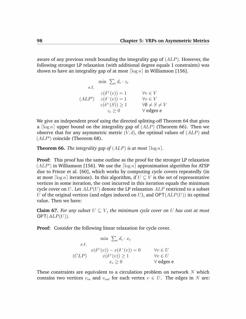
98 Chapter 5: VRPs on Asymmetric Metrics
aware of any previous result bounding the integrality gap of (ALP ). However, thefollowing stronger LP relaxation (with additional degree equals 1 constraints) wasshown to have an integrality gap of at most dlog ne in Williamson [156].
min∑
e de · zes.t.
z(δ+(v)) = 1 ∀v ∈ V(ALP ′) z(δ−(v)) = 1 ∀v ∈ V
z(δ+(S)) ≥ 1 ∀∅ 6= S 6= Vze ≥ 0 ∀ edges e
We give an independent proof using the directed splitting-off Theorem 64 that givesa dlog ne upper bound on the integrality gap of (ALP ) (Theorem 66). Then weobserve that for any asymmetric metric (V, d), the optimal values of (ALP ) and(ALP ′) coincide (Theorem 68).
Theorem 66. The integrality gap of (ALP ) is at most dlog ne.
Proof: This proof has the same outline as the proof for the stronger LP relaxation(ALP ′) in Williamson [156]. We use the dlog ne approximation algorithm for ATSPdue to Frieze et al. [60], which works by computing cycle covers repeatedly (inat most dlog ne iterations). In this algorithm, if U ⊆ V is the set of representativevertices in some iteration, the cost incurred in this iteration equals the minimumcycle cover on U . Let ALP (U) denote the LP relaxation ALP restricted to a subsetU of the original vertices (and edges induced on U), and OPT(ALP (U)) its optimalvalue. Then we have:
Claim 67. For any subset U ⊆ V , the minimum cycle cover on U has cost at mostOPT(ALP (U)).
Proof: Consider the following linear relaxation for cycle cover.
min∑
e de · xes.t.
x(δ+(v))− x(δ−(v)) = 0 ∀v ∈ U(CLP ) x(δ+(v)) ≥ 1 ∀v ∈ U
xe ≥ 0 ∀ edges e
These constraints are equivalent to a circulation problem on network N whichcontains two vertices vin and vout for each vertex v ∈ U . The edges in N are:
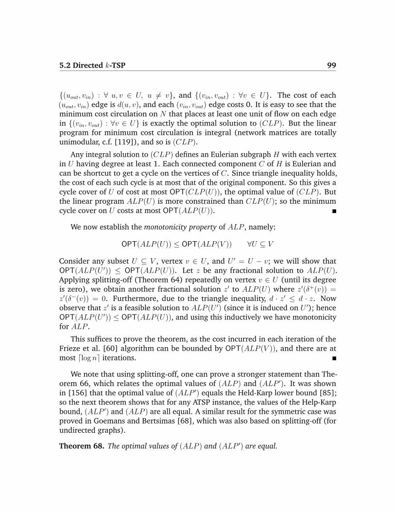
5.2 Directed k-TSP 99
(uout, vin) : ∀ u, v ∈ U, u 6= v, and (vin, vout) : ∀v ∈ U. The cost of each(uout, vin) edge is d(u, v), and each (vin, vout) edge costs 0. It is easy to see that theminimum cost circulation on N that places at least one unit of flow on each edgein (vin, vout) : ∀v ∈ U is exactly the optimal solution to (CLP ). But the linearprogram for minimum cost circulation is integral (network matrices are totallyunimodular, c.f. [119]), and so is (CLP ).
Any integral solution to (CLP ) defines an Eulerian subgraph H with each vertexin U having degree at least 1. Each connected component C of H is Eulerian andcan be shortcut to get a cycle on the vertices of C. Since triangle inequality holds,the cost of each such cycle is at most that of the original component. So this gives acycle cover of U of cost at most OPT(CLP (U)), the optimal value of (CLP ). Butthe linear program ALP (U) is more constrained than CLP (U); so the minimumcycle cover on U costs at most OPT(ALP (U)).
We now establish the monotonicity property of ALP , namely:
OPT(ALP (U)) ≤ OPT(ALP (V )) ∀U ⊆ V
Consider any subset U ⊆ V , vertex v ∈ U , and U ′ = U − v; we will show thatOPT(ALP (U ′)) ≤ OPT(ALP (U)). Let z be any fractional solution to ALP (U).Applying splitting-off (Theorem 64) repeatedly on vertex v ∈ U (until its degreeis zero), we obtain another fractional solution z′ to ALP (U) where z′(δ+(v)) =z′(δ−(v)) = 0. Furthermore, due to the triangle inequality, d · z′ ≤ d · z. Nowobserve that z′ is a feasible solution to ALP (U ′) (since it is induced on U ′); henceOPT(ALP (U ′)) ≤ OPT(ALP (U)), and using this inductively we have monotonicityfor ALP .
This suffices to prove the theorem, as the cost incurred in each iteration of theFrieze et al. [60] algorithm can be bounded by OPT(ALP (V )), and there are atmost dlog ne iterations.
We note that using splitting-off, one can prove a stronger statement than The-orem 66, which relates the optimal values of (ALP ) and (ALP ′). It was shownin [156] that the optimal value of (ALP ′) equals the Held-Karp lower bound [85];so the next theorem shows that for any ATSP instance, the values of the Help-Karpbound, (ALP ′) and (ALP ) are all equal. A similar result for the symmetric case wasproved in Goemans and Bertsimas [68], which was also based on splitting-off (forundirected graphs).
Theorem 68. The optimal values of (ALP ) and (ALP ′) are equal.
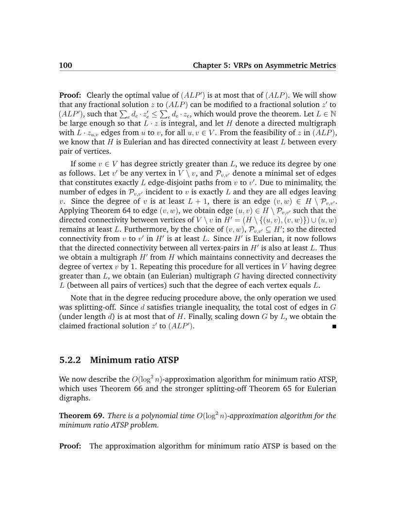
100 Chapter 5: VRPs on Asymmetric Metrics
Proof: Clearly the optimal value of (ALP ′) is at most that of (ALP ). We will showthat any fractional solution z to (ALP ) can be modified to a fractional solution z′ to(ALP ′), such that
∑e de · z′e ≤
∑e de · ze, which would prove the theorem. Let L ∈ N
be large enough so that L · z is integral, and let H denote a directed multigraphwith L · zu,v edges from u to v, for all u, v ∈ V . From the feasibility of z in (ALP ),we know that H is Eulerian and has directed connectivity at least L between everypair of vertices.
If some v ∈ V has degree strictly greater than L, we reduce its degree by oneas follows. Let v′ be any vertex in V \ v, and Pv,v′ denote a minimal set of edgesthat constitutes exactly L edge-disjoint paths from v to v′. Due to minimality, thenumber of edges in Pv,v′ incident to v is exactly L and they are all edges leavingv. Since the degree of v is at least L + 1, there is an edge (v, w) ∈ H \ Pv,v′.Applying Theorem 64 to edge (v, w), we obtain edge (u, v) ∈ H \ Pv,v′ such that thedirected connectivity between vertices of V \ v in H ′ = (H \ (u, v), (v, w))∪ (u,w)remains at least L. Furthermore, by the choice of (v, w), Pv,v′ ⊆ H ′; so the directedconnectivity from v to v′ in H ′ is at least L. Since H ′ is Eulerian, it now followsthat the directed connectivity between all vertex-pairs in H ′ is also at least L. Thuswe obtain a multigraph H ′ from H which maintains connectivity and decreases thedegree of vertex v by 1. Repeating this procedure for all vertices in V having degreegreater than L, we obtain (an Eulerian) multigraph G having directed connectivityL (between all pairs of vertices) such that the degree of each vertex equals L.
Note that in the degree reducing procedure above, the only operation we usedwas splitting-off. Since d satisfies triangle inequality, the total cost of edges in G(under length d) is at most that of H. Finally, scaling down G by L, we obtain theclaimed fractional solution z′ to (ALP ′).
5.2.2 Minimum ratio ATSP
We now describe the O(log2 n)-approximation algorithm for minimum ratio ATSP,which uses Theorem 66 and the stronger splitting-off Theorem 65 for Euleriandigraphs.
Theorem 69. There is a polynomial time O(log2 n)-approximation algorithm for theminimum ratio ATSP problem.
Proof: The approximation algorithm for minimum ratio ATSP is based on the
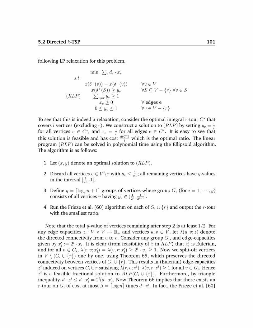
5.2 Directed k-TSP 101
following LP relaxation for this problem.
min∑
e de · xes.t.
x(δ+(v)) = x(δ−(v)) ∀v ∈ Vx(δ+(S)) ≥ yv ∀S ⊆ V − r ∀v ∈ S
(RLP )∑
v 6=r yv ≥ 1
xe ≥ 0 ∀ edges e0 ≤ yv ≤ 1 ∀v ∈ V − r
To see that this is indeed a relaxation, consider the optimal integral r-tour C∗ thatcovers l vertices (excluding r). We construct a solution to (RLP ) by setting yv = 1
l
for all vertices v ∈ C∗, and xe = 1l
for all edges e ∈ C∗. It is easy to see thatthis solution is feasible and has cost d(C∗)
lwhich is the optimal ratio. The linear
program (RLP ) can be solved in polynomial time using the Ellipsoid algorithm.The algorithm is as follows:
1. Let (x, y) denote an optimal solution to (RLP ).
2. Discard all vertices v ∈ V \r with yv ≤ 12n
; all remaining vertices have y-valuesin the interval [ 1
2n, 1].
3. Define g = dlog2 n + 1e groups of vertices where group Gi (for i = 1, · · · , g)consists of all vertices v having yv ∈ ( 1
2i, 1
2i−1 ].
4. Run the Frieze et al. [60] algorithm on each of Gi ∪ r and output the r-tourwith the smallest ratio.
Note that the total y-value of vertices remaining after step 2 is at least 1/2. Forany edge capacities z : V × V → R+ and vertices u, v ∈ V , let λ(u, v; z) denotethe directed connectivity from u to v. Consider any group Gi, and edge-capacitiesgiven by x′i := 2i · xi. It is clear (from feasibility of x in RLP ) that x′i is Eulerian,and for all v ∈ Gi, λ(r, v;x′i) = λ(v, r;x′i) ≥ 2i · yv ≥ 1. Now we split-off verticesin V \ (Gi ∪ r) one by one, using Theorem 65, which preserves the directedconnectivity between vertices of Gi ∪ r. This results in (Eulerian) edge-capacitieszi induced on vertices Gi∪ r satisfying λ(r, v; zi), λ(v, r; zi) ≥ 1 for all v ∈ Gi. Hencezi is a feasible fractional solution to ALP (Gi ∪ r). Furthermore, by triangleinequality, d · zi ≤ d · x′i = 2i(d · x). Now Theorem 66 implies that there exists anr-tour on Gi of cost at most β = dlog ne times d · zi. In fact, the Frieze et al. [60]
102 Chapter 5: VRPs on Asymmetric Metrics
algorithm applied on Gi + r produces such a tour. We now claim that one of ther-tours found in step 4 (over all i = 1, · · · g) has a small ratio:
g
mini=1
β(d · zi)|Gi|
≤g
mini=1
2iβ(d · x)
|Gi|≤ β
∑gi=1 d · x∑g
i=1 |Gi|/2i≤ 4gβ · (d · x)
The last inequality follows from the fact that there is a total y-weight of at least1/2 after step 2, so 1
2≤ ∑v 6=r yv ≤
∑gi=1
12i−1 |Gi| = 2
∑gi=1
|Gi|2i
. Thus we have a4gβ = O(log2 n) approximation algorithm for minimum ratio ATSP.
5.2.3 Algorithm for Directed k-TSP
We now describe how minimum ratio ATSP can be used to obtain an approximationalgorithm for the directed k-TSP problem.
Theorem 70. There is a polynomial time O(log2 n · log k) approximation algorithmfor the directed k-TSP problem.
Proof: We use the α = O(log2 n)-approximation algorithm for the related minimumratio ATSP problem. Let OPT denote the optimal value of the directed k-TSPinstance. By performing binary search, we may assume that we know the value ofOPT within a factor 2. We only consider vertices v ∈ V satisfying d(r, v), d(v, r) ≤OPT; this does not affect the optimal solution. Then we invoke the minimum ratioATSP algorithm repeatedly (each time restricted to the currently uncovered vertices)until the total number of covered vertices t ≥ k
2. Note that for every instance of the
ratio problem that we solve, there is a feasible solution of ratio ≤ 2·OPTk
(namely,the optimal k-TSP tour covering at least k/2 residual vertices). Thus we obtainan r-tour on t ≥ k
2vertices having ratio ≤ 2α·OPT
k; so the length of this r-tour is
at most 2αt·OPTk
. Now, we split this r-tour into l = d2tke di-paths, each containing
at least tl≥ k
4vertices (this can be done in a greedy fashion). By averaging, the
minimum length di-path in this collection has length at most 2αtOPT/kl
≤ α · OPT.Joining the first and last vertices in this di-path to r, we obtain an r-tour containingat least k
4vertices, of length at most (α+ 2) ·OPT. So we get an (O(α), 4) bi-criteria
approximation for directed k-TSP. This algorithm can now be used as follows. Untilat least k vertices are covered, do:
• Let k′ denote the number of vertices covered so far; run the bi-criteria approx-imation algorithm with a target of k − k′, restricted to currently uncoveredvertices.
5.3 Directed Orienteering 103
A standard set cover based analysis implies that this is an O(α · log k)-approximationalgorithm for directed k-TSP.
5.3 Directed Orienteering
In this section, we consider the orienteering problem in asymmetric metrics. Weconsider a slightly more general version than the definition in Section 5.1. In thedirected orienteering problem, we are given metric (V, d), length bound D, origins ∈ V and destination t ∈ V ; the goal is to compute an s− t directed path that haslength at most D and maximizes the number of vertices visited. A closely relatedproblem is directed k-path: given metric (V, d), origin s, destination t, and a targetk, find an s-t directed path of minimum length that visits at least k other vertices.Note that directed k-path reduces to directed k-TSP when s = t.
The algorithm for directed orienteering is based on the following sequenceof reductions: directed orienteering to ‘directed minimum excess’ (Theorem 73),directed minimum excess to directed k-path (Theorem 72), and directed k-path tominimum ratio ATSP (Theorem 71). The first two reductions above are identical tothe corresponding reductions for undirected orienteering in Blum et al. [17] andBansal et al. [13]. We prove the following bi-criteria approximation guarantee fordirected k-path.
Theorem 71. A ρ-approximation algorithm for minimum ratio ATSP implies a (3, 4ρ)bi-criteria approximation algorithm for the directed k-path problem.
Proof: We assume (by performing a binary search) that we know the optimal valueOPT of the directed k-path instance within a constant factor, and let G denote thedirected graph corresponding to metric (V, d) (which has an edge of length d(u, v)from u to v for every pair of vertices u, v ∈ V ). We modify graph G to obtain graphH as follows: (a) discard all vertices v such that d(s, v) > OPT or d(v, t) > OPT;and (b) add an extra edge from t to s of length OPT. In the rest of this proof, werefer to the shortest path metric induced by H as (V, l). Note that each tour inmetric l corresponds to a tour in graph H (using shortest paths in H for each metricedge); below, any tour in metric l will refer to the corresponding tour in graph H.Since there is an s-t path of length OPT (in metric d) covering k vertices, appendingthe (t, s) edge, we have an s-tour σ∗ of length at most 2 ·OPT (in metric l) coveringk + 1 vertices.
104 Chapter 5: VRPs on Asymmetric Metrics
Now, we run the minimum ratio ATSP algorithm with root s in metric l repeatedlyuntil either (1) k
2vertices are covered and the extra (t, s) edge is never used in the
current tour (in graph H); or (2) the extra (t, s) edge is used for the first time inthe current tour (in H). Let σ be the s-tour obtained (in graph H) at the end of thisiteration, and h the number of vertices covered. Note that each s-tour added in asingle call to minimum ratio ATSP, may use the extra (t, s) edge at most once (byan averaging argument). So in case (1), the (t, s) edge is absent in σ, and in case(2), the (t, s) edge is used exactly once and it is the last edge in σ. Note also thatduring each call of minimum ratio ATSP, there is a feasible solution of ratio 2OPT
k
(σ∗ restricted to the remaining vertices); so the ratio of the s-tour σ, l(σ)h≤ ρ · 2OPT
k.
From σ we now obtain a feasible s-t path τ in metric d as follows. In case (1), adda direct (s, t) edge: τ = σ · (s, t); in case (2), remove the only copy of the extra(t, s) edge (occurring at the end of σ): τ = σ \ (t, s). In either case, s-t path τcontains h vertices and has length d(τ) ≤ 2ρh
kOPT + OPT. Note that in case (1),
h ≥ k2; and in case (2), since the extra (t, s) edge is used, OPT
h≤ l(σ)
h≤ 2ρOPT
k, so
h ≥ k2ρ
. Hence in either case, τ contains h ≥ k2ρ
vertices and d(τ) ≤ 4ρhk
OPT. Wenow greedily split τ into maximal paths, each of which has length at most OPT; thenumber of subpaths obtained is at most d(τ)
OPT≤ 4ρh
k. So one of these paths contains
at least h/(4ρhk
) = k4ρ
vertices. Adding direct edges from s to the first vertex on thispath and from the last vertex on this path to t, we obtain an s-t path of length atmost 3 · OPT containing at least k
4ρvertices.
As in Blum et al. [17], we define the excess of an s-t di-path as the difference ofthe path length and the shortest path distance from s to t. The directed minimumexcess problem is defined as follows: given an asymmetric metric (V, d), origin (s)and destination (t) vertices, and a target k, find an s-t di-path of minimum excessthat visits at least k other vertices. The next two theorems together reduce thedirected orienteering problem to the directed k-path problem, for which we justobtained an approximation algorithm.
Theorem 72 (Blum et al. [17]). An (α, β) bi-criteria approximation algorithm forthe directed k-path problem implies a (2α− 1, β) bi-criteria approximation algorithmfor the directed minimum excess problem.
Theorem 73 (Bansal et al. [13]). An (α, β) bi-criteria approximation algorithm forthe directed minimum excess problem implies an dαe · β approximation algorithm forthe directed orienteering problem.
The proofs of Theorems 72 and 73 are identical to the corresponding proofs inthe undirected setting, and are not repeated here. The only difference from the
5.4 Directed Minimum Latency 105
undirected case is that we consider bi-criteria guarantees for the directed k-pathand minimum excess problems. We now obtain a result that relates the directedorienteering problem and minimum ratio ATSP.
Corollary 74. A ρ-approximation algorithm for the minimum ratio ATSP prob-lem implies an O(ρ)-approximation algorithm for the directed orienteering problem.Conversely, a ρ-approximation algorithm for directed orienteering implies an O(ρ)-approximation algorithm for minimum ratio ATSP.
Proof: The first direction follows directly from Theorems 71,72 and 73. For theother direction, we are given a ρ-approximation algorithm for directed orienteering.Let D denote the length of some minimum ratio tour σ∗, t the last vertex visited byσ∗ (before returning to the root r), and h the number of vertices it covers; so theoptimal ratio is D
h. The algorithm for minimum ratio ATSP first guesses a value D′
such that D′ ≤ D ≤ 2 ·D′, and the last vertex t. Note that we can guess powers oftwo for the value of D′, which gives O(log2(n ·dmax)) possibilities for D′ (where dmaxis the length of the longest edge). Also, the number of possibilities for t is at most n;so the algorithm only makes a polynomial number of guesses. The algorithm thenruns the directed orienteering algorithm with r and t as the start/end vertices and alength bound of 2D′ − d(t, r) ≥ D − d(t, r). Note that removing the last (t, r) edgefrom σ∗ gives a feasible solution to this orienteering instance that covers h vertices.Hence the ρ-approximation algorithm is guaranteed to find an r-t di-path coveringat least h
ρvertices, having length at most 2D′ − d(t, r). Now, adding the (t, r) edge
to this path gives an r-tour of ratio at most 2D′/(hρ) ≤ 2ρD
h.
Corollary 74 and Theorem 69 imply an O(log2 n)-approximation algorithm fordirected orienteering. Furthermore, any improvement in minimum ratio ATSPimplies a corresponding improvement for directed orienteering.
5.4 Directed Minimum Latency
In this section, we present our algorithm for the directed latency problem. First weestablish the equivalence (up to a constant factor) of the ‘tour’ and ‘path’ versions ofthe latency problem. Recall that Path latency involves computing a spanning r-pathπ that minimizes
∑v∈V d
π(r, v) (here dπ(r, r) = 0); and Tour latency involves findinga spanning r-tour τ that minimizes
∑v∈V d
τ (r, v) (here dτ (r, r) = d(τ)).
106 Chapter 5: VRPs on Asymmetric Metrics
Theorem 75. The approximability of the path and tour versions of directed latencyare within a factor 4 of each other.
Proof: Reducing Tour-latency to Path-latency. We first show that any approxima-tion algorithm for path-latency implies the same guarantee for tour-latency. Modifythe given metric (V, d) (for tour-latency) by adding a new vertex r′ with distancesto vertices V as follows: d(v, r′) = d(v, r) and d(r′, v) =∞ for all v ∈ V . It is clearthat any spanning r-path in the modified metric corresponds to a spanning r-tour inthe original metric followed by edge (r, r′) (which has length 0). Hence there is acorrespondence between solutions to tour-latency and path-latency, that maintainsthe objective value.
Reducing Path-latency to Tour-latency. Let A be any α-approximation algorithmfor tour-latency (we assume α ≤ n). Set β = d4αe + 1 and define a new metric(V , d) which is obtained from (V, d) by making β copies of each vertex in V \ r (foreach v ∈ V \ r, all its copies in V are at distance 0 from each other). Let ˜pLat(resp. pLat) denote the optimal value of path-latency on d (resp. d); note that
˜pLat = β · pLat. We assume (by scaling) that the smallest non-zero distance in d is 1,and that there is a finite length spanning r-path in metric d (otherwise the latencyproblem is trivial); so pLat ≤ n2dmax where dmax is the maximum finite distance ind. We further modify metric d by adding dummy edges of length L (exact value tobe set later) from each vertex in V \ r to r, and let l denote the shortest path metricon this modified graph. Note that the optimal value of tour-latency on metric l istLat ≤ 2 · ˜pLat + L. The algorithm for path-latency on d is as follows.
• For each 0 ≤ i ≤ lg(βn2dmax) do:
1. Set L← 2i and l to be the metric as defined above.
2. Run algorithm A for tour-latency on l to get tour τ . Let π denote theportion of τ until the first usage of a dummy edge.
3. If π visits at least one copy of each vertex in V , consider this as a feasiblesolution to path-latency on d; otherwise skip this iteration.
• Output the best path-latency solution encountered in Step 3 above.
Note that since 1 ≤ ˜pLat ≤ βn2dmax, there is an iteration where ˜pLat ≤ L =2i ≤ 2 · ˜pLat. We now argue that in this iteration i, the above algorithm gets afeasible solution in Step 3 with path-latency value (on metric d) at most 4α · pLat.
5.4 Directed Minimum Latency 107
The tour τ found by algorithm A has latency (in metric l) Lat(τ) ≤ α · tLat ≤α(2 · ˜pLat + L) ≤ 4α · ˜pLat. If x denotes the number of unvisited vertices of V in π(i.e. when a dummy edge is used for the first time in τ) then Lat(τ) ≥ L · x; hencex ≤ Lat(τ)/L ≤ 4α · ˜pLat/L ≤ 4α < β. Since V has β copies of each vertex of V , πvisits at least one copy of each V -vertex: so Step 3 records π as a potential solution.We modify τ so that it visits all copies of each V -vertex the first time some copy isvisited: this only reduces the latency of τ . After this modification, note that dummyedges are used in τ only after all vertices V are visited: in other words, τ inducesa path-latency solution on metric (V , d) of latency value Lat(τ) ≤ 4α · ˜pLat, thatdoes not use any dummy edge. Hence the corresponding solution π in metric (V, d)has latency Lat(π) = 1
βLat(τ) ≤ 1
β4α · ˜pLat = 4α · pLat. Thus the best solution to
path-latency on d obtained over all iterations has value at most 4α · pLat, and wehave a 4α approximation algorithm.
The next proposition shows that the directed latency problem is at least as hardto approximate as the Asymmetric Traveling Salesman Problem.
Proposition 76. An α-approximation for directed latency (path version) implies a4α-approximation for ATSP. This reduction also holds in the special case of metricsinduced by unweighted digraphs.
Proof: We only present the reduction for unweighted metrics (the general case isidentical). Let A be an α-approximation algorithm for the (path version) directedlatency on unweighted metrics, and G = (V,E) any n-vertex digraph that induces ashortest-path metric. We show how A can be used to obtain a 4α approximationfor ATSP on G. Pick some root r ∈ V and modify G by adding to it a directed pathof n new vertices U originating at r: let H be the graph so obtained. A candidatesolution for latency on H first visits the vertices V along the optimal ATSP touron G and then visits U along the new path: this implies that the optimal latencyon H, Lat∗(H) ≤ 2n(Tsp∗(G) + n) where Tsp∗(G) is the optimal value of ATSP onG. Note that Tsp∗ ≥ n (G has n vertices), and so Lat∗(H) ≤ 4nTsp∗(G). Notealso that any spanning r-path in H must first visit all the vertices V in some r-tour(that lies in graph G) and then the vertices U along the new path. Since thereare n vertices (those in U) that appear after the spanning tour on G, we haveLat∗(H) ≥ n · Tsp∗(G). Thus we have 1
4nLat∗(H) ≤ Tsp∗(G) ≤ 1
nLat∗(H), which
implies the proposition.
Before presenting the algorithm for directed latency, we define and describe anLP relaxation for the Asymmetric Traveling Salesman Path (ATSP-path) problem.
108 Chapter 5: VRPs on Asymmetric Metrics
This LP is used in the algorithm for directed latency.
ATSP-path. Here we are given a directed metric (V, d) and specified start and endvertices s, t ∈ V . The goal is to compute the minimum length s− t path that visits allthe vertices. As mentioned earlier, it is known that the approximability of ATSP-pathand ATSP are equal (up to a constant factor) [53]. We are concerned with thefollowing LP relaxation of the ATSP-path problem.
min∑
e de · xes.t.
x(δ+(u)) = x(δ−(u)) ∀u ∈ V − s, tx(δ+(s)) = x(δ−(t)) = 1
(ATSP − path) x(δ−(s)) = x(δ+(t)) = 0x(δ−(S)) ≥ 2
3∀u ⊆ S ⊆ V \ s, ∀u ∈ V
xe ≥ 0 ∀ arcs e
The most natural LP relaxation for ATSP-path would have a one in the right-hand-side of the cut constraints, instead of 2
3as above. The above LP further relaxes
the cut-constraints, and is still a valid relaxation of the problem. The precise valuein the right-hand-side of the cut constraints is not important for our application:we only require it to be some constant strictly between 1
2and 1. Note that if the
right-hand-side of the cut constraints is 12
then the LP has infinite integrality gap,as shown by an instance consisting of two vertex disjoint paths from s to t. In therest of this section, we let ρ denote the integrality gap of this LP. We study this LPfurther in Section 5.5, where we obtain an upper bound ρ = O(
√n).
5.4.1 Algorithm for directed latency
We assume (by scaling) that the smallest non-zero distance in the given metric(V, d) is one, and let dmax denote the largest finite distance. The algorithm fordirected latency is also given a parameter Ω( 1
logn) ≤ ε < 1: it produces an O(ρ · nε
ε3)
approximation in nO(1/ε) time.
For the given instance of directed latency on metric (V, d) with root r, let πdenote an optimal latency path, L = d(π) its length, and OPT its total latency. Notethat 1 ≤ L ≤ n · dmax. For any two vertices u, v ∈ V , recall that dπ(u, v) denotes thelength along path π from u to v; note that dπ(u, v) is finite only if u appears beforev on path π. The algorithm first guesses the length L (within factor 2) and the
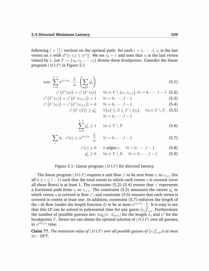
5.4 Directed Minimum Latency 109
following l = d1εe vertices on the optimal path: for each i = 1, · · · , l, vi is the last
vertex on π with dπ(r, vi) ≤ niε Ln. We set v0 = r and note that vl is the last vertex
visited by π. Let F := v0, v1, · · · , vl denote these breakpoints. Consider the linearprogram (MLP ) in Figure 5.1
minl−1∑i=0
n(i+1)ε · Ln·(∑u/∈F
yiu
)(5.1)
zi(δ+(u)
)= zi
(δ−(u)
)∀u ∈ V \ vi, vi+1, ∀i = 0, · · · , l − 1 (5.2)
zi(δ+(vi)
)= zi
(δ−(vi+1)
)= 1 ∀i = 0, · · · , l − 1 (5.3)
zi(δ−(vi)
)= zi
(δ+(vi+1)
)= 0 ∀i = 0, · · · , l − 1 (5.4)
zi(δ−(S)
)≥ yiu ∀u ⊆ S ⊆ V \ vi, ∀u ∈ V \ F, (5.5)
∀i = 0, · · · , l − 1l−1∑i=0
yiu ≥ 1 ∀u ∈ V \ F (5.6)
∑e
de · zi(e) ≤ n(i+1)ε · Ln
∀i = 0, · · · , l − 1 (5.7)
zi(e) ≥ 0 ∀ edges e, ∀i = 0, · · · , l − 1 (5.8)yiu ≥ 0 ∀u ∈ V \ F, ∀i = 0, · · · , l − 1 (5.9)
Figure 5.1: Linear program (MLP ) for directed latency.
The linear program (MLP ) requires a unit flow zi to be sent from vi to vi+1 (forall 0 ≤ i ≤ l − 1) such that the total extent to which each vertex u is covered (overall these flows) is at least 1. The constraints (5.2)-(5.4) ensure that zi representsa fractional path from vi to vi+1. The constraint (5.5) measures the extent yiu towhich vertex u is covered in flow zi, and constraint (5.6) ensures that each vertex iscovered to extent at least one. In addition, constraint (5.7) enforces the length ofthe i-th flow (under the length function d) to be at most n(i+1)ε · L
n. It is easy to see
that this LP can be solved in polynomial time for any guess vili=1. Furthermorethe number of possible guesses are: log2(n · dmax) for the length L, and nl for thebreakpoints F . Hence we can obtain the optimal solution of (MLP ) over all guesses,in nO(1/ε) time.
Claim 77. The minimum value of (MLP ) over all possible guesses of vili=0 is at most2nε · OPT.
110 Chapter 5: VRPs on Asymmetric Metrics
Proof: This claim is straightforward, based on the correct guesses from an optimalpath. Recall that π is an optimal latency path for the given instance. One ofthe guesses of the vertices vili=0 satisfies the following condition: each vi (fori = 1, · · · , l) is the last vertex on π with dπ(s, vi) ≤ niε L
n. For each i = 0, · · · , l − 1,
define Oi to be the set of vertices that are visited between vi and vi+1 in path π. Let zi
denote the (integral) edge values corresponding to path π restricted to the verticesOi ∪ vi, vi+1; note that the cost of this flow d · zi ≤ dπ(r, vi+1) ≤ n(i+1)ε L
n. Also set
yiu = 1 for u ∈ Oi and 0 otherwise, for all i = 0, · · · , l − 1. Note that each vertexin V \ vili=0 appears in some set Oi, and each zi supports unit flow from vi to allvertices in Oi; hence this integral solution zi, yil−1
i=0 is feasible for (MLP ). The costof this solution is
∑l−1i=0 n
(i+1)ε Ln· |Oi| ≤ nεL+ nε
∑l−1i=1 n
iε Ln· |Oi| ≤ 2nε · OPT, since
|O0| ≤ n, L ≤ OPT, and each vertex u ∈ Oi (for i = 1, · · · , l− 1) has dπ(r, u) > niε Ln
.
We now assume that we have an optimal fractional solution zi, yil−1i=0 to (MLP )
over all guesses (with objective value as in Claim 77), and show how to round it toobtain vi − vi+1 paths for each i = 0, · · · , l − 1, which when concatenated give riseto one r-path having a small latency objective. We say that a vertex u is well-coveredby flow zi if yiu ≥ 1
4l. We partition the vertices V \ F into two parts: V1 consists of
those vertices that are well-covered for at least two values of i ∈ 0, 1, · · · , l, andV2 consists of all other vertices (i.e. well-covered for only one i ∈ 0, 1, · · · , l. Notethat each vertex in V2 is in fact covered by some flow zi to the extent at least 3
4. See
also Figure7.1.
In the next two subsections, we give algorithms to service each of V1 and V2
separately using local paths, and then in Section 5.4.4 we show to stitch all the localpaths into a single spanning r-path.
5.4.2 Servicing vertices V1
We partition V1 into l parts as follows: Ui (for i = 0, · · · , l − 1) consists of thosevertices of V1 that are well-covered by zi but not well-covered by any flow zj forj > i. Each set Ui is serviced separately by means of a suitable ATSP solution onUi ∪ vi (see Lemma 79): this step requires a bound on the length of back-arcsfrom Ui-vertices to vi, which is ensured by the next claim.
Claim 78. For each vertex w ∈ Ui, d(w, vi) ≤ 8l · niε Ln.
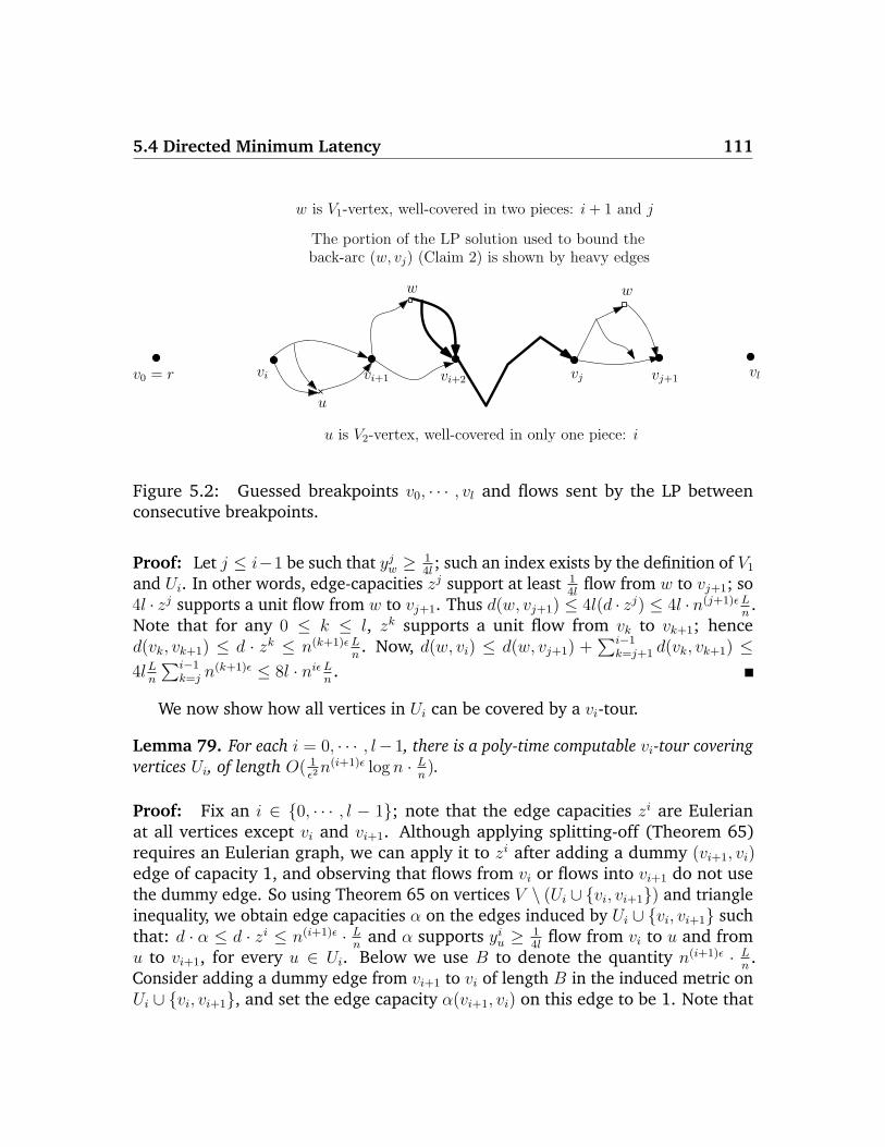
5.4 Directed Minimum Latency 111
vi+2v0 = r
u
vjvi vi+1 vj+1vl
ww
u is V2-vertex, well-covered in only one piece: i
w is V1-vertex, well-covered in two pieces: i + 1 and j
The portion of the LP solution used to bound theback-arc (w, vj) (Claim 2) is shown by heavy edges
Figure 5.2: Guessed breakpoints v0, · · · , vl and flows sent by the LP betweenconsecutive breakpoints.
Proof: Let j ≤ i−1 be such that yjw ≥ 14l
; such an index exists by the definition of V1
and Ui. In other words, edge-capacities zj support at least 14l
flow from w to vj+1; so4l · zj supports a unit flow from w to vj+1. Thus d(w, vj+1) ≤ 4l(d · zj) ≤ 4l · n(j+1)ε L
n.
Note that for any 0 ≤ k ≤ l, zk supports a unit flow from vk to vk+1; henced(vk, vk+1) ≤ d · zk ≤ n(k+1)ε L
n. Now, d(w, vi) ≤ d(w, vj+1) +
∑i−1k=j+1 d(vk, vk+1) ≤
4lLn
∑i−1k=j n
(k+1)ε ≤ 8l · niε Ln.
We now show how all vertices in Ui can be covered by a vi-tour.
Lemma 79. For each i = 0, · · · , l− 1, there is a poly-time computable vi-tour coveringvertices Ui, of length O( 1
ε2n(i+1)ε log n · L
n).
Proof: Fix an i ∈ 0, · · · , l − 1; note that the edge capacities zi are Eulerianat all vertices except vi and vi+1. Although applying splitting-off (Theorem 65)requires an Eulerian graph, we can apply it to zi after adding a dummy (vi+1, vi)edge of capacity 1, and observing that flows from vi or flows into vi+1 do not usethe dummy edge. So using Theorem 65 on vertices V \ (Ui ∪ vi, vi+1) and triangleinequality, we obtain edge capacities α on the edges induced by Ui ∪ vi, vi+1 suchthat: d · α ≤ d · zi ≤ n(i+1)ε · L
nand α supports yiu ≥ 1
4lflow from vi to u and from
u to vi+1, for every u ∈ Ui. Below we use B to denote the quantity n(i+1)ε · Ln.
Consider adding a dummy edge from vi+1 to vi of length B in the induced metric onUi ∪ vi, vi+1, and set the edge capacity α(vi+1, vi) on this edge to be 1. Note that
112 Chapter 5: VRPs on Asymmetric Metrics
α is Eulerian, has total cost at most 2B, and every non-trivial cut has value at leastminyiu : u ∈ Ui ≥ 1
4l. So scaling α uniformly by 4l, we obtain a fractional feasible
solution to ATSP on the vertices Ui ∪ vi, vi+1 (in the modified metric), having costat most 8l ·B. Since the Frieze et al. [60] algorithm computes an integral tour oflength at most O(log n) times any fractional feasible solution (see Williamson [156]or Theorem 68), we obtain a vi-tour τ on the modified metric of length at mostO(l log n) · B. Since the dummy (vi+1, vi) edge has length B, it may be used atmost O(l log n) times in τ . So removing all occurrences of this dummy edge givesa set of O(l log n) paths from vi to vi+1 in the original metric, that together coverUi. Ignoring vertex vi+1 and inserting the direct edge to vi from the last Ui vertexin each of these paths gives us a vi-tour covering Ui. Finally note that each of theedges to vi inserted above has length O(l · niε)L
n= O(l) · B (from Claim 78), and
the number of edges inserted is O(l log n). So the length of this vi-tour is at mostO(l log n) ·B +O(l2 log n) ·B = O( 1
ε2n(i+1)ε log n · L
n).
5.4.3 Servicing vertices V2
We partition vertices in V2 into W0, · · · ,Wl−1, where each Wi contains the verticesin V2 that are well-covered by zi. As noted earlier, each vertex u ∈ Wi in facthas yiu ≥ 3
4> 2
3. We now consider any particular Wi and obtain a vi − vi+1 path
covering the vertices of Wi. Vertices in Wi are covered by a fractional vi − vi+1
path as follows. Splitting off vertices V \ (Wi ∪ vi, vi+1) in the fractional solutionzi gives us edge capacities β in the metric induced on Wi ∪ vi, vi+1, such that:β supports at least 2
3flow from vi to u and from u to vi+1 for all u ∈ Wi, and
d ·β ≤ d · zi (this is similar to how edge-capacities α were obtained in Lemma 5.4.2).Note that β is a fractional feasible solution to the LP relaxation (ATSP − path)for the ATSP-path instance on the metric induced by Wi ∪ vi, vi+1 with start-vertex vi and end-vertex vi+1. So if ρ denotes the (constructive) integrality gap of(ATSP − path), we can obtain an integral vi-vi+1 path that spans Wi, having lengthat most ρ(d · β) ≤ ρ(d · zi) ≤ ρn(i+1)ε L
n. This requires a polynomial time algorithm
that computes an integral path of length at most ρ times the LP value; Howevereven a non-constructive proof of integrality gap ρ′ implies a constructive integralitygap ρ = O(ρ′ log n), using the algorithm in Chekuri and Pal [32]. So we obtain:
Lemma 80. For each i = 0, · · · , l − 1, there is a poly-time computable vi-vi+1 pathcovering Wi of length at most ρ · n(i+1)ε L
n.
5.5 Integrality Gap of ATSP-path 113
5.4.4 Stitching the local paths
We now stitch the vi-tours that service V1 (Lemma 79) and the vi − vi+1 paths thatservice V2 (Lemma 80), to obtain a single r-path that covers all vertices. For eachi = 0, · · · , l − 1, let πi denote the vi-tour servicing Ui, and let τi denote the vi − vi+1
path servicing Wi. The final r-path that the algorithm outputs is the concatenationτ ∗ = π0 · τ0 · π1 · · · πl−1 · τl−1. From Lemmas 79 and 80, it follows that for all0 ≤ i ≤ l− 1, d(πi) ≤ O( 1
ε2log n) · n(i+1)ε L
nand d(τi) ≤ O(ρ) · n(i+1)ε L
n. So the length
of τ ∗ from r until all vertices of Ui∪Wi are covered is at most O(ρ+ 1ε2
log n) ·n(i+1)ε Ln
(as ε ≥ Ω( 1logn
)). This implies that the total latency of vertices in Ui ∪Wi along pathτ ∗ is at most O(ρ+ 1
ε2log n) · n(i+1)ε L
n· (|Wi|+ |Ui|).
Moreover, the contribution of each vertex in Ui (resp., Wi) to the LP objective isat least 1
4l· n(i+1)ε L
n(resp., 3
4· n(i+1)ε L
n). Thus the contribution of Ui ∪Wi to the LP
objective is at least 14l· n(i+1)ε L
n· (|Wi|+ |Ui|). Using the upper bound on the latency
along τ ∗ for Ui ∪Wi, and summing over all i, we obtain that the total latency alongτ ∗ is at most O(1
ερ+ 1
ε3log n) times the optimal value of (MLP ). From Claim 77, it
now follows that the latency of τ ∗ is O(1ερ+ 1
ε3log n)nε · OPT.
Theorem 81. For any Ω( 1logn
) < ε < 1, there is an O(ρ+lognε3· nε)-approximation
algorithm for directed latency, that runs in time nO(1/ε), where ρ is the integrality gapof the LP (ATSP − path). Using ρ = O(
√n), we have a polynomial time O(n
12
+ε)approximation algorithm for any fixed ε > 0.
We prove the bound ρ = O(√n) in the next section. A bound of ρ = O(log n)
on the integrality gap of (ATSP − path) would imply that this algorithm is aquasi-polynomial time O(log4 n) approximation for directed latency.
5.5 Integrality Gap of ATSP-path
In this section we prove an upper bound of ρ = O(√n) on the integrality gap of the
linear relaxation (ATSP − path) (c.f. Section 5.4). Even for the seemingly strongerLP with one in the right-hand-side of the cut constraints, the best bound on theintegrality gap we can obtain is O(
√n): this follows from the cycle-cover based
algorithm of Lam and Newmann [103]. As mentioned in Chekuri and Pal [32], it isunclear whether their O(log n)-approximation can be used to bound the integralitygap of such a linear program. In this section, we present a rounding algorithm forthe weaker LP (ATSP − path), which shows ρ = O(
√n). Our algorithm is similar
114 Chapter 5: VRPs on Asymmetric Metrics
to the ATSP-path algorithm of Lam and Newmann [103] and the ATSP algorithmof Frieze et al. [60]; but it needs some more work as we compare the algorithm’ssolution against a fractional solution to (ATSP − path). We note that the proofholds for any fixed constant 1
2< c < 1 in the right-hand-side of the cut-constraints
of (ATSP − path). Furthermore the reduction from directed latency (Theorem 81)also holds for any constant 1
2< c < 1. However if c ≤ 1
2, the integrality gap of the
LP (ATSP − path) is infinite (eg., a graph consisting of two vertex disjoint pathsfrom s to t).
Let x be any feasible solution to (ATSP − path). We now show how x can berounded to obtain an integral path spanning all vertices, of total length O(
√n)(d ·x).
Let N denote a network (corresponding to the directed metric) on vertices V withedges between all pairs of vertices, where the cost of each edge equals its metriclength and the capacity of each edge is ∞. An extra (t, s) edge of zero cost andcapacity three is added to N . The rounding algorithm for x is as follows.
1. Initialize the set of representatives R ← V \ s, t, and the current integralsolution σ = ∅.
2. While R 6= ∅, do:
(a) Compute a minimum cost circulation C in N [R ∪ s, t] (the network Ninduced on R ∪ s, t) that sends at least 2 units of flow through eachvertex in R. Note that any circulation (in particular C) can be expressedas an edge-disjoint sum of cycles.
(b) Repeatedly extract from C all cycles that do not use the extra edge (t, s),to obtain circulation A ⊆ C. Let R′ ⊆ R be the set of R-vertices that havedegree at least 1 in A.
(c) Let B = C \ A; note that B is also a circulation and each cycle in it usesedge (t, s).
(d) If |R′| ≥ √n, do:
i. Set σ ← σ ∪ A.ii. Modify R by dropping all but one R′-vertex from each strong compo-
nent of A.
(e) If |R′| < √n, do:
i. Take an Euler tour on B and remove all (at most 3) occurrences ofedge (t, s) to obtain s-t paths P1, P2, P3.
5.5 Integrality Gap of ATSP-path 115
ii. Restrict each path P1, P2, P3 to vertices in R \R′ by short-cutting overR′-vertices, to obtain paths P1, P2, P3.
iii. Take a topological ordering s = w1, w2, · · · , wh = t of vertices (R \R′) ∪ s, t relative to the edge-set P1 ∪ P2 ∪ P3.
iv. Set σ ← σ ∪ (wj, wj+1) : 1 ≤ j ≤ h− 1.v. Repeat for each vertex u ∈ R′: find an edge (w,w′) ∈ σ such thatx supports 1
6flow from w to u and from u to w′, and modify σ ←
(σ \ (w,w′)) ∪ (w, u), (u,w′).vi. Set R← ∅.
3. Output any spanning s-t walk in σ.
We now show the correctness and performance guarantee of the roundingalgorithm. We first bound the cost of the circulation obtained in Step 2a during anyiteration.
Claim 82. For any R ⊆ V \s, t, the minimum cost circulation C computed in step 2ahas cost at most 3(d · x).
Proof: The edge values x define a fractional s− t path in network N . Extend x tobe a (fractional) circulation by setting x(t, s) = 1. We can now apply splitting-off(Theorem 65) on each vertex in V \ R \ s, t, to obtain capacities x′ in networkN [R ∪ s, t], such that every pairwise connectivity is preserved and (by triangleinequality) d · x′ ≤ d · x. Note that since neither s nor t is split-off, the extra (t, s)edge is not modified in the splitting-off steps. So x′ supports 2
3flow from s to each
vertex in R; this implies that 3x′ is a feasible fractional solution to the circulationinstance solved in step 2a (note that x′(t, s) remains 1, so solution 3x′ satisfiesthe capacity of edge (t, s)). Finally, note that the linear relaxation for circulationis integral (c.f. Nemhauser and Wolsey [119]). So the minimum cost (integral)circulation computed in step 2a has cost at most 3d · x′ ≤ 3d · x.
Note that each time step 2d is executed, |R| decreases by at least√n/2 (each
strong component in A has at least 2 vertices); so there are at most O(√n) such
iterations and the cost of σ due to additions in this step is O(√n)(d · x) (using
Claim 82). Step 2e is executed at most once (at the end); the next claim shows thatthis step is well defined and bounds the cost incurred.
Claim 83. In step 2(e)iii, there exists a topological ordering w1, · · · , wh of (R \R′) ∪s, t w.r.t. edges P1∪P2∪P3. Furthermore, (wj, wj+1) : 1 ≤ j ≤ h−1 ⊆ P1∪P2∪P3.
116 Chapter 5: VRPs on Asymmetric Metrics
Proof: Note that any cycle in P1 ∪ P2 ∪ P3 is a cycle in B that does not use edge(t, s), which is not possible by the construction of B (every cycle in B uses edge(t, s)); so P1 ∪ P2 ∪ P3 is acyclic. It is clear that if P1 ∪ P2 ∪ P3 contains a cycle,so does P1 ∪ P2 ∪ P3 (each path Pi is obtained by short-cutting the correspondingpath Pi). Hence P1 ∪ P2 ∪ P3 is also acyclic, and there is a topological ordering (sayw1, · · · , wh) of (R \ R′) ∪ s, t relative to edges P1 ∪ P2 ∪ P3. We now prove thesecond part of the claim. In circulation C, each vertex of R has at least 2 units offlow through it; but vertices R \ R′ are not covered (even to an extent 1) in thecirculation A. So each vertex of R\R′ is covered to extent at least 2 in circulation B,and hence in P1 ∪ P2 ∪ P3. In other words, each vertex of R \R′ appears on at leasttwo of the three s− t paths P1, P2, P3. This also implies that (after the short-cutting)each R \R′ vertex appears on at least two of the three s− t paths P1, P2, P3. Nowobserve that for each consecutive pair (wj, wj+1) (1 ≤ j ≤ h− 1) in the topologicalorder, there is a common path Pk (for some k = 1, 2, 3) that contains both wj andwj+1. Furthermore, in Pk, wj and wj+1 are consecutive in that order (otherwise,the topological order would contain a back edge!). Thus each edge (wj, wj+1) (for1 ≤ j ≤ h− 1) is present in P1 ∪ P2 ∪ P3, and we obtain the claim.
We also need the following claim to bound the cost of insertions in step 2(e)v.
Claim 84. For any two vertices u′, u′′ ∈ V , if λ(u′, u′′;x) (resp. λ(u′′, u′;x)) denotesthe directed connectivity under x from u′ to u′′ (resp. from u′′ to u′), then λ(u′, u′′;x) +λ(u′′, u′;x) ≥ 1
3.
Proof: If either u′ or u′′ is in s, t, the claim is obvious since for every vertex v, xsupports 2
3flow from s to v and from v to t. Otherwise s, t, u′, u′′ are distinct, and
define capacities x as:
x(v1, v2) =
x(v1, v2) for edges (v1, v2) 6= (t, s)
1 for edge (v1, v2) = (t, s)
Observe that x is Eulerian; now apply Theorem 65 to x and split-off all verticesof V except T = s, t, u′, u′′, and obtain capacities y on the edges induced on T .We have λ(t1, t2; y) = λ(t1, t2; x) for all t1, t2 ∈ T . Note that since neither t nor sis split-off, their degrees in y are unchanged from x, and also y(t, s) ≥ x(t, s) = 1.Since the out-degree of t in x (hence in y) is 1 and yt,s ≥ 1, we have y(t, u′) =y(t, u′′) = 0 and y(t, s) = 1. The capacities y support at least 2
3flow from s to u′; so
y(s, u′) + y(u′′, u′) ≥ 23. Similarly for u′′, we have y(s, u′′) + y(u′, u′′) ≥ 2
3, and adding
these two inequalities we get y(u′, u′′)+y(u′′, u′)+(y(s, u′)+y(s, u′′)) ≥ 43. Note that
5.5 Integrality Gap of ATSP-path 117
y(s, u′) + y(s, u′′) ≤ y(δ+(s)) = x(δ+(s)) = 1 (the degree of s is unchanged in thesplitting-off). So y(u′, u′′) + y(u′′, u′) ≥ 1
3. Since y is obtained from x by a sequence
of splitting-off operations, it follows that x supports flows corresponding to all edgesin y simultaneously. In particular, the following flows are supported disjointly in x:F1 that sends y(u′, u′′) units from u′ to u′′, F2 that sends y(u′′, u′) units from u′′ to u′,and F3 that sends y(t, s) = 1 unit from t to s. Hence the flows F1 and F2 are eachsupported by x and do not use the extra (t, s) edge (since x(δ+(t)) = x(t, s) = 1).This implies that the flows F1 and F2 are both supported by the original capacitiesx (where x(t, s) = 0). Hence λ(u′, u′′;x) + λ(u′′, u′;x) ≥ y(u′, u′′) + y(u′′, u′) ≥ 1
3.
From Claim 83, we obtain that the cost addition in step 2e(iv) is at mostd(P1) + d(P2) + d(P3) ≤ d(P1) + d(P2) + d(P3) ≤ 3(d · x) (from Claim 82). We nowconsider the cost addition to σ in step 2(e)v. Claim 84 implies that for any pairof vertices u′, u′′ ∈ V , x supports 1
6flow either from u′ to u′′ or from u′′ to u′. Also
for every vertex u, x supports 23
flow from s to u and from u to t. Since σ alwayscontains an s− t path in step 2(e)v, there is always some position along this s− tpath to insert any vertex u ∈ R′ as required in step 2(e)v. Furthermore, the costincrease in any such insertion step is at most 12(d · x). Hence the total cost forinserting all the vertices R′ into σ is at most 12|R′|(d · x) = O(
√n)(d · x). Thus the
total cost of σ at the end of the algorithm is O(√n)(d · x). Finally note that σ is
connected (in the undirected sense), Eulerian at all vertices in V \ s, t and hasoutdegree 1 at s. This implies that σ corresponds to a spanning s − t walk. Thiscompletes the proof of the following.
Theorem 85. The integrality gap of (ATSP − path) is at most O(√n).
Credits: The results in this chapter are from “Poly-logarithmic Approximation Al-gorithms for Directed Vehicle Routing Problems” [113] and “The Directed MinimumLatency Problem” [114], obtained jointly with R. Ravi. In independent work, Chekuriet al. [30] also obtained the results on directed orienteering reported here, althoughvia different techniques.

Chapter 6
Permutation Flowshop Scheduling
6.1 Introduction
In the flow shop problem, there are m machines located in a fixed order (say, 1through m), and n jobs each of which consists of a sequence of operations onmachines (in the order 1 through m). For any job j ∈ 1, . . . , n and machinei ∈ 1, . . . ,m the length of the operation of job j on machine i is called itsprocessing time pij. A schedule for the jobs is feasible if (i) each machine processesat most one job at any time; (ii) for each job, its operations on the machines areprocessed in the fixed order 1 through m; and (iii) each operation (of a job on amachine) is processed without interruption. The flow shop problem is a special caseof acyclic job shop scheduling [40, 48], which in turn is a special case of the generaljob shop scheduling [33, 104].
In this chapter, we study the permutation flow shop problem, which is the flowshop problem with the additional constraint that each machine processes all the jobsin the same order. So any feasible schedule to the permutation flow shop problemcorresponds to a permutation of the n jobs. It is well-known [38] that there existsan optimal schedule for the ordinary flow shop problem having the same processingorder (of jobs) on the first two machines and the same processing order on the lasttwo machines. So the permutation flow shop problem is equivalent to the ordinaryflow shop problem for m ≤ 3 machines. However, it is easy to construct an instancewith m = 4 machines where no permutation schedule is optimal for the ordinaryflow shop problem.
Two natural objective functions that are typically considered for scheduling
119
120 Chapter 6: Permutation Flowshop Scheduling
problems are makespan and weighted completion time. The makespan of a scheduleis the completion time of its last job, i.e. maximum completion time among all jobs.For the weighted completion time objective, each job j comes with a weight wj ≥ 0,and the weighted completion time of a schedule is the weighted sum of completiontimes over all jobs.
6.1.1 Preliminaries
An instance of the permutation flow shop problem with m machines and n jobsis given by an m × n matrix P = pi,j | i = 1, · · · ,m, j = 1, · · · , n of processingtimes, where pi,j is the processing time of job j on machine i. We often denotethe set 1, · · · , n of all jobs by [n], and the set 1, · · · ,m of all machines by [m].Any feasible schedule for permutation flow shop corresponds to a permutation ofthe n jobs. Given a permutation π : [n] → [n] of jobs, the complete schedule ofjob-operations on machines can be obtained by running jobs on machines in theorder π while maintaining the minimum possible wait-time between operations.It is convenient to think of π as a mapping from the set of n possible positions tothe set of n jobs. Therefore, π(p) denotes the job located at position p. For anypermutation π of the n jobs and a job j ∈ [n], we use Cπ
j to denote the completiontime of job j under the schedule π; we also denote the makespan of scheduleπ by Cπ
max = maxnj=1 Cπj . Given non-negative weights wjnj=1 for the jobs, the
weighted completion time objective of the schedule corresponding to permutation πis∑n
j=1 wjCπj .
The following are two obvious lower bounds for the permutation flow shopscheduling problem with the makespan objective: maximum job length (denotedl := maxnj=1
∑mi=1 pi,j), and maximum machine load (L := maxmi=1
∑nj=1 pi,j). We
refer to maxl, L as the trivial lower bound. Our algorithms are based on just theselower bounds.
A monotone path (or critical path) in an m×n matrix is defined to be a sequence〈(x1, y1), · · · , (xt, yt)〉 of matrix positions such that (x1, y1) = (1, 1), (xt, yt) = (m,n),and for each 1 ≤ i < t either xi+1 = xi+1 and yi+1 = yi or xi+1 = xi and yi+1 = yi+1.In particular, this definition implies that each monotone path in an m× n matrixconsists of exactly t = m+ n− 1 positions. We denote the set of all monotone pathsin an m× n matrix byMm,n.
A map τ : [n]→ X ∪ ∅ where X ⊆ [m] is called a partial permutation if thereis a subset Y ⊆ [n] with |Y | = |X| such that (i) τ(Y ) = X (τ is a one-to-one map
6.1 Introduction 121
from Y to X); and (ii) τ(z) = ∅ for all z ∈ [n] \ Y . For such a partial permutation τ ,we refer to the set X as its image, denoted Image(τ). A 0-1 m× n matrix Π is calleda permutation matrix if every row and column has at most one entry that is 1 (allother entries are 0s). Note that there is an obvious correspondence between partialpermutations and permutation matrices. In the rest of the paper we will use partialpermutations that map a subset of jobs into a set of machines.
6.1.2 Our Results
We give a simple randomized algorithm (Section 6.2) for minimizing makespan inthe permutation flowshop problem, that achieves an approximation guarantee of2√
minm,n. This guarantee is relative to the trivial lower bounds. The analysisis based on a connection between the permutation flow shop scheduling problemand the longest increasing subsequence problem. Hence we answer an openquestion from Potts et al. [126], by matching algorithmically the Ω(
√minm,n)
gap (between optimal makespan and the trivial lower bound) shown in [126].
We also show how this algorithm can be derandomized to obtain a deterministicapproximation guarantee of 3
√minm,n. This algorithm uses the derandomiza-
tion technique of pessimistic estimators due to Raghavan [130] and certain ideasfrom the concentration of increasing subsequences in random permutations [59].The details are non-trivial and appear in Section 6.3. We note that among algorithmsthat are based on the trivial lower bounds, our algorithm is the best possible (up toa 2√
2 factor).
We then consider the weighted completion time objective (Section 6.4) and useour algorithm for minimizing makespan to obtain anO(
√minm,n) approximation
algorithm for this problem. This algorithm uses a natural LP relaxation of theproblem. The LP rounding algorithm is similar to the approach used in Queranneand Sviridenko [129] (and many other papers on scheduling with the weightedcompletion time objective [76, 23, 77]). We also show a matching Ω(
√minm,n)
lower bound on the integrality gap of our LP relaxation.
6.1.3 Related Work
Permutation flow shop scheduling has been extensively studied in the operationsresearch literature and there is a significant body of work devoted to the design ofheuristics for this problem. The survey paper [56] establishes a common framework
122 Chapter 6: Permutation Flowshop Scheduling
for these heuristics, and describes main classes of algorithms and research directions.
When the number of machines m is a fixed constant, a PTAS is known for thejob-shop scheduling problem with the makespan objective due to Jansen et al. [98]and the total weighted completion time objective due to Fishkin et al. [55]. Itseems likely that similar techniques yield PTASes for the permutation flow shopscheduling problem under fixed number of machines. For the ordinary flow shopproblem with the makespan objective, the best known approximation guaranteeis O(logm(log logm)1+ε), where ε > 0 is any constant, due to Czumaj and Schei-deler [40]; in fact this result holds for the more general class of acyclic-shopscheduling. Using the general result from [129] one can derive an approximation al-gorithm with the same performance guarantee for the flow shop scheduling problemunder the weighted completion time objective.
Potts et al. [126] showed a family of instances for permutation flowshop schedul-ing where the optimal makespan is Ω(
√minm,n) times the trivial lower bound
(maxL, l). It was an open question in [126] to determine whether this boundis tight. The previously best known approximation guarantee for the makespanproblem is O(
√m logm) due to Sviridenko [148]; this guarantee is also relative to
the trivial lower bound. Prior to this, a number of algorithms [133, 121, 122] wereshown to have a (tight) worst case guarantee of dm
2e. There are also some papers
dealing with additive guarantees for the permutation flowshop problem [141, 148].Sevastianov [141] gave an algorithm that always produces a schedule of lengthat most L + O(m2) maxi,j pi,j. Sviridenko [148] obtained a similar guarantee of(1 + δ)L+Kδ(m logm) maxi,j pi,j for any δ > 0 (here Kδ is a function depending onδ alone). The best multiplicative approximation guarantee obtainable from theseresults is O(
√m logm) [148].
Smutnicki [144] gave worst case analyses of several algorithms for the permu-tation flow shop problem with the weighted completion time objective. Assuminga ρk approximation guarantee for the problem on k machines, [144] gave anmkρk approximation algorithm for the problem on m machines. Using the (2 + δ)-
approximation algorithm [142] for the permutation flow shop scheduling problemwith the weighted completion time objective and fixed number of machines, onecould obtain an εm guarantee for minimizing weighted completion time (for anyconstant ε > 0). To the best of our knowledge this is the previously best knownresult for weighted completion time.
6.2 Randomized Algorithm for Minimizing Makespan 123
6.2 Randomized Algorithm for Minimizing Makespan
In this section, we give a randomized Θ(√
minm,n) approximation guarantee forminimizing makespan in the permutation flow shop problem. From the results ofPotts et al. [126], it follows that this result is the best possible using the known lowerbounds for this problem (namely, machine load and job length). Our algorithm isextremely simple: always output a permutation chosen uniformly at random. Therest of this section proves that this algorithm achieves a guarantee of 2
√minm,n.
Given any instance of permutation flow shop, consider the m× n matrix P ofprocessing times. By standard rounding arguments, we can assume (at the loss of a1 + o(1) factor) that all entries in P are rational. For the purpose of analysis, wescale P appropriately and assume all entries are integral. We first show how P canbe decomposed into a collection of smaller matrices having certain properties.
Lemma 86. Given any matrix P ∈ Nm×n, there exist h = maxl, L permutationmatrices Πkhk=1 such that P =
∑hk=1 Πk, where l = maxnj=1
∑mi=1 pi,j and L =
maxmi=1∑n
j=1 pi,j.
Proof: Define a bipartite multi-graph graph G corresponding to P as follows. Ghas vertex bipartition [m] and [n]. For every i ∈ [m] and j ∈ [n], G contains pi,jparallel edges between i and j. Note that the maximum degree of G is exactlyh = maxl, L. By the Konig edge-coloring theorem for bipartite graphs there isa valid coloring of the edges of G (no two adjacent edges receive the same color)with h colors. Let E1, · · · , Eh denote the edges in each color class of such a validcoloring. For each 1 ≤ k ≤ h, let Πk denote the m× n 0-1 matrix that contains 1s inthe positions corresponding to edges of Ek, and 0s everywhere else. Since we havea valid coloring, each Ek is a matching in G; in other words, the matrices Πkhk=1
are all permutation matrices. Further, since each edge of G is assigned some color,we have P =
∑hk=1 Πk.
Recall thatMm,n denotes the set of all monotone paths in an m× n matrix. Inthis section, m and n are fixed; so we abbreviateM =Mm,n. For any permutationσ of the n jobs, monotone paths can be used to characterize the makespan of theschedule resulting from σ as follows:
Cσmax = max
α∈M
∑(i,q)∈α
pi,σ(q).
This well-known characterization follows from the fact that the makespan Cσmax is
lower bounded by the total length of any monotone path since every two consecutive
124 Chapter 6: Permutation Flowshop Scheduling
operations in such a path are either consecutive operations of the same job orconsecutive operations on the same machine. It is also easy to build a monotonepath that attains the equality. Starting with the operation that finishes last (onthe last machine) include all operations preceding to that operation on the samemachine till the last idle time. Let Jj be the job whose m-th operation starts on thelast machine after that idle time. Include the m− 1st operation of job Jj into themonotone path. Include all operations preceding that operation on machine m− 1till the last idle time before that operation and so on.
Consider any permutation matrix Πk (k = 1, · · · , h) in the decomposition ofLemma 86. Let the 1-entries of Πk be in positions (xk1, yk1), · · · , (xkr , ykr ), where1 ≤ xk1 < · · · < xkr ≤ m and yk1 , · · · , ykr ∈ [n] are distinct elements. DenoteXk = xk1, · · · , xkr and Yk = yk1 , · · · , ykr; clearly, |Xk| = |Yk| = r ≤ minm,n.Define the map τk : [n] → Xk ∪ ∅ where τk(ykg ) = xkg (for all 1 ≤ g ≤ r) andτk(z) = ∅ for z /∈ Yk. Since each Πk is a permutation matrix, it follows that the τk isa partial permutation for k = 1, . . . , h.
Finally, for any sequence S of elements from [m]∪∅, define I(S) to be the lengthof the longest increasing subsequence of numbers in S (ignoring all occurrences ofthe null element ∅).
Lemma 87. For any permutation σ on jobs and any monotone path α ∈M,
∑(i,q)∈α
pi,σ(q) ≤h∑k=1
I(τk σ[n])
Proof: Clearly we have:
∑(i,q)∈α
pi,σ(q) =∑
(i,q)∈α
[h∑k=1
Πk(i, σ(q))] =h∑k=1
∑(i,q)∈α
Πk(i, σ(q))
Now consider a particular permutation matrix Πk (for k = 1, · · · , h) and the sum∑(i,q)∈α Πk(i, σ(q)).
Let Sk = (i, q) ∈ α | Πk(i, σ(q)) = 1; then the sum∑
(i,q)∈α Πk(i, σ(q)) =
|Sk|. Since Πk has at most one non-zero entry in each row and column (givenby the partial permutation τk) and α is a monotone path, we obtain that Sk =(i1, q1), · · · , (it, qt) (where t = |Sk|), with the following properties:
1. 1 ≤ i1 < · · · < it ≤ m and i1, · · · , it ⊆ Xk.
6.2 Randomized Algorithm for Minimizing Makespan 125
2. 1 ≤ q1 < · · · < qt ≤ n.
3. τk(σ(qg)) = ig for all 1 ≤ g ≤ t.
From the above, we have that i1 < i2 < · · · < it is an increasing subsequence oflength t in the sequence τk σ[n] = 〈τk σ(1), · · · , τk σ(n)〉; namely given by thepositions q1 < q2 < · · · < qt. Thus the longest increasing subsequence in τk σ[n]has length at least |Sk|. In other words,
∑(i,q)∈α Πk(i, σ(q)) ≤ I(τk σ[n]). Summing
this expression over all permutation matrices Πk for k = 1, · · · , h, we obtain thestatement of the Lemma.
Note that the right hand side in the inequality in Lemma 87 does not depend onthe monotone path α; hence using Cσ
max = maxα∈M∑
(i,q)∈α pi,σ(q), we obtain:
Cσmax ≤ max
α∈M
h∑k=1
I(τk σ[n]) =h∑k=1
I(τk σ[n]). (6.1)
We will also need the following:
Lemma 88 (Logan and Shepp [106]; Vershik and Kerov [155]). The expected lengthof the longest increasing subsequence of a uniformly random permutation on r elementsis (2 + o(1))
√r.
We are now ready for the main theorem of this section.
Theorem 89. Eσ[Cσmax] ≤ (2 + o(1))h ·
√minm,n. Hence there is a randomized
polynomial time (2√
minm,n)-approximation algorithm for the permutation flowshop problem.
Proof: From linearity of expectation applied to inequality (6.1), it suffices tobound Eσ[I(τk σ[n])] for each 1 ≤ k ≤ h. Fix a 1 ≤ k ≤ h: since σ is chosenuniformly at random over all permutations, the jobs from Yk are ordered uniformlyat random. Thus τk σ[n] is a uniformly random ordering of the elements Xk
(ignoring occurrences of ∅). Applying Lemma 88, we immediately obtain:
Eσ[I(τk σ[n])] ≤ (2 + o(1))√|Xk| ≤ (2 + o(1))
√minm,n.
This completes the proof of the theorem.
Thus we have a very simple randomized Θ(√
minm,n)-approximation algo-rithm for the permutation flow shop problem, based on the trivial lower bound.
126 Chapter 6: Permutation Flowshop Scheduling
Potts et al. [126] gave a family of examples where the optimal permutation schedulehas length at least 1√
2
√minm,n times the lower bound. Hence our result is the
best possible guarantee (within a factor of 2√
2) using these lower bound. We notethat Theorem 89 also implies that for any instance of flow shop scheduling, there is apermutation schedule of length at most 2
√minm,n times the length of an optimal
non-permutation schedule; hence this resolves positively the open question in Pottset al. [126] regarding the gap between permutation and non-permutation schedules.
Tight Example. The following simple example shows that the performance guaran-tee of this randomized algorithm is tight. There are n jobs and m = 2n machines.Each job j (for 1 ≤ j ≤ n) has processing time 1 on machines j and n + j, and0 elsewhere. The optimal permutation of jobs is n, n− 1, · · · , 1 which results in amakespan of 2. However, it follows from Lemma 88 that a random permutation hasexpected makespan at least 2
√n.
6.3 A Deterministic Algorithm
We apply the technique of pessimistic estimators due to Raghavan [130] to derandom-ize the algorithm of the previous section, and obtain a deterministic Θ(
√minm,n)-
approximation guarantee. We first apply the decomposition of Lemma 86 to ob-tain h permutation-matrices Π1, · · · ,Πh corresponding to P . By assigning weightsw1, · · · , wh ∈ N to each of these permutations, we can ensure that P =
∑hk=1 wk ·Πk
and h ≤ mn; here∑h
k=1wk is the trivial lower-bound for the flowhop instance.This computation can be done easily in polynomial time by iteratively using anybipartite matching algorithm. There are many more efficient algorithms for com-puting an edge-coloring in bipartite multigraphs (See the table in Section 20.9b[138] for running times and references for various edge-coloring algorithms). Fur-thermore, Lemma 87 implies that for any permutation σ : [n] → [n] of the jobs,the resulting makespan Cσ
max ≤ C∗(σ) :=∑h
k=1wk · I(τk σ), where τks are thepartial permutations corresponding to the permutation-matrices Πks. From theprevious section, we have that Eσ[C∗(σ)] ≤ 2
√minm,n ·∑h
k=1wk. In this sec-tion, we give a deterministic algorithm that obtains a permutation σ satisfyingC∗(σ) ≤ 3
√minm,n ·∑h
k=1wk.
In particular, we show that given any collection of h partial permutationsτ1, · · · , τh : [n] → [m] ∪ ∅, each having a non-empty value on at most r ele-ments, and associated weights wkhk=1, there is a polynomial time deterministic
6.3 A Deterministic Algorithm 127
algorithm that computes a single permutation σ : [n] → [n] satisfying C∗(σ) =∑hk=1wk · I(τk σ[n]) ≤ 3
√r ·∑h
k=1 wk. This immediately implies the desired deter-ministic approximation guarantee for the permutation flow shop problem since eachpartial permutation has an image of size at most r ≤ minm,n. In the following,we refer to a permutation that is chosen uniformly at random as u.a.r. permutation.
The algorithm first computes the partial permutations τk and weights wk fork = 1, . . . , h, and then builds the solution σ incrementally. In each step i =1, . . . , n we suitably fix the value of σ(i) that results in a prefix of the permutation〈σ(1), . . . , σ(i)〉, i.e. we fix jobs located in the first i positions. The choices for σ(i)in each step i are made in such a way that finally, C∗(σ) ≤ 3
√r ·∑h
k=1wk. Definethe following quantities for any partial permutation τk (1 ≤ k ≤ h), step 0 ≤ i ≤ n,and elements a1, · · · , ai ∈ Image(τk) ∪ ∅:
Eki (a1, · · · , ai) :=
expected value of the longest increasing subsequencein 〈a1, · · · , ai, τ〉, where τ is a permutationon Image(τk) \ a1, · · · , ai picked u.a.r.
Uki (a1, · · · , ai) :=
an efficiently computable upper bound on Eki (a1, · · · , ai)
(exact definition later).
In the above definitions, the elements a1, · · · , ai represent the values τk σ(1), · · · , τk σ(i) respectively, obtained from the first i positions of permutation σ,that have been fixed thus far. We also define the expected value of function C∗(σ)in step i as functions of the first i positions of permutation σ (that have been fixed):
Ei(σ(1), · · · , σ(i)) :expected value Eσ(i+1)···σ(n)[C
∗(σ)], with 〈σ(i+ 1) · · ·σ(n)〉being u.a.r. permutation on [n] \ σ(1), · · · , σ(i)
Note that for any 1 ≤ k ≤ h, since 〈σ(i + 1), · · · , σ(n)〉 is u.a.r. permutation on[n]\σ(1), · · · , σ(i), we obtain that 〈τk σ(i+1), · · · , τk σ(n)〉 is u.a.r. permutationon Image(τk) \ τk σ(j) : 1 ≤ j ≤ i. Thus we can rewrite Ei as:
Ei(σ(1), · · · , σ(i)) :=h∑k=1
wk · Eki (τk σ(1), · · · , τk σ(i))
We also define the efficiently computable upper bound on Ei as:
Ui(σ(1), · · · , σ(i)) :=h∑k=1
wk · Uki (τk σ(1), · · · , τk σ(i))
128 Chapter 6: Permutation Flowshop Scheduling
The precise definition of the upper bound functions Uki for k = 1, . . . , h and
i = 0, . . . , n appears in the next subsection. In Lemmas 90 and 91, we provesome important properties of the functions Ui, which allow us to derandomize thealgorithm of the previous section to obtain Theorem 92.
6.3.1 Properties of the pessimistic estimator
Recall the definition ofEki (a1, · · · , ai); we now construct an upper bound Uk
i (a1, · · · , ai)for this expected value. Fix a parameter t = 3
√r, where r = maxhk=1 |Image(τk)| is
an upper bound on the length of each partial permutation. Define Ski (a1, · · · , ai)to be the expected number of t-length increasing subsequences in 〈a1, · · · , ai, τ〉,when τ is u.a.r. permutation on Image(τk) \ a1, · · · , ai. We can now upperbound Ek
i (a1, · · · , ai), the expected length of the longest increasing subsequence in〈a1, · · · , ai, τ〉, as follows:
Eki (a1, · · · , ai) ≤ t · Prτ [〈a1, · · · , ai, τ〉 has no t-length increasing subsequence]
+ r · Prτ [〈a1, · · · , ai, τ〉 contains a t-length increasing subsequence]≤ t+ r · Prτ [〈a1, · · · , ai, τ〉 contains a t-length increasing subsequence]≤ t+ r · Ski (a1, · · · , ai)
Define the upper bound Uki on the expected value Ek
i as:
Uki (a1, · · · , ai) := t+ r · Ski (a1, · · · , ai) ∀1 ≤ k ≤ h
Let Nki = Image(τk) \ a1, · · · , ai ⊆ [m]; and for any set T , let P(T ) denote the
set of all permutations of the elements of T . We first show that each Uki can be
efficiently computed, which implies the same for the functions Uini=0.
Lemma 90. For any 1 ≤ k ≤ h, i ∈ 0, · · · , n and a1, · · · , ai ∈ Image(τk) ∪ ∅, thevalue Uk
i (a1, · · · , ai) can be computed exactly in polynomial time.
Proof: Fix any values of 1 ≤ k ≤ h, 0 ≤ i ≤ n and a1, · · · , ai ∈ Image(τk) ∪∅. Clearly it suffices to show that Ski (a1, · · · , ai) can be computed in polynomialtime. We say that a t-length increasing subsequence s is feasible if there is somepermutation τ ∈ P(Nk
i ) such that s is a subsequence in 〈a1, · · · , ai, τ〉. Let I denotethe set of all such feasible t-length increasing subsequences. Then we can partitionI as
(t Ij,q | 1 ≤ j ≤ i and 1 ≤ q ≤ t
)t I0,0 where:
I0,0 = τ 0 | τ 0 is a t-length increasing sequence of numbers from Nki
6.3 A Deterministic Algorithm 129
Ij,q =
〈τ ′, τ ′′〉
∣∣∣∣ τ′ is a q length increasing subsequence in 〈a1, · · · , aj〉
ending at aj 6= ∅, and τ ′′ is a t− q length increasingsequence of numbers from e ∈ Nk
i : e > aj
Note that given any j ∈ 1, · · · , i and q ∈ 1, · · · , t, one can compute in
polynomial time, the number of q-length increasing subsequences in 〈a1, · · · , aj〉that end at aj; we denote this quantity by #I(j, q). The computation of #I(j, q) isbased on a dynamic program using the following recurrence:
#I(j, q) =
∑#I(j′, q − 1) | 1 ≤ j′ < j, aj′ < aj aj 6= ∅, q ≥ 21 aj 6= ∅, q = 10 aj = ∅
For ease of notation in the following, let #I(0, 0) = 1. For every 1 ≤ j ≤ i,denote the set e ∈ Nk
i : e > aj by Lj, and also let L0 = Nki . Note that, for
each part Ij,q (in the partition of I), its size |Ij,q| = #I(j, q) ·(|Lj |t−q
)(the first term
corresponds to a q length increasing subsequence of 〈a1, · · · , aj〉, and the secondterm corresponds to a t− q length increasing sequence from Lj). When τ ∈ P(Nk
i )is picked u.a.r., the induced permutation on each set Lj (for 0 ≤ j ≤ i) is also u.a.r.Hence for each part Ij,q, the probability that any particular subsequence s ∈ Ij,qappears in 〈a1, · · · , ai, τ〉 is exactly 1/(t− q)!. (the last t− q entries of s come fromthe random permutation τ). So we have:
Eτ[|s ∈ Ij,q : s is subsequence of 〈a1, · · · , ai, τ〉|
]=∑
s∈Ij,q Prτ[s is subsequence of 〈a1, · · · , ai, τ〉
]= |Ij,q| · 1
(t−q)!= #I(j, q) ·
(|Lj |t−q
)· 1
(t−q)!
Thus, we can write Ski (a1, · · · , ai) as
Eτ∈P(Nki )
[|s ∈ I : s is subsequence of 〈a1, · · · , ai, τ〉|
]=∑
j,q Eτ∈P(Nki )
[|s ∈ Ij,q : s is subsequence of 〈a1, · · · , ai, τ〉|
]=∑
j,q #I(j, q) ·(|Lj |t−q
)· 1
(t−q)!
The lemma follows.
Lemma 91. For any 0 ≤ i ≤ n and any prefix (possibly empty) σ(1), · · · , σ(i) ∈ [n]of a permutation σ,
minσ(i+1)∈[n]\σ(1),··· ,σ(i)
Ui+1(σ(1), · · · , σ(i), σ(i+ 1)) ≤ Ui(σ(1), · · · , σ(i))
130 Chapter 6: Permutation Flowshop Scheduling
Proof: Fix any i and a prefix σ(1), · · · , σ(i) of a permutation σ, and let M =[n] \ σ(1), · · · , σ(i). We first prove the following for an arbitrary 1 ≤ k ≤ h:
Ski (τk σ(1), · · · , τk σ(i)) =1
n− i∑x∈M
Ski+1(τk σ(1), · · · , τk σ(i), τk(x)) (6.2)
For ease of notation, let akj = τk σ(j) for all 1 ≤ j ≤ i. Let Nki = Image(τk) \
ak1, · · · , aki ⊆ [m] denote the remaining elements of Image(τk), and nki = |Nki |.
Recall that,
Ski (ak1, · · · , aki ) = Eτ [number of t-length increasing subsequences in 〈ak1 · · · aki , τ〉]
where τ ∈ P(Nki ) is picked u.a.r. So multiplying both sides of (6.2) by nki ! = |P(Nk
i )|,we can rewrite its left hand side as:
LHS ′ = nki ! × Ski (ak1, · · · , aki ) =∑
τ∈P(Nki )
#It(ak1, · · · , aki , τ) (6.3)
Above, for any sequence s, #It(s) denotes the number of t-length increasing sub-sequences in s. To compute the right hand side of (6.2), we split the summationinto M (k) = x ∈ M | τk(x) 6= ∅ and M \M (k) = x ∈ M | τk(x) = ∅. Notethat |M | = n − i and |M (k)| = nki . For any x ∈ M \M (k), it is easy to see thatSki+1(ak1, · · · , aki , τk(x)) = Ski (ak1, · · · , aki ). Now the right hand side of (6.2) (scaledby nki !) can be written as:
nki ! ×n− i− nkin− i Ski (ak1, · · · , aki ) + nki ! ×
1
n− i∑
x∈M(k)
Ski+1(ak1, · · · , aki , τk(x))
= (1− nkin− i)LHS
′ + nki ! ×1
n− i∑
x∈M(k)
Ski+1(ak1, · · · , aki , τk(x))
Thus in order to prove (6.2), it suffices to show:
LHS ′ = (nki − 1)! ×∑
x∈M(k)
Ski+1(ak1, · · · , aki , τk(x)) (6.4)
Note that τk induces a bijection between M (k) and Nki : |M (k)| = |Nk
i | and τk(M (k)) =Nki . Thus we can rewrite the right hand side in (6.4) as:
(nki − 1)!∑y∈Nk
i
Ski+1(ak1, · · · , aki , y) =∑y∈Nk
i
∑τ ′∈P(Nk
i \y)
#It(ak1, · · · , aki , y, τ ′)
6.3 A Deterministic Algorithm 131
To prove (6.4), using the expression for LHS ′ from (6.3), it suffices to show that:∑τ∈P(Nk
i )
#It(ak1, · · · , aki , τ) =
∑y∈Nk
i
∑τ ′∈P(Nk
i \y)
#It(ak1, · · · , aki , y, τ ′)
Now observe that P(Nki ) = ty∈Nk
i〈y, τ ′〉 | τ ′ ∈ P(Nk
i \ y). Thus the summationsin the two expressions above run over exactly the same set of sequences, and thisimplies equality (6.4) which in turn gives equation (6.2). We are now ready tocomplete the proof of the lemma.
minσ(i+1)∈M
Ui+1(σ(1), · · · , σ(i), σ(i+ 1)) ≤ 1
n− i∑x∈M
Ui+1(σ(1), · · · , σ(i), x)
=1
n− i∑x∈M
h∑k=1
wk[t+ r · Ski+1(τk σ(1), · · · , τk σ(i), τk(x))
]=|M |n− i · t
h∑k=1
wk +r
n− i∑x∈M
h∑k=1
wk · Ski+1(τk σ(1), · · · , τk σ(i), τk(x))
= th∑k=1
wk + r ·h∑k=1
wk ·1
n− i∑x∈M
Ski+1(τk σ(1), · · · , τk σ(i), τk(x))
= th∑k=1
wk + r ·h∑k=1
wk · Ski (τk σ(1), · · · , τk σ(i))(Using equation 6.2
)=
h∑k=1
wk · Uki (τk σ(1), · · · , τk σ(i))
= Ui(σ(1), · · · , σ(i))
Thus we have the lemma.
6.3.2 Applying the pessimistic estimators
We now use the upper-bound functions Ui for i = 1, . . . , n described in the previoussubsection to obtain a deterministic approximation algorithm for the permutationflow shop problem. This algorithm follows the general framework of the method ofpessimistic estimators.
Theorem 92. There is a deterministic polynomial time 3√
minm,n approximationalgorithm for the permutation flow shop scheduling problem with makespan objective.
132 Chapter 6: Permutation Flowshop Scheduling
Proof: We now describe our final deterministic algorithm:
1. Decompose the matrix P of processing times according to Lemma 86, to obtainh ≤ mn permutation-matrices with corresponding weights Πk, wkhk=1, suchthat P =
∑hk=1wk · Πk and
∑hk=1 wk equals the trivial lower-bound for the
permutation flow shop instance.
2. For each 1 ≤ k ≤ h, τk denotes the partial permutation corresponding topermutation-matrix Πk.
3. For each i = 1, · · · , n: set σ(i)← x for the value x ∈ [n] \ σ(1), · · · , σ(i− 1)that minimizes the function value Ui(σ(1), · · · , σ(i− 1), x).
As mentioned earlier, the decomposition in step 1 can be carried out in poly-nomial time using an edge-coloring algorithm. In step 3, the algorithm uses theefficiently computable functions Uini=0 (see Lemma 90) to fix the solution σ stepby step. Hence the above algorithm runs in polynomial time. The rest of this proofshows that it achieves the desired approximation guarantee.
We claim that for each i ∈ 0, · · · , n, Ui(σ(1), · · · , σ(i)) ≤ W · (t + 2) whereW =
∑hk=1wk is the trivial lower-bound (recall that t = 3
√r ≤ 3
√minm,n).
Assuming that the base case (i.e. i = 0) for this claim holds, using Lemma 91and induction, we obtain that the claim is true for all values of i ≥ 1. It remainsto prove the claim for i = 0: here U0 takes no arguments and is a fixed valueU0 = tW + r
∑hk=1 wk · Sk0 . From the definition of the Ski s, we have that each Sk0 is
the expected number of t-length increasing subsequences in a u.a.r. permutation ofImage(τk). Since Image(τk) has at most r elements, using linearity of expectation, itfollows that Sk0 ≤
(rt
)· 1t!
for every k = 1, · · · , h. We have,
U0 ≤ tW + rW
(r
t
)1
t!= tW + rW
r!
(r − t)!t!1
t!≤ tW + rW
rt
(t!)2
≤ tW + rW
(re2
t2
)t= tW + rW
(e2
9
)t= tW + rW
(e3
)6√r
≤ W · (t+ 2)
Now observe that after the last step, En(σ(1), · · · , σ(n)) is exactly the valueC∗(σ) (at this point all positions have been fixed, so there is no randomness leftin the expected value En). Since the function Un upper bounds En, we haveC∗(σ) = En(σ(1), · · · , σ(n)) ≤ Un(σ(1), · · · , σ(n)) ≤ W · (t + 2). Now the theoremfollows from the fact that W equals the trivial lower-bound for the permutationflow shop instance and r ≤ minm,n.
6.4 Weighted sum of completion times 133
Remark. The deterministic algorithm described above can be viewed as greedilyfixing the permutation of jobs one by one, where the next job to be added is chosenaccording to a certain potential function. This algorithm is similar to the well-known“insertion heuristic” first suggested by Nawaz, Enscore and Ham [118], that initiallyorders jobs in decreasing order of job lengths and inserts them one by one intothe current permutation, always choosing the position for a job in the currentpermutation that causes the least increase in makespan. The difference is thatour algorithm adds jobs in the order of the final permutation (so at any point, aprefix of the permutation is fixed), whereas the insertion heuristic [118] just fixes arelative ordering of the first few jobs allowing unscheduled jobs to be scheduled inbetween later on. This insertion heuristic is known to have excellent performancein practice [144], but there is no known analytic explanation (there is an Ω(
√m)
lower bound [122]). A natural way of analyzing such a heuristic would be to definea potential function that improves on every step of the greedy procedure and relatethis function to the makespan. Although we have not been able to extend ourcurrent analysis to prove an O(
√m) worst case bound for the insertion heuristic, we
show that another greedy procedure does achieve this bound (Theorem 92), andthese ideas may help in obtaining a tight bound for the insertion heuristic.
6.4 Weighted sum of completion times
In this section, we consider the permutation flow shop problem with the objectivebeing the weighted sum of completion times. We show that our algorithm forthe makespan objective can be used within an LP-based approach to obtain anO(√
minm,n) approximation algorithm for weighted completion time. Thisapproach is similar to that used in Queyranne and Sviridenko [129] (and manyother papers [76, 23, 77]), where the authors considered a class of job shopproblems (these do not have the permutation constraint). We consider the followinglinear relaxation for the permutation flow shop problem with weighted completiontime as objective. In fact this LP [129] is a relaxation for even the usual flow shop
134 Chapter 6: Permutation Flowshop Scheduling
problem (without the permutation constraint).
minn∑j=1
wj · Cj, (6.5)
z1,j ≥ p1,j, ∀1 ≤ j ≤ n (6.6)zi,j ≥ zi−1,j + pi,j, ∀2 ≤ i ≤ m, 1 ≤ j ≤ n (6.7)∑
j∈A
pi,j · zi,j ≥1
2(∑j∈A
pi,j)2 +
1
2
∑j∈A
p2i,j, ∀A ⊆ [n], 1 ≤ i ≤ m, (6.8)
Cj = zm,j, ∀1 ≤ j ≤ n (6.9)zi,j ≥ 0, ∀1 ≤ i ≤ m, 1 ≤ j ≤ n (6.10)
Here each variable zi,j denotes the time when job j’s operation on machinei is completed; and Cj = zm,j is the completion time of job j. Constraints (6.7)ensure that the operations of each job are performed in the flow shop order. Con-straints (6.8) are a relaxation of the machine resource constraints. The weightedcompletion time objective is captured in (6.5). As shown in Queyranne [128], thisLP can be solved in polynomial time using the Ellipsoid algorithm (the separationoracle for the exponential-sized constraints (6.8) reduces to a submodular functionminimization [138]). The algorithm first obtains an optimal solution (z, C) tothe above LP. Then it reduces the weighted completion time problem to one ofminimizing makespan as outlined below.
1. Group the jobs [n] based on their fractional completion times Cj. For eachinteger a ≥ 0, group Ga consists of all jobs 1 ≤ j ≤ n such that Cj ∈ (2a, 2a+1].Note that there are at most n non-empty groups.
2. For each non-empty group Ga, run the O(√
minm,n) approximation algo-rithm for minimizing makespan, to obtain a permutation πa of Ga.
3. Output the permutation of jobs [n] given by π0, π1, · · · .
The remaining analysis is identical to the one in Queyranne and Sviridenko [129];however it is presented here in the context of permutation flowshop, for the sakeof completeness. For any group Ga, let la = max∑m
i=1 pi,j | j ∈ Ga denote themaximum job length, and La = max∑j∈Ga pi,j | 1 ≤ i ≤ m the maximum machineload. We first prove the following auxiliary lemma.
Lemma 93. For each group Ga, maxla, La ≤ 2a+2
6.4 Weighted sum of completion times 135
Proof: For any job j, constraints (6.7) imply Cj = zm,j ≥ zm−1,j + pm,j ≥ · · · ≥∑mi=1 pi,j. Hence la = max∑m
i=1 pi,j | j ∈ Ga ≤ maxCj | j ∈ Ga ≤ 2a+1.
For any machine i, constraint (6.8) applied to subset A = Ga implies∑
j∈Ga pi,j ·zi,j ≥ 1
2(∑
j∈Ga pi,j)2. Furthermore, constraints (6.7) imply zi,j ≤ Cj for all machines
i and jobs j. Hence, 12(∑
j∈Ga pi,j)2 ≤ ∑j∈Ga pi,j · Cj ≤ 2a+1
∑j∈Ga pi,j. In other
words,∑
j∈Ga pi,j ≤ 2a+2 for all machines i. Thus La ≤ 2a+2.
Theorem 94. There is a polynomial time O(√
minm,n) approximation algorithmfor minimizing weighted completion time in the permutation flow shop problem.
Proof: Recall that the approximation guarantee of our algorithm for minimizingmakespan (Section 6.3) is relative to the trivial lower bound. Along with theLemma 7.2, we obtain that for each group Ga, the resulting makespan Cmax(πa) ≤ρ·maxla, La ≤ ρ·2a+2, where ρ = O(
√minm,n) is the approximation guarantee
for the makespan problem. Under the final permutation 〈π0, π1, · · · 〉, the completiontime of each job in group Ga is at most
∑ab=0Cmax(πb) ≤ 4ρ
∑ab=0 2b ≤ 8ρ · 2a. But
in the LP solution, Cj ≥ 2a for all j ∈ Ga and groups Ga. This implies that theweighted completion time of the final permutation is at most 8ρ times the optimalLP value.
Integrality gap of the linear program (6.5)-(6.10). We observe that the exampleof Potts et al. [126] (comparing permutation and non-permutation schedules) alsogives an Ω(
√minm,n) lower bound on the integrality gap of the linear program
(6.5)-(6.10). So our algorithm is the best possible approximation algorithm basedon this linear programming relaxation. For any n ∈ N, let In denote the followinginstance of permutation flow shop: there are n jobs and 2n machines; for eachj = 1, · · · , n, job j has processing time 1 on machines j and 2n + 1 − j, and 0elsewhere. It was shown in [126] that the optimal makespan C∗max(In) ≥
√2n for
all n ≥ 1. Consider the objective of minimizing the total completion time for instanceIn; i.e. the weighted completion time objective with all weights wj = 1 (1 ≤ j ≤ n).Note that for any 1 ≤ k ≤ n, any set of k jobs in the instance In is equivalent tothe instance Ik. Hence, for any permutation of the jobs, the completion time of thek-th job in the permutation is at least C∗max(Ik) ≥
√2k, for all 1 ≤ k ≤ n. Thus the
optimal total completion time of instance In is at least∑n
k=1
√2k = Ω(n3/2). We
now construct a fractional feasible solution (z, C) to the linear program (6.5)-(6.10)having objective value O(n), which would establish the claimed integrality gap. Thez-variables of each job j ∈ [n] are set as follows: zi,j = 0 for 1 ≤ i < j, zi,j = 1 forj ≤ i < 2n − j + 1, and zi,j = 2 for 2n − j + 1 ≤ i ≤ 2n. This fixes the fractionalcompletion-time Cj = z2n,j = 2 for all jobs j, and the objective value is 2n. The
136 Chapter 6: Permutation Flowshop Scheduling
only non-trivial constraints to check are (6.7) and (6.8). From the construction ofsolution (z, C), it follows that constraints (6.7) are satisfied. To see that constraintsare (6.8) are satisfied, consider any machine i: for every A ⊆ [n], the right-hand-sideof (6.8) is either 0 or 1; moreover whenever it is 1, the left-hand-side of (6.8) is 1as well.
Credits: The results in this chapter are from “Tight Bounds for Permutation FlowshopScheduling” [115], obtained jointly with Maxim Sviridenko. Recently and indepen-dently of our work, Sotelo and Poggi de Aragao [145] designed a deterministicapproximation algorithm for minimizing makespan in the permutation flow shopproblem. The performance guarantee of their algorithm is 2
√2n+m which is
slightly worse than ours. Although their algorithm and analysis are different fromours they also use the connection to increasing subsequences in permutations.
Chapter 7
Maximum Quadratic Assignment
7.1 Introduction
Quadratic assignment is a basic problem in combinatorial optimization, whichgeneralizes several other problems such as traveling salesman [7], linear arrange-ment [47, 80] and dense k subgraph [50]. The input to quadratic assignment consistsof two n × n symmetric non-negative matrices W = (wi,j) and D = (di,j). Givenmatrices W , D, and a permutation π : [n]→ [n], the quadratic assignment objectiveis Q(π) :=
∑i,j∈[n],i 6=j wi,j · dπ(i),π(j).
There are two variants of the Quadratic Assignment Problem. In the MinimumQuadratic Assignment problem, the objective is to find a permutation π that mini-mizes Q(π). In this paper we study the Maximum Quadratic Assignment (Max-QAP)problem, where the objective is to find a permutation π that maximizes Q(π). Anindication of the hardness of approximating this problem is that it contains the well-known dense k subgraph problem as a special case. As mentioned in Chapter 2, thebest known approximation guarantee for dense k subgraph is n1/3−δ [50] (for someuniversal constant δ > 0), and improving this is a long-standing open question.
7.1.1 Our Results
We give an O(√n log2 n) approximation algorithm for Max-QAP, which is the first
non-trivial approximation guarantee for this problem. In fact, this bound also holdswhen the matrices W and D are asymmetric. Using standard scaling arguments,
137
138 Chapter 7: Maximum Quadratic Assignment
our algorithm reduces Max-QAP to a special case (called 0-1 Max-QAP) where thematrices have only 0-1 entries; in this case matrices W,D naturally correspond to apair of undirected graphs. We then present an O(
√n) approximation algorithm for 0-
1 Max-QAP. We note that 0-1 Max-QAP itself contains the dense k subgraph problemas a special case. The algorithm for 0-1 Max-QAP involves taking the better of thefollowing two approaches: (1) The first algorithm outputs a random permutation onappropriately chosen (equal-sized) dense subgraphs (or submatrices) of W and D.To find these subgraphs, we use a 2-approximation algorithm for Vertex Cover [153]in one graph, and an n
k-approximation algorithm for Dense k Subgraph [50] in
the other graph. (2) The second algorithm uses local search to obtain a constantfactor approximation for a new problem, Common Star Packing, which also definesa feasible solution to Max-QAP. These results appear in Section 7.2
We also consider a special case of the general Max-QAP, where one of the matri-ces W or D satisfies triangle inequality. For the Max-QAPwith triangle inequality, wegive a 2e
e−1≈ 3.16 approximation algorithm, that improves the previously best known
ratio of 4 due to Arkin et al. [9]. Our approach here is as follows. We first define anauxiliary linear ordering problem and show that it is equivalent (up to a factor 2) toMax-QAP with triangle inequality. This auxiliary problem generalizes the MaximumVertex Cover problem [3, 51]. We obtain an e
e−1approximation algorithm for the
auxiliary problem, by rounding a natural LP-relaxation for it; this implies the resultfor Max-QAP with triangle inequality. These results appear in Section 7.3.
In Section 7.4 we note that a natural LP relaxation (c.f. Adams and Johnson [1])for Max-QAP can be shown to have an Ω(
√n) integrality gap. On the other hand,
when restricted to Max-QAP with triangle inequality the integrality gap of this LP isat most 2e
e−1.
7.1.2 Related Work
Quadratic assignment is an extensively studied combinatorial optimization problem.The book by Cela [22] surveys several bounding techniques, exact algorithms, andpolynomially solvable special cases. Surveys on the quadratic assignment probleminclude Pardalos and Wolkowitz [124], Loilola et al. [107], and Burkard et al. [20].
Approximation algorithms for maximum quadratic assignment have been ob-tained in many special cases. One that is most relevant to this paper is a 4-approximation algorithm for Max-QAP when either W or D satisfies the triangleinequality, due to Arkin et al. [9]. Another closely related special case is the dense k
7.2 General Maximum Quadratic Assignment 139
subgraph problem, where W represents an undirected graph and D corresponds toa k-clique. The best known approximation ratio for general dense k subgraph is nc,where c < 1
3is some universal constant [50]; whereas in the special case of edge
weights satisfying triangle inequality, Hassin et al. [83] gave a 2-approximationalgorithm.
We now list some other special cases of Max-QAP for which approximationalgorithms have been considered. In capacitated star packing [81, 8], D consistsof a set of vertex disjoint stars, and a 3-approximation algorithm is given in Arkinet al. [8]. In obtaining our algorithm for 0-1 Max-QAP, we use a variant (calledCommon Star Packing) of the capacitated star packing problem, for which weprovide a constant approximation algorithm. Maximum clustering with given sizesis the special case of Max-QAP when D is the union of vertex disjoint cliques:assuming that W satisfies triangle inequality, Hassin and Rubinstein [82] gave a( 1
1/2−3/k)-approximation algorithm where k is the smallest cluster size. For maximum
clustering under a general W matrix, Feo and Khellaf [54] gave an s-approximationwhen each clique has size s.
For dense instances of the 0-1 Max-QAP problem, there is a PTAS known due toArora et al. [10]. Dense instances are those where both underlying graphs haveΩ(n2) edges. In our algorithm for Max-QAP with triangle inequality, we encountera generalization of a previously studied problem ‘Maximum Vertex Cover’. TheMax-Vertex-Cover problem is APX-hard, and the best known approximation ratio is43− ε for some universal constant ε > 0, due to Feige and Langberg [51].
Unlike Max-QAP, the Minimum Quadratic Assignment problem remains hard toapproximate even when one of the matrices satisfies triangle inequality. Sahni andGonzales [134] showed that the general case of this problem is hard to approximateto any factor. Queranne [127] later showed that it is NP-hard to approximate thisproblem to any polynomial factor, even when D corresponds to a line metric. Specialcases of minimum quadratic assignment, where D is a metric and W corresponds tocertain classes of graphs have been studied in [73, 72, 79].
7.2 General Maximum Quadratic Assignment
The maximum quadratic assignment (Max-QAP) problem is the following: giventwo n × n symmetric non-negative matrices W = (wi,j) and D = (di,j), find a
140 Chapter 7: Maximum Quadratic Assignment
permutation π of [n] that maximizes:∑i,j∈[n],i 6=j
wi,j · dπ(i),π(j)
We obtain an O(√n log2 n) approximation algorithm for this problem. A special
case of Max-QAP arises when the matrices W and D have only 0-1 entries, we referto this problem as 0-1 Max-QAP. At the loss of an O(log2 n) factor, we first reducethe general Max-QAP to 0-1 Max-QAP: this step uses standard scaling arguments(Lemma 95). Then we obtain an O(
√n) approximation algorithm for 0-1 Max-QAP
(Section 7.2.1).
Lemma 95 (Reduction to 0-1 Max-QAP). An α approximation algorithm for 0-1Max-QAP implies an O(α · log2 n) approximation algorithm for general Max-QAP.
Proof: We assume that neither matrix consists of all zeroes, otherwise the problemis trivial. By scaling matrices W and D, we assume that the maximum entry in bothmatrices is exactly 1. Let OPTdenote the optimal value of this Max-QAP instanceand π the permutation that achieves this; note that 1 ≤ OPT ≤ n2. We now modifythe matrices W and D, by setting to 0 all entries of value smaller than 1
2n2 . Thisreduces the optimal value by at most 1
2≤ OPT
2, so the optimal value of the modified
instance is at least OPT2
.
Now partition the entries of matrixW into g = dlg(2n2)e groups so that all entriesin the k-th group lie in the range [ 1
2k, 1
2k−1 ]. Let Ak denote the n× n 0-1 matrix thathas 1s at all positions corresponding to group k entries and 0s everywhere else.Then we have 1
2W ≤ ∑g
k=112kAk ≤ W . By performing an identical operation on
D, we can obtain 0-1 matrices Bkgk=1 such that 12D ≤ ∑g
k=112kBk ≤ D. For the
optimal permutation π, we can express the objective value corresponding to π as:∑i,j∈[n],i 6=j
wi,j · dπ(i),π(j) ≤ 4 ·∑
i,j∈[n],i 6=j
(g∑
k=1
1
2kAk(i, j)
)·(
g∑l=1
1
2lBl(π(i), π(j))
)
= 4
g∑k=1
g∑l=1
[1
2k+l
∑i,j∈[n],i 6=j
Ak(i, j) ·Bl(π(i), π(j))
]
The left-hand-side above is at least OPT2
, which implies that there is some pair ofvalues k, l ∈ 1, · · · , g such that:
1
2k+l
∑i,j∈[n],i 6=j
Ak(i, j) ·Bl(π(i), π(j)) ≥ OPT
8g2
7.2 General Maximum Quadratic Assignment 141
Thus if we could approximate 0-1 Max-QAP within an α factor, applying thisalgorithm to the pair 〈Ak, Bl〉 gives a permutation σ where:
OPT
8g2α≤ 1
2k+l
∑i,j∈[n],i 6=j
Ak(i, j) ·Bl(σ(i), σ(j))
≤∑
i,j∈[n],i 6=j
w(i, j) · d(σ(i), σ(j))
The algorithm for Max-QAP would run the α-approximation for 0-1 Max-QAP onall pairs 〈Ak, Bl〉 (for 1 ≤ k, l ≤ g) and return the best permutation found. From theabove, it follows that this is an O(α log2 n) approximation for general Max-QAP.
7.2.1 Algorithm for 0-1 Max-QAP
In this section, we focus on 0-1 Max-QAP and obtain an O(√n) approximation
algorithm. In this case, the problem can be stated in terms of two n-vertex undi-rected simple graphs G and H, where the goal is to find a one-to-one mapping ofvertices of G to those of H such that the number of common edges is maximized.For an undirected graph G′, we let E(G′) denote its set of edges. For graph G′ onvertex-set [n] and permutation π : [n]→ [n], let π(G′) denote the graph on vertices[n] with edge-set E(π(G′)) = (i, j) | i, j ∈ [n], (π−1(i), π−1(j)) ∈ E(G′). For twoundirected graphs G1 and G2 both defined on vertex set [n], G1 ∩ G2 denotes thegraph on vertices [n] with E(G1 ∩ G2) = E(G1) ∩ E(G2). In graph terms, the 0-1Max-QAP problem is as follows: given undirected graphs G and H each defined onvertex-set [n], find a permutation π : [n]→ [n] that maximizes |E(π(G) ∩H)|.
Let π∗ denote the optimal permutation and O = π∗(G) ∩H the optimal graph,with OPT = |E(O)| edges. It is clear that OPT ≤ |E(G)|, |E(H)|. Suppose thatk is the number of non-isolated vertices (i.e. vertices of degree at least one) inthe optimal graph O. The final algorithm is the better of two algorithms that wedescribe next.
Algorithm 1 (Star packing). Before we present the algorithm, we need somedefinitions. A star in graph G′ is a subset of edges S ⊆ E(G′) that are all incidentto some common vertex (called the center). The size of a star is the number ofedges in it. A star packing in an undirected graph is a collection of vertex-disjoint(non-empty) stars. The size vector of a star packing is a tuple 〈c1, · · · , cp〉 where
142 Chapter 7: Maximum Quadratic Assignment
p denotes the number of stars and c1, · · · , cp denote the sizes of all stars in thispacking. Given two undirected graphs G and H, a common star packing consists ofstar packings S in G and T in H such that S and T have identical size-vectors. Thevalue of a common star packing given by a pair (S, T ) of star packings is
∑pi=1 ci
where 〈c1, · · · , cp〉 denotes the common size vector of S and T . In Section 7.2.2, wegive a 5-approximation algorithm for computing a maximum value common starpacking in two graphs.
The first algorithm involves computing an approximate maximum value commonstar packing in G and H, using the algorithm in Section 7.2.2. Observe that anycommon star packing in graphs G and H of value v naturally corresponds to asolution to 0-1 Max-QAP on G,H with v edges: map corresponding stars in thecommon star packing to each other.
Claim 96. The solution computed by Algorithm 1 has Ω(k) edges.
Proof: Consider the optimal graph O and let F denote any spanning forest in O.Since there are k non-isolated vertices in O, forest F has at least k/2 edges. Foreach tree T in forest F , pick an arbitrary root vertex r and assign a level to eachedge e ∈ T , which equals the number of edges on the path from e to r in tree T .Observe that we have two star packings: Se consisting of all edges in even levels oftrees in F , and So consisting of all edges in odd levels. It is easy to verify that Seand So are indeed star packings, and that one of them has at least half the edgesin F . Thus we have a star packing in O with at least k
4edges. Finally note that
any star packing in O corresponds to a common star packing in G and H. Thusrunning a 5-approximation algorithm for maximum value common star packinggives a solution with at least k
20edges.
Algorithm 2 (Modified random). The second algorithm involves computing arandom mapping between appropriate dense subgraphs of G and H. Recall thatthe optimal graph O has n− k isolated vertices. Let V1, V2 ⊆ [n] respectively denotethe set of G-vertices and H-vertices that are mapped to the isolated vertices in O.For an undirected graph G′ on vertex-set [n] and subset U ⊆ [n], G′[U ] denotes thesubgraph of G′ induced on U . Observe that either E(G[V1]) = ∅ or E(H[V2]) = ∅:otherwise, modifying permutation π∗ on vertices V1 would give a solution with morethan OPT edges. Suppose that E(G[V1]) = ∅ (the case E(H[V2]) = ∅ is identical),then graph G has a vertex cover of size k (namely [n] \ V1). In this case, we run a2-approximation algorithm for vertex-cover on G that computes a set C ′ ⊆ [n] of 2kvertices that covers all edges (c.f. Vazirani [153]). Augment the set C ′ by adding toit, k highest degree vertices from [n] \ C ′ to obtain a set C having 3k vertices.
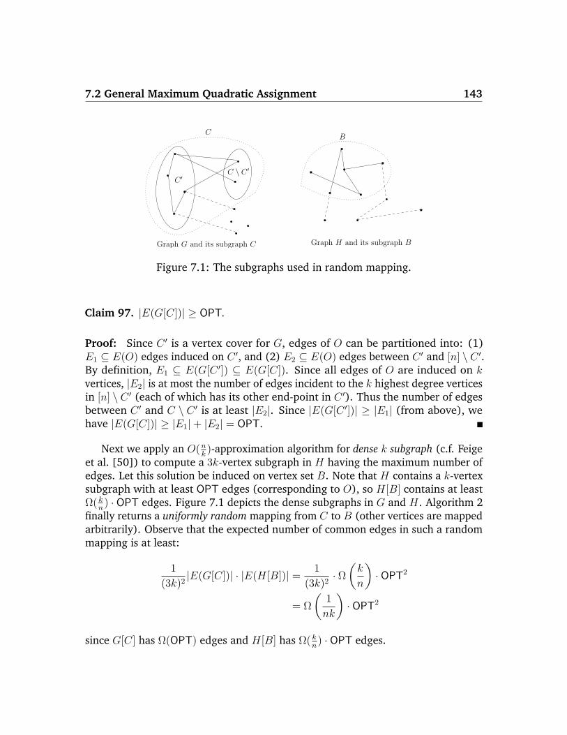
7.2 General Maximum Quadratic Assignment 143
C \ C ′
C
C ′
Graph H and its subgraph BGraph G and its subgraph C
B
Figure 7.1: The subgraphs used in random mapping.
Claim 97. |E(G[C])| ≥ OPT.
Proof: Since C ′ is a vertex cover for G, edges of O can be partitioned into: (1)E1 ⊆ E(O) edges induced on C ′, and (2) E2 ⊆ E(O) edges between C ′ and [n] \ C ′.By definition, E1 ⊆ E(G[C ′]) ⊆ E(G[C]). Since all edges of O are induced on kvertices, |E2| is at most the number of edges incident to the k highest degree verticesin [n] \ C ′ (each of which has its other end-point in C ′). Thus the number of edgesbetween C ′ and C \ C ′ is at least |E2|. Since |E(G[C ′])| ≥ |E1| (from above), wehave |E(G[C])| ≥ |E1|+ |E2| = OPT.
Next we apply an O(nk)-approximation algorithm for dense k subgraph (c.f. Feige
et al. [50]) to compute a 3k-vertex subgraph in H having the maximum number ofedges. Let this solution be induced on vertex set B. Note that H contains a k-vertexsubgraph with at least OPT edges (corresponding to O), so H[B] contains at leastΩ( k
n) · OPT edges. Figure 7.1 depicts the dense subgraphs in G and H. Algorithm 2
finally returns a uniformly random mapping from C to B (other vertices are mappedarbitrarily). Observe that the expected number of common edges in such a randommapping is at least:
1
(3k)2|E(G[C])| · |E(H[B])| = 1
(3k)2· Ω(k
n
)· OPT2
= Ω
(1
nk
)· OPT2
since G[C] has Ω(OPT) edges and H[B] has Ω( kn) · OPT edges.
144 Chapter 7: Maximum Quadratic Assignment
Combining algorithms 1 and 2. Finally we output the better of the solu-tions from Algorithms 1 and 2. The number of edges in this solution is at least
maxΩ(k),Ω( 1nk
)OPT2 ≥√
Ω(k · 1nk· OPT2) = Ω( 1√
n) · OPT. We note that the
second algorithm can be easily derandomized using conditional expectation, to givethe following.
Theorem 98. There is an O(√n) approximation for 0-1 Max-QAP. Hence there is an
O(√n log2 n) approximation algorithm for Max-QAP.
Remarks. A possible simplification to our algorithm could be just to output thebetter of maximum common star packing and a uniformly random permutation.However this algorithm achieves only an approximation ratio Ω(n2/3) as shown byan example where both graphs G and H are cliques on n2/3 vertices. We note thatthis simpler algorithm can in fact be shown to achieve a Θ(n2/3) approximationguarantee. Hence in our algorithm, it is important to find appropriate densesubgraphs before applying a random permutation.
A tight example for our algorithm is when G and H are identical√n regular
graphs that contain a perfect matching. In this case, both Algorithms 1 and 2 returnsolutions of value O(n), whereas the optimal value is ≈ n
√n.
7.2.2 Maximum Value Common Star Packing
In this section, we consider the maximum value common star packing problem:given two undirected n-vertex graphs G,H and a number 1 ≤ p ≤ n, compute amaximum value common star packing in G and H that consists of exactly p stars.We present a 5-approximation algorithm for this problem. A related problem iscapacitated star packing [8], where given a single weighted complete graph and afixed size vector s = 〈s1, · · · , sp〉, the goal is to compute a maximum weight starpacking having size vector s. Arkin et al. [8] gave a 3-approximation algorithmfor capacitated star packing. Our algorithm for common star packing is based onlocal-search and is similar to the algorithm in [8].
In Algorithm 1 for 0-1 Max-QAP, we require the maximum value common starpacking when the number of stars p is not fixed: for this purpose we run thealgorithm for fixed p (described below) over all values of 1 ≤ p ≤ n, and pick thebest common star packing.
The algorithm for common star packing always maintains a common star packinggiven by a pair of star packings S = S1, · · · , Sp in G and T = T1, · · · , Tp in H,
7.2 General Maximum Quadratic Assignment 145
where Si and Ti have the same size (for all 1 ≤ i ≤ p). For a common star packing〈S, T 〉 as above, we denote by E(S) = tpi=1E(Si) (resp. E(T ) = tpi=1E(Ti)) the setof edges in S (resp. T ). Observe that the value of this common star packing is|E(S)| = |E(T )|. We define a bijection σ : E(S) → E(T ) that maps each edge inE(Si) to some edge in E(Ti) (for every 1 ≤ i ≤ p).
Given any common star packing 〈S, T 〉, a local move is specified by a tuple〈i, xi, yi, c′i〉 where:
• Index 1 ≤ i ≤ p specifies a pair of stars Si ∈ S and Ti ∈ T .
• Vertices xi ∈ G and yi ∈ H denote new centers of the stars.
• 0 ≤ c′i ≤ n denotes the new (common) size of the stars.
Let v = |E(S)| = |E(T )| denote the value of the common star packing. Applyingmove 〈i, xi, yi, c′i〉 to 〈S, T 〉 involves the following modifications (below, two edgesare called independent if they are not incident to a common vertex).
1. Remove edges E(Si) from E(S) and E(Ti) = σ(E(Si)) from E(T ).
2. Let Xi ⊆ E(S) denote the edges of E(S) incident to vertex xi in graph G.Remove Xi from E(S) and σ(Xi) from E(T ).
3. Let Yi ⊆ E(T ) denote the edges of E(T ) incident to vertex yi in graph H.Remove Yi from E(T ) and σ−1(Yi) from E(S).
4. Let Ai denote any set of c′i edges incident to vertex xi in G such that edges inAi are independent of edges in E(S). If there does not exist such an Ai, thelocal move fails.
5. Let Bi denote any set of c′i edges incident to vertex yi in H such that edges inBi are independent of edges in E(T ). If there does not exist such a Bi, thelocal move fails.
6. Add Ai to E(S) and Bi to E(T ), and augment bijection σ so that σ(Ai) = Bi.
In steps 1-3, we only remove corresponding pairs of edges (under bijection σ)from E(S) and E(T ). This ensures that after these modifications 〈S, T 〉 remains acommon star packing. Furthermore, the value of 〈S, T 〉 after step 3 is v − |Si| −|Xi| − |Yi|. If the local move does not fail, then we obtain sets Ai and Bi in steps 4-5.
146 Chapter 7: Maximum Quadratic Assignment
Note that Ai (resp. Bi) corresponds to a c′i size star centered at xi (resp. yi) ingraph G (resp. H). By its definition, star Ai (resp. Bi) can be added to S (resp. T )to obtain a star packing. Since |Ai| = |Bi| = c′i, after step 6, 〈S, T 〉 is a commonstar packing of value v + c′i − |Si| − |Xi| − |Yi|. Finally the local move is said to beimproving iff it does not fail and the increase in value c′i − |Si| − |Xi| − |Yi| > 0.
The algorithm is initialized with S and T being zero-value star packings ingraphs G and H respectively. Then it performs any sequence of improving localmoves, until no further improvement is possible. The value of the solution increasesby at least one in each step, and the maximum value of a common star packing isn (number of vertices). So the number of iterations is at most n. The number oflocal moves at any step is at most n4, and each local move (steps 1-6) can be easilyperformed in polynomial time. Thus the entire algorithm runs in polynomial time.
We now argue that any locally optimal solution is a 5-approximate solution.Let S = S1, · · · , Sp in G and T = T1, · · · , Tp in H denote the common starpacking at a local optimum, where |Si| = |Ti| = ci for all 1 ≤ i ≤ p. Similarly letS∗ = S∗1 , · · · , S∗p in G and T ∗ = T ∗1 , · · · , T ∗p in H denote the optimal commonstar packing, where |S∗i | = |T ∗i | = c∗i for all 1 ≤ i ≤ p. For any vertex u ∈ G (resp.v ∈ H) define τ(S, u) (resp. τ(T , v)) to be the number of edges of E(S) (resp.E(T )) that are incident at u (resp. v). Also define touch(S∗i ) :=
∑u∈S∗i
τ(S, u) andtouch(T ∗i ) :=
∑v∈T ∗i
τ(T , v). Since S, S∗, T , and T ∗ are star packings,
p∑i=1
touch(S∗i ) ≤ 2
p∑i=1
ci andp∑i=1
touch(T ∗i ) ≤ 2
p∑i=1
ci (7.1)
Claim 99. For any 1 ≤ i ≤ p, we have c∗i − ci − touch(S∗i )− touch(T ∗i ) ≤ 0.
Proof: Fix a 1 ≤ i ≤ p. Suppose for a contradiction that c∗i − ci − touch(S∗i ) −touch(T ∗i ) > 0. Let xi ∈ G be the center of star S∗i and yi ∈ H the center of starT ∗i . Let αi (resp. βi) denote the number of edges in S (resp. T ) incident to xi(resp. yi). Define c′i = c∗i − touch(S∗i )− touch(T ∗i ) +αi + βi. Consider the local move〈i, xi, yi, c′i〉. Observe that when this move is applied to 〈S, T 〉, we have |Xi| = αiand |Yi| = βi in steps 2-3. Since touch(S∗i ) is the number of edges of S incidentto star S∗i and αi is the number of edges in S incident to xi, there are at least|S∗i |− (touch(S∗i )−αi) edges of star S∗i that are independent of E(S) in step 4. Sincec′i ≤ c∗i + αi − touch(S∗i ), step 4 succeeds. By an identical argument, it follows thatstep 5 also succeeds. Finally, the increase in value by this local move is:
c′i − ci − |Xi| − |Yi| = c∗i − ci − touch(S∗i )− touch(T ∗i ) > 0
7.2 General Maximum Quadratic Assignment 147
But this contradicts the fact that 〈S, T 〉 is a local optimum.
Adding the p expressions given by Claim 99 and using Equation (7.1), we have:p∑i=1
c∗i −p∑i=1
ci −p∑i=1
touch(S∗i )−p∑i=1
touch(T ∗i ) ≤ 0
=⇒p∑i=1
c∗i − 5
p∑i=1
ci ≤ 0
Hence any local optimum is a 5-approximate solution.
Theorem 100. There is a 5-approximation algorithm for maximum value commonstar packing.
7.2.3 Asymmetric Maximum Quadratic Assignment
We note that our algorithm for the general Max-QAP problem extends readily tothe case when the matrices W,D are asymmetric. The reduction to 0-1 Max-QAP(Lemma 95) clearly holds in the asymmetric case as well. Hence it suffices toconsider the directed version of 0-1 Max-QAP, where given two n-vertex directedgraphs, the goal is to find a permutation of one graph that maximizes the numberof common directed edges. Following the notation in Section 7.2.1, if k denotes thenumber of non-isolated vertices in the optimal graph O, then Claim 96 implies thatO contains a star-packing (in the undirected sense) of size at least k/4. It followsthat there is either an In-star packing (where edges of each star are directed to itscenter) or an Out-star packing (where edges of each star are directed away from itscenter) having size k/8. The Common Star Packing algorithm of Section 7.2.2 easilyextends to give a constant factor approximation for computing a maximum valuecommon In-star (resp. Out-star) packing in two directed graphs. So Algorithm 1 isguaranteed to find a solution of value Ω(k).
In Algorithm 2, we consider both graphs as being undirected. Then exactly asbefore, we obtain two 3k vertex subgraphs such that one of them has Ω(1)OPTedges and the other Ω( k
n)OPT edges. Finally observe that a uniformly random
mapping of two r-vertex directed graphs having m1 and m2 edges results in m1·m2
r2
common directed edges in expectation. So Algorithm 2 outputs a solution of valueΩ( 1
nk)OPT2. Thus we obtain the following.
Corollary 101. There is an O(√n log2 n) approximation algorithm for asymmetric
Max-QAP.
148 Chapter 7: Maximum Quadratic Assignment
7.3 Max-QAP under Triangle Inequality
In this section we treat the special case of the Maximum Quadratic AssignmentProblem where the entries of matrix D satisfy the triangle inequality, i.e. dij + djk ≥dik for all i, j, k ∈ [n]. Recall that W and D are symmetric.
Let G and H be the complete undirected graphs with edge weights defined bymatrices W and D, respectively. Let M be the matching in graph H (where weightssatisfy triangle inequality) obtained by the straightforward greedy algorithm: pickthe heaviest edge in graph H and delete all incident edges, in the remaining graphchoose the heaviest edge and so on. We will call such a matching M greedy. Notethat |M | = bn/2c since H is a complete graph. Each edge e of graph H is incidentwith either one or two edges of matching M . For any edge e ∈ H, let m(e) be theedge in M with the largest weight that is incident to e. By the construction of thegreedy matching M , we have dm(e) ≥ de for all e ∈ H.
We consider the following modification of the given Max-QAP instance, whichwe call the auxiliary problem. Find a permutation π of [n] that maximizes:∑
i,j∈[n],i 6=j
wi,j · dm(π(i),π(j)), (7.2)
i.e. the weight of each edge (i, j) in graph G is multiplied by the weight of edgem(π(i), π(j)) in graph H (which is incident to the edge (π(i), π(j)) in H). Let OPT∗
be the value of the optimal solution to the Max-QAP instance, and let Aux∗ be theoptimal value of the auxiliary problem (7.2). We first prove a simple lemma basedon triangle inequality.
Lemma 102. Aux∗ ≥ OPT∗ ≥ Aux∗/2
Proof: Since dm(e) ≥ de for all edges e ∈ H, we obtain the first inequalityAux∗ ≥ OPT∗.
Consider now an optimal solution (permutation) σ for the auxiliary problem(7.2), that maps vertices of G to those of H. Let σ′ denote the random permutationwhere we swap assignments along each edge of matching M with probability 1/2.More precisely, consider an edge (u, v) ∈M such that i and j are the two verticesof graph G mapped to the endpoints of this, i.e. u = σ(i) and v = σ(j). We setσ′(i) = u, σ′(j) = v with probability 1/2, and σ′(i) = v, σ′(j) = u with probability1/2. This process is repeated independently for all edges of the greedy matching M .
7.3 Max-QAP under Triangle Inequality 149
We now prove that the expected value of the original Max-QAP instance on therandom permutation σ′ is at least Aux∗/2 that would imply the second inequalityof the lemma. Consider an edge (i, j) in graph G, and let σ(i) = u and σ(j) = v. If(u, v) ∈M , then the expectation of the term corresponding to (i, j) in the objectivefunction of Max-QAP on permutation σ′ is exactly wijdu,v. If (u, v) 6∈ M and bothu and v are incident to edges from M , then let u and v be the other endpoints ofedges from M incident to u and v, i.e. (u, u) ∈ M and (v, v) ∈ M . In this case, bytriangle inequality the expectation of the objective function term corresponding to(i, j) on permutation σ′ is exactly:
wij(du,v + du,v + du,v + du,v)/4 ≥ wijmaxdu,u, dv,v
2= wij · dm(σ(i),σ(j))/2
Analogously, if vertex u or v (say v) is the single vertex of H that is not incidentto any edge of the greedy matching M and (u, u) ∈M , then the expectation of theobjective function term corresponding to (i, j) on permutation σ′ is:
wij(du,v + du,v)/2 ≥ wij · du,u/2 = wij · dm(σ(i),σ(j))/2.
Summing up the contribution to the Max-QAP objective over all edges (i, j) ∈ G,the expected value of permutation σ′ is at least Aux∗
2which implies OPT∗ ≥ Aux∗/2.
7.3.1 Algorithm for the auxiliary problem
In the rest of the section, we will show how to construct a (1− 1e) approximation
algorithm for the auxiliary problem. We consider the following more generalproblem. The input is an undirected edge-weighted graph G = (V,E,w) withnonnegative edge weights we ≥ 0 for e ∈ E and nonnegative numbers ∆ini=1. Thegoal is to find a permutation π of vertices of graph G that maximizes objective:
2∑
(i,j)∈E
wij ·( n∑p=minπi,πj
∆p
)(7.3)
We first reduce the auxiliary problem (7.2) to one of the above form (7.3). Theweighted graph G is the complete graph on vertex set V = [n] with edge-weights W .
150 Chapter 7: Maximum Quadratic Assignment
Let l = bn/2c and D1 ≥ D2 ≥ · · · ≥ Dl be the edge-weights of greedy matching M .We set ∆2q = Dq−Dq+1 for all 1 ≤ q ≤ l (here Dl+1 = 0), and all other ∆s are set to0. We also renumber vertices in graph H, in the auxiliary problem (7.2), so that theedges in the greedy matching M are chosen in the order (1, 2), (3, 4), · · · , (2l−1, 2l).Now for any permutation π and vertices i, j in G, we have
dm(π(i),π(j)) =n∑
p=minπ(i),π(j)
∆p
Hence objective (7.3) equals objective (7.2) for every permutation (note that (7.2)sums over unordered pairs i, j whereas (7.3) sums over ordered pairs). In thefollowing, we obtain an approximation algorithm for Problem (7.3).
Problem (7.3) generalizes the Maximum Vertex Cover problem where, given anedge-weighted undirected graph and a number k, the goal is to find k verticesthat cover the maximum weight of edges. The maximum vertex cover problem isAPX-hard [125] and the best known approximation ratio is ≈ 3
4[51]. We present a
(1− 1e) approximation algorithm for problem (7.3) using a natural LP relaxation. In
the following, x-variables are assignment variables mapping vertices to positions,and each variable zijs denotes whether either of vertices i, j ∈ V is mapped to someposition in 1, · · · , s (where s ∈ [n]).
max 2 ·∑
(i,j)∈E
wij
n∑s=1
∆szijs,
zijs ≤s∑t=1
xit +s∑t=1
xjt, ∀(i, j) ∈ E, ∀s = 1, . . . , n (7.4)
zijs ≤ 1, ∀(i, j) ∈ E, ∀s = 1, . . . , n (7.5)∑i∈V
xit = 1, ∀t = 1, . . . , n (7.6)
n∑t=1
xit = 1, ∀i ∈ V (7.7)
xit ≥ 0, ∀i ∈ V, ∀t = 1, . . . , n (7.8)zijs ≥ 0, ∀(i, j) ∈ E, ∀s = 1, . . . , n (7.9)
Our algorithm is quite a natural randomized rounding of the optimal solution(x∗, z∗) of the above linear program. For each position t = 1, . . . , n we treat con-straint (7.6) as a density function and choose a vertex i ∈ V at random according
7.3 Max-QAP under Triangle Inequality 151
to this distribution, to assign to position t. After that, each position t = 1, . . . , n hasone chosen vertex. If a vertex is chosen by many positions then we assign it to theearliest one. The vertices not chosen by any position in the previous step of thealgorithm are assigned to arbitrary empty positions.
We now derive the expected performance guarantee of the algorithm. For eachedge (i, j) ∈ E we estimate its contribution to the objective function:
wij
n∑s=1
∆s · Pr(i or j is assigned a position ≤ s)
= wij
n∑s=1
∆s ·(
1−s∏t=1
(1− x∗it − x∗jt))
(7.10)
≥ wij
n∑s=1
∆s
(1− e−
∑st=1(x∗it+x
∗jt))
(7.11)
≥ wij
n∑s=1
∆s
(1− 1
e
)·min
s∑t=1
(x∗it + x∗jt), 1
(7.12)
=
(1− 1
e
)wij
n∑s=1
∆sz∗ijs
Inequality (7.11) follows from the fact that 1 + x ≤ ex for all x ∈ R, and inequal-ity (7.12) from 1 − e−x ≥ (1 − 1
e)x for 0 ≤ x ≤ 1. Therefore, the total expected
objective function value of the rounded solution is at least 1− 1e
times the optimalvalue of the linear programming relaxation. Combined with Lemma 102, we havethe following.
Theorem 103. There is a 2ee−1
approximation algorithm for Max-QAP with triangleinequality.
Derandomization. The above randomized rounding algorithm can be derandom-ized using conditional expectations since we have an exact expression for the ex-pected objective value (7.10). Similarly, the algorithm in Lemma 102, that obtainsa solution to Max-QAP from one for problem (7.2) can be easily derandomized.Hence we obtain a deterministic algorithm in Theorem 103.
152 Chapter 7: Maximum Quadratic Assignment
7.4 Some Remarks on an LP Relaxation for Max-QAP
Consider the following integer program for Max-QAP. We have assignment variablesxi,p between vertices of the two graphs, and variables yi,p,j,q denote whether “i mapsto p and j maps to q”. The LP relaxation LP is obtained by dropping the integralitycondition on variables, and is given below.
max∑
i,j∈[n],i 6=j
wij∑
p,q∈[n],p 6=q
dpq · yi,p,j,q,
n∑i=1
xi,p = 1, ∀ 1 ≤ p ≤ n
n∑p=1
xi,p = 1, ∀ 1 ≤ i ≤ n
n∑i=1
yi,p,j,q = xj,q, ∀ 1 ≤ p, j, q ≤ n
n∑p=1
yi,p,j,q = xj,q, ∀ 1 ≤ i, j, q ≤ n
n∑j=1
yi,p,j,q = xi,p, ∀ 1 ≤ i, p, q ≤ n
n∑q=1
yi,p,j,q = xi,p, ∀ 1 ≤ i, j, p ≤ n
xi,p ≥ 0, ∀ 1 ≤ i, p ≤ nyi,p,j,q ≥ 0, ∀ 1 ≤ i, p, j, q ≤ n.
General Max-QAP. The dense k subgraph problem is the special case of Max-QAPwhen matrix D is the incidence matrix of a k-clique (i.e. dpq = 1 if 1 ≤ p, q ≤ k,and dpq = 0 otherwise), and W is the incidence matrix of the input graph. We notethat in the case of dense k subgraph, this LP can be shown to have an integralitygap of O(
√n): LP is at least as good as the standard LP for dense k subgraph,
which has integrality gap ≈ nk
(due to Goemans); in addition LP cannot have valuelarger than mink2,m (where m is number of edges in the input graph), so itsintegrality gap is at most k. The following example shows that this is nearly tight.Consider k =
√n, and a random k-regular graph (see Wormald [158] for such
models) corresponding to W . With high probability, the optimal value of the integer
7.4 Some Remarks on an LP Relaxation for Max-QAP 153
program can be bounded by O(k log n). However, the LP solution when all xi,p = 1n
can be shown to have objective value Ω(k2). This gives an Ω(√n
logn) lower bound on
the integrality gap of LP.
Triangle inequality Max-QAP. We also observe that for Max-QAP with triangleinequality, our approximation algorithm (Section 7.3) implies the same upper boundon the integrality gap for the above LP relaxation. Given an optimal solution (x, y) toLP for Max-QAP, we induce a solution (x, z) for the LP relaxation for problem (7.3),where xit = xit for all i, t ∈ [n] and zijs =
∑sp=1(
∑nq=1 yipjq +
∑nq=s+1 yiqjp) for all
1 ≤ i < j ≤ n, s ∈ [n]. One can easily check that zijs ≤ 1 and zijs ≤∑s
t=1(xit + xjt):
zijs =s∑
p=1
n∑q=1
yipjq +n∑
q=s+1
s∑p=1
yiqjp ≤n∑p=1
n∑q=1
yipjq = 1,
and,
zijs =s∑
p=1
n∑q=1
yipjq +s∑
p=1
n∑q=s+1
yiqjp
≤s∑
p=1
xip +s∑
p=1
n∑q=1
yiqjp
=s∑
p=1
(xip + xjp)
So (x, z) is indeed feasible. As for the first inequality in Lemma 102, we can arguethat the LP-objective (in problem (7.3)) of (x, z) is at least the LP-objective of (x, y)in LP . Then the LP-rounding algorithm for problem (7.3) together with the secondpart of Lemma 102 implies that the integrality gap of the above LP for Max-QAP isat most 2e
e−1, when one of the matrices satisfies triangle inequality.
Credits: The results in this chapter are from “On the Maximum Quadratic AssignmentProblem” [116], obtained jointly with Maxim Sviridenko.

Chapter 8
Conclusions
In this thesis we gave approximation algorithms for a number of sequencing prob-lems. The main focus was on vehicle routing problems. As a broader goal wealso studied two other sequencing problems: one from machine scheduling andan assignment problem. The VRPs considered here capture various aspects of ve-hicle routing, such as capacity constraints, possibility of transshipment, stochasticdemands and asymmetric distances.
We now mention some open problems and future directions from this thesis.For the single vehicle non-preemptive Dial-a-Ride problem, there is still a large gapbetween the best known O(
√minn, k) approximation and its APX-hardness. Our
approach for this Dial-a-Ride problem essentially reduces it to the k-forest problem(which is a generalization of dense-k-subgraph); a natural open question is whetherthere is a reduction in the reverse direction.
The notion of preemption is well-studied in machine scheduling problems,however this aspect has not been investigated as much in the context of VRPs. Inthis thesis we studied the preemptive multi-vehicle Dial-a-Ride problem. In manyVRPs, transshipment reduces costs by a significant amount. Modeling transhipmentin such VRPs and designing good algorithms is an interesting future direction.
There is a substantial body of work (eg. [92, 15, 16]) on a priori strategiesfor VRPs under probabilistic demands, however much less is known for adaptivestrategies. In stochastic demands VRP, we considered adaptive strategies for thebasic capacitated vehicle routing problem under demand uncertainty. It would beinteresting to study adaptive strategies for other VRPs and scheduling problems.
Most of the existing work on VRPs deal with only symmetric metrics. In asymmet-
155
156 Chapter 8: Conclusions
ric metrics, even the basic traveling salesman problem is not very well understood:the currently best-known approximation ratio is O(log n), and improving this boundis a major open question. In this thesis we studied the orienteering and minimumlatency problems on asymmetric metrics. Obtaining approximation algorithms forother VRPs under asymmetric distances is another direction for future work. Aspecific open question is the integrality gap of the LP relaxation for asymmetrictraveling salesman path that was studied in Chapter 5; we conjecture an O(log n)bound. This would imply a poly-logarithmic approximation for directed minimumlatency in quasi-polynomial time.
In the permutation flow shop scheduling problem, there is again a big gap betweenthe best-known O(
√minm,n)-approximation and its strong NP-hardness (even
with m = 3 machines [61]). This algorithm is relative to the obvious lower boundsof job-length and machine-load; and it is the best possible result using these lowerbounds [126]. Hence stronger lower bounds would be needed to obtain betterapproximation algorithms. It is interesting to note that nearly logarithmic approxi-mations are known for two related problems: usual flow shop (without permutationconstraint) [40], and no-wait permutation flow shop (with the additional constraintthat jobs can not wait between machines) [157, 150].
Both the k-forest and maximum quadratic assignment problems generalize dense-k-subgraph, which is a well-studied problem in approximation algorithms. Im-proving the best known n1/3−δ approximation guarantee [50] for dense-k-subgraph(δ > 0 is a small constant) is a challenging open question. On the other hand, thebest known hardness of approximation for dense-k-subgraph is that it does notadmit a PTAS [95].
Bibliography
[1] W. P. Adams and T. A. Johnson. Improved Linear Programming-based LowerBounds for the Quadratic Assignment Problem. In DIMACS Series in DiscreteMathematics and Theoretical Computer Science, volume 16, pages 43–77,1994.
[2] Micah Adler and Brent Heeringa. Approximating Optimal Binary DecisionTrees. In Proceedings of the 11th International Workshop on Approximation,Randomization and Combinatorial Optimization, pages 1–9, 2008.
[3] A. Ageev and M. Sviridenko. Pipage rounding: a new method of constructingalgorithms with proven performance guarantee. Journal of CombinatorialOptimization, 8:307–328, 2004.
[4] Ajit Agrawal, Philip Klein, and R. Ravi. When trees collide: an approximationalgorithm for the generalized steiner problem on networks. SIAM Journal onComputing, 24(3):440–456, 1995.
[5] K. Altinkemer and B. Gavish. Heuristics for unequal weight delivery problemswith a fixed error guarantee. Operations Research Letters, 6:149–158, 1987.
[6] K. Altinkemer and B. Gavish. Heuristics for delivery problems with constanterror guarantees. Transportation Research, 24:294–297, 1990.
[7] David L. Applegate, Robert E. Bixby, Vasek Chvatal, and William J. Cook. TheTraveling Salesman Problem: A Computational Study. Princeton UniversityPress, 2006.
[8] E. Arkin, R. Hassin, S. Rubinstein, and M. Sviridenko. Approximations forMaximum Transportation Problem with Permutable Supply Vector and otherCapacitated Star Packing Problems. Algorithmica, 39:175–187, 2004.
157
158 Bibliography
[9] E.M. Arkin, R. Hassin, and M. Sviridenko. Approximating the maximumquadratic assignment problem. Information Processing Letters, 77:13–16,2001.
[10] S. Arora, A. Frieze, and H. Kaplan. A new rounding procedure for theassignment problem with applications to dense graph arrangement problems.Mathematical Programming, 92(1):1–36, 2002.
[11] Sanjeev Arora. Polynomial-time Approximation Schemes for Euclidean TSPand other Geometric Problems. Journal of the ACM, 45(5):753–782, 1998.
[12] Brenda S. Baker. Approximation Algorithms for NP-Complete Problems onPlanar Graphs. Journal of ACM, 41:153–180, 1994.
[13] N. Bansal, A. Blum, S. Chawla, and A. Meyerson. Approximation Algorithmsfor Deadline-TSP and Vehicle Routing with Time Windows. pages 166–174,2004.
[14] D. Bertsimas, P. Chervi, and M. Peterson. Computational approaches tostochastic vehicle routing problems. Transportation Science, 29:342–352,1995.
[15] D. Bertsimas, P. Jaillet, and A.R. Odoni. A priori optimization. OperationsResearch, 38(6):1019 – 1033, 1990.
[16] Dimitris J. Bertsimas. A vehicle routing problem with stochastic demand.Operations Research, 40(3):574–585, 1992.
[17] A. Blum, S. Chawla, D. R. Karger, T. Lane, A. Meyerson, and M. Minkoff.Approximation Algorithms for Orienteering and Discounted-Reward TSP.SIAM Journal on Computing, 37(2):653–670, 2007.
[18] Avrim Blum, Prasad Chalasani, Don Coppersmith, William R. Pulleyblank,Prabhakar Raghavan, and Madhu Sudan. The minimum latency problem.In Proceedings of the 26th Annual ACM Symposium on Theory of Computing,pages 163–171, 1994.
[19] A. Bompadre, M. Dror, and J.B. Orlin. Improved bounds for vehicle routingsolutions. Discrete Optimization, 3(4):299–316, 2006.
159
[20] R.E. Burkard, E. Cela, P. Pardalos, and L.S. Pitsoulis. The quadratic as-signment problem. In Handbook of Combinatorial Optimization, D.Z. Du,P.M. Pardalos (Eds.), volume 3, pages 241–339. Kluwer Academic Publishers,1998.
[21] Costas Busch, Ryan LaFortune, and Srikanta Tirthapura. Improved sparsecovers for graphs excluding a fixed minor. In Proceedings of the 26th AnnualACM Symposium on Principles of Distributed Computing, pages 61–70, 2007.
[22] Eranda Cela. The Quadratic Assignment Problem: Theory and Algorithms.Springer, 1998.
[23] S. Chakrabarti, C. Phillips, A. Schulz, D. Shmoys, C. Stein, and J. Wein.Improved Scheduling Algorithms for Minsum Criteria. In Proceedings of the23rd International Colloquium on Automata, Languages, and Programming,pages 646–657, 1996.
[24] V. T. Chakravarthy, V. Pandit, S. Roy, P. Awasthi, and M. Mohania. DecisionTrees for Entity Identification: Approximation Algorithms and HardnessResults. In Proceedings of the ACM-SIGMOD Symposium on Principles ofDatabase Systems, 2007.
[25] I-M. Chao. A tabu search method for the truck and trailer routing problem.Computer and Operations Research, 29:469–488, 2002.
[26] Moses Charikar, Chandra Chekuri, Ashish Goel, and Sudipto Guha. Roundingvia trees: deterministic approximation algorithms for group Steiner trees andk median. In Proceedings of the 30th Annual ACM Symposium on Theory ofComputing, pages 114–123, 1998.
[27] Moses Charikar, Chandra Chekuri, To yat Cheung, Zuo Dai, Ashish Goel,Sudipto Guha, and Ming Li. Approximation algorithms for directed Steinerproblems. Journal of Algorithms, 33:73–91, 1999.
[28] Moses Charikar and Balaji Raghavachari. The Finite Capacity Dial-A-RideProblem. In Proceedings of 39th Annual Symposium on Foundations of Com-puter Science, pages 458–467, 1998.
[29] Kamalika Chaudhuri, Brighten Godfrey, Satish Rao, and Kunal Talwar. Paths,trees, and minimum latency tours. pages 36–45, 2003.
160 Bibliography
[30] Chandra Chekuri, Nitish Korula, and Martin Pal. Improved Algorithms forOrienteering and Related Problems. In Proceedings of the 19th Annual ACM-SIAM Symposium on Discrete algorithms, pages 661–670, 2008.
[31] Chandra Chekuri and Martin Pal. A recursive greedy algorithm for walksin directed graphs. In Proceedings of the 46th Annual IEEE Symposium onFoundations of Computer Science, pages 245–253, 2005.
[32] Chandra Chekuri and Martin Pal. An O(log n) Approximation Ratio forthe Asymmetric Traveling Salesman Path Problem. Theory of Computing,3:197–209, 2007.
[33] B. Chen, C. Potts, and G. Woeginger. A review of machine scheduling:complexity, algorithms and approximability. Handbook of combinatorialoptimization, 3:21–169, 1998.
[34] N. Christofides. Worst-case analysis of a new heuristic for the travellingsalesman problem. GSIA, CMU-Report 388, 1977.
[35] J. Chuzhoy, S. Guha, E. Halperin, G. Kortsarz, S. Khanna, R. Krauthgamer,and S. Naor. Asymmetric k-center is log∗n-hard to Approximate. Journal ofthe ACM, 52(4):538–551, 2005.
[36] V. Chvatal. A greedy heuristic for the set covering problem. Mathematics ofOperations Research, 4:233–235, 1979.
[37] M. Conforti and G. Cornuejols. Submodular set functions, matroids and thegreedy algorithm: tight worst-case bounds and some generalizations of theRado-Edmonds theorem. Discrete Applied Mathematics, 7:257–275, 1984.
[38] R. Conway, W. Maxwell, and L. Miller. Theory of scheduling. Addison-WesleyPublishing Co.
[39] Jean-Francois Cordeau and Gilbert Laporte. The Dial-a-Ride Problem (DARP):Variants, modeling issues and algorithms. 4OR: A Quarterly Journal ofOperations Research, 1(2), 2003.
[40] A. Czumaj and C. Scheideler. A New Algorithmic Approach to the GeneralLovasz Local Lemma with Applications to Scheduling and Satisfiability Prob-lems. In Proceedings of the 32nd Annual Symposium on Theory of Computing.
161
[41] Willem E. de Paepe, Jan Karel Lenstra, Jiri Sgall, Ren A. Sitters, and LeenStougie. Computer-Aided Complexity Classification of Dial-a-Ride Problems .Informs Journal on Computing, 16(2):120–132, 2004.
[42] M. Dror, G. Laporte, and P. Trudeau. Vehicle routing with stochastic demands:properties and solution frameworks. Transportation Science, 23:166176,1989.
[43] Moshe Dror. Vehicle Routing with Stochastic Demands: Models & Computa-tional Methods. In Modeling Uncertainty: International Series In OperationsResearch & Management Science, volume 46(8), pages 625–649. Springer.
[44] G. Even, N. Garg, J. Konemann, R. Ravi, and A. Sinha. Covering GraphsUsing Trees and Stars. Operations Research Letters, 32(4):309–315.
[45] Jittat Fakcharoenphol, Chris Harrelson, and Satish Rao. The k-travelingrepairmen problem. ACM Transactions on Algorithms, 3(4), 2007.
[46] Jittat Fakcharoenphol, Satish Rao, and Kunal Talwar. A tight bound onapproximating arbitrary metrics by tree metrics. Journal of Computer andSystem Sciences, 69(3):485–497, 2004.
[47] U. Feige and J.R. Lee. An improved approximation ratio for the minimumlinear arrangement problem. Information Processing Letters, 101(1):26–29,2007.
[48] U. Feige and C. Scheideler. Improved bounds for acyclic job shop scheduling.In Proceedings of the 30th Annual Symposium on Theory of Computing.
[49] Uriel Feige. A threshold of lnn for set cover. Journal of the ACM, 45:634–652,1998.
[50] Uriel Feige, Guy Kortsarz, and David Peleg. The Dense k-Subgraph Problem.Algorithmica, 29(3):410–421, 2001.
[51] Uriel Feige and Michael Langberg. Approximation Algorithms for Max-imization Problems Arising in Graph Partitioning. Journal of Algorithms,41(2):174–211, 2001.
[52] Uriel Feige, David Peleg, and Guy Kortsarz. The Dense k -Subgraph Problem.Algorithmica, 29(3):410–421, 2001.
162 Bibliography
[53] Uriel Feige and Mohit Singh. Improved Approximation Ratios for TravelingSalesperson Tours and Paths in Directed Graphs. In Proceedings of the 10thInternational Workshop on Approximation, Randomization and CombinatorialOptimization, pages 104–118, 2007.
[54] T. Feo and M. Khellaf. A class of bounded approximation algorithms forgraph partitioning . Networks, 20:181–195, 1990.
[55] A. Fishkin, K. Jansen, and M. Mastrolilli. On minimizing average weightedcompletion time: a PTAS for the job shop problem with release dates. In Pro-ceedings of the 14th International Symposium on Algorithms and Computation,pages 319–328, 2003.
[56] J. Framinan, J. Gupta, and R. Leisten. A review and classification of heuristicsfor permutation flow-shop scheduling with makespan objective. Journal ofthe Operational Research Society, 55:1243–1255, 2004.
[57] A. Frank. On Connectivity properties of Eulerian digraphs. Annals of DiscreteMathematics, 41, 1989.
[58] Greg N. Frederickson, Matthew S. Hecht, and Chul E. Kim. Approximationalgorithms for some routing problems. SIAM Journal on Computing, 7(2):178–193, 1978.
[59] A. Frieze. On the length of the longest monotone subsequence of a randompermutation . The Annals of Applied Probability, 1(2):301–305, 1991.
[60] A. Frieze, G. Galbiati, and F. Maffioli. On the worst-case performance ofsome algorithms for the asymmetric travelling salesman problem. Networks,12:23–39, 1982.
[61] M. Garey, D. Johnson, and R. Sethi. The Complexity of Flowshop andJobshop Scheduling. Mathematics of Operations Research, 1:117–129, 1976.
[62] N. Garg, G. Kojevod, and R. Ravi. A Polylogarithmic Approximation Algo-rithm for the Group Steiner Tree Problem. Journal of Algorithms, 37(1):66–84, 2000.
[63] Naveen Garg. A 3-Approximation for the Minimum Tree Spanning k Vertices.In Proceedings of the 37th Annual IEEE Symposium on Foundations of ComputerScience, pages 302–309, 1996.
163
[64] Naveen Garg. Saving an epsilon: a 2-approximation for the k-MST problemin graphs. In Proceedings of the 37th annual ACM Symposium on Theory ofcomputing, pages 396–402, 2005.
[65] Naveen Garg, Anupam Gupta, Stefano Leonardi, and Piotr Sankowski.Stochastic analyses for online combinatorial optimization problems. InProceedings of the 19th Annual ACM-SIAM Symposium on Discrete algorithms,pages 942–951, 2008.
[66] Inge Li Gørtz. Topics in Algorithms: Data Structures on Trees and Approx-imation Algorithms on Graphs. Ph.D. Thesis, IT University of Copenhagen,2005.
[67] Inge Li Gørtz. Hardness of Preemptive Finite Capacity Dial-a-Ride. In Pro-ceedings of the 9th International Workshop on Approximation, Randomizationand Combinatorial Optimization, pages 200–211, 2006.
[68] Michel X. Goemans and Dimitris J. Bertsimas. Survivable networks, linearprogramming relaxations and the parsimonious property. MathematicalProgramming, 60:145–166, 1993.
[69] Michel X. Goemans and David P. Williamson. A general approximationtechnique for constrained forest problems. SIAM Journal on Computing,24(2):296–317, 1995.
[70] Anupam Gupta. Steiner points in tree metrics don’t (really) help. In Proceed-ings of the 12th Annual ACM-SIAM Symposium on Discrete algorithms, pages220–227, 2001.
[71] Anupam Gupta, MohammadTaghi Hajiaghayi, Viswanath Nagarajan, andR Ravi. Dial a Ride from k-forest. To Appear: ACM Transactions on Algorithms(Preliminary version in European Syposium on Algorithms, 2007).
[72] N. Guttmann-Beck and R. Hassin. Approximation algorithms for min-sump-clustering. Discrete Applied Mathematics, 89:125–142, 1998.
[73] N. Guttmann-Beck and R. Hassin. Approximation algorithms for minimumtree tree partition. Discrete Applied Mathematics, 87:117–137, 1998.
[74] M. Haimovich and A. H. G. Rinnooy Kan. Bounds and heuristics for capac-itated routing problems. Mathematics of Operations Research, 10:527–542,1985.
164 Bibliography
[75] Mohammad Taghi Hajiaghayi and Kamal Jain. The prize-collecting gener-alized steiner tree problem via a new approach of primal-dual schema. InProceedings of the 17th Annual ACM-SIAM Symposium on Discrete algorithm,pages 631–640, 2006.
[76] L.A. Hall, A.S. Schulz, D.B. Shmoys, and J. Wein. Scheduling to MinimizeAverage Completion Time: Off–Line and On–Line Approximation Algorithms.Mathematics of Operations Research, 22:513–544, 1997.
[77] L.A. Hall, D.B. Shmoys, and J. Wein. Scheduling to Minimize AverageCompletion Time: Off–line and On–line Algorithms. In Proceedings of the 7thannual ACM-SIAM Symposium on Discrete Algorithms, pages 142–151, 1996.
[78] Eran Halperin and Robert Krauthgamer. Polylogarithmic inapproximability.In Proceedings of the 35th Annual Symposium on Theory of Computing, pages585–594, 2003.
[79] R. Hassin, A. Levin, and M. Sviridenko. Approximating the minimumquadratic assignment problems. Manuscript, 2008.
[80] R. Hassin and S. Rubinstein. Approximation algorithms for maximum lineararrangement. Information Processing Letters, 80:171–177, 2001.
[81] R. Hassin and S. Rubinstein. Robust matchings. SIAM Journal of DiscreteMathematics, 15:530–537, 2002.
[82] R. Hassin and S. Rubinstein. An improved approximation algorithm for themetric maximum clustering problem with given cluster sizes. InformationProcessing Letters, 98:92–95, 2006.
[83] R. Hassin, S. Rubinstein, and A. Tamir. Approximation Algorithms forMaximum Dispersion. Operations Research Letters, 21:133–137, 1997.
[84] J. Hastad. Clique is hard to approximate within n1−ε. Acta Mathematica,182:105–142, 1999.
[85] M. Held and R.M. Karp. The travelling salesman problem and minimumspanning trees. Operations Research, 18:1138–1162, 1970.
[86] D. Hochbaum and W. Maass. Approximation Schemes for Covering andPacking Problems in Image Processing and VLSI. Journal of ACM, 32:130–136, 1985.
165
[87] D.S. Hochbaum and D.B. Shmoys. A unified approach to approximationalgorithms for bottleneck problems. Journal of the ACM, 33:533–550, 1986.
[88] D.S. Hochbaum and D.B. Shmoys. Using dual approximation algorithms forscheduling problems: theoretical and practical results. Journal of the ACM,34:144–162, 1987.
[89] W.L. Hsu and G.L. Nemhauser. Easy and hard bottleneck location problems.Discrete Applied Mathematics, 1:209–216, 1979.
[90] O.H. Ibarra and C.E. Kim. Fast approximation algorithms for the knapsackand subset sum problems. Journal of the ACM, 22:463–468, 1976.
[91] B. Jackson. Some remarks on arc-connectivity, vertex splitting, and orienta-tion in digraphs. Journal of Graph Theory, 12(3):429–436, 1988.
[92] Patrick Jaillet. A priori solution of a travelling salesman problem in which arandom subset of the customers are visited. Operations Research, 36(6):929 –936, 1988.
[93] D.S. Johnson. Approximation algorithms for combinatorial optimizationproblems. Journal of Computer and System Sciences, 9:256–278, 1974.
[94] R.M. Karp. A characterization of the minimum cycle mean in a digraph.Discrete Mathematics, 23(3):309–311, 1978.
[95] Subhash Khot. Ruling out ptas for graph min-bisection, densest subgraphand bipartite clique. In Proceedings of the 45th Annual IEEE Symposium onFoundations of Computer Science, pages 136–145, 2004.
[96] S. Khuller, A. Moss, and J. Naor. The budgeted maximum coverage problem.Information Processing Letters, 70:39–45, 1999.
[97] Samir Khuller, Balaji Raghavachari, and Neal Young. Balancing minimumspanning and shortest path trees. In Proceedings of the 4th Annual ACM-SIAMSymposium on Discrete algorithms, pages 243–250, 1993.
[98] K.Jansen, R.Solis-Oba, and M. Sviridenko. Makespan Minimization in JobShops: a Linear Time Approximation Scheme. SIAM Journal of DiscreteMathematics, 16:288–300, 2003.
166 Bibliography
[99] Philip Klein, Serge A. Plotkin, and Satish Rao. Excluded minors, networkdecomposition, and multicommodity flow. In Proceedings of the 25th AnnualACM Symposium on Theory of Computing, pages 682–690, 1993.
[100] Jon Kleinberg and David Williamson. Unpublished note. 1998.
[101] S. Rao Kosaraju, Teresa M. Przytycka, and Ryan S. Borgstrom. On an OptimalSplit Tree Problem. In Proceedings of the 6th International Workshop onAlgorithms and Data Structures, pages 157–168, 1999.
[102] S. Krumke, J. Rambau, and S. Weider. An approximation algorithm for thenonpreemptive capacitated dial-a-ride problem. Preprint 00-53, Konrad-Zuse-Zentrum fr Informationstechnik Berlin, 2000.
[103] Fumei Lam and Alantha Newman. Traveling salesman path problems. Math-ematical Programming, 113(1):39–59, 2008.
[104] E.L. Lawler, J.K. Lenstra, A.H.G. Rinnooy Kan, and D.B. Shmoys. Sequencingand scheduling: Algorithms and complexity. In Handbook in OperationsResearch and Management Science, volume 4, pages 445–522. North-Holland,1993.
[105] F. Lazebnik, V.A. Ustimenko, and A.J. Woldar. A New Series of Dense Graphsof High Girth. Bulletin of the AMS, 32(1):73–79, 1995.
[106] B.F. Logan and L.A. Shepp. A Variational Problem for Random YoungTableaux. Advances in Mathematics, 26:206–222, 1977.
[107] E.M. Loilola, N.M.M. De Abreu, P.O. Boaventura-Netto, P.M. Hahn, andT. Querido. A survey for the quadratic assignment problem (Invited Review).European Journal of Operational Research, 176:657–690, 2006.
[108] L. Lovasz. On the ratio of optimal integral and fractional covers. DiscreteMathematics, 13:383–390, 1975.
[109] W. Mader. Construction of all n-fold edge-connected digraphs (German).European Journal of Combinatorics, 3:63–67, 1982.
[110] J.S.B. Mitchell. Guillotine Subdivisions Approximate Polygonal Subdivisions:Part II – A simple polynomial-time approximation scheme for geometric TSP,k-MST, and related problems. SIAM Journal on Computing, 28(4):1298–1309,1999.
167
[111] S. Mitrovic-Minic and G. Laporte. The Pickup and Delivery Problem withTime Windows and Transshipment. Information Systems and OperationalResearch, 44:217–227, 2006.
[112] C. Mues and S. Pickl. Transshipment and time windows in vehicle routing.In Proceedings of the 8th International Symposium on Parallel Architectures,Algorithms and Networks, pages 113–119, 2005.
[113] Viswanath Nagarajan and R. Ravi. Poly-logarithmic approximation algorithmsfor directed vehicle routing problems. In Proceedings of the 10th InternationalWorkshop on Approximation, Randomization and Combinatorial Optimization,pages 257–270, 2007.
[114] Viswanath Nagarajan and R. Ravi. The Directed Minimum Latency Prob-lem. In Proceedings of the 11th International Workshop on Approximation,Randomization and Combinatorial Optimization, pages 193–206, 2008.
[115] Viswanath Nagarajan and Maxim Sviridenko. Tight Bounds for Permuta-tion Flowshop Scheduling. To Appear: Mathematics of Operations Research(Preliminary version in Integer Programming and Combinatorial Optimization,2008).
[116] Viswanath Nagarajan and Maxim Sviridenko. On the Maximum QuadraticAssignment Problem. In Proceedings of the 20th Annual ACM-SIAM Symposiumon Discrete algorithms, pages 516–524, 2009.
[117] Y. Nakao and H. Nagamochi. Worst case analysis for pickup and deliveryproblems with transfer. IEICE Transactions on Fundamentals of Electronics,Communications and Computer Sciences, E91-A(9), 2008.
[118] M. Nawaz, E. Enscore Jr., and I. Ham. A heuristic algorithm for the m-machine n-job flow-shop sequencing problem. OMEGA International J. Man-agement Science, 11:91–95, 1983.
[119] George L. Nemhauser and Laurence A. Wolsey. Integer and CombinatorialOptimization. Wiley Interscience Publication, USA, 1999.
[120] G.L. Nemhauser and L. Wolsey. Maximizing submodular set functions:formulations and analysis of algorithms. In Studies of Graph and DiscreteProgramming, pages 279–301, 1981.
168 Bibliography
[121] E. Nowicki and C. Smutnicki. Worst-case analysis of an approximationalgorithm for flow-shop scheduling. Operations Research Letters, 8:171–177,1989.
[122] E. Nowicki and C. Smutnicki. New results in the worst-case analysis forflow-shop scheduling. Discrete Applied Mathematics, 46:21–41, 1993.
[123] R. Panigrahy and S. Vishwanathan. An O(log∗ n)-approximation for theasymmetric p-center problem. Journal of Algorithms, 27:259–268, 1998.
[124] P. Pardalos and eds. H. Wolkowitz. Proceedings of the DIMACS Workshop onQuadratic Assignment Problems, volume 16. 1994.
[125] E. Petrank. The hardness of approximation: gap location. ComputationalComplexity, 4:133–157, 1994.
[126] C. Potts, D. Shmoys, and D. Williamson. Permutation vs. nonpermutationflow shop schedules. Operations Research Letters, 10:281–284, 1991.
[127] M. Queyranne. Performance ratio of polynomial heuristics for triangleinequality quadratic assignment problems. Operations Research Letters, 4:231–234, 1986.
[128] M. Queyranne. Structure of a simple scheduling polyhedron. MathematicalProgramming A, 2:263–285, 1993.
[129] M. Queyranne and M. Sviridenko. Approximation Algorithms for ShopScheduling Problems with Minsum Objective. Journal of Scheduling, 5:287–305, 2002.
[130] P. Raghavan. Probabilistic construction of deterministic algorithms: approxi-mating packing integer programs. Journal of Computer and System Sciences,37:130–143, 1988.
[131] G. Reinelt. The Traveling Salesman: Computational Solutions for TSP Applica-tions. Springer, 1994.
[132] G. Robins and A. Zelikovsky. Tighter Bounds for Graph Steiner Tree Approxi-mation. SIAM Journal on Discrete Mathematics, 19:122–134, 2005.
[133] H. Rock and G. Schmidt. Machine aggregation heuristics in shop-scheduling.Methods of Operations Research, 45:303–314, 1983.
169
[134] S. Sahni and T. Gonzalez. P-complete approximation problems. Journal ofthe ACM, 23:555–565, 1976.
[135] M.W.P. Savelsbergh and M. Sol. The general pickup and delivery problem.Transportation Science, 29:17–29, 1995.
[136] F. Schalekamp and D. Shmoys. Algorithms for the universal and a priori TSP.Operations Research Letters, 36(1):1–3, 2008.
[137] Stephan Scheuerer. A tabu search heuristic for the truck and trailer routingproblem. Computer and Operations Research, 33:894–909, 2006.
[138] A. Schrijver. Combinatorial optimization: Polyhedra and efficiency. Springer-Verlag, 2003.
[139] Nicola Secomandi and Francois Margot. Reoptimization Approaches for theVehicle Routing Problem with Stochastic Demands. To appear: OperationsResearch.
[140] Danny Segev and Gil Segev. Approximate k-Steiner Forests via the LagrangianRelaxation Technique with Internal Preprocessing. In Proceedings of the 14thAnnual European Symposium on Algorithms, pages 600–611, 2006.
[141] S. Sevast’janov. On some geometric methods in scheduling theory: a survey.Discrete Applied Mathematics, 55:59–82, 1994.
[142] D. Shmoys, C. Stein, and J. Wein. Improved Approximation Algorithms forShop Scheduling Problems . SIAM Journal on Computing, 23(3):617–632,1994.
[143] David Shmoys and Kunal Talwar. A Constant Approximation Algorithm for thea priori Traveling Salesman Problem. In Proceedings of the 13th InternationalConference on Integer Programming and Combinatorial Optimization, pages331–343, 2008.
[144] C. Smutnicki. Some results of the worst-case analysis for flow shop schedul-ing. European Journal of Operational Research, 109:66–87, 1998.
[145] D. Sotelo and M. Poggi de Aragao. An Approximation Algorithm for thePermutation Flow Shop Scheduling Problem via Erdos-Szekeres TheoremExtensions . Manuscript, 2008.
170 Bibliography
[146] J. Michael Steele. Variations on the monotone subsequence theme of Erdosand Szekeres. In Discrete probability and algorithms, volume 72 of IMA Vol.Math. Appl., pages 111–131. Springer, 1995.
[147] W. Stewart and B. Golden. Stochastic Vehicle Routing: a comprehensiveapproach. European Journal of Operational Research, 14:371–385, 1983.
[148] M. Sviridenko. A Note on Permutation Flow Shop Problem. Annals ofOperations Research, 129:247–252, 2004.
[149] M. Sviridenko. A note on maximizing a submodular set function subject toknapsack constraint. Operations Research Letters, 32:41–33, 2004.
[150] Maxim Sviridenko. Makespan Minimization in No-Wait Flow Shops: APolynomial Time Approximation Scheme. SIAM J. Discret. Math., 16(2):313–322, 2003.
[151] Paolo Toth and Daniele Vigo, editors. The vehicle routing problem. Society forIndustrial and Applied Mathematics, 2001.
[152] J. H. van Lint and R. M. Wilson. A Course in Combinatorics. CambridgeUniversity Press, 1992.
[153] Vijay V. Vazirani. Approximation Algorithms. Springer, 2002.
[154] Santosh Vempala and Mihalis Yannakakis. A convex relaxation for theasymmetric tsp. In Proceedings of the 10th annual ACM-SIAM Symposium onDiscrete Algorithms, pages 975–976, 1999.
[155] A.M. Vershik and S.V. Kerov. Asymptotics of the Plancherel measure of thesymmetric group and the limit form of Young tableaux. Dokl. Akad. NaukSSSR, 233:1024–1027, 1977.
[156] David Williamson. Analysis of the held-karp heuristic for the travelingsalesman problem. Master’s thesis, MIT Computer Science, 1990.
[157] D.A. Wismer. Solution of the flowshop sheduling problem with no intermedi-ate queues. Operations Research, 20:689–697, 1972.
[158] N.C. Wormald. Models of random regular graphs. In Surveys in Combinatorics(J.D. Lamb and D.A. Preece, eds), volume 276, pages 239–298. LondonMathematical Society Lecture Note Series, 1999.