Siqueira et al. Algorithms Mol Biol (2021) 16:21 https://doi.org/10.1186/s13015-021-00200-w

RESEARCH

Approximation algorithm for rearrangement distances considering repeated genes and intergenic regionsGabriel Siqueira* , Alexsandro Oliveira Alexandrino , Andre Rodrigues Oliveira and Zanoni Dias

Abstract

The rearrangement distance is a method to compare genomes of different species. Such distance is the number of rearrangement events necessary to transform one genome into another. Two commonly studied events are the transposition, which exchanges two consecutive blocks of the genome, and the reversal, which reverts a block of the genome. When dealing with such problems, seminal works represented genomes as sequences of genes without repetition. More realistic models started to consider gene repetition or the presence of intergenic regions, sequences of nucleotides between genes and in the extremities of the genome. This work explores the transposition and reversal events applied in a genome representation considering both gene repetition and intergenic regions. We define two problems called Minimum Common Intergenic String Partition and Reverse Minimum Common Intergenic String Partition. Using a relation with these two problems, we show a �(k)-approximation for the Intergenic Transposition Distance, the Intergenic Reversal Distance, and the Intergenic Reversal and Transposition Distance problems, where k is the maximum number of copies of a gene in the genomes. Our practical experiments on simulated genomes show that the use of partitions improves the estimates for the distances.

Keywords: Genome rearrangement, Intergenic regions, Reversal

© The Author(s) 2021. Open Access This article is licensed under a Creative Commons Attribution 4.0 International License, which permits use, sharing, adaptation, distribution and reproduction in any medium or format, as long as you give appropriate credit to the original author(s) and the source, provide a link to the Creative Commons licence, and indicate if changes were made. The images or other third party material in this article are included in the article’s Creative Commons licence, unless indicated otherwise in a credit line to the material. If material is not included in the article’s Creative Commons licence and your intended use is not permitted by statutory regulation or exceeds the permitted use, you will need to obtain permission directly from the copyright holder. To view a copy of this licence, visit http:// creat iveco mmons. org/ licen ses/ by/4. 0/. The Creative Commons Public Domain Dedication waiver (http:// creat iveco mmons. org/ publi cdoma in/ zero/1. 0/) applies to the data made available in this article, unless otherwise stated in a credit line to the data.

IntroductionIn the field of Computational Biology, when analyzing the relationship between two genomes, one can estimate the evolutionary distance by calculating the number of muta-tions necessary to transform one genome into another. These mutations can be non-conservative (i.e., affect the quantity of genetic material), which is the case of inser-tion, deletion, duplication, or substitution of individual nucleotides [1–3], or the mutations can be conservative (i.e., do not insert or remove genetic material), which is the case of the conservative genome rearrangement events [4], which affect only the order and orientation of genes in the genome.

Some conservative events affect a single chromosome, such as the reversal, which inverts a sequence of genes, and the transposition, which exchanges the position of two consecutive sequences of genes. There are also events that may affect more than one chromosome, such as translocation, which swaps extremities of two chro-mosomes. The translocation and reversal events can be simulated by the Double-Cut-and-Join (DCJ) [5] opera-tion, which cuts the genome at two positions and cre-ates two new adjacencies by joining the four extremities affected by these cuts. This work focuses on the reversal and transposition events, consequently, we only consider genomes with a single chromosome.

When comparing genomes with a rearrangement-based distance, one must select a rearrangement model (i.e., the set of allowed rearrangement events) and find a representation for the genomes suitable to the selected

Open Access

Algorithms forMolecular Biology

*Correspondence: gabriel.siqueira@ic.unicamp.brInstitute of Computing, University of Campinas, Campinas, Brazil

Page 2 of 23Siqueira et al. Algorithms Mol Biol (2021) 16:21

model. With a given model, a rearrangement distance problem aims at finding the minimum number of allowed rearrangement events necessary to transform one genome into another.

Genomes can be represented by a string, where each character represents a gene. There may be multiple genes represented by the same characters, those genes consti-tute a gene family.

If we assume that there are no replicated characters, the characters are usually represented by integer num-bers, and a string of size n corresponds to a permutation of numbers from 1 to n. In this case, when comparing two genomes G and H of size n, one of them is repre-sented by the identity permutation ι = (1 2 . . . n) and the other by a permutation π . Consequently, finding the rearrangement distance is equivalent to finding the mini-mum number of allowed rearrangement events necessary to sort the permutation π.

A string (or a permutation) may also include informa-tion regarding gene orientation, and such information is encoded as signs, + or −, associated with each char-acter. In this case, we have a signed string (or a signed permutation).

When there are replicated characters, two common approaches are adopted to transform the strings into permutations. The first selects an exemplar of each gene family [6], and the second establishes a correspondence between characters of both strings [7, 8], which allows us to discriminate between multiple copies of the same character. The second approach has the advantage of los-ing less information but can only be applied when such correspondence can be established. In the presence of non-conservative events, the correspondence between genes may not be possible, and a preprocessing step is required to eliminate genes present in only one of the genomes.

In biological terms, this correspondence is called an orthologous assignment. The distance between permuta-tions resulting from an orthologous assignment gives us a valid upper bound for the distance between the original strings. As there are multiple possible assignments, there are some strategies to find assignments that lead to lower distances [7, 8].

Recent works [9, 10] argue that considering the size of intergenic regions (i.e., number of nucleotides between genes and in the extremities of the genome) improves the estimated distances. When the sizes of intergenic regions are taken into account, the genome representa-tion includes a string representing the gene sequence and a sequence of integers corresponding to the size of each intergenic region.

Each combination of genome representation and rear-rangement model defines a different rearrangement

distance problem. Table  1 shows a summary of results from the literature, considering different rearrangement distance problems and the contributions of the present work (last three rows). For each problem, we mention whether there is a known polynomial-time algorithm or an NP-hardness proof and, in the last case, what is the best known approximation factor for that problem.

It is worth mentioning that, to ensure an approxima-tion, the distance between strings takes into account the result of the string partition problems [26]. Such prob-lems seek to split two strings into sub-strings that can be concatenated in different orders to form the original strings. The way in which the sub-strings appear in each original string defines the problem. If the sub-strings must appear in the same orientation in both original strings, we have the minimum common string par-tition problem. If the sub-strings can appear inverted in the original strings, we have the signed minimum common string partition problem when consider-ing signed strings, and the reverse minimum common string partition problem when considering unsigned strings.

If there is an ℓ-approximation for the minimum com-mon string partition problem, then there exists a 3ℓ-approximation for the transposition distance on strings problem [21]. Similarly, if there is an ℓ-approxi-mation for the signed minimum common string par-tition problem, then there exists a 2ℓ-approximation for the reversal distance on signed strings problem [7]. The same relation can be applied to the reversal distance on strings and the reverse minimum com-mon string partition problems [26].

The best known approximation algorithms for the par-tition problems have factors in O(log n log∗ n) [27], where n is the size of the string, and in �(k) [20], where k is the maximum number of copies of a character in the string.

This work describes approximation algorithms for the intergenic transposition distance, intergenic reversal distance, and intergenic reversal and transposition distance problems, where the rep-resentation of the genomes takes into account both repeated genes and intergenic regions. Initially, we pre-sent some definitions and formalize the problems. Next, we generalize the minimum common string parti-tion and the reverse minimum common string par-tition problems to consider intergenic regions. We also present relations between the partitions and distance problems that consider intergenic regions and describe a �(k)-approximation algorithm for the partition prob-lems ensuring a �(k)-approximation for the distance problems. Finally, we performed some practical tests on simulated genomes to evaluate the improvement in

Page 3 of 23Siqueira et al. Algorithms Mol Biol (2021) 16:21

the estimates for the distances caused by the partition algorithms.

DefinitionsIn the following definitions we use ordered sequences of elements (lists). The number of elements in a list X is denoted by |X|, and an element at the i-th position of a list X is denoted by Xi . The list Y = rev(X) is equal to the list X in the reverse order (i.e., |X | = |Y | and Yi = X|X |−i+1, ∀1 ≤ i ≤ |X | ). A list of characters is called a string.

Given a string S, the set �S of distinct elements of S is the alphabet of S and each element of �S is called label. The occurrence of a label α in a string S is the num-ber of characters of S with label α , and is denoted by occ(α, S) . The maximum occurrence of any character in S is occ(S) = maxα∈�S (occ(α, S)) . A character whose label has occurrence one is called a singleton, and a character whose label has occurrence at least two is called a rep-lica. Two strings S and P are balanced if �S = �P and

occ(α, S) = occ(α,P),∀α ∈ �S . In other words, balanced strings are formed by the same characters in possibly dif-ferent orders.

When modeling genomes, we consider the intergenic regions between genes represented by their sizes. Usually, an actual genome starts and ends with intergenic regions but, to construct our representation, we include two arti-ficial genes in the beginning and end of the genome. In this process, usually called extension or capping, we use the same pair of genes for any genome.

Formally, a genome G = (g1, g1, g2, . . . , gn−1, gn) with size n is an interleaved sequence of n genes ( g1, . . . , gn ) and n− 1 intergenic regions ( g1, . . . , gn−1 ). We represent a genome G = (S, S) with a string S and a list of integers S , such that:

• The gene gi is represented by the character Si of S, for 1 ≤ i ≤ n.

• The intergenic region gi is represented by the integer Si of S , for 1 ≤ i ≤ n− 1.

Table 1 Summary of results for rearrangement problems

aSome approximations depend on k, which is the maximum number of copies of a character in the string.bAsymptotic approximation

Problem Rearrangement model Genome representation Complexity Best known approximation factor

Sorting Permutations by Transpositions Transpositions Permutation NP-hard [11] 1.375 [12]

Sorting Permutations by Reversals Reversals Permutation NP-hard [13] 1.375 [14]

Sorting Signed Permutations by Reversals Reversals Signed permutation P [15] –

Sorting Permutations by Reversals and Transpositions

Reversals and transpositions Permutation NP-hard [16] 2.8334+ ǫ [17, 18]

Sorting Signed Permutations by Reversals and Transpositions

Reversals and transpositions Signed permutation NP-hard [16] 2 [19]

Transposition Distance on Strings Transpositions String NP-hard 12ka [20, 21]

Reversal Distance on Strings Reversals String NP-hard 16ka [20]

Signed Reversal Distance on Strings Reversals Signed string NP-hard [22] 16ka [7, 20]

Sorting Permutations by Intergenic Transpositions

Transpositions Permutation and sequence of integers NP-hard [23] 3.5 [23]

Sorting Permutations by Intergenic Reversals

Reversals Permutation and sequence of integers NP-hard [24] 4 [24]

Sorting Signed Permutations by Inter-genic Reversals

Reversals Signed permutation and sequence of integers

NP-hard [16] 2 [16]

Sorting Permutations by Intergenic Rever-sals and Transpositions

Reversals and transpositions Permutation and sequence of integers NP-hard [24] 4.5 [24]

Sorting Signed Permutations by Inter-genic Reversals and Transpositions

Reversals and transpositions Signed permutation and sequence of integers

NP-hard [25] 3 [25]

Intergenic Reversal Distance on Strings Reversals String and sequence of integers NP-hard(Theorem 1)

6ka,b (Corollary 2)

Intergenic Transposition Distance on Strings

Transposition String and sequence of integers NP-hard(Theorem 1)

8ka (Corollary 4)

Intergenic Reversal and Transposition Distance on Strings

Reversal and transposition String and sequence of integers NP-hard(Theorem 1)

9ka (Corollary 5)

Page 4 of 23Siqueira et al. Algorithms Mol Biol (2021) 16:21

Two genomes G = (S, S) and H = (P, P) are called co-tailed if they have the same initial and final gene (i.e., S1 = P1 and Sn = Pn ). Note that, any two genomes result-ing from an extension are co-tailed.

The reverse of a genome G = (S, S) , denoted by rev(G) , is a genome represented by the lists rev(S) and rev(S) . We say that two genomes G and H are equal ( G = H ) if their correspondent strings and their correspondent integer lists are equal. Additionally, we say that two genomes G and H are congruent ( G ∼= H ) if G = H or G = rev(H) . Figure 1 shows an example of a genome and its reverse.

Given a genome G = (S, S) , the subgenome Gi,j = (Si,j , Si,j) is the portion of genome G between the genes gi and gj . Consequently, the subgenome Gi,j is rep-resented by lists Si,j and Si,j , such that:

A genome G contains another genome H if H is equal to some subgenome of G . We denote that relation by H ⊂ G . We also use H ⊂ G to indicate that G does not contain H.

Let us define an operation of a combination of genomes (exemplified in Fig. 2). We say that a genome K = (Q, Q) is a combination of two genomes G = (S, S) and H = (P, P) if:

Si,jk = Si+k−1, ∀1 � k � j − 1+ 1

Si,jk = Si+k−1, ∀1 � k � j − 1

• Q is the concatenation of the strings S and P.• Q is formed by the list S followed by an integer (rep-

resenting the size of the intergenic region between the two genomes) and then followed by the list P.

Two genomes G = (S, S) and H = (P, P) of size n are balanced if:

• The strings S and P are balanced.• The sum of the integers correspondent to intergenic

regions are the same, i.e., ∑n

i=1 Si =∑n

i=1 Pi

Given two balanced genomes G = (S, S) and H = (P, P) , an orthologous assignment ξ between them is a mapping between genes, i.e., for each gene Si of S there is a cor-respondent gene ξ(Si) in P. We denote the intergenic region after the gene ξ(Si) by ξ(Si) . Each singleton from S is associated with the singleton of same label from P. Each replica from S must be associated with a replica of same label from P. Note that there are multiple ways to perform the association for a replica. Figure 3 shows an orthologous assignment between two genomes G and H.

Consider a genome G = (S, S) of size n and the num-bers i,  j,  k,  x,  y,  z, with 2 ≤ i < j < k ≤ n , 0 ≤ x ≤ Si−1 , 0 ≤ y ≤ Sj−1 , and 0 ≤ z ≤ Sk−1 . The intergenic

5143132 III5555BBB1111BBB4444AAA3333CCC1111AAA3333AAA2222FFFrev(G) =

2313415 FFF22AAA33AAA11CCC33AAA44BBB11BBB5555IIIG =

Fig. 1 A genome G = (S, S) , with S = [I B B A C A A F] and S = [5 1 4 3 1 3 2] , and its reverse rev(G) . The two new genes included in the extension process are represented by the characters I and F

22331 A2222D22C33B3333A11BK =

22 A222D2222CH =31 B333A111BG =

Fig. 2 The genomes G = ([B A B], [1 3]) and H = ([C D A], [2 2]) combined to form the genome K = ([B A B C D A], [1 3 3 2 2]) . Note that, an intergenic region with size 3 was created during the combination. Besides, the genome K contains the genomes G ( G = K1,3 ) and H ( H = K4,6)

Page 5 of 23Siqueira et al. Algorithms Mol Biol (2021) 16:21

transposition τ (i,j,k)(x,y,z) is an operation that transforms G into

a genome G.τ (i,j,k)(x,y,z) = (S′, S′) , where:

S′ = [S1 . . . Si−1 Sj . . . Sk−1 Si . . . Sj−1 Sk . . . Sn]

S′ = [S1 . . . Si−2 x + y′

−−−−Sj . . . Sk−2 z + x′

−−−−

Si . . . Sj−2 y+ z′

−−−−Sk . . . Sn−1],

with x′ = Si−1 − x , y′ = Sj−1 − y , and z′ = Sk−1 − z . Figure  4 shows a generic intergenic transposition and an example of an intergenic transposition applied in a genome G.

Consider a genome G = (S, S) of size n and the num-bers i,  j,  x,  y, with 2 ≤ i < j ≤ n− 1 , 0 ≤ x ≤ Si−1 , and 0 ≤ y ≤ Sj . The intergenic reversal ρ(i,j)

(x,y) is an operation

that transforms G into a genome G.ρ(i,j)(x,y) = (S′, S′) , where:

3121133 E3E3E33333D2D2D2111B1B1B1222E1E1E1111A1A1A11111E2E2E23333D1D1D13333C1C1C1H =

3231221 E3E3E333D2D2D222E2E2E233D1D1D111C1C1C122B1B1B122E1E1E11111A1A1A1G =

Fig. 3 One of the possible orthologous assignments between two balanced genomes G = ([A E B C D E D E], [1 2 2 1 3 2 3]) and H = ([C D E A E B D E], [3 3 1 1 2 1 3]) . The superscripts on each gene represent the assignment (characters with same label and same index are associated with each other, i.e., ξ(X i) = X

i)

31334 AAA33AAA1111BBB33DDD33CCC44BBBG.τ (2,4,6)(2,2,0) =

0|132|212|3 AAA00||11DDD33CCC22||22AAA1111BBB2|222|||33BBBG =

. . .y|z′. . .z|x′. . .x|y′. . .S1 SnSnSn

.. .. ..SkSkSky|z′yyy|||zzz′′′Sj−1j−1SSSj−1SS.. .. .. SSSiSiSiz|x′zzz|||xxx′′′Sk−1k−1SSk−1SS.. .. .. SSSjSjSSjxx||yy′′Si−1i−1SSi−1SS.. .. .. SSS2S2S2SSSS11S1S1S1

. . .z|z′. . .y|y′. . .x|x′. . .S1 SnSnSn

.. .. ..SkSkSkzz||zz′′Sk−1k−1SSk−1SS.. .. .. SSSjSjSSjyy||yy′′Sj−1j−1SSSj−1SS.. .. .. SSSiSiSi|xx|||xx′′Si−1i−1SSi−1SS.. .. .. SSS2S2S2S1˘SSS111S1S1S1

Fig. 4 A generic representation of an intergenic transposition followed by the application of the intergenic transposition τ (2,4,6)(2,2,0) on the genome G = ([B B A C D A], [5 1 4 3 1]) resulting in the genome G .τ (2,4,6)(2,2,0) = ([B C D B A A], [4 3 3 1 3])

14144 AAA11DDD44BBB11AAA4444CCC44BBBG.ρ(2,4)(3,1) =

11|2413|2 AAA1111DDD11||22CCC44AAA1111BBB233||222BBBG =

. . .x′|y′. . .x|y. . .S1 SnSnSn

.. .. ..Sj+1j+1SSSj+1SSxx′′||yy′′ SSSSSiSiSi.. .. ..SjSjSSj|xx||yySi−1i−1SSi−1SS.. .. .. SSSSS2S2S21˘SS111S1S1S1

. . .y|y′. . .x|x′. . .S1 SnSnSn

.. .. ..Sj+1j+1SSSj+1′ SSyy||yy′′′ SSSSSjSjSSj.... .. ..SiSiSix|x′xxx|||xxx′′′Si−1i−1SSi−1. SS... .. .. SSSSS2S2S21˘SS111S1S1S1

Fig. 5 A generic representation of an intergenic reversal followed by the application of the intergenic reversal ρ(2,4)

(3,1) on the genome G = ([B B A C D A], [5 1 4 3 1]) resulting in the genome G .ρ(2,4)

(3,1) = ([B C A B D A], [4 4 1 4 1])

Page 6 of 23Siqueira et al. Algorithms Mol Biol (2021) 16:21

with x′ = Si−1 − x and y′ = Sj − y . Figure  5 shows a generic reversal and an example of a reversal applied in a genome G.

As shown in the following problem statements, we are interested in finding the minimum number of inter-genic operations necessary to transform one genome into another. We assume that the genomes come from the extension process and, consequently, they are co-tailed.

Theorem 1 The ITR, IRD and IRTD problems belong to the NP-hard class.

ProofDirectly from the fact that the correspondent problems on permutations are in the NP-hard class [23, 24]. �

The minimum number of intergenic transpositions necessary to transform one genome G into another genome H is called the intergenic transposition distance, and it is denoted by dIT (G,H) . Similarly, the minimum number of intergenic reversals necessary to transform one genome G into another genome H is called the inter-genic reversals distance, and it is denoted by dIR(G,H) . Also, the minimum number of operations that are either

S′ = [S1 . . . Si−1 Sj . . . Si . . . Sn]

S′ = [S1 . . . Si−2 x + y−−−−

Sj−1 . . . Si x′ + y′

−−−−Sj+1 . . . Sn−1],

intergenic reversals or intergenic transpositions neces-sary to transform one genome G into another genome H is called the intergenic reversals and transposition dis-tance, and it is denoted by dIRT (G,H).

Intergenic PartitionIn order to develop a solution for the ITD, IRD, and IRTD problems we studied two related problems called minimum common intergenic string partition and reverse minimum common intergenic string par-tition. To define those problems, we consider the fol-lowing two types of intergenic partitions of two balanced genomes.

An direct intergenic partition between two balanced genomes G = (S, S) and H = (P, P) is a pair of genome sequences (S,P) such that:

1 The genomes of S when combined correspond to the genome G.

2 The genomes of P when combined correspond to the genome H.

3 It is possible to change the order of the genomes of S to obtain the genomes of P (i.e., there is at least one permutation φ , from the numbers 1 to |S| , such that Pi = Sφi , ∀ 1 ≤ i ≤ |S|).

A reverse intergenic partition between two balanced genomes G = (S, S) and H = (P, P) is a pair of genome sequences (S,P) such that:

1 The genomes of S when combined correspond to the genome G.

2 The genomes of P when combined correspond to the genome H.

3 It is possible to change the order and orientation of the genomes of S to obtain the genomes of P (i.e., there is at least one permutation φ , from the num-bers 1 to |S| , such that Pi

∼= Sφi , ∀ 1 ≤ i ≤ |S|).

In both intergenic partitions, the genomes correspondent to elements of S and P are called blocks, and are subge-nomes of G and H , respectively. As the blocks of S must be combined to form G , the blocks must follow the order in which they appear in G . Additionally, every gene must appear in some block. Some intergenic regions, on the other hand, do not appear in S , those are the regions that must be included during the combination of the blocks. As these regions mark the points where the genome G is split into blocks, we call them breakpoints of S . The breakpoints of P have a similar definition. Two break-points Xi and Yj are called equivalent if the surrounding genes are equal, i.e., Xi = Yi and Xi+1 = Yi+1 . Addition-ally, two breakpoints Xi and Yj are called congruent if they

Page 7 of 23Siqueira et al. Algorithms Mol Biol (2021) 16:21

have the same surrounding genes in possibly different positions, i.e., Xi = Yi and Xi+1 = Yi+1 , or Xi = Yi+1 and Xi+1 = Yi.

The cost(S,P) of an intergenic partition (S,P) is the number of breakpoints of S . The cost can also be calcu-lated by the number of blocks in S minus one. Note that, as a consequence of the third condition, both sequences S and P must have the same number of blocks and, con-sequently, the cost would be the same if we consider P instead of S.

An intergenic partition is minimal if no two consecu-tive blocks can be combined to form an intergenic par-tition with smaller cost. An orthologous assignment between two genomes G and H associates genes of G with genes of H and, consequently, induces a unique minimal intergenic partition between G and H.

Given a orthologous assignment ξ between two bal-anced genomes G = (S, S) and H = (P, P) , and the mini-mal intergenic partition (S,P) between G and H induced by ξ , we can distinguish between two types of breakpoint from S . A breakpoint Si is called hard if the genes ξ(Si) and ξ(Si+1) are adjacent in P. A breakpoint is called soft if it is not hard, and a hard breakpoint is called overcharged, if Si > ξ(Si) , or undercharged, if Si < ξ(Si) . Additionally, we say that an intergenic transposition τ (i,j,k)(x,y,z) applied to G removes b breakpoints of S if cost(R,Q) = cost(S,P)− b ,

where (R,Q) is the partition between τ (i,j,k)(x,y,z).G and H induced by the assignment ξ.

Example 1

An direct intergenic partition (S,P) of two genomes G = (S, S) and H = (P, P) of cost 3. Figure  6 shows a graphical representation of the partition (S,P) and a pos-sible orthologous assignment capable of inducing that partition.

Example 2

A reverse intergenic partition (S,P) of two genomes G = (S, S) and H = (P, P) of cost 3. Figure  7 shows a graphical representation of the partition (S,P) and a pos-sible orthologous assignment capable of inducing that partition.

S = [A E B C D E D E] S = [1 2 2 1 3 2 3]

P = [C D E A E B D E] P = [3 3 1 1 2 1 3]

S = [([AE B], [1 2]) ([C], [ ]) ([DE], [3]) ([DE], [3])]

P = [([C], [ ]) ([DE], [3]) ([AE B], [1 2]) ([DE], [3])]

3121133 E3E3E333D2D2D211B1B1B1222E1E1E111A1A1A11111E2E2E233D1D1D133C1C1C1H =

3231221 E3E3E3333D2D2D2222E2E2E2333D1D1D1111C1C1C1222B1B1B1222E1E1E11111A1A1A1G =

Fig. 6 A graphical representation of the direct intergenic partition from Example 1. The intergenic regions with dashed lines are the breakpoints and each block is shown in a different color. The superscripts on each gene represent an assignment capable of inducing the partition. The breakpoint between genes C1 and D1 is an undercharged hard breakpoint, and the remaining breakpoints are soft

321221213 E3E3E3333D2D2D2222B1B1B11111E1E1E12222A1A1A1222C1C1C1111B2B2B2222A2A2A2111E2E2E2333D1D1D1H =

313141112 D2D2D23333E3E3E31111D1D1D13333E2E2E21111A2A2A24444B2B2B21111C1C1C11111B1B1B11111E1E1E12222A1A1A1G =

Fig. 7 A graphical representation of the direct intergenic partition from Example 2. The intergenic regions with dashed lines are the breakpoints and each block is shown in a different color. The superscripts on each gene represent an assignment capable of inducing the partition

Page 8 of 23Siqueira et al. Algorithms Mol Biol (2021) 16:21

We are interested in the minimum cost direct inter-genic partition and in the minimum cost reverse inter-genic partition, as shown in the following problem statements.

When we do not consider intergenic regions, the genomes may be represented only by the strings. In that case, there are analogous definitions for partitions.

A direct partition of two balanced strings S and P is a pair of string sequences (S,P) such that:

1 The strings of S when concatenated correspond to the string S.

2 The strings of P when concatenated correspond to the string P.

3 It is possible to change the order of the strings of S to obtain the strings of P (i.e., there is at least one permutation φ , from the numbers 1 to |S| , such that Pi = Sφi , ∀ 1 ≤ i ≤ |S|).

A reverse partition of two balanced strings S and P is a pair of string sequences (S,P) such that:

1 The strings of S when concatenated correspond to the string S.

2 The strings of P when concatenated correspond to the string P.

3 It is possible to change the order and orientation of the strings of S to obtain the strings of P (i.e., there is at least one permutation φ , from the numbers 1 to |S| , such that Pi = Sφi or Pi = rev(Sφi) , ∀ 1 ≤ i ≤ |S|).

S = [A E B C A E D E D] S = [2 1 2 2 1 3 2 3]

P = [C D E A A E B D E] P = [4 3 1 1 2 1 1 3]

S = [([AE B], [2 1]) ([C], [ ]) ([AE D], [1 3])

([E D], [3])]

P = [([C], [ ]) ([DE A], [3 1]) ([AE B], [2 1])

([E D], [3])]

In both cases, the cost of a partition is |S| − 1 and there are problems focused on minimizing that cost.

The MCSP and RMCSP problems belong to the NP-hard class [28].

Theorem  2   The MCISP problem belongs to the NP-hard class.

Proof Given an integer p, the decision version of the problems MCSP and MCISP aim at finding a direct parti-tion and direct intergenic partition, respectively, of cost p. Considering the decision versions, let us reduce the MCSP problem to the MCISP problem.

Let the strings S and P be an instance of the MCSP prob-lem. We construct an instance of the MCISP problem by adding the integer list S and P , of size |S| − 1 , composed only by zeros. Note that, there is a partition of size p between S and P if and only if there is a direct intergenic partition of size p between (S, S) and (P, P) . �

Theorem 3   The RMCISP problem belongs to the NP-hard class.

Proof Analogous to the proof of Theorem 2 considering the RMCSP problem instead of MCSP. �

Correspondence between partition and distance problemsThis section presents a correspondence between the partition and distance problems. Such correspondence allows us to adapt an approximation for the MCISP prob-lem to obtain an approximation for the ITD problem, and to adapt an approximation for the RMCISP problem to obtain approximations for the IRD and IRTD problems.

Page 9 of 23Siqueira et al. Algorithms Mol Biol (2021) 16:21

The following lemmas establish lower bounds for the dis-tances based on partitions cost.

Lemma 1   Let (S,P) be a minimal direct intergenic partition induced by an orthologous assignment between two balanced genomes G = (S, S) and H = (P, P) . For any intergenic transposition τ (i,j,k)(x,y,z) , the minimal direct inter-genic partition (R,Q) between the genomes G.τ (i,j,k)(x,y,z) and H , induced by the same orthologous assignment, respects the restriction cost(R,Q) ≥ cost(S,P)− 3.

Proof As the direct intergenic partition (R,Q) must be induced by the same assignment of (S,P) , we can only reduce the cost of the direct intergenic partition by moving the blocks to allow their combination. The inter-genic transposition may be able to combine three pairs of blocks: the block ending in Si−1 with the block starting in Sj ; the block ending in Sk−1 with the block starting in Si ; and the block ending in Sj−1 with the block starting in Sk . In the best case, if all three combinations occur, we have cost(R,Q) = cost(S,P)− 3 . �

Lemma 2   Let (S,P) be a minimal reverse intergenic partition induced by an orthologous assignment between two balanced genomes G = (S, S) and H = (P, P) . For any intergenic transposition τ (i,j,k)(x,y,z) , the minimal reverse inter-genic partition (R,Q) between the genomes G.τ (i,j,k)(x,y,z) and H , induced by the same orthologous assignment, respects the restriction cost(R,Q) ≥ cost(S,P)− 3.

Proof Analogous to the proof of Lemma 1. �

Lemma 3   Let (S,P) be a minimal reverse intergenic partition induced by an orthologous assignment between two balanced genomes G = (S, S) and H = (P, P) . For any intergenic reversal ρ(i,j)

(x,y) , the minimal reverse inter-genic partition (R,Q) between the genomes G.ρ(i,j)

(x,y) and H , induced by the same orthologous assignment, respects the restriction cost(R,Q) ≥ cost(S,P)− 2.

Proof Similar to the proof of Lemma  1, considering that the intergenic reversal ρ(i,j)

(x,y) can combine up to two pairs of blocks: the block ending in Si−1 with the block ending in Sj and the block starting in Sj+1 with the block starting in Si . �

Lemma 4   Let (S,P) be a direct intergenic partition of minimum cost between two balanced genomes G = (S, S) and H = (P, P) . Any sequence of intergenic transpositions that transforms S into P must have size at least cost(S,P)3 .

Proof Consider a sequence of k intergenic transposi-tions capable of transforming G into H . Such sequence

establishes an orthologous assignment between G and H . The assignment is recovered by verifying, for each character of S, the new position in P, after the intergenic transpositions are applied.

Let (R,Q) be the minimal direct intergenic partition induced from the orthologous assignment. We know that cost(R,Q)

3 ≤ k , because each intergenic transposition can remove at most 3 breakpoints (Lemma  1) and k inter-genic transpositions are sufficient to turn R into Q (i.e., k intergenic transpositions can remove all breakpoints). As (S,P) is a minimum cost direct intergenic partition, we have |(S,P)|3 ≤ |(R,Q)|

3 ≤ k . �

Lemma 5   Let (S,P) be a reverse intergenic partition of minimum cost between two balanced genomes G = (S, S) and H = (P, P) . Any sequence of intergenic reversals that transforms S into P must have size at least cost(S,P)2 .

Proof Analogous to the proof of Lemma  4, but using Lemma 3 instead of Lemma 1. �

Lemma 6   Let (S,P) be a reverse intergenic partition of minimum cost between two balanced genomes G = (S, S) and H = (P, P) . Any sequence composed of intergenic reversals and intergenic transpositions that transforms S into P must have size at least cost(S,P)3 .

Proof Analogous to the proof of Lemma  4, but using lemmas 2 and 3 instead of Lemma 1. �

The next lemmas show upper bounds for the distances based on the cost of the partitions.

Lemma 7 (Brito et al. [24]) Let G = (S, S) be a genome. Given a sequence of two intergenic transpositions τ(i+1,j+1,k+1)(φi ,φj ,φk )

, τ (i+1,i+k−j+1,k+1)

(φ′i ,φ

′i+k−j ,φ

′k )

, applied in this order, it is

possible to find values for φi,φj ,φk ,φ′i , φ

′i+k−j ,φ

′k to per-

form any redistribution of nucleotides within regions Si , Sj , and Sk.

Note that, after the two intergenic transpositions describe in Lemma 7, the string S remains the same.

Lemma 8 Given two genomes G = (S, S) and H = (P, P) , and an orthologous assignment ξ between them. Let (S,P) be the minimal direct partition derived from the orthologous assignment ξ . If S has a soft break-point Si such that Si ≥ ξ(Si) , then we can apply an intergenic transposition in G that removes at least one breakpoint from S . Furthermore, if S has at least 4 soft breakpoints and there is no breakpoint Sr , r = i , such that

Page 10 of 23Siqueira et al. Algorithms Mol Biol (2021) 16:21

Sr ≥ ξ(Sr) , we can choose an intergenic transposition that does not create overcharged breakpoints.

Proof Consider the gene Sj of S, such that the genes ξ(Si) and ξ(Sj) are adjacent in P and the position of ξ(Sj) in P is greater than the position of ξ(Si) . Note that Sj = Si+1 , otherwise this would be a hard breakpoint. Besides, note that Sj−1 is a breakpoint.

Initially, suppose that j > i . Let Sk be a breakpoint such that k < i or k ≥ j . Such breakpoint must exist, otherwise (S1, . . . , Si) and (Sj , . . . , Sn) would have no breakpoints and, since ξ(Si) and ξ(Sj) are adjacent and Sj = Si+1 , there is no valid value for Si+1.

If k < i , an intergenic transposition τ (k+1,i+1,j)(x,y,z) turns the

pairs (Sk , Si+1), (Sj−1, Sk+1) , and (Si, Sj) adjacent in the new genome. Also, we can set x, y, and z to ensure that the intergenic region between Si and Sj is not a break-point, since Si ≥ ξ(Si) . Note that no breakpoints are introduced, since the affected pairs are all breakpoints. Additionally, let us assume that the region between Sk and Si+1 would become an overcharged breakpoint, that S has at least 4 breakpoints, and that there is no break-point Sr , r = i , such that Sr ≥ ξ(Sr) . In that case, let Sℓ be a breakpoint with ℓ = i , ℓ = j − 1 , and ℓ = k . We can replace the intergenic transposition τ (k+1,i+1,j)

(x,y,z) to ensure that no overcharged breakpoints are added. Each case leads to an intergenic transposition choice as follows:

• If ℓ < k , we can use the intergenic transposition τ(ℓ+1,i+1,j)(x,y,z) to turn the pairs (Sℓ, Si+1) , (Sj−1, Sℓ+1) ,

and (Si, Sj) adjacent in the new genome. Note that the region between Sℓ and Si+1 is not a hard breakpoint, because Sk already comes before Si+1 in P.

• If ℓ ≥ j , we can use the intergenic transposition τ(i+1,j,ℓ+1)(x,y,z) to turn the pairs (Si, Sj) , (Sℓ, Si+1) , and (Sj−1, Sℓ+1) adjacent in the new genome.

• If ℓ > k and ℓ < i , we can use the intergenic trans-position τ

(ℓ+1,i+1,j)(x,y,z) to turn the pairs (Sℓ, Si+1) ,

(Sj−1, Sℓ+1) , and (Si, Sj) adjacent in the new genome.• If ℓ > i and ℓ < j − 1 , we can use the intergenic

transposition τ (k+1,i+1,ℓ+1)(x,y,z) to turn the pairs (Sk , Si+1) ,

(Sℓ, Sk+1) , and (Si, Sℓ+1) adjacent in the new genome. In that case, we do not have (Si, Sj) , but we can set x, y, and z to ensure that the intergenic region between Sk and Si+1 is not a breakpoint. We also ensure that the region between Si and Sℓ+1 is not a hard break-point, because Sj already comes after Si in P.

Note that, if the region between Sj−1 and Sk+1 , Sj−1 and Sℓ+1 , or Sℓ and Sk+1 becomes a hard breakpoint, we can choose the values of x, y, and z to ensure that it becomes an undercharged breakpoint.If k ≥ j , an intergenic transposition τ (i+1,j,k+1)

(x,y,z) turns the pairs (Si, Sj) , (Sk , Si+1) , and (Sj−1, Sk+1) adjacent in the new genome. Also, we can set x, y,  and z to ensure that the intergenic region between Si and Sj is not a break-point, since Si ≥ ξ(Si) . Additionally, if S has at least 4 breakpoints and there is no breakpoint Sr , r = i , such that Sr ≥ ξ(Sr) , we may replace the intergenic transposi-tion, as in the previous case, to ensure that it does not create overcharged breakpoints.

Now, suppose that i > j . Let Sk be a breakpoint such that k < i and k ≥ j . Such breakpoint must exist, oth-erwise (Sj , . . . , Si) would have no breakpoints, which is a contradiction because the position of ξ(Sj) in P is greater than the position of ξ(Si) . An intergenic transpo-sition τ (j,k+1,i+1)

(x,y,z) turns the pairs (Sj−1, Sk+1), (Si, Sj) , and (Sk , Si+1) adjacent in the new genome. Also, we can set x, y,  and z to ensure that the intergenic region between Si and Sj is not a breakpoint, since Si ≥ ξ(Si) . Additionally, if S has at least 4 breakpoints and there is no breakpoint Sr , r = i , such that Sr ≥ ξ(Sr) , we may replace the inter-genic transposition, as in the previous case, to ensure that it does not create overcharged breakpoints. �

Lemma 9 Given two genomes G = (S, S) and H = (P, P) , and an orthologous assignment ξ between them, it is possi-ble to turn G into H using at most cost(S,P)+ 1 intergenic transpositions, where (S,P) is the minimal direct partition derived from the orthologous assignment ξ.

Proof We will describe how to apply at most cost(S,P)+ 1 intergenic transpositions in G to remove all breakpoints from S and, consequently, to turn G into H . The intergenic transpositions are applied according to the following cases:

1 If there are two or more overcharged breakpoints in S : Let Si and Sj be two overcharged breakpoints and let Sk be another breakpoint in S (such breakpoint must exist since there are overcharged breakpoints). We can use two intergenic transpositions (Lemma 7) to move the exceeding nucleotides from Si and Sj to the intergenic region Sk.

2 If there exists a soft breakpoint Si in S such that Si ≥ ξ(Si) : We can use one intergenic transposition (Lemma  8) to remove at least one breakpoint from S . Note that if there is no overcharged breakpoint

Page 11 of 23Siqueira et al. Algorithms Mol Biol (2021) 16:21

this case must occur, otherwise the amount of inter-genic region in S would be greater than the amount of intergenic region in P , which is not possible.

3 If there exists only one overcharged breakpoint Sj in S and there exists no soft breakpoint Si in S such that Si ≥ ξ(Si) : In that case Sj must have ξ(Sj)+

∑

b∈B ξ(b)− b nucleotides, where B is the set of breakpoints distinct from Sj , otherwise the amount of intergenic region in S would be different from the amount of intergenic region in P . We consider two sub-cases:

(a) If there is an undercharged breakpoint Sk : From the quantity of nucleotides on Sj , we have Sj + Sk ≥ ξ(Sj)+ ξ(Sk) . If there exists another breakpoint Sℓ , then we can use two intergenic transpositions (Lemma  7) to move the neces-sary number of nucleotides from Sj to Sk and the exceeding number of nucleotides from Sj to Sℓ . Otherwise, since these are the only break-points, we have Sj + Sk = ξ(Sj)+ ξ(Sk) . We can use two intergenic transpositions to redis-tribute the number of nucleotides between these two regions and remove these two break-points as well.

(b) If there is no undercharged breakpoint: There exist at least 3 soft breakpoints, because there must exist a soft breakpoint to ensure the cor-rect quantity of nucleotides and there is no direct intergenic partition with only 1 or 2 soft breakpoints. In that case, we can use two intergenic transpositions (Lemma   7) to move the exceeding number of nucleotides from Sj to a soft breakpoint. Afterwards, we can apply intergenic transpositions from Lemma  8 to remove all soft breakpoints and ensure that no overcharged breakpoint is inserted while there are at least 4 breakpoints. When there are 3 breakpoints, at least one will be removed and the others will become hard breakpoints. As there are no longer soft breakpoints the remaining breakpoints will be removed by cases 1 and 3(a).

With one exception, we remove at least one break-point per intergenic transposition. In this way, we can transform G = (S, S) into H = (P, P) using at most cost(S,P)+ 1 intergenic transpositions. �Lemma 10 (Brito et  al. [24]) Given two genomes G = (S, S) and H = (P, P) , and an orthologous assign-ment ξ between them, it is possible to turn G into H using at most 2cost(S,P) intergenic reversals, where (S,P) is the

minimal reverse partition derived from the orthologous assignment ξ.

Lemma 11 (Brito et  al. [24]) Given two genomes G = (S, S) and H = (P, P) , and an orthologous assign-ment ξ between them, it is possible to turn G into H using at most 32 cost(S,P) intergenic reversals or intergenic trans-positions, where (S,P) is the minimal reverse partition derived from the orthologous assignment ξ.

With the bounds presented on the previous lemmas, we can establish a relation between partition and dis-tance problems.

Theorem 4   An ℓ-approximation for the MCISP prob-lem ensures an asymptotic 3ℓ-approximation for the ITD problem.

Proof Let G = (S, S) and H = (P, P) be two co-tailed genomes and let p be the size of the minimum direct intergenic partition between G and H . An algorithm for the MCISP problem with approximation factor ℓ returns a direct intergenic partition (S,P) , such that p ≤ cost(S,P) ≤ ℓp.

By Lemma  9, it is always possible to transform G into H with k intergenic transpositions, such that k ≤ cost(S,P)+ 1 . Additionally, by Lemma  4, we know that dIT (G,H) ≥

p3 . Consequently, we have

dIT (G,H) ≤ k ≤ 3ℓdIT (G,H)+ 1 . �

As a consequence of lemmas  4 and  9, we have an asymptotic 3-approximation for the intergenic transpo-sition distance when there are no repeated genes. The best approximation factor known in the literature for that problem is 3.5 [23].

Theorem 5   An ℓ-approximation for the RMCISP prob-lem ensures a 4ℓ-approximation for the IRD problem.

Proof Let G = (S, S) and H = (P, P) be two co-tailed genomes and let p be the size of the minimum reverse intergenic partition between G and H . An algorithm for the RMCISP problem with approximation factor ℓ returns a reverse intergenic partition (S,P) , such that p ≤ cost(S,P) ≤ ℓp.

By Lemma  10, it is always possible to transform G into H with k intergenic reversals, such that k ≤ 2cost(S,P) . Additionally, by Lemma 5, we know that dIR(G,H) ≥

p2 .

Consequently, we have dIR(G,H) ≤ k ≤ 4ℓdIR(G,H) . �

Page 12 of 23Siqueira et al. Algorithms Mol Biol (2021) 16:21

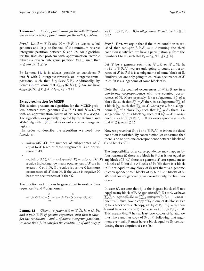
Theorem 6   An ℓ-approximation for the RMCISP prob-lem ensures a 4.5ℓ-approximation for the IRTD problem.

Proof Let G = (S, S) and H = (P, P) be two co-tailed genomes and let p be the size of the minimum reverse intergenic partition between G and H . An algorithm for the RMCISP problem with approximation factor ℓ returns a reverse intergenic partition (S,P) , such that p ≤ cost(S,P) ≤ ℓp.

By Lemma  11, it is always possible to transform G into H with k intergenic reversals or intergenic trans-positions, such that k ≤ 3

2 cost(S,P) . Additionally, by Lemma  6, we know that dIRT (G,H) ≥

p3 . So, we have

dIRT (G,H) ≤ k ≤ 4.5ℓdIRT (G,H) . �

2k‑approximation for MCISPThis section presents an algorithm for the MCISP prob-lem between two genomes G = (S, S) and H = (P, P) with an approximation factor of 2k, where k = occ(S) . The algorithm was partially inspired by the Kolman and Waleń algorithm [20] that does not consider intergenic regions.

In order to describe the algorithm we need two functions:

• subgen(G,X ) : the number of subgenomes of G equal to X (each of these subgenomes is an occur-rence of X).

• weight(G,H,X ) = subgen(G,X )− subgen(H,X ) : a value indicating how many occurrences of X are in excess in G or in H . If the value is positive G has more occurrences of X than H . If the value is negative H has more occurrences of X than G.

The function weight can be generalized to work on two sequences S and P of genomes:

Lemma 12   Given two genomes G = (S, S) , H = (P, P) , and a pair (S,P) of genome sequences, such that it satis-fies the conditions 1 and 2 of direct intergenic partition, we have that (S,P) satisfies the condition 3 if and only if

weight(S,P,X ) =

|S|∑

i=1

subgen(Si ,X )−

|P|∑

i=1

subgen(Pi ,X )

weight(S,P,X ) = 0 for all genomes X contained in G or in H.

Proof First, we argue that if the third condition is sat-isfied then weight(S,P,X ) = 0 . Assuming the third condition is satisfied, we have a permutation φ , from the numbers 1 to |S| , such that Pi = Sφi , ∀ 1 ≤ i ≤ |S|.

Let X be a genome such that X ⊂ G or X ⊂ H . In weight(S,P,X ) , we are only going to count an occur-rence of X in G if it is a subgenome of some block of S . Similarly, we are only going to count an occurrence of X in H if it is a subgenome of some block of P.

Note that, the counted occurrences of X in G are in a one-to-one correspondence with the counted occur-rences of H . More precisely, for a subgenome Si,jk of a block Sk , such that Si,jk = X there is a subgenome Pi,j

φk of

a block Pφk , such that Pi,jφk

= X . Conversely, for a subge-nome Pi,j

φk of a block Pφk , such that Pi,j

φk= X , there is a

subgenome Si,jk of a block Sk , such that Si,jk = X . Conse-quently, weight(S,P,X ) = 0 , for every genome X , such that X ⊂ G or X ⊂ H.

Now we prove that if weight(S,P,X ) = 0 then the third condition is satisfied. By contradiction let us assume that there is no one-to-one correspondence between blocks of S and blocks of P.

The impossibility of a correspondence may happen by four reasons: (i) there is a block in S that is not equal to any block of P ; (ii) there is a genome X correspondent to r blocks of S , but ℓ < r blocks of P ; (iii) there is a block in P not equal to any block of S ; (iv) there is a genome X correspondent to r blocks of P , but ℓ < r blocks of S . Without loss of generality, we consider only the first two cases.

In case (i), assume that Sj is the biggest block of S not equal to any block of P . As weight(S,P, Sj) = 0 , we have ∑|S|

i=1 subgen(Si, Sj) =∑|P|

i=1 subgen(Pi, Sj) . Conse-quently, P must have a copy of Sj in one of its blocks. Let Ps be a block with such copy, i.e., Sj ⊂ Ps . If Ps = Sj , then S must have a copy of Ps , because weight(S,P,Ps) = 0 . This means that S has at least two copies of Sj and we must have another copy of Sj in P . Following that argu-ment eventually P must have a block equal to Sj , contra-dicting the assumption of case (i).

Page 13 of 23Siqueira et al. Algorithms Mol Biol (2021) 16:21

In case (ii) we can establish a correspondence between the ℓ blocks of P and some of the r blocks of S . We have at least one block of S without a correspondent in P . If we ignore the blocks with correspondences when calculating the weights, the same argument of case (i) leads to a con-tradiction. �

Given two genomes G and H , we can easily construct a pair of genomes sequences (S,P) satisfying the first two conditions of direct intergenic partition. We just have to choose which intergenic regions of G and H will be the breakpoints of S and P , respectively. By Lemma  12, to ensure that (S,P) is a direct intergenic partition of G and H , we must choose the breakpoints such that weight(S,P,X ) = 0 for all genomes X of G or H.

Let TG,H be the set of all genomes X , such that X ⊂ G or X ⊂ H , and weight(G,H,X ) = 0 and consider the subset T

minG,H = {X ∈ TG,H|Y �⊂ X , ∀Y ∈ TG,H,Y �= X } .

Note that, to include a breakpoint in some occurrence of a genome Y ∈ TG,H \ Tmin

G,H , it suffices to include a breakpoint in the correspondent occurrence of a genome X ∈ T

minG,H,X ⊂ Y . For that reason, we start by including

breakpoints in elements of TminG,H . In fact, the following

lemma ensures that we must include at least one break-point for each element of Tmin

G,H.

Lemma 13 In order to construct a direct intergenic par-tition (S,P) of two genomes G and H , we must include a breakpoint in at least one copy of every element X ∈ T

minG,H.

Proof For a genome X ∈ TG,H , let k = weight(G,H,X ) . To ensure that weight(S,P,X ) = 0 , if k > 0 then we must include breakpoints in at least k copies of X in G , otherwise, if k < 0 , we must include breakpoints in at least −k copies of X in H . As weight(G,H,X ) = 0 , we must include at least one breakpoint in G or in H , and the lemma follows. �

It may be necessary to include a breakpoint in more than one occurrence of a genome X ∈ T

minG,H . We define

break(X ) as the breakpoint associated with the genome X , and when we include a breakpoint in an occurrence of X we always select a breakpoint equivalent to break(X ).

To include the breakpoints, we not only must know the genomes contained in G or H with initially non-zero weight, but also keep track of genomes that acquire a non-zero weight after the inclusion of a breakpoint. For that, we generalize the sets TG,H and Tmin

G,H to con-sider genome sequences. Given two genome sequences S and P , the set TS,P comprises of genomes X , such

that X ⊂ Si , for 1 ≤ i ≤ |S| , or X ⊂ Pj , for 1 ≤ j ≤ |P| , and weight(S,P,X ) = 0 . Additionally, we have the set Tmin

S,P = {X ∈ TS,P|Y �⊂ X , ∀Y ∈ TS,P,Y �= X }.Let us define break(X ) for a genome X ∈ T

min

S,P . If X ∈ T

minG,H , break(X ) is already defined, otherwise, there

must be at least one breakpoint included in some occur-rence of X in G or H , so break(X ) is equivalent to the first breakpoint included in some occurrence of X .

The algorithm that selects the breakpoints (Algo-rithm  1) works as follows. Initially we consider two sequences S0 = [G] and P0 = [H] , each with a single block. At the i-th step, we produce the sequences Si and Pi including a breakpoint in the sequences Si−1 and Pi−1 based on the following rules:

• The breakpoint is included in an occurrence of a genome X ∈ T

min

Si−1,Pi−1.• If weight(Si−1,Pi−1,X ) > 0 , the selected occur-

rence of X must come from G.• If weight(Si−1,Pi−1,X ) < 0 , the selected occur-

rence of X must come from H.• The selected breakpoint must be equivalent to

break(X ).

The algorithm continues until weight(Si,Pi,X ) = 0 for all genomes X of G or H , i.e., until (Si,Pi) becomes a direct intergenic partition.

Let us briefly discuss the time complexity of Algo-rithm 1. Let n be the size of the input strings. First, we consider the complexity to build Tmin

G,H . Using the suffix tree data structure [29] (constructed in time O(n)), subgen(G,X ) is computed in O(n) time, and, conse-quently, so is weight(G,H,X ) . Similarly, for a genome Y , we can recover the genomes X contained in G or H , such that Y ⊂ X , in O(n) time. Since there are 2n2 subge-nomes of G and H , the set Tmin

G,H can be constructed in O(n3) time. We can also store which subgenomes belong to the set Tmin

Si ,Pi in a suffix tree allowing the update of

Tmin

Si ,Pi in O(n) time. Additionally, we can store the known

breakpoints in a binary search tree so it is possible to recover break(X ) in O(n log n) time. The initialization of Algorithm 1 (lines 1 to 4) takes O(n3) time, the loop from lines 5 to 16 is repeated at most O(n) times, because there are at most 2n breakpoints, and each iteration takes at most O(n log n) time, since searching the breakpoint takes time O(n log n) and updating Tmin

Si ,Pi takes linear

time. Consequently, Algorithm  1 has time complexity O(n3).

Page 14 of 23Siqueira et al. Algorithms Mol Biol (2021) 16:21

Example 3

Execution of Algorithm  1 with genomes G = (S, S) and H = (P, P) . In a genome X , the intergenic region corre-spondent to break(X ) is marked in bold.

S = [I B A B C B C F ] S = [1 3 2 3 1 3 2]

P = [I B C A B B C F ] P = [1 3 0 2 4 3 2]

Tmin

G,H = {([B A], [3]), ([A B C], [2 3]), ([C B], [1]),

(([I B C], [1 3])[C A], [0]), ([B B], [4])}

S0 = [([I B ABC BC F ], [1 3 2 3 1 3 2])]

P0 = [([I B C ABBC F ], [1 3 0 2 4 3 2])]

Tmin

S0 ,P0= T

min

G,H

S1 = [([I B], [1]) ([ABC BC F ], [2 3 1 3 2])]

P1 = P0

Tmin

S1,P1= {([A B C], [2 3]), ([C B], [1]), ([I B C], [1 3]),

([C A], [0]), ([B B], [4])}

S2 = [([I B], [1]) ([A], [ ]) ([BC BC F ], 3 1 3 2)]

P2 = P1

Tmin

S2 ,P2= {([C B], [1]), ([I B C], [1 3]), ([C A], [0]),

([B B], [4]), ([A B], [2])}

S3 = [([I B], [1]) ([A], [ ]) ([BC], [3]),

([BC F ], [3 2])]

P3 = P2

Tmin

S3,P3= {([I B C], [1 3]), ([C A], [0]), ([B B], [4]),

([A B], [2])}

S4 = S3

P4 = [([I], [ ]) ([BC ABBC F ], [3 0 2 4 3 2])]

Tmin

S4 ,P4= {([C A], [0]), ([B B], [4]), ([A B], [2]),

([I B], [1])}

S5 = S4

P5 = [([I], [ ]) ((BC), [3]) ([ABBC F ], [2 4 3 2])]

Tmin

S5,P5= {([B B], [4]), ([A B], [2]), ([I B], [1])}

S6 = S5

P6 = [([I], [ ]) ([BC], [3]), ([AB], [2])

([BC F ], [3 2])]

Tmin

S6,P6= {([A B], [2]), ([I B], [1])}

S7 = S6

P7 = [([I], [ ]) ([BC], [3]) ([A], [ ]) ([B], [ ])

([BC F ], [3 2])]

Tmin

S7,P7= {([I B], [1])}

S8 = [([I], [ ]) ([B], [ ]) ([A], [ ]) ([BC], [3])

([BC F ], [3 2])]

P8 = P7

Tmin

S8,P8= {}

Page 15 of 23Siqueira et al. Algorithms Mol Biol (2021) 16:21

Lemma 14 Algorithm  1 produces a direct intergenic partition of two genomes G = (S, S) and H = (P, P) , including at most 2k|Tmin

G,H| breakpoints, where k = occ(S).

Proof Initially, we show that the algorithm stops pro-ducing a direct intergenic partition, i.e., eventually weight(Si,Pi,X ) = 0 . At every step we reduce the occurrence of at least one genome in Si or in Pi and, while weight(Si,Pi,X ) = 0 , there is an element in Tmin

Si ,Pi

where we can insert a breakpoint. As the number of occurrences of genomes in Si and in Pj is finite, integer, non-negative, and always decreasing, eventually the algo-rithm stops with weight(Si,Pi,X ) = 0.

Now, we show that we include at most 2k|TminG,H| break-

points. Every breakpoint is included in an occurrence of a genome from Tmin

G,H or is equivalent to an already included breakpoint. Consequently, every breakpoint is equivalent to break(X ) for some X ∈ T

minG,H . As there is a maximum

of k copies for each gene in G and a maximum of k cop-ies for each gene in H , every breakpoint is equivalent to a maximum of 2k − 1 other breakpoints, so we include at most 2k|Tmin

G,H| breakpoints. �

Theorem  7   Algorithm  1 has an approximation fac-tor of 2k for the MCISP problem between the genomes G = (S, S) and H = (P, P) , where k = occ(S).

Proof Directly from lemmas 13 and 14. �

Corollary 1 Algorithm  1 has an approximation factor of 2k for the MCSP problem between the string S and P, where k = occ(S).

Proof Using the same reduction presented in Theo-rem  2, but considering the optimization versions of the problems, we can apply Algorithm 1 to the MCSP prob-lem and ensure the approximation factor 2k. �

It is worth noting that we improve the previously known �(k) approximation of MCSP [20] from 4k to 2k.

Corollary 2 Algorithm  1, in combination with the algorithm described in Lemma  9, ensures an asymptotic approximation factor of 6k for the ITD problem between the genomes G = (S, S) and H = (P, P) , where k = occ(S).

Proof Directly from theorems 4 and 7. �

2k‑approximation for RMCISPWe can adapt Algorithm  1 to approximate the RMCISP problem. The main point of the adaptation is to use congru-ence of genomes instead of equality and substitute the rela-tion X ⊂ G with a new relation X ⊏ G , such that X ⊏ G if X ⊂ G or rev(X ) ⊂ G . Using this relation, the functions and sets from the previous section must be adapted:

• subgen(G,X ) is now the number of subgenomes of G congruent to X (i.e., equal to X or to rev(X ) ). Con-sequently, weight considers now this new subgen function.

• TG,H is now the set of all genomes X , such that X ⊏ G or X ⊏ H , and weight(G,H,X ) = 0 . Additionally, TminG,H = {X ∈ TG,H|Y �⊏ X , ∀Y ∈ TG,H,Y �= X }

( Tmin

S,P is adapted in a similar manner).

Some other adaptations must be made on Algorithm 1. Line 5 must check if (S,P) is a reverse intergenic partition instead of a direct intergenic partition. In lines 9 and 13, the block must contain an occurrence of X or rev(X ) , and the break-point in lines 10 and 14 must be congruent to break(X ) instead of equivalent to break(X ) . Next, we show analo-gous results to the ones presented in the previous section.

Lemma 15   Given two genomes G = (S, S) , H = (P, P) , and a pair (S,P) of genome sequences, such that it satis-fies conditions 1 and 2 of reverse intergenic partition, we have that (S,P) satisfies condition 3 if and only if weight(S,P,X ) = 0 for all genomes X , such that X ⊏ G or X ⊏ H.

Proof First, we argue that if the third condition is sat-isfied then weight(S,P,X ) = 0 . Assuming the third condition is satisfied, we have a permutation φ , from the numbers 1 to |S| , such that Pi

∼= Sφi , ∀ 1 ≤ i ≤ |S|.

Let X be a genome such that X ⊏ G or X ⊏ H . In weight(S,P,X ) , we are only going to count an occur-rence of X or rev(X ) in G if it is a subgenome of some block of S . Similarly, we are only going to count an occurrence of X or rev(X ) in H if it is a subgenome of some block of P.

Note that the counted occurrences of X or rev(X ) in G are in a one-to-one correspondence with the counted occurrences in H . More precisely, for a subgenome Si,jk of a block Sk such that Si,jk ∼= X , there is a subgenome Pi,j

φk

of a block Pφk , such that Pi,jφk

∼= X . Conversely, for a sub-genome Pi,j

φk of a block Pφk , such that Pi,j

φk∼= X there is a

Page 16 of 23Siqueira et al. Algorithms Mol Biol (2021) 16:21

subgenome Si,jk of a block Sk , such that Si,jk ∼= X . Conse-quently, weight(S,P,X ) = 0 for every genome X , such that X ⊏ G or X ⊏ H.

Now we prove that if weight(S,P,X ) = 0 then the third condition is satisfied. By contradiction let us assume that there is no one-to-one correspondence between blocks of S and blocks of P.

The impossibility of a correspondence may happen by four reasons: (i) there is a block in S that is not congruent to any block of P ; (ii) there is a genome X congruent to r blocks of S , but it is congruent to ℓ < r blocks of P ; (iii) there is a block in P not congruent to any block of S ; (iv) there is a genome X congruent to r blocks of P , but it is congruent to ℓ < r blocks of S . Without loss of generality, we consider only the first two cases.

In case (i), assume that Sj is the biggest block of S not congruent to any block of P . As weight(S,P, Sj) = 0 , we have

∑|S|i=1 subgen(Si, Sj) =

∑|P|i=1 subgen(Pi, Sj) . Con-

sequently, P must have a copy of Sj or rev(Sj) in one of its blocks. Let Ps be a block with such copy, i.e., Sj ⊏ Ps . If Ps ∼= Sj , then S must have a copy of Ps or rev(Ps ), because weight(S,P,Ps) = 0 . This means that S has at least two copies of Sj or rev(Sj) and we must have another copy of Sj or rev(Sj) in P . Following that argument, eventually P must have a block equal to Sj or rev(Sj) , contradicting the assumption of case (i).

In case (ii) we can establish a correspondence between the ℓ blocks of P and some of the r blocks of S . We have at least one block of S without a correspondent in P . If we ignore the blocks with correspondences when calculating the weights, the same argument of case (i) leads to a con-tradiction. �

Lemma 16 In order to construct a reverse inter-genic partition (S,P) of two genomes G and H , we must include a breakpoint in at least one copy of every element X ∈ T

minG,H.

Proof For a genome X ∈ TG,H , let k = weight(G,H,X ) . To ensure that weight(S,P,X ) = 0 , if k > 0 , then we must include breakpoints in at least k copies of X or rev(X ) in G , other-wise, if k < 0 , we must include breakpoints in at least −k copies of X or rev(X ) in H . As weight(G,H,X ) = 0 , we must include at least one breakpoint in G or in H , and the lemma follows. �

Lemma 17 The adaptation of Algorithm  1 produces a direct intergenic partition of two genomes G = (S, S) and H = (P, P) , including at most 2k|Tmin

G,H| breakpoints, where k = occ(S).

Proof We know the algorithm stops producing a reverse intergenic partition for the same reason stated in Lemma  14. Additionally, every breakpoint is included in an occurrence of a genome from Tmin

G,H or is congruent to an already included breakpoint. Consequently, every breakpoint is congruent to break(X ) for some X ∈ T

minG,H .

As there is a maximum of k copies for each gene in G and a maximum of k copies for each gene in H , every breakpoint is congruent to a maximum of 2k − 1 other breakpoints, so we include at most 2k|Tmin

G,H| breakpoints. �

Theorem  8 The adaptation of Algorithm  1 has an approximation factor of 2k for the RMCISP problem between the genomes G = (S, S) and H = (P, P) , where k = occ(S).

Proof Directly from lemmas 16 and 17. �

Corollary 3 The adaptation of Algorithm  1 has an approximation factor of 2k for the RMCSP problem between the string S and P, where k = occ(S).

Proof Applying a reduction, as in Corollary  1, we can apply the adaptation of Algorithm 1 to the RMCSP prob-lem and ensure the approximation factor 2k. �

It is worth noting that we improve the previously known �(k) approximation of RMCSP [20] from 8k to 2k.

Corollary 4 The adaptation of Algorithm  1 combined with the algorithm described by Brito et  al. [24] for the Sorting Permutations by Intergenic Reversals problem ensures an approximation factor of 8k for the IRD prob-lem between the strings S and P, where k = occ(S).

Proof Directly from theorems 5 and 8. �

Corollary 5 The adaptation of Algorithm  1 com-bined with the algorithm described by Brito et  al. [24] for the Sorting Permutations by Intergenic Reversals and Transpositions problem ensures an approximation fac-tor of 9k for the IRTD problem between the genomes G = (S, S) and H = (P, P) , where k = occ(S).

Proof Directly from theorems 6 and 8. �

Page 17 of 23Siqueira et al. Algorithms Mol Biol (2021) 16:21

Experimental resultsThis section presents the results of our algorithms applied in databases of simulated genomes. Our partition algorithm was implemented in Haskell and the experi-ments were conducted on a PC equipped with a 2.3GHz Intel® Xeon® CPU E5-2470 v2, with 40 cores and 32 GB of RAM, running Ubuntu 18.04.2. We constructed one database for each rearrangement model: TRANS for intergenic transpositions, REV for intergenic reversals, and REVTRANS for intergenic reversals and transpo-sitions. Each database has 40 sets of 100 genome pairs, and each set is defined by the size m of its correspondent alphabet and a number o of applied operations. Each pair of genomes was constructed as follows:

1 For the source genome G = (S, S) , we constructed the string S by selecting 100 characters from a uni-form distribution of m characters (correspondent to an alphabet � , such that �S ⊂ � ), each charac-ter could be selected more than once. Afterwards, we constructed the list S by randomly choosing each intergenic region from integers in the interval [0,  100], each integer had the same probability of being chosen.

2 For the target genome H = (P, P) , we apply o opera-tions in S. The type of operation depends on the database. In the TRANS database, we applied o inter-genic transpositions τ (i,j,k)(x,y,z) , where the values of i, j, k, x, y, and z were randomly chosen. In the REV data-base, we applied o intergenic reversals ρ(i,j)

(x,y) , where the values i, j, x, and y were randomly chosen. In the REVTRANS database we applied

⌊

o2

⌋

intergenic reversals and

⌈

o2

⌉

intergenic transpositions. These operations were aplied in a random order and the parameters of each one were randomly chosen.

3 We performed the extension process by adding two extra characters in the extremities of the source and target genomes to ensure that they are co-tailed. Note that both genomes have a final size of 102.

In these tests, for each pair of genomes from the TRANS database, we computed the direct intergenic partition from our algorithm, and for each pair of genomes from REV and TRANSREV databases, we computed the reverse intergenic partition from our algorithm. After-wards, we produced 100 orthologous assignments capa-ble of inducing each partition. We ensured that each possible assignment had the same probability of being chosen.

For each assignment, we computed the distance between the genomes using the assignment. The dis-tances are computed by a different algorithm for each

database: for the TRANS database, we used the algorithm described in Lemma  9 (implemented in C++); for the REV and REVTRANS databases, we used the algorithms for reversals and reversals and transpositions from Brito et al. [24] (implemented in Python), respectively.

To compare with the distances that do not consider the partitions, we also produced, for each genome pair, 100 assignments that do not take into account the partitions. We computed the distances for each of these assignments as well.

Tables 2, 3, and 4 show the distances for the TRANS, REV, and REVTRANS databases, respectively. Each line corresponds to a set of 100 genome pairs; the first two columns indicate, respectively, the number of operations and the size of the alphabet used to generated the set. The following seven columns present the results consid-ering the partitions. For each genome pair, we consider the minimum and average distance from all 100 assign-ments. For each set, we report the minimum (Min.), aver-age (Avg.), and maximum (Max.) for those two values. We also report the average time, in seconds, necessary to produce the partition and compute the 100 distances. The last seven columns present the same values for the distances that do not consider the partitions. In that case, the time reported refers only to calculating the distances.

Figures  8,  9, and  10 show box plots with the average distances for the TRANS, REV, and REVTRANS data-bases, respectively.

From Table  2 and Fig.  8, we see that in the TRANS database the distances considering the partitions are lower than the distances that do not take the partitions into account. For sets generated with 25 transpositions, the minimum distances without partition are, on average, at least 39% higher than the minimum distances with par-tition. For the average distance, the difference is at least 60% on average. The difference between the distances decreases as the number of operations or the size of the alphabet increases. For sets generated with 100 transpo-sitions and alphabet of size 10, the minimum and aver-age distances without partition are on average 8% higher than the minimum or average distances with partition. For sets generated with 100 transpositions and alphabet of size 100, the minimum distances without partition are on average 3% higher than the minimum distances with partition. For the average distance, the difference is 5% on average. It is worth mentioning that with 100 operations we have an extreme case, where each origin genome is considerably shuffled to produce the corre-sponding target genome of the pair. It is also interesting that with smaller alphabets, when the number of repli-cas increases, the advantage of using the partitions also increases. Looking at the running times, we see that, for

Page 18 of 23Siqueira et al. Algorithms Mol Biol (2021) 16:21

the transposition model, we must pay a small cost to pro-duce better distances using the partitions.

From Table 3 and Fig. 9, we see that in the REV data-base the distances considering the partitions are still lower than the distances that do not take the partitions

into account, and the differences between distances are higher for this database. For sets generated with 25 rever-sals, the minimum distances without partition are, on average, at least 149% higher than the minimum distances with partition. For the average distance, the difference is

Table 2 Distances for the ITD problem with and without the use of our partition algorithm

OP |�| With partition Without partition

Minimum distance Average distance Time Minimum distance Average distance Time

Min. Avg. Max. Min. Avg. Max. Min. Avg. Max. Min. Avg. Max.

25 10 42 47.83 57 43.64 49.45 58.80 0.22 94 96.91 98 99.93 100.19 100.52 0.02

25 20 38 48.07 61 39.85 49.61 61.79 0.22 88 93.42 96 97.99 98.63 99.41 0.01

25 30 39 47.85 55 40.71 49.27 56.62 0.22 84 88.89 92 94.72 96.27 97.49 0.02

25 40 39 48.53 57 40.85 49.91 58.67 0.22 77 84.97 88 89.56 93.60 95.62 0.01

25 50 41 48.38 55 42.54 49.59 56.87 0.22 69 81.20 87 86.35 90.66 93.87 0.01

25 60 40 48.56 57 40.68 49.69 58.79 0.23 70 77.84 84 81.71 88.00 93.21 0.01

25 70 40 47.94 54 40.42 48.85 55.96 0.22 68 74.88 84 80.36 85.60 91.40 0.01

25 80 40 48.29 56 40.00 49.20 57.03 0.23 62 71.84 78 77.62 83.26 88.35 0.01

25 90 39 48.53 55 39.57 49.36 56.89 0.22 61 70.86 81 74.31 81.82 88.77 0.01

25 100 41 48.85 56 41.25 49.61 56.80 0.23 58 68.29 77 71.95 79.51 86.20 0.01

50 10 64 71.52 80 65.79 73.08 80.86 0.33 96 98.03 99 100.20 100.46 100.80 0.01

50 20 63 72.17 80 65.62 73.68 81.79 0.33 92 95.51 98 98.71 99.57 100.30 0.02

50 30 66 72.38 82 67.76 73.86 83.79 0.32 90 93.19 96 96.83 98.40 99.75 0.01

50 40 62 71.98 82 63.84 73.55 82.87 0.33 85 91.14 95 93.56 96.89 99.07 0.02

50 50 62 72.25 80 63.70 73.74 80.97 0.33 84 89.44 94 92.76 95.60 98.03 0.01

50 60 60 71.51 81 61.97 73.01 82.74 0.33 82 87.18 92 89.80 94.03 97.91 0.01

50 70 64 71.96 80 65.64 73.56 81.80 0.33 79 85.89 90 87.46 92.80 95.79 0.01

50 80 65 72.04 83 65.81 73.66 84.78 0.33 78 84.64 91 87.05 91.79 96.90 0.01

50 90 62 71.64 80 62.70 73.14 80.91 0.33 76 83.25 90 84.45 90.39 95.29 0.01

50 100 65 72.04 82 65.90 73.52 83.85 0.34 75 82.74 89 83.25 89.98 94.72 0.01

75 10 76 84.41 92 77.53 86.00 93.90 0.38 96 98.26 100 100.23 100.58 100.82 0.02

75 20 76 84.71 91 77.65 86.28 91.91 0.38 94 96.95 99 99.50 100.15 100.54 0.01

75 30 76 84.36 92 76.83 85.91 92.88 0.38 92 95.52 98 97.47 99.39 100.43 0.01

75 40 79 84.87 92 80.75 86.43 93.70 0.39 91 94.51 97 97.46 98.76 100.09 0.02

75 50 77 85.04 95 78.83 86.67 95.83 0.38 90 93.66 98 94.47 98.02 100.16 0.02

75 60 76 84.01 91 77.66 85.55 92.80 0.38 89 92.21 96 94.24 97.07 99.44 0.01

75 70 79 84.99 92 80.71 86.48 93.80 0.38 86 92.01 95 90.84 96.64 98.65 0.01

75 80 77 85.06 93 78.92 86.63 94.82 0.39 86 91.26 96 92.84 95.90 98.98 0.01

75 90 74 85.41 93 76.85 86.93 94.78 0.40 85 90.93 97 90.58 95.78 99.25 0.01

75 100 74 84.52 94 74.70 86.12 94.78 0.39 81 90.00 96 89.03 95.05 98.69 0.01

100 10 82 90.80 96 83.72 92.40 96.86 0.41 97 98.68 100 100.43 100.67 100.94 0.02

100 20 83 91.23 97 84.71 92.87 98.91 0.41 95 97.87 99 99.57 100.41 100.83 0.02

100 30 86 91.55 97 87.74 93.15 98.84 0.41 95 97.33 99 98.93 100.10 100.72 0.02

100 40 86 91.72 98 87.81 93.25 98.80 0.42 94 96.58 99 98.53 99.72 100.60 0.02

100 50 84 91.17 98 85.83 92.71 99.77 0.42 91 95.73 99 96.15 99.13 100.72 0.02

100 60 85 91.49 98 86.77 92.96 99.72 0.42 90 95.18 99 95.77 98.74 100.24 0.02

100 70 83 91.54 98 84.67 93.07 99.76 0.42 86 95.05 99 91.77 98.41 100.60 0.01

100 80 84 91.20 99 85.67 92.81 99.77 0.42 90 94.40 99 95.22 98.01 100.50 0.01

100 90 87 91.49 96 87.56 93.10 97.81 0.43 91 94.35 98 95.19 97.87 100.10 0.01

100 100 86 91.71 98 87.85 93.21 98.85 0.43 91 94.16 98 94.98 97.65 100.33 0.01

Page 19 of 23Siqueira et al. Algorithms Mol Biol (2021) 16:21

at least 173% on average. Again, the difference between the distances decreases as the number of operations or the size of the alphabet increases, however, even in sets generated with 100 reversals and alphabet of size 100, the minimum distances with partition are on average

14% higher than the minimum distances with partition. For the average distance, the difference is 16% on aver-age. In the REV database, we see that the running time considering the partition was lower than the running time without the partition. This happened because the

Table 3 Distances for the IRD problem with and without the use of our partition algorithm

OP |�| With partition Without Partition

Minimum Distance Average Distance Time Minimum Distance Average Distance Time

Min. Avg. Max. Min. Avg. Max. Min. Avg. Max. Min. Avg. Max.

25 10 27 33.38 41 30.65 37.20 47.07 5.35 98 100.44 102 105.15 105.84 106.82 14.43

25 20 27 32.64 38 29.44 35.36 41.36 5.11 93 98.04 101 102.56 104.56 105.80 14.21

25 30 28 32.55 38 29.25 34.90 40.69 4.99 88 95.02 99 99.35 102.59 104.50 13.83

25 40 28 32.91 39 28.00 34.65 40.48 4.98 84 92.17 98 95.01 100.47 104.07 13.71

25 50 28 32.62 38 28.00 34.13 39.42 4.96 80 89.46 96 92.96 98.65 102.58 13.26

25 60 27 32.61 39 27.00 33.85 40.81 4.94 78 87.57 98 91.02 97.03 104.22 12.99

25 70 28 32.35 39 28.00 33.64 40.90 4.93 73 85.74 94 87.39 95.04 101.30 12.71

25 80 27 32.69 38 28.04 33.58 39.50 4.97 72 83.86 95 84.09 93.49 101.54 12.40

25 90 27 32.79 38 27.00 33.55 40.39 4.94 72 82.31 92 82.03 91.70 99.34 12.03

25 100 28 32.78 38 28.00 33.48 39.24 4.92 66 81.82 95 80.16 91.52 101.39 12.04

50 10 54 60.94 68 56.67 64.24 71.66 9.38 98 100.83 103 105.48 106.04 106.86 14.48

50 20 52 59.96 68 55.80 63.24 72.77 9.29 97 99.30 101 103.80 105.11 106.16 14.37

50 30 51 59.91 70 53.45 63.03 73.07 9.22 92 97.56 100 101.59 104.05 106.35 14.19

50 40 51 59.86 68 53.22 62.93 71.84 9.28 90 95.72 100 99.79 102.76 104.98 13.93

50 50 50 59.70 67 51.83 62.82 71.34 9.08 89 94.04 100 97.50 101.47 104.42 13.73

50 60 54 59.69 67 55.81 62.55 69.59 9.13 84 92.74 99 93.63 100.16 105.08 13.44

50 70 52 59.48 65 54.02 62.42 69.31 9.02 84 91.46 98 92.73 99.12 103.50 13.34

50 80 51 59.30 68 53.04 62.05 71.22 8.91 83 90.18 97 91.74 97.89 103.89 13.12

50 90 53 59.65 66 55.03 62.23 68.75 9.01 79 89.12 95 89.68 96.90 102.52 12.99

50 100 51 58.68 65 53.30 61.24 68.84 8.96 77 88.71 98 86.47 96.52 102.28 13.00

75 10 67 75.02 81 69.82 78.41 83.89 11.51 99 101.33 103 105.40 106.17 106.67 14.52

75 20 67 75.19 83 70.95 78.60 86.92 11.43 97 99.94 102 104.55 105.55 106.39 14.35

75 30 67 74.70 83 70.08 78.23 86.72 11.56 94 98.79 102 103.79 104.89 106.20 14.33

75 40 68 75.63 82 70.68 79.10 85.96 11.53 93 98.20 101 101.55 104.17 105.73 14.23

75 50 68 74.52 82 70.73 77.93 84.80 11.37 89 96.76 100 99.61 103.13 105.25 14.08

75 60 67 75.07 84 71.77 78.33 88.08 11.44 90 95.81 100 98.14 102.43 105.60 13.87

75 70 63 75.03 85 65.25 78.32 88.19 11.44 86 95.35 100 97.33 101.91 105.08 14.00

75 80 67 74.70 81 69.33 77.70 84.76 11.31 86 94.74 99 95.42 101.16 105.35 13.65

75 90 68 74.97 82 70.67 77.94 85.61 11.50 87 94.00 99 96.41 100.67 106.91 13.73

75 100 65 74.49 82 69.30 77.59 85.82 11.18 84 93.34 100 92.97 99.93 103.94 13.48

100 10 77 83.54 91 80.65 87.27 95.42 13.12 98 101.23 103 105.77 106.25 106.79 14.56

100 20 77 83.34 90 80.43 87.14 93.44 12.89 97 100.65 103 104.04 105.80 106.69 14.45

100 30 75 83.73 91 78.56 87.41 94.77 13.17 97 99.67 102 102.77 105.30 106.59 14.39

100 40 77 83.78 92 79.85 87.43 96.10 12.89 94 98.77 101 100.29 104.46 106.72 14.20

100 50 76 83.76 91 80.52 87.36 95.46 13.02 94 98.42 102 100.86 104.17 106.55 14.25

100 60 77 84.05 91 79.73 87.58 95.06 13.12 93 97.50 101 99.96 103.51 105.93 14.05

100 70 77 84.40 92 79.93 87.91 95.21 12.97 93 97.38 101 99.26 103.16 106.34 14.03

100 80 76 83.95 92 79.82 87.46 95.58 12.95 91 96.94 101 97.99 102.77 105.72 13.91

100 90 77 84.10 93 80.15 87.50 97.68 12.84 93 96.56 101 99.07 102.37 106.41 13.80

100 100 74 84.09 90 76.45 87.45 93.49 13.02 89 96.41 101 96.20 102.10 105.84 13.87

Page 20 of 23Siqueira et al. Algorithms Mol Biol (2021) 16:21

100 runs of the distance algorithm were slower than the partition algorithm, and using assignments that consider the partition tends to reduce the running time of the dis-tance algorithm as the number of breakpoints tends to

be smaller than the number of breakpoints considering a random assignment.

From Table  4 and Fig.  10, we see that in the REVTRANS database the distances considering the

Table 4 Distances for the IRTD problem with and without the use of our partition algorithm

OP |�| With partition Without partition

Minimum distance Average distance Time Minimum distance Average distance Time

Min. Avg. Max. Min. Avg. Max. Min. Avg. Max. Min. Avg. Max.

25 10 34 42.01 52 35.07 43.70 52.51 6.86 95 97.08 98 99.61 100.12 100.50 12.59

25 20 32 41.89 50 32.53 43.38 51.06 6.74 91 94.79 98 97.78 99.10 99.84 12.53

25 30 34 41.79 48 34.74 43.18 49.83 6.76 85 92.07 96 95.73 97.69 99.68 12.39

25 40 34 41.39 47 35.55 42.60 48.38 6.78 81 89.38 94 91.59 95.91 98.63 12.31

25 50 35 41.97 48 35.00 43.03 50.70 6.68 79 87.64 94 89.88 94.51 98.58 12.28

25 60 37 41.65 48 37.00 42.60 48.27 6.64 77 85.67 93 87.68 93.16 97.16 12.07

25 70 34 41.73 49 34.98 42.68 49.44 6.73 73 82.57 92 85.13 90.79 97.24 11.84

25 80 37 42.26 49 37.54 43.05 50.05 6.83 69 81.44 89 79.81 89.54 95.94 11.73

25 90 35 41.57 48 35.76 42.34 48.57 6.62 71 79.51 89 79.79 87.65 95.32 11.54

25 100 35 41.84 48 36.00 42.57 49.22 6.71 66 79.31 89 77.86 87.45 94.45 11.43

50 10 59 66.72 75 60.61 67.91 76.42 10.13 95 97.64 99 99.91 100.26 100.50 12.59

50 20 57 66.93 74 58.60 68.14 74.67 10.03 94 96.08 98 98.93 99.63 100.39 12.50

50 30 60 67.11 76 61.56 68.25 77.61 10.10 90 94.31 97 97.01 98.73 99.85 12.45

50 40 56 66.21 73 56.47 67.35 74.62 9.97 86 92.72 96 95.12 97.72 99.91 12.36

50 50 59 66.79 74 60.41 67.96 75.60 10.04 87 91.76 96 94.44 96.98 99.49 12.29

50 60 57 66.32 75 57.74 67.39 76.48 10.12 81 89.80 94 92.17 95.72 98.76 12.33

50 70 53 66.66 75 53.77 67.86 76.61 9.88 83 89.43 95 88.72 94.97 98.51 12.16

50 80 59 66.69 72 59.68 67.74 73.50 9.84 77 88.68 95 89.37 94.34 98.27 12.25

50 90 53 66.24 75 54.56 67.30 76.58 10.09 80 87.89 94 87.04 93.64 97.91 12.16

50 100 59 66.36 76 59.44 67.33 76.59 9.85 80 87.03 94 87.12 92.81 96.63 12.06

75 10 71 79.44 86 72.64 80.61 86.68 11.86 96 97.82 99 100.07 100.35 100.61 12.62

75 20 74 79.92 88 74.53 81.05 88.75 11.84 95 96.88 99 98.85 99.94 100.45 12.55

75 30 71 79.72 87 72.55 80.99 88.57 11.94 92 95.69 98 97.62 99.37 100.19 12.50

75 40 69 79.47 88 70.51 80.64 89.64 11.84 90 94.72 97 96.37 98.67 99.91 12.43

75 50 70 80.38 88 70.72 81.49 89.60 12.00 86 93.89 97 95.04 98.09 100.15 12.44

75 60 72 80.04 89 72.59 81.13 89.67 11.88 88 93.55 97 94.59 97.71 99.60 12.43

75 70 72 80.72 89 72.52 81.78 89.68 12.00 88 92.89 97 93.54 97.06 99.82 12.29

75 80 71 79.91 89 72.68 81.05 89.76 11.86 87 91.95 97 93.33 96.27 99.12 12.44

75 90 73 79.81 88 73.65 80.84 88.63 11.98 88 91.74 96 92.58 96.00 99.04 12.37

75 100 73 80.26 89 73.63 81.32 90.53 11.84 85 91.36 96 90.71 95.55 99.20 12.18

100 10 80 86.23 95 80.56 87.44 96.71 13.20 97 98.18 99 100.13 100.42 100.72 12.62

100 20 81 86.61 94 81.70 87.78 94.59 13.26 95 97.20 99 99.28 100.09 100.56 12.54

100 30 79 87.14 93 80.63 88.39 93.81 13.29 94 96.59 98 98.59 99.73 100.30 12.59

100 40 80 87.15 92 81.57 88.31 93.67 13.19 93 95.84 98 97.28 99.29 100.17 12.50

100 50 79 86.92 93 80.53 88.02 94.68 13.18 91 95.26 97 96.09 98.81 100.18 12.47

100 60 79 87.14 93 80.47 88.27 94.56 13.15 90 94.89 98 96.08 98.52 100.15 12.42

100 70 81 87.61 92 82.67 88.71 93.64 13.21 90 94.70 98 94.98 98.21 100.08 12.37

100 80 78 87.98 96 79.69 89.09 96.57 13.47 91 94.55 97 95.46 98.01 99.97 12.50

100 90 79 87.04 93 80.66 88.22 93.65 13.16 89 94.14 97 93.84 97.64 99.72 12.32

100 100 78 87.46 93 80.53 88.50 94.68 13.13 88 93.65 98 92.55 97.19 100.04 12.24

Page 21 of 23Siqueira et al. Algorithms Mol Biol (2021) 16:21

partitions are still lower than the distances that do not take the partitions into account. The differences were higher than those from the TRANS database, but smaller than those from the REV database. For sets generated with 25 operations, the minimum distances without par-tition are, on average, at least 90% higher than the mini-mum distances with partition. For the average distance, the difference is at least 105% on average. Again, the dif-ference between the distances decreases as the number of operations or the size of the alphabet increases. In sets

generated with 100 operations and alphabet of size 100, the minimum distances with partition are on average 7% higher than the minimum distances with partition. For the average distance, the difference is 10% on average. For the set generated with at most 75 operations, the running time considering the partition was lower than the run-ning time without the partition.

Considering all results, we see that the partitions improve the distances and the improvement is higher for

With Partition Without Partition

25 50 75 100 25 50 75 1000

25

50

75

100

Applied Operations (OP)

Aver

age

Dis

tanc

e

Fig. 8 Average distances for the ITD problem with and without the use of our partition algorithm

With Partition Without Partition

25 50 75 100 25 50 75 1000

30

60

90

Applied Operations (OP)

Aver

age

Dis

tanc

e

Fig. 9 Average distances for the IRD problem with and without the use of our partition algorithm

Page 22 of 23Siqueira et al. Algorithms Mol Biol (2021) 16:21

smaller alphabets or closer genomes (genomes that can be turned into one another with fewer operations). We can also see that with partitions, we have either a small cost in the running time, when the distance algorithm takes less time than the partition algorithm, or a large gain in running time, when the distance algorithm takes more time than the partition algorithm.

ConclusionWe defined the intergenic transposition distance (ITD), the intergenic reversal distance (IRD), the intergenic reversal and transposition distance (IRTD), the minimum common intergenic string partition (MCISP), and the reverse minimum com-mon intergenic string partition (RMCISP) prob-lems. Next, we described a relation between the partition and distance problems and a �(k)-approximation for the MCISP and RMCISP problems ensuring a �(k)-approxi-mation for the ITD, IRD, and IRTD problems. Our algo-rithm for the MCISP and RMCISP problems may also be applied to the MCSP and RMCSP problems, which do not consider intergenic regions, improving a previously known approximation. We also performed practical tests on simulated genomes, showing that the distances calcu-lated considering the partitions were lower than the dis-tances calculated without taking partitions into account.

As future works, one can extend our approach by con-sidering the orientation of the genes. Additionally, one possible approach to overcome the balanced genome restriction is to consider non-conservative events, such as insertion and deletion, similarly to the work of

Alexandrino et al. [30] with the Intergenic Reversal Dis-tance without gene repetition.

AcknowledgementsThis work was supported by the National Council of Technological and Scientific Development, CNPq (Grant 425340/2016-3), the Coordenação de Aperfeiãoamento de Pessoal de Nível Superior - Brasil (CAPES) - Finance Code 001, and the São Paulo Research Foundation, FAPESP (Grants 2013/08293-7, 2015/11937-9, 2017/12646-3, and 2019/27331-3).

Authors contributionsFirst draft: GS. Proofs: GS, AOA, and ARO. Final manuscript: GS, AOA, ARO, and ZD. All authors read and approved the final manuscript.

Availability of data and materialsThe algorithms and datasets generated during the current study are available in the following public repository: https:// github. com/ compb iogro up/ Appro ximat ion- Algor ithm- for- Rearr angem ent- Dista nces- Consi dering- Repea ted- Genes- and- Inter genic- Region.

Declarations

Competing interestsThe authors declare that they have no competing interests.

Received: 26 June 2021 Accepted: 31 August 2021

References 1. Willing E, Stoye J, Braga MD. Computing the Inversion-Indel Distance.

IEEE/ACM transactions on computational biology and bioinformatics. 2020.

2. Kahn C, Raphael B. Analysis of segmental duplications via duplication distance. Bioinformatics. 2008;24(16):i133–8.

3. Abdullah T, Faiza M, Pant P, Rayyan Akhtar M, Pant P. An analysis of single nucleotide substitution in genetic codons–probabilities and outcomes. Bioinformation. 2016;12(3):98–104.

With Partition Without Partition

25 50 75 100 25 50 75 1000

25

50

75

100

Applied Operations (OP)

Aver

age

Dis

tanc

e

Fig. 10 Average distances for the IRTD problem with and without the use of our partition algorithm

Page 23 of 23Siqueira et al. Algorithms Mol Biol (2021) 16:21

• fast, convenient online submission

•

thorough peer review by experienced researchers in your field

• rapid publication on acceptance

• support for research data, including large and complex data types

•

gold Open Access which fosters wider collaboration and increased citations

maximum visibility for your research: over 100M website views per year •

At BMC, research is always in progress.

Learn more biomedcentral.com/submissions

Ready to submit your researchReady to submit your research ? Choose BMC and benefit from: ? Choose BMC and benefit from:

4. Fertin G, Labarre A, Rusu I, Tannier É, Vialette S. Combinatorics of genome rearrangements. Computational molecular biology. London: The MIT Press; 2009.

5. Bergeron A, Mixtacki J, Stoye J. A Unifying View of Genome Rearrange-ments. In: International Workshop on Algorithms in Bioinformatics. Springer; 2006. p. 163–73.

6. Sankoff D. Genome rearrangement with gene families. Bioinformatics. 1999;15(11):909–17.

7. Chen X, Zheng J, Fu Z, Nan P, Zhong Y, Lonardi S, et al. Assignment of orthologous genes via genome rearrangement. IEEE/ACM Trans Comput Biol Bioinform. 2005;2(4):302–15.

8. Siqueira G, Brito KL, Dias U, Dias Z. Heuristics for Genome Rearrangement Distance with Replicated Genes. IEEE/ACM Transactions on Computa-tional Biology and Bioinformatics. 2021; p. 1.

9. Biller P, Guéguen L, Knibbe C, Tannier E. Breaking good: accounting for fragility of genomic regions in rearrangement distance estimation. Genome Biol Evol. 2016;8(5):1427–39.

10. Biller P, Knibbe C, Beslon G, Tannier E. Comparative Genomics on Artificial Life. In: Pursuit of the Universal. Springer International Publishing; 2016. p. 35–44.

11. Bulteau L, Fertin G, Rusu I. Sorting by transpositions is difficult. SIAM J Discrete Math. 2012;26(3):1148–80.

12. Elias I, Hartman TA. 1.375-approximation algorithm for sorting by transpo-sitions. IEEE/ACM Trans Comput Biol Bioinfor. 2006;3(4):369–79.

13. Caprara A. Sorting permutations by reversals and eulerian cycle decom-positions. SIAM J Discrete Math. 1999;12(1):91–110.

14. Berman P, Hannenhalli S, Karpinski M. 1.375-Approximation Algorithm for Sorting by Reversals. In: Proceedings of the 10th Annual European Symposium on Algorithms (ESA’2002). vol. 2461 of Lecture Notes in Computer Science. Springer-Verlag Berlin Heidelberg New York; 2002. p. 200–210.

15. Hannenhalli S, Pevzner PA. Transforming cabbage into turnip: polyno-mial algorithm for sorting signed permutations by reversals. J ACM. 1999;46(1):1–27.

16. Oliveira AR, Brito KL, Dias U, Dias Z. On the complexity of sorting by reversals and tanspositions problems. J Comput Biol. 2019;26:1223–9.

17. Rahman A, Shatabda S, Hasan M. An approximation algorithm for sorting by reversals and transpositions. J Discrete Algorithms. 2008;6(3):449–57.

18. Chen X. On sorting unsigned permutations by double-cut-and-joins. J Combinatorial Optim. 2013;25(3):339–51.

19. Walter MEMT, Dias Z, Meidanis J. Reversal and Transposition Distance of Linear Chromosomes. In: Proceedings of the 5th International Sympo-sium on String Processing and Information Retrieval (SPIRE’1998). Los Alamitos, CA, USA: IEEE Computer Society; 1998. p. 96–102.

20. Kolman P, Waleń T. Reversal Distance for Strings with Duplicates: Linear Time Approximation Using Hitting Set. In: Proceedings of the 4th Interna-tional Workshop on Approximation and Online Algorithms (WAOA’2006). Springer Berlin Heidelberg; 2007. p. 279–289.

21. Shapira D, Storer JA. Edit distance with move operations. Journal of Discrete Algorithms. 2007;5(2):380–92.

22. Radcliffe AJ, Scott AD, Wilmer EL. Reversals and transpositions over finite alphabets. SIAM J Discrete Math. 2005;19(1):224–44.

23. Oliveira AR, Jean G, Fertin G, Brito KL, Dias U, Dias Z. A 3.5-Approximation Algorithm for Sorting by Intergenic Transpositions. In: Algorithms for Computational Biology. Springer International Publishing; 2020. p. 16–28.

24. Brito KL, Jean G, Fertin G, Oliveira AR, Dias U, Dias Z. Sorting by genome rearrangements on both gene order and intergenic sizes. J Comput Biol. 2020;27(2):156–74.

25. Oliveira AR, Jean G, Fertin G, Brito KL, Dias U, Dias Z. Sorting Permutations by Intergenic Operations. IEEE/ACM Transactions on Computational Biol-ogy and Bioinformatics. 2021; p. 1.

26. Kolman P, Waleń T. Approximating reversal distance for strings with bounded number of duplicates. Discrete Appl Math. 2007;155(3):327–36.

27. Cormode G, Muthukrishnan S. The string edit distance matching problem with moves. ACM Trans Algorithms. 2007;3(1):1–19.

28. Goldstein A, Kolman P, Zheng J. Minimum Common String Partition Problem: Hardness and Approximations. In: Proceedings of the 15th International Symposium on Algorithms and Computation (ISAAC’2004). Springer Berlin Heidelberg; 2005. p. 484–495.

29. Crochemore M, Lecroq T. Suffix Tree. In: Encyclopedia of Database Sys-tems. US: Springer; 2009. p. 2876–80.

30. Alexandrino AO, Brito KL, Oliveira AR, Dias U, Dias Z. Reversal Distance on Genomes with Different Gene Content and Intergenic Regions Informa-tion. In: Algorithms for Computational Biology. vol. 12715. Springer International Publishing; 2021. p. 121–133.

Publisher’s NoteSpringer Nature remains neutral with regard to jurisdictional claims in pub-lished maps and institutional affiliations.