APPROXIMATE UNIVERSAL ARTIFICIAL Doctor of Philosophy

A P P R O X I M AT E U N I V E R S A L A RT I F I C I A LI N T E L L I G E N C E A N D S E L F - P L AY L E A R N I N G

F O R G A M E S

Doctor of Philosophy Dissertation

School of Computer Science and Engineering

joel veness

supervisors

Kee Siong NgMarcus Hutter

Alan BlairWilliam Uther

John Lloyd

January 2011

Joel Veness: Approximate Universal Artificial Intelligence andSelf-play Learning for Games, Doctor of Philosophy Disserta-tion, © January 2011

When we write programs that learn, it turns out that we do and they don’t.

— Alan Perlis

A B S T R A C T

This thesis is split into two independent parts.

The first is an investigation of some practical aspects of Marcus Hutter’s Uni-

versal Artificial Intelligence theory [29]. The main contributions are to show how

a very general agent can be built and analysed using the mathematical tools of

this theory. Before the work presented in this thesis, it was an open question as to

whether this theory was of any relevance to reinforcement learning practitioners.

This work suggests that it is indeed relevant and worthy of future investigation.

The second part of this thesis looks at self-play learning in two player, determin-

istic, adversarial turn-based games. The main contribution is the introduction of

a new technique for training the weights of a heuristic evaluation function from

data collected by classical game tree search algorithms. This method is shown

to outperform previous self-play training routines based on Temporal Difference

learning when applied to the game of Chess. In particular, the main highlight was

using this technique to construct a Chess program that learnt to play master level

Chess by tuning a set of initially random weights from self play games.

iii

P U B L I C AT I O N S

A significant portion of the technical content of this thesis has been previously

published at leading international Artificial Intelligence conferences and peer-

reviewed journals.

The relevant material for Part I includes:

• Reinforcement Learning via AIXI Approximation, [82]

Joel Veness, Kee Siong Ng, Marcus Hutter, David Silver

Association for the Advancement of Artificial Intelligence (AAAI), 2010.

• A Monte-Carlo AIXI Approximation, [83]

Joel Veness, Kee Siong Ng, Marcus Hutter, William Uther, David Silver

Journal of Artificial Intelligence Research (JAIR), 2010.

The relevant material for Part II includes:

• Bootstrapping from Game Tree Search [81]

Joel Veness, David Silver, Will Uther, Alan Blair

Neural Information Processing Systems (NIPS), 2009.

v

We should not only use the brains we have, but all that we can borrow.

— Woodrow Wilson

A C K N O W L E D G M E N T S

Special thanks to Kee Siong for all his time, dedication and encouragement. This

work would not have been possible without him. Thanks to Marcus for having the

courage to both write his revolutionary book and take me on late as a PhD student.

Thanks to Alan, John and Will for many helpful discussions and suggestions.

Finally, a collective thanks to all of my supervisors for letting me pursue my own

interests.

Thankyou to UNSW and NICTA for the financial support that allowed me to

write this thesis and attend a number of overseas conferences. Thankyou to Peter

Cheeseman for giving me my first artificial intelligence job. Thanks to my external

collaborators, in particular David Silver and Shane Legg. Thankyou to Michael

Bowling and the University of Alberta for letting me finish my thesis on campus.

Thankyou to the external examiners for their constructive feedback.

Thankyou to the international cricket community for years of entertainment.

Thankyou to the few primary, secondary and university teachers who kept me

interested. Thankyou to the science fiction community for being a significant

source of inspiration, in particular Philip K. Dick, Ursula Le Guin, Frederik Pohl,

Robert Heinlein and Vernor Vinge.

Thankyou to my family, and in particular my mother, who in spite of significant

setbacks managed to ultimately do a good job. Thankyou to my friends for all

the good times. Thankyou to my fiancée Felicity for her love and support. Finally,

thanks to everyone who gave a word or two of encouragement along the way.

vii

D E C L A R AT I O N

I hereby declare that this submission is my own work and to the best of my knowl-

edge it contains no materials previously published or written by another person,

or substantial proportions of material which have been accepted for the award

of any other degree or diploma at UNSW or any other educational institution,

except where due acknowledgment is made in the thesis. Any contribution made

to the research by others, with whom I have worked at UNSW or elsewhere, is

explicitly acknowledged in the thesis. I also declare that the intellectual content

of this thesis is the product of my own work, except to the extent that assistance

from others in the project’s design and conception or in style, presentation and

linguistic expression is acknowledged.

Joel Veness

C O N T E N T S

i approximate universal artificial intelligence 1

1 reinforcement learning via aixi approximation 3

1.1 Overview 3

1.2 Introduction 4

1.2.1 The General Reinforcement Learning Problem 4

1.2.2 The AIXI Agent 5

1.2.3 AIXI as a Principle 6

1.2.4 Approximating AIXI 6

1.3 The Agent Setting 7

1.3.1 Agent Setting 7

1.3.2 Reward, Policy and Value Functions 8

1.4 Bayesian Agents 10

1.4.1 Prediction with a Mixture Environment Model 11

1.4.2 Theoretical Properties 12

1.4.3 AIXI: The Universal Bayesian Agent 14

1.4.4 Direct AIXI Approximation 14

2 expectimax approximation 16

2.1 Background 16

2.2 Overview 17

2.3 Action Selection at Decision Nodes 19

2.4 Chance Nodes 20

2.5 Estimating Future Reward at Leaf Nodes 21

2.6 Reward Backup 21

2.7 Pseudocode 22

xi

xii contents

2.8 Consistency of ρUCT 25

2.9 Parallel Implementation of ρUCT 25

3 model class approximation 26

3.1 Context Tree Weighting 26

3.1.1 Krichevsky-Trofimov Estimator 27

3.1.2 Prediction Suffix Trees 28

3.1.3 Action-conditional PST 30

3.1.4 A Prior on Models of PSTs 31

3.1.5 Context Trees 32

3.1.6 Weighted Probabilities 34

3.1.7 Action Conditional CTW as a Mixture Environment

Model 35

3.2 Incorporating Type Information 36

3.3 Convergence to the True Environment 38

3.4 Summary 41

3.5 Relationship to AIXI 42

4 putting it all together 43

4.1 Convergence of Value 43

4.2 Convergence to Optimal Policy 45

4.3 Computational Properties 48

4.4 Efficient Combination of FAC-CTW with ρUCT 48

4.5 Exploration/Exploitation in Practice 49

4.6 Top-level Algorithm 50

5 results 51

5.1 Empirical Results 51

5.1.1 Domains 51

5.1.2 Experimental Setup 57

5.1.3 Results 61

contents xiii

5.1.4 Discussion 64

5.1.5 Comparison to 1-ply Rollout Planning 65

5.1.6 Performance on a Challenging Domain 67

5.2 Discussion 69

5.2.1 Related Work 69

5.2.2 Limitations 71

6 future work 73

6.1 Future Scalability 73

6.1.1 Online Learning of Rollout Policies for ρUCT 73

6.1.2 Combining Mixture Environment Models 75

6.1.3 Richer Notions of Context for FAC-CTW 75

6.1.4 Incorporating CTW Extensions 76

6.1.5 Parallelization of ρUCT 77

6.1.6 Predicting at Multiple Levels of Abstraction 77

6.2 Conclusion 77

6.3 Closing Remarks 78

ii learning from self-play using game tree search 79

7 bootstrapping from game tree search 81

7.1 Overview 81

7.2 Introduction 82

7.3 Background 83

7.4 Minimax Search Bootstrapping 86

7.5 Alpha-Beta Search Bootstrapping 88

7.5.1 Updating Parameters in TreeStrap(αβ) 90

7.5.2 The TreeStrap(αβ) algorithm 90

7.6 Learning Chess Program 91

7.7 Experimental Results 92

7.7.1 Relative Performance Evaluation 93

xiv contents

7.7.2 Evaluation by Internet Play 95

7.8 Conclusion 97

bibliography 99

L I S T O F F I G U R E S

Figure 1 A ρUCT search tree 19

Figure 2 An example prediction suffix tree 29

Figure 3 A depth-2 context tree (left). Resultant trees after processing

one (middle) and two (right) bits respectively. 33

Figure 4 The MC-AIXI agent loop 50

Figure 5 The cheese maze 53

Figure 6 A screenshot (converted to black and white) of the PacMan

domain 56

Figure 7 Average Reward per Cycle vs Experience 63

Figure 8 Performance versus ρUCT search effort 64

Figure 9 Online performance on a challenging domain 67

Figure 10 Scaling properties on a challenging domain 68

Figure 11 Online performance when using a learnt rollout policy on

the Cheese Maze 74

Figure 12 Left: TD, TD-Root and TD-Leaf backups. Right: Root-

Strap(minimax) and TreeStrap(minimax). 84

Figure 13 Performance when trained via self-play starting from ran-

dom initial weights. 95% confidence intervals are marked at

each data point. The x-axis uses a logarithmic scale. 94

xv

L I S T O F TA B L E S

Table 1 Domain characteristics 52

Table 2 Binary encoding of the domains 58

Table 3 MC-AIXI(fac-ctw) model learning configuration 59

Table 4 U-Tree model learning configuration 61

Table 5 Resources required for (near) optimal performance by MC-

AIXI(fac-ctw) 62

Table 6 Average reward per cycle: ρUCT versus 1-ply rollout plan-

ning 66

Table 7 Backups for various learning algorithms. 87

Table 8 Best performance when trained by self play. 95% confidence

intervals given. 95

Table 9 Blitz performance at the Internet Chess Club 96

xvi

Part I

A P P R O X I M AT E U N I V E R S A L A RT I F I C I A L

I N T E L L I G E N C E

Beware the Turing tar-pit, where everything is possible but nothing of interest is easy.

— Alan Perlis

1R E I N F O R C E M E N T L E A R N I N G V I A A I X I A P P R O X I M AT I O N

1.1 overview

This part of the thesis introduces a principled approach for the design of a

scalable general reinforcement learning agent. The approach is based on a direct

approximation of AIXI, a Bayesian optimality notion for general reinforcement

learning agents. Previously, it has been unclear whether the theory of AIXI could

motivate the design of practical algorithms. We answer this hitherto open question

in the affirmative, by providing the first computationally feasible approximation to

the AIXI agent. To develop our approximation, we introduce a new Monte-Carlo

Tree Search algorithm along with an agent-specific extension to the Context Tree

Weighting algorithm. Empirically, we present a set of encouraging results on a

variety of stochastic and partially observable domains, including a comparison

to two existing general agent algorithms, U-Tree [44] and Active-LZ [17]. We

conclude by proposing a number of directions for future research.

3

4 reinforcement learning via aixi approximation

1.2 introduction

Reinforcement Learning is a popular and influential paradigm for agents that

learn from experience. Whilst there are many different ways this paradigm can

be formalised, all approaches seem to involve accepting the so-called reward

hypothesis, namely: “that all of what we mean by goals and purposes can be well

thought of as maximization of the expected value of the cumulative sum of a received

scalar reward signal."1 From an agent design perspective, this hypothesis suggests a

normative model for agent behaviour. Popular reinforcement learning formalisms

that capture this notion include Markov Decision Processes (MDPs) [51] and

Partially Observable Markov Decision Processes (POMDPs) [31].

This chapter explores the practical ramifications of a different Reinforcement

Learning formalism. The setup in question was introduced by Marcus Hutter,

in his Universal Artificial Intelligence work [29]. Like previous approaches, this

theory also captures the reward hypothesis. What distinguishes the formalism

however is that it is explicitly designed for agents that learn history based, proba-

bilistic models of the environment.

The main highlight of this part of the thesis will be the construction of a real-

world agent built from and analysed using the AIXI theory. Although the material

presented in this part is self contained, some prior exposure to Reinforcement

Learning or Bayesian statistics would be helpful.

1.2.1 The General Reinforcement Learning Problem

Consider an agent that exists within some unknown environment. The agent

interacts with the environment in cycles. In each cycle, the agent executes an action

and in turn receives an observation and a reward. The only information available

1 http://rlai.cs.ualberta.ca/RLAI/rewardhypothesis.html

http://rlai.cs.ualberta.ca/RLAI/rewardhypothesis.html

1.2 introduction 5

to the agent is its history of previous interactions. The general reinforcement learning

problem is to construct an agent that, over time, collects as much reward as possible

from the (unknown) environment.

1.2.2 The AIXI Agent

The AIXI agent is a mathematical solution to the general reinforcement learning

problem. To achieve generality, the environment is assumed to be an unknown

but computable function; i.e. the observations and rewards received by the agent,

given its past actions, can be computed by some program running on a Turing

machine. The AIXI agent results from a synthesis of two ideas:

1. the use of a finite-horizon expectimax operation from sequential decision

theory for action selection; and

2. an extension of Solomonoff’s universal induction scheme [69] for future

prediction in the agent context.

More formally, let U(q,a1a2 . . . an) denote the output of a universal Turing ma-

chine U supplied with program q and input a1a2 . . . an, m ∈N a finite lookahead

horizon, and `(q) the length in bits of program q. The action picked by AIXI at

time t, having executed actions a1a2 . . . at−1 and having received the sequence of

observation-reward pairs o1r1o2r2 . . . ot−1rt−1 from the environment, is given by:

a∗t = arg maxat

∑otrt

. . .maxat+m

∑ot+mrt+m

[rt + · · ·+ rt+m]∑

q:U(q,a1...at+m)=o1r1...ot+mrt+m

2−`(q). (1.1)

Intuitively, the agent considers the sum of the total reward over all possible

futures up to m steps ahead, weights each of them by the complexity of programs

consistent with the agent’s past that can generate that future, and then picks the

action that maximises expected future rewards. Equation (1.1) embodies in one

line the major ideas of Bayes, Ockham, Epicurus, Turing, von Neumann, Bellman,


Kolmogorov, and Solomonoff. The AIXI agent is rigorously shown by [29] to be

optimal in many different senses of the word. In particular, the AIXI agent will

rapidly learn an accurate model of the environment and proceed to act optimally

to achieve its goal.

Accessible overviews of the AIXI agent have been given by both Legg [37] and

Hutter [30]. A complete description of the agent can be found in [29].

1.2.3 AIXI as a Principle

As the AIXI agent is only asymptotically computable, it is by no means an

algorithmic solution to the general reinforcement learning problem. Rather it is

best understood as a Bayesian optimality notion for decision making in general

unknown environments. As such, its role in general AI research should be viewed

in, for example, the same way the minimax and empirical risk minimisation

principles are viewed in decision theory and statistical machine learning research.

These principles define what is optimal behaviour if computational complexity

is not an issue, and can provide important theoretical guidance in the design of

practical algorithms. This thesis demonstrates, for the first time, how a practical

agent can be built from the AIXI theory.

1.2.4 Approximating AIXI

As can be seen in Equation (1.1), there are two parts to AIXI. The first is the

expectimax search into the future which we will call planning. The second is the

use of a Bayesian mixture over Turing machines to predict future observations

and rewards based on past experience; we will call that learning. Both parts

need to be approximated for computational tractability. There are many different

approaches one can try. In this attempt, we opted to use a generalised version

1.3 the agent setting 7

of the UCT algorithm [32] for planning and a generalised version of the Context

Tree Weighting algorithm [89] for learning.

1.3 the agent setting

This section introduces the notation and terminology we will use to describe

strings of agent experience, the true underlying environment and the agent’s

model of the true environment.

notation. A string x1x2 . . . xn of length n is denoted by x1:n. The prefix x1:j of

x1:n, j 6 n, is denoted by x6j or x<j+1. The notation generalises for blocks of sym-

bols: e.g. ax1:n denotes a1x1a2x2 . . . anxn and ax<j denotes a1x1a2x2 . . . aj−1xj−1.

The empty string is denoted by ε. The concatenation of two strings s and r is

denoted by sr.

1.3.1 Agent Setting

The (finite) action, observation, and reward spaces are denoted by A,O, and R

respectively. Also, X denotes the joint perception space O×R.

Definition 1. A history h is an element of (A×X)∗ ∪ (A×X)∗ ×A.

The following definition states that the environment takes the form of a prob-

ability distribution over possible observation-reward sequences conditioned on

actions taken by the agent.

Definition 2. An environment ρ is a sequence of conditional probability functions

{ρ0, ρ1, ρ2, . . . }, where ρn : An → Density (Xn), that satisfies

∀a1:n∀x<n : ρn−1(x<n |a<n) =∑xn∈X

ρn(x1:n |a1:n). (1.2)


In the base case, we have ρ0(ε | ε) = 1.

Equation (1.2), called the chronological condition in [29], captures the natural

constraint that action an has no effect on earlier perceptions x<n. For convenience,

we drop the index n in ρn from here onwards.

Given an environment ρ, we define the predictive probability

ρ(xn |ax<nan) :=ρ(x1:n |a1:n)

ρ(x<n |a<n)(1.3)

∀a1:n∀x1:n such that ρ(x<n |a<n) > 0. It now follows that

ρ(x1:n |a1:n) = ρ(x1 |a1)ρ(x2 |ax1a2) · · · ρ(xn |ax<nan). (1.4)

Definition 2 is used in two distinct ways. The first is a means of describing the

true underlying environment. This may be unknown to the agent. Alternatively,

we can use Definition 2 to describe an agent’s subjective model of the environment.

This model is typically learnt, and will often only be an approximation to the true

environment. To make the distinction clear, we will refer to an agent’s environment

model when talking about the agent’s model of the environment.

Notice that ρ(· |h) can be an arbitrary function of the agent’s previous history h.

Our definition of environment is sufficiently general to encapsulate a wide variety

of environments, including standard reinforcement learning setups such as MDPs

or POMDPs.

1.3.2 Reward, Policy and Value Functions

We now cast the familiar notions of reward, policy and value [76] into our setup.

The agent’s goal is to accumulate as much reward as it can during its lifetime.

More precisely, the agent seeks a policy that will allow it to maximise its expected

future reward up to a fixed, finite, but arbitrarily large horizon m ∈ N. The

1.3 the agent setting 9

instantaneous reward values are assumed to be bounded. Formally, a policy is

a function that maps a history to an action. If we define Rk(aor6t) := rk for

1 6 k 6 t, then we have the following definition for the expected future value of

an agent acting under a particular policy:

Definition 3. Given history ax1:t, the m-horizon expected future reward of an agent

acting under policy π : (A×X)∗ → A with respect to an environment ρ is:

vmρ (π,ax1:t) := Eρ

[t+m∑i=t+1

Ri(ax6t+m)

∣∣∣∣ x1:t]

, (1.5)

where for t < k 6 t +m, ak := π(ax<k). The quantity vmρ (π,ax1:tat+1) is defined

similarly, except that at+1 is now no longer defined by π.

The optimal policy π∗ is the policy that maximises the expected future reward.

The maximal achievable expected future reward of an agent with history h in

environment ρ looking m steps ahead is Vmρ (h) := vmρ (π∗,h). It is easy to see that

if h ∈ (A×X)t, then

Vmρ (h) = maxat+1

∑xt+1

ρ(xt+1 |hat+1)maxat+2

∑xt+2

ρ(xt+2 |hat+1xt+1at+2) · · ·

maxat+m

∑xt+m

ρ(xt+m |haxt+1:t+m−1at+m)

[t+m∑i=t+1

ri

]. (1.6)

For convenience, we will often refer to Equation (1.6) as the expectimax operation.

Furthermore, the m-horizon optimal action a∗t+1 at time t+ 1 is related to the

expectimax operation by

a∗t+1 = arg maxat+1

Vmρ (ax1:tat+1). (1.7)

Equations (1.5) and (1.6) can be modified to handle discounted reward, however

we focus on the finite-horizon case since it both aligns with AIXI and allows for a

simplified presentation.


1.4 bayesian agents

As mentioned earlier, Definition 2 can be used to describe the agent’s subjective

model of the true environment. Since we are assuming that the agent does not

initially know the true environment, we desire subjective models whose predictive

performance improves as the agent gains experience. One way to provide such a

model is to take a Bayesian perspective. Instead of committing to any single fixed

environment model, the agent uses a mixture of environment models. This requires

committing to a class of possible environments (the model class), assigning an

initial weight to each possible environment (the prior), and subsequently updating

the weight for each model using Bayes rule (computing the posterior) whenever

more experience is obtained. The process of learning is thus implicit within a

Bayesian setup.

The mechanics of this procedure are reminiscent of Bayesian methods to predict

sequences of (single typed) observations. The key difference in the agent setup

is that each prediction may now also depend on previous agent actions. We

incorporate this by using the action conditional definitions and identities of Section

1.3.

Definition 4. Given a countable model class M := {ρ1, ρ2, . . . } and a prior weight

wρ0 > 0 for each ρ ∈ M such that

∑ρ∈Mw

ρ0 = 1, the mixture environment model is

ξ(x1:n |a1:n) :=∑ρ∈M

wρ0ρ(x1:n |a1:n).

The next proposition allows us to use a mixture environment model whenever

we can use an environment model.

Proposition 1. A mixture environment model is an environment model.

Proof. ∀a1:n ∈ An and ∀x<n ∈ Xn−1 we have that

∑xn∈X

ξ(x1:n |a1:n) =∑xn∈X

∑ρ∈M

wρ0ρ(x1:n |a1:n) =

∑ρ∈M

wρ0

∑xn∈X

ρ(x1:n |a1:n) = ξ(x<n |a<n)

1.4 bayesian agents 11

where the final step follows from application of Equation (1.2) and Definition

4. �

The importance of Proposition 1 will become clear in the context of planning

with environment models, described in Chapter 2.

1.4.1 Prediction with a Mixture Environment Model

As a mixture environment model is an environment model, we can simply use:

ξ(xn |ax<nan) =ξ(x1:n |a1:n)

ξ(x<n |a<n)(1.8)

to predict the next observation reward pair. Equation (1.8) can also be expressed

in terms of a convex combination of model predictions, with each model weighted

by its posterior, from

ξ(xn |ax<nan) =

∑ρ∈M

wρ0ρ(x1:n |a1:n)∑

ρ∈Mwρ0ρ(x<n |a<n)

=∑ρ∈M

wρn−1ρ(xn |ax<nan),

where the posterior weight wρn−1 for environment model ρ is given by

wρn−1 :=

wρ0ρ(x<n |a<n)∑

ν∈Mwν0ν(x<n |a<n)

= Pr(ρ |ax<n) (1.9)

If |M| is finite, Equations (1.8) and (1.4.1) can be maintained online in O(|M|)

time by using the fact that

ρ(x1:n |a1:n) = ρ(x<n |a<n)ρ(xn |ax<na),

which follows from Equation (1.4), to incrementally maintain the likelihood term

for each model.


1.4.2 Theoretical Properties

We now show that if there is a good model of the (unknown) environment in M,

an agent using the mixture environment model

ξ(x1:n |a1:n) :=∑ρ∈M

wρ0ρ(x1:n |a1:n) (1.10)

will predict well. Our proof is an adaptation from Hutter [29]. We present the full

proof here as it is both instructive and directly relevant to many different kinds of

practical Bayesian agents.

First we state a useful entropy inequality.

Lemma 1 (Hutter [29]). Let {yi} and {zi} be two probability distributions, i.e. yi >

0, zi > 0, and∑i yi =

∑i zi = 1. Then we have

∑i

(yi − zi)2 6∑i

yi lnyizi

.

Theorem 1. Let µ be the true environment. The µ-expected squared difference of µ and

ξ is bounded as follows. For all n ∈N, for all a1:n,

n∑k=1

∑x1:k

µ(x<k |a<k)

(µ(xk |ax<kak) − ξ(xk |ax<kak)

)26 minρ∈M

{− lnwρ0 +D1:n(µ ‖ ρ)

},

whereD1:n(µ ‖ ρ) :=∑x1:n

µ(x1:n |a1:n) ln µ(x1:n |a1:n)ρ(x1:n |a1:n)

is the KL divergence of µ(· |a1:n)

and ρ(· |a1:n).

Proof. Combining [29, Thm. 3.2.8 and Thm. 5.1.3] we get

n∑k=1

∑x1:k

µ(x<k |a<k)


)2=

n∑k=1

∑x<k

µ(x<k |a<k)∑xk


)2


6n∑k=1

∑x<k

µ(x<k |a<k)∑xk

µ(xk |ax<kak) lnµ(xk |ax<kak)

ξ(xk |ax<kak)[Lemma 1]

=

n∑k=1

∑x1:k

µ(x1:k |a1:k) lnµ(xk |ax<kak)

ξ(xk |ax<kak)[Equation (1.3)]

=

n∑k=1

∑x1:k

( ∑xk+1:n

µ(x1:n |a1:n)

)lnµ(xk |ax<kak)

ξ(xk |ax<kak)[Equation (1.2)]

=

n∑k=1

∑x1:n

µ(x1:n |a1:n) lnµ(xk |ax<kak)

ξ(xk |ax<kak)

=∑x1:n

µ(x1:n |a1:n)

n∑k=1

lnµ(xk |ax<kak)

ξ(xk |ax<kak)

=∑x1:n

µ(x1:n |a1:n) lnµ(x1:n |a1:n)

ξ(x1:n |a1:n)[Equation (1.4)]

=∑x1:n

µ(x1:n |a1:n) ln[µ(x1:n |a1:n)

ρ(x1:n |a1:n)

ρ(x1:n |a1:n)

ξ(x1:n |a1:n)

][arbitrary ρ ∈M]

=∑x1:n


ρ(x1:n |a1:n)+∑x1:n

µ(x1:n |a1:n) lnρ(x1:n |a1:n)

ξ(x1:n |a1:n)

6 D1:n(µ ‖ ρ) +∑x1:n

µ(x1:n |a1:n) lnρ(x1:n |a1:n)

wρ0ρ(x1:n |a1:n)

[Definition 4]

= D1:n(µ ‖ ρ) − lnwρ0 .

Since the inequality holds for arbitrary ρ ∈M, it holds for the minimising ρ. �

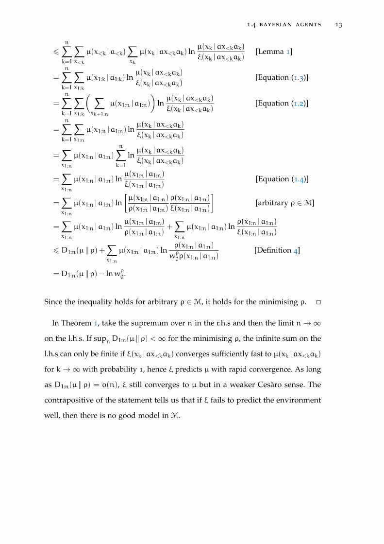
In Theorem 1, take the supremum over n in the r.h.s and then the limit n→∞on the l.h.s. If supnD1:n(µ ‖ ρ) <∞ for the minimising ρ, the infinite sum on the

l.h.s can only be finite if ξ(xk |ax<kak) converges sufficiently fast to µ(xk |ax<kak)

for k→∞ with probability 1, hence ξ predicts µ with rapid convergence. As long

as D1:n(µ ‖ ρ) = o(n), ξ still converges to µ but in a weaker Cesàro sense. The

contrapositive of the statement tells us that if ξ fails to predict the environment

well, then there is no good model in M.


1.4.3 AIXI: The Universal Bayesian Agent

Theorem 1 motivates the construction of Bayesian agents that use rich model

classes. The AIXI agent can be seen as the limiting case of this viewpoint, by using

the largest model class expressible on a Turing machine.

Note that AIXI can handle stochastic environments since Equation (1.1) can be

shown to be formally equivalent to

a∗t = arg maxat

∑otrt

. . .maxat+m

∑ot+mrt+m

[rt + · · ·+ rt+m]∑ρ∈MU

2−K(ρ)ρ(x1:t+m |a1:t+m),

(1.11)

where ρ(x1:t+m |a1 . . . at+m) is the probability of observing x1x2 . . . xt+m given

actions a1a2 . . . at+m, class MU consists of all enumerable chronological semimea-

sures [29], which includes all computable ρ, and K(ρ) denotes the Kolmogorov

complexity [39] of ρ with respect to U. In the case where the environment is a

computable function and

ξU(x1:t |a1:t) :=∑ρ∈MU

2−K(ρ)ρ(x1:t |a1:t), (1.12)

Theorem 1 shows for all n ∈N and for all a1:n,

n∑k=1

∑x1:k

µ(x<k |a<k)

(µ(xk |ax<kak) − ξU(xk |ax<kak)

)26 K(µ) ln 2. (1.13)

1.4.4 Direct AIXI Approximation

We are now in a position to describe our approach to AIXI approximation. For

prediction, we seek a computationally efficient mixture environment model ξ as a

replacement for ξU. Ideally, ξ will retain ξU’s bias towards simplicity and some of


its generality. This will be achieved by placing a suitable Ockham prior over a set

of candidate environment models.

For planning, we seek a scalable algorithm that can, given a limited set of

resources, compute an approximation to the expectimax action given by

a∗t+1 = arg maxat+1

VmξU(ax1:tat+1).

The main difficulties are of course computational. The next two sections in-

troduce two algorithms that can be used to (partially) fulfill these criteria. Their

subsequent combination will constitute our AIXI approximation.

AI is an engineering discipline built on an unfinished science.

– Matt Ginsberg

2E X P E C T I M A X A P P R O X I M AT I O N

Naïve computation of the expectimax operation (Equation 1.6) takesO(|A×X|m)

time, which is unacceptable for all but tiny values of m. This section introduces

ρUCT, a generalisation of the popular Monte-Carlo Tree Search algorithm UCT

[32], that can be used to approximate a finite horizon expectimax operation given

an environment model ρ. As an environment model subsumes both MDPs and

POMDPs, ρUCT effectively extends the UCT algorithm to a wider class of problem

domains.

2.1 background

UCT has proven particularly effective in dealing with difficult problems containing

large state spaces. It requires a generative model that when given a state-action

pair (s,a) produces a subsequent state-reward pair (s ′, r) distributed according

to Pr(s ′, r | s,a). By successively sampling trajectories through the state space, the

UCT algorithm incrementally constructs a search tree, with each node containing

an estimate of the value of each state. Given enough time, these estimates converge

to their true values.

16

2.2 overview 17

The ρUCT algorithm can be realised by replacing the notion of state in UCT by

an agent history h (which is always a sufficient statistic) and using an environment

model ρ to predict the next percept. The main subtlety with this extension is that

now the history condition of the percept probability ρ(or |h) needs to be updated

during the search. This is to reflect the extra information an agent will have at a

hypothetical future point in time. Furthermore, Proposition 1 allows ρUCT to be

instantiated with a mixture environment model, which directly incorporates the

model uncertainty of the agent into the planning process. This gives (in princi-

ple, provided that the model class contains the true environment and ignoring

issues of limited computation) the well known Bayesian solution to the explo-

ration/exploitation dilemma; namely, if a reduction in model uncertainty would

lead to higher expected future reward, ρUCT would recommend an information

gathering action.

2.2 overview

ρUCT is a best-first Monte-Carlo Tree Search technique that iteratively constructs

a search tree in memory. The tree is composed of two interleaved types of nodes:

decision nodes and chance nodes. These correspond to the alternating max and

sum operations in the expectimax operation. Each node in the tree corresponds

to a history h. If h ends with an action, it is a chance node; if h ends with an

observation-reward pair, it is a decision node. Each node contains a statistical

estimate of the future reward.

Initially, the tree starts with a single decision node containing |A| children.

Much like existing MCTS methods [13], there are four conceptual phases to a

single iteration of ρUCT. The first is the selection phase, where the search tree is

traversed from the root node to an existing leaf chance node n. The second is the

expansion phase, where a new decision node is added as a child to n. The third is

18 expectimax approximation

the simulation phase, where a rollout policy in conjunction with the environment

model ρ is used to sample a possible future path from n until a fixed distance

from the root is reached. Finally, the backpropagation phase updates the value

estimates for each node on the reverse trajectory leading back to the root. Whilst

time remains, these four conceptual operations are repeated. Once the time limit

is reached, an approximate best action can be selected by looking at the value

estimates of the children of the root node.

During the selection phase, action selection at decision nodes is done using a

policy that balances exploration and exploitation. This policy has two main effects:

• to gradually move the estimates of the future reward towards the maximum

attainable future reward if the agent acted optimally.

• to cause asymmetric growth of the search tree towards areas that have high

predicted reward, implicitly pruning large parts of the search space.

The future reward at leaf nodes is estimated by choosing actions according to a

heuristic policy until a total of m actions have been made by the agent, where m is

the search horizon. This heuristic estimate helps the agent to focus its exploration

on useful parts of the search tree, and in practice allows for a much larger horizon

than a brute-force expectimax search.

ρUCT builds a sparse search tree in the sense that observations are only added to

chance nodes once they have been generated along some sample path. A full-width

expectimax search tree would not be sparse; each possible stochastic outcome

would be represented by a distinct node in the search tree. For expectimax, the

branching factor at chance nodes is thus |O|, which means that searching to even

moderate sized m is intractable.

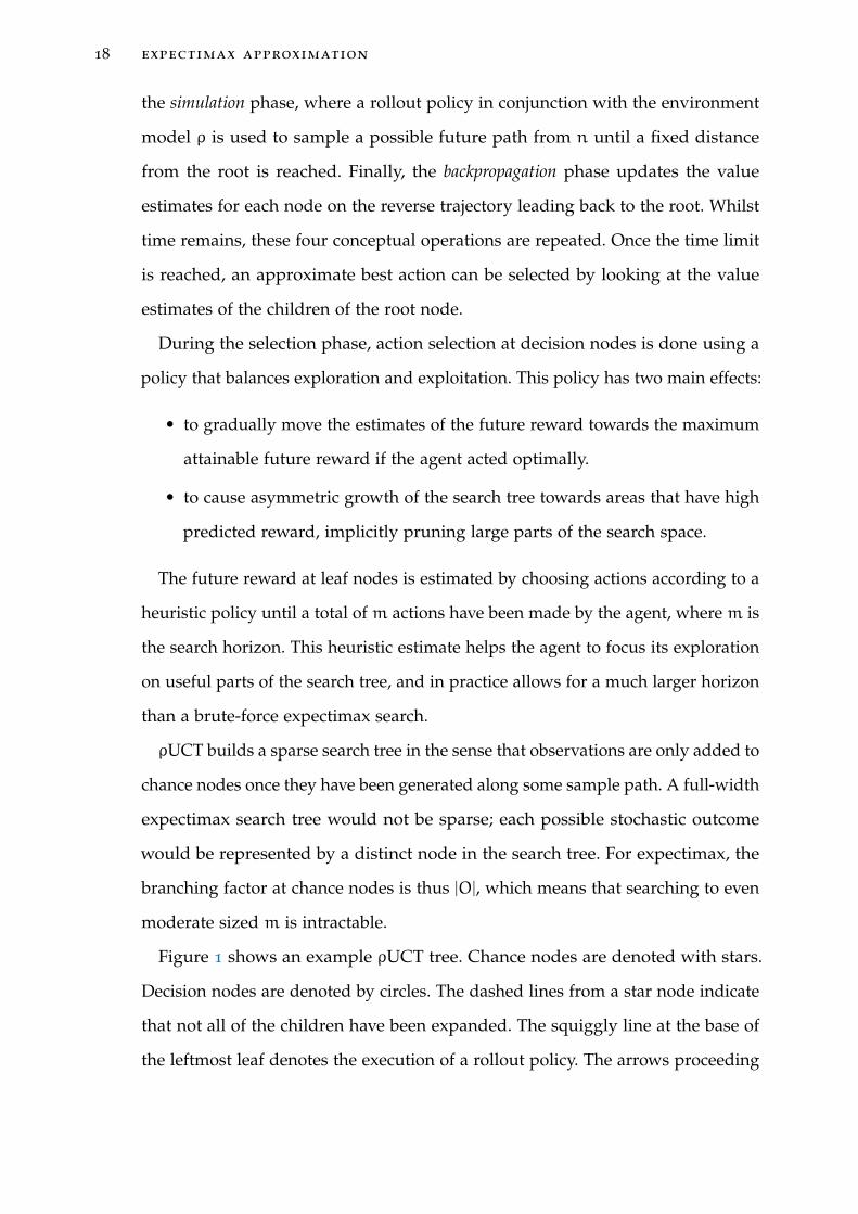
Figure 1 shows an example ρUCT tree. Chance nodes are denoted with stars.

Decision nodes are denoted by circles. The dashed lines from a star node indicate

that not all of the children have been expanded. The squiggly line at the base of

the leftmost leaf denotes the execution of a rollout policy. The arrows proceeding

2.3 action selection at decision nodes 19

a1 a2a3

o1 o2 o3 o4

future reward estimate

Figure 1: A ρUCT search tree

up from this node indicate the flow of information back up the tree; this is defined

in more detail below.

2.3 action selection at decision nodes

A decision node will always contain |A| distinct children, all of whom are chance

nodes. Associated with each decision node representing a particular history h

will be a value function estimate, V(h). During the selection phase, a child will

need to be picked for further exploration. Action selection in MCTS poses a classic

exploration/exploitation dilemma. On one hand we need to allocate enough visits

to all children to ensure that we have accurate estimates for them, but on the

other hand we need to allocate enough visits to the maximal action to ensure

convergence of the node to the value of the maximal child node.

Like UCT, ρUCT recursively uses the UCB policy [1] from the n-armed bandit

setting at each decision node to determine which action needs further exploration.

Although the uniform logarithmic regret bound no longer carries across from the

bandit setting, the UCB policy has been shown to work well in practice in complex

domains such as computer Go [21] and General Game Playing [18]. This policy


has the advantage of ensuring that at each decision node, every action eventually

gets explored an infinite number of times, with the best action being selected

exponentially more often than actions of lesser utility.

Definition 5. The visit count T(h) of a decision node h is the number of times h has

been sampled by the ρUCT algorithm. The visit count of the chance node found by taking

action a at h is defined similarly, and is denoted by T(ha).

Definition 6. Supposem is the remaining search horizon and each instantaneous reward

is bounded in the interval [α,β]. Given a node representing a history h in the search tree,

the action picked by the UCB action selection policy is:

aUCB(h) := arg maxa∈A

1

m(β−α) V(ha) +C√

log(T(h))T(ha) if T(ha) > 0;

∞ otherwise,

(2.1)

where C ∈ R is a positive parameter that controls the ratio of exploration to exploitation.

If there are multiple maximal actions, one is chosen uniformly at random.

Note that we need a linear scaling of V(ha) in Definition 6 because the UCB

policy is only applicable for rewards confined to the [0, 1] interval.

2.4 chance nodes

Chance nodes follow immediately after an action is selected from a decision node.

Each chance node ha following a decision node h contains an estimate of the

future utility denoted by V(ha). Also associated with the chance node ha is a

density ρ(· |ha) over observation-reward pairs.

After an action a is performed at node h, ρ(· |ha) is sampled once to generate

the next observation-reward pair or. If or has not been seen before, the node haor

is added as a child of ha.

2.5 estimating future reward at leaf nodes 21

2.5 estimating future reward at leaf nodes

If a leaf decision node is encountered at depth k < m in the tree, a means of

estimating the future reward for the remainingm−k time steps is required. MCTS

methods use a heuristic rollout policy Π to estimate the sum of future rewards∑mi=k ri. This involves sampling an action a from Π(h), sampling a percept or

from ρ(· |ha), appending aor to the current history h and then repeating this

process until the horizon is reached. This procedure is described in Algorithm 4. A

natural baseline policy is Πrandom, which chooses an action uniformly at random

at each time step.

As the number of simulations tends to infinity, the structure of the ρUCT search

tree converges to the full depth m expectimax tree. Once this occurs, the rollout

policy is no longer used by ρUCT. This implies that the asymptotic value function

estimates of ρUCT are invariant to the choice of Π. In practice, when time is

limited, not enough simulations will be performed to grow the full expectimax

tree. Therefore, the choice of rollout policy plays an important role in determining

the overall performance of ρUCT. Methods for learning Π online are discussed as

future work in Section 6.1. Unless otherwise stated, all of our subsequent results

will use Πrandom.

2.6 reward backup

After the selection phase is completed, a path of nodes n1n2 . . . nk, k 6 m, will

have been traversed from the root of the search tree n1 to some leaf nk. For each

1 6 j 6 k, the statistics maintained for history hnj associated with node nj will be

updated as follows:


V(hnj)←T(hnj)

T(hnj) + 1V(hnj) +

1

T(hnj) + 1

m∑i=j

ri (2.2)

T(hnj)← T(hnj) + 1 (2.3)

Equation (2.2) computes the mean return. Equation (2.3) increments the visit

counter. Note that the same backup operation is applied to both decision and

chance nodes.

2.7 pseudocode

The pseudocode of the ρUCT algorithm is now given.

After a percept has been received, Algorithm 1 is invoked to determine an

approximate best action. A simulation corresponds to a single call to Sample from

Algorithm 1. By performing a number of simulations, a search tree Ψ whose

root corresponds to the current history h is constructed. This tree will contain

estimates Vmρ (ha) for each a ∈ A. Once the available thinking time is exceeded, a

maximising action a∗h := arg maxa∈A Vmρ (ha) is retrieved by BestAction. Impor-

tantly, Algorithm 1 is anytime, meaning that an approximate best action is always

available. This allows the agent to effectively utilise all available computational

resources for each decision.

Algorithm 1 ρUCT(h,m)

Require: A history hRequire: A search horizon m ∈N

1: Initialise(Ψ)2: repeat3: Sample(Ψ,h,m)4: until out of time5: return BestAction(Ψ,h)

For simplicity of exposition, Initialise can be understood to simply clear the

entire search tree Ψ. In practice, it is possible to carry across information from one

2.7 pseudocode 23

time step to another. If Ψt is the search tree obtained at the end of time t, and aor

is the agent’s actual action and experience at time t, then we can keep the subtree

rooted at node Ψt(hao) in Ψt and make that the search tree Ψt+1 for use at the

beginning of the next time step. The remainder of the nodes in Ψt can then be

deleted.

Algorithm 2 describes the recursive routine used to sample a single future

trajectory. It uses the SelectAction routine to choose moves at decision nodes,

and invokes the Rollout routine at unexplored leaf nodes. The Rollout routine

picks actions according to the rollout policy Π until the (remaining) horizon is

reached, returning the accumulated reward. Its pseudocode is given in Algorithm

4. After a complete trajectory of length m is simulated, the value estimates are

updated for each node traversed as per Section 2.6. Notice that the recursive calls

on Lines 6 and 11 of Algorithm 2 append the most recent percept or action to the

history argument.

Algorithm 2 Sample(Ψ,h,m)

Require: A search tree ΨRequire: A history hRequire: A remaining search horizon m ∈N

1: if m = 0 then2: return 0

3: else if Ψ(h) is a chance node then4: Generate (o, r) from ρ(or |h)5: Create node Ψ(hor) if T(hor) = 06: reward← r + Sample(Ψ,hor,m− 1)7: else if T(h) = 0 then8: reward← Rollout(h,m)9: else

10: a← SelectAction(Ψ,h)11: reward← Sample(Ψ,ha,m)12: end if13: V(h)← 1

T(h)+1 [reward+ T(h)V(h)]

14: T(h)← T(h) + 115: return reward


The action chosen by SelectAction is specified by the UCB policy given in

Definition 6. Algorithm 3 describes this policy in pseudocode. If the selected

child has not been explored before, a new node is added to the search tree. The

constant C is a parameter that is used to control the shape of the search tree;

lower values of C create deep, selective search trees, whilst higher values lead to

shorter, bushier trees. UCB automatically focuses attention on the best looking

action in such a way that the sample estimate Vρ(h) converges to Vρ(h), whilst

still exploring alternate actions sufficiently often to guarantee that the best action

will be eventually found.

Algorithm 3 SelectAction(Ψ,h)

Require: A search tree ΨRequire: A history hRequire: An exploration/exploitation constant C

1: U = {a ∈ A : T(ha) = 0}2: if U , {} then3: Pick a ∈ U uniformly at random4: Create node Ψ(ha)5: return a6: else7: return arg max

a∈A

{1

m(β−α) V(ha) +C√

log(T(h))T(ha)

}8: end if

Algorithm 4 Rollout(h,m)

Require: A history hRequire: A remaining search horizon m ∈N

Require: A rollout function Π

1: reward← 0

2: for i = 1 to m do3: Generate a from Π(h)4: Generate (o, r) from ρ(or |ha)5: reward← reward+ r6: h← haor

7: end for8: return reward

2.8 consistency of ρuct 25

2.8 consistency of ρuct

Let µ be the true underlying environment. We now establish the link between

the expectimax value Vmµ (h) and its estimate Vmµ (h) computed by the ρUCT

algorithm.

Kocsis and Szepesvári [32] show that with an appropriate choice of C, the UCT

algorithm is consistent in finite horizon MDPs. By interpreting histories as Markov

states, our general agent problem reduces to a finite horizon MDP. This means that

the results of Kocsis and Szepesvári [32] are now directly applicable. Restating

the main consistency result in our notation, we have

∀ε∀h limT(h)→∞Pr

(|Vmµ (h) − Vmµ (h)| 6 ε

)= 1, (2.4)

that is, Vmµ (h) → Vmµ (h) with probability 1. Furthermore, the probability that a

suboptimal action (with respect to Vmµ (·)) is picked by ρUCT goes to zero in the

limit. Details of this analysis can be found in [32].

2.9 parallel implementation of ρuct

As a Monte-Carlo Tree Search routine, Algorithm 1 can be easily parallelised.

The main idea is to concurrently invoke the Sample routine whilst providing

appropriate locking mechanisms for the interior nodes of the search tree. A highly

scalable parallel implementation is beyond the scope of this thesis, but it is worth

noting that ideas applicable to high performance Monte-Carlo Go programs [14]

can be easily transferred to our setting.

We are all apprentices in a craft where no one ever becomes a master.

— Ernest Hemingway

3M O D E L C L A S S A P P R O X I M AT I O N

We now turn our attention to the construction of an efficient mixture environment

model suitable for the general reinforcement learning problem. If computation

were not an issue, it would be sufficient to first specify a large model class M,

and then use Equations (1.8) or (1.4.1) for online prediction. The problem with

this approach is that at least O(|M|) time is required to process each new piece of

experience. This is simply too slow for the enormous model classes required by

general agents. Instead, this section will describe how to predict in O(log log |M|)

time, using a mixture environment model constructed from an adaptation of the

Context Tree Weighting algorithm.

3.1 context tree weighting

Context Tree Weighting (CTW) [89, 86] is an efficient and theoretically well-

studied binary sequence prediction algorithm that works well in practice [5]. It is

an online Bayesian model averaging algorithm that computes, at each time point

t, the probability

Pr(y1:t) =∑M

Pr(M)Pr(y1:t |M), (3.1)

26

3.1 context tree weighting 27

where y1:t is the binary sequence seen so far, M is a prediction suffix tree [52, 53],

Pr(M) is the prior probability of M, and the summation is over all prediction

suffix trees of bounded depth D. This is a huge class, covering all D-order Markov

processes. A naïve computation of (3.1) takes time O(22D); using CTW, this

computation requires only O(D) time. In this section, we outline two ways in

which CTW can be generalised to compute probabilities of the form

Pr(x1:t |a1:t) =∑M

Pr(M)Pr(x1:t |M,a1:t), (3.2)

where x1:t is a percept sequence, a1:t is an action sequence, and M is a prediction

suffix tree as in (3.1). These generalisations will allow CTW to be used as a mixture

environment model.

3.1.1 Krichevsky-Trofimov Estimator

We start with a brief review of the KT estimator [34] for Bernoulli distributions.

Given a binary string y1:t with a zeros and b ones, the KT estimate of the

probability of the next symbol is as follows:

Prkt(Yt+1 = 1 |y1:t) :=b+ 1/2

a+ b+ 1(3.3)

Prkt(Yt+1 = 0 |y1:t) := 1− Prkt(Yt+1 = 1 |y1:t). (3.4)

The KT estimator is obtained via a Bayesian analysis by putting an uninformative

(Jeffreys Beta(1/2,1/2)) prior Pr(θ) ∝ θ−1/2(1− θ)−1/2 on the parameter θ ∈ [0, 1]

of the Bernoulli distribution. From (3.3)-(3.4), we obtain the following expression

for the block probability of a string:

Prkt(y1:t) = Prkt(y1 | ε)Prkt(y2 |y1) · · ·Prkt(yt |y<t)

=∫θb(1− θ)a Pr(θ)dθ.

28 model class approximation

Since Prkt(s) depends only on the number of zeros as and ones bs in a string s, if

we let 0a1b denote a string with a zeroes and b ones, then we have

Prkt(s) = Prkt(0as1bs) =1/2(1+ 1/2) · · · (as − 1/2)1/2(1+ 1/2) · · · (bs − 1/2)

(as + bs)!.

(3.5)

We write Prkt(a,b) to denote Prkt(0a1b) in the following. The quantity Prkt(a,b)

can be updated incrementally [89] as follows:

Prkt(a+ 1,b) =a+ 1/2

a+ b+ 1Prkt(a,b) (3.6)

Prkt(a,b+ 1) =b+ 1/2

a+ b+ 1Prkt(a,b), (3.7)

with the base case being Prkt(0, 0) = 1.

3.1.2 Prediction Suffix Trees

We next describe prediction suffix trees, which are a form of variable-order Markov

models.

In the following, we work with binary trees where all the left edges are labeled

1 and all the right edges are labeled 0. Each node in such a binary tree M can be

identified by a string in {0, 1}∗ as follows: ε represents the root node of M; and

if n ∈ {0, 1}∗ is a node in M, then n1 and n0 represent the left and right child of

node n respectively. The set of M’s leaf nodes L(M) ⊂ {0, 1}∗ form a complete

prefix-free set of strings. Given a binary string y1:t such that t > the depth of M,

we define M(y1:t) := ytyt−1 . . . yt ′ , where t ′ 6 t is the (unique) positive integer

such that ytyt−1 . . . yt ′ ∈ L(M). In other words, M(y1:t) represents the suffix of

y1:t that occurs in tree M.

Definition 7. A prediction suffix tree (PST) is a pair (M,Θ), where M is a binary

tree and associated with each leaf node l in M is a probability distribution over {0, 1}


θ1 = 0.1

◦1

��0

��

θ01 = 0.3

◦1

��0

��θ00 = 0.5

Figure 2: An example prediction suffix tree

parametrised by θl ∈ Θ. We call M the model of the PST and Θ the parameter of the

PST, in accordance with the terminology of Willems et al. [89].

A prediction suffix tree (M,Θ) maps each binary string y1:t, where t > the

depth of M, to the probability distribution θM(y1:t); the intended meaning is that

θM(y1:t) is the probability that the next bit following y1:t is 1. For example, the PST

shown in Figure 2 maps the string 1110 to θM(1110) = θ01 = 0.3, which means the

next bit after 1110 is 1 with probability 0.3.

In practice, to use prediction suffix trees for binary sequence prediction, we

need to learn both the model and parameter of a prediction suffix tree from data.

We will deal with the model-learning part later. Assuming the model of a PST is

known/given, the parameter of the PST can be learnt using the KT estimator as

follows. We start with θl := Prkt(1 | ε) = 1/2 at each leaf node l of M. If d is the

depth of M, then the first d bits y1:d of the input sequence are set aside for use as

an initial context and the variable h denoting the bit sequence seen so far is set to

y1:d. We then repeat the following steps as long as needed:

1. predict the next bit using the distribution θM(h);

2. observe the next bit y, update θM(h) using Formula (3.3) by incrementing

either a or b according to the value of y, and then set h := hy.


3.1.3 Action-conditional PST

The above describes how a PST is used for binary sequence prediction. In the agent

setting, we reduce the problem of predicting history sequences with general non-

binary alphabets to that of predicting the bit representations of those sequences.

Furthermore, we only ever condition on actions. This is achieved by appending bit

representations of actions to the input sequence without a corresponding update

of the KT estimators. These ideas are now formalised.

For convenience, we will assume without loss of generality that |A| = 2lA

and |X| = 2lX for some lA, lX > 0. Given a ∈ A, we denote by ~a� = a[1, lA] =

a[1]a[2] . . . a[lA] ∈ {0, 1}lA the bit representation of a. Observation and reward

symbols are treated similarly. Further, the bit representation of a symbol sequence

x1:t is denoted by ~x1:t� = ~x1�~x2� . . . ~xt�.

To do action-conditional sequence prediction using a PST with a given model

M, we again start with θl := Prkt(1 | ε) = 1/2 at each leaf node l of M. We

also set aside a sufficiently long initial portion of the binary history sequence

corresponding to the first few cycles to initialise the variable h as usual. The

following steps are then repeated as long as needed:

1. set h := h~a�, where a is the current selected action;

2. for i := 1 to lX do

a) predict the next bit using the distribution θM(h);

b) observe the next bit x[i], update θM(h) using Formula (3.3) according to

the value of x[i], and then set h := hx[i].

Let M be the model of a prediction suffix tree, a1:t ∈ At an action sequence,

x1:t ∈ Xt an observation-reward sequence, and h := ~ax1:t�. For each node n in

M, define hM,n by

hM,n := hi1hi2 · · ·hik (3.8)


where 1 6 i1 < i2 < · · · < ik 6 t and, for each i, i ∈ {i1, i2, . . . ik} iff hi is

an observation-reward bit and n is a prefix of M(h1:i−1). In other words, hM,n

consists of all the observation-reward bits with context n. Thus we have the

following expression for the probability of x1:t given M and a1:t:

Pr(x1:t |M,a1:t) =t∏i=1

Pr(xi |M,ax<iai)

=

t∏i=1

lX∏j=1

Pr(xi[j] |M, ~ax<iai�xi[1, j− 1])

=∏

n∈L(M)

Prkt(hM,n). (3.9)

The last step follows by grouping the individual probability terms according

to the node n ∈ L(M) in which each bit falls and then observing Equation (3.5).

The above deals with action-conditional prediction using a single PST. We now

show how we can perform efficient action-conditional prediction using a Bayesian

mixture of PSTs. First we specify a prior over PST models.

3.1.4 A Prior on Models of PSTs

Our prior Pr(M) := 2−ΓD(M) is derived from a natural prefix coding of the tree

structure of a PST. The coding scheme works as follows: given a model of a

PST of maximum depth D, a pre-order traversal of the tree is performed. Each

time an internal node is encountered, we write down 1. Each time a leaf node is

encountered, we write a 0 if the depth of the leaf node is less than D; otherwise

we write nothing. For example, if D = 3, the code for the model shown in Figure 2

is 10100; if D = 2, the code for the same model is 101. The cost ΓD(M) of a model


M is the length of its code, which is given by the number of nodes in M minus

the number of leaf nodes in M of depth D. One can show that

∑M∈CD

2−ΓD(M) = 1,

where CD is the set of all models of prediction suffix trees with depth at most

D; i.e. the prefix code is complete. We remark that the above is another way of

describing the coding scheme in Willems et al. [89]. Note that this choice of prior

imposes an Ockham-like penalty on large PST structures.

3.1.5 Context Trees

The following data structure is a key ingredient of the Action-Conditional CTW

algorithm.

Definition 8. A context tree of depth D is a perfect binary tree of depth D such that

attached to each node (both internal and leaf) is a probability on {0, 1}∗.

The node probabilities in a context tree are estimated from data by using a

KT estimator at each node. The process to update a context tree with a history

sequence is similar to a PST, except that:

1. the probabilities at each node in the path from the root to a leaf traversed by

an observed bit are updated; and

2. we maintain block probabilities using Equations (3.5) to (3.7) instead of

conditional probabilities.

This process can be best understood with an example. Figure 3 (left) shows a

context tree of depth two. For expositional reasons, we show binary sequences at

the nodes; the node probabilities are computed from these. Initially, the binary

sequence at each node is empty. Suppose 1001 is the history sequence. Setting


ε

ε1

��0

��

ε1

��0

��

ε ε

ε1

��0

��ε ε

ε1

��0��

01

��0

��

ε 0

01��

0

��ε ε

ε1

��0��

011

��0��

ε 0

011��

0

��1

Figure 3: A depth-2 context tree (left). Resultant trees after processing one (middle) andtwo (right) bits respectively.

aside the first two bits 10 as an initial context, the tree in the middle of Figure 3

shows what we have after processing the third bit 0. The tree on the right is

the tree we have after processing the fourth bit 1. In practice, we of course only

have to store the counts of zeros and ones instead of complete subsequences at

each node because, as we saw earlier in (3.5), Prkt(s) = Prkt(as,bs). Since the

node probabilities are completely determined by the input sequence, we shall

henceforth speak unambiguously about the context tree after seeing a sequence.

The context tree of depth D after seeing a sequence h has the following impor-

tant properties:

1. the model of every PST of depth at most D can be obtained from the context

tree by pruning off appropriate subtrees and treating them as leaf nodes;

2. the block probability of h as computed by each PST of depth at most D can

be obtained from the node probabilities of the context tree via Equation (3.9).

These properties, together with an application of the distributive law, form the

basis of the highly efficient Action Conditional CTW algorithm. We now formalise

these insights.


3.1.6 Weighted Probabilities

The weighted probability Pnw of each node n in the context tree T after seeing

h := ~ax1:t� is defined inductively as follows:

Pnw :=

Prkt(hT ,n) if n is a leaf node;

12 Prkt(hT ,n) +

12Pn0w × Pn1w otherwise,

(3.10)

where hT ,n is as defined in (3.8).

Lemma 2 (Willems et al. [89]). Let T be the depth-D context tree after seeing h :=

~ax1:t�. For each node n in T at depth d, we have

Pnw =∑

M∈CD−d

2−ΓD−d(M)∏

n ′∈L(M)

Prkt(hT ,nn ′). (3.11)

Proof. The proof proceeds by induction on d. The statement is clearly true for the

leaf nodes at depth D. Assume now the statement is true for all nodes at depth

d+ 1, where 0 6 d < D. Consider a node n at depth d. Letting d = D− d, we

have

Pnw =1

2Prkt(hT ,n) +

1

2Pn0w P

n1w

=1

2Prkt(hT ,n) +

1

2

∑M∈Cd+1

2−Γd+1(M)∏

n ′∈L(M)

Prkt(hT ,n0n ′)

× ∑M∈Cd+1

2−Γd+1(M)∏

n ′∈L(M)

Prkt(hT ,n1n ′)

=1

2Prkt(hT ,n) +

∑M1∈Cd+1

∑M2∈Cd+1

2−(Γd+1(M1)+Γd+1(M2)+1)

∏n ′∈L(M1)

Prkt(hT ,n0n ′)


×

∏n ′∈L(M2)

Prkt(hT ,n1n ′)

=1

2Prkt(hT ,n) +

∑M1M2∈Cd

2−Γd(M1M2)∏

n ′∈L(M1M2)

Prkt(hT ,nn ′)

=∑

M∈CD−d

2−ΓD−d(M)∏

n ′∈L(M)

Prkt(hT ,nn ′),

where M1M2 denotes the tree in Cd whose left and right subtrees are M1 and M2

respectively. �

3.1.7 Action Conditional CTW as a Mixture Environment Model

A corollary of Lemma 2 is that at the root node ε of the context tree T after seeing

h := ~ax1:t�, we have

Pεw =∑M∈CD

2−ΓD(M)∏

l∈L(M)

Prkt(hT ,l) (3.12)

=∑M∈CD

2−ΓD(M)∏

l∈L(M)

Prkt(hM,l) (3.13)

=∑M∈CD

2−ΓD(M) Pr(x1:t |M,a1:t), (3.14)

where the last step follows from Equation (3.9). Equation (3.14) shows that the

quantity computed by the Action-Conditional CTW algorithm is exactly a mixture

environment model.

Furthermore, the predictive probability for the next percept xt+1 can be easily

obtained. Recalling Equation 1.8, the predictive probability Pr(xt+1 |ax1:tat+1) is

simply the ratio P ′εw /Pεw, where

P ′εw :=∑M∈CD

2−ΓD(M) Pr(x1:t+1 |M,a1:t+1).


Given the context tree constructed from ax1:t, P ′εw can now be computed in time

O(lXD) by the following algorithm:

1. set h to ~ax1:tat+1�;

2. for i := 1 to lX do

a) observe bit xt+1[i] and update the nodes in context tree corresponding

to the context determined by h.

b) calculate the new weighted probability Pεw by applying Equation 3.10

to each updated node, from bottom to top.

c) set h to hxt+1[i]

Note that the conditional probability is always well defined, since CTW assigns

a non-zero probability to any sequence. To efficiently sample xt+1 according to

Pr(xt+1 |ax1:tat+1), the individual bits of xt+1 can be sampled one by one.

3.2 incorporating type information

One drawback of the Action-Conditional CTW algorithm is the potential loss of

type information when mapping a history string to its binary encoding. This type

information may be needed for predicting well in some domains. Although it is

always possible to choose a binary encoding scheme so that the type information

can be inferred by a depth limited context tree, it would be desirable to remove

this restriction so that our agent can work with arbitrary encodings of the percept

space.

One option would be to define an action-conditional version of multi-alphabet

CTW [79], with the alphabet consisting of the entire percept space. The downside

of this approach is that we then lose the ability to exploit the structure within each

percept. This can be critical when dealing with large observation spaces, as noted

by McCallum [44]. The key difference between his U-Tree and USM algorithms

3.2 incorporating type information 37

is that the former could discriminate between individual components within an

observation, whereas the latter worked only at the symbol level. As we shall see

in Chapter 5.1, this property can be helpful when dealing with larger problems.

Fortunately, it is possible to get the best of both worlds. We now describe a

technique that incorporates type information whilst still working at the bit level.

The trick is to chain together k := lX action conditional PSTs, one for each bit of

the percept space, with appropriately overlapping binary contexts. More precisely,

given a history h, the context for the i’th PST is the most recentD+ i− 1 bits of the

bit-level history string ~h�x[1, i− 1]. To ensure that each percept bit is dependent

on the same portion of h, D+ i− 1 (instead of only D) bits are used. Thus if we

denote the PST model for the ith bit in a percept x by Mi, and the joint model by

M, we now have:

Pr(x1:t |M,a1:t) =t∏i=1

Pr(xi |M,ax<iai)

=

t∏i=1

k∏j=1

Pr(xi[j] |Mj, ~ax<iai�xi[1, j− 1]) (3.15)

=

k∏j=1

Pr(x1:t[j] |Mj, x1:t[−j],a1:t)

where x1:t[i] denotes x1[i]x2[i] . . . xt[i], x1:t[−i] denotes x1[−i]x2[−i] . . . xt[−i], with

xt[−j] denoting xt[1] . . . xt[j− 1]xt[j+ 1] . . . xt[k]. The last step follows by swapping

the two products in (3.15) and using the above notation to refer to the product of

probabilities of the jth bit in each percept xi, for 1 6 i 6 t.

We next place a prior on the space of factored PST models M ∈ CD × · · · ×

CD+k−1 by assuming that each factor is independent, giving

Pr(M) = Pr(M1, . . . ,Mk) =

k∏i=1

2−ΓDi(Mi) = 2−k∑i=1

ΓDi(Mi),


where Di := D+ i− 1. This induces the following mixture environment model

ξ(x1:t |a1:t) :=∑

M∈CD1×···×CDk

2−k∑i=1

ΓDi(Mi) Pr(x1:t |M,a1:t). (3.16)

This can now be rearranged into a product of efficiently computable mixtures,

since

ξ(x1:t |a1:t) =∑

M1∈CD1

· · ·∑

Mk∈CDk

2−k∑i=1

ΓDi(Mi)k∏j=1

Pr(x1:t[j] |Mj, x1:t[−j],a1:t)

=

k∏j=1

∑Mj∈CDj

2−ΓDj(Mj) Pr(x1:t[j] |Mj, x1:t[−j],a1:t)

. (3.17)

Note that for each factor within Equation (3.17), a result analogous to Lemma

2 can be established by appropriately modifying Lemma 2’s proof to take into

account that now only one bit per percept is being predicted. This leads to the

following scheme for incrementally maintaining Equation (3.16):

1. Initialise h← ε, t← 1. Create k context trees.

2. Determine action at. Set h← hat.

3. Receive xt. For each bit xt[i] of xt, update the ith context tree with xt[i] using

history hx[1, i− 1] and recompute Pεw using Equation (3.10).

4. Set h← hxt, t← t+ 1. Goto 2.

We will refer to this technique as Factored Action-Conditional CTW, or the

FAC-CTW algorithm for short.

3.3 convergence to the true environment

We now show that FAC-CTW performs well in the class of stationary n-Markov

environments. Importantly, this includes the class of Markov environments used

3.3 convergence to the true environment 39

in state-based reinforcement learning, where the most recent action/observation

pair (at, xt−1) is a sufficient statistic for the prediction of xt.

Definition 9. Given n ∈ N, an environment µ is said to be n-Markov if for all t > n,

for all a1:t ∈ At, for all x1:t ∈ Xt and for all h ∈ (A×X)t−n−1 ×A

µ(xt |ax<tat) = µ(xt |hxt−naxt−n+1:t−1at). (3.18)

Furthermore, an n-Markov environment is said to be stationary if for all ax1:nan+1 ∈

(A×X)n ×A, for all h,h ′ ∈ (A×X)∗,

µ(· |hax1:nan+1) = µ(· |h ′ax1:nan+1). (3.19)

It is easy to see that any stationary n-Markov environment can be represented

as a product of sufficiently large, fixed parameter PSTs. Theorem 1 states that

the predictions made by a mixture environment model only converge to those of

the true environment when the model class contains a model sufficiently close

to the true environment. However, no stationary n-Markov environment model

is contained within the model class of FAC-CTW, since each model updates the

parameters for its KT-estimators as more data is seen. Fortunately, this is not a

problem, since this updating produces models that are sufficiently close to any

stationary n-Markov environment for Theorem 1 to be meaningful.

Lemma 3. If M is the model class used by FAC-CTW with a context depth

D, µ is an environment expressible as a product of k := lX fixed pa-

rameter PSTs (M1,Θ1), . . . , (Mk,Θk) of maximum depth D and ρ(· |a1:n) ≡

Pr(· | (M1, . . . ,Mk),a1:n) ∈M then for all n ∈N, for all a1:n ∈ An,

D1:n(µ || ρ) 6k∑j=1

|L(Mj)| γ

(n

|L(Mj)|

)


where

γ(z) :=

z for 0 6 z < 1

12 log z+ 1 for z > 1.

Proof. For all n ∈N, for all a1:n ∈ An,

D1:n(µ || ρ) =∑x1:n


ρ(x1:n |a1:n)

=∑x1:n

µ(x1:n |a1:n) ln

∏kj=1 Pr(x1:n[j] |Mj,Θj, x1:n[−j],a1:n)∏kj=1 Pr(x1:n[j] |Mj, x1:n[−j],a1:n)

=∑x1:n

µ(x1:n |a1:n)

k∑j=1

lnPr(x1:n[j] |Mj,Θj, x1:n[−j],a1:n)

Pr(x1:n[j] |Mj, x1:n[−j],a1:n)

6∑x1:n

µ(x1:n |a1:n)

k∑j=1

|L(Mj)|γ

(n

|L(Mj)|

)(3.20)

=

k∑j=1

|L(Mj)| γ

(n

|L(Mj)|

)

where Pr(x1:n[j] |Mj,Θj, x1:n[−j],a1:n) denotes the probability of a fixed parameter

PST (Mj,Θj) generating the sequence x1:n[j] and the bound introduced in (3.20) is

from [89]. �

If the unknown environment µ is stationary and n-Markov, Lemma 3 and Theo-

rem 1 can be applied to the FAC-CTW mixture environment model ξ. Together

they imply that the cumulative µ-expected squared difference between µ and ξ is

bounded by O(logn). Also, the per cycle µ-expected squared difference between µ

and ξ goes to zero at the rapid rate of O(logn/n). This allows us to conclude that

FAC-CTW (with a sufficiently large context depth) will perform well on the class

of stationary n-Markov environments.

3.4 summary 41

3.4 summary

We have described two different ways in which CTW can be extended to define

a large and efficiently computable mixture environment model. The first is a

complete derivation of the Action-Conditional CTW algorithm first presented in

[82]. The second is the introduction of the FAC-CTW algorithm, which improves

upon Action-Conditional CTW by automatically exploiting the type information

available within the agent setting.

As the rest of the thesis will make extensive use of the FAC-CTW algorithm, for

clarity we define

Υ(x1:t |a1:t) :=∑

M∈CD1×···×CDk

2−k∑i=1

ΓDi(Mi) Pr(x1:t |M,a1:t). (3.21)

Also recall that using Υ as a mixture environment model, the conditional proba-

bility of xt given ax<tat is

Υ(xt |ax<tat) =Υ(x1:t |a1:t)

Υ(x<t |a<t),

which follows directly from Equation (1.3). To generate a percept from this

conditional probability distribution, we simply sample lX bits, one by one, from

Υ.


3.5 relationship to aixi

Before moving on, we examine the relationship between AIXI and our model class

approximation. Using Υ in place of ρ in Equation (1.6), the optimal action for an

agent at time t, having experienced ax1:t−1, is given by

a∗t = arg maxat

∑xt

Υ(x1:t |a1:t)

Υ(x<t |a<t)· · ·max

at+m

∑xt+m

Υ(x1:t+m |a1:t+m)

Υ(x<t+m |a<t+m)

[t+m∑i=t

ri

]

= arg maxat

∑xt

· · ·maxat+m

∑xt+m

[t+m∑i=t

ri

]t+m∏i=t

Υ(x1:i |a1:i)

Υ(x<i |a<i)

= arg maxat

∑xt

· · ·maxat+m

∑xt+m

[t+m∑i=t

ri

]Υ(x1:t+m |a1:t+m)

Υ(x<t |a<t)

= arg maxat

∑xt

· · ·maxat+m

∑xt+m

[t+m∑i=t

ri

]Υ(x1:t+m |a1:t+m)

= arg maxat

∑xt

· · ·maxat+m

∑xt+m

[t+m∑i=t

ri

] ∑M∈CD1×···×CDk

2−k∑i=1

ΓDi(Mi) Pr(x1:t+m |M,a1:t+m).

(3.22)

Contrast (3.22) now with Equation (1.11) which we reproduce here:

a∗t = arg maxat

∑xt

. . .maxat+m

∑xt+m

[t+m∑i=t

ri

]∑ρ∈M

2−K(ρ)ρ(x1:t+m |a1:t+m), (3.23)

where M is the class of all enumerable chronological semimeasures, and K(ρ)

denotes the Kolmogorov complexity of ρ. The two expressions share a prior that

enforces a bias towards simpler models. The main difference is in the subexpres-

sion describing the mixture over the model class. AIXI uses a mixture over all

enumerable chronological semimeasures. This is scaled down to a (factored) mix-

ture of prediction suffix trees in our setting. Although the model class used in AIXI

is completely general, it is also incomputable. Our approximation has restricted

the model class to gain the desirable computational properties of FAC-CTW.

There is nothing so practical as a good theory.

— Kurt Levin

4P U T T I N G I T A L L T O G E T H E R

Our approximate AIXI agent, MC-AIXI(fac-ctw), is realised by instantiating

the ρUCT algorithm with ρ = Υ. Some additional properties of this combination

are now discussed.

4.1 convergence of value

We now show that using Υ in place of the true environment µ in the expectimax

operation leads to good behaviour when µ is both stationary and n-Markov.

This result combines Lemma 3 with an adaptation of [29, Thm.5.36]. For this

analysis, we assume that the instantaneous rewards are non-negative (with no

loss of generality), FAC-CTW is used with a sufficiently large context depth,

the maximum life of the agent b ∈ N is fixed and that a bounded planning

horizon mt := min(H,b− t+ 1) is used at each time t, with H ∈N specifying the

maximum planning horizon.

Theorem 2. Using the FAC-CTW algorithm, for every policy π, if the true environment

µ is expressible as a product of k PSTs (M1,Θ1), . . . , (Mk,Θk), for all b ∈N, we have

43

44 putting it all together

b∑t=1

Ex<t∼µ

[(vmtΥ (π,ax<t) − vmtµ (π,ax<t)

)2]6

2H3r2max

k∑i=1

ΓDi(Mi) +

k∑j=1

|L(Mj)| γ

(b

|L(Mj)|

)where rmax is the maximum instantaneous reward, γ is as defined in Lemma 3 and

vmtµ (π,ax<t) is the value of policy π as defined in Definition 3.

Proof. First define ρ(xi:j |a1:j, x<i) := ρ(x1:j |a1:j)/ρ(x<i |a<i) for i < j , for any

environment model ρ and let at:mt be the actions chosen by π at times t to mt.

Now,

∣∣vmtΥ (π,ax<t) − vmtµ (π,ax<t)∣∣

=

∣∣∣∣∣∣∑xt:mt

(rt + · · ·+ rmt) [Υ(xt:mt |a1:mt , x<t) − µ(xt:mt |a1:mt , x<t)]

∣∣∣∣∣∣6∑xt:mt

(rt + · · ·+ rmt) |Υ(xt:mt |a1:mt , x<t) − µ(xt:mt |a1:mt , x<t)|

6mtrmax∑xt:mt

|Υ(xt:mt |a1:mt , x<t) − µ(xt:mt |a1:mt , x<t)|

=:mtrmaxAt:mt(µ || Υ).

Applying this bound, a property of absolute distance [29, Lemma 3.11] and the

chain rule for KL-divergence [15, p. 24] gives

b∑t=1

Ex<t∼µ

[(vmtΥ (π,ax<t) − vmtµ (π,ax<t)

)2]6 m2

tr2max

b∑t=1

Ex<t∼µ

[At:mt(µ || Υ)2

]6 2H2r2max

b∑t=1

Ex<t∼µ [Dt:mt(µ || Υ)] = 2H2r2max

b∑t=1

mt∑i=t

Ex<i∼µ [Di:i(µ || Υ)]

6 2H3r2max

b∑t=1

Ex<t∼µ [Dt:t(µ || Υ)] = 2H3r2maxD1:b(µ || Υ),

where Di:j(µ || Υ) :=∑xi:jµ(xi:j |a1:j, x<i) ln(Υ(xi:j |a1:j, x<i)/µ(xi:j |a1:j, x<i)). The

final inequality uses the fact that any particular Di:i(µ || Υ) term appears

4.2 convergence to optimal policy 45

at most H times in the preceding double sum. Now define ρM(· |a1:b) :=

Pr(· | (M1, . . . ,Mk),a1:b) and we have

D1:b(µ || Υ) =∑x1:b

µ(x1:b |a1:b) ln[µ(x1:b |a1:b)

ρM(x1:b |a1:b)

ρM(x1:b |a1:b)

Υ(x1:b |a1:b)

]=∑x1:b

µ(x1:b |a1:b) lnµ(x1:b |a1:b)

ρM(x1:b |a1:b)+∑x1:b

µ(x1:b |a1:b) lnρM(x1:b |a1:b)

Υ(x1:b |a1:b)

6 D1:b(µ ‖ ρM) +∑x1:b

µ(x1:b |a1:b) lnρM(x1:b |a1:b)

wρM0 ρM(x1:b |a1:b)

= D1:b(µ ‖ ρM) +

k∑i=1

ΓDi(Mi)

where wρM0 := 2−

k∑i=1

ΓDi(Mi) and the final inequality follows by dropping all but

ρM’s contribution to Equation (3.21). Using Lemma 3 to bound D1:b(µ ‖ ρM) now

gives the desired result. �

For any fixed H, Theorem 2 shows that the cumulative expected squared

difference of the true and Υ values is bounded by a term that grows at the rate

of O(logb). The average expected squared difference of the two values then goes

down to zero at the rate of O( logbb ). This implies that for sufficiently large b, the

value estimates using Υ in place of µ converge for any fixed policy π. Importantly,

this includes the fixed horizon expectimax policy with respect to Υ.

4.2 convergence to optimal policy

This section presents a result for n-Markov environments that are both ergodic

and stationary. Intuitively, this class of environments never allow the agent to

make a mistake from which it can no longer recover. Thus in these environments

an agent that learns from its mistakes can hope to achieve a long-term average

reward that will approach optimality.


Definition 10. An n-Markov environment µ is said to be ergodic if there exists a policy

π such that every sub-history s ∈ (A×X)n possible in µ occurs infinitely often (with

probability 1) in the history generated by an agent/environment pair (π,µ).

Definition 11. A sequence of policies {π1,π2, . . . } is said to be self optimising with

respect to model class M if

1

mvmρ (πm, ε) −

1

mVmρ (ε)→ 0 as m→∞ for all ρ ∈M. (4.1)

A self optimising policy has the same long-term average expected future reward

as the optimal policy for any environment in M. In general, such policies cannot

exist for all model classes. We restrict our attention to the set of stationary,

ergodic n-Markov environments since these are what can be modeled effectively

by FAC-CTW. The ergodicity property ensures that no possible percepts are

precluded due to earlier actions by the agent. The stationarity property ensures

that the environment is sufficiently well behaved for a PST to learn a fixed set of

parameters.

We now prove a lemma in preparation for our main result.

Lemma 4. Any stationary, ergodic n-Markov environment can be modeled by a finite,

ergodic MDP.

Proof. Given an ergodic n-Markov environment µ, with associated action space

A and percept space X, an equivalent, finite MDP (S,A, T ,R) can be constructed

from µ by defining the state space as S := (A×X)n, the action space as A := A,

the transition probability as Ta(s, s ′) := µ(o ′r ′ |hsa) and the reward function as

Ra(s, s ′) := r ′, where s ′ is the suffix formed by deleting the leftmost action/percept

pair from sao ′r ′ and h is an arbitrary history from (A× X)∗. Ta(s, s ′) is well

defined for arbitrary h since µ is stationary, therefore Eq. (3.19) applies. Definition

10 implies that the derived MDP is ergodic. �

4.2 convergence to optimal policy 47

Theorem 3. Given a mixture environment model ξ over a model class M consisting of

a countable set of stationary, ergodic n-Markov environments, the sequence of policies{πξ1 ,πξ2 , . . .

}where

πξb(ax<t) := arg maxat∈A

Vb−t+1ξ (ax<tat) (4.2)

for 1 6 t 6 b, is self-optimising with respect to model class M.

Proof. By applying Lemma 4 to each ρ ∈ M, an equivalent model class N of

finite, ergodic MDPs can be produced. We know from [29, Thm.5.38] that a

sequence of policies for N that is self-optimising exists. This implies the existence

of a corresponding sequence of policies for M that is self-optimising. Using

[29, Thm.5.29], this implies that the sequence of policies{πξ1 ,πξ2 , . . .

}is self

optimising. �

Theorem 3 says that by choosing a sufficiently large lifespan b, the average

reward for an agent following policy πξb can be made arbitrarily close to the

optimal average reward with respect to the true environment.

Theorem 3 and the consistency of the ρUCT algorithm (2.4) give support to the

claim that the MC-AIXI(fac-ctw) agent is self-optimising with respect to the class

of stationary, ergodic, n-Markov environments. The argument isn’t completely

rigorous, since the usage of the KT-estimator implies that the model class of

FAC-CTW contains an uncountable number of models. Our conclusion is not

entirely unreasonable however. The justification is that a countable mixture of

PSTs behaving similarly to the FAC-CTW mixture can be formed by replacing

each PST leaf node KT-estimator with a finely grained, discrete Bayesian mixture

predictor. Under this interpretation, a floating point implementation of the KT-

estimator would correspond to a computationally feasible approximation of the

above.


The results used in the proof of Theorem 3 can be found in [27] and [36].

An interesting direction for future work would be to investigate whether a self-

optimising result similar to [29, Thm.5.29] holds for continuous mixtures.

4.3 computational properties

The FAC-CTW algorithm grows each context tree data structure dynamically.

With a context depth D, there are at most O(tD log(|O||R|)) nodes in the set of

context trees after t cycles. In practice, this is considerably less than log(|O||R|)2D,

which is the number of nodes in a fully grown set of context trees. The time

complexity of FAC-CTW is also impressive; O(Dm log(|O||R|)) to generate the

m percepts needed to perform a single ρUCT simulation and O(D log(|O||R|))

to process each new piece of experience. Importantly, these quantities are not

dependent on t, which means that the performance of our agent does not degrade

with time. Thus it is reasonable to run our agent in an online setting for millions

of cycles. Furthermore, as FAC-CTW is an exact algorithm, we do not suffer from

approximation issues that plague sample based approaches to Bayesian learning.

4.4 efficient combination of fac-ctw with ρuct

Earlier, we showed how FAC-CTW can be used in an online setting. An additional

property however is needed for efficient use within ρUCT. Before Sample is

invoked, FAC-CTW will have computed a set of context trees for a history of

length t. After a complete trajectory is sampled, FAC-CTW will now contain a set

of context trees for a history of length t+m. The original set of context trees now

needs to be restored. Saving and copying the original context trees is unsatisfactory,

as is rebuilding them from scratch in O(tD log(|O||R|)) time. Luckily, the original

set of context trees can be recovered efficiently by traversing the history at time

4.5 exploration/exploitation in practice 49

t+m in reverse, and performing an inverse update operation on each of the D

affected nodes in the relevant context tree, for each bit in the sample trajectory.

This takes O(Dm log(|O||R|)) time. Alternatively, a copy on write implementation

can be used to modify the context trees during the simulation phase, with the

modified copies of each context node discarded before Sample is invoked again.

4.5 exploration/exploitation in practice

Bayesian belief updating combines well with expectimax based planning. Agents

using this combination, such as AIXI and MC-AIXI(fac-ctw), will automatically

perform information gathering actions if the expected reduction in uncertainty

would lead to higher expected future reward. Since AIXI is a mathematical notion,

it can simply take a large initial planning horizon b, e.g. its maximal lifespan,

and then at each cycle t choose greedily with respect to Equation (1.1) using a

remaining horizon of b− t+ 1. Unfortunately in the case of MC-AIXI(fac-ctw), the

situation is complicated by issues of limited computation.

In theory, the MC-AIXI(fac-ctw) agent could always perform the action rec-

ommended by ρUCT. In practice however, performing an expectimax operation

with a remaining horizon of b− t+ 1 is not feasible, even using Monte-Carlo

approximation. Instead we use as large a fixed search horizon as we can afford

computationally, and occasionally force exploration according to some heuristic

policy. The intuition behind this choice is that in many domains, good behaviour

can be achieved by using a small amount of planning if the dynamics of the

domain are known. Note that it is still possible for ρUCT to recommend an

exploratory action, but only if the benefits of this information can be realised

within its limited planning horizon. Thus, a limited amount of exploration can

help the agent avoid local optima with respect to its present set of beliefs about


Environment

Update Bayesian Mixture of Models

a1a2 a3

o1 o2 o3 o4

future reward estimate

Record Action

Simple Complex

Large Prior Small Prior

+

.......

- - +-

-

Observation/Reward... Past

Determine best action

Action... Past Observation/Reward

Perform action in real world

Record new sensor information

Refine environment modelMC-AIXI

An approximate AIXI agent

Figure 4: The MC-AIXI agent loop

the underlying environment. Other online reinforcement learning algorithms such

as SARSA(λ) [76], U-Tree [44] or Active-LZ [17] employ similar such strategies.

4.6 top-level algorithm

At each time step, MC-AIXI(fac-ctw) first invokes the ρUCT routine with a

fixed horizon to estimate the value of each candidate action. An action is then

chosen according to some policy that balances exploration with exploitation, such

as ε-Greedy or Softmax [76]. This action is communicated to the environment,

which responds with an observation-reward pair. The agent then incorporates this

information into Υ using the FAC-CTW algorithm and the cycle repeats. Figure 4

gives an overview of the agent/environment interaction loop.

Errors using inadequate data are much less than those using no data at all.

– Charles Babbage

5R E S U LT S

5.1 empirical results

We now measure our agent’s performance across a number of different domains.

In particular, we focused on learning and solving some well-known benchmark

problems from the POMDP literature. Given the full POMDP model, computation

of the optimal policy for each of these POMDPs is not difficult. However, our

requirement of having to both learn a model of the environment, as well as find a

good policy online, significantly increases the difficulty of these problems. From

the agent’s perspective, our domains contain perceptual aliasing, noise, partial

information, and inherent stochastic elements.

5.1.1 Domains

Our test domains are now described. Their characteristics are summarized in

Table 1.

51

52 results

Domain |A| |O| Aliasing Noisy O Uninformative O

1d-maze 2 1 yes no yesCheese Maze 4 16 yes no noTiger 3 3 yes yes noExtended Tiger 4 3 yes yes no4× 4 Grid 4 1 yes no yesTicTacToe 9 19683 no no noBiased Rock-Paper-Scissor 3 3 no yes noKuhn Poker 2 6 yes yes noPartially Observable Pacman 4 216 yes no no

Table 1: Domain characteristics

1d-maze. The 1d-maze is a simple problem from Cassandra et al. [12]. The

agent begins at a random, non-goal location within a 1× 4 maze. There is a choice

of two actions: left or right. Each action transfers the agent to the adjacent cell if it

exists, otherwise it has no effect. If the agent reaches the third cell from the left,

it receives a reward of 1. Otherwise it receives a reward of 0. The distinguishing

feature of this problem is that the observations are uninformative; every observation

is the same regardless of the agent’s actual location.

cheese maze . This well known problem is due to McCallum [44]. The agent

is a mouse inside a two dimensional maze seeking a piece of cheese. The agent

has to choose one of four actions: move up, down, left or right. If the agent bumps

into a wall, it receives a penalty of −10. If the agent finds the cheese, it receives a

reward of 10. Each movement into a free cell gives a penalty of −1. The problem is

depicted graphically in Figure 5. The number in each cell represents the decimal

equivalent of the four bit binary observation (0 for a free neighbouring cell, 1 for

a wall) the mouse receives in each cell. The problem exhibits perceptual aliasing

in that a single observation is potentially ambiguous.

5.1 empirical results 53

Figure 5: The cheese maze

tiger. This is another familiar domain from Kaelbling et al. [31]. The envi-

ronment dynamics are as follows: a tiger and a pot of gold are hidden behind one

of two doors. Initially the agent starts facing both doors. The agent has a choice of

one of three actions: listen, open the left door, or open the right door. If the agent

opens the door hiding the tiger, it suffers a -100 penalty. If it opens the door with

the pot of gold, it receives a reward of 10. If the agent performs the listen action,

it receives a penalty of −1 and an observation that correctly describes where the

tiger is with 0.85 probability.

extended tiger. The problem setting is similar to Tiger, except that now

the agent begins sitting down on a chair. The actions available to the agent are:

stand, listen, open the left door, and open the right door. Before an agent can

successfully open one of the two doors, it must stand up. However, the listen

action only provides information about the tiger’s whereabouts when the agent

is sitting down. Thus it is necessary for the agent to plan a more intricate series

of actions before it sees the optimal solution. The reward structure is slightly

modified from the simple Tiger problem, as now the agent gets a reward of 30

when finding the pot of gold.

54 results

4 × 4 grid. The agent is restricted to a 4 × 4 grid world. It can move either

up, down, right or left. If the agent moves into the bottom right corner, it receives

a reward of 1, and it is randomly teleported to one of the remaining 15 cells. If it

moves into any cell other than the bottom right corner cell, it receives a reward of

0. If the agent attempts to move into a non-existent cell, it remains in the same

location. Like the 1d-maze, this problem is also uninformative but on a much

larger scale. Although this domain is simple, it does require some subtlety on the

part of the agent. The correct action depends on what the agent has tried before

at previous time steps. For example, if the agent has repeatedly moved right and

not received a positive reward, then the chances of it receiving a positive reward

by moving down are increased.

tictactoe. In this domain, the agent plays repeated games of TicTacToe

against an opponent who moves randomly. If the agent wins the game, it receives

a reward of 2. If there is a draw, the agent receives a reward of 1. A loss penalises

the agent by −2. If the agent makes an illegal move, by moving on top of an

already filled square, then it receives a reward of −3. A legal move that does not

end the game earns no reward.

biased rock-paper-scissors . This domain is taken from Farias et al. [17].

The agent repeatedly plays Rock-Paper-Scissor against an opponent that has a

slight, predictable bias in its strategy. If the opponent has won a round by playing

rock on the previous cycle, it will always play rock at the next cycle; otherwise

it will pick an action uniformly at random. The agent’s observation is the most

recently chosen action of the opponent. It receives a reward of 1 for a win, 0 for a

draw and −1 for a loss.


kuhn poker . Our next domain involves playing Kuhn Poker [35, 25] against

an opponent playing a Nash strategy. Kuhn Poker is a simplified, zero-sum, two

player poker variant that uses a deck of three cards: a King, Queen and Jack.

Whilst considerably less sophisticated than popular poker variants such as Texas

Hold’em, well-known strategic concepts such as bluffing and slow-playing remain

characteristic of strong play.

In our setup, the agent acts second in a series of rounds. Two actions, pass or

bet, are available to each player. A bet action requires the player to put an extra

chip into play. At the beginning of each round, each player puts a chip into play.

The opponent then decides whether to pass or bet; betting will win the round if

the agent subsequently passes, otherwise a showdown will occur. In a showdown,

the player with the highest card wins the round. If the opponent passes, the agent

can either bet or pass; passing leads immediately to a showdown, whilst betting

requires the opponent to either bet to force a showdown, or to pass and let the

agent win the round uncontested. The winner of the round gains a reward equal

to the total chips in play, the loser receives a penalty equal to the number of chips

they put into play this round. At the end of the round, all chips are removed from

play and another round begins.

Kuhn Poker has a known optimal solution. Against a first player playing a Nash

strategy, the second player can obtain at most an average reward of 118 per round.

partially observable pacman. This domain is a partially observable

version of the classic Pacman game. The agent must navigate a 17× 17 maze

and eat the pills that are distributed across the maze. Four ghosts roam the

maze. They move initially at random, until there is a Manhattan distance of 5

between them and Pacman, whereupon they will aggressively pursue Pacman for

a short duration. The maze structure and game are the same as the original arcade

game, however the Pacman agent is hampered by partial observability. Pacman is

56 results

unaware of the maze structure and only receives a 4-bit observation describing the

wall configuration at its current location. It also does not know the exact location

of the ghosts, receiving only 4-bit observations indicating whether a ghost is

visible (via direct line of sight) in each of the four cardinal directions. In addition,

the locations of the food pellets are unknown except for a 3-bit observation that

indicates whether food can be smelt within a Manhattan distance of 2, 3 or 4 from

Pacman’s location, and another 4-bit observation indicating whether there is food

in its direct line of sight. A final single bit indicates whether Pacman is under

the effects of a power pill. At the start of each episode, a food pellet is placed

down with probability 0.5 at every empty location on the grid. The agent receives

a penalty of 1 for each movement action, a penalty of 10 for running into a wall, a

reward of 10 for each food pellet eaten, a penalty of 50 if it is caught by a ghost,

and a reward of 100 for collecting all the food. If multiple such events occur, then

the total reward is cumulative, i.e. running into a wall and being caught would

give a penalty of 60. The episode resets if the agent is caught or if it collects all

the food.

Figure 6: A screenshot (converted to black and white) of the PacMan domain

Figure 6 shows a graphical representation of the partially observable Pacman

domain. This problem is the largest domain we consider, with an unknown

optimal policy. The main purpose of this domain is to show the scaling properties


of our agent on a challenging problem. Note that this domain is fundamentally

different to the Pacman domain used in [67]. In addition to using a different

observation space, we also do not assume that the true environment is known

a-priori.

5.1.2 Experimental Setup

We now evaluate the performance of the MC-AIXI(fac-ctw) agent. As FAC-CTW

subsumes Action Conditional CTW, we do not evaluate it in this thesis; earlier

results using Action Conditional CTW can be found in [82]. The performance of

the agent using FAC-CTW is no worse and in some cases slightly better than the

previous results.

To help put our results into perspective, we implemented and directly compared

against two competing algorithms from the model-based general reinforcement

learning literature: U-Tree and Active-LZ. U-Tree [44] is an online agent algorithm

that attempts to discover a compact state representation from a raw stream of

experience. Each state is represented as the leaf of a suffix tree that maps history

sequences to states. As more experience is gathered, the state representation is

refined according to a heuristic built around the Kolmogorov-Smirnov test. This

heuristic tries to limit the growth of the suffix tree to places that would allow

for better prediction of future reward. Value Iteration is used at each time step

to update the value function for the learnt state representation, which is then

used by the agent for action selection. Active-LZ [17] combines a Lempel-Ziv

based prediction scheme with dynamic programming for control to produce an

agent that is provably asymptotically optimal if the environment is n-Markov.

The algorithm builds a context tree (distinct from the context tree built by CTW),

with each node containing accumulated transition statistics and a value function

58 results

estimate. These estimates are refined over time, allowing for the Active-LZ agent

to steadily increase its performance.

Each agent communicates with the environment over a binary channel. A

cycle begins with the agent sending an action a to the environment, which then

responds with a percept x. This cycle is then repeated. A fixed number of bits

are used to encode the action, observation and reward spaces for each domain.

These are specified in Table 2. No constraint is placed on how the agent interprets

the observation component; e.g., this could be done at either the bit or symbol

level. The rewards are encoded naively, i.e. the bits corresponding to the reward

are interpreted as unsigned integers. Negative rewards are handled (without loss

of generality) by offsetting all of the rewards so that they are guaranteed to be

non-negative. These offsets are removed from the reported results.

Domain A bits O bits R bits1d-maze 1 1 1

Cheese Maze 2 4 5

Tiger 2 2 7

Extended Tiger 2 3 8

4 × 4 Grid 2 1 1

TicTacToe 4 18 3

Biased Rock-Paper-Scissor 2 2 2

Kuhn Poker 1 4 3

Partially Observable Pacman 2 16 8

Table 2: Binary encoding of the domains

The process of gathering results for each of the three agents is broken into

two phases: model learning and model evaluation. The model learning phase

involves running each agent with an exploratory policy to build a model of the

environment. This learnt model is then evaluated at various points in time by

running the agent without exploration for 5000 cycles and reporting the average

reward per cycle. More precisely, at time t the average reward per cycle is defined


Domain D m ε γ ρUCT Simulations1d-maze 32 10 0.9 0.99 500

Cheese Maze 96 8 0.999 0.9999 500

Tiger 96 5 0.99 0.9999 500

Extended Tiger 96 4 0.99 0.99999 500

4 × 4 Grid 96 12 0.9 0.9999 500

TicTacToe 64 9 0.9999 0.999999 500

Biased Rock-Paper-Scissor 32 4 0.999 0.99999 500

Kuhn Poker 42 2 0.99 0.9999 500

Partial Observable Pacman 96 4 0.9999 0.99999 500

Table 3: MC-AIXI(fac-ctw) model learning configuration

as 15000

∑t+5000i=t+1 ri, where ri is the reward received at cycle i. Having two separate

phases reduces the influence of the agent’s earlier exploratory actions on the

reported performance. All of our experiments were performed on a dual quad-

core Intel 2.53Ghz Xeon with 24 gigabytes of memory.

Table 3 outlines the parameters used by MC-AIXI(fac-ctw) during the model

learning phase. The context depth parameter D specifies the maximal number

of recent bits used by FAC-CTW. The ρUCT search horizon is specified by the

parameter m. Larger D and m increase the capabilities of our agent, at the ex-

pense of linearly increasing computation time; our values represent an appropriate

compromise between these two competing dimensions for each problem domain.

Exploration during the model learning phase is controlled by the ε and γ parame-

ters. At time t, MC-AIXI(fac-ctw) explores a random action with probability γtε.

During the model evaluation phase, exploration is disabled, with results being

recorded for varying amounts of experience and search effort.

The Active-LZ algorithm is fully specified in [17]. It contains only two pa-

rameters, a discount rate and a policy that balances between exploration and

exploitation. During the model learning phase, a discount rate of 0.99 and ε-

Greedy exploration (with ε = 0.95) were used. Smaller exploration values (such

as 0.05, 0.2, 0.5) were tried, as well as policies that decayed ε over time, but these

60 results

surprisingly gave slightly worse performance during testing. As a sanity check,

we confirmed that our implementation could reproduce the experimental results

reported in [17]. During the model evaluation phase, exploration is disabled.

The situation is somewhat more complicated for U-Tree, as it is more of a general

agent framework than a completely specified algorithm. Due to the absence of a

publicly available reference implementation, a number of implementation-specific

decisions were made. These included the choice of splitting criteria, how far back

in time these criteria could be applied, the frequency of fringe tests, the choice of

p-value for the Kolmogorov-Smirnov test, the exploration/exploitation policy and

the learning rate. The main design decisions are listed below:

• A split could be made on any action, or on the status of any single bit of an

observation.

• The maximum number of steps backwards in time for which a utile distinc-

tion could be made was set to 5.

• The frequency of fringe tests was maximised given realistic resource con-

straints. Our choices allowed for 5× 104 cycles of interaction to be completed

on each domain within 2 days of training time.

• Splits were tried in order from the most temporally recent to the most

temporally distant.

• ε-Greedy exploration strategy was used, with ε tuned separately for each

domain.

• The learning rate α was tuned for each domain.

To help make the comparison as fair as possible, an effort was made to tune U-

Tree’s parameters for each domain. The final choices for the model learning phase

are summarised in Table 4. During the model evaluation phase, both exploration

and testing of the fringe are disabled.


Domain ε Test Fringe α

1d-maze 0.05 100 0.05

Cheese Maze 0.2 100 0.05

Tiger 0.1 100 0.05

Extended Tiger 0.05 200 0.01

4 × 4 Grid 0.05 100 0.05

TicTacToe 0.05 1000 0.01

Biased Rock-Paper-Scissor 0.05 100 0.05

Kuhn Poker 0.05 200 0.05

Table 4: U-Tree model learning configuration

source code. The code for our U-Tree, Active-LZ and MC-AIXI(fac-ctw)

implementations can be found at: http://jveness.info/software/mcaixi_jair_2010.

zip.

5.1.3 Results

Figure 7 presents our main set of results. Each graph shows the perfor-

mance of each agent as it accumulates more experience. The performance of

MC-AIXI(fac-ctw) matches or exceeds U-Tree and Active-LZ on all of our test

domains. Active-LZ steadily improved with more experience, however it learnt

significantly more slowly than both U-Tree and MC-AIXI(fac-ctw). U-Tree per-

formed well in most domains, however the overhead of testing for splits limited its

ability to be run for long periods of time. This is the reason why some data points

for U-Tree are missing from the graphs in Figure 7. This highlights the advantage

of algorithms that take constant time per cycle, such as MC-AIXI(fac-ctw) and

Active-LZ. Constant time isn’t enough however, especially when large observation

spaces are involved. Active-LZ works at the symbol level, with the algorithm

given by Farias et al. [17] requiring an exhaustive enumeration of the percept

space on each cycle. This is not possible in reasonable time for the larger TicTac-

Toe domain, which is why no Active-LZ result is presented. This illustrates an

http://jveness.info/software/mcaixi_jair_2010.zip

http://jveness.info/software/mcaixi_jair_2010.zip

62 results

Domain Experience ρUCT Simulations Search Time per Cycle1d Maze 5× 103 250 0.1sCheese Maze 2.5× 103 500 0.5sTiger 2.5× 104 25000 10.6sExtended Tiger 5× 104 25000 12.6s4 × 4 Grid 2.5× 104 500 0.3sTicTacToe 5× 105 2500 4.1sBiased RPS 1× 104 5000 2.5sKuhn Poker 5× 106 250 0.1s

Table 5: Resources required for (near) optimal performance by MC-AIXI(fac-ctw)

important advantage of MC-AIXI(fac-ctw) and U-Tree, which have the ability to

exploit structure within a single observation.

Figure 8 shows the performance of MC-AIXI(fac-ctw) as the number of ρUCT

simulations varies. The results for each domain were based on a model learnt from

5× 104 cycles of experience, except in the case of TicTacToe where 5× 105 cycles

were used. So that results could be compared across domains, the average reward

per cycle was normalised to the interval [0, 1]. As expected, domains that included

a significant planning component (such as Tiger or Extended Tiger) required more

search effort. Good performance on most domains was obtained using only 1000

simulations.

Given a sufficient number of ρUCT simulations and cycles of interaction, the

performance of the MC-AIXI(fac-ctw) agent approaches optimality on our test

domains. The amount of resources needed for near optimal performance on each

domain during the model evaluation phase is listed in Table 5. Search times are

also reported. This shows that the MC-AIXI(fac-ctw) agent can be realistically

used on a present day workstation.


0

0.1

0.2

0.3

0.4

0.5

0.6

100 1000 10000 100000

Aver

age

Rew

ard

per C

ycle

Experience (cycles)

Learning Scalability - 1d MazeMC-AIXI U-Tree Active-LZ Optimal

-10

-8

-6

-4

-2

0

2

100 1000 10000 100000

Aver

age

Rew

ard

per C

ycle

Experience (cycles)

Learning Scalability - Cheese MazeMC-AIXI U-Tree Active-LZ Optimal

-30

-25

-20

-15

-10

-5

0

5

100 1000 10000 100000

Aver

age

Rew

ard

per C

ycle

Experience (cycles)

Learning Scalability - TigerMC-AIXI U-Tree Active-LZ Optimal

-50

-40

-30

-20

-10

0

10

100 1000 10000 100000

Aver

age

Rew

ard

per C

ycle

Experience (cycles)

Learning Scalability - Extended Tiger

MC-AIXI U-Tree Active-LZ Optimal

0

0.05

0.1

0.15

0.2

0.25

0.3

100 1000 10000 100000

Aver

age

Rew

ard

per C

ycle

Experience (cycles)

Learning Scalability - 4x4 GridMC-AIXI U-Tree Active-LZ Optimal

-2

-1.5

-1

-0.5

0

0.5

1

100 1000 10000 100000 1000000

Aver

age

Rew

ard

per C

ycle

Experience (cycles)

Learning Scalability - TicTacToe

MC-AIXI U-Tree Optimal

-0.2

-0.15

-0.1

-0.05

0

0.05

0.1

100 1000 10000 100000 1000000

Aver

age

Rew

ard

per C

ycle

Experience (cycles)

Learning Scalability - Kuhn PokerMC-AIXI U-Tree Active-LZ Optimal

-0.05

0

0.05

0.1

0.15

0.2

0.25

0.3

100 1000 10000 100000 1000000

Aver

age

Rew

ard

per C

ycle

Experience (cycles)

Learning Scalability - Rock-Paper-ScissorsMC-AIXI U-Tree Active-LZ Optimal

Figure 7: Average Reward per Cycle vs Experience

64 results

0

0.1

0.2

0.3

0.4

0.5

0.6

0.7

0.8

0.9

1

25 250 2500 25000

Nor

mal

ised

Ave

rage

Rew

ard

per C

ycle

Simulations

Search Scalability

OptimalTiger4x4 Grid1d MazeExtended TigerTicTacToeCheese MazeBiased RPSKuhn Poker

Figure 8: Performance versus ρUCT search effort

5.1.4 Discussion

The small state space induced by U-Tree has the benefit of limiting the number

of parameters that need to be estimated from data. This can dramatically speed

up the model-learning process. In contrast, both Active-LZ and our approach

require a number of parameters proportional to the number of distinct contexts.

This is one of the reasons why Active-LZ exhibits slow convergence in practice.

This problem is much less pronounced in our approach for two reasons. First,

the Ockham prior in CTW ensures that future predictions are dominated by

PST structures that have seen enough data to be trustworthy. Secondly, value

function estimation is decoupled from the process of context estimation. Thus it is

reasonable to expect ρUCT to make good local decisions provided FAC-CTW can

predict well. The downside however is that our approach requires search for action

selection. Although ρUCT is an anytime algorithm, in practice more computation

(at least on small domains) is required per cycle compared to approaches like


Active-LZ and U-Tree that act greedily with respect to an estimated global value

function.

The U-Tree algorithm is well motivated, but unlike Active-LZ and our approach,

it lacks theoretical performance guarantees. It is possible for U-Tree to prematurely

converge to a locally optimal state representation from which the heuristic splitting

criterion can never recover. Furthermore, the splitting heuristic contains a number

of configuration options that can dramatically influence its performance [44]. This

parameter sensitivity somewhat limits the algorithm’s applicability to the general

reinforcement learning problem. Still, our results suggest that further investigation

of frameworks motivated along the same lines as U-Tree is warranted.

5.1.5 Comparison to 1-ply Rollout Planning

We now investigate the performance of ρUCT in comparison to an adaptation of

the well-known 1-ply rollout-based planning technique of Bertsekas and Castanon

[6]. In our setting, this works as follows: given a history h, an estimate V(ha)

is constructed for each action a ∈ A, by averaging the returns of many length

m simulations initiated from ha. The first action of each simulation is sampled

uniformly at random from A, whilst the remaining actions are selected according

to some heuristic rollout policy. Once a sufficient number of simulations have

been completed, the action with the highest estimated value is selected. Unlike

ρUCT, this procedure doesn’t build a tree, nor is it guaranteed to converge to

the depth m expectimax solution. In practice however, especially in noisy and

highly stochastic domains, rollout-based planning can significantly improve the

performance of an existing heuristic rollout policy [6].

Table 6 shows how the performance (given by average reward per cycle) differs

when ρUCT is replaced by the 1-ply rollout planner. The amount of experience

collected by the agent, as well as the total number of rollout simulations, is

66 results

the same as in Table 5. Both ρUCT and the 1-ply planner use the same search

horizon, heuristic rollout policy (each action is chosen uniformly at random) and

total number of simulations for each decision. This is reasonable, since although

ρUCT has a slightly higher overhead compared to the 1-ply rollout planner, this

difference is negligible when taking into account the cost of simulating future

trajectories using FAC-CTW. Also, similar to previous experiments, 5000 cycles of

greedy action selection were used to evaluate the performance of the FAC-CTW +

1-ply rollout planning combination.

Domain MC-AIXI(fac-ctw) FAC-CTW + 1-ply MC1d Maze 0.50 0.50

Cheese Maze 1.28 1.25

Tiger 1.12 1.11

Extended Tiger 3.97 -0.974x4 Grid 0.24 0.24

TicTacToe 0.60 0.59

Biased RPS 0.25 0.20Kuhn Poker 0.06 0.06

Table 6: Average reward per cycle: ρUCT versus 1-ply rollout planning

Importantly, ρUCT never gives worse performance than the 1-ply rollout plan-

ner, and on some domains (shown in bold) performs better. The ρUCT algorithm

provides a way of performing multi-step planning whilst retaining the consider-

able computational advantages of rollout based methods. In particular, ρUCT will

be able to construct deep plans in regions of the search space where most of the

probability mass is concentrated on a small set of the possible percepts. When

such structure exists, ρUCT will automatically exploit it. In the worst case where

the environment is highly noisy or stochastic, the performance will be similar

to that of rollout based planning. Interestingly, on many domains the empirical

performance of 1-ply rollout planning matched that of ρUCT. We believe this to

be a byproduct of our modest set of test domains, where multi-step planning is

less important than learning an accurate model of the environment.


-14

-12

-10

-8

-6

-4

-2

0

2

0 50000 100000 150000 200000 250000Experience (Cycles)

Online Performance - Partially Observable PacmanRunning Average 5k Rolling Average

Figure 9: Online performance on a challenging domain

5.1.6 Performance on a Challenging Domain

The performance of MC-AIXI(fac-ctw) was also evaluated on the challenging

Partially Observable Pacman domain. This is an enormous problem. Even if the

true environment were known, planning would still be difficult due to the 1060

distinct underlying states.

We first evaluated the performance of MC-AIXI(fac-ctw) online. A discounted

ε-Greedy policy, which chose a random action at time t with probability εγt

was used. These parameters were instantiated with ε := 0.9999 and γ := 0.99999.

When not exploring, each action was determined by ρUCT using 500 simulations.

Figure 9 shows both the average reward per cycle and the average reward across

the most recent 5000 cycles.

The performance of this learnt model was then evaluated by performing 5000

steps of greedy action selection, at various time points, whilst varying the number

of simulations used by ρUCT. Figure 10 shows obtained results. The agent’s

performance scales with both the number of cycles of interaction and the amount

of search effort. The results in Figure 10 using 500 simulations are higher than in

68 results

-4

-3

-2

-1

0

1

2

2500 25000 250000

Aver

age

Rew

ard

per C

ycle

Experience (cycles)

Scaling Properties - Partially Observable Pacman500 simulations 1000 simulations 2000 simulations 5000 simulations

Figure 10: Scaling properties on a challenging domain

Figure 9 since the performance is no longer affected by the exploration policy or

earlier behavior based on an inferior learnt model.

Visual inspection1 of Pacman shows that the agent, whilst not playing perfectly,

has already learnt a number of important concepts. It knows not to run into

walls. It knows how to seek out food from the limited information provided

by its sensors. It knows how to run away and avoid chasing ghosts. The main

subtlety that it hasn’t learnt yet is to aggressively chase down ghosts when it has

eaten a red power pill. Also, its behaviour can sometimes become temporarily

erratic when stuck in a long corridor with no nearby food or visible ghosts.

Still, the ability to perform reasonably on a large domain and exhibit consistent

improvements makes us optimistic about the ability of the MC-AIXI(fac-ctw)

agent to scale with extra computational resources.

1 See http://jveness.info/publications/pacman_jair_2010.wmv for a graphical demonstration

http://jveness.info/publications/pacman_jair_2010.wmv

5.2 discussion 69

5.2 discussion

5.2.1 Related Work

There have been several attempts at studying the computational properties of

AIXI. In Hutter [28], an asymptotically optimal algorithm is proposed that, in

parallel, picks and runs the fastest program from an enumeration of provably

correct programs for any given well-defined problem. A similar construction that

runs all programs of length less than l and time less than t per cycle and picks the

best output (in the sense of maximising a provable lower bound for the true value)

results in the optimal time bounded AIXItl agent [29, Chp.7]. Like Levin search

[38], such algorithms are not practical in general but can in some cases be applied

successfully; see e.g. Schmidhuber [60], Schmidhuber et al. [59], Schmidhuber

[62, 63]. In tiny domains, universal learning is computationally feasible with

brute-force search. In [48], the behaviour of AIXI is compared with a universal

predicting-with-expert-advice algorithm [47] in repeated 2× 2 matrix games and

is shown to exhibit different behaviour. A Monte-Carlo algorithm is proposed by

Pankov [46] that samples programs according to their algorithmic probability as a

way of approximating Solomonoff’s universal prior. A closely related algorithm is

that of speed prior sampling [61].

We now move on to a discussion of the model-based general reinforcement

learning literature. An early and influential work is the Utile Suffix Memory

(USM) algorithm described by McCallum [44]. USM uses a suffix tree to partition

the agent’s history space into distinct states, one for each leaf in the suffix tree.

Associated with each state/leaf is a Q-value, which is updated incrementally from

experience like in Q-learning [85]. The history-partitioning suffix tree is grown in

an incremental fashion, starting from a single leaf node in the beginning. A leaf in

the suffix tree is split when the history sequences that fall into the leaf are shown

70 results

to exhibit statistically different Q-values. The USM algorithm works well for a

number of tasks but could not deal effectively with noisy environments. Several

extensions of USM to deal with noisy environments are investigated in [65, 64].

The BLHT algorithm [74, 73] uses symbol level PSTs for learning and an (un-

specified) dynamic programming based algorithm for control. BLHT uses the

most probable model for prediction, whereas we use a mixture model, which

admits a much stronger convergence result. A further distinction is our usage of

an Ockham prior instead of a uniform prior over PST models.

Predictive state representations (PSRs) [40, 68, 54] maintain predictions of

future experience. Formally, a PSR is a probability distribution over the agent’s

future experience, given its past experience. A subset of these predictions, the

core tests, provide a sufficient statistic for all future experience. PSRs provide a

Markov state representation, can represent and track the agent’s state in partially

observable environments, and provide a complete model of the world’s dynamics.

Unfortunately, exact representations of state are impractical in large domains,

and some form of approximation is typically required. Topics such as improved

learning or discovery algorithms for PSRs are currently active areas of research.

The recent results of Boots et al. [8] appear particularly promising.

Temporal-difference networks [77] are a form of predictive state representa-

tion in which the agent’s state is approximated by abstract predictions. These

can be predictions about future observations, but also predictions about future

predictions. This set of interconnected predictions is known as the question net-

work. Temporal-difference networks learn an approximate model of the world’s

dynamics: given the current predictions, the agent’s action, and an observation

vector, they provide new predictions for the next time-step. The parameters of the

model, known as the answer network, are updated after each time-step by temporal-

difference learning. Some promising recent results applying TD-Networks for

prediction (but not control) to small POMDPs are given in [43].

5.2 discussion 71

In model-based Bayesian Reinforcement Learning [72, 50, 55, 49], a distribution

over (PO)MDP parameters is typically maintained. In contrast, we maintain an

exact Bayesian mixture over both PST models and their associated parameters. The

ρUCT algorithm shares similarities with Bayesian Sparse Sampling [84]. The main

differences are estimating the leaf node values with a rollout function and using

the UCB policy to direct the search. A recent, noteworthy attempt by Doshi [16]

uses a nonparametric Bayesian technique to learn a distribution over POMDPs,

without placing any limits on the number of underlying states. The prior over

POMDP structures enforces a strong notion of locality. The posterior at each time

step is obtained via MCMC sampling. Value estimation is performed by averaging

approximate solutions for POMDPs sampled from the current posterior. Each

POMDP is approximately solved using a combination of stochastic forward search

and offline approximation. This general approach seems powerful, as it may be

possible to similarly adapt other Bayesian nonparametric time series techniques

(e.g. [19, 24]) to the reinforcement learning setting.

5.2.2 Limitations

Our current AIXI approximation has two main limitations.

The first limitation is the restricted model class used for learning and prediction.

Our agent will perform poorly if the underlying environment cannot be predicted

well by a PST of bounded depth. Prohibitive amounts of experience will be

required if a large PST model is needed for accurate prediction. For example, it

would be unrealistic to think that our current AIXI approximation could cope

with real-world image or audio data.

The second limitation is that unless the planning horizon is unrealistically

small, our full Bayesian solution (using ρUCT and a mixture environment model)

to the exploration/exploitation dilemma is computationally intractable. This is

72 results

why our agent needs to be augmented by a heuristic exploration/exploitation

policy in practice. Although this did not prevent our agent from obtaining optimal

performance on our test domains, a better solution may be required for more

challenging problems. In the MDP setting, considerable progress has been made

towards resolving the exploration/exploitation issue. In particular, powerful

PAC-MDP approaches exist for both model-based and model-free reinforcement

learning agents [9, 70, 71]. It remains to be seen whether similar such principled

approaches exist for history-based Bayesian agents.

Don’t worry about people stealing your ideas. If your ideas are any good, you’ll have to

ram them down people’s throats.

– Howard Aiken

6F U T U R E W O R K

6.1 future scalability

We now list some ideas that make us optimistic about the future scalability of our

approach.

6.1.1 Online Learning of Rollout Policies for ρUCT

An important parameter to ρUCT is the choice of rollout policy. In MCTS methods

for Computer Go, it is well known that search performance can be improved by

using knowledge-based rollout policies [22]. In the general agent setting, it would

thus be desirable to gain some of the benefits of expert design through online

learning.

We have conducted some preliminary experiments in this area. A CTW-based

method was used to predict the high-level actions chosen online by ρUCT. This

learnt distribution replaced our previous uniformly random rollout policy. Fig-

ure 11 shows the results of using this learnt rollout policy on the cheese maze.

73

74 future work

-6

-5

-4

-3

-2

-1

0

1

100 1000 10000 100000

Aver

age

Rew

ard

per C

ycle

Experience (cycles)

Impact of Learnt Rollouts - Cheese Maze

500 simulations - Learnt

500 simulations - Uniform

100 simulations - Learnt

100 simulations - Uniform

Figure 11: Online performance when using a learnt rollout policy on the Cheese Maze

The other domains we tested exhibited similar behaviour. Although more work

remains, it is clear that even our current simple learning scheme can significantly

improve the performance of ρUCT.

Although our first attempts have been promising, a more thorough investigation

is required. It is likely that rollout policy learning methods for adversarial games,

such as [66], can be adapted to our setting. It would also be interesting to try

to apply some form of search bootstrapping [81] online. In addition, one could

also look at ways to modify the UCB policy used in ρUCT to automatically take

advantage of learnt rollout knowledge, similar to the heuristic techniques used in

computer Go [20].

6.1 future scalability 75

6.1.2 Combining Mixture Environment Models

A key property of mixture environment models is that they can be composed.

Given two mixture environment models ξ1 and ξ2, over model classes M1 and M2

respectively, it is easy to show that the convex combination

ξ(x1:n |a1:n) := αξ1(x1:n |a1:n) + (1−α)ξ2(x1:n |a1:n)

is a mixture environment model over the union of M1 and M2. Thus there is a

principled way for expanding the general predictive power of agents that use our

kind of direct AIXI approximation.

6.1.3 Richer Notions of Context for FAC-CTW

Instead of using the most recent D bits of the current history h, the FAC-CTW

algorithm can be generalised to use a set of D boolean functions on h to define

the current context. We now formalise this notion, and give some examples of

how this might help in agent applications.

Definition 12. Let P = {p0,p1, . . . ,pm} be a set of predicates (boolean functions) on

histories h ∈ (A×X)n,n > 0. A P-model is a binary tree where each internal node is

labeled with a predicate in P and the left and right outgoing edges at the node are labeled

True and False respectively. A P-tree is a pair (MP,Θ) where MP is a P-model and as-

sociated with each leaf node l in MP is a probability distribution over {0, 1} parametrised

by θl ∈ Θ.

A P-tree (MP,Θ) represents a function g from histories to probability distribu-

tions on {0, 1} in the usual way. For each history h, g(h) = θlh , where lh is the leaf

node reached by pushing h down the model MP according to whether it satisfies

the predicates at the internal nodes and θlh ∈ Θ is the distribution at lh. The

76 future work

notion of a P-context tree can now be specified, leading to a natural generalisation

of Definition 8.

Both the Action-Conditional CTW and FAC-CTW algorithms can be generalised

to work with P-context trees in a natural way. Importantly, a result analogous

to Lemma 2 can be established, which means that the desirable computational

properties of CTW are retained. This provides a powerful way of extending the

notion of context for agent applications. For example, with a suitable choice of

predicate class P, both prediction suffix trees (Definition 7) and looping suffix

trees [26] can be represented as P-trees. It also opens up the possibility of using

rich logical tree models [7, 33, 41, 45, 42] in place of prediction suffix trees.

6.1.4 Incorporating CTW Extensions

There are several noteworthy ways the original CTW algorithm can be extended.

The finite depth limit on the context tree can be removed [87], without increasing

the asymptotic space overhead of the algorithm. Although this increases the

worst-case time complexity of generating a symbol from O(D) to linear in the

length of the history, the average-case performance may still be sufficient for

good performance in the agent setting. Furthermore, three additional model

classes, each significantly larger than the one used by CTW, are presented in [88].

These could be made action conditional along the same lines as our FAC-CTW

derivation. Unfortunately, online prediction with these more general classes is

now exponential in the context depth D. Investigating whether these ideas can

be applied in a more restricted sense would be an interesting direction for future

research.

6.2 conclusion 77

6.1.5 Parallelization of ρUCT

The performance of our agent is dependent on the amount of thinking time

allowed at each time step. An important property of ρUCT is that it is naturally

parallel. We have completed a prototype parallel implementation of ρUCT with

promising scaling results using between 4 and 8 processing cores. We are confident

that further improvements to our implementation will allow us to solve problems

where our agent’s planning ability is the main limitation.

6.1.6 Predicting at Multiple Levels of Abstraction

The FAC-CTW algorithm reduces the task of predicting a single percept to the

prediction of its binary representation. Whilst this is reasonable for a first attempt

at AIXI approximation, it’s worth emphasising that subsequent attempts need not

work exclusively at such a low level.

For example, recall that the FAC-CTW algorithm was obtained by chaining

together lX action-conditional binary predictors. It would be straightforward

to apply a similar technique to chain together multiple k-bit action-conditional

predictors, for k > 1. These k bits could be interpreted in many ways: e.g. integers,

floating point numbers, ASCII characters or even pixels. This observation, along

with the convenient property that mixture environment models can be composed,

opens up the possibility of constructing more sophisticated, hierarchical mixture

environment models.

6.2 conclusion

This chapter presents the first computationally feasible general reinforcement

learning agent that directly and scalably approximates the AIXI ideal. Although

78 future work

well established theoretically, it has previously been unclear whether the AIXI

theory could inspire the design of practical agent algorithms. Our work answers

this question in the affirmative: empirically, our approximation achieves strong

performance and theoretically, we can characterise the range of environments in

which our agent is expected to perform well.

To develop our approximation, we introduced two new algorithms: ρUCT, a

Monte-Carlo expectimax approximation technique that can be used with any

online Bayesian approach to the general reinforcement learning problem and

FAC-CTW, a generalisation of the powerful CTW algorithm to the agent setting.

In addition, we highlighted a number of interesting research directions that could

improve the performance of our current agent; in particular, model class expansion

and the online learning of heuristic rollout policies for ρUCT.

6.3 closing remarks

We hope that this work generates further interest from the broader artificial

intelligence community in the AIXI theory. In particular, this work should be

of special interest to those in the Bayesian Reinforcement Learning community

who wish to design agents that learn subjective or agent-centric models of the

environment.

Part II

L E A R N I N G F R O M S E L F - P L AY U S I N G G A M E T R E E

S E A R C H

The main lesson of thirty-five years of AI research is that the hard problems are easy and

the easy problems are hard.

— Steven Pinker

7B O O T S T R A P P I N G F R O M G A M E T R E E S E A R C H

7.1 overview

In this chapter we introduce a new algorithm for updating the parameters of a

heuristic evaluation function, by updating the heuristic towards the values com-

puted by an alpha-beta search. Our algorithm differs from previous approaches to

learning from search, such as Samuel’s checkers player and the TD-Leaf algorithm,

in two key ways. First, we update all nodes in the search tree, rather than a

single node. Second, we use the outcome of a deep search, instead of the outcome

of a subsequent search, as the training signal for the evaluation function. We

implemented our algorithm in a chess program Meep, using a linear heuristic

function. After initialising its weight vector to small random values, Meep was

able to learn high quality weights from self-play alone. When tested online against

human opponents, Meep played at a master level, the best performance of any

chess program with a heuristic learned entirely from self-play.

81

82 bootstrapping from game tree search

7.2 introduction

The idea of search bootstrapping is to adjust the parameters of a heuristic evaluation

function towards the value of a deep search. The motivation for this approach

comes from the recursive nature of tree search: if the heuristic can be adjusted

to match the value of a deep search of depth D, then a search of depth k with

the new heuristic would be equivalent to a search of depth k+D with the old

heuristic.

Deterministic, two-player games such as chess provide an ideal test-bed for

search bootstrapping. The intricate tactics require a significant level of search to

provide an accurate position evaluation; learning without search has produced

little success in these domains. Much of the prior work in learning from search

has been performed in chess or similar two-player games, allowing for clear

comparisons with existing methods.

Samuel [56] first introduced the idea of search bootstrapping in his seminal

checkers player. In Samuel’s work the heuristic function was updated towards the

value of a minimax search in a subsequent position, after black and white had

each played one move. His ideas were later extended by Baxter et al. [2] in their

chess program Knightcap. In their algorithm, TD-Leaf, the heuristic function is

adjusted so that the leaf node of the principal variation produced by an alpha-beta

search is moved towards the value of an alpha-beta search at a subsequent time

step.

Samuel’s approach and TD-Leaf suffer from three main drawbacks. First, they

only update one node after each search, which discards most of the information

contained in the search tree. Second, their updates are based purely on positions

that have actually occurred in the game, or which lie on the computed line

of best play. These positions may not be representative of the wide variety of

positions that must be evaluated by a search based program; many of the positions

7.3 background 83

occurring in large search trees come from sequences of unnatural moves that

deviate significantly from sensible play. Third, the target search is performed at a

subsequent time-step, after a real move and response have been played. Thus, the

learning target is only accurate when both the player and opponent are already

strong. In practice, these methods can struggle to learn effectively from self-play

alone. Work-arounds exist, such as initializing a subset of the weights to expert

provided values, or by attempting to disable learning once an opponent has

blundered, but these techniques are somewhat unsatisfactory if we have poor

initial domain knowledge.

We introduce a new framework for bootstrapping from game tree search that

differs from prior work in two key respects. First, all nodes in the search tree are

updated towards the recursive minimax values computed by a single depth limited

search from the root position. This makes full use of the information contained in

the search tree. Furthermore, the updated positions are more representative of the

types of positions that need to be accurately evaluated by a search-based player.

Second, as the learning target is based on hypothetical minimax play, rather than

positions that occur at subsequent time steps, our methods are less sensitive to

the opponent’s playing strength. We applied our algorithms to learn a heuristic

function for the game of chess, starting from random initial weights and training

entirely from self-play. When applied to an alpha-beta search, our chess program

learnt to play at a master level against human opposition.

7.3 background

The minimax search algorithm exhaustively computes the minimax value to some

depth D, using a heuristic function Hθ(s) to evaluate non-terminal states at depth

D, based on a parameter vector θ. We use the notation VDs0(s) to denote the value

of state s in a depth D minimax search from root state s0. We define TDs0 to be the


time = t+1time = t

TD-Leaf

TD-Root

TD

time = t time = t+1

RootStrap(minimax) and TreeStrap(minimax)

TreeStrap(minimax) only

Figure 12: Left: TD, TD-Root and TD-Leaf backups. Right: RootStrap(minimax) andTreeStrap(minimax).

set of states in the depth D search tree from root state s0. We define the principal

leaf, lD(s), to be the leaf state of the depth D principal variation from state s. We

use the notation θ← to indicate a backup that updates the heuristic function towards

some target value.

Temporal difference (TD) learning uses a sample backup Hθ(st)θ← Hθ(st+1) to

update the estimated value at one time-step towards the estimated value at the

subsequent time-step [75]. Although highly successful in stochastic domains such

as Backgammon [78], direct TD performs poorly in highly tactical domains. With-

out search or prior domain knowledge, the target value is noisy and improvements

to the value function are hard to distinguish. In the game of chess, using a naive

heuristic and no search, it is hard to find checkmate sequences, meaning that most

games are drawn.

The quality of the target value can be significantly improved by using a minimax

backup to update the heuristic towards the value of a minimax search. Samuel’s

checkers player [56] introduced this idea, using an early form of bootstrapping

from search that we call TD-Root. The parameters of the heuristic function, θ,

were adjusted towards the minimax search value at the next complete time-step

(see Figure 12), Hθ(st)θ← VDst+1(st+1). This approach enabled Samuel’s checkers

program to achieve human amateur level play. Unfortunately, Samuel’s approach

7.3 background 85

was handicapped by tying his evaluation function to the material advantage, and

not to the actual outcome from the position.

The TD-Leaf algorithm [2] updates the value of a minimax search at one time-

step towards the value of a minimax search at the subsequent time-step (see Figure

12). The parameters of the heuristic function are updated by gradient descent,

using an update of the form VDst(st)θ← VDst+1(st+1). The root value of minimax

search is not differentiable in the parameters, as a small change in the heuristic

value can result in the principal variation switching to a completely different

path through the tree. The TD-Leaf algorithm ignores these non-differentiable

boundaries by assuming that the principal variation remains unchanged, and

follows the local gradient given that variation. This is equivalent to updating the

heuristic function of the principal leaf, Hθ(lD(st))θ← VDst+1(st+1). The chess pro-

gram Knightcap achieved master-level play when trained using TD-Leaf against a

series of evenly matched human opposition, whose strength improved at a similar

rate to Knightcap’s. A similar algorithm was introduced contemporaneously by

Beal and Smith [4], and was used to learn the material values of chess pieces. The

world champion checkers program Chinook used TD-Leaf to learn an evaluation

function that compared favorably to its hand-tuned heuristic function [57].

Both TD-Root and TD-Leaf are hybrid algorithms that combine a sample backup

with a minimax backup, updating the current value towards the search value at a

subsequent time-step. Thus the accuracy of the learning target depends both on

the quality of the players, and on the quality of the search. One consequence is

that these learning algorithms are not robust to variations in the training regime.

In their experiments with the chess program Knightcap [2], the authors found that

it was necessary to prune training examples in which the opponent blundered

or made an unpredictable move. In addition, the program was unable to learn

effectively from games of self-play, and required evenly matched opposition.

Perhaps most significantly, the piece values were initialised to human expert


values; experiments starting from zero or random weights were unable to exceed

weak amateur level. Similarly, the experiments with TD-Leaf in Chinook also fixed

the important checker and king values to human expert values.

In addition, both Samuel’s approach and TD-Leaf only update one node of the

search tree. This does not make efficient use of the large tree of data, typically

containing millions of values, that is constructed by memory enhanced minimax

search variants. Furthermore, the distribution of root positions that are used to

train the heuristic is very different from the distribution of positions that are

evaluated during search. This can lead to inaccurate evaluation of positions that

occur infrequently during real games but frequently within a large search tree;

these anomalous values have a tendency to propagate up through the search tree,

ultimately affecting the choice of best move at the root.

In the following section, we develop an algorithm that attempts to address these

shortcomings.

7.4 minimax search bootstrapping

Our first algorithm, RootStrap(minimax), performs a minimax search from the

current position st, at every time-step t. The parameters are updated so as to

move the heuristic value of the root node towards the minimax search value,

Hθ(st)θ← VDst(st). We update the parameters by stochastic gradient descent on

the squared error between the heuristic value and the minimax search value. We

treat the minimax search value as a constant, to ensure that we move the heuristic

towards the search value, and not the other way around.

δt = VDst(st) −Hθ(st)

∆θ = −η

2∇θδ2t = ηδt∇θHθ(st)

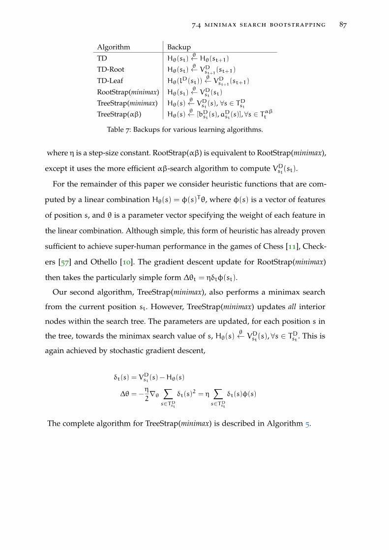
7.4 minimax search bootstrapping 87

Algorithm Backup

TD Hθ(st)θ← Hθ(st+1)

TD-Root Hθ(st)θ← VDst+1(st+1)

TD-Leaf Hθ(lD(st))

θ← VDst+1(st+1)

RootStrap(minimax) Hθ(st)θ← VDst (st)

TreeStrap(minimax) Hθ(s)θ← VDst (s), ∀s ∈ T

Dst

TreeStrap(αβ) Hθ(s)θ← [bDst(s),a

Dst(s)], ∀s ∈ Tαβt

Table 7: Backups for various learning algorithms.

where η is a step-size constant. RootStrap(αβ) is equivalent to RootStrap(minimax),

except it uses the more efficient αβ-search algorithm to compute VDst(st).

For the remainder of this paper we consider heuristic functions that are com-

puted by a linear combination Hθ(s) = φ(s)Tθ, where φ(s) is a vector of features

of position s, and θ is a parameter vector specifying the weight of each feature in

the linear combination. Although simple, this form of heuristic has already proven

sufficient to achieve super-human performance in the games of Chess [11], Check-

ers [57] and Othello [10]. The gradient descent update for RootStrap(minimax)

then takes the particularly simple form ∆θt = ηδtφ(st).

Our second algorithm, TreeStrap(minimax), also performs a minimax search

from the current position st. However, TreeStrap(minimax) updates all interior

nodes within the search tree. The parameters are updated, for each position s in

the tree, towards the minimax search value of s, Hθ(s)θ← VDst(s), ∀s ∈ T

Dst . This is

again achieved by stochastic gradient descent,

δt(s) = VDst(s) −Hθ(s)

∆θ = −η

2∇θ∑s∈TDst

δt(s)2 = η

∑s∈TDst

δt(s)φ(s)

The complete algorithm for TreeStrap(minimax) is described in Algorithm 5.


Algorithm 5 TreeStrap(minimax)

Randomly initialise θInitialise t← 1, s1 ← start statewhile st is not terminal doV ← minimax(st,Hθ,D)for s ∈ search tree doδ← V(s) −Hθ(s)∆θ← ∆θ+ ηδφ(s)

end forθ← θ+∆θSelect at = argmax

a∈AV(st ◦ a)

Execute move at, receive st+1t← t+ 1

end while

Algorithm 6 DeltaFromTransTbl(s,d)

Initialise ∆θ← ~0, t← probe(s)if t is null or depth(t) < d then

return ∆θ

end ifif lowerbound(t) > Hθ(s) then∆θ← ∆θ+ η(lowerbound(t) −Hθ(s))∇Hθ(s)

end ifif upperbound(t) < Hθ(s) then∆θ← ∆θ+ η(upperbound(t) −Hθ(s))∇Hθ(s)

end iffor s ′ ∈ succ(s) do∆θ← DeltaFromTransTbl(s ′)

end forreturn ∆θ

7.5 alpha-beta search bootstrapping

The concept of minimax search bootstrapping can be extended to αβ-search.

Unlike minimax search, alpha-beta does not compute an exact value for the

majority of nodes in the search tree. Instead, the search is cut off when the value

of the node is sufficiently high or low that it can no longer contribute to the

principal variation. We consider a depth D alpha-beta search from root position

7.5 alpha-beta search bootstrapping 89

s0, and denote the upper and lower bounds computed for node s by aDs0(s) and

bDs0(s) respectively, so that bDs0(s) 6 VDs0(s) 6 aDs0(s). Only one bound applies in

cut off nodes: in the case of an alpha-cut we define bDs0(s) to be −∞, and in the

case of a beta-cut we define aDs0(s) to be∞. If no cut off occurs then the bounds

are exact, i.e. aDs0(s) = bDs0(s) = VDs0(s).

The bounded values computed by alpha-beta can be exploited by search boot-

strapping, by using a one-sided loss function. If the value from the heuristic

evaluation is larger than the a-bound of the deep search value, then it is reduced

towards the a-bound, Hθ(s)θ← aDst(s). Similarly, if the value from the heuristic

evaluation is smaller than the b-bound of the deep search value, then it is in-

creased towards the b-bound, Hθ(s)θ← bDst(s). We implement this idea by gradient

descent on the sum of one-sided squared errors:

δat (s) =

aDst(s) −Hθ(s) if Hθ(s) > aDst(s)

0 otherwise

δbt (s) =

bDst(s) −Hθ(s) if Hθ(s) < bDst(s)

0 otherwise

giving

∆θt =η

2∇θ

∑s∈Tαβt

δat (s)2 + δbt (s)

2 = η∑s∈Tαβt

(δat (s) + δ

bt (s)

)φ(s)

where Tαβt is the set of nodes in the alpha-beta search tree at time t. We call this

algorithm TreeStrap(αβ), and note that the update for each node s is equivalent

to the TreeStrap(minimax) update when no cut-off occurs.


7.5.1 Updating Parameters in TreeStrap(αβ)

High performance αβ-search routines rely on transposition tables for move or-

dering, reducing the size of the search space, and for caching previous search

results [58]. A natural way to compute ∆θ for TreeStrap(αβ) from a completed

αβ-search is to recursively step through the transposition table, summing any

relevant bound information. We call this procedure DeltaFromTransTbl, and give

the pseudo-code for it in Algorithm 6.

DeltaFromTransTbl requires a standard transposition table implementation pro-

viding the following routines:

• probe(s), which returns the transposition table entry associated with state s.

• depth(t), which returns the amount of search depth used to determine the

bound estimates stored in transposition table entry t.

• lowerbound(t), which returns the lower bound stored in transposition entry

t.

• upperbound(t), which returns the upper bound stored in transposition

entry t.

In addition, DeltaFromTransTbl requires a parameter d > 1, that limits updates

to ∆θ from transposition table entries based on a minimum of search depth of d.

This can be used to control the number of positions that contribute to ∆θ during

a single update, or limit the computational overhead of the procedure.

7.5.2 The TreeStrap(αβ) algorithm

The TreeStrap(αβ) algorithm can be obtained by two straightforward modifications

to Algorithm 5. First, the call to minimax(st,Hθ,D) must be replaced with a call

7.6 learning chess program 91

to αβ-search(st,Hθ,D). Secondly, the inner loop computing ∆θ is replaced by

invoking DeltaFromTransTbl(st).

7.6 learning chess program

We implemented our learning algorithms in Meep, a modified version of the

tournament chess engine Bodo. For our experiments, the hand-crafted evaluation

function of Bodo was removed and replaced by a weighted linear combination of

1812 features. Given a position s, a feature vector φ(s) can be constructed from the

1812 numeric values of each feature. The majority of these features are binary. φ(s)

is typically sparse, with approximately 100 features active in any given position.

Five well-known, chess specific feature construction concepts: material, piece

square tables, pawn structure, mobility and king safety were used to generate the

1812 distinct features. These features were a strict subset of the features used in

Bodo, which are themselves simplistic compared to a typical tournament engine

[11].

The evaluation function Hθ(s) was a weighted linear combination of the features

i.e.Hθ(s) = φ(s)Tθ. All components of θwere initialised to small random numbers.

Terminal positions were evaluated as −9999.0, 0 and 9999.0 for a loss, draw and

win respectively. In the search tree, mate scores were adjusted inward slightly so

that shorter paths to mate were preferred when giving mate, and vice-versa. When

applying the heuristic evaluation function in the search, the heuristic estimates

were truncated to the interval [−9900.0, 9900.0].

Meep contains two different modes: a tournament mode and a training mode.

When in tournament mode, Meep uses an enhanced alpha-beta based search

algorithm. Tournament mode is used for evaluating the strength of a weight

configuration. In training mode however, one of two different types of game

tree search algorithms are used. The first is a minimax search that stores the


entire game tree in memory. This is used by the TreeStrap(minimax) algorithm.

The second is a generic alpha-beta search implementation, that uses only three

well known alpha-beta search enhancements: transposition tables, killer move

tables and the history heuristic [58]. This simplified search routine was used

by the TreeStrap(αβ) and RootStrap(αβ) algorithms. In addition, to reduce the

horizon effect, checking moves were extended by one ply. During training, the

transposition table was cleared before the search routine was invoked.

Simplified search algorithms were used during training to avoid complicated

interactions with the more advanced heuristic search techniques (such as null

move pruning) useful in tournament play. It must be stressed that during training,

no heuristic or move ordering techniques dependent on knowing properties of

the evaluation weights were used by the search algorithms.

Furthermore, a quiescence search [3] that examined all captures and check

evasions was applied to leaf nodes. This was to improve the stability of the leaf

node evaluations. Again, no knowledge based pruning was performed inside the

quiescence search tree, which meant that the quiescence routine was considerably

slower than in Bodo.

7.7 experimental results

We describe the details of our training procedures, and then proceed to explore the

performance characteristics of our algorithms, RootStrap(αβ), TreeStrap(minimax)

and TreeStrap(αβ) through both a large local tournament and online play. We

present our results in terms of Elo ratings. This is the standard way of quantifying

the strength of a chess player within a pool of players. A 300 to 500 Elo rating

point difference implies a winning rate of about 85% to 95% for the higher rated

player.

7.7 experimental results 93

7.7.0.1 Training Methodology

At the start of each experiment, all weights were initialised to small random values.

Games of self-play were then used to train each player. To maintain diversity

during training, a small opening book was used. Once outside of the opening

book, moves were selected greedily from the results of the search. Each training

game was played within 1m 1s Fischer time controls. That is, both players start

with a minute on the clock, and gain an additional second every time they make

a move. Each training game would last roughly five minutes.

We selected the best step-size for each learning algorithm, from a series of

preliminary experiments: α = 1.0× 10−5 for TD-Leaf and RootStrap(αβ), α =

1.0× 10−6 for TreeStrap(minimax) and 5.0× 10−7 for TreeStrap(αβ). The TreeStrap

variants used a minimum search depth parameter of d = 1. This meant that the

target values were determined by at least one ply of full-width search, plus a

varying amount of quiescence search.

7.7.1 Relative Performance Evaluation

We ran a competition between many different versions of Meep in tournament

mode, each using a heuristic function learned by one of our algorithms. In addition,

a player based on randomly initialised weights was included as a reference, and

arbitrarily assigned an Elo rating of 250. The best ratings achieved by each training

method are displayed in Table 8.

We also measured the performance of each algorithm at intermediate stages

throughout training. Figure 13 shows the performance of each learning algorithm

with increasing numbers of games on a single training run. As each training

game is played using the same time controls, this shows the performance of each

learning algorithm given a fixed amount of computation. Importantly, the time

used for each learning update also took away from the total thinking time.


101

102

103

104

0

500

1000

1500

2000

2500

Number of training games

Rat

ing

(Elo

)

Learning from self−play: Rating versus Number of training games

TreeStrap(alpha−beta)RootStrap(alpha−beta)TreeStrap(minimax)TD−LeafUntrained

Figure 13: Performance when trained via self-play starting from random initial weights.95% confidence intervals are marked at each data point. The x-axis uses alogarithmic scale.

The data shown in Table 8 and Figure 13 was generated by BayesElo, a freely

available program that computes maximum likelihood Elo ratings. In each table,

the estimated Elo rating is given along with a 95% confidence interval. All Elo

values are calculated relative to the reference player, and should not be compared

with Elo ratings of human chess players (including the results of online play,

described in the next section). Approximately 16000 games were played in the

tournament. This took approximately two weeks running in parallel on a 2.4Ghz

quad-core Intel Core 2.

The results demonstrate that learning from many nodes in the search tree is sig-

nificantly more efficient than learning from a single root node. TreeStrap(minimax)

and TreeStrap(αβ) learn effective weights in just a thousand training games and

attain much better maximum performance within the duration of training. In addi-

tion, learning from alpha-beta search is more effective than learning from minimax

search. Alpha-beta search significantly boosts the search depth, by safely pruning

7.7 experimental results 95

Algorithm EloTreeStrap(αβ) 2157± 31TreeStrap(minimax) 1807± 32RootStrap(αβ) 1362± 59TD-Leaf 1068± 36Untrained 250± 63

Table 8: Best performance when trained by self play. 95% confidence intervals given.

away subtrees that cannot affect the minimax value at the root. Although the ma-

jority of nodes now contain one-sided bounds rather than exact values, it appears

that the improvements to the search depth outweigh the loss of bound information.

It does appear however that learning from bound information is less robust, in

the sense that the quality of the weights no longer improves monotonically with

extra training games. More investigation is required to determine whether this

holds in general or whether it is an artifact of our particular experimental setup.

Our results demonstrate that the TreeStrap based algorithms can learn a good

set of weights, starting from random weights, from self-play in the game of chess.

Our experiences using TD-Leaf in this setting were similar to those described in

[2]; within the limits of our training scheme, learning occurred, but only to the

level of weak amateur play. Our results suggest that TreeStrap based methods

are potentially less sensitive to initial starting conditions, and allow for speedier

convergence in self play; it will be interesting to see whether similar results carry

across to domains other than chess.

7.7.2 Evaluation by Internet Play

We also evaluated the performance of the heuristic function learned by

TreeStrap(αβ), by using it in Meep to play against predominantly human op-

position at the Internet Chess Club. We evaluated two heuristic functions, the first


Algorithm Training Partner RatingTreeStrap(αβ) Self Play 1950-2197

TreeStrap(αβ) Shredder 2154-2338

Table 9: Blitz performance at the Internet Chess Club

using weights trained by self-play, and the second using weights trained against

Shredder, a grandmaster strength commercial chess program.

The hardware used online was a 1.8Ghz Opteron, with 256Mb of RAM being

used for the transposition table. Approximately 350K nodes per second were seen

when using the learned evaluation function. A small opening book was used

to make the engine play a variety of different opening lines. Compared to Bodo,

the learned evaluation routine was approximately 3 times slower, even though

the evaluation function contained less features. This was due to a less optimised

implementation, and the heavy use of floating point arithmetic.

Approximately 1000 games were played online, using 3m 3s Fischer time con-

trols, for each heuristic function. Although the heuristic function was fixed, the

online rating fluctuates significantly over time. This is due to the high K factor

used by the Internet Chess Club to update Elo ratings, which is tailored to human

players rather than computer engines.

The online rating of the heuristic learned by self-play corresponds to weak mas-

ter level play. The heuristic learned from games against Shredder were roughly 150

Elo stronger, corresponding to master level performance. Like TD-Leaf, TreeStrap

also benefits from a carefully chosen opponent, though the difference between

self-play and ideal conditions is much less drastic. Furthermore, a total of 13.5/15

points were scored against registered members who had achieved the title of

International Master.

We expect that these results could be further improved by using more powerful

hardware, a more sophisticated evaluation function, or a better opening book.

Furthermore, we used a generic alpha-beta search algorithm for learning. An

7.8 conclusion 97

interesting follow-up would be to explore the interaction between our learning

algorithms and the more exotic alpha-beta search enhancements.

7.8 conclusion

Our main result is demonstrating, for the first time, an algorithm that learns to

play master level Chess entirely through self play, starting from random weights.

To provide insight into the nature of our algorithms, we focused on a single

non-trivial domain. However, the ideas that we have introduced are rather general,

and may have applications beyond deterministic two-player game tree search.

Bootstrapping from search could, in principle, be applied to many other search

algorithms. Simulation-based search algorithms, such as UCT, have outperformed

traditional search algorithms in a number of domains. The TreeStrap algorithm

could be applied, for example, to the heuristic function that is used to initialise

nodes in a UCT search tree with prior knowledge [20]. Alternatively, in stochastic

domains the evaluation function could be updated towards the value of an

expectimax search, or towards the one-sided bounds computed by a *-minimax

search [23, 80]. This approach could be viewed as a generalisation of approximate

dynamic programming, in which the value function is updated from a multi-ply

Bellman backup.

B I B L I O G R A P H Y

[1] Peter Auer. Using confidence bounds for exploitation-exploration trade-offs.

Journal of Machine Learning Research, 3:397–422, 2002.

[2] Jonathan Baxter, Andrew Tridgell, and Lex Weaver. Knightcap: a chess

program that learns by combining td(lambda) with game-tree search. In Proc.

15th International Conf. on Machine Learning, pages 28–36. Morgan Kaufmann,

San Francisco, CA, 1998.

[3] Don F. Beal. A generalised quiescence search algorithm. Artificial Intelligence,

43(1):85–98, 1990.

[4] Don F. Beal and M. C. Smith. Learning piece values using temporal differ-

ences. Journal of the International Computer Chess Association, 1997.

[5] Ron Begleiter, Ran El-Yaniv, and Golan Yona. On prediction using variable

order Markov models. Journal of Artificial Intelligence Research, 22:385–421,

2004.

[6] Dimitri P. Bertsekas and David A. Castanon. Rollout algorithms for stochastic

scheduling problems. Journal of Heuristics, 5(1):89–108, 1999. ISSN 1381-1231.

doi: http://dx.doi.org/10.1023/A:1009634810396.

[7] Hendrik Blockeel and Luc De Raedt. Top-down induction of first-order

logical decision trees. Artificial Intelligence, 101(1-2):285–297, 1998. URL

citeseer.nj.nec.com/blockeel98topdown.html.

[8] Byron Boots, Sajid M. Siddiqi, and Geoffrey J. Gordon. Closing the learning-

planning loop with predictive state representations. In Proceedings of the 9th

99

citeseer.nj.nec.com/blockeel98topdown.html

100 bibliography

International Conference on Autonomous Agents and Multiagent Systems: volume

1 - Volume 1, AAMAS ’10, pages 1369–1370, Richland, SC, 2010. Interna-

tional Foundation for Autonomous Agents and Multiagent Systems. ISBN

978-0-9826571-1-9. URL http://portal.acm.org/citation.cfm?id=1838206.

1838386.

[9] Ronen I. Brafman and Moshe Tennenholtz. R-max - a general polynomial

time algorithm for near-optimal reinforcement learning. Journal of Machine

Learning Research, 3:213–231, 2003. ISSN 1532-4435. doi: http://dx.doi.org/

10.1162/153244303765208377.

[10] M. Buro. From simple features to sophisticated evaluation functions. In First

International Conference on Computers and Games, pages 126–145, 1999.

[11] M. Campbell, A. Hoane, and F. Hsu. Deep Blue. Artificial Intelligence, 134:

57–83, 2002.

[12] Anthony R. Cassandra, Leslie Pack Kaelbling, and Michael L. Littman. Acting

optimally in partially observable stochastic domains. In AAAI, pages 1023–

1028, 1994.

[13] G.M.J-B. Chaslot, M.H.M. Winands, J.W.H.M. Uiterwijk, H.J. van den Herik,

and B. Bouzy. Progressive strategies for Monte-Carlo Tree Search. New

Mathematics and Natural Computation, 4(3):343–357, 2008.

[14] Guillaume M. Chaslot, Mark H. Winands, and H.J. Van den Herik. Parallel

Monte-Carlo Tree Search. In Proceedings of the 6th International Conference on

Computers and Games, pages 60–71, Berlin, Heidelberg, 2008. Springer-Verlag.

ISBN 978-3-540-87607-6. doi: http://dx.doi.org/10.1007/978-3-540-87608-3_

6.

[15] Thomas M. Cover and Joy A. Thomas. Elements of information theory. Wiley-

Interscience, New York, NY, USA, 1991. ISBN 0-471-06259-6.

http://portal.acm.org/citation.cfm?id=1838206.1838386

http://portal.acm.org/citation.cfm?id=1838206.1838386

bibliography 101

[16] Finale Doshi-velez. The Infinite Partially Observable Markov Decision Process.

In Advances in Neural Information Processing Systems, 2009.

[17] V.F. Farias, C.C. Moallemi, B. Van Roy, and T. Weissman. Universal reinforce-

ment learning. Information Theory, IEEE Transactions on, 56(5):2441 –2454, may

2010. ISSN 0018-9448. doi: 10.1109/TIT.2010.2043762.

[18] Hilmar Finnsson and Yngvi Björnsson. Simulation-based approach to general

game playing. In AAAI, pages 259–264, 2008.

[19] Jurgen Van Gael, Yee Whye Teh, and Zoubin Ghahramani. The Infinite

Factorial Hidden Markov Model. In Advances in Neural Information Processing

Systems, 2008.

[20] S. Gelly and D. Silver. Combining online and offline learning in UCT. In

Proceedings of the 17th International Conference on Machine Learning, pages 273–

280, 2007.

[21] Sylvain Gelly and Yizao Wang. Exploration exploitation in Go: UCT for

Monte-Carlo Go. In NIPS Workshop on On-line trading of Exploration and

Exploitation, 2006.

[22] Sylvain Gelly, Yizao Wang, Rémi Munos, and Olivier Teytaud. Modifi-

cation of UCT with patterns in Monte-Carlo Go. Technical Report 6062,

INRIA, France, November 2006. URL http://hal.inria.fr/docs/00/12/

15/16/PDF/RR-6062.pdf.

[23] Thomas Hauk, Michael Buro, and Jonathan Schaeffer. Rediscovering *-

minimax search. In Computers and Games, pages 35–50, 2004.

[24] K.A. Heller, Y.W. Teh, , and D. Gorur. The Infinite Hierarchical Hidden

Markov Model. In AISTATS, 2009.

http://hal.inria.fr/docs/00/12/15/16/PDF/RR-6062.pdf

http://hal.inria.fr/docs/00/12/15/16/PDF/RR-6062.pdf

102 bibliography

[25] Bret Hoehn, Finnegan Southey, Robert C. Holte, and Valeriy Bulitko. Effective

short-term opponent exploitation in simplified poker. In AAAI, pages 783–

788, 2005.

[26] Michael P. Holmes and Charles Lee Isbell Jr. Looping suffix tree-based

inference of partially observable hidden state. In ICML, pages 409–416, 2006.

[27] Marcus Hutter. Self-optimizing and Pareto-optimal policies in general envi-

ronments based on Bayes-mixtures. In Proceedings of the 15th Annual Confer-

ence on Computational Learning Theory (COLT 2002), Lecture Notes in Artificial

Intelligence. Springer, 2002. URL http://www.hutter1.net/ai/selfopt.htm.

[28] Marcus Hutter. The fastest and shortest algorithm for all well-defined prob-

lems. International Journal of Foundations of Computer Science., 13(3):431–443,

2002.

[29] Marcus Hutter. Universal Artificial Intelligence: Sequential Decisions Based on

Algorithmic Probability. Springer, 2005.

[30] Marcus Hutter. Universal algorithmic intelligence: A mathematical

top→down approach. In Artificial General Intelligence, pages 227–290.

Springer, Berlin, 2007. ISBN 3-540-23733-X. URL http://arxiv.org/abs/cs.

AI/0701125.

[31] Leslie Pack Kaelbling, Michael L. Littman, and Anthony R. Cassandra. Plan-

ning and acting in partially observable stochastic domains. Artificial Intelli-

gence, 101:99–134, 1995.

[32] Levente Kocsis and Csaba Szepesvári. Bandit based Monte-Carlo planning.

In ECML, pages 282–293, 2006.

[33] Stefan Kramer and Gerhard Widmer. Inducing classification and regression

trees in first order logic. In Sašo Džeroski and Nada Lavrac, editors, Relational

Data Mining, chapter 6. Springer, 2001.

http://www.hutter1.net/ai/selfopt.htm

http://arxiv.org/abs/cs.AI/0701125

http://arxiv.org/abs/cs.AI/0701125

bibliography 103

[34] R.E. Krichevsky and V.K. Trofimov. The performance of universal coding.

IEEE Transactions on Information Theory, IT-27:199–207, 1981.

[35] H. W. Kuhn. A simplified two-person poker. In Contributions to the Theory of

Games, pages 97–103, 1950.

[36] S. Legg and M. Hutter. Ergodic MDPs admit self-optimising policies. Tech-

nical Report IDSIA-21-04, Dalle Molle Institute for Artificial Intelligence

(IDSIA), 2004.

[37] Shane Legg. Machine Super Intelligence. PhD thesis, Department of Informat-

ics, University of Lugano, 2008.

[38] Leonid A. Levin. Universal sequential search problems. Problems of Informa-

tion Transmission, 9:265–266, 1973.

[39] Ming Li and Paul Vitányi. An Introduction to Kolmogorov Complexity and Its

Applications. Springer, third edition, 2008.

[40] Michael Littman, Richard Sutton, and Satinder Singh. Predictive representa-

tions of state. In NIPS, pages 1555–1561, 2002.

[41] John W. Lloyd. Logic for Learning: Learning Comprehensible Theories from Struc-

tured Data. Springer, 2003.

[42] John W. Lloyd and Kee Siong Ng. Learning modal theories. In Proceedings

of the 16th International Conference on Inductive Logic Programming, LNAI 4455,

pages 320–334, 2007.

[43] Takaki Makino. Proto-predictive representation of states with simple recur-

rent temporal-difference networks. In ICML, pages 697–704, 2009. ISBN

978-1-60558-516-1.

[44] Andrew Kachites McCallum. Reinforcement Learning with Selective Perception

and Hidden State. PhD thesis, University of Rochester, 1996.

104 bibliography

[45] Kee Siong Ng. Learning Comprehensible Theories from Structured Data. PhD

thesis, The Australian National University, 2005.

[46] Sergey Pankov. A computational approximation to the AIXI model. In AGI,

pages 256–267, 2008.

[47] Jan Poland and Marcus Hutter. Defensive universal learning with experts.

In Proc. 16th International Conf. on Algorithmic Learning Theory, volume LNAI

3734, pages 356–370. Springer, 2005.

[48] Jan Poland and Marcus Hutter. Universal learning of repeated matrix games.

Technical Report 18-05, IDSIA, 2006.

[49] Pascal Poupart and Nikos Vlassis. Model-based bayesian reinforcement

learning in partially observable domains. In ISAIM, 2008.

[50] Pascal Poupart, Nikos Vlassis, Jesse Hoey, and Kevin Regan. An analytic

solution to discrete bayesian reinforcement learning. In ICML ’06: Proceedings

of the 23rd international conference on Machine learning, pages 697–704, New

York, NY, USA, 2006. ACM. ISBN 1-59593-383-2. doi: http://doi.acm.org/10.

1145/1143844.1143932.

[51] Martin L. Puterman. Markov Decision Processes: Discrete Stochastic Dynamic

Programming. Wiley-Interscience, 1994.

[52] Jorma Rissanen. A universal data compression system. IEEE Transactions on

Information Theory, 29(5):656–663, 1983.

[53] D. Ron, Y. Singer, and N. Tishby. The power of amnesia: Learning probabilistic

automata with variable memory length. Machine Learning, 25(2):117–150,

1996.

[54] Matthew Rosencrantz, Geoffrey Gordon, and Sebastian Thrun. Learning

low dimensional predictive representations. In Proceedings of the twenty-first

bibliography 105

International Conference on Machine Learning, page 88, New York, NY, USA,

2004. ACM. ISBN 1-58113-828-5. doi: 10.1145/1015330.1015441.

[55] Stephane Ross, Brahim Chaib-draa, and Joelle Pineau. Bayes-adaptive

POMDPs. In J.C. Platt, D. Koller, Y. Singer, and S. Roweis, editors, Advances

in Neural Information Processing Systems 20, pages 1225–1232. MIT Press, Cam-

bridge, MA, 2008.

[56] A L Samuel. Some studies in machine learning using the game of checkers.

IBM Journal of Research and Development, 3, 1959.

[57] J Schaeffer, M Hlynka, and V Jussila. Temporal difference learning applied

to a high performance game playing program. IJCAI, pages 529–534, 2001.

[58] Jonathan Schaeffer. The history heuristic and alpha-beta search enhancements

in practice. IEEE Transactions on Pattern Analysis and Machine Intelligence,

PAMI-11(11):1203–1212, 1989.

[59] J. Schmidhuber, J. Zhao, and M. A. Wiering. Shifting inductive bias

with success-story algorithm, adaptive Levin search, and incremental self-

improvement. Machine Learning, 28:105–130, 1997.

[60] Jürgen Schmidhuber. Discovering neural nets with low Kolmogorov com-

plexity and high generalization capability. Neural Networks, 10(5):857–873,

1997.

[61] Jürgen Schmidhuber. The speed prior: A new simplicity measure yielding

near-optimal computable predictions. In Proc. 15th Annual Conf. on Computa-

tional Learning Theory, pages 216–228, 2002.

[62] Jürgen Schmidhuber. Bias-optimal incremental problem solving. In Advances

in Neural Information Processing Systems 15, pages 1571–1578. MIT Press, 2003.

106 bibliography

[63] Jürgen Schmidhuber. Optimal ordered problem solver. Machine Learning, 54:

211–254, 2004.

[64] Guy Shani. Learning and Solving Partially Observable Markov Decision Processes.

PhD thesis, Ben-Gurion University of the Negev, 2007.

[65] Guy Shani and Ronen Brafman. Resolving perceptual aliasing in the presence

of noisy sensors. In NIPS, 2004.

[66] David Silver and Gerald Tesauro. Monte-carlo simulation balancing. In ICML

’09: Proceedings of the 26th Annual International Conference on Machine Learning,

pages 945–952, New York, NY, USA, 2009. ACM. ISBN 978-1-60558-516-1.

doi: http://doi.acm.org/10.1145/1553374.1553495.

[67] David Silver and Joel Veness. Monte-Carlo Planning in Large POMDPs.

In J. Lafferty, C. K. I. Williams, J. Shawe-Taylor, R.S. Zemel, and A. Culotta,

editors, Advances in Neural Information Processing Systems 23, pages 2164–2172,

2010.

[68] Satinder Singh, Michael James, and Matthew Rudary. Predictive state repre-

sentations: A new theory for modeling dynamical systems. In UAI, pages

512–519, 2004.

[69] Ray J. Solomonoff. A formal theory of inductive inference: Parts 1 and 2.

Information and Control, 7:1–22 and 224–254, 1964.

[70] Alexander L. Strehl, Lihong Li, Eric Wiewiora, John Langford, and Michael L.

Littman. PAC model-free reinforcement learning. In ICML ’06: Proceedings of

the 23rd international conference on Machine learning, pages 881–888, New York,

NY, USA, 2006. ACM. ISBN 1-59593-383-2. doi: http://doi.acm.org/10.1145/

1143844.1143955.

bibliography 107

[71] Alexander L. Strehl, Lihong Li, and Michael L. Littman. Reinforcement

learning in finite MDPs: PAC analysis. Journal of Machine Learning Research,

10:2413–2444, 2009.

[72] M. Strens. A Bayesian framework for reinforcement learning. In ICML, pages

943–950, 2000.

[73] Nobuo Suematsu and Akira Hayashi. A reinforcement learning algorithm in

partially observable environments using short-term memory. In NIPS, pages

1059–1065, 1999.

[74] Nobuo Suematsu, Akira Hayashi, and Shigang Li. A Bayesian approach to

model learning in non-Markovian environment. In ICML, pages 349–357,

1997.

[75] R. Sutton. Learning to predict by the method of temporal differences. Machine

Learning, 3(9):9–44, 1988.

[76] Richard S. Sutton and Andrew G. Barto. Reinforcement Learning: An Introduc-

tion. MIT Press, 1998.

[77] Richard S. Sutton and Brian Tanner. Temporal-difference networks. In NIPS,

2004.

[78] Gerald Tesauro. TD-gammon, a self-teaching backgammon program, achieves

master-level play. Neural Computation, 6(2):215–219, 1994.

[79] Tjalling J. Tjalkens, Yuri M. Shtarkov, and Frans M. J. Willems. Context tree

weighting: Multi-alphabet sources. In Proceedings of the 14th Symposium on

Information Theory Benelux, 1993.

[80] Joel Veness and Alan Blair. Effective use of transposition tables in stochastic

game tree search. In IEEE Symposium on Computational Intelligence and Games,

pages 112–116, 2007.

108 bibliography

[81] Joel Veness, David Silver, William Uther, and Alan Blair. Bootstrapping from

Game Tree Search. In Neural Information Processing Systems (NIPS), 2009.

[82] Joel Veness, Kee Siong Ng, Marcus Hutter, and David Silver. Reinforcement

Learning via AIXI Approximation. In Proceedings of the Conference for the

Association for the Advancement of Artificial Intelligence (AAAI), 2010.

[83] Joel Veness, Kee Siong Ng, Marcus Hutter, William Uther, and David Silver.

A Monte-Carlo AIXI Approximation. Journal of Artificial Intelligence Research

(JAIR), 40(1), 2011.

[84] Tao Wang, Daniel J. Lizotte, Michael H. Bowling, and Dale Schuurmans.

Bayesian sparse sampling for on-line reward optimization. In ICML, pages

956–963, 2005.

[85] Christopher Watkins and Peter Dayan. Q-learning. Machine Learning, 8:

279–292, 1992.

[86] Frans Willems, Yuri Shtarkov, and Tjalling Tjalkens. Reflections on “The

Context Tree Weighting Method: Basic properties”. Newsletter of the IEEE

Information Theory Society, 47(1), 1997.

[87] Frans M. J. Willems. The context-tree weighting method: Extensions. IEEE

Transactions on Information Theory, 44:792–798, 1998.

[88] Frans M. J. Willems, Yuri M. Shtarkov, and Tjalling J. Tjalkens. Context

weighting for general finite-context sources. IEEE Trans. Inform. Theory, 42:

42–1514, 1996.

[89] Frans M.J. Willems, Yuri M. Shtarkov, and Tjalling J. Tjalkens. The context

tree weighting method: Basic properties. IEEE Transactions on Information

Theory, 41:653–664, 1995.

Documents

APPROXIMATE UNIVERSAL ARTIFICIAL Doctor of Philosophy