Embed Size (px)
Citation preview

APPROXIMATE SOLUTIONS OF COUPLED RAMANI
EQUATION BY USING RDTM WITH COMPARED DTM AND
EXACT SOLUTIONS
Murat GUBES1, Galip OTURANC
2
In this paper, we present the new approximate solutions of famous coupled
Ramani Equation. In order to obtain the solution, we use the semi-analytic methods
differential transform method (DTM) and reduced form of DTM called reduced
differential transform method (RDTM). We compare our proposed methods with
exact solution and also compare with together. Numerical results show clearly that
DTM and RDTM are very effective and also provide very accurate solutions.
Additionally, it should be noted that RDTM is applied very easily, fast and more
convergent than DTM for these kind of problems.
Keywords: Reduced differential transform method (RDTM), Differential
transform method (DTM), Coupled Ramani Equation, Approximate solution.
1. Introduction
Partial differential equations are the fundamental phenomena and applied
area in physic, engineering, chemistry and etc. In real life, many events can be
modeled by a nonlinear partial differential equation such as evolution equations.
Particularly in nonlinear sciences, one of the important and outstanding evolution
equation is the famous coupled Ramani Equation that is presented as follow
[1,2,3,4]
2
, 15 , , 15 , ,
45 , , 5 , 18 ,
5 , 3 , , 3 , , 0
, , 3 , , 3 , , 0
xxxxxx xx xxx x xxxx
x xx tt x
xxxt xx t x xt
t xxx x x xx
u x t u x t u x t u x t u x t
u x t u x t u x t v x t
u x t u x t u x t u x t u x t
v x t v x t v x t u x t v x t u x t
(1)
1 Dept.of Mathematics, Karamanoglu Mehmetbey University, Karaman, TURKEY,
e-mail: [email protected] 2 Dept.of Mathematics, Selcuk University, Konya, TURKEY, e-mail:[email protected]

Murat Gubes, Galip Oturanc
In literature, a great number of researchers have studied the system (1) to
obtain exact and approximate solutions as seen some of in [5-16]. Ablowitz and
Clarkson [5], Ito [6], Zhang [7], Feng [8], Malfiet and Hereman [9] have
investigated the solitons and inverse scattering, extensions, exact traveling wave
solutions and traveling solitary wave solutions of nonlinear evolution equations
respectively. Li has presented exact traveling wave solutions of six order Ramani
and a coupled Ramani equation in [10]. In [11], Nadjafikhah and Shirvani-Sh
have found Lie symmetries and conservation laws of Hirota-Ramani equation.
Further, Yusufoğlu and Bekir have obtained the two exact traveling wave
solutions of coupled Ramani equation by applying tanh method as following [12]
0
4 6 2 2 3
4 6 2 2 2
, 2 tanh ,
4 16 5 5,
9 27 9 54
20 16 5tanh
9 9 9
u x t a x t
v x t
x t
(2)
and
0
4 6 2 2 3
4 6 2 2 2
, 2 tan ,
4 16 5 5, ,
9 27 9 54 2
20 16 5tan
9 9 9
u x t a x t
v x t x t
x t
(3)
where 0 , and a are arbitrary constants.
Recently, Wazwaz and Triki [13], Wazwaz [14], Jafarian et all [15] and
Wazwaz [16] have presented the multiple soliton solutions and approximate
solution of eq. (1) respectively.
According to the this, main aim of our study is to obtain accurate,
convergent and efficient approximate solution of coupled Ramani equation (1) by
using differential transform (DTM) and reduced differential transform (RDTM)
methods. For the purpose of efficiency and accuracy, our results are compared
with exact solutions (2)-(3) of eq. (1). Numerical considerations are revealed that
RDTM is very effective and more convergent than DTM. In addition, RDTM can
be applied easier than DTM and ensures very accurate solutions as in tables (3)-
(6) and figures (1)-(4).

Approximate solution of coupled Ramani equation by using RDTM with compared DTM and
exact solutions
2. Basic Properties of Two Dimensional Reduced Differential
Transform Method (RDTM) and Differential Transform Method (DTM)
2.1. Two dimensional DTM
Differential transform method (DTM) is a numerical method based on
Taylor expansion. This method tries to find coefficients of series expansion of
unknown function term by term. The concept of DTM was first proposed by Zhou
[17]. By, considering the literature [17,18,19,20,21,22,23,24], we give the
following definition of two dimensional DTM;
Definition 2.1.: Lets ( , )u x t is denoted two variables analytic and differentiable
function, then two dimensional transform is follow
0
0
1( , ) ( , )
! !
k h
k hx xt t
U k h u x tk h x t
(4)
where ( , )U k h is the transformed function of ( , )u x t . The transformation is called
T-function. Hence, the differential inverse transform of ( , )U k h is defined as
0 0
0 0
( , ) ( , )( ) ( )k h
k h
u x t U k h x x t t
(5)
From the eqs. (4) and (5), it can be written
0
0
0 0
0 0
1( , ) ( , ) ( ) ( )
! !
k hk h
k hx xk ht t
u x t u x t x x t tk h x t
(6)
In terms of applicability, we rearrange the eq. (6) as follow
00 00
1( , ) ( , ) ( , )
! !
k hn mk h
nmk hxk ht
u x t u x t x t R x tk h x t
(7)
where 0 0,x t are taken as 0,0 and

Murat Gubes, Galip Oturanc
1 1
( , ) ( , ) k h
nm
k n h m
R x t U k h x t
(8)
Here, ( , )nmR x t is negligibly small terms. Some of the transform form of functions
are given as Table 1 and their proofs can be found in [17,18,19,20].
Table 1: Some two dimensional DTM operations with transformed forms.
Original functions Transformed forms
( , ) ( , ) ( , )u x t v x t w x t ( , ) ( , ) ( , )U k h V k h W k h
( , ) ( , )u x t v x t ( , ) ( , )U k h V k h
( , ) ( , )u x t v x tx
( , ) ( 1) ( 1, )U k h k V k h
( , ) ( , )u x t v x tt
( , ) ( 1) ( , 1)U k h h V k h
( , ) ( , )m n
m nu x t v x t
x t
( )! ( )!
( , ) ( , )! !
k m h nU k h V k m h n
k h
( , ) ( , ) ( , )u x t v x t w x t 0 0
( , ) ( , ) ( , )k h
r s
U k h V r h s W k r s
( , ) ( , ) ( , ) ( , )u x t v x t w x t q x t 0 0 0 0
( , ) ( , ) ( , ) ( , )k k r h h s
r p s z
U k h V r h s z W p s Q k r p z
( , ) m nu x t x t
( , ) ( , ) ( ) ( )U k h k m h n k m h n
1 , ( )
0 ,
k mk m
otherwise
2.2. Two dimensional RDTM
Reduced differential transform method (RDTM) which has an alternative
approach of problems is presented to overcome the demerit complex calculation,
discretization, linearization or perturbations of well-known numerical and
analytical methods such as Adomian decomposition, Differential transform,
Homotopy perturbation and Variational iteration. RDTM was first introduced by
Keskin and Oturanc [26,27,28,29]. The main advantage of RDTM is providing an
analytic approximation, in many cases exact solutions, in rapidly convergent
sequence with elegantly computed terms [24],[26,27,28,29,30,31]. And also,

Approximate solution of coupled Ramani equation by using RDTM with compared DTM and
exact solutions
unlike the DTM, RDTM is based on the Poisson series coefficients expansion. By
using the literature [24],[26,27,28,29,30,31], we present the RDTM as follow.
Definition 2.2.: Lets ( , )u x t is two variables function and assumed that it can be
demonstrated as a product of two functions which are single variable
( , ) ( ) ( )u x t h x g t . By making use of differential transform properties, ( , )u x t can
be written as
0 0 0
( , ) ( ) ( ) ( )i j k
k
i j k
u x t H i x G j t U x t
(9)
Here ( )kU x is called t dimensional spectrum function of ( , )u x t . If function
( , )u x t is analytic and differentiated continuously with respect to time t and space
x in the domain of interest, than
0
1( ) ( , )
!
k
k k
t t
U x u x tk t
(10)
where ( )kU x is transformed function of ( , )u x t . The differential inverse transform
of ( )kU x is defined as
0
0
( , ) ( )( )k
k
k
u x t U x t t
(11)
Combining (9)-(11), we can write
0
0
0
1( , ) ( , ) ( )
!
kk
kk t t
u x t u x t t tk t
(12)
In real applications, we use the finite series form of (12), therefore we rewrite the
solution as
0
( , ) ( )n
k
n k
k
u x t U x t
(13)
where n is order of approximation. Hence, the RDTM solution is given by

Murat Gubes, Galip Oturanc
( , ) lim ( , )nn
u x t u x t
(14)
here n is taken as sufficiently big to get convergent solution. In Table 2,
transformed form of mathematical operation of some functions are given and their
proofs are shown in ref. [26,27].
3. Solution procedures of Ramani Equation by DTM and RDTM
3.1. DTM procedure Let's consider the coupled Ramani equation (1) with two different initial
conditions as [4],[10],[12,13,14,15,16]
0
4 6 2 2 3
4 6 2 22
( ,0) 2 tanh( )
4 16 5 5( ,0)
9 27 9 54
20 16 5 tanh ( )
9 9 9
u x a x
v x
x
(15)
0
4 6 2 2 3
4 6 2 22
( ,0) 2 tan( )
4 16 5 5( ,0)
9 27 9 54
20 16 5 tan ( )
9 9 9
u x a x
v x
x
(16)
( , ), ( , )U k h V k h , which are called T-function, denote the transformation of the
functions ( , ), ( , )u x t v x t in eq. (1) respectively. Then from Table 1 and (4) to (7),
we obtain the transformed form of eq. (1) as below
0 0
( 6)!5( 1)( 2) ( , 2) ( 6, ) 18( 1) ( 1, )
!
1 4 1 2 315
1, 4,
k h
r s
kh h U k h U k h k V k h
k
r k r k r k r k r
U r h s U k r s
(17)

Approximate solution of coupled Ramani equation by using RDTM with compared DTM and
exact solutions
0 0
0 0
0 0
1 2 1 2 3 2,15
3,
3 !5 1 ( 3, 1)
!
1 1 2 2,15
, 1
15 1 1 1 1, 1, 1
1 1 1 245
1, 1,
k h
r s
k h
r s
k h
r s
r r k r k r k r U r h s
U k r s
kh U k h
k
h s k r k r U k r s
U r h s
r k r h s U r h s U k r h s
r l k r l k r l
U r h s p U l s
0 0 0 0 2,
k k r h h s
r l s p U k r l p
0 0
0 0
( 3)!( 1) ( , 1) ( 3, )
!
1 1 1,3
1,
1 2 ,3
2,
k h
r s
k h
r s
kh V k h V k h
k
r k r V r h s
U k r s
k r k r V r h s
U k r s
(18)
and for initial conditions (15-16), we obtain as
0
4 6 2 2 3
24 6 2 2
2 ! ( ,0)( ,0) ( ,0) 2
2 ! ( ,0)
4 16 5 5( ,0) ( ,0)
9 27 9 54
2 ! ( ,0)20 16 5 +
9 9 9 2 ! ( ,0)
k
k
k
k
k kU k a k
k k
V k k
k k
k k
(19)
and
0( ,0) ( ,0) 2 tan2
kU k a k
Murat Gubes, Galip Oturanc
4 6 2 2 34 16 5 5( ,0) ( ,0)
9 27 9 54V k k
(20)
24 6 2 220 16 5 + tan
9 9 9 2
k
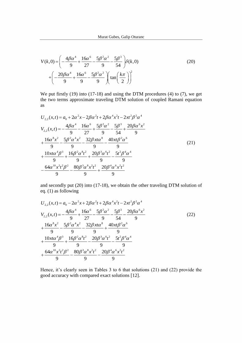
We put firstly (19) into (17-18) and using the DTM procedures (4) to (7), we get
the two terms approximate traveling DTM solution of coupled Ramani equation
as
2 2 4 2 2 2 4
2,2 0
4 6 2 2 3 6 2
2,2
8 2 2 4 2 8 2 6
4 3 2 8 2 3 6 2 2 4 4
10 2 2 2 3 8 2 2 4 6 2 2
( , ) 2 2 2 2
4 16 5 5 20( , )
9 27 9 54 9
16 5 32 40
9 9 9 9
10 16 20 5
9 9 9 9
64 80 20
9 9 9
U x t a x t x t xt
xV x t
x x xt xt
xt t t t
x t x t x t
(21)
and secondly put (20) into (17-18), we obtain the other traveling DTM solution of
eq. (1) as following
2 2 4 2 2 2 4
2,2 0( , ) 2 2 2 2U x t a x t x t xt
4 6 2 2 3 6 2
2,2
4 16 5 5 20( , )
9 27 9 54 9
xV x t
(22)
8 2 2 4 2 8 2 616 5 32 40
9 9 9 9
x x xt xt
4 3 2 8 2 3 6 2 2 4 410 16 20 5
9 9 9 9
xt t t t
10 2 2 2 3 8 2 2 4 6 2 264 80 20
9 9 9
x t x t x t
Hence, it’s clearly seen in Tables 3 to 6 that solutions (21) and (22) provide the
good accuracy with compared exact solutions [12].

Approximate solution of coupled Ramani equation by using RDTM with compared DTM and
exact solutions
3.1. RDTM procedure
As the same manner, again we consider the eq. (1) with initial conditions (15-16)
to obtain the RDTM solutions. ( ), ( )k kU x V x , which are called t dimensional
spectrum functions, denote the transformation of the functions ( , ), ( , )u x t v x t in
eq. (1) respectively. Then from Table 2 and (9) to (14), we obtain the transformed
form of eq. (1) as below
6
2 6
2 3 4
2 3 40 0
2
20 0
3 2
1 13 20
5( 1)( 2) ( ) ( ) 18 ( )
15 ( ) ( ) 15 ( ) ( )
45 ( ) ( ) ( )
5( 1) ( ) 15 ( )( 1) ( )
15
k k k
k k
k r r k r r
r r
k k r
r s k r s
r s
k
k r k r
r
d dk k U x U x V x
dx dx
d d d dU x U x U x U x
dx dx dx dx
d d dU x U x U x
dx dx dx
d dk U x U x k r U x
dx dx
d
1
0
( )( 1) ( )k
r k r
r
dU x k r U x
dx dx
(23)
3
1 3
2
20 0
( 1) ( ) ( )
3 ( ) ( ) 3 ( ) ( )
k k
k k
r k r r k r
r r
dk V x V x
dx
d d dV x U x V x U x
dx dx dx
(24)
and for initial conditions (15-16), we obtain reduced transform form as
respectively
0 0( ) 2 tanhU x a x
4 6 2 2 3
0
4 6 2 22
4 16 5 5( )
9 27 9 54
20 16 5 + tanh
9 9 9
V x
x
(25)
and

Murat Gubes, Galip Oturanc
0 0( ) 2 tanU x a x
4 6 2 2 3
0
4 16 5 5( )
9 27 9 54V x
(26)
4 6 2 2
220 16 5 + tan
9 9 9x
Table 2: Some two dimensional RDTM operations with transformed forms.
Original functions Transformed forms
( , ) ( , ) ( , )u x t v x t w x t ( ) ( ) ( )k k kU x V x W x
( , ) ( , )u x t v x t ( ) ( ) , is constantk kU x V x
( , ) ( , )u x t v x tx
( ) ( )k kU x V x
( , ) ( , )r
ru x t v x t
t
( )!
( ) ( )!
k k r
k rU x V x
k
( , ) ( , ) ( , )u x t v x t w x t 0 0
( ) ( ) ( ) ( ) ( )k k
k r k r r k r
r r
U x V x W x W x V x
( , ) ( , ) ( , ) ( , )u x t v x t w x t q x t 0 0
( ) ( ) ( ) ( )k k r
k r p k r p
r p
U x V x W x Q x
( , ) m nu x t x t ,
( ) ( ) , ( )0 , otherwise
m
m
k
x k nU x x k n k n
As in the DTM solution process, by using RDTM algorithm we put firstly (25)
into (23-24), we get the two terms RDTM solution of coupled Ramani equation as
7 6
0
5 22 7 2
2 7 22 7 2 5
42 3 2
cosh 2 sinh cosh
2 cosh 96 sinh cosh1( )
cosh 144 sinh 24 sinh cosh
2 sinh cosh
a x x x
t x t x xU x
x t x t x x
t x x
(27)
2 10 2 8 2
2 8 4 8 2 12
302400 756001( )
54cosh( ) 96 cosh( ) 241920
t tV x
x x t
(28)

Approximate solution of coupled Ramani equation by using RDTM with compared DTM and
exact solutions
6 8 3 8
7 5
7 3
5 2 5
5 2 3
2 10 6 4
82 10 2
64 cosh( ) 5 cosh( )
960 sinh( )cosh( )
2880 sinh( )cosh( )
240 sinh( )cosh( )
720 sinh( )cosh( )
3840cosh( ) 120960cosh( )1
54cosh( ) 403200 cosh( )
x x
t x x
t x x
t x x
t x x
t x x
x t x
2 8 2 6
2 8 2 4 2 8 2 2
4 6 2 2 6
12 2 6 12 2 4
12 2 2 9 5
9 3
960 cosh( )
30240 cosh( ) 100800 cosh( )
120 cosh( ) 30 cosh( )
3072 cosh( ) 96768 cosh( )
322560 cosh( ) 768 cosh( ) sinh( )
2304 cosh( ) sinh(
t x
t x t x
x x
t x t x
t x t x x
t x
6 6) 96 cosh( )x x
and secondly put (26) into (23-24), we obtain the other RDTM solution of eq. (1)
as following
7 6
0
5 22 7 2
2 7 22 7 2 5
42 3 2
cos 2 sin cos
2 cos 96 sin cos1( )
cosh 144 sin 24 sin cos
2 sin cos
a x x x
t x t x xU x
x t x t x x
t x x
(29)
2 10 2 8 2
4 8 2 12
6 8 3 8
7 5
7 3
2 8
5 2 5
5 2 3
2 10
302400 75600
96 cos( ) 241920
64 cos( ) 5 cos( )
960 sin( )cos( )1
( ) 2880 sin( )cos( )54cosh( )
240 sin( )cos( )
720 sin( )cos( )
3840
t t
x t
x x
t x x
V x t x xx
t x x
t x x
t
6 4
4 6 2 2 6
cos( ) 120960cos( )
120 cos( ) 30 cos( )
x x
x x
(30)

Murat Gubes, Galip Oturanc
2 10 2 2 8 2 6
2 8 2 4 2 8 2 2
12 2 2 9 5
8
12 2 6 12 2 4
9 3 6
403200 cos( ) 960 cos( )
30240 cos( ) 100800 cos( )1
322560 cos( ) 768 cos( ) sin( )54cosh( )
3072 cos( ) 96768 cos( )
2304 cos( ) sin( ) 96
t x t x
t x t x
t x t x xx
t x t x
t x x
6cos( )x
Thus, it’s obviously noted on the Tables 3 to 6 and Figures 1 to 4 that solutions
(29) and (30) provide the good accuracy with compared exact [12] and DTM
solutions.
Table 3: The numerical results of three terms DTM and RDTM solutions of eq. (1) with compared
exact solution (2) at 020 and 1, 0.01t a
x Exact [12]
( , )u x t
RDTM
3( )U x
DTM
3,3( , )U x t
Exact [12]
( , )v x t
RDTM
3( )V x
DTM
3,3( , )V x t
-50 0.990726228 0.9907262253 0.9908033667 -8.822839648×10⁻⁸
-8.822106112×10⁻⁸
-8.842207168×10⁻⁸
-40 0.9923668212 0.9923668187 0.9923930999 -8.785868735×10⁻⁸
-8.785217835×10⁻⁸
-8.794184127×10⁻⁸
-30 0.9941371636 0.9941371613 0.9941436287 -8.754022597×10⁻⁸
-8.753492301×10⁻⁸
-8.756755781×10⁻⁸
-20 0.9960140671 0.9960140653 0.9960149542 -8.729383894×10⁻⁸
-8.729008043×10⁻⁸
-8.729939194×10⁻⁸
-10 0.9979670454 0.9979670444 0.9979670778 -8.713716109×10⁻⁸
-8.713520228×10⁻⁸
-8.712751428×10⁻⁸
10 1.001953749 1.001953750 1.001953722 -8.713295226×10⁻⁸
-8.713487060×10⁻⁸
-8.713330592×10⁻⁸
20 1.003909050 1.003909050 1.003908246 -8.72857484×10⁻⁸
-8.728947099×10⁻⁸
-8.729131646×10⁻⁸
30 1.005789625 1.005789629 1.005783571 -8.752885527×10⁻⁸
-8.753412915×10⁻⁸
-8.755629763×10⁻⁸
40 1.007564728 1.007564730 1.0075397 -8.784482114×10⁻⁸
-8.785130927×10⁻⁸
-8.792842001×10⁻⁸
50 1.009210856 1.009210859 1.009136633 -8.821289529×10⁻⁸
-8.822021826×10⁻⁸
-8.840785424×10⁻⁸
4. Results and Conclusions
In this paper, we consider the very famous physical problems coupled
Ramani equation (1) to find two approximate traveling wave solutions by using
DTM and RDTM. Moreover, we perfectly obtain approximate solutions of (1)
compatible with exact solutions in [12]. In order to test efficiency, convergence
and accuracy of DTM and RDTM, we perform the numerical values
0 1, 0.01, 0.01a in the three term approximate solutions of eq. (1) which
are shown in Tables 3 to 6. Also, for 0
1, 0.03, 0.03
2a and
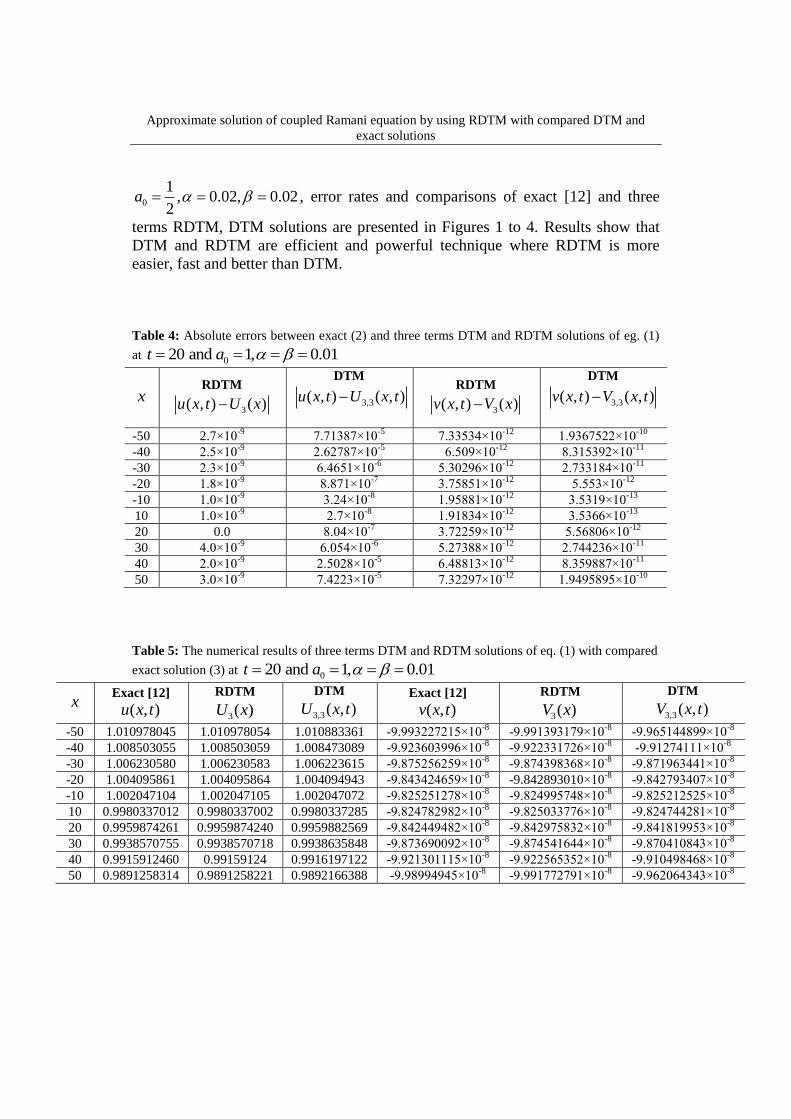
Approximate solution of coupled Ramani equation by using RDTM with compared DTM and
exact solutions
0
1, 0.02, 0.02
2a , error rates and comparisons of exact [12] and three
terms RDTM, DTM solutions are presented in Figures 1 to 4. Results show that
DTM and RDTM are efficient and powerful technique where RDTM is more
easier, fast and better than DTM.
Table 4: Absolute errors between exact (2) and three terms DTM and RDTM solutions of eg. (1)
at 020 and 1, 0.01t a
x RDTM
3( , ) ( )u x t U x
DTM
3,3( , ) ( , )u x t U x t
RDTM
3( , ) ( )v x t V x
DTM
3,3( , ) ( , )v x t V x t
-50 2.7×10⁻⁹
7.71387×10⁻⁵
7.33534×10⁻¹²
1.9367522×10⁻¹⁰
-40 2.5×10⁻⁹
2.62787×10⁻⁵
6.509×10⁻¹²
8.315392×10⁻¹¹
-30 2.3×10⁻⁹
6.4651×10⁻⁶
5.30296×10⁻¹²
2.733184×10⁻¹¹
-20 1.8×10⁻⁹
8.871×10⁻⁷
3.75851×10⁻¹²
5.553×10⁻¹²
-10 1.0×10⁻⁹
3.24×10⁻⁸
1.95881×10⁻¹²
3.5319×10⁻¹³
10 1.0×10⁻⁹
2.7×10⁻⁸
1.91834×10⁻¹²
3.5366×10⁻¹³
20 0.0 8.04×10⁻⁷
3.72259×10⁻¹²
5.56806×10⁻¹²
30 4.0×10⁻⁹
6.054×10⁻⁶
5.27388×10⁻¹²
2.744236×10⁻¹¹
40 2.0×10⁻⁹
2.5028×10⁻⁵
6.48813×10⁻¹²
8.359887×10⁻¹¹
50 3.0×10⁻⁹
7.4223×10⁻⁵
7.32297×10⁻¹²
1.9495895×10⁻¹⁰
Table 5: The numerical results of three terms DTM and RDTM solutions of eq. (1) with compared
exact solution (3) at 020 and 1, 0.01t a
x Exact [12]
( , )u x t
RDTM
3( )U x
DTM
3,3( , )U x t
Exact [12]
( , )v x t
RDTM
3( )V x
DTM
3,3( , )V x t
-50 1.010978045 1.010978054 1.010883361 -9.993227215×10⁻⁸
-9.991393179×10⁻⁸
-9.965144899×10⁻⁸
-40 1.008503055 1.008503059 1.008473089 -9.923603996×10⁻⁸
-9.922331726×10⁻⁸
-9.91274111×10⁻⁸
-30 1.006230580 1.006230583 1.006223615 -9.875256259×10⁻⁸
-9.874398368×10⁻⁸
-9.871963441×10⁻⁸
-20 1.004095861 1.004095864 1.004094943 -9.843424659×10⁻⁸
-9.842893010×10⁻⁸
-9.842793407×10⁻⁸
-10 1.002047104 1.002047105 1.002047072 -9.825251278×10⁻⁸
-9.824995748×10⁻⁸
-9.825212525×10⁻⁸
10 0.9980337012 0.9980337002 0.9980337285 -9.824782982×10⁻⁸
-9.825033776×10⁻⁸
-9.824744281×10⁻⁸
20 0.9959874261 0.9959874240 0.9959882569 -9.842449482×10⁻⁸
-9.842975832×10⁻⁸
-9.841819953×10⁻⁸
30 0.9938570755 0.9938570718 0.9938635848 -9.873690092×10⁻⁸
-9.874541644×10⁻⁸
-9.870410843×10⁻⁸
40 0.9915912460 0.99159124 0.9916197122 -9.921301115×10⁻⁸
-9.922565352×10⁻⁸
-9.910498468×10⁻⁸
50 0.9891258314 0.9891258221 0.9892166388 -9.98994945×10⁻⁸
-9.991772791×10⁻⁸
-9.962064343×10⁻⁸

Murat Gubes, Galip Oturanc
Table 6: Absolute errors between exact (3) and three terms DTM and RDTM solutions of eg. (1)
at 020 and 1, 0.01t a
x RDTM
3( , ) ( )u x t U x
DTM
3,3( , ) ( , )u x t U x t
RDTM
3( , ) ( )v x t V x
DTM
3,3( , ) ( , )v x t V x t
-50 9.0×10⁻⁹
9.4684×10⁻⁵
1.834036×10⁻¹¹
2.8082316×10⁻¹⁰
-40 4.0×10⁻⁹
2.9966×10⁻⁵
1.272270×10⁻¹¹
1.0862886×10⁻¹⁰
-30 3.0×10⁻⁹
6.965×10⁻⁶
8.57891×10⁻¹²
3.292818×10⁻¹¹
-20 3.0×10⁻⁹
9.18×10⁻⁷
5.31649×10⁻¹²
6.31252×10⁻¹²
-10 1.0×10⁻⁹
3.2×10⁻⁸
2.55530×10⁻¹²
3.8753×10⁻¹³
10 1.0×10⁻⁹
2.73×10⁻⁸
2.50794×10⁻¹²
3.8701×10⁻¹³
20 2.1×10⁻⁹
8.308×10⁻⁷
5.2635×10⁻¹²
6.29529×10⁻¹²
30 3.7×10⁻⁹
6.5093×10⁻⁶
8.51552×10⁻¹²
3.279249×10⁻¹¹
40 6.0×10⁻⁹
2.84662×10⁻⁵
1.264237×10⁻¹¹
1.0802647×10⁻¹⁰
50 9.3×10⁻⁹
9.08074×10⁻⁵
1.823341×10⁻¹¹
2.7885107×10⁻¹⁰
R E F E R E N C E S
[1] Ramani A., Inverse scattering, ordinary differential equations of Painleve-type and Hirota’s
bilinear formalism. In: Fourth International Conference Collective Phenomena, New York:
Academy of Sciences (1981), p. 54.
[2] Hirota R., Direct method of finding exact solutions of nonlinear evolution equations, In:
Bullough R., Caudrey P., editors. Backlund transformations, Berlin, Springer (1980), p. 1157-75.
[3] Hu X. B., Wang D. L., Tam H. W., Lax pairs and backlund transformations for a coupled
Ramani equation and its related system, Applied Mathematics Letters (2000), 13, 45-48.
[4] Zhao J. X., Tam H. W., Soliton solutions of a coupled Ramani equation, Appl Math Lett, 16
(2006), 307-313.
[5] Ablowitz M. J., Clarkson P. A., Solitons, nonlinear evolution equations and inverse scattering
transform, Cambridge University press, 1990.
[6] Ito M., An extension of nonlinear evolution equations K-dV (mK-dV) type to higher order, J.
Physc. Soc. Jpn. (1980), 49 (2), 771-778.
[7] Zhang H., New exact traveling wave solutions for some nonlinear evolution equations, Chaos
Solitons and Fractals (2005), 26 (3), 921-5.
[8] Feng Z., Traveling solitary wave solutions to evolution equations with nonlinear terms any
order, Chaos Solitons and Fractals (2003), 17 (5), 861-8.
[9] Malfliet W., Hereman W., The tanh method: I Exact solutions of nonlinear evolution and wave
equations, Physica Sprica (1996), 54, 569-75.
[10] Li J., Existence of exact families of traveling wave solutions for the sixth-order Ramani
equation and a coupled Ramani equation, Int. J. Bifurc. Chaos (2012), 22 (1), 125002.
[11] Nadjafikhah M., Shirvani-Sh V., Lie symmetries and conservation laws of the Hirota-Ramani
equation, Commun. Nonlin. Sci. Numer. Simul. (2012), 17 (11), 4064-4073.
[12] Yusufoglu E., Bekir A., Exact solutions of coupled nonlinear evolution equations, Chaos
Solitons and Fractals (2008), 37, 842-848.

Approximate solution of coupled Ramani equation by using RDTM with compared DTM and
exact solutions
[13] Wazwaz A. M., Triki H., Multiple soliton solutions for the sixth-order Ramani equation and a
coupled Ramani equation, Applied Mathematics and Computation (2010), 216, 332-336.
[14] Wazwaz A. M., A coupled Ramani equation: multiple soliton solutions, J. Math. Chem.
(2014), 52, 2133-2140.
[15] Jafarian A., Ghaderi P., Golmankaneh A. K., Baleanu D., Homotopy analysis method for
solving coupled Ramani Equations, Rom. Journ. Phys. (2014), 59 (1-2), 26-35.
[16] Wazwaz A. M., Multiple soliton solutions for a new coupled Ramani equation, Physica
Scripta (2011), 83, 015002.
[17] Zhou J. K., Differential Transformation and its Applications for Electrical Circuits. Huarjung
University Press, Wuuhahn, China, (1986).
[18] Jang M. J., Chen C. L., Liu Y. C., On solving the initial value problem using the differential
transformation method, Applied Mathematics and Computation (2000), 115, 145-160.
[19] Chen C. L., Ho S. H., Application of differential transformation to eigenvalue problems,
Applied Mathematics and Computation (1996), 79, 173-188.
[20] Kurnaz A., Oturanç G., Kiris M.E., N-Dimensional differential transformation method for
solving PDEs, International Journal of Computer Mathematics (2005), 82(3), 369-380.
[21] Kurnaz A, Oturanc G., The differential transform approximation for the system of ordinary
differential equations, Int J. Comput. Math. (2005), 82,709–719.
[22] Keskin Y., Kurnaz A., Kiris M. E., Oturanc G., Approximate solutions of generalized
pantograph equations by the differential transform method. International Journal of Nonlinear
Sciences and Numerical Simulation (2011), 8(2), 159-164.
[23] Gubes M., Peker H. A., Oturanc G., Application of Differential transform method for El Nino
Southern oscillation (ENSO) model with compared Adomian decomposition and variational
iteration methods, J. Math. & Comput. Sci. (2015), 15, 167-178.
[24] Abazari R., Abazari M., Numerical simulation of generalized Hirota-Satsuma coupled KdV
equation by RDTM and comparison with DTM, Commun. Nonlin. Sci. Numer. Simul. (2012), 17,
619-629.
[25] Abazari R., Borhanifar A., Numerical study of Burgers and coupled Burgers equations by
differential transformation method, Comput Math Appl (2010), 59, 2711–2722.
[26] Keskin Y., Oturanc G, Reduced Differential Transform Method for Partial Differential
Equations, Int. J. Nonlinear Sci. and Num. Simulat. (2009), 10(6), 741-749.
[27] Keskin Y., PhD thesis, Selcuk University, 2010 (in Turkish).
[28] Keskin Y., Oturanc G, Reduced Differential Transform Method for Solving Linear and
Nonlinear Wave Equations, Iranian Journal of Science and Technology (2010), Trans A 34, A2.
[29] Keskin Y., Oturanc G., Reduced Differential Transform Method for fractional partial
differential equations, Nonlinear Science Letters A (2010),1(2), 61-72.
[30] Rawashdeh M. S., An Efficient Approach for Time-Fractional Damped Burger and Time-
Sharma-Tasso-Olver Equations Using the FRDTM, Appl. Math. Inf. Sci. (2015), 9(3), 1239-1246.
[31] Rawashdeh M. S., Obeidat N. A., On Finding Exact and Approximate Solutions to Some
PDEs Using the Reduced Differential Transform Method, Appl. Math. Inf. Sci. (2014), 8(5), 2171-
2176.
Murat Gubes, Galip Oturanc
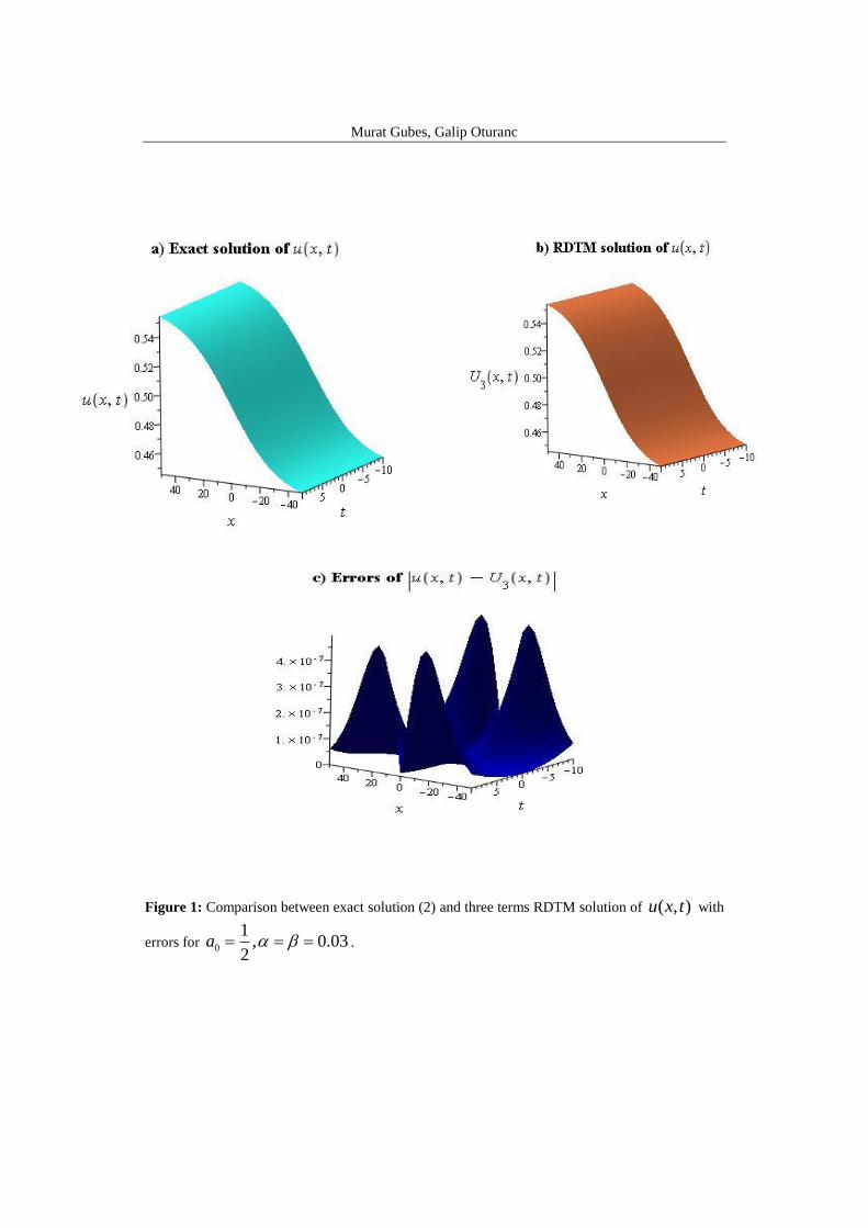
Figure 1: Comparison between exact solution (2) and three terms RDTM solution of ( , )u x t with
errors for 0
1, 0.03
2a .

Approximate solution of coupled Ramani equation by using RDTM with compared DTM and
exact solutions
Figure 2: Comparison between exact solution (2) and three terms RDTM solution of ( , )v x t with
errors for 0
1, 0.03
2a .
Murat Gubes, Galip Oturanc
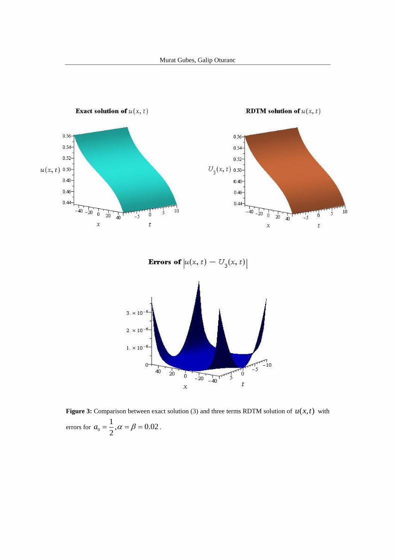
Figure 3: Comparison between exact solution (3) and three terms RDTM solution of ( , )u x t with
errors for 0
1, 0.02
2a .

Approximate solution of coupled Ramani equation by using RDTM with compared DTM and
exact solutions
Figure 4: Comparison between exact solution (3) and three terms RDTM solution of ( , )v x t with
errors for 0
1, 0.02
2a .