Punjab UniversityJournal of Mathematics (ISSN 1016-2526) Vol. 51(2)(2019) pp. 145-158

Approximate Solutions of Ginzburg-Landau Equation using Two Reliable Techniques

Nauman RazaDepartment of Mathematics,

University of the Punjab, Lahore, Pakistan,Email: nauman.math@pu.edu.pk

Received: 07 June, 2018 / Accepted: 01 August, 2018 / Published online: 22 Decemberber, 2018

Abstract. The aim of this article is to compare the Sobolev gradient tech-nique with the Adomian decomposition method for computing a Ginzburg-Landau equation. A convergence criterion for the application of ADM tothe generalized Ginzburg-Landau equation is also presented. From thecomputational point of view, the Sobolev gradient is efficient, easy to useand offer greater accuracy in case of larger domains than ADM.

AMS (MOS) Subject Classification Codes: 35K60; 46C05Key Words:Sobolev gradients; Steepest descent method, Ginzburg-Landau equation.

1. INTRODUCTION

A number of real life problems are modeled as nonlinear differential equations which are not easy to handle due to the difficulties in solving them either analytically or numer-ically. We encounter such problems in many branches of science and engineering. While solving these problems, we have to make certain assumptions to solve them. The traditional methods usually need linearization, discretization, perturbation or some transformations in order to solve nonlinear systems.These methods include Adomian decomposition method, introduced by Adomian [2, 3] which provides a quickly convergent series solution and needs no such alterations. Other methods include homotopy decomposition method, Taylor collocation method, differential transform method, homotopy perturbation method, variational iteration method [5, 6, 9, 16, 18, 19, 7, 10, 11, 29] and many more [12, 13, 14, 23, 30, 33, 37]. These methods has success to deal with nonlinear problems, but the region of convergence is not up to the desired solution. To overcome these drawbacks, research has been carried to derive new algorithms based on the gradient techniques.For the solution of PDEs, it is convenient to construct a functional which represent the sum of square of residues of the equation to be solved and to find the critical point of that functional. The points at which the functional is minimal are the solutions of the given differential equation. This is the basis of steepest descent methods. This method always

145

146 Nauman Raza

gives the minimum of the functional. However, the biggest disadvantage of the method isthat, if it is used on a badly scaled system to locate the minimum, it will take an infinitenumber of iterations. The convergence speed is slow since each step taken towards a min-imum is very small. If we take larger steps then the result obtained may have large errors.To overcome this problem, the recently developed theory of Sobolev gradients [27] gives asystematic way to deal such problems, both in function spaces and finite dimensional set-tings. Sobolev gradients have been successfully applied for the solution of ODEs [27, 25]and PDEs [25, 8].

The method has also been used to find minima of energy functionals. Sial et. al. mini-mized energy functionals related with GL models [34, 35, 36] and their corresponding timeevolution is discussed in [31, 32]. Karotson used this method as a preconditioner for non-linear elliptic problems [22], for the potential equation in electrostatic [20] and semilinearelliptic systems [21]. Knowles used it to solve some inverse problems in groundwater mod-eling [15] and in elasticity [24]. Nattika and Sauter [28] applied this method successfullyto solve differential algebraic equations.Many researchers have compared the ADM with other existing methods to solve stochasticand deterministic problems. Edwerd et. al. [17] have compared the ADM and RK meth-ods to approximate solutions of predator prey model equations. Wazwaz [38] showed acomparison between ADM and Taylor series methods. In this paper the aim is to compareADM with some gradient descent methods such as Sobolev gradient method. The solutionof the Ginzburg-Landau (GL) equation using ADM has already been provided by Adomian[4] but no convergence analysis of the proposed method is discussed. So, one of our contri-bution in this article is to furnish that the sufficient condition of convergence for the seriessolution obtained.The paper is organized as follow, in section2, the proposed model is presented, section3deals with the ADM applied to G-L equation, in section4, convergence proof in case ofreal G-L equation is discussed. Next we apply the Sobolev gradient method on the givenmodel problem. In the subsequent section, numerical results are presented by solving anexample and in the end, the summary of the results obtained is discussed.

2. A MODEL PROBLEM

Consider the GL equation

∂p

∂t= γp− (k + ic) | p |2 p + (µ + ib)

∂2p

∂x2, (2. 1)

with corresponding initial condition

p(x, 0) = g(x), 0 ≤ x ≤ 1, t > 0

whereb, c, k, µ andγ are real,µ > 0, k > 0. Takingb, c = 0, we get the real GL equation

∂p

∂t= γp− k | p |2 p + µ

∂2p

∂x2. (2. 2)

ApproximateSolutionsof Ginzburg-Landau Equation using Two Reliable Techniques 147

The aim of this research is to furnish the condition which is sufficient for the convergenceof the GL equation in real case.

3. ADOMIAN DECOMPOSITIONMETHOD (ADM)

To solve Eq. ( 2. 1 ) using ADM we define two operators such that

Lt ≡ ∂

∂tand Lx ≡ ∂2

∂x2.

Writing the given equation in operator form

Ltp = (µ + ib)Lxp− (k + ic) | p |2 p + γp. (3. 3)

Lt is an invertible operator andL−1t represents one-fold integration such that,L−1

t (·) =t∫0

(·)dt.

By applyingL−1t on both side of Eq. ( 3. 3 ), we have

L−1t Ltp = L−1

t γp− (k + ic)L−1t | p |2 p + (µ + ib)L−1

t Lxp, (3. 4)

p(x, t)− p(x, 0) = γL−1t p− (k + ic)L−1

t | p |2 p + (µ + ib)L−1t Lxp. (3. 5)

p(x, t) = g(x) + γL−1t p− (k + ic)L−1

t | p |2 p + (µ + ib)L−1t Lxp. (3. 6)

p(x, t) can be written in decomposition form as

p(x, t) =∞∑

n=0

pn(x, t). (3. 7)

Putting Eq. ( 3. 7 ) in Eq. ( 3. 6 ), we get

p(x, t) = g(x) + γL−1t (

∞∑n=0

pn)− (k + ic)L−1t (

∞∑n=0

An{| p |2 p})

+(µ + ib)L−1t Lx(

∞∑n=0

pn). (3. 8)

p0 = g(x) = p(x, 0), (3. 9)

p1 = γL−1t p0 − (k + ic)L−1

t (A0) + (µ + ib)L−1t Lxp0, (3. 10)

p2 = γL−1t p1 − (k + ic)L−1

t (A1) + (µ + ib)L−1t Lxp1, (3. 11)

......

148 Nauman Raza

pn+1 = γL−1t pn − (k + ic)L−1

t (An) + (µ + ib)L−1t Lxpn. (3. 12)

whereAn are the Adomian polynomials which need to be evaluated, and anm-term ap-

proximant to evaluatep is φm =m∑

n=0pn that converges top.

Now to evaluateA{| p |2}, we introduce the following functions

| p |= pη(p); η(p) = H(u)− H(−u),

whereH andη are the Heaviside step functions of first and second kind respectively. Thefunctions are defined as below

H = +1, for p > 0 and0 for p < 0,

andη = +1, for p > 0 and−1 for p < 0.

Therefore,| p |2 p = p3η2(p).

Now we findA{| p |2 p}

A0 = p30,

A1 = 3p20p1,

A2 = 3p20p2 + 3p2

1p0,

A3 = p31 + 3p2

0p3 + 6p0p1p2,

A4 = 3p20p4 + 3p2

1p2 + 3p22p0 + 6p0p1p3,

A5 = 3p20p5 + 3p2

1p3 + 3p22p1 + 6p0p1p4 + 6p0p2p3,

.

.

.

By putting these values into Eq.(3.8), we get all the components ofz. The analyticalsolution can be found by using the approximation

p(x, t) = limn→∞

φn. (3. 13)

ApproximateSolutionsof Ginzburg-Landau Equation using Two Reliable Techniques 149

4. CONVERGENCEANALYSIS

Consider the Hilbert spaceH = L2((c, d)× [0, τ ]) , the set of continuous function from(c, d)× [0, τ ] toR, definez : (c, d)× [0, τ ] →R with the inner product

< p,w >H=∫

(c,d)×[0,τ ]

p(x, s)w(x, s)dsdx, (4. 14)

and ∫

(c,d)×[0,τ ]

p2(x, s)dsdx < +∞.

The associated norm is defined as

|| p ||2H=< p, p >H=∫

(c,d)×[0,τ ]

p2(x, s)dsdx. (4. 15)

Next we consider the GL equation in operator form

L(φ) = µ∂2φ

∂x2− k | φ |2 φ + γφ. (4. 16)

In the following theorem, we prove the convergence of our proposed method.

Theorem 4.1. The ADM method applied to the GL equation converges towards a solutionif the operator L(φ) satisfies the following hypotheses:

H1 : 〈L(φ)− L(ψ), φ− ψ〉 ≥ K(φ, ψ)‖φ− ψ‖2,M(φ, ψ) > 0, ∀ φ, ψ ∈ H.

H2 : For anyK > 0, ∃C(K) > 0, such that forφ, ψ ∈ H, with ‖φ‖ ≤ K, ‖ψ‖ ≤ K , wehave〈L(φ)− L(ψ), y〉 ≤ C(K)‖φ− ψ‖‖y‖ for everyψ ∈ H.

Proof. First, we prove theH1 (the strong monotonicity) for the operator L(φ)

L(φ)− L(ψ) = µ∂2

∂x2(φ− ψ)− k(η2(φ)φ3 − η2(ψ)ψ3) + γ(φ− ψ)

= −µ−∂2

∂x2(φ− ψ) + k(η2(φ)[−(φ− ψ)

2∑

i=0

φ2−iψi

+ γ(φ− ψ). (4. 17)

Now we have

〈L(φ)− L(ψ), φ− ψ〉 = −µ〈−∂2

∂x2(φ− ψ), φ− ψ〉

+kη2(φ)〈−(φ− ψ)2∑

i=0

φ2−iψi, φ− ψ〉+ γ〈φ− ψ, φ− ψ〉. (4. 18)

By using the Cauchy-Schwarz inequality along with the property of∂2

∂x2 in H, we get

150 Nauman Raza

〈 ∂2

∂x2(φ− ψ), φ− ψ〉 ≤ ‖ ∂2

∂x2(φ− ψ)‖‖φ− ψ‖

≤ δ1‖φ− ψ‖2, (4. 19)

or

〈−∂2

∂x2(φ− ψ), φ− ψ〉 ≥ −δ1‖φ− ψ‖2. (4. 20)

Again by using Cauchy-Schwartz inequality, we have

〈(φ− ψ)2∑

i=0

φ2−iψi, φ− ψ〉 ≤ 3K2‖φ− ψ‖2. (4. 21)

Hence

〈−(φ− ψ)2∑

i=0

φ2−iψi, φ− ψ〉 ≥ −3K2‖φ− ψ‖2. (4. 22)

Similarly, we can write

〈φ− ψ, φ− ψ〉 = ‖φ− ψ‖2. (4. 23)

By using Eqs (18), (20) and (22) in Eq. (17), we have

〈L(φ)− L(ψ), φ− ψ〉 ≥ µδ1‖φ− ψ‖2 − 3kη2(φ)M2‖φ− ψ‖2 + γ‖φ− ψ‖2≥ [µδ1 − 3kη2(φ)M2 − γ]‖φ− ψ‖2

〈L(φ)− L(ψ), φ− ψ〉 ≥ M‖φ − ψ‖2, M ≥ 0 (4. 24)

whereM = µδ1 − 3kη2(φ)K2 − γ, which implies thatδ1 ≥ 3kη2(φ)K2+γµ .

Next we prove theH2 hypothesis

〈L(φ)− L(ψ), y〉 = µ〈 ∂2

∂x2(φ− ψ, y〉 − kη2(φ)〈(φ− ψ)

2∑

i=0

φ2−iψi, y〉

+γ〈(φ− ψ), y〉. (4. 25)

〈L(φ)− L(ψ), y〉 ≤ µδ2‖φ− ψ‖‖y‖ − kη2(φ)3M2‖φ− ψ‖‖y‖+ γ‖φ− ψ‖‖y‖≤ [µδ2 + kη2(φ)3M2 + γ]‖φ− ψ‖‖y‖= C(K)‖φ− ψ‖‖y‖, (4. 26)

where

ApproximateSolutionsof Ginzburg-Landau Equation using Two Reliable Techniques 151

C(K) = µδ2 + 3kK2η2(φ) + γ > 0, (4. 27)

which completes the second axiom of the proof. ¤

5. SOBOLEV GRADIENT METHOD

The current section is devoted to define steepest descent in continuous space using Sobolevgradients. A comprehensive analysis associated with frame work of Sobolev gradients ispresented in [27].Let us consider thatH denotes a complete inner product space,G is a real valuedC1

function fromH to R. By the Riesz representation theorem, for eachx ∈ H, there exists aunique member ofH, denoted by∇HG such that

J ′(y)h =< h,∇HJ(y) >H , y, h ∈ H. (5. 28)

Define the gradient ofJ aty to be∇HJ . Each inner product has an associated gradient anddescent direction. To speed up the minimization process, the selection of an inner productspace is crucial and vital in steepest descent method.A number of gradients for a functionJ can be constructed by choosing different innerproduct spaces which have diverse numerical chracteristics. If the gradient of a functionJis defined in a Sobolev space, then we call that gradient a Sobolev gradient. For the detailedintroduction of Sobolev spaces, readers are advised to see [1]. The steepest descent methodcan be divided in two categories: continuous steepest descent and discrete steepest descent.Let ∇HJ be as given by Eq. ( 5. 28 ) than discrete steepest descent means a process ofconstructing a sequence{yk} and the starting point of the sequencey0

yk = yk−1 − δk(∇HJ)(yk−1), k = 1, 2, .... (5. 29)

For each iterationk, δk is chosen in such a way that it minimizes, if possible,

J(xk−1 − δk(∇HJ)(yk−1)). (5. 30)

The functionp : [0,∞) → H in contrast to continuous steepest descent, is constructedsuch that

dp

dt= −∇G(p(t)), p(0) = pinitial. (5. 31)

With appropriate conditions onG, p(t) → p∞ whereG(p∞) represents the minima ofG.Thus ( 5. 29 ) can be interpreted to a numerical simulation procedure for approximatingresults of ( 5. 31 ). Regarding the existence and uniqueness of the continuous steepestdescent method, we have the following theorems due to Neuberger:

Theorem 5.1. Let G be a non-negativeC(1) function (a differentiable function whosederivative is continuous) on a Hilbert spaceH which has a locally lipschizian gradient.Then, for eachx ∈ H, there exists a unique functionp : [0,∞) → H with

152 Nauman Raza

p(0) = x,

p′(t) = −(∇HG)p(t), t ≥ 0.

Theorem 5.2. Suppose all the conditions in the hypothesis of the above theorem are satis-fied and

limt→∞

p(t) = u,

exists, then

∇sG(p(t)) = 0.

Next, consider the GL Eq. ( 2. 2 ) on the interval [0,1] with the given initial conditions.To solve the equation numerically, our instigation is based on gradient descent methods. Anumber of gradients of functionals is constructed to employ these methods.

Consider a vectorp ∈ RM on a patterned rectangular mesh. We symbolize byL2 or H20

the vector spaceRM provided with the standard inner product< p, η >=∑

j p(j)η(j).The operatorsD0, D1, D11 : RM → RM−2 are defined by

D0(p)(j) = p(j + 1), (5. 32)

D1(p)(j) =p(j + 2) − p(j)

2δx, (5. 33)

D11(p)(j) =(p(j + 2)− 2p(j + 1) + p(i))

δ2x

, (5. 34)

for j = 1, 2, ..,M − 2 andδx = 1(M−1) denotesthe spacing between the nodes.D0 is

the averaging operator, and picks all the points in the grid except endpoints. The operatorsD1 andD11 estimates the first and second derivatives by using standard central differenceformulas. The theoretical development in this paper does not affect by the choice of centraldifference formula, other possibilities may also be feasible.The numerical description of the given problem to evolve from one timet to t + δt is tocompute

D0

((1− γδt)p + kδtp

3 − f)− µδtD11(p) = 0, (5. 35)

wheref present in the equation is value ofp at the previous time andp is thep desired atthe next time level. DefineF ∈ RM−2 by

F (p) = D0

((1− γδt)p + kδtp

3 − f)− µδtD11(p), (5. 36)

which is zero when we have the desiredp. Next we define a functionalG(p)

ApproximateSolutionsof Ginzburg-Landau Equation using Two Reliable Techniques 153

G(p) =< F (p), F (p) >

2, (5. 37)

is zero ifF (p) is zero.

5.1. Gradients and minimization. The gradient∇G(p) ∈ RM of a functionalG(p) inL2 is found by solving

G(p + h) = G(p)+ < ∇G(p), h > +O(h2), (5. 38)

for some test functionsh. To increase the functional fastest one has to move in the gradientdirection. Thus to decrease the functional fastest, one has to move in the opposite direction−∇G(p). This is the footing of any steepest descent algorithm. So to reduceG(p), wereplace an initialp with p− λ∇G(p). Hereλ is the step size taken towards minimum. Forthe next iteration, once again we find the gradient and step taken towards minimum. Theprocess is repeated until eitherG(p) or∇G(p) is smaller than some set tolerance. The stepsizeλ can vary for each iteration. To find optimalλ some line minimization routine can beused, but in our experiments we used fixed value of it.In this particular case,

∇G(p) =[(1− γδt + 3kδtp

2)Dt0F (p)− µδtD

t11F (p)

], (5. 39)

gives the coveted gradient.The steepest descent performed inL2 space is inefficient. As we increase the dimension ofthe problem or increase the number of nodes, the steps taken to reach minimum increasesubstantially. Rather than abandoning steepest descent, we look for some other spaces inwhich a gradient is defined which overcomes this inefficiency. Neuberger [27] saw that thegradient defined inL2 space is rough, therefore compelling us to choose smallλ. So if thegradient is smooth than one can use biggerλ. He suggested that a better way to find theminimum of a functional is to do the minimization in an appropriate Sobolev space bettersuited to the problem.A new spaceH2

2 in RM with the inner product is defined as

(p, η)s = < D0(p), D0(η) > + < D1(p), D1(η) > +< D11(p), D11(η) >, (5. 40)

becauseF (p) andG(p) haveD11 in them. By following Mahavier’s idea to construct aweighted Sobolev space we defined a new Hilbert spaceH2

2 in RM . The inner product inthis new space is

(p, η)w = (1− δt)2 < D0(p), D0(η) > + < D1(p), D1(η) > +(δt)2 < D11(p), D11(η) >, (5. 41)

because this inner product considers the coefficients ofD11 andD0 in F (p) andG(p).The desired Sobolev gradients∇sG(p),∇wG(p) in H2

2 andH22 is found by solving

154 Nauman Raza

(Dt

0D0 + Dt1D1 + Dt

11D11

)∇sG(p) = ∇G(p), (5. 42)

((1− δt)2Dt

0D0 + Dt1D1 + (δt)2Dt

11D11

)∇wG(p) = ∇G(p), (5. 43)

respectively.

6. NUMERICAL RESULTS

Consider the problem

pt − p+ | p |2 p− pxx = x(1− t + x2t3), (6. 44)

with the condition

p(x, 0) = 0. (6. 45)

Now Eq. (16) becomes

Ltp− p+ | p |2 p− Lxp = f(x, t), (6. 46)

therefore,

p(x, t) = p(x, 0) + L−1t pn − L−1

t An + L−1t Lxpn + L−1

t (f(x, t)). (6. 47)

The decomposition series solutionp(x, t) into∞∑

n=0pn(x, t) gives the term by term

p0 = p(x, 0) + L−1t (f(x, t)) = xt− 1

2xt2 +

14x3t4 (6. 48)

p1 = L−1t p0 − L−1

t A0 + L−1t Lxp0 =

12xt2 − 1

6xt3 − 1

4x3t4 − 1

10x3t5

+15x4t5 + ..., (6. 49)

andso on, on the similar pattern we can find the other components as well.Now we solve given example by the Sobolev gradient method. Letx ∈ [0, 1] with theinitial conditionp(x, 0) = 0. Writing equation in operator form

F (p) = D0

((1− δt)p + δtz

3 − x(1− t + x2t3)− f)− δtD11(p), (6. 50)

the gradient of the functional is given by

∇G(p) =[(1− δt + 3δtp

2)Dt0F (p)− δtD

t11F (p)

]. (6. 51)

ApproximateSolutionsof Ginzburg-Landau Equation using Two Reliable Techniques 155

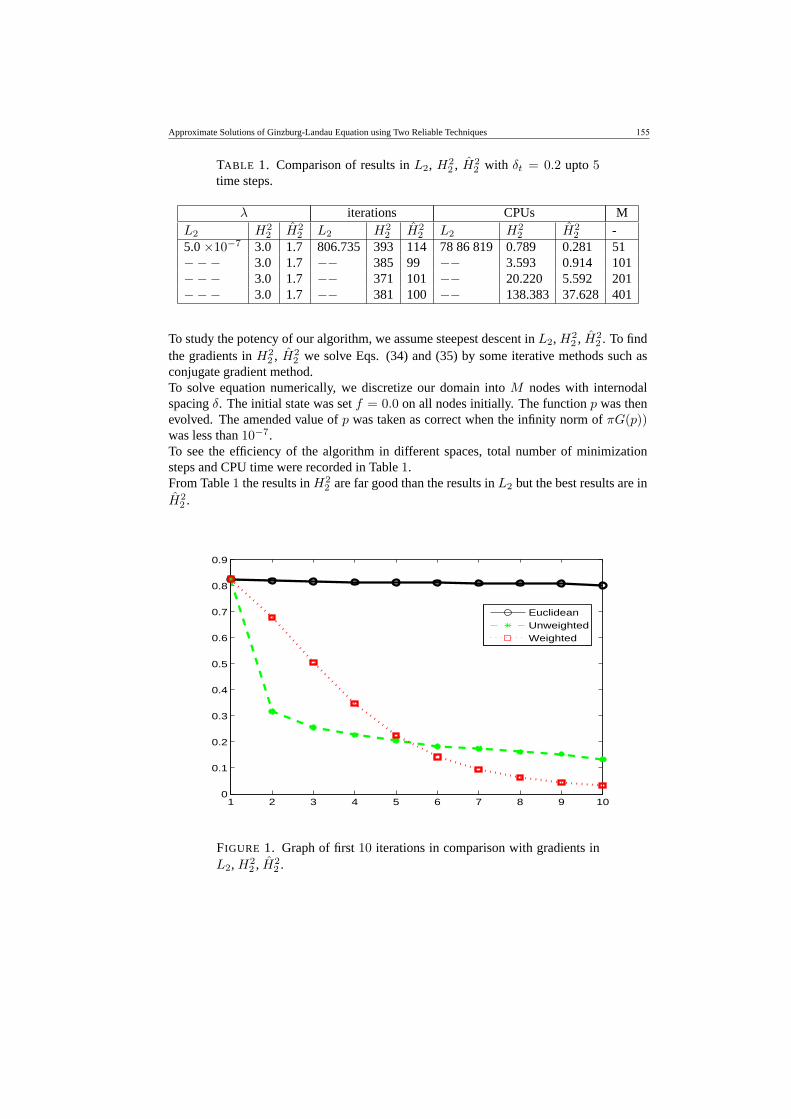
TABLE 1. Comparison of results inL2, H22 , H2

2 with δt = 0.2 upto 5time steps.

λ iterations CPUs ML2 H2

2 H22 L2 H2

2 H22 L2 H2

2 H22 -

5.0×10−7 3.0 1.7 806.735 393 114 7886819 0.789 0.281 51−−− 3.0 1.7 −− 385 99 −− 3.593 0.914 101−−− 3.0 1.7 −− 371 101 −− 20.220 5.592 201−−− 3.0 1.7 −− 381 100 −− 138.383 37.628 401

To study the potency of our algorithm, we assume steepest descent inL2, H22 , H2

2 . To findthe gradients inH2

2 , H22 we solve Eqs. (34) and (35) by some iterative methods such as

conjugate gradient method.To solve equation numerically, we discretize our domain intoM nodes with internodalspacingδ. The initial state was setf = 0.0 on all nodes initially. The functionp was thenevolved. The amended value ofp was taken as correct when the infinity norm ofπG(p))was less than10−7.To see the efficiency of the algorithm in different spaces, total number of minimizationsteps and CPU time were recorded in Table1.From Table1 the results inH2

2 are far good than the results inL2 but the best results are inH2

2 .

1 2 3 4 5 6 7 8 9 100

0.1

0.2

0.3

0.4

0.5

0.6

0.7

0.8

0.9

EuclideanUnweightedWeighted

FIGURE 1. Graph of first10 iterations in comparison with gradients inL2, H2

2 , H22 .

156 Nauman Raza

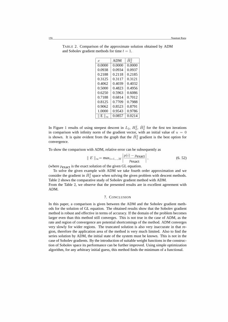
TABLE 2. Comparison of the approximate solution obtained by ADMand Sobolev gradient methods for timet = 1.

x ADM H22

0.0000 0.0000 0.00000.0938 0.0934 0.09370.2188 0.2118 0.21850.3125 0.3117 0.31210.4062 0.4039 0.40320.5000 0.4823 0.49560.6250 0.5963 0.60860.7188 0.6814 0.70120.8125 0.7709 0.79880.9062 0.8523 0.87911.0000 0.9543 0.9786‖ E ‖∞ 0.0857 0.0214

In Figure 1 resultsof using steepest descent inL2, H22 , H2

2 for the first ten iterationsin comparison with infinity norm of the gradient vector, with an initial value ofu = 0is shown. It is quite evident from the graph that theH2

2 gradient is the best option forconvergence.

To show the comparison with ADM, relative error can be subsequently as

‖ E ‖∞= maxi=1,..,M

∣∣∣∣p(i)− pexact

pexact

∣∣∣∣ , (6. 52)

(wherepexactis the exact solution of the given GL equation.To solve the given example with ADM we take fourth order approximation and we

consider the gradient inH22 space when solving the given problem with descent methods.

Table2 shows the comparative study of Sobolev gradient method with ADM.From the Table2, we observe that the presented results are in excellent agreement withADM.

7. CONCLUSION

In this paper, a comparison is given between the ADM and the Sobolev gradient meth-ods for the solution of GL equation. The obtained results show that the Sobolev gradientmethod is robust and effective in terms of accuracy. If the domain of the problem becomeslarger even than this method still converges. This is not true in the case of ADM, as therate and region of convergence are potential shortcomings of the method. ADM convergesvery slowly for wider regions. The truncated solution is also very inaccurate in that re-gion, therefore the application area of the method is very much limited. Also to find theseries solution by ADM, the initial state of the system must be known. This is not in thecase of Sobolev gradients. By the introduction of suitable weight functions in the construc-tion of Sobolev space its performance can be further improved. Using simple optimizationalgorithm, for any arbitrary initial guess, this method finds the minimum of a functional.

ApproximateSolutionsof Ginzburg-Landau Equation using Two Reliable Techniques 157

The choice of underlying space and gradient plays a vital role in the construction of efficientalgorithms. A number of different gradients can be defined from the same functional, whichhave different numerical properties. It is still an open problem as to how we can select asuitable space and define a gradient in it, such that it is best suited for the given problemexcept for linear problems [26].

REFERENCES

[1] R. A. Adams,Sobolev Spaces, Academic Press, 1975.[2] G. Adomian,Nonlinear Stochastic operator equations, Kluwer Acad. Publ. 1986.[3] G. Adomian,Solving frontiers problems of physics-The decomposition method, Kluwer Acad. Publ. 1994.[4] G. Adomian and R. E. Meyers,The Ginzburg-Landau Equation, Computer and Mathematics with Appl.29,

No. 3 (1995) 3-4.[5] A. Atangana and JF. Botha,Analytical solution of the groundwater flow equation obtained via homotopy

decomposition method, J. Earth Sci. Clim Chang3, No. 115 (2012) doi:10.4172/2157-7617.1000115.[6] A. Atangana and SB. Belhaouari,Solving partial differential equation with space-and time-fractional deriv-

atives via homotopy decomposition method, Math. Probl. Eng.9, (2013) doi:10. 1155/2013/318590.[7] M. Bayram et al.Approximate solutions some nonlinear evolutions equations by using the reduced differen-

tial transform method, Int. J. Appl. Math. Res.1, No. 3 (2012) 288302.[8] C. Beasley,Finite Element Solution to Nonlinear Partial Differential Equations, PhD Thesis, University of

North Texas, Denton, Tx. (1981).[9] N. Bildik et al Solution of different type of the partial differential equation by differential transform method

and Adomians decomposition method, Appl. Math. Comp.172, No. 1 (2006) 551567.[10] N. Bildik and S. Deniz,Implementation of Taylor collocation and Adomian decomposition method for sys-

tems of ordinary differential equations, AIP Publ.1648, (2015) 370002.[11] N. Bildik and A. Konuralp,The use of variational iteration method, differential transform method and

Adomian decomposition method for solving different types of nonlinear partial differential equations, Int. J.Nonlinear Sci. Numer. Simul.7, No. 1 (2006) 6570.

[12] N. Bildik, M. Tosun and S. Deniz,Euler matrix method for solving complex differential equations withvariable coefficients in rectangular domains, Int. J. Applied Phys. Math.7, No. 1 (2017) 69.

[13] N. Bildik and S. Deniz,A Practical Method for Analytical Evaluation of Approximate Solutions of Fisher’sEquations, ITM Web of Conferences,13, EDP Sciences, 2017.

[14] N. Bildik and S. Deniz,Comparative study between optimal homotopy asymptotic method and perturbation-iteration technique for different types of nonlinear equations,Iran. J. Sci. Technol. Trans. Sci.42, No. 2(2018) 647-654.

[15] B. Brown, M. Jais and I. Knowles,A variational approach to an elastic inverse problem, Inverse Problems21, (2005) 1953-1973.

[16] H. Bulut, M. Ergut and D. Evans,The numerical solution of multidimensional partial differential equationsby the decomposition method, Int. J. Comp. Math.80, No. 9 (2003) 1189-1198.

[17] J. T. Edwards, J. Roberts and N. Ford,A comparison of Adomian’s decomposition method and Runge Kuttamethods for approximate solution of some predator prey model equations, University of Manchester, Nu-merical analysis Report No. 309, 1997

[18] J-H. He,Variational iteration methoda kind of non-linear analytical technique: some examples, Int. J. Non.Linear Mech.34, No. 4 (1999) 699708.

[19] J-H. He,Homotopy perturbation method for bifurcation of nonlinear problems, Int. J. Nonlinear Sci. NumerSimul.6, No. 2 (2005) 207208.

[20] J. Karatson and I. Farago,Preconditioning operators and Sobolev gradients for nonlinear elliptic problems,Comput. Math. Appl.50, (2005) 1077-1092.

[21] J. Karatson,Constructive Sobolev gradient preconditioning for semilinear elliptic systems, Electron J. Dif-ferential Equations75, (2004) 1-26.

[22] J. Karatson and L. Loczi,Sobolev gradient preconditioning for the electrostatic potential equation, Comput.Math. Appl.50, (2005) 1093-1104.

158 Nauman Raza

[23] H. Khalil, R. A. Khan, M. H. Al-Smadi and A. A. Freihat, Approximation of Solution of Time Fractional Order Three-Dimensional Heat Conduction Problems with Jacobi Polynomials, Punjab Univ. j. math. 47, No. 1 (2015) 35-56.

[24] I. Knowles and A. Yan, On the recovery of transport parameters in groundwater modelling, J. Comp. Appl.Math. 171, (2004) 277-290.

[25] W. T. Mahavier, A numerical method utilizing weighted Sobolev descent to solve singluar differential equa-tions, Nonlinear World 4, No. 4 (1997).

[26] W. T. Mahavier and J. Montgomery, Single Iteration Sobolev descent for linear initial value Problems,Missouri J. Math. Sci. 25, No. 1 (2013) 15-26.

[27] J. W. Neuberger, Sobolev Gradients and Differential Equations, Springer Lecture Notes in Mathematics 1670 (Springer-Verlag, 1997).

[28] R. Nittka and M. Sauter, Sobolev gradients for differential algebraic equations, J. Differ. Equ. 42, (2008)1-31.

[29] T. Ozis and D. Agirseven, He’s homotopy perturbation method for solving heat-like and wave-like equations with variable coefficients, Phys Lett A 372, No. 38 (2008) 5944-5950.

[30] N. Raza, Application of Sobolev Gradient Method to Solve Klein Gordon Equation, Punjab Univ. j. math. 48, No. 2 (2016) 135-145.

[31] N. Raza, S. Sial and S. Siddiqi, Sobolev gradient approach for the time evolution related to Energy mini-mization of Ginzberg-Landau functionals, J. Comp. Phys. 228, (2009) 2566-2571.

[32] N. Raza, S. Sial and S.S. Siddiqi, Approximating time evolution related to Ginzberg-Landau functionals viaSobolev gradient methods in a finite-element setting, J. Comp. Phys. 229, (2010) 1621-1625.

[33] A. U. Rehman, S. U. Rehman and J. Ahmad, Numerical Approximation of Stiff Problems Using Efficient Nested Implicit RungeKutta Methods, Punjab Univ. j. math. 51, No. 2 (2019) 1-19.

[34] S. Sial, J. W. Neuberger, T. Lookman and A. Saxena, Energy minimization using Sobolev gradients: Appli-cation to phase separation and ordering, J. Comp. Phys. 189, (2003) 88-97.

[35] S. Sial, J. Neuberger, T. Lookman and A. Saxena, Energy minimization using Sobolev gradients finite el-ement setting, Proc. World Conference on 21st Century Mathematics, Lahore, Pakistan, March 2005 eds.Chaudhary and Bhatti.

[36] S. Sial, Sobolev gradient algorithm for minimum energy states of s-wave superconductors: finite element setting, Supercond. Sci. Technol. 18, (2005) 675-677.

[37] M. Suleman and S. Riaz, Unconditionally Stable Numerical Scheme to Study the Dynamics of Hepatitis BDisease, Punjab Univ. j. math. 49, No. 3 (2017) 99-118.

[38] A. M. Wazwaz, A comparison between Adomian decomposition method and Taylor series method in theseries solutions, Applied Mathematics and Computation 97, (1997) 37-44.