Approximate simulation techniques and distribution of an

HAL Id: hal-01247062https://hal.archives-ouvertes.fr/hal-01247062

Submitted on 27 Dec 2015

HAL is a multi-disciplinary open accessarchive for the deposit and dissemination of sci-entific research documents, whether they are pub-lished or not. The documents may come fromteaching and research institutions in France orabroad, or from public or private research centers.

L’archive ouverte pluridisciplinaire HAL, estdestinée au dépôt et à la diffusion de documentsscientifiques de niveau recherche, publiés ou non,émanant des établissements d’enseignement et derecherche français ou étrangers, des laboratoirespublics ou privés.

Distributed under a Creative Commons Attribution| 4.0 International License

Approximate simulation techniques and distribution ofan extended Gamma process

Zeina Al Masry, Sophie Mercier, Ghislain Verdier

To cite this version:Zeina Al Masry, Sophie Mercier, Ghislain Verdier. Approximate simulation techniques and distributionof an extended Gamma process. Methodology and Computing in Applied Probability, Springer Verlag,2017, 19 (1), pp.213-235. �10.1007/s11009-015-9474-3�. �hal-01247062�

https://hal.archives-ouvertes.fr/hal-01247062

http://creativecommons.org/licenses/by/4.0/

http://creativecommons.org/licenses/by/4.0/

https://hal.archives-ouvertes.fr

Noname manuscript No.(will be inserted by the editor)

Approximate simulation techniques and distribution of anextended Gamma process

Zeina AL MASRY · Sophie MERCIER · GhislainVERDIER

Received: date / Accepted: date

Abstract In reliability theory, many papers use a standard Gamma process to model theevolution of the cumulative deterioration of a system over time. When the variance-to-meanratio of the system deterioration level varies over time, the standard Gamma process is notconvenient any more because it provides a constant ratio. A way to overcome this restrictionis to consider the extended version of a Gamma process proposed by Cinlar (1980). How-ever, based on its technicality, the use of such a process for applicative purpose requires thepreliminary development of technical tools for simulating its paths and for the numericalassessment of its distribution. This paper is devoted to these two points.

Keywords Reliability · Degradation · Process with independent increments · Seriesrepresentation · Inverse Laplace transform · Post-Widder formula · Weighted Gammaprocess

1 Introduction

Safety and dependability is a crucial issue in many industries, which has lead to the develop-ment of a huge literature devoted to the so-called reliability theory. In the oldest literature,the lifetimes of industrial systems or components were usually directly modeled throughrandom variables, see e.g. Barlow and Proschan (1965) for a pioneer work on the subject.Based on the development of on-line monitoring which allows the effective measurement ofa system deterioration, numerous papers nowadays model the degradation in itself, whichoften is considered to be accumulating over time. This is done through the use of a nondecreasing stochastic process (Xt)t≥0 (say), where the system lifetime τ typically corre-sponds to the hitting time of a given failure threshold L:

τ = inf(t > 0 : Xt > L).

Laboratoire de Mathematiques et de leurs Applications - Pau (UMR CNRS 5142)Universite de Pau et des Pays de l’Adour, Batiment IPRA, Avenue de l’Universite,F-64013 PAU cedex, FRANCETel.: +33 (0)5 59 40 75 37Fax: +33 (0)5 59 40 75 55E-mail: [email protected], [email protected],[email protected]

2 Zeina AL MASRY et al.

A major quantity of interest for such a system is its reliability function R(t), which corre-sponds to the probability that, without any repair, the system is still in order at time t:

R(t) = P(τ > t) = P(Xt ≤ L) = FXt(L) =

∫ L

0

fXt(s) ds,

where FXtand fXt

stand for the cumulative distribution function (cdf) and probability den-sity function (pdf) of Xt, respectively. Another important indicator for prediction purposeis the system Mean Time Before Failure (MTBF), with

MTBF = E(τ) =

∫ ∞0

P(τ > t) dt =

∫ ∞0

FXt(L) dt.

Most of other quantities of interest (Mean Residual Lifetime, cost/profit functions, . . . )may also be expressed with respect to the pdf or cdf of Xt, e.g. see Rausand and Høyland(2004). Before being able to use a stochastic process (Xt)t≥0 for deterioration modelingpurpose and make prediction over the system future behavior, there hence is a crucial needto develop tools for computing its pointwise pdf and cdf at time t and/or for simulating tra-jectories of (Xt)t≥0, which provides another way to compute the aimed quantities throughMonte-Carlo simulations.

Since seminal papers (Abdel-Hameed 1975) and (Cinlar et al 1977), the most widelyused process to model the phenomena of cumulative degradation is the (standard) Gammaprocess, see van Noortwijk (2009) for a comprehensive presentation and overview of appli-cations of the Gamma process to reliability theory, including more than 100 references andboth scientific and empirical justification of its use. However, a notable restriction of a stan-dard Gamma process is that its variance-to-mean ratio is constant over time, which may berestrictive within an applicative context, see Guida et al (2012) for a real data set consistingof ”sliding wear data of four metal alloy specimens” and where there is ”empirical evidencethat the variance-to-mean ratio is not a constant but varies with [time]”. To overcome thisdrawback, we propose to use an Extended Gamma Process (EGP), which was introducedmostly simultaneously by Cinlar (1980) and Dykstra and Laud (1981). Note that EGPs arealso called weighted Gamma processes in the literature (Ishwaran and James 2004). AnEGP is a non decreasing process with independent increments, which can be constructed asa stochastic integral with respect to a standard Gamma process. If the EGP has been usedfor Bayesian modeling of the hazard function (Dykstra and Laud 1981; Ishwaran and James2004; Laud et al 1996), up to our knowledge, it has not been much studied for cumulativedegradation modeling, except in Guida et al (2012) in a simplified setting.

A standard Gamma process is characterized by a shape function and a constant scaleparameter. For an EGP, the scale parameter may vary over time. This allows for more flex-ibility than its standard version, for modeling purpose. However, there is a cost and the useof an EGP presents some technical difficulties. Firstly, except for specific cases, the exactsimulation of such a process is generally impossible. Secondly, there is no explicit formulafor the probability distribution of an EGP (which is not Gamma). These technical difficultieshave lead Guida et al (2012) to use a discrete version of an EGP. We here propose to dealwith the original continuous time version.

The aim of the present paper is to develop technical tools necessary to the practical useof an EGP for cumulative degradation modeling (or for any other purpose). More precisely,we focus on the simulation of approximate sample paths and on the numerical assessment ofboth its pdf and cdf. Our contribution is threefold. Firstly, the series representations providedby Rosinski (2001) for standard Gamma processes are extended to EGPs. Such representa-tions are used to generate approximate sample paths. The quality of the approximation is

Approximate simulation techniques and distribution of an extended Gamma process 3

studied and compared to the method proposed by Ishwaran and James (2004), which isbased on an alternate approximate representation of an EGP. Secondly, following the re-sults of Veillette and Taqqu (2011) for Laplace transform inversion through Post-Widderformulas, explicit asymptotic expressions are provided for both pdf and cdf of an EGP.Thirdly, a discretization method is proposed, based on the approximation of a general EGPby a specific EGP with a piecewise constant scale function, which is easy to deal with. Thediscretization method allows both to simulate approximate sample paths of a general EGPand to compute approximations of its pdf and cdf. Convergence results are obtained for theapproximate discretized EGP towards the initial general EGP and the quality of the approx-imation is studied. The method allows to compute the cdf of a general EGP at a known andadjustable precision. Up to our knowledge, a similar result was not available in the previousliterature.

The paper is organized as follows. Section 2 gives an overview of the EGP. In Section3, the approximate representation of Ishwaran and James (2004) is presented as well as fourseries representations of an EGP. Section 4 is devoted to the approximation of the pdf andcdf through Laplace transform inversion. Section 5 introduces and studies the discretizationmethod. The different methods are illustrated through numerical experiments in Section 6.Conclusions are formulated in Section 7.

2 Definition of an EGP and first properties

Let a : R+ → R+ be a measurable, increasing and right-continuous function with a(0) = 0and let b0 > 0. Recall that a standard (non homogeneous) Gamma process Γ0(a(t), b0)with a(.) as shape function and b0 as (constant) scale parameter is a stochastic process withindependent, non-negative and Gamma distributed increments. Its pdf at a specified timepoint t is given by

ft(x) =ba(t)0

Γ (a(t))xa(t)−1 exp(−b0x),∀x ≥ 0,

e.g. see Abdel-Hameed (1975).

Now, let b : R∗+ → R∗+ be a measurable positive function such that, for all t > 0:∫(0,t]

da(s)

b(s)<∞. (1)

Following (Cinlar 1980; Dykstra and Laud 1981), the process X = (Xt)t≥0 is said tobe an EGP with shape function a(.) and scale function b(.) (written X ∼ Γ (a(t), b(t)) inthe sequel) if it can be represented as a stochastic integral with respect to a standard Gammaprocess (Yt)t≥0 ∼ Γ0(a(t), 1):

Xt =

∫(0,t]

dYsb(s)

, ∀t > 0 (2)

and X0 = 0.If b(.) is constant and equal to b0, the EGP simply reduces to a standard Gamma process

Γ0(a(t), b0). An EGP can be proved to have independent increments and its distribution to


be infinitely divisible (Cinlar 1980). Also, an explicit formula is available for the Laplacetransform of an increment, with

LXt+h−Xt(λ) := E

(e−λ(Xt+h−Xt)

)= exp

(−∫(t,t+h]

log

(1 +

λ

b(s)

)da(s)

),

(3)for all t, λ ≥ 0 and h > 0.

Conversely, a stochastic process with independent increments and Laplace transform ofan increment provided by (3) can be proved to be an EGP ∼ Γ (a(t), b(t)).

Finally, the mean and variance of an EGP are given by

E(Xt) =

∫(0,t]

da(s)

b(s)and V(Xt) =

∫(0,t]

da(s)

b(s)2. (4)

Remark 1 Let X ∼ Γ (a(t), b(t)). So far, the shape function a was supposed to be right-continuous. Then, following Cinlar (1980), the function a can be written as a = ac + ad,where ac is the continuous part of a and ad its jump part. The EGP X is then the sum oftwo independent EGPs Xc ∼ Γ (ac(t), b(t)) and Xd ∼ Γ (ad(t), b(t)). This second EGPsimply reduces, for each t ≥ 0, to a sum of independent Gamma variables, for which thedistribution is known in full form (see Section 5). This second EGP is hence easy to dealwith and can be omitted without loss of generality. Thus, the shape function a is assumed tobe continuous in the sequel.

For a better understanding of the possible evolution of an EGP over time, we now lookat its asymptotic behavior and we set

X∞ = limt→∞

Xt (≤ ∞),

which exists, due to the non decreasingness property of an EGP.

Proposition 1 Let X = (Xt)t≥0 be an EGP with X ∼ Γ (a(t), b(t)). We then have:∫(0,∞)

log

(1 +

1

b(s)

)da(s) ≤ E(X∞) =

∫(0,∞)

da(s)

b(s)≤ ∞ (5)

and the following results:

1. If E(X∞) <∞, then X∞ is almost surely finite.2. If ∫

(0,∞)

log

(1 +

1

b(s)

)da(s) =∞, (6)

then X∞ is almost surely infinite.

Proof Inequation (5) and the first point are clear. For the second one, let us note that

E(e−X∞) = LX∞(1) = exp

(−∫(0,∞)

log

(1 +

1

b(s)

)da(s)

).

Under assumption (6), we consequently have E(e−X∞) = 0. This implies that e−X∞ = 0almost surely and the result.


Remark 2 In the case where∫(0,∞)

log

(1 +

1

b(s)

)da(s) <∞ =

∫(0,∞)

da(s)

b(s), (7)

the dichotomy P (X∞ =∞) ∈ {0, 1} is not valid any more and both P (X∞ =∞) > 0and P (X∞ <∞) > 0 are possible, as is illustrated in the following example (third case).

Example 1 The different types of behavior are illustrated in Figure 1, 2 and 3 (left) where afew sample paths are plotted for three different EGPs (using the discretized rate method fromSection 5): X(1) ∼ Γ (t, (t + 1)2), X(2) ∼ Γ

(t, 1

(t+1)2

)and

X(3) ∼ Γ(

12

(1− 1

(t+1)2

), 1exp(1+t)−1

). The process X(1) (resp. X(2)) corresponds

to the first (resp. second) case of Proposition 1 whereas X(3) corresponds to case (7). Asexpected, all trajectories of Figure 1 are stabilizing whereas all trajectories of Figure 2 areexploding. In Figure 3, some trajectories are exploding and others are stabilizing. For a betterinsight into their behavior, the variance-to-mean ratios of the X(i)’s are also plotted in thesame figures (right). These figures illustrate the flexibility of EGPs for modeling purpose.

In all the following,X = (Xt)t≥0 stands for an EGP∼ Γ (a(t), b(t)) and Y = (Yt)t≥0

stands for a standard Gamma process Γ0(a(t), 1), without any further notification. We recallthat the shape function a(t) is assumed to be continuous.

3 Simulation techniques of an EGP

The goal of this section is to present methods for generating approximate sample paths ofan EGP on a given compact set [0, T ]. The section is divided into two parts. The first partquickly recalls the method proposed by Ishwaran and James (2004). In the second part,the series representations of a standard Gamma process provided in Rosinski (2001) areextended to the case of an EGP. Algorithms based on these series representations are furtherprovided in Section 6 for approximate sample paths generation.

3.1 Ishwaran and James’s method

The method proposed by Ishwaran and James (2004) roughly boils down to some discretiza-tion of the stochastic integral (2) for t ∈ [0, T ], where T > 0. More specifically, for eacht ∈ [0;T ] and each K∗ ∈ N, they consider:

G(K∗)t =

K∗∑k=1

1[0,t](Vk)1

b(Vk)W

(K∗)k , (8)

where (Vk)k=1,...K∗ are i.i.d random variables (r.v.s) with distribution da(v)a(T ) 1[0,T ](v) and

(W(K∗)k )k=1,...K∗ are i.i.d r.v.s with Gamma distribution Γ0(a(T )

K∗ , 1), independent fromthe Vk’s.Ishwaran and James (2004) proved that

(G

(K∗)t

)t≥0−→ (Xt)t≥0 weakly whenK∗ →∞

in the Skorokhod space D (0,∞) of right-continuous functions with left-side limits. (To be


0 0.2 0.4 0.6 0.8 10.5

0.6

0.7

0.8

0.9

1

V(X

(1)

t)/E(X

(1)

t)

t0 2 4 6 8 10

0

0.5

1

1.5

2

X(1

)t

tFig. 1 Sample paths (left) and ratio V(X(1)

t )

E(X(1)t )

(right) as a function of time

0 2 4 6 8 100

200

400

600

800

X(2

)t

t0 0.2 0.4 0.6 0.8 1

1

1.5

2

2.5

3V(X

(2)

t)/E(X

(2)

t)


t )

E(X(2)t )


0 2 4 6 8 100

20

40

60

80

100

X(3

)t

t0 0.2 0.4 0.6 0.8 1

1.5

2

2.5

3

3.5

V(X

(3)

t)/E(X

(3)

t)


t )

E(X(3)t )


more specific, they show the weak convergence of the random measure with correspondingcumulative process defined by (8) towards a weighted gamma measure with shape measurea(dt) and scale function b(t). The weak convergence of the cumulative process (8) towardsan EGP is then a consequence of (Daley and Vere-Jones 2007, Lemma 11.1.XI)).


One can easily check that

E[G

(K∗)t

]= E[Xt],

V[G

(K∗)t

]= V[Xt] +

1

K∗

(a(T )V[Xt]− (E[Xt])

2)

so that the approximation of Xt by G(K∗)t is unbiased. Also, the rate of convergence of the

variance is O(

1K∗

).

3.2 Series representations

The following results extend those from (Rosinski 2001, Section 6) devoted to standardGamma processes, see Rosinski (2001) for more references and historical remarks.

Proposition 2 Let T > 0 and let (Un)n≥1 be the points of a homogeneous Poisson processM with parameter a(T ). Let also (Vn)n≥1 be a sequence of i.i.d. r.v.s with distributionH(dv) = da(v)

a(T ) 1[0,T ](v), independent of M and let (Wn)n≥1 be a sequence of i.i.d r.v.swith distribution PW (dw), independent of M and of the Vn’s. Then we have the four fol-

lowing series representations of an EGP, where D= means ”is identically distributed as”:

(1) Bondesson’s series representation (Bond):

XtD=∑n≥1

1

b(Vn)exp(−Un) Wn1[0,t](Vn), for 0 ≤ t ≤ T, (9)

where {Wn}n≥1 is a sequence of i.i.d exponential r.v.s with mean 1,(2) Rejection’s series representation (Rej):

XtD=∑n≥1

1

b(Vn)

1

exp(Un)− 11E (Un,Wn)1[0,t](Vn), for 0 ≤ t ≤ T, (10)

whereE ={

(u,w) ∈ R+ × [0, 1] | exp(u)exp(u)−1 exp(−(exp(u)− 1)−1) ≥ w

}and where

{Wn}n≥1 is a sequence of i.i.d uniform r.v.s on [0, 1],(3) Thinning’s series representation (Thin):

XtD=∑n≥1

1

b(Vn)Wn1(WnUn≤1)1[0,t](Vn), for 0 ≤ t ≤ T, (11)

where {Wn}n≥1 is a sequence of i.i.d exponential r.v.s with mean 1,(4) Inversion of Levy measure’s series representation (ILM):

XtD=∑n≥1

1

b(Vn)E−1

1 (Un)1[0,t](Vn), for 0 ≤ t ≤ T, (12)

with E1(x) =∫∞xu−1 exp(−u)du, the exponential integral function.


Proof The four series representations can be written in the same manner:

Xt =∑n≥1

ft(Un, Vn,Wn) =∑n≥1

1

b(Vn)H(Un,Wn)1[0,t](Vn), (13)

with ft(u, v, w) = 1b(v)H(u,w)1[0,t](v) and an appropriate choice for H : R2

+ → R+.As already mentioned in Section 2, (Xt)0≤t≤T is an EGP if its increments are independentand the Laplace transform of an increment can be written as in (3). Let us first note that(Un, Vn,Wn)n≥1 can be seen as the points of a Poisson random measure N on R3

+ withintensity

µ(du, dv, dw) = du× da(v)1[0,T ](v)× PW (dw)

(see for example (Cınlar 2011, Corollary 3.5, p. 265)).Considering t1 < · · · < tn, we then have Xti+1 − Xti = N(fti+1 − fti) for all

1 ≤ i ≤ n − 1, where fti+1 − fti takes range in R+ × (ti, ti+1] × R+. As the ranges ofthe fti+1 − fti are non overlapping, the increments Xti+1 −Xti are independent.

Now, based on the Laplace functional theorem for a Poisson random measure (Cınlar2011, Theorem 2.9, p. 252) for the third line, we have for all t ∈ [0, T ] and all h, λ > 0:

LXt+h−Xt(λ)

= E[exp(−λ(Xt+h −Xt))]= E[exp(−N(λ(ft+h − ft)))]

= exp

(−∫R3

(1− e−(λ(ft+h−ft))

))dµ

= exp

(−∫(t,t+h]

Q(λ, v)da(v)

)(14)

where

Q(λ, v) =

∫R2

(1− exp

(−λ 1

b(v)H(u,w)

))du× PW (dw).

From (3) and (14), it then suffices to check that Q(λ, v) = log(

1 + λb(v)

)for each of the

four series representations.

1) Bondesson:In this case, H(u,w) = exp(−u)w and PW (dw) = exp(−w)dw. Then

Q(λ, v) =

∫ ∞0

(∫ ∞0

(1− exp

(− λ

b(v)exp(−u)w

))exp(−w)dw

)du

=

∫ ∞0

(1− b(v)

b(v) + λ exp(−u)

)du

=

∫ ∞0

(λ exp(−u)

b(v) + λ exp(−u)

)du

= log

(1 +

λ

b(v)

).


2) Rejection:Here,H(u,w) = 1

exp(u)−11(exp(u)

exp(u)−1exp(− 1

exp(u)−1)≥w)

and PW (dw) = dw. Accord-

ingly,

Q(λ, v) =

∫ ∞0

(∫ exp(u)

exp(u)−1exp(− 1

exp(u)−1)

0

(1− exp

(− λ

b(v)

1

exp(u)− 1

))dw

)du

=

∫ ∞0

(1− exp

(− λ

b(v)

1

exp(u)− 1

))exp(u)

exp(u)− 1exp

(− 1

exp(u)− 1

)du

=

∫ ∞0

(1− exp

(− λ

b(v)z

))exp(−z)

zdz (15)

setting z = 1exp(u)−1 in the last line.

(15) is a Frullani’s integral, which can classically be computed by differentiating withrespect of λ: Setting o(λ, v, z) =

(1− exp

(− λb(v)z

))exp(−z)

z , we get by dominatedconvergence that

∂Q(λ, v)

∂λ=

∫ ∞0

∂o(λ, v, z)

∂λdz =

1

b(v) + λ,

which provides the result.

3) Thinning:H(u,w) = w1(uw≤1) and PW (dw) = exp(−w)dw.

Q(λ, v) =

∫ ∞0

(∫ 1w

0

(1− exp

(− λ

b(v)w

))exp(−w)du

)dw

=

∫ ∞0

(1− exp

(− λ

b(v)w

))exp(−w)

wdw.

We recognize (15), which allows to conclude.

4) Inversion of Levy measure:H(u,w) = E−1

1 (u) is independent on w. Then

Q(λ, v) =

∫ ∞0

(1− exp

(− λ

b(v)E−1

1 (u)

))du

=

∫ ∞0

(1− exp

(− λ

b(v)z

))exp(−z)

zdz

setting z = E−11 (u). We recognize (15) again, which allows to conclude.

Approximate simulation of (Xt)0≤t≤T is done by truncating the infinite series. As isclassically done in the Levy case, we retain only the points of the Poisson process M whichbelong to a compact set [0, B], where B > 0:

X(B)t =

∑n≥1

1

b(Vn)H(Un,Wn)1[0,t](Vn)1[0,B](Un)


for all t ∈ [0, T ], where we use the notations of (13). This allows to better control thetruncation error than simply retaining a fixed number of terms in the series, see e.g. Imaiand Kawai (2013) for further details in the Levy case. We also set

X(B)t = Xt −X(B)

t =∑n≥1

1

b(Vn)H(Un,Wn)1[0,t](Vn)1(B,∞)(Un) (16)

for all t ∈ [0, T ], to be the remainder of the truncated series. By construction, both(X

(B)t

)t∈[0,T ]

and(X

(B)t

)t∈[0,T ]

have independent increments. The moments of X(B)t are given in the

following proposition.

Proposition 3 Recall that X(B)t is the remainder of the truncated series (16). We have

(1) Bondesson’s series representation:

X(B)t ∼ Γ

(a(t),

b(t)

exp(−B)

);

E[X(B)t ] = exp(−B)E[Xt];

V[X(B)t ] = exp(−2B)V[Xt],

(2) Rejection’s series representation:

E[X(B)t ] = E[Xt]

[1− exp

(− 1

exp(B)− 1

)];

V[X(B)t ] = V [Xt]

[1−

(1 +

1

exp(B)− 1

)exp

(− 1

exp(B)− 1

)],

(3) Thinning’s series representation:

E[X(B)t ] = E[Xt]

[1−B +B exp

(− 1

B

)];

V[X(B)t ] = V[Xt]

[1 + exp

(− 1

B

)+ 2B exp

(− 1

B

)− 2B

],

(4) Inversion of Levy measure’s series representation:

E[X(B)t ] = E[Xt](1− E1(B));

V[X(B)t ] = V[Xt](1− exp(−E1(B))− E1(B) exp(−E1(B))).

Proof Starting from (16), the Laplace transform of X(B)t is computed using the Laplace

functional theorem for Poisson random measures. In the Bondesson case, we recognize theLaplace transform of an EGP ∼ Γ

(a(t), b(t)

exp(−B)

). For the three other representations,

the mean and variance are obtained through the first and second order derivatives of theLaplace transform at λ = 0.

Proposition 3 allows to determine the minimal value ofB which ensures a given relativeprecision on both mean and variance of Xt for all t ∈ [0, T ] (analytically for Bondesson’sseries representation and numerically for the three other procedures). Asymptotic equiva-lents of the series remainders are provided in Table 1 when B tends to infinity, which areobtained through Taylor expansions.


Method E(X

(B)t

)/E(Xt) V

(X

(B)t

)/V(Xt)

Bondesson exp(−B) exp(−2B)

Rejection exp(−B)exp(−2B)

2

Thinning 12B

16B2

Inversion of Levy measure E1(B)E1(B)2

2

Table 1 Asymptotic equivalents of E(X

(B)t

)/E(Xt) and V

(X

(B)t

)/V(Xt) when B →∞

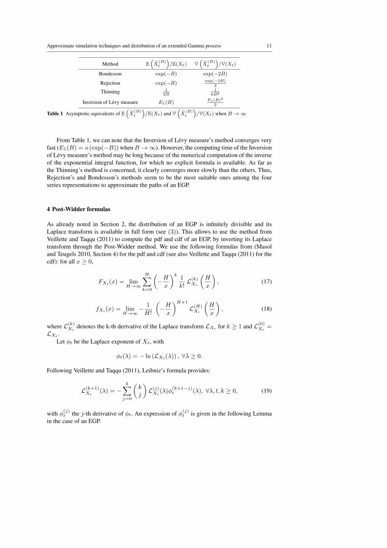
From Table 1, we can note that the Inversion of Levy measure’s method converges veryfast (E1(B) = o (exp(−B)) whenB →∞). However, the computing time of the Inversionof Levy measure’s method may be long because of the numerical computation of the inverseof the exponential integral function, for which no explicit formula is available. As far asthe Thinning’s method is concerned, it clearly converges more slowly than the others. Thus,Rejection’s and Bondesson’s methods seem to be the most suitable ones among the fourseries representations to approximate the paths of an EGP.

4 Post-Widder formulas

As already noted in Section 2, the distribution of an EGP is infinitely divisible and itsLaplace transform is available in full form (see (3)). This allows to use the method fromVeillette and Taqqu (2011) to compute the pdf and cdf of an EGP, by inverting its Laplacetransform through the Post-Widder method. We use the following formulas from (Masoland Teugels 2010, Section 4) for the pdf and cdf (see also Veillette and Taqqu (2011) for thecdf): for all x ≥ 0,

FXt(x) = lim

H→∞

H∑k=0

(−Hx

)k1

k!L(k)Xt

(H

x

), (17)

fXt(x) = lim

H→∞− 1

H!

(−Hx

)H+1

L(H)Xt

(H

x

), (18)

where L(k)Xt

denotes the k-th derivative of the Laplace transform LXtfor k ≥ 1 and L(0)

Xt=

LXt.Let φt be the Laplace exponent of Xt, with

φt(λ) = − ln (LXt(λ)) , ∀λ ≥ 0.

Following Veillette and Taqqu (2011), Leibniz’s formula provides:

L(k+1)Xt

(λ) = −k∑j=0

(kj

)L(j)Xt

(λ)φ(k+1−j)t (λ), ∀λ, t, k ≥ 0, (19)

with φ(j)t the j-th derivative of φt. An expression of φ(j)

t is given in the following Lemmain the case of an EGP.


Lemma 1 Let λ ≥ 0, j ≥ 1 and let X ∼ Γ (a(t), b(t)).Then

φ(j)t (λ) = (−1)j−1(j − 1)! m

(j)t (λ)

where

m(j)t (λ) =

∫ t

0

da(s)

(b(s) + λ)j.

Proof Based on (3) and (15) and setting u = z/b(s) in the third line we have:

φt(λ) =

∫(0,t]

log

(1 +

λ

b(s)

)da(s)

=

∫(0,t]

(∫ ∞0

(1− exp

(− λ

b(s)z

))exp(−z)

zdz

)da(s)

=

∫ ∞0

(1− e−λu

)µt(du)

where

µt(du) =1

u

(∫(0,t]

e−b(s)uda(s)

)du

is a measure on R+ such that∫R+

(1 ∧ x)µt(dx) < ∞. From Veillette and Taqqu (2011),

φ(j)t (λ) is directly calculated by

φ(j)t (λ) = (−1)j+1

∫ ∞0

xje−λxµt(dx) (20)

for all j ≥ 1. This provides:

φ(j)t (λ) = (−1)j+1

∫ t

0

(∫ ∞0

xj−1e−(b(s)+λ)xdx

)da(s)

= (−1)j+1

∫ t

0

Γ (j)

(b(s) + λ)jda(s),

renormalizing the pdf of Γ0(j, b(s) + λ) to get the last line.

Based on (19) and Lemma 1, L(k)Xt

(λ) can be recursively computed through

L(k+1)Xt

(λ) = −k!k∑j=0

L(j)Xt

(λ)(−1)k−j

j!m

(k+1−j)t (λ) .

This allows to compute an approximation of the pdf and cdf of an EGP through (17− 18),taking H large enough.

5 Discretized rate function method

In case of a piecewise constant scale function b(.), the process (Xt)t≥0 can easily be con-structed from standard Gamma processes. The simulation of its paths is hence immediate(see e.g. van Noortwijk (2009)). Also, the random variable Xt simply is the sum of stan-dard Gamma variables, and different tools are available in the literature to compute both itspdf and cdf (see Nadarajah (2008) for a review). Based on this, the aim of this section is topropose an approximation of an EGP with a general scale function by another EGP with apiecewise constant scale function.


5.1 Construction of the approximate process X(ε)

Let T > 0. The following assumption is considered:

b(.) is continuous on (0, T ] and ∃m > 0 such that ∀t ∈ (0, T ], b(t) ≥ m. (21)

Let ε > 0. The following piecewise constant approximation of 1b(.) on (0, T ], denoted by

1b(ε)(.)

, is considered:

∀t ∈ (0, T ],1

b(ε)(t)=

n(ε)∑i=0

1

bi1[li,li+1)(t) (22)

where n(ε) is such that ln(ε) ≤ T < ln(ε)+1, l0 = 0, and the li’s, for i = 1, . . . , n(ε) + 1,are recursively defined by:

li+1 = sup

{l ∈ (li, T ] : ∀l′ ∈ [li, l],

∣∣∣∣ 1

b(li)− 1

b(l′)

∣∣∣∣ < ε

}. (23)

Note that assumption (21) insures that n(ε) is finite.The constants bi, i = 0, . . . , n(ε) are next defined by:

∀i = 0, . . . , n(ε)− 1,1

bi=

1

li+1 − li

∫ li+1

li

1

b(s)ds, (24)

and

1

bn(ε)=

1

T − ln(ε)

∫ T

ln(ε)

1

b(s)ds. (25)

Now that b(ε)(.) is constructed, we set

X(ε)t =

∫(0,t]

dYsb(ε)(s)

, ∀t ∈ [0, T ], (26)

where (Yt)t≥0 is the same standard Gamma process Γ0(a(t), 1) as in Equation (2) defining

X . Then(X

(ε)t

)t∈[0,T ]

is the restriction to [0, T ] of an EGP ∼ Γ(a(t), b(ε)(t)

)with the

same shape function a(.) as X and with b(ε)(.) as scale function.

Remark 3 Based of the definition (2) of an EGP, we prefer to construct an approximationof 1

b(.) instead of b (.). Also, by construction, for all t in (0, T ],

∣∣∣∣ 1

b(t)− 1

b(ε)(t)

∣∣∣∣ ≤ ε. (27)


5.2 Quality of the approximation of X by X(ε)

We first look at the moments of the residual part in the approximation of Xt by X(ε)t , for

t ∈ [0, T ].

Proposition 4 Let

X(ε)t = Xt −X(ε)

t =

∫(0,t]

(1

b(s)− 1

b(ε)(s)

)dYs, ∀t ∈ [0, T ]. (28)

Then:

E[|X(ε)t |] ≤ ε a(t), (29)

V[X(ε)t ] ≤ ε2 a(t) (30)

for all t ∈ [0, T ].

Proof Setting b(ε)(s) =(

1/b(s)− 1/b(ε)(s))−1

if b(s) 6= b(ε)(s) and b(ε)(s) = ∞otherwise, we have

X(ε)t =

∫ t

0

1

b(ε)(s)dYs

where 1

|b(ε)(s)| ≤ ε, based on (27).

We easily derive that

|X(ε)t | ≤

∫ t

0

1∣∣∣b(ε)(s)∣∣∣dYs ≤ ε Yt (31)

from where we derive (29).Also, one can check that (4) is still valid for X(ε)

t with b(t) substituted by b(ε), so that

V[X(ε)t ] =

∫(0,t]

1(b(ε)(s)

)2 da(s) ≤ ε2 a(t).

We now provide some convergence results.

Proposition 5 LetX ∼ Γ (a(t), b(t)), (εn)n≥1 be a sequence of positive real numbers andlet (X(εn))n≥1 be a sequence of EGPs with shape function a(.) and scale function b(εn)(.).Suppose that assumption (21) is satisfied.

1) If∑n≥1

√εn <∞, then supt∈[0,T ] |X

(εn)t −Xt| −−−−→

n→∞0 almost surely.

2) If εn −−−−→n→∞

0, then supt∈[0,T ] |X(εn)t −Xt| −−−−→

n→∞0 in quadratic mean.


Proof 1) According to (31), we have:

P

(sup

t∈[0,T ]

|X(εn)t −Xt| >

√εn

)≤ P

(εn sup

t∈[0,T ]

Yt >√εn

)

= P(YT >

1√εn

)≤ E (YT )

√εn,

based on Markov inequality for the last line. We derive that

∑n≥1

P

(sup

t∈[0,T ]

|X(εn)t −Xt| >

√εn

)<∞,

which concludes the first point, based on e.g. (Cınlar 2011, Proposition 2.7, p. 98).2) In the same way, we have:

E

[(sup

t∈[0,T ]

|X(εn)t −Xt|

)2]≤ E

[(εn sup

t∈[0,T ]

Yt

)2]= ε2n E

[Y 2T

],

which allows to conclude.

Remark 4 Note that a consequence of point 2 is that, under the same assumptions,(X

(ε)t

)t∈[0,T ]

−→ (Xt)t∈[0,T ] weakly in the Skorokhod space D([0, T ]).

5.3 Approximation of the pdf and cdf of X(ε)t (and of Xt)

As previously mentioned,X(ε) is an EGP with a piecewise constant scale function. For eacht, X(ε)

t can be written as a sum of independent Gamma distributed random variables withdifferent scale parameters. Several methods are available in the literature to evaluate the pdfof such a sum, see Nadarajah (2008). In Guida et al (2012), the authors use the methodfrom Moschopoulos (1985) to evaluate the pdf of their discrete time EGP. After performingsome numerical comparisons (not provided here), we finally chose to use the method from(Peppas 2011, Sub. 4.2), which provides an expression of both pdf and cdf of X(ε)

t in termsof an infinite integral. For all t in [0, T ] and all x ≥ 0, this writes:

fX

(ε)t

(x) = limK→∞

f(K)

X(ε)t

(x) and FX

(ε)t

(x) = limK→∞

F(K)

X(ε)t

(x),

where

f(K)

X(ε)t

(x) =1

π

∫ K

0

cos(∑Pp=0 αp arctan(u/bp)− xu)∏Pp=0(1 + (u/bp)2)αp/2

du, (32)

F(K)

X(ε)t

(x) =1

2− 1

π

∫ K

0

sin(∑Pp=0 αp arctan(u/bp)− xu)

u∏Pp=0(1 + (u/bp)2)αp/2

du (33)

with P = P (ε, t) the single integer such that lP < t ≤ lP+1, αp = a(lp+1) − a(lp) forp = 0, . . . , P − 1 and αP = a(t)− a(lP ).


TakingK large enough, (32− 33) provide approximations for the pdf and cdf ofX(ε)t , and

consequently of Xt.Using that | sin(.)| ≤ 1 and that (1 + (u/bp)2)αp/2 ≥ (u/bp)αp , we easily get an upperbound for the approximation error, with:

E(K)

X(ε)t

(x) = |FX

(ε)t

(x)− F (K)

X(ε)t

(x)|

≤ 1

π

∫ ∞K

1

u∏Pp=0(u/bp)αp

du

≤∏Pp=0 b

αpp

π

∫ ∞K

1

ua(t)+1du

≤∏Pp=0 b

αpp

π a(t)Ka(t)(34)

for all K ∈ N, due toP∑p=0

αp = a(t) for the second-to-last line.

5.4 Bounds for the cdf of Xt

Consider two other piecewise constant approximations of 1b(t) defined by

1

b(ε,−)(t)=

n(ε)∑i=0

1

b−i1[li,li+1)(t) and

1

b(ε,+)(t)=

n(ε)∑i=0

1

b+i1[li,li+1)(t)

for all t ∈ (0, T ], where

1

b−i= inf

{1

b(l), l ∈ [li,min{li+1, T})

}and

1

b+i= sup

{1

b(l), l ∈ [li,min{li+1, T})

}.

The following bounds are obtained:

1

b(ε,−)(t)≤ 1

b(t)≤ 1

b(ε,+)(t), for all t ≤ T. (35)

The induced EGPs are denoted by X(ε,−) and X(ε,+), respectively. They satisfy

X(ε,−)t ≤ Xt ≤ X(ε,+)

t , for all t ≤ T

so that

FX

(ε,+)t

(x) ≤ FXt(x) ≤ F

X(ε,−)t

(x), ∀t ≤ T,∀x ≥ 0. (36)

Theorem 1 Using the notations of Subsection 5.3 substituting X(ε) by X(ε,−) and byX(ε,+), we set:

mt(x, ε,K) = F(K)

X(ε,+)t

(x)− E(K)

X(ε,+)t

(x),

Mt(x, ε,K) = F(K)

X(ε,−)t

(x) + E(K)

X(ε,−)t

(x)


for all K ∈ N∗ and all ε > 0. Then,

mt(x, ε,K) ≤ FXt(x) ≤Mt(x, ε,K) (37)

and ∣∣∣∣FXt(x)− mt(x, ε,K) +Mt(x, ε,K)

2

∣∣∣∣ ≤ Mt(x, ε,K)−mt(x, ε,K)

2. (38)

Proof The bounds (37) are easily obtained starting from Equation (36) and using that

FX

(ε,−)t

(x) ≤ F (K)

X(ε,−)t

(x) + E(K)

X(ε,−)t

(x) = Mt(x, ε,K)

for the upper bound, and similar arguments for the lower one. Inequality (38) is a directconsequence of (37).

The previous theorem provides computable bounds for the cdf FXtof an EGP. These

bounds can be made as tight as necessary, taking ε small enough and K large enough. Thismethod hence provides a way to numerically assess the cdf FXt

at a known precision. Thisis used in Section 6 to get numerical reference results. Remark also that the two piecewiseconstant approximations b(ε,−)(.) and b(ε,+)(.) satisfy (27). The theoretical results of Sub-section 5.2 are then still valid for X(ε,−) and X(ε,+).

Finally, remark that for any fixed s > 0, the increment process (Xt+s −Xs)t≥0 stillis an EGP ∼ Γ (a(t+ s)− a(s), b(t+ s)) (based on its independent increments and on itspointwise Laplace transform provided by (3)). Thus, all the results of the paper can be usedto compute both pdf and cdf of an EGP increment, or to simulate it. (For simulation purpose,one can also only retain the terms for which Vn ∈ (s, s + t] in the series representationsfrom Proposition 2).

5.5 When assumption (21) is not satisfied

Assumption (21) allows to construct the piecewise constant function b(ε)(.) specified inSubsection 5.1. When this assumption is not satisfied, alternatives for the construction ofb(ε)(.) have to be considered.

• An interesting case is when function b(.) satisfies limt→0+

b(t) = 0. If the following as-

sumption is checked,

∃η > 0 such as

∫ η

0

ds

b(s)<∞,

then the piecewise constant approximation can be constructed from l0 = 0, l1 such that:∫ l1

0

ds

b(s)≤ ε and

∫ l1

0

da(s)

b(s)≤ ε,

and the li’s, for i = 2, . . . , n(ε) + 1, recursively defined according to (23). Note that inthis case, inequality (27) is not satisfied any more.• If function b(.) is not continuous on (0, T ] but only piecewise continuous, the procedure

described in Subsection 5.1 can be applied on each continuous section and inequality(27) is still valid.


6 Numerical Experiments

6.1 Summary and Algorithms

To sum up the above sections, three main methods are considered to simulate an EGP:

– Method 1: Discretization of stochastic integral (DSI) from Subsection 3.1,– Method 2: Series representations from Subsection 3.2 : ILM, Bond, Thin, Rej,– Method 3 : Discretized rate function (DRF) from Subsection 5.1.

Furthermore, two approaches to approximate the pdf and cdf of an EGP are proposed:

– Approach 1: Post-Widder formula from Section 4,– Approach 2: DRF method + approximation of the cdf and pdf through the infinite inte-

gral formulas from Subsection 5.3. This method is referred to as DRFI in the sequel.

For the DRFI method, the cdf of Xt is approximated by F (K)

X(ε)t

as provided by (33), where

we recall that X(ε)t is defined by (26). There hence are two parameters to define (ε and K).

All these approaches are investigated in this section. We set X ∼ Γ (a(t), b(t)) to bean EGP, where a(t) is assumed to be one-to-one. We first state the algorithms resultingfrom the three methods previously mentioned to simulate N approximate sample paths of(Xt)t∈[0,T ]. Note that for Method 2, only Bondesson’s series representation algorithm isgiven.

Algorithm 1 Method 1: Ishwaran and James’s approach1. Fix K∗.For i in 1 : N , repeat the following steps :2. Simulate K∗ realizations Z1, . . . , ZK∗ according to the uniform distribution on [0, 1].3. Compute Vj = a−1(Zja(T )) for j = 1, . . . ,K∗ (inverse transform sampling).4. SimulateK∗ realizationsW (K∗)

1 , . . . ,W(K∗)K∗ according to the Gamma distribution Γ0

(a(T )K∗ , 1

).

5. Compute G(K∗)t,i =

∑K∗

j=1 1[0,t](Vj)1

b(Vj)W

(K∗)j .

Algorithm 2 Method 2: Bondesson’s series representation1. Fix B.For i in 1 : N , repeat the following steps :2. Simulate the total number of jumps NB according to the Poisson distribution P (a(T )B).3. Simulate NB realizations U1, . . . , UNB

according to the uniform distribution on [0, B].4. Simulate NB realizations W1, . . . ,WNB

according to the exponential distribution with parameter1.

5. Simulate NB realizations Z1, ..., ZNBaccording to the uniform distribution on [0, 1].

6. Compute Vj = a−1(Zja(T )) for j = 1, ..., NB .7. Compute X(B)

t,i =∑NBj=1

1b(Vj)

exp(−Uj)Wj1[0,t](Vj).


Algorithm 3 Method 3: Discretized rate method1. Fix ε.2. Construct the sequence (lj)j=1,...,n(ε)+1 using (23).3. Approximate the rate function using (22).For i in 1 : N , repeat the following steps :4. Simulate Yj according to the Gamma distribution Γ0

(a(lj+1)− a(lj), b(ε)(lj)

)for j =

0, . . . , n(ε)− 1 and Yn(ε) according to the distribution Γ0

(a(T )− a(n(ε)), b(ε)(n(ε))

).

5. Compute X(ε)t,i =

∑n(ε)j=1 Yj1{t≤lj+1}.

6.2 Comparison of the simulation methods

The different approaches for the sample paths generation of an EGP are compared. For eachmethod, N = 105 approximate sample paths are generated and the relative errors betweenthe theoretical and empirical mean, variance and Laplace transform are computed. Let usrecall that the Laplace transform of Xt fully characterizes its distribution. In order to scana good part of this distribution, we introduce λj = L−1

Xt(0.01 ∗ j), j = 1, . . . , 100 and we

define the relative error on the Laplace transform by:

EL(t) =1

100

100∑j=1

|LXt(λj)− LX(ε)

t(λj)|

LXt(λj)

, (39)

where LX

(ε)t

(λj) is the empirical Laplace transform of X(ε)t at point λj . The previous sim-

ulation is repeated 500 times and for each method, we compute the mean and the standarddeviations of the tree relative errors (mean, variance and Laplace transform) based on these500 sets of N = 105 approximate sample paths.

As a first step, the four series representations of Method 2 are compared and the resultsprovided in Table 2. As expected from Table 1, the thinning method seems less accurate thanthe others. Moreover, the computing time for the inverse Levy measure method is thrice thecomputing time of Bondesson and Rejection methods for a similar precision. Thus, onlyBondesson and Rejection approaches are maintained to continue the comparison.

Table 2 Mean (standard deviation) of the relative errors for the four series representations of Method 2 fora(t) = t, b(t) = (t+ 1)2 and t = 1

ILM Bond Thin Rej

simulation parameter B = 10 B = 10 B = 10 B = 10cpu time (s) 3 1 1 1mean 0.0027 (0.0022) 0.0028 (0.0020) 0.0246 (0.0033) 0.0026 (0.0021)variance 0.0087 (0.0066) 0.0089 (0.0064) 0.0084 (0.0064) 0.0086 (0.0062)Laplace transform 0.0017 (0.0011) 0.0021 (0.0008) 0.0511 (0.0022) 0.0021 (0.0010)

Tables 3, 4 and 5 provide the results for the DSI method from Subsection 3.1, the twoselected series representations (Bondesson and Rejection) and for the proposed approachof the discretized rate function for different shape and rate functions (see the legends ofthe tables). The parameters of the four methods were adjusted to have similar computingtimes. The results for the discretized rate function are quite similar to the series representa-tions methods, while the DSI method is sometimes less accurate for the variance or for the


Laplace transform (see Table 4). The discretized rate method hence seems to behave as wellas Bondesson’s and Rejection methods for simulation purpose, whereas the DSI methodseems a little below.

Table 3 Mean (standard deviation) of the relative errors for the different methods of simulation of Xt fora(t) = t, b(t) = (t+ 1)2 and t = 1

DSI Bond Rej DRF

simulation parameters K∗ = 20 B = 10 B = 10 ε = 0.035cpu time (s) 1 1 1 1mean 0.0026 (0.0020) 0.0028 (0.0020) 0.0026 (0.0021) 0.0028 (0.0022)variance 0.0108 (0.0077) 0.0089 (0.0064) 0.0086 (0.0062) 0.0088 (0.0070)Laplace transform 0.0020 (0.0013) 0.0021 (0.0008) 0.0021 (0.0010) 0.0017 (0.0011)

Table 4 Mean (standard deviation) of the relative errors for the different methods of simulation of Xt fora(t) = 2t, b(t) = 1

(t+1)2and t = 2

DSI Bond Rej DRF


Table 5 Mean (standard deviation) of the relative errors for the different methods of simulation of Xt fora(t) = 1− exp(−t), b(t) = 1− exp(−t− 1) and t = 1

DSI Bond Rej DRF


6.3 Comparison of the approximation methods for the cdf and pdf

We here compare the quality of the numerical assessment of the cdf/pdf of an EGP throughboth Post-Widder’s formula and the DRFI method. We begin with the cdf, for which werecall that we are able to get reference results, with an exact control of the error (see Sub-section 5.4).

An EGP X ∼ Γ (a(t), b(t)) is considered with a(t) = t and b(t) = (t + 1)2. Ref-erence results are first computed for FXt

(x) with x ∈ [0.01 : 0.1 : 4] and t = 2, up to


a precision lower than 3.10−6, obtained for K = 800 and ε = 10−6. The results areprovided in Table 6 for the mean absolute error on FXt

(x) with respect to the referenceresults for x ∈ [0.01 : 0.1 : 4] and both Post-Widder’s and DRFI methods. For H ' 100 inPost-Widder’s method and

(ε = 10−2,K = 12

)for the DRFI approximation, both methods

provide similar results with similar computation times. However, the DRFI method easilyyields more accurate results by decreasing ε and increasing K whereas the highest preci-sion by Post-Widder’s method is obtained for H ' 100 in the present example, with aclearly lower precision for H = 200. This problem of poor convergence when H →∞ forPost-Widder’s method has already been observed in Masol and Teugels (2010).

Table 6 Mean absolute error on FXt (x) for a(t) = t, b(t) = (t+ 1)2, t = 2 and x ∈ [0.01 : 0.1 : 4]

Method Mean absolute error cpu time

Post-Widder (H = 50) 0.0033 2Post-Widder (H = 100) 0.0015 4Post-Widder (H = 110) 0.0016 4Post-Widder (H = 200) 0.0645 7DRFI (ε = 10−2,K = 12) 0.0014 3DRFI (ε = 10−2,K = 200) 2.10−5 15DRFI (ε = 10−2,K = 800) 2.10−5 15DRFI (ε = 10−3,K = 800) < precision 30

Keeping the same a(t) and b(t), three approximations of the cdf ofX10 are next plottedin Figure 4: a non-parametric estimation obtained from a sample of size 105 generatedby Rejection method, Post-Widder’s estimation (H = 100) and the DRFI approximation(ε = 0.001 and K = 100). We observe the good superposition of the DRFI approximationand of the non-parametric estimation. These results are in concordance with the convergenceresults obtained in Subsection 5.2, which imply the convergence of the cdf F (ε)

X10at each

continuity point of FX10. In the zoomed part of Figure 4 (right), one can observe that Post-

Widder’s method seems a little less accurate than the proposed DRFI approximation.Figure 5 represents the corresponding approximations for the pdf of X10. Even if there

is no theoretical convergence result for the DRFI approximation, the closeness of the newapproach with the non-parametric one gives us good reason to believe that our approxima-tion is efficient, keeping in mind, however, that the non-parametric estimation is obtainedfrom approximate realizations of Xt. Note that, here again, the zoomed part of Figure 5(right) shows that Post-Widder’s method seems a little less accurate than the DRFI approxi-mation.

7 Conclusion

Different tools based on some discretization of the rate function of an EGP have been pre-sented here, firstly, for the approximate simulation of an EGP, and secondly, for the numeri-cal assessment of the cdf/pdf of an EGP. Three discretization schemes have been proposed:one provides the best approximation among the three (b(ε) (t)) and the other two (b(ε,+) (t),b(ε,−) (t)) provide bounds for Xt and for its cdf FXt

.As far as simulation procedures are concerned, it seems that our approximate simulation

scheme behaves as well as two of the most usual ones (Bondesson’s and rejection methods),previously developed in the context of subordinators. Also, our simulation scheme seems to


0 1 2 3 40

0.2

0.4

0.6

0.8

1

x

(a)Original graphCumulativedistributionfunction

2 2.5 3 3.50.9

0.92

0.94

0.96

0.98

1

x

Cumulativedistributionfunction

(b)Zoomed part of the original graph

Non-parametric estimation

DRFIPost-Widder

Fig. 4 The cdf of Xt as a function of x for a(t) = t, b(t) = (t+ 1)2 and t = 10

0 1 2 3 40

0.2

0.4

0.6

0.8

1

x

(a)Original graph

Probabilitydensity

function

0.4 0.5 0.6 0.7 0.80.9

0.95

1

1.05

1.1

x

(b)Zoomed part of the original graph

Probabilitydensity

functionNon-parametric estimation

DRFIPost-Widder

Fig. 5 The pdf of Xt as a function of x for a(t) = t, b(t) = (t+ 1)2 and t = 10

behave better than the one proposed by Ishwaran and James (2004), specifically developedfor the simulation of an EGP.

As for the numerical assessment of the cdf of an EGP, we could not find in the literatureany available procedure with a similar control on the precision (except from Veillette andTaqqu (2011), which provides a refinement of the Post-Widder’s method as well as someasymptotic bounds for the error when H → ∞). Beyond this control on the precision, theresults provided by the proposed method have been compared to those obtained by Post-Widder’s formula, at the advantage of our method. Even if we do not have any similarcontrol on the precision for the pdf, a good behavior of the proposed approximation hasbeen numerically observed, here again at its advantage when compared to Post-Widder.

To sum up, the discretized rate function method seems to behave well, both for simulat-ing approximate paths and for the numerical assessment of the cdf/pdf of an EGP.

Before being able to use the proposed tools in an applied situation (for e.g. deteriorationmodelling in an industrial reliability context), another important issue that requires furtherstudy concerns the development of statistical estimation procedures for an EGP. In his semi-nal paper, Cinlar (1980) proposes an iterative procedure that seems difficult to use in practice(since it needs notably a test for deciding whether a sample path comes from an ordinaryGamma process), whereas Guida et al (2012), in a parametric context, apply an approximate


maximum likelihood method. The study of estimation procedures for an EGP is in progressand will be the subject of a future paper.

References

Abdel-Hameed M (1975) A gamma wear process. IEEE Trans Rel 24(2):152–153Barlow RE, Proschan F (1965) Mathematical theory of reliability, Classics in Applied Mathematics, vol 17.

Society for Industrial and Applied Mathematics (SIAM), Philadelphia, PA, with contributions by LarryC. Hunter, 1996

Cinlar E (1980) On a generalization of gamma processes. J Appl Probab 17:467–480Cınlar E (2011) Probability and stochastics, Graduate Texts in Mathematics, vol 261. Springer, New YorkCinlar E, Bazant ZP, Osman E (1977) Stochastic process for extrapolating concrete creep. J of the Engrg

Mech Div, ASCE 103(EM6):1069–1088Daley DJ, Vere-Jones D (2007) An introduction to the theory of point processes - Volume II: general theory

and structure, vol 2. Springer Science & Business MediaDykstra RL, Laud P (1981) A bayesian nonparametric approach to reliability. Ann Stat 9(2):356–367Guida M, Postiglione F, Pulcini G (2012) A time-discrete extended gamma process for time-dependent degra-

dation phenomena. Reliab Eng Syst Safe 105:73–79Imai J, Kawai R (2013) Numerical inverse Levy measure for infinite shot noise series representation. J Com-

put Appl Math 253:264–283Ishwaran H, James LF (2004) Computational methods for multiplicative intensity models using weighted

gamma processes: proportional hazards, marked point processes, and panel count data. J Amer StatistAssoc 99(465):175–190

Laud PW, Smith AFM, Damien P (1996) Monte Carlo methods for approximating a posterior hazard rateprocess. Stat Comput 6(1):77–83

Masol V, Teugels JL (2010) Numerical accuracy of real inversion formulas for the Laplace transform. JComput Appl Math 233:2521–2533

Moschopoulos PG (1985) The distribution of the sum of independent gamma random variables. Ann InstStatist Math 37(1):541–544

Nadarajah S (2008) A review of results on sums of random variables. Acta Appl Math 103(2):131–140van Noortwijk JM (2009) A survey of the application of gamma processes in maintenance. Reliab Eng Syst

Safe 94:2–21Peppas K (2011) Advanced Trends in Wireless Communications, InTech, chap Performance Analysis of

Maximal Ratio Diversity Receivers over Generalized Fading ChannelsRausand M, Høyland A (2004) System Reliability Theory: Models, Statistical Methods, and Applications,

2nd edn. Wiley Series in Probability and Statistics, Wiley-Interscience [John Wiley & Sons], Hoboken,NJ

Rosinski J (2001) Series representations of Levy processes from the perspective of point processes. In: Levyprocesses - Theory and Applications, Eds Barndorff-Nielsen, OE, Mikosch, T, Resnick, SI, Birkhauserpp 401–415

Veillette MS, Taqqu MS (2011) A technique for computing the pdfs and cdfs of nonnegative infinitely divisi-ble random variables. J Appl Probab 48:217–237

Documents

Approximate simulation techniques and distribution of an