Approximate diagonalization of variable-coefficient differential operators through similarity transformations

Computers and Mathematics with Applications 64 (2012) 2575–2593

Contents lists available at SciVerse ScienceDirect

Computers and Mathematics with Applications

journal homepage: www.elsevier.com/locate/camwa

Approximate diagonalization of variable-coefficient differentialoperators through similarity transformationsJames V. LambersDepartment of Mathematics, University of Southern Mississippi, 118 College Dr #5045, Hattiesburg, MS 39406-0001, USA

a r t i c l e i n f o

Article history:Received 27 February 2012Received in revised form 10 June 2012Accepted 27 June 2012

Keywords:Pseudodifferential operatorsSymbolic calculusEigenvalue problemSimilarity transformation

a b s t r a c t

Approaches to approximate diagonalization of variable-coefficient differential operatorsusing similarity transformations are presented. These diagonalization techniques areinspired by the interpretation of the Uncertainty Principle by Fefferman, known as theSAK Principle, that suggests the location of eigenfunctions of self-adjoint differentialoperators in phase space. The similarity transformations are constructed using canonicaltransformations of symbols and anti-differential operators for making lower-ordercorrections. Numerical results indicate that the symbols of transformed operators can bemade to closely resemble those of constant-coefficient operators, and that approximateeigenfunctions can readily be obtained.

© 2012 Elsevier Ltd. All rights reserved.

1. Introduction

In this paper, we consider the problem of approximating eigenvalues and eigenfunctions of an mth order differentialoperator L(x,D) defined on the space Cn

p [0, 2π ] consisting of functions that are m times continuously differential and2π-periodic. The operator L(x,D) has the form

L(x,D)u(x) =

mα=0

aα(x)Dαu, D =1iddx, (1)

with spatially-varying coefficients aα , α = 0, 1, . . . ,m. We will assume that the operator L(x,D) is self-adjoint and positivedefinite. In Section 6, we will drop these assumptions, and also discuss problems with more than one spatial dimension.

Our goal is to develop an algorithm for preconditioning a differential operator L(x,D) to obtain a new operator L(x,D) =

UL(x,D)U−1 that, in some sense, more closely resembles a constant-coefficient operator. This would facilitate the solutionof PDE involving L(x,D) through spectral methods such as the Fourier method, or Krylov subspace spectral (KSS) methods[1,2]. To accomplish this task, we will rely on ideas summarized by Fefferman in [3].

The structure of the paper is as follows. Section 2 reviews the Uncertainty Principle and Fefferman’s related SAK principle,and demonstrates how accurately it applies to constant- and variable-coefficient differential operators on a boundeddomain. Section 3 reviews Egorov’s Theorem tomotivate the construction of similarity transformations of pseudodifferentialoperators via analysis of their symbols. Section 4 reviews symbolic calculus and then introduces anti-differential operators,which will be used to homogenize lower-order coefficients of differential operators. The application of the rules ofsymbolic calculus to anti-differential operators will be presented. Section 5 shows how simple canonical transformationscan be used for local homogenization of a symbol in phase space. Section 6 contains the development of unitarysimilarity transformations based on anti-differential operators for iterative homogenization of lower-order coefficients ofpseudodifferential operators. While this work is focused on operators in one space dimension, discussion of generalization

E-mail address: [email protected].

0898-1221/$ – see front matter© 2012 Elsevier Ltd. All rights reserved.doi:10.1016/j.camwa.2012.06.021

http://dx.doi.org/10.1016/j.camwa.2012.06.021

http://www.elsevier.com/locate/camwa

http://www.elsevier.com/locate/camwa

mailto:[email protected]

http://dx.doi.org/10.1016/j.camwa.2012.06.021

2576 J.V. Lambers / Computers and Mathematics with Applications 64 (2012) 2575–2593

Fig. 1. Symbol of a constant-coefficient operator A(x,D) = −D2− 1.

to higher space dimensions is included. Section 7 discusses the practical implementation of the transformations presentedin Sections 5 and 6. Section 8 presents numerical results illustrating the effect of these transformations and demonstratingthe accuracy of approximate eigenfunctions that they produce. Concluding remarks are made in Section 9.

2. The uncertainty principle

The uncertainty principle says that a function ψ , mostly concentrated in |x − x0| < δx, cannot also have its Fouriertransform ψ mostly concentrated in |ξ − ξ0| < δξ unless δxδξ ≥ 1. Fefferman describes a sharper form of the uncertaintyprinciple, called the SAK principle, which we will now describe.

Assume that we are given a self-adjoint differential operator

A(x,D) =

|α|≤m

aα(x)1i∂

∂x

α, (2)

with symbol

A(x, ξ) =

|α|≤m

aα(x)(ξ)α = e−iξxA(x,D)eiξx. (3)

The SAK principle, which derives its name from the notation used by Fefferman in [3] to denote the setS(A, K) = {(x, ξ)|A(x, ξ) < K}, (4)

states that the number of eigenvalues of A(x,D) that are less than K is approximately equal to the number of distortedunit cubes that can be packed disjointly inside the set S(A, K). Since A(x,D) is self-adjoint, the eigenfunctions of A(x,D) areorthogonal, and therefore the SAK principle suggests that these eigenfunctions are concentrated in disjoint regions of phasespace defined by the sets {S(A, λ)|λ ∈ λ(A)}.

We consider only differential operators defined on the space of 2π-periodic functions. We therefore use a modifieddefinition of the set S(A, K),

S(A, K) = {(x, ξ)|0 < x < 2π, |A(x, ξ)| < |K |}. (5)The absolute values are added because symbols of self-adjoint operators are complex when the leading coefficient is notconstant.

In the case of a constant-coefficient operator A(x,D), the sets S(A, K) are rectangles in phase space. This simple geometryof a constant-coefficient symbol is illustrated in Fig. 1. The eigenfunctions of A(x,D), which are the functions eξ (x) =

exp(iξx), are concentrated in frequency, along the lines ξ = constant. Fig. 2 shows the volumes of the sets S(A, λj) forselected eigenvalues λj, j = 1, . . . , 32, of A(x,D). The eigenvalues are obtained by computing the eigenvalues of a matrix ofthe form

Ah =

mα=0

AαDαh (6)

J.V. Lambers / Computers and Mathematics with Applications 64 (2012) 2575–2593 2577

Fig. 2. The volume of the sets S(A, K), as defined in (5), where A(x,D) = −D2− 1 and K = λj(A) for j = 1, . . . , 32. The top figure plots the volume of

S(A, λj) as a function of j, and the bottom figure plots the change in volume between consecutive eigenvalues.

Fig. 3. Symbol of a variable-coefficient operator A(x,D) = −D((1 +12 sin x)D)−

1 +

12 sin x

.

that is a discretization of A(x,D) on an N-point uniform grid, with N = 64. For each α, Aα = diag(aα(x0), . . . , aα(xN−1))and Dh is a discretization of the differentiation operator. Note that in nearly all cases, the set differences

S(A, λj)− S(A, λj−1) = {(x, ξ)||λj−1| ≤ |A(x, ξ)| < |λj|} (7)

have the area 2π .Now, consider a variable-coefficient operator A(x,D), with a symbol A(x, ξ) such as the one illustrated in Fig. 3. The

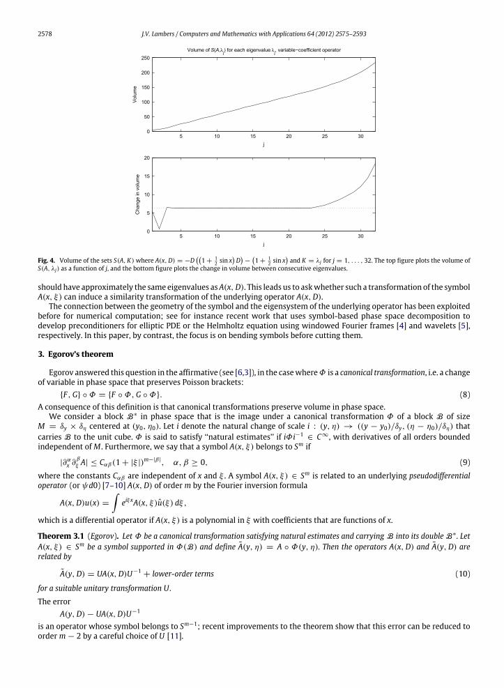
SAK principle suggests that the eigenfunctions of A(x,D) are concentrated in curved boxes of volume ≥ 1, where thegeometry of these boxes is determined by the sets S(A, K). Corresponding to Figs. 2 and 4 shows the volumes of the setsS(A, λj) for the variable-coefficient operator A(x,D) featured in Fig. 3. As in the constant-coefficient case, the set differencesS(A, λj)− S(A, λj−1) have approximate area 2π . This ceases to be true for the largest eigenvalues, but those eigenvalues arenot good approximations to the actual eigenvalues of A(x,D) due to the limited resolution of the discretization.

These figures suggest that it is possible to construct a change of variable Φ : (y, η) → (x, ξ) in phase space in orderto ‘‘bend’’ A(x, ξ) so that it more closely resembles the symbol of a constant-coefficient operator. If Φ preserves volumein phase space, then the volume of each set S(A, K) is invariant under Φ , and therefore an operator with the symbol A ◦ Φ


Fig. 4. Volume of the sets S(A, K)where A(x,D) = −D1 +

12 sin x

D−

1 +

12 sin x

and K = λj for j = 1, . . . , 32. The top figure plots the volume of

S(A, λj) as a function of j, and the bottom figure plots the change in volume between consecutive eigenvalues.

should have approximately the same eigenvalues asA(x,D). This leads us to askwhether such a transformation of the symbolA(x, ξ) can induce a similarity transformation of the underlying operator A(x,D).

The connection between the geometry of the symbol and the eigensystem of the underlying operator has been exploitedbefore for numerical computation; see for instance recent work that uses symbol-based phase space decomposition todevelop preconditioners for elliptic PDE or the Helmholtz equation using windowed Fourier frames [4] and wavelets [5],respectively. In this paper, by contrast, the focus is on bending symbols before cutting them.

3. Egorov’s theorem

Egorov answered this question in the affirmative (see [6,3]), in the casewhereΦ is a canonical transformation, i.e. a changeof variable in phase space that preserves Poisson brackets:

{F ,G} ◦ Φ = {F ◦ Φ,G ◦ Φ}. (8)A consequence of this definition is that canonical transformations preserve volume in phase space.

We consider a block B∗ in phase space that is the image under a canonical transformation Φ of a block B of sizeM = δy × δη centered at (y0, η0). Let i denote the natural change of scale i : (y, η) → ((y − y0)/δy, (η − η0)/δη) thatcarries B to the unit cube. Φ is said to satisfy ‘‘natural estimates’’ if iΦi−1

∈ C∞, with derivatives of all orders boundedindependent ofM . Furthermore, we say that a symbol A(x, ξ) belongs to Sm if

|∂αx ∂β

ξ A| ≤ Cαβ(1 + |ξ |)m−|β|, α, β ≥ 0, (9)

where the constants Cαβ are independent of x and ξ . A symbol A(x, ξ) ∈ Sm is related to an underlying pseudodifferentialoperator (or ψd0) [7–10] A(x,D) of orderm by the Fourier inversion formula

A(x,D)u(x) =

eiξxA(x, ξ)u(ξ) dξ,

which is a differential operator if A(x, ξ) is a polynomial in ξ with coefficients that are functions of x.

Theorem 3.1 (Egorov). Let Φ be a canonical transformation satisfying natural estimates and carrying B into its double B∗. LetA(x, ξ) ∈ Sm be a symbol supported in Φ(B) and define A(y, η) = A ◦ Φ(y, η). Then the operators A(x,D) and A(y,D) arerelated by

A(y,D) = UA(x,D)U−1+ lower-order terms (10)

for a suitable unitary transformation U.

The errorA(y,D)− UA(x,D)U−1

is an operator whose symbol belongs to Sm−1; recent improvements to the theorem show that this error can be reduced toorderm − 2 by a careful choice of U [11].


For ‘‘most’’Φ (see [6,3]), the operator U is given explicitly as a Fourier integral operator [12,13,10]

Uf (y) =

e(y, ξ)eiS(y,ξ) f (ξ) dξ, e ∈ S0, S ∈ S1, (11)

where the function S is related toΦ by

Φ(y, η) = (x, ξ) ⇐⇒ ηk =∂S∂yk

, xk =∂S∂ξk

. (12)

This choice of S is based on theneed to guarantee a valid canonical transformation between the two sets of variables,meaningthat the form of the Hamiltonian is preserved. By Liouville’s Theorem, this condition implies the preservation of volume inphase space [14].

The function S(y, ξ) is called a generating function for the transformation Φ . In the case of a canonical transformationinduced by a change of variable y = φ(x), S(y, ξ) = ξ · φ−1(y) and the factor e(y, ξ) = | detDφ−1(y)|−1/2 is added to makeU unitary, and therefore Uf (y) = | detDφ−1(y)|−1/2(f ◦ φ−1)(y).

It should be noted that while Egorov’s theorem applies to operators supported in a curved box in phase space, it appliesto general differential operators when the canonical transformation Φ arises from a change of variable y = φ(x), providedthatΦ satisfies the natural estimates required by the theorem.

Our goal is to construct unitary similarity transformations that will have the effect of smoothing the coefficients of avariable-coefficient ψd0A(x,D). In the spirit of Egorov’s theorem, we will construct such transformations by acting on thesymbol A(x, ξ).

4. Symbolic calculus and anti-differential operators

We will rely on the rules of symbolic calculus to work with pseudodifferential operators, or ψd0, more easily and thusperform similarity transformations of such operators with much less computational effort than would be required if wewere to apply transformations that acted on matrices representing discretizations of these operators.

4.1. Basic rules of symbolic calculus

We will be constructing and applying unitary similarity transformations of the form

L(x,D) = U∗L(x,D)U (13)

where U is a ψd0. In such cases, it is necessary to be able to compute the adjoint of a ψd0, as well as the product of ψd0.To that end, given an mth-order differential operator A(x,D) whose symbol A(x, ξ) belongs to Sm, the symbol of the

adjoint A∗(x,D) is given by Fefferman [3]

A∗(x, ξ) =

α

(−i)α

α!

∂α

∂xα∂α

∂ξαA(x, ξ). (14)

Similarly, if the nth-order differential operator B(x,D) has symbol B(x, ξ) ∈ Sn, the symbol of the product A(x,D)B(x,D),denoted by AB(x, ξ), is given by

AB(x, ξ) =

α

(−i)α

α!

∂αA∂ξα

∂αB∂αx

. (15)

The terms of these series are symbols of lower order (m − α in (14) and m + n − α in (15)), thus the sums are formallyasymptotic.

These rules are direct consequences of the product rule for differentiation. Without loss of generality, we assume

A(x,D) = a(x)Dj, B(x,D) = b(x)Dk

where the coefficients a(x) and b(x) are real. Then

A∗(x, ξ) = e−iξxA∗(x,D)eiξx

= e−iξx(−1)jDj[a(x)eiξx]

= e−iξxi−j dj

dxj[a(x)eiξx]

= i−jj

ℓ=0

jℓ

dℓa(x)dxℓ

(iξ)j−ℓ


=

jℓ=0

1ℓ!

dℓ

dxℓ

j!

(j − ℓ)!i−ℓa(x)(ξ)j−ℓ

=

jℓ=0

(−i)ℓ

ℓ!

dℓ

dξ ℓdℓ

dxℓa(x)(ξ)j

=

ℓ

(−i)ℓ

ℓ!

∂ℓ

∂ξ ℓ

∂ℓ

∂xℓA(x, ξ).

Similarly,

AB(x, ξ) = e−iξxA(x,D)B(x,D)eiξx

= ξ ke−iξxa(x)Dj[b(x)eiξx]

= ξ ka(x)i−jj

ℓ=0

j!ℓ!(j − ℓ)!

dℓb(x)dxℓ

(iξ)j−ℓ

=

jℓ=0

(−i)ℓ

ℓ!a(x)

j!(j − ℓ)!

ξ j−ℓ∂ℓB(x, ξ)∂xℓ

=

jℓ=0

(−i)ℓ

ℓ!

∂ℓA(x, ξ)∂ξ ℓ

∂ℓB(x, ξ)∂xℓ

.

4.2. The pseudo-inverse of the differentiation operator

For general ψd0, the rules (14), (15) do not always apply, but they do yield an approximation. However, it will benecessary for us to workwithψd0 of negative order, so wemust identify a class of negative-orderψd0 for which these rulesdo apply, as closely as possible. It makes sense to consider describing operators of negative order using anti-differentiation,as differentiation operators are of positive order, but as they are also singular, it is necessary to specify a particularantiderivative.

Let A be an m × n matrix of rank r , and let A = UΣV T be the singular value decomposition of A, where UTU = Im,V TV = In, andΣ = diag(σ1, . . . , σr , 0, . . . , 0). Then, the pseudo-inverse (see [15]) of A is defined as

A+= VΣ+UT , (16)

where the n × m diagonal matrixΣ+ is given by

Σ+=

σ−11

. . .

σ−1r

0. . .

0

. (17)

We can generalize this concept to define the pseudo-inverse of the differentiation operator D on the space of 2π-periodicfunctions by

D+u(x) =i

√2π

∞ω=−∞

eiωxω+u(ω), (18)

where

ω+=

ω−1 ω = 00 ω = 0. (19)

The effect of this operator on a function u(x) is to compute the antiderivative of each Fourier component of u(x), with aconstant of integration of zero, except for the component corresponding to ω = 0. Equivalently,

D+u(x) = i

+0[u(s)− Avg u] dx,


where the subscript of+0 of the integral sign indicates that indefinite integration is performed, but a constant of integrationof zero is assumed to ensure uniqueness. It is also interesting to note that

DD+u(x) = D+Du(x) =i

√2π

∞ω=−∞,ω=0

eiωxu(ω) = u(x)− Avg u.

The rules (14) and (15) can be used for pseudodifferential operators defined using D+, at least up to a symbol of lowerorder.

Lemma 4.1. Let A(x,D) be the anti-differential operator defined by

A(x,D)u = D+[a(x)u], (20)

where a(x) ∈ Cnp [0, 2π ]. Then

A(x, ξ) =

n−1α=0

iαdαaξ (x)dxα

(ξ+)α+1+ (iξ+)ne−iξxD+

[a(n)ξ (x)eiξx

], (21)

where

aξ (x) = a(x)−1

√2π

a(−ξ)e−iξx. (22)

Proof. Using the definition of A(x, ξ) and integration by parts, we obtain, for ξ = 0,

A(x, ξ) = e−iξxA(x,D)eiξx

= e−iξxD+[a(x)eiξx]

= e−iξxi

+0

a(x)eiξx − Avg a(x)eiξx

dx

= e−iξxi

+0

a(x)eiξx −

12π

2π

0a(y)eiξy dy

dx

= e−iξxi

+0

a(x)eiξx −

1√2π

a(−ξ)

dx

= e−iξxi

+0

a(x)−

1√2π

a(−ξ)e−iξxeiξx dx

= e−iξxi

+0aξ (x)eiξx dx

= e−iξxi1iξ

aξ (x)eiξx −1iξ

+0

a′

ξ (x)eiξx dx

= aξ (x)ξ+

+ iξ+e−iξxD+[a′

ξ (x)eiξx

].

Applying repeatedly yields (21). �

It follows that (15) applies to the product of D+ and a(x), but only approximately. However, the error

E(x, ξ) = e−iξxi

+0

1√2π

a(−ξ)e−iξxeiξx dx

=i

√2π

a(−ξ)xe−iξx dx,

which is a symbol of order −(n + 1), due to the smoothness of a(x) that determines the rate of decay of its Fouriercoefficients [16]. We now consider adjoints and products involving both anti-differential and differential operators.

Proposition 4.2. The rules (14) and (15) approximately hold for anti-differential operators of the form

A(x,D) = a(x)(D+)k, k > 0 (23)


that belong to S−k, and differential operators L(x,D) of the form (1). That is, if the coefficient a(x) belongs to C∞p [0, 2π ], as do

the coefficients of L(x,D), then for ξ = 0,

A∗(x, ξ) =

α

(−i)α

α!

∂α

∂xα∂α

∂ξαA(x, ξ)+ E1(x, ξ), (24)

AL(x, ξ) =

α

(−i)α

α!

∂αA∂ξα

∂αB∂αx

+ E2(x, ξ), (25)

and

LA(x, ξ) =

α

(−i)α

α!

∂αA∂ξα

∂αB∂αx

, (26)

where E1(x, ξ), E2(x, ξ) are symbols of arbitrarily large negative order.

Proof. Without loss of generality, wewill assume L(x,D) = b(x)Dj where j ≥ 0. Then, by repeated application of Lemma4.1,we have

A∗(x, ξ) = e−iξx(D+)k[a(x)eiξx]

≈

∞α=0

iαα + k − 1

α

dαaξ (x)dxα

(ξ+)α+k

≈

∞α=0

iα

α!(−1)α

(α + k − 1)!(k − 1)!

dαaξ (x)dxα

(ξ+)α+k

≈

∞α=0

(−i)α

α!

dα

dξα(ξ+)k

dαaξ (x)dxα

≈

∞α=0

(−i)α

α!

∂α

∂xα∂α

∂ξαA(x, ξ)

which is (14). The error in the approximation arises from the first application ofD+ to a(x)eiξx, as described in Lemma4.1. Theresulting error in A∗(x, ξ) is of the form E1(x, ξ) = pk(x)a(−ξ)e−iξx,where pk(x) is a polynomial of degree k, and thereforeE1(x, ξ) is a symbol of arbitrarily large negative order, due to the decay rate of the Fourier coefficients of a(x) ∈ C∞

p [0, 2π ].Next, we have

AL(x, ξ) = e−iξxa(x)(D+)k[b(x)Djeiξx]≈ e−iξxξ ja(x)(D+)k[b(x)eiξx]

≈ ξ ja(x)∞α=0

iαα + k − 1

α

dαb(x)dxα

(ξ+)α+k

=

∞α=0

iα

α!a(x)(−1)k

(α + k − 1)!(k − 1)!

∂αL∂xα

=

∞α=0

(−i)α

α!

∂αA∂ξα

∂αL∂xα

which is (15). The error in the approximation arises from the first application of D+ to b(x)eiξx, as described in Lemma 4.1.The resulting error in AL(x, ξ) is of the form E2(x, ξ) = a(x)qk(x)b(−ξ)e−iξx(ξ)j, where qk(x) is a polynomial of degreek, and therefore E2(x, ξ) is a symbol of arbitrarily large negative order, due to the decay rate of the Fourier coefficients ofb(x) ∈ C∞

p [0, 2π ].Finally, we consider

LA(x, ξ) = e−ixixb(x)Dja(x)(D+)keiξx

= (−i)jb(x)j

α=0

jα

dja(x)dxj

(iξ)j−α ik(ξ+)k

=

jα=0

(−i)α

α!

∂αL∂ξα

∂αA∂xα

,

which is (15). �


This result allows us to use symbolic calculus to develop heuristics that aid in the construction of unitary similaritytransformations based on ψd0 of the form

U(x,D) =

∞α=0

aα(x)(D+)−α. (27)

Such transformations will be considered in Section 6.

5. Local preconditioning

A special case that is useful for practical computation is whereΦ arises from a simple change of variable y = φ(x), whereφ(x) is a differentiable function and

φ′(x) > 0,12π

2π

0φ′(s) ds = 1. (28)

The transformationΦ has the form

Φ(y, η) → (x, ξ), x = φ−1(y), ξ = φ′(x)η. (29)In this case, we set e(y, ξ) = | detDφ−1(y)|1/2 and S(y, ξ) = φ−1(y)ξ , and the Fourier inversion formula yields Uf (y) =

| detDφ−1(y)|1/2f ◦ φ−1(y).Suppose that L(x,D) is an mth order differential operator such that the leading coefficient am(x) does not change sign.

Using this simple canonical transformation, we can precondition a differential operator L(x,D) as follows: Choose φ(x) andconstruct a canonical transformationΦ(y, η) by (29) so that the transformed symbol

L(y, η) = L(x, ξ) ◦ Φ(y, η) = L(φ−1(y), φ′(φ−1(y))η) (30)resembles a constant-coefficient symbol as closely as possible for a fixed frequency η0 in transformed phase space. This willyield a symbol L(y, η) that is smooth in a region of phase space concentrated around η = η0. Then, we can select anothervalue for η0 and repeat, until our symbol is sufficiently smooth in the region of phase space {(y, η)||η| < N/2}.

Sincewe are using a canonical transformation based on a change of spatial variable y = φ(x), we can conclude by Egorov’stheorem that there exists a unitary Fourier integral operator U such that if A = U−1LU , then the symbol of A agrees with Lmodulo lower-order errors. Using the chain rule and symbolic calculus, it is a simple matter to construct this new operatorA(y,D).

We will now illustrate the process for a second-order self-adjoint operator

L(x,D) = a2(x)D2+ a′

2(x)D + a0(x), (31)with symbol

L(x, ξ) = a2(x)ξ 2 − a′

2(x)iξ + a0(x). (32)We will attempt to smooth out this symbol in a region of phase space concentrated around the line η = η0. Our goal is tochoose φ(x) so that the canonical transformation (29) yields a symbol L(y, η) satisfying L(y, η0) is independent of y. In thiscase, the expression L(φ−1(y), φ′(φ−1(y))η0) would also be independent of y, and therefore we can reduce the problem tothat of choosing φ so that L(x, φ′(x)η0) is independent of x.

The result is, for each x, a polynomial equation in φ′(x),

a2(x)φ′(x)2η20 − ia′

2(x)φ′(x)η0 + a0(x) = Lη0 , (33)

where the constant Lη0 is independent of x. This equation cannot be solved exactly for a real-valued φ′(x), but we can tryto solve it approximately in some sense. For example, we can choose a real constant Lη0 , perhaps as the average value ofL(x, η0) over the interval [0, 2π ], and then choose φ(x) in order to satisfy

a2(x)φ′(x)2η20 + a0(x) = Lη0 (34)at each gridpoint, which yields

φ′(x) = cη0

Avg a2a2(x)

+Avg a0 − a0(x)

a2(x)η20, (35)

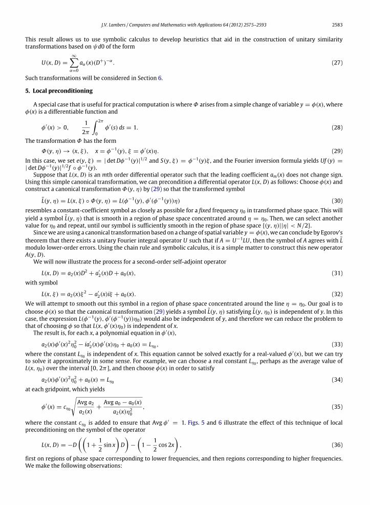
where the constant cη0 is added to ensure that Avg φ′= 1. Figs. 5 and 6 illustrate the effect of this technique of local

preconditioning on the symbol of the operator

L(x,D) = −D

1 +12sin x

D

−

1 −

12cos 2x

, (36)

first on regions of phase space corresponding to lower frequencies, and then regions corresponding to higher frequencies.We make the following observations:


Fig. 5. Local preconditioning applied to operator L(x,D)with η0 = 4 to obtain new operator L(y,D).

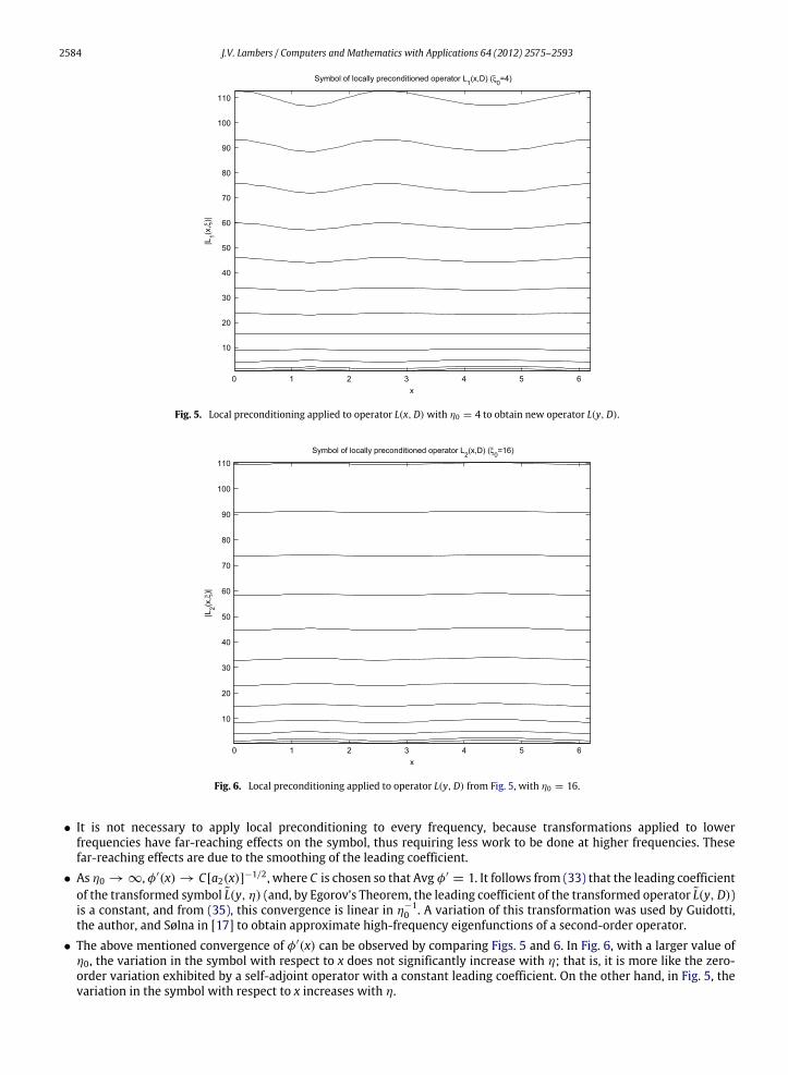
Fig. 6. Local preconditioning applied to operator L(y,D) from Fig. 5, with η0 = 16.

• It is not necessary to apply local preconditioning to every frequency, because transformations applied to lowerfrequencies have far-reaching effects on the symbol, thus requiring less work to be done at higher frequencies. Thesefar-reaching effects are due to the smoothing of the leading coefficient.

• As η0 → ∞, φ′(x) → C[a2(x)]−1/2, where C is chosen so that Avg φ′= 1. It follows from (33) that the leading coefficient

of the transformed symbol L(y, η) (and, by Egorov’s Theorem, the leading coefficient of the transformed operator L(y,D))is a constant, and from (35), this convergence is linear in η−1

0 . A variation of this transformation was used by Guidotti,the author, and Sølna in [17] to obtain approximate high-frequency eigenfunctions of a second-order operator.

• The above mentioned convergence of φ′(x) can be observed by comparing Figs. 5 and 6. In Fig. 6, with a larger value ofη0, the variation in the symbol with respect to x does not significantly increase with η; that is, it is more like the zero-order variation exhibited by a self-adjoint operator with a constant leading coefficient. On the other hand, in Fig. 5, thevariation in the symbol with respect to x increases with η.


6. Global preconditioning

It is natural to ask whether it is possible to construct a unitary transformation U that smoothes L(x,D) globally, i.e. yieldthe decomposition

U∗L(x,D)U = L(η). (37)

In this section, we will attempt to answer this question. We begin by examining a simple eigenvalue problem, and thenattempt to generalize the solution technique employed.

Consider a first-order differential operator of the form

L(x,D) = a1D + a0(x), (38)

where a0(x) is a 2π-periodic function. We will solve the eigenvalue problem

L(x,D)u(x) = λu(x), 0 < x < 2π, (39)

with periodic boundary conditions

u(x) = u(x + 2π), −∞ < x < ∞. (40)

This eigenvalue problem is a first-order linear differential equation

a1u′(x)+ a0(x)u(x) = λu(x). (41)

Because the coefficients are periodic, we can apply Floquet’s Theorem [18] to conclude that the fundamental solution uλ(x)satisfies

uλ(x + 2π) = uλ(x)[uλ(0)]−1uλ(2π),

where

uλ(x) = exp x

0

λ− a0(s)a1

ds.

The periodic boundary conditions can be used to determine the eigenvalues of L(x,D). Specifically, uλ(x) must satisfyuλ(0) = uλ(2π), which yields the condition 2π

0

λ− a0(s)a1

ds = i2πk, (42)

for some integer k. If we denote by Avg a0 the average value of a0(x) on the interval [0, 2π ],

Avg a0 =12π

2π

0a0(s) ds, (43)

then the periodicity of uλ(x) yields the discrete spectrum of L(x,D),

λk = Avg a0 + ia1k, (44)

for all integers k, with corresponding eigenfunctions

uk(x) = exp x

0

Avg a0 − a0(s)a1

ds + ikx. (45)

Let

v(x) = exp x

0

Avg a0 − a0(s)a1

ds. (46)

Then uk(x) = v(x)eikx and

[v(x)]−1L(x,D)v(x)eikx = λkeikx. (47)

We have succeeded in diagonalizing L(x,D) by using the zeroth-order symbol v(x) to perform a similarity transformationof L(x,D) into a constant-coefficient operator

L(x,D) = [v(x)]−1L(x,D)v(x) = a1D + Avg a0. (48)

The same technique can be used to transform anmth-order differential operator of the form

L(x,D) = amDm+

m−1α=0

aα(x)Dα, (49)


so that the constant coefficient am is unchanged and the coefficient am−1(x) is transformed into a constant equal toam−1 = Avg am−1. This is accomplished by computing L(x,D) = [vm(x)]−1L(x,D)vm(x)where

vm(x) = exp x

0

Avg am−1 − am−1(s)mam

ds. (50)

Note that ifm = 1, then we have v1(x) = v(x), where v(x) is defined in (46).We now seek to generalize this technique in order to eliminate lower-order variable coefficients. The basic idea is to

construct a transformation Uα such that

1. Uα is unitary;2. The transformation L(x,D) = U∗

αL(x,D)Uα yields an operator L(x,D) =m

β=−∞bβ(x)

∂∂x

βsuch that aα(x) is constant;

and3. The coefficients aβ(x) of L(x,D), where β > α, are invariant under the similarity transformation L = U∗

αL(x,D)Uα .

It turns out that such an operator is not difficult to construct. First, we note that if φ(x,D) is a skew-symmetricpseudodifferential operator, then U(x,D) = exp[φ(x,D)] is a unitary operator, since

U(x,D)∗U(x,D) = (exp[φ(x,D)])∗ exp[φ(x,D)]= exp[−φ(x,D)] exp[φ(x,D)]= I.

We consider an example to illustrate how one can determine a operator φ(x,D) so that U(x,D) = exp[φ(x,D)] satisfiesthe second and third conditions given above. Given a second-order self-adjoint operator of the form (31), we know thatwe can use a canonical transformation to make the leading-order coefficient constant, and since the corresponding Fourierintegral operator is unitary, symmetry is preserved, and therefore our transformed operator has the form

L(x,D) = a2D2+ a0(x). (51)

In an effort to transform L so that the zeroth-order coefficient is constant, we apply the similarity transformation L = U∗LU ,which yields an operator of the form

L = e−φLeφ

= e−ad(φ)L

= L + [L, φ] +12[[L, φ], φ] + · · · (52)

where ad(X)Y = [X, Y ] [19].Since we want the first and second-order coefficients of L to remain unchanged, the perturbation E of L in L = L + E

must not have order greater than zero. If we require that φ has negative order −k, then the highest-order term in E is[L, φ] = Lφ − φL, which has order 1− k, so in order to affect the zero-order coefficient of Lwemust have φ be of order −1.

By symbolic calculus, it is easy to determine that the highest-order coefficient of Lφ − φL is 2a2b′

−1(x) where b−1(x) isthe leading coefficient of φ. Therefore, in order to satisfy

a0(x)+ 2a2b′

−1(x) = constant, (53)

we must have b′

−1(x) = −(a0(x)− Avg a0)/2a2. In other words,

b−1(x) = −12a2

D+(a0(x)), (54)

whereD+ is the pseudo-inverse of the differentiation operatorD introduced in Section 4. Therefore, for our operatorφ(x,D),we can use

φ(x,D) =12[b−1(x)D+

− (b−1(x)D+)∗]

= b−1(x)D++ lower-order terms. (55)

Using symbolic calculus, it can be shown that the coefficient of order −1 in L is zero. To see this, we first note that withφ being of order −1, in the previously described expansion

L = L + [L, φ] +12[[L, φ], φ] + · · · ,

the third term is of order −2, due to the terms corresponding to α = 0 in (15) being canceled in the commutator, so thisterm (and subsequent terms, which are of still lower order) need not be examined.


Next, we note that

[L, φ]∗

= (Lφ − φL)∗ = φ∗L∗− L∗φ∗

= −φL + Lφ = [L, φ].

Furthermore, we have

L + [L, φ] = a2D2+ (Avg a0)− ia−1(x)D+

+ lower-order terms.

However, the leading-order portion a2D2+ (Avg a0) is self-adjoint, which implies that the remainder −ia−1(x)D+

+

lower-order terms is also self-adjoint. By (14), the leading-order term of the adjoint is ia−1(x)D+, and therefore we musthave a−1(x) ≡ 0.

More generally, suppose that L(x,D) is an mth-order operator of the form (49) whose leading-order variable coefficientam−1(x) has also been homogenized by a transformation of the form L(x,D) = [vm(x)]−1L(x,D)vm(x)where vm(x) is definedby (50), to yield an operator of the form

L(x,D) = amDm+ am−1Dm−1

+

m−2α=0

aα(x)Dα.

In order to transform L(x,D) so that am−2(x) is also made constant, we use a similarity transformation of the form L(x, E) =

U(x,D)∗LU(x,D), where U(x,D) = exp[φ(x,D)] and φ(x,D) is an anti-self-adjoint operator; that is, φ∗(x,D) = −φ(x,D).As in the preceding example involving a second-order operator, we examine the leading-order term of the deviation of

L = U∗LU from L, which is given by Lφ − φL. By requiring that φ is of order −1, we ensure that this term is of order m − 2,in view of (15), if we stipulate that

φ(x,D) =12[ϕ(x,D)− ϕ∗(x,D)], ϕ(x,D) = b−1(x)D+,

which, by (14), yields

φ(x,D) = b−1(x)D++ lower-order terms.

We then have

Lφ − φL = mamb′

−1(x)Dm−2

+ lower-order terms.

Therefore, in order to ensure that the term of orderm − 2 in the transformed operator has a constant coefficient, we set

b−1(x) = −1

mamD + (am−2(x)),

by analogy with (54). If L is also self-adjoint (for m even) or skew-self-adjoint (for m odd), then am−1 = 0 and afterhomogenizing am−2(x), the coefficient of order m − 3 in the transformed operator L is zero, just as the coefficient of order−1 in the transformed second-order operator L is zero.

We can use similar transformations to make lower-order coefficients constant as well. In doing so, the following resultis helpful:

Proposition 6.1. Let L(x,D) be an mth order self-adjoint pseudodifferential operator of the form

L(x,D) =

m−∞

aα(x)iαDα, (56)

where we define D−k= (D+)k for k > 0 and the coefficients {aα(x)} are all real. For any odd integer α0, if aα(x) is constant for

all α > α0, then aα0(x) ≡ 0.

Proof. Because the leading-order portion of L(x,D),

Lm(x,D) =

mα=α0+1

aα iαDα

is constant-coefficient, and must itself be self-adjoint, the reminder

L0(x,D) =

α0α=−∞

aα(x)iαDα

must also be self-adjoint. We then have, by (14),

L∗

0(x, ξ) = L0(x, ξ)+ lower-order terms = −iα0aα0(x)ξα0 + lower-order terms. (57)

Because α0 is odd, this implies that aα0(x) = −aα0(x), from which the result follows. �


Example. Let L(x,D) = D2+ sin x. Let

b−1(x) =12cos x (58)

and

φ(x,D) =14[cos xD+

− (cos xD+)∗]

=12(cos x)D+

+ lower-order terms. (59)

Then, since Avg sin x = 0, it follows that

L(x,D) = U∗

αL(x,D)Uα= exp[−φ(x,D)]L(x,D) exp[φ(x,D)]= D2

+ E(x,D),

where E(x,D) is of order −2. �

6.1. Non-normal operators

If the operator L(x,D) is not normal, then it is not unitarily diagonalizable, and therefore cannot be approximatelydiagonalized using unitary transformations. Instead, we can use similarity transformations of the form

L(x,D) = exp[−φ(x,D)]L(x,D) exp[φ(x,D)], (60)where φ(x) is obtained in the same way as for self-adjoint operators, except that we do not take its skew-symmetric part.For example, if L(x,D) = a2D2

+ a1D + a0(x), then we can make the zeroth-order coefficient of L(x,D) constant by setting

φ(x) = b−1(x)D+= −

12a2

D+(a0(x))D+. (61)

In this case, the variable-coefficient remainder is of order −1, rather than −2 as in the self-adjoint case.

6.2. Operators in higher spatial dimensions

Consider the operator L(x,D) = a2∆ + a0(x), defined on the n-dimensional cube [0, 2π ]n. Using symbolic calculus,

by analogy with (54), it can be shown that the zero-order coefficient a0(x) can be homogenized through the similaritytransformation U∗LU , where

U(x,D) = exp[(φ(x,D)− φ∗(x,D))/2], (62)

φ(x, ξ) = −1

(2π)n/2

ω∈Zn,ω=0

φω(x, ξ , ω), ξ = 0, (63)

where

φω(x, ξ , ω) =

a0(ω)eiω·x

2ia2(ω · ξ)ω · ξ = 0

a0(ω)(ξ · x)eiω·x

2ia2(ξ · ξ)ω · ξ = 0

. (64)

This can be seen by equating the zeroth-order term of (52) to a constant a0, using a higher-dimensional analogue of (15),and then solving for φ(x, ξ). That is,

a0 = a0(x)+ in

j=1

∂L(x, ξ)∂ξj

∂φ(x, ξ)∂xj

= a0(x)+ 2ia2n

j=1

ξj∂φ(x, ξ)∂xj

which yields

∇xφ(x, ξ ) · ξ =Avg a0 − a0(x)

2ia2.

Expressing a0(x) in terms of its discrete Fourier series and solving this equation leads to (64). Future work will explore theefficient implementation of such transformations using discrete symbol calculus [20].


7. Implementation

The rules for symbolic calculus introduced in Section 4 can easily be implemented andprovide a foundation for algorithmsto perform unitary similarity transformations on pseudodifferential operators. In this section we will develop practicalimplementations of the local and global preconditioning techniques discussed in Sections 5 and 6.

7.1. Simple canonical transformations

First, we will show how to efficiently transform a differential operator L(x,D) into a new differential operator L(y,D) =

U∗L(x,D)U where U is a Fourier integral operator related to a canonical transformation Φ(y, η) = (x, ξ) by Egorov’sTheorem. For clarity wewill assume that L(x,D) is a second-order operator, but the resulting algorithm can easily be appliedto operators of arbitrary order.

Algorithm 7.1. Given a self-adjoint differential operator L(x,D) and a functionφ′(x) satisfyingφ′(x) > 0 and 2π0 φ′(x) dx =

1, the following algorithm computes the differential operator L = U∗LU where Uf (x) =√φ′(x)f (φ(x)).

φ = x0 φ

′(s) dsL = φ−1/2Lφ1/2

C1 = 1L = 0for j = 0, . . . ,m,

for k = j + 1, . . . , 2,Ck = C ′

k + Ck−1φ′

endLj = 0for k = 0, . . . , j,

Lj = Lj + ((ajCk+1) ◦ φ−1)Dk

endL = L + Lj

end

This algorithm requires O(N logN) floating-point operations, assuming that each function is discretized on an N-point gridand that the fast Fourier transform is used for differentiation.

7.2. Eliminating variable coefficients

Supposewewish to transformanmth-order self-adjoint differential operator L(x,D) into L(x,D) = Q ∗(x,D)L(x,D)Q (x,D)where coefficients of order J and above are constant. After we apply Algorithm 7.1 to make am(x) constant, we can proceedas follows:j = m − 2k = 1while j >= J

Let aj(x) be the coefficient of order j in L(x,D)φj = D+(aj(x)/2am(x))Let E(x,D) = φj(x)(D+)k

Let Q (x,D) = exp[(E(x,D)− E∗(x,D))/2]L(x,D) = Q ∗(x,D)L(x,D)Q (x,D)j = j − 2k = k + 2

endSince L(x,D) is self-adjoint, this algorithm is able to take advantage of Proposition 6.1 to avoid examining odd-ordercoefficients.

In a practical implementation, one should be careful in computing Q ∗LQ . Using symbolic calculus, there is muchcancellation among the coefficients. However, it is helpful to note that from (52),

exp[−A(x,D)]L(x,D) exp[A(x,D)] =

∞ℓ=0

1ℓ!

Cℓ(x,D), (65)

where the operators {Cℓ(x,D)} satisfy the recurrence relation

C0 = L,Cℓ = Cℓ−1A − ACℓ−1, ℓ > 0,


Fig. 7. Symbol of original variable-coefficient operator P(x,D) defined in (66).

and each Cℓ(x,D) is of order m + ℓ(k − 1), where k < 0 is the order of A(x,D). Expressions of the form A(x,D)B(x,D) −

B(x,D)A(x,D) can be computed without evaluating the first term in (15) for each of the two products, since it is clear that itwill be cancelled.

The operator Q (x,D) must be represented using a truncated series. In order to ensure that all coefficients of L(x,D)of order J or higher are correct, it is necessary to compute terms of order J − m or higher. With this truncated seriesrepresentation of Q (x,D) in each iteration, the algorithm requires O(N logN) floating-point operations when an N-pointdiscretization of the coefficients is used and the fast Fourier transform is used for differentiation. It should be noted, however,that the number of terms in the transformed operator L(x,D) can be quite large, depending on the choice of J .

7.3. Using multiple transformations

When applying multiple similarity transformations such as those implemented in this section, it is recommended that avariable-grid implementation be used in order to represent transformed coefficients as accurately as possible. In applyingthese transformations, errors are introduced by pointwise multiplication of coefficients and computing composition offunctions using interpolation, and these errors can accumulate very rapidly when applying several transformations.

8. Numerical results

In this section we will illustrate the effects of preconditioning on differential operators. We will use the operator thatwas first introduced in (36) to illustrate local preconditioning,

P(x,D) = −D

1 +12sin x

D

−

1 −

12cos 2x

. (66)

8.1. Preconditioning

Fig. 7 shows the symbol P(x, ξ) before preconditioning is applied. Fig. 8 shows the symbol of A = U∗PU where U is aFourier integral operator induced by a canonical transformation that makes the leading coefficient constant. Finally, Fig. 9shows the symbol of B = Q ∗AQ where Q is designed to make the zero-order coefficient of A constant, using the techniquedescribed in Section 6. The transformation U smooths the symbol of P(x,D) so that the curvature in the surface definedby |A(x, ξ)| has uniform curvature with respect to ξ . The transformation Q yields a symbol that closely resembles that of aconstant-coefficient operator except at the lowest frequencies.

8.2. Approximating eigenfunctions

By applying the preconditioning transformations to Fourier waves eiωx, excellent approximations to eigenvalues andeigenfunctions can be obtained. This follows from the fact that if the operator Q ∗L(x,D)Q is close to a constant-


Fig. 8. Symbol of transformed operator A(x,D) = U∗P(x,D)U where P(x,D) is defined in (66) and U is chosen to make the leading coefficient of A(x,D)constant.

Fig. 9. Symbol of transformed operator B(x,D) = Q ∗U∗L(x,D)UQ where P(x,D) is defined in (66) and the unitary similarity transformations Q and Umake B(x,D) a constant-coefficient operator modulo terms of negative order.

coefficient operator, then eiωx is an approximate eigenfunction of Q ∗L(x,D)Q , and therefore Qeiωx should be an approximateeigenfunction of L(x,D).

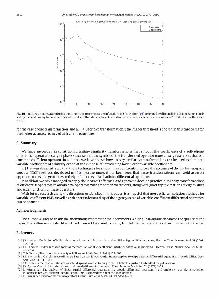
Let L(x,D) = P(x,D) from (66). Fig. 10 displays the relative error, measured using the L2 norm, in eigenfunctionscorresponding to the lowest 40 eigenvalues of P(x,D). In the first experiment, the transformation Q makes the second-order and zeroth-order coefficients constant, using the techniques presented in Sections 5 and 6. In the second experiment,an additional transformation is used to make the coefficient of order −2 constant. We observe that the accuracy of theapproximate eigenfunctions increases rapidly with the frequency, and this improvement is much more dramatic when asecond transformation is used.

It should be noted that this strategy does not work well for low frequencies. However, it does largely orthogonalizeeigenfunctions corresponding to low frequencies against high-frequency waves, which allows computation of accurateeigenfunctions by restricting to a much coarser grid. In the results shown in Fig. 10, this approach is used for |ω| ≤ 4


Fig. 10. Relative error, measured using the L2 norm, in approximate eigenfunctions of P(x,D) from (66) generated by diagonalizing discretization matrixand by preconditioning to make second-order and zeroth-order coefficients constant (solid curve) and coefficient of order −2 constant as well (dashedcurve).

for the case of one transformation, and |ω| ≤ 8 for two transformations; the higher threshold is chosen in this case tomatchthe higher accuracy achieved at higher frequencies.

9. Summary

We have succeeded in constructing unitary similarity transformations that smooth the coefficients of a self-adjointdifferential operator locally in phase space so that the symbol of the transformed operator more closely resembles that of aconstant-coefficient operator. In addition, we have shown how unitary similarity transformations can be used to eliminatevariable coefficients of arbitrary order, at the expense of introducing lower-order variable coefficients.

In [1] it was demonstrated that these techniques for smoothing coefficients improve the accuracy of the Krylov subspacespectral (KSS) methods developed in [1,2]. Furthermore, it has been seen that these transformations can yield accurateapproximations of eigenvalues and eigenfunctions of self-adjoint differential operators.

In addition, we havemanaged to apply the ideas of Fefferman and Egorov to develop practical similarity transformationsof differential operators to obtain new operatorswith smoother coefficients, alongwith good approximations of eigenvaluesand eigenfunctions of these operators.

With future research along the directions established in this paper, it is hopeful that more efficient solution methods forvariable-coefficient PDE, aswell as a deeper understanding of the eigensystems of variable-coefficient differential operators,can be realized.

Acknowledgments

The author wishes to thank the anonymous referees for their comments which substantially enhanced the quality of thepaper. The authorwould also like to thank Laurent Demanet formany fruitful discussions on the subjectmatter of this paper.

References

[1] J.V. Lambers, Derivation of high-order spectral methods for time-dependent PDE using modified moments, Electron. Trans. Numer. Anal. 28 (2008)114–135.

[2] J.V. Lambers, Krylov subspace spectral methods for variable-coefficient initial-boundary value problems, Electron. Trans. Numer. Anal. 20 (2005)212–234.

[3] C. Fefferman, The uncertainty principle, Bull. Amer. Math. Soc. 9 (1983) 129–206.[4] S.B. Bhowmik, C.C. Stolk, Preconditioners based on windowed Fourier frames applied to elliptic partial differential equations, J. Pseudo-Differ. Oper.

Appl. 2 (2011) 317–342.[5] C.C. Stolk, On the generalization of wavelet diagonal preconditioning to the Helmholtz equation, (submitted for publication).[6] J.V. Egorov, Canonical transformations and pseudodifferential operators, Trans. Moscow Math. Soc. 24 (1975) 1–28.[7] L. Hörmander, The analysis of linear partial differential operators. III, pseudo-differential operators, in: Grundlehren der Mathematischen

Wissenschaften 274, Springer-Verlag, Berlin, 1994. Corrected reprint of the 1985 original.[8] L. Hörmander, Pseudo-differential operators, Comm. Pure Appl. Math. 18 (1965) 501–517.


[9] J.J. Kohn, L. Nirenberg, An algebra of pseudo-differential operators, Comm. Pure Appl. Math. 18 (1965) 269–305.[10] F. Trèves, Introduction to Pseudodifferential and Fourier Integral Operators, in: The University Series in Mathematics, vol. 2, Plenum Press, New

York–London, 1980.[11] J.D. Silva, An accuracy improvement in Egorov’s theorem, Publ. Mat. 51 (2007) 77–120.[12] J.J. Duistermaat, Fourier Integral Operators, in: Progress in Mathematics, vol. 130, Birkhäuser Boston, Inc., Boston, MA, 1996.[13] L. Hörmander, The analysis of linear partial differential operators. IV, Fourier integral operators, in: Grundlehren derMathematischenWissenschaften

275, Springer-Verlag, Berlin, 1994. Corrected reprint of the 1985 original.[14] I. Chavel, Riemannian Geometry: A Modern Introduction, Cambridge University Press, New York, 1994.[15] G.H. Golub, C.F. van Loan, Matrix Computations, third ed., Johns Hopkins University Press, 1996.[16] B. Gustafsson, H.-O. Kreiss, J. Oliger, Time-Dependent Problems and Difference Methods, Wiley, New York, 1995.[17] P. Guidotti, J.V. Lambers, K. Sølna, 1D analysis ofwave propagation in inhomogeneous and randommedia, Numer. Funct. Anal. Optim. 27 (2006) 25–55.[18] G. Floquet, Sur les équations différentielles linéaires à coefficients périodiques, Annales Scientifiques de l’École Normale Supérieure 12 (1883) 47–88.[19] W. Miller, Symmetry Groups and their Applications, Academic Press, New York, 1972, pp. 159–161.[20] L. Demanet, L. Ying, Discrete symbol calculus, SIAM Rev. 53 (2011) 71–104.

Documents

Approximate diagonalization of variable-coefficient differential operators through similarity transformations